accuracy of service area estimation …public.lanl.gov/rbent/cipbook14.pdfchapter 12 accuracy of...

Chapter 12

ACCURACY OF SERVICE AREAESTIMATION METHODS USED FORCRITICAL INFRASTRUCTURERECOVERY

Okan Pala, David Wilson, Russell Bent, Steve Linger and James Arnold

Abstract Electric power, water, natural gas and other utilities are served to con-sumers via functional sources such as electric power substations, pumpsand pipes. Understanding the impact of service outages is vital to deci-sion making in response and recovery efforts. Often, data pertaining tothe source-sink relationships between the service points and consumersis sensitive or proprietary, and is, therefore, unavailable to external en-tities. As a result, during emergencies, decision makers often rely onestimates of service areas produced by various methods. This paper,which focuses on electric power, assesses the accuracy of four meth-ods for estimating power substation service areas, namely the standardand weighted versions of Thiessen polygon and cellular automata ap-proaches. Substation locations and their power outputs are used asinputs to the service area calculation methods. Reference data is usedto evaluate the accuracy in approximating a power distribution networkin a mid-sized U.S. city. Service area estimation methods are surveyedand their performance is evaluated empirically. The results indicatethat the performance of the approaches depends on the type of analysisemployed. When the desired analysis includes aggregate economic orpopulation predictions, the weighted version of the cellular automataapproach has the best performance. However, when the desired analy-sis involves facility-specific predictions, the weighted Thiessen polygonapproach tends to perform the best.

Keywords: Service area estimates, recovery, Thiessen polygon, cellular automata

180 CRITICAL INFRASTRUCTURE PROTECTION VIII

1. IntroductionElectric power, water, natural gas, telecommunications and other utilities are

served to consumers using functional sources (facilities) such as power substa-tions, pumps and pipes, switch controls and cell towers. Each of these sources isrelated to a geographical service area that includes consumers. Data pertainingto the source-sink relationships between service points and consumers is oftensensitive or proprietary and is, therefore, unavailable to external entities. Dur-ing emergencies, decision makers who do not have access to utility informationmust rely on estimates of service areas derived by various methods. Decisionmakers have a strong interest in quantifying the accuracy of critical infras-tructure service area estimation methods and developing enhanced estimationtechniques [14, 22, 25].

This paper assesses the accuracy of four methods commonly used to estimateinfrastructure impact after a disruptive event. The term “impact” refers to theinability of a utility to provide a service, such as power or gas, due to infras-tructure damage. The paper focuses on two types of impacts: (i) aggregateimpacts, such as economic activity and the population affected by the outage;and (ii) point data impacts, such as whether specific assets are included in anoutage. The methods include Voronoi (Thiessen) polygons, Voronoi (Thiessen)polygons with weights, cellular automata and cellular automata with weights.The methods are compared using a reference model of a power distributionnetwork for a mid-sized U.S. city.

2. BackgroundPower, gas, water and other infrastructures serve customers in geographical

regions called service areas. Although infrastructure operators have detailedinformation about the source-sink relationships between their assets, this in-formation is neither organized to facilitate large-scale analyses nor is it doc-umented by public regulatory agencies. In addition, the data is often highlysensitive or proprietary.

Determining service areas in the absence of data has long been a problem, butestimating the service areas accurately is very important in disaster recoverysituations [7, 14, 22, 25]. Typically, the geographic boundary of a service pointis required to estimate the source-sink relationships between the serving entities(sources) and the entities that use the services (sinks). Increasing the accuracyof the estimates could lead to more efficient recovery. Moreover, understandingthe comparative merits of different estimation approaches is necessary to enabledecision makers to select the right mitigation and remediation strategies indisaster situations. This paper focuses on Voronoi diagram (Thiessen polygon)and cellular automata estimation approaches.

Pala, et al. 181

2MW

11MW12MW

13MW

10MW

10MW

12MW

9MW

10MW

Figure 1. (a) Thiessen polygons; (b) Thiessen polygons with weights.

2.1 Voronoi Diagrams (Thiessen Polygons)Voronoi diagrams are named after the Russian mathematician Georgy Voro-

noi, who defined them in 1908. Voronoi diagrams are also called Thiessenpolygons after Alfred Thiessen, who, in 1911, used the approach to estimate theaverage rainfall of a region from a set of values recorded at individual stations.Three aspects of Voronoi diagrams (Thiessen polygons) have been investigatedover the years: (i) modeling natural phenomena; (ii) investigating geometrical,combinatorial and stochastic properties; and (iii) developing computer-basedrepresentations [2].

Thiessen polygons have been used in a variety of ways to present and analyzedata. The success of the method comes from its ability to uniformly and sys-tematically partition a geographical region. Given points in a Euclidean plane,a Thiessen diagram divides the plane according to a nearest-neighbor rule,where each point is associated with the region of the plane closest to it [2]. Tocreate the boundaries, straight lines are drawn between all the points; fromthe mid-point of each line, a perpendicular line is drawn at equal Euclideandistances to each joining point. The Thiessen polygons take shape when theperpendicular lines are trimmed at their intersections with other lines (Fig-ure 1(a)). Interested readers are referred to [23] for additional details aboutThiessen polygons and to [1, 16, 22, 24] for details about using the approachto generate critical infrastructure service boundaries.

One drawback of the Thiessen polygon approach is that it assumes thateach point is homogenous (as shown in Figure 1(a)). This is generally notthe case because each source point provides varying degrees of service. Forexample, electric power substations have different load outputs and natural gastransportation systems have different pressures and output capacities.

Using weights based on source points can enhance Voronoi-based methodssuch as the Thiessen polygon approach. A weighted approach creates Thiessenpolygons by computing the weighted Euclidean distances [13, 15]. The approachassigns smaller service areas to critical infrastructure elements with lower out-


puts. This approach is potentially more realistic than an approach that usesThiessen polygons with equal weights. For example, as shown in Figure 1(b), a2 MW electric power substation serves a smaller area than neighboring powersubstations with larger power outputs.

2.2 Cellular AutomataCellular automata are discrete computational systems that comprise finite

or denumerable sets of homogeneous, simple cells as part of spatially and tem-porally discrete grid structures [4]. They are often used to create mathematicalmodels of complex natural systems that contain large numbers of simple andidentical components with local interactions [38].

A cellular automata is formally defined as a system composed of adjacentcells or sites (usually organized as a regular lattice) that evolves in discretetime steps. Each cell represents an internal state from a finite set of states.The states in the automata are updated in parallel according to a local rulethat considers the neighborhood of each cell [9].

The cellular automata approach originated with digital computing in thelate 1940s [34–36]. However, it was first used in geographical science in the1970s [3, 26]. The interest in geographical information technologies in the 1990sled to numerous geographical applications [12, 17, 28, 30–32]. In retrospect,the adoption of cellular automata by the geographical science community wasnatural because both fields intrinsically rely on proximity, adjacency, distance,spatial configuration, spatial composition and diffusion. Cellular automata alsoshare mathematical and algorithmic structures with remote sensing, relationaldatabases and object-oriented programming [29].

Although cellular automata have been applied to a variety of fields, cellularautomata techniques were not used for service area calculations until the lastdecade [14, 18]. Like Thiessen polygon approaches, cellular automata algo-rithms can be run with equal weights or weights based on the actual substationloads. Tools that use cellular automata approaches to estimate service andoutage areas include the Interdependency Environment for Infrastructure Sim-ulation Systems (IEISS) [6], TranSims [6, 14, 28] and Water InfrastructureSimulation Environment [19, 33].

3. Assessment MethodologyFour algorithms are used to estimate service areas for electric power: (i)

Thiessen polygons; (ii) Thiessen polygons with weights based on the electricpower substation loads; (iii) cellular automata; and (iv) cellular automata withweights based on the electric power substation loads.

An electric power network in a mid-sized U.S. city comprising roughly 150substations is used in the evaluation. The reference dataset includes the trans-mission network, substations, power demand and substation service areas. Thereference substation service areas, which are polygonal in shape, were drawnup by an electric power system expert. Economic and population information

Pala, et al. 183

derived from the 2010 LandScan dataset citeop7 is incorporated, along withthe daytime/nighttime population information from [8, 20].

The ESRI suite of GIS tools was used to implement the Thiessen polygonapproach. The weighted Thiessen polygons were created using the publicly-available ArcGIS extension [13]. IEISS [6] was used to create the cellular au-tomata and weighted cellular automata polygons; this algorithm grows cells ina raster format starting from each source point (i.e., electric power substation)until it runs out of space or electric power resources.

3.1 Aggregated ImpactsAggregated impacts are used in situations where coarse information about

service areas is required. Examples include total population, total economicactivity and total area. In these situations, an error in the spatial extent of aservice area is acceptable as long as the extent of the area produces the correctvalues. To perform the comparisons, the daytime population for each polygonassociated with a substation is computed using each of the four methods. Theresults obtained for each method are compared with the actual populationassociated with the substation in the reference model. In the comparisons, themethod with the lowest error is considered to exhibit better performance.

The process is repeated for the nighttime population, economic activity indi-cators and total area. The economic activity indicators include direct, indirectand induced economic impacts, as well as the economic impact on business andemployment. Similarly, the approach that yields the lowest error with respectto the reference dataset is considered to have the best performance. Direct eco-nomic impact is based on the types of businesses in an area. Indirect economicimpact is derived from suppliers of commodities in a service area. Inducedeconomic impact is caused by the reduction in factor income in a service area.The economic impact on business and employment considers the overall effecton known businesses and employment [21].

3.2 Point Data ImpactsThe spatial accuracy of a service area is important for certain types of anal-

yses, such as if an infrastructure outage impacts other infrastructure assets.For example, an asset that depends on electric power from a substation maybe unable to function if the substation is out of service. The analysis computesthe spatial agreement between the reference service areas and the calculatedservice areas. Spatial accuracy is evaluated using a point accuracy test. Themetric uses 10,000 (10K) points randomly located within a study area.

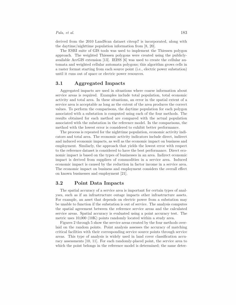
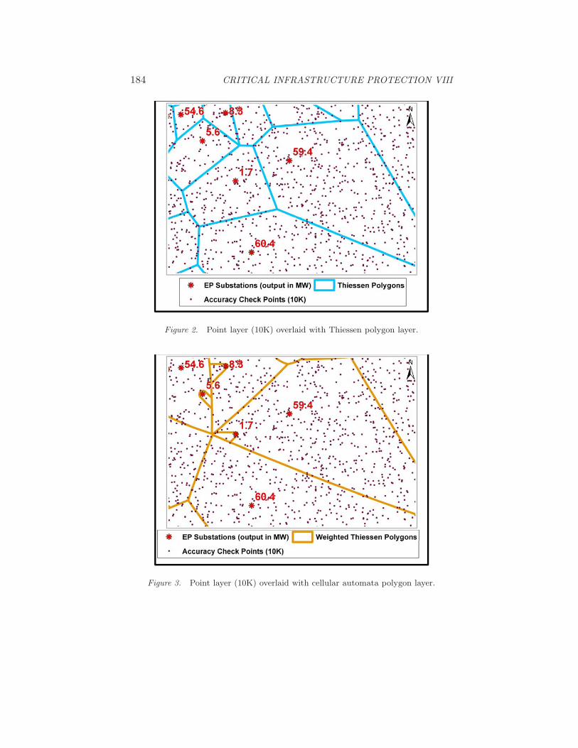
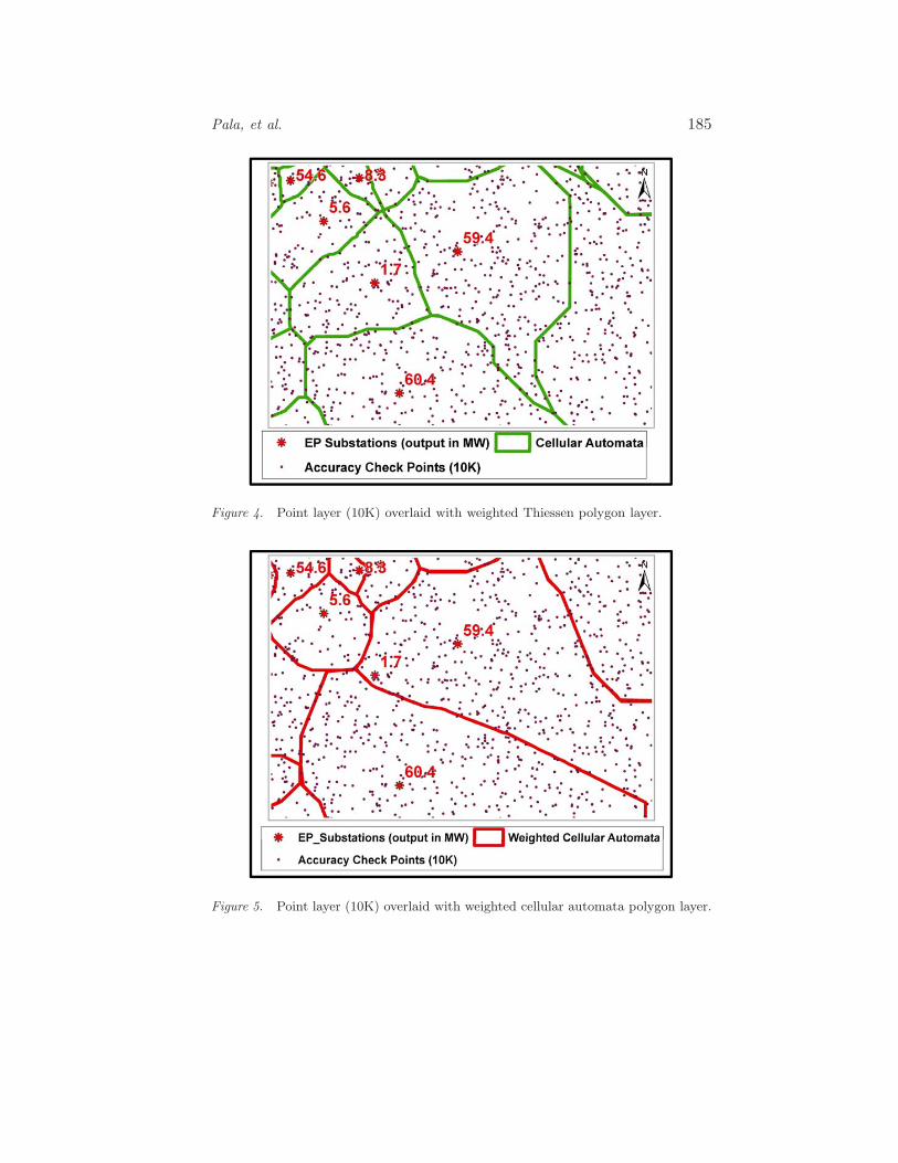
Figures 2 through 5 show the service areas created by the four methods over-laid on the random points. Point analysis assesses the accuracy of matchingcritical facilities with their corresponding service source points through serviceareas. This type of analysis is widely used in land cover classification accu-racy assessments [10, 11]. For each randomly-placed point, the service area towhich the point belongs in the reference model is determined; the same deter-


Figure 2. Point layer (10K) overlaid with Thiessen polygon layer.

Figure 3. Point layer (10K) overlaid with cellular automata polygon layer.

Pala, et al. 185

Figure 4. Point layer (10K) overlaid with weighted Thiessen polygon layer.

Figure 5. Point layer (10K) overlaid with weighted cellular automata polygon layer.


SA LayerThiessen(TP)

SA LayerThiessen(TP)

SA LayerWeightedThiessen(WTP)

SA LayerWeightedThiessen(WTP)

SA LayerCellularAutomata

(CA)

SA LayerCellularAutomata

(CA)

SA LayerWeightedCellularAutomata(WCA)

SA LayerWeightedCellularAutomata(WCA)

SA LayerReferenceData (Ref)

SA LayerReferenceData (Ref)

Datasetwith 10KRandomPoints

Datasetwith 10KRandomPoints

SPATIALJOIN

SPATIALJOIN

SPATIALJOIN

SPATIALJOIN

10K Points withReference Data

Attributes

10K Pointswith Refand TP

Attributes

10K Pointswith Refand TP

Attributes

10K Pointswith Refand WTPAttributes

10K Pointswith Refand WTPAttributes

10K Pointswith Refand CA

Attributes

10K Pointswith Refand CA

Attributes

10K Pointswith Refand WCAAttributes

10K Pointswith Refand WCAAttributes

ErrorMatrixfor TP

ErrorMatrixfor TP

ErrorMatrixfor WTP

ErrorMatrixfor WTP

ErrorMatrixfor CA

ErrorMatrixfor CA

ErrorMatrixfor WCA

ErrorMatrixfor WCA

Comparisonof Attributes

Figure 6. Point accuracy assessment data preparation flowchart.

mination is performed for the Thiessen polygon, weighted Thiessen polygon,cellular automata and weighted cellular automata approaches (Figure 6). Thisinformation is used to create error matrices for evaluating the approaches.

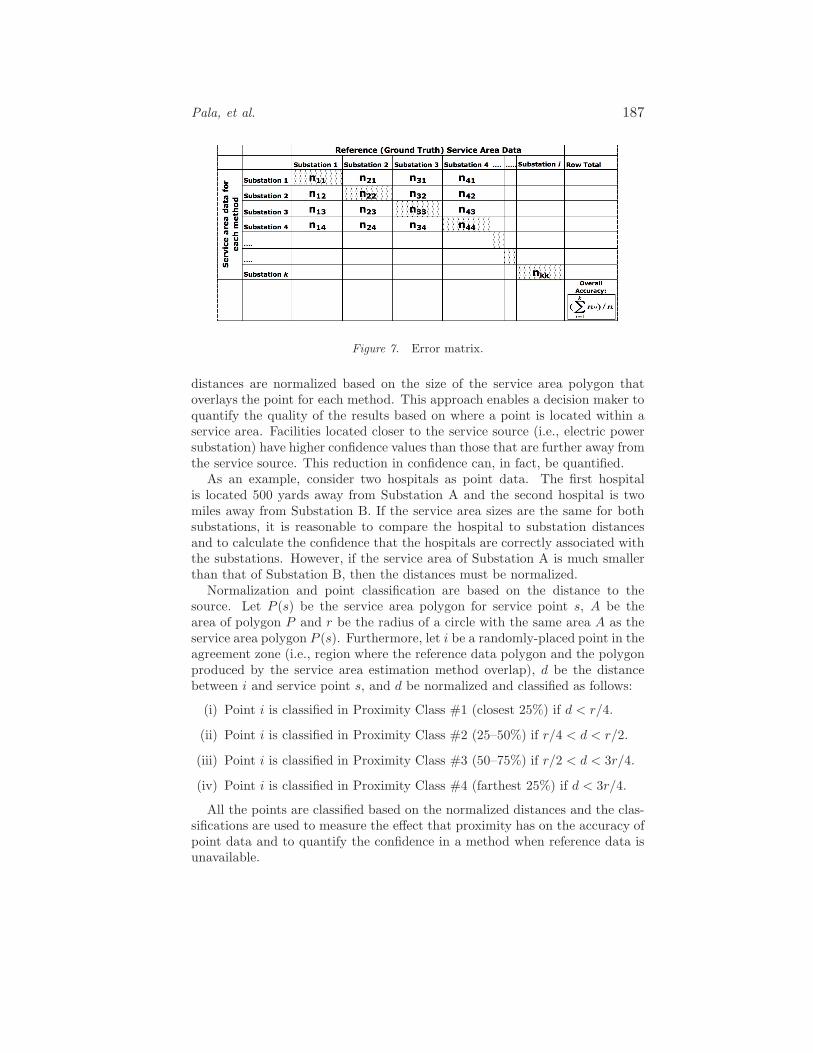
The following equation is used to extract the overall accuracy measure froman error matrix [11]:

Overall Accuracy =∑k

i=1 nii

k

where k is the number of substations, n is the number of sample points and nii

is a cell along the matrix diagonal corresponding to column i and row i.Figure 7 shows an error matrix. The columns are the reference values and the

rows are the values for a particular method (e.g., weighted cellular automata).Four such matrices are created (one for each method) to assess the accuracy ofeach calculated dataset compared with the reference dataset. For each samplepoint, the reference and calculated polygons in which the point falls (i and j,respectively) are determined. If both polygons represent the service area forthe same substation, then the ID fields match (i.e., i = j), which causes thenij cell in the matrix to be incremented by one.

Proximity confidence analyses are also performed to estimate if the proximityto the source point in a polygon affects the accuracy of the estimation. In theanalyses, the distance between the source point and the substation (defined as aserving point in the reference dataset) is measured for each polygon. To classifythe points uniformly based on their proximity to the serving source point, the

Pala, et al. 187

Figure 7. Error matrix.

distances are normalized based on the size of the service area polygon thatoverlays the point for each method. This approach enables a decision maker toquantify the quality of the results based on where a point is located within aservice area. Facilities located closer to the service source (i.e., electric powersubstation) have higher confidence values than those that are further away fromthe service source. This reduction in confidence can, in fact, be quantified.

As an example, consider two hospitals as point data. The first hospitalis located 500 yards away from Substation A and the second hospital is twomiles away from Substation B. If the service area sizes are the same for bothsubstations, it is reasonable to compare the hospital to substation distancesand to calculate the confidence that the hospitals are correctly associated withthe substations. However, if the service area of Substation A is much smallerthan that of Substation B, then the distances must be normalized.

Normalization and point classification are based on the distance to thesource. Let P (s) be the service area polygon for service point s, A be thearea of polygon P and r be the radius of a circle with the same area A as theservice area polygon P (s). Furthermore, let i be a randomly-placed point in theagreement zone (i.e., region where the reference data polygon and the polygonproduced by the service area estimation method overlap), d be the distancebetween i and service point s, and d be normalized and classified as follows:

(i) Point i is classified in Proximity Class #1 (closest 25%) if d < r/4.

(ii) Point i is classified in Proximity Class #2 (25–50%) if r/4 < d < r/2.

(iii) Point i is classified in Proximity Class #3 (50–75%) if r/2 < d < 3r/4.

(iv) Point i is classified in Proximity Class #4 (farthest 25%) if d < 3r/4.

All the points are classified based on the normalized distances and the clas-sifications are used to measure the effect that proximity has on the accuracy ofpoint data and to quantify the confidence in a method when reference data isunavailable.


(a) (b)

(c) (d)

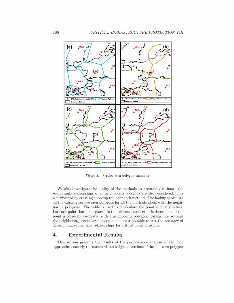
Figure 8. Service area polygon examples.

We also investigate the ability of the methods to accurately estimate thesource sink-relationships when neighboring polygons are also considered. Thisis performed by creating a lookup table for each method. The lookup table listsall the existing service area polygons for all the methods along with the neigh-boring polygons. The table is used to recalculate the point accuracy values.For each point that is misplaced in the reference dataset, it is determined if thepoint is correctly associated with a neighboring polygon. Taking into accountthe neighboring service area polygons makes it possible to test the accuracy ofdetermining source-sink relationships for critical point locations.

4. Experimental ResultsThis section presents the results of the performance analysis of the four

approaches, namely the standard and weighted versions of the Thiessen polygon

Pala, et al. 189

Table 1. Mean differences in populations.

Estimation Daytime NighttimeApproach Population Population

Thiessen Polygons 2,640 3,754Weighted Thiessen Polygons 2,554 3,505Cellular Automata 3,189 4,847Weighted Cellular Automata 1,754 541

and cellular automata approaches. For the weighted methods, peak energyconsumption (in MW) is used for the weights.

Figure 8 shows the results obtained for the four approaches. Each sub-figuredisplays one service area creation method along with the reference dataset.Figure 8(a) compares the Thiessen polygon approach results with the referenceset while Figure 8(b) compares the weighted Thiessen polygon approach resultswith the reference set. Figures 8(c) and 8(d) show the corresponding results forthe cellular automata and weighted cellular automata approaches, respectively.

The first set of results pertains to aggregate statistic accuracy analysis. Inparticular, the area, population and various economic indicators are comparedwith the results of the reference service areas.

Table 1 shows the mean differences in the daytime and nighttime populationsbetween the calculated and reference service areas. A smaller value is a betterresult because the population value produced by the method is closer to thepopulation value produced for the reference service area. For the daytime andnighttime populations, the weighted cellular automata approach yields the bestresults (smallest differences) compared with the reference data. On the otherhand, the cellular automata approach yields results with the highest differences.

Table 2. Sum of differences in populations.

Estimation Daytime NighttimeApproach Population Population

Thiessen Polygons 319K 367KWeighted Thiessen Polygons 286K 326KCellular Automata 376K 417KWeighted Cellular Automata 79K 24K

Similar results were obtained for the cumulative sum of differences in pop-ulations (Table 2). The weighted cellular automata approach yields the bestresults. The weighted Thiessen polygon approach yields better results than thestandard Thiessen polygon and cellular automata approaches.

Tables 3 and 4 show the means of the differences in the economic impactfor various metrics (direct, indirect, induced, employment and business). In allcases, the difference is smallest for the weighted cellular automata approach,


Table 3. Mean differences in economic impact (direct, indirect and induced).

Estimation Direct Indirect InducedApproach (dollars) (dollars) (dollars)

Thiessen Polygons 1.07M 1.54M 2.12MWeighted Thiessen Polygons 533K 707K 952KCellular Automata 330K 448K 611KWeighted Cellular Automata 11K 8K 16K

Table 4. Mean differences in economic impact (employment and business).

Estimation Employment BusinessApproach (dollars) (dollars)

Thiessen Polygons 6,200 560Weighted Thiessen Polygons 2,700 80Cellular Automata 1,900 200Weighted Cellular Automata 250 10

second smallest for the cellular automata approach and third smallest for theweighted Thiessen polygon approach. The only exception is the economic im-pact on business (Figure 12), for which the weighted Thiessen polygon approachand cellular automata approach swap places. The largest mean difference valueis produced by the Thiessen polygon approach. Although the mean differencefor the weighted Thiessen polygon approach is larger than that for the cellularautomata approach (with the exception of economic impact on business), thedifferences are not as notable as the differences for the other categories.

Table 5. Total sum of differences in economic impact (direct, indirect and induced).

Estimation Direct Indirect InducedApproach (dollars) (dollars) (dollars)

Thiessen Polygons 59M 85M 116MWeighted Thiessen Polygons 25M 33M 44KCellular Automata 16M 22M 31MWeighted Cellular Automata 500K 360K 714K

Tables 5 and 6 show the results corresponding to the sums of the differences;the results have the same trends as in the case of the mean differences.

The final aggregate statistic comparison considers the total surface area ofthe polygons. The results for the total surface area comparisons indicate thatthe average reference polygon area is 1,033 square acres. As shown in Table 7,the weighted cellular automata and Thiessen polygon approaches yield polygonsthat are the closest in size (on average) to the reference polygon sizes. The

Pala, et al. 191

Table 6. Total sum of differences in economic impact (employment and business).

Estimation Employment BusinessApproach (dollars) (dollars)

Thiessen Polygons 340K 31KWeighted Thiessen Polygons 127K 4KCellular Automata 96K 11KWeighted Cellular Automata 6.4K 0.5K

Table 7. Average service area polygon size.

Estimation Mean RMSApproach (acres) (acres)

Reference Data 1,033 2,241Thiessen Polygons 1,054 2,145Weighted Thiessen Polygons 1,106 2,536Cellular Automata 898 1,822Weighted Cellular Automata 921 2,299

cellular automata approach yields the least accurate approximation for thismetric.

Table 8. Overall accuracy through point analysis.

Estimation AcccuracyApproach (%)

Thiessen Polygons 54.1Weighted Thiessen Polygons 68.9Cellular Automata 52.3Weighted Cellular Automata 59.5

For the point accuracy analysis, 10,000 points were selected randomly acrossthe study area and an error matrix was created for each method. The matriceswere used to calculate the overlay agreement accuracy. Table 8 shows that theweighted Thiessen polygon approach yields the best overall results (68.9%),followed by the weighted cellular polygon approach (59.5%), while the cellularautomata approach has the least accuracy (52.3%).

As shown in Table 9, the results are nuanced. The weighted Thiessen polygonapproach has the highest point accuracy (91%) when points in the closest 25%area of each polygon are considered, followed by the weighted Thiessen poly-gon approach (86%), the cellular automate approach (85%) and the Thiessenpolygon approach (81%). Farther away from the source point, a drop in the ac-curacy of the unweighted approaches (Thiessen polygon and cellular automata)


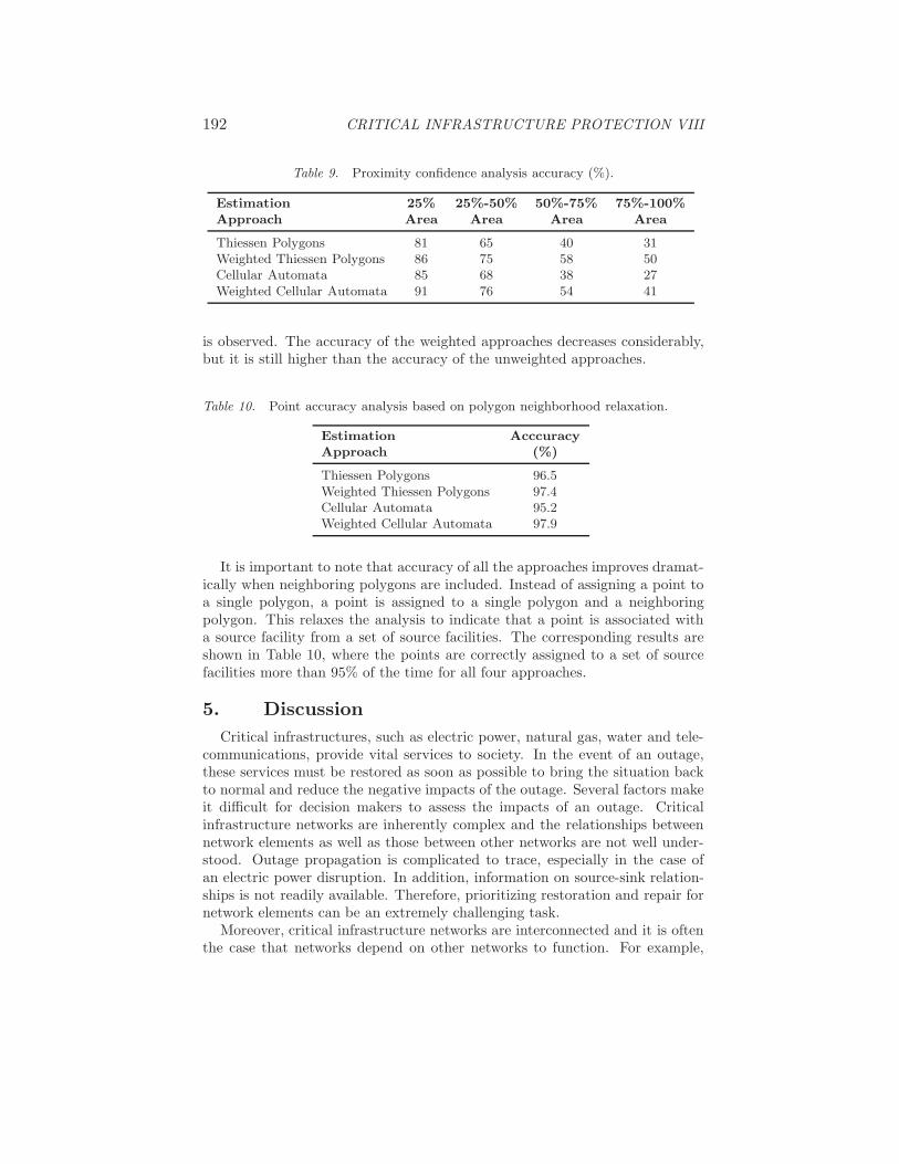
Table 9. Proximity confidence analysis accuracy (%).

Estimation 25% 25%-50% 50%-75% 75%-100%Approach Area Area Area Area

Thiessen Polygons 81 65 40 31Weighted Thiessen Polygons 86 75 58 50Cellular Automata 85 68 38 27Weighted Cellular Automata 91 76 54 41

is observed. The accuracy of the weighted approaches decreases considerably,but it is still higher than the accuracy of the unweighted approaches.

Table 10. Point accuracy analysis based on polygon neighborhood relaxation.

Estimation AcccuracyApproach (%)

Thiessen Polygons 96.5Weighted Thiessen Polygons 97.4Cellular Automata 95.2Weighted Cellular Automata 97.9

It is important to note that accuracy of all the approaches improves dramat-ically when neighboring polygons are included. Instead of assigning a point toa single polygon, a point is assigned to a single polygon and a neighboringpolygon. This relaxes the analysis to indicate that a point is associated witha source facility from a set of source facilities. The corresponding results areshown in Table 10, where the points are correctly assigned to a set of sourcefacilities more than 95% of the time for all four approaches.

5. DiscussionCritical infrastructures, such as electric power, natural gas, water and tele-

communications, provide vital services to society. In the event of an outage,these services must be restored as soon as possible to bring the situation backto normal and reduce the negative impacts of the outage. Several factors makeit difficult for decision makers to assess the impacts of an outage. Criticalinfrastructure networks are inherently complex and the relationships betweennetwork elements as well as those between other networks are not well under-stood. Outage propagation is complicated to trace, especially in the case ofan electric power disruption. In addition, information on source-sink relation-ships is not readily available. Therefore, prioritizing restoration and repair fornetwork elements can be an extremely challenging task.

Moreover, critical infrastructure networks are interconnected and it is oftenthe case that networks depend on other networks to function. For example,

Pala, et al. 193

an electric network provides power to water pumps, which are part of a waternetwork. Likewise, telecommunications towers and hubs also require electricityto function. Therefore, an outage in an electric power network can cascadewithin the network as well as to other networks. The accurate determinationof service areas is vital to modeling cross-infrastructure effects. Applying fourwell-known estimation methods, namely standard and weighted Thiessen poly-gon and cellular automata approaches, to service area determination for electricpower networks yields interesting insights. In general, the weighted cellular au-tomata approach is the best performer while the Thiessen polygon approachhas the worst performance. However, for points closest to the boundaries ofservice areas, the weighted Thiessen polygon approach has the best accuracy.

Visual inspection of the weighted cellular automata polygons compared withthe reference dataset polygons provides some insights into the point accuracyresults. Two situations lead to the lower accuracy of weighted cellular automatapolygons in the point accuracy analysis. The first involves weighted cellularautomata polygons at the outer edge of the study area and is an artifact of howa cellular automata algorithm is designed. Cellular automata algorithms favorgrowth in unconstrained regions and, thus, polygons at the edges tend to growoutward rather than inward, leading to unrealistic results. This behavior canbe controlled by introducing boundaries that limit cellular automata growth.The second situation occurs for a few cases in the dataset where the ratio ofpower output for a specific substation to the total service area in the referencedataset is too large (e.g., when some of the power is provided to an industrialcomplex). Including substations with large outputs and small area coverage inthe reference dataset also contributes to errors.

Finally, cellular automata algorithms incorporate several parameters thatmust be tuned. This study has used “out of the box” parameters for cellu-lar automata to allow for the least-biased comparisons with Thiessen polygonapproaches. However, while parameter tuning can dramatically improve theperformance of cellular automata approaches, the tuning is highly specific tothe application domain.

6. ConclusionsSophisticated modeling and simulation tools are vital to enable decision mak-

ers to predict, plan for and respond to complex critical infrastructure serviceoutages [27, 37]. However, modeling and simulation tools cannot function ef-fectively without adequate, good-quality data. Unfortunately, data pertainingto critical infrastructure assets is highly sensitive and is, therefore, difficult toobtain; detailed data about infrastructure dependencies is even more difficultto obtain.

Absent data of adequate quantity and quality, the only feasible solution isto rely on estimation methods to predict the impacts of critical infrastruc-ture service outages on populations, regional economies and other critical in-frastructure components. The empirical evaluation of service area estimationtechniques described in this paper reveals that the weighted cellular automata


and weighted Thiessen polygon approaches produce better estimates than theirstandard (unweighted) counterparts. Also, the results demonstrate that theweighted cellular automata approach has the best aggregate statistic accuracywhile the weighted Thiessen polygon approach has the best point accuracy.However, parameter tuning dramatically improves the performance of the cel-lular automata approach.

Future research will proceed along three directions. First, other criticalinfrastructures will be investigated to gain an understanding of the aspectsthat are unique to critical infrastructures and those that are common betweencritical infrastructures. Second, develop other comparison metrics with be de-veloped; for example, substation loads (in MW) could be compared with theexpected consumption of the population and businesses in service areas to as-sess the accuracy of the computed polygons. Third, formal probability-basedmethods will be investigated to cope with the error and uncertainty that un-derlie service area algorithms.

References

[1] K. Akabane, K. Nara, Y. Mishima and K. Tsuji, Optimal geographic al-location of power quality control centers by Voronoi diagram, Proceedingsof the Power Systems Computation Conference, 2002.

[2] F. Aurenhammer, Voronoi diagrams: A survey of a fundamental geometricdata structure, ACM Computing Surveys, vol. 23(3), pp. 345–405, 1991.

[3] A. Barto, Cellular Automata as Models of Natural Systems, Ph.D. Disser-tation, Department of Computer and Communication Sciences, Universityof Michigan, Ann Arbor, Michigan, 1975.

[4] F. Berto and J. Tagliabue, Cellular automata, in The Stanford Encyclope-dia of Philosophy, E. Zalta (Ed.), Stanford, California (plato.stanford.edu/archives/sum2012/entries/cellular-automata), 2012.

[5] E. Bright, P. Coleman and A. Rose, LandScan 2011 Global PopulationDatabase, Oak Ridge National Laboratory, Oak Ridge, Tennessee, 2012.

[6] B. Bush, A. Bush, R. Fisher, S. Folga, P. Giguere, J. Holland, J. Hur-ford, J. Kavicky, A. McCown, M. McLamore, E. Pontante, L. Rothrock,M. Salazar, S. Shamsuddin, C. Unal, D. Visarraga and K. Werley, In-terdependent Energy Infrastructure Simulation System – IEISS Version2.1 Technical Reference Manual, Technical Report LANL-D4-05-0027, LosAlamos National Laboratory, Los Alamos, New Mexico, 2005.

[7] S. Castongia, A Demand-Based Resource Allocation Method for Electri-cal Substation Service Area Delineation, M.A. Thesis, Department of Ge-ography and Earth Sciences, University of North Carolina at Charlotte,Charlotte, North Carolina, 2006.

[8] J. Ching, M. Brown, T. McPherson, S. Burian, F. Chen, R. Cionco, A.Hanna, T. Hultgren, D. Sailor, H. Taha and D. Williams, National Urban

Pala, et al. 195

Database and Access Portal Tool, Bulletin of the American MeteorologicalSociety, vol. 90(8), pp. 1157–1168, 2009.

[9] B. Chopard, Cellular automata modeling of physical systems, in Computa-tional Complexity: Theory, Techniques and Applications, R. Meyers (Ed.),Springer, New York, pp. 407–433, 2012.

[10] R. Congalton, A review of assessing the accuracy of classifications of re-motely sensed data, Remote Sensing of Environment, vol. 37(1), pp. 35–46,1991.

[11] R. Congalton and K. Green, Assessing the Accuracy of Remotely SensedData: Principles and Practices, CRC Press, Boca Raton, Florida, 2009.

[12] M. Creutz, Self-organized criticality and cellular automata, in Computa-tional Complexity: Theory, Techniques and Applications, R. Meyers (Ed.),Springer, New York, pp. 2780–2791, 2012.

[13] P. Dong, Generating and updating multiplicatively weighted Voronoi di-agrams for point, line and polygon features in GIS, Computers and Geo-sciences, vol. 34(4), pp. 411–421, 2008.

[14] J. Fenwick and L. Dowell, Electrical substation service-area estimationusing cellular automata: An initial report, Proceedings of the ACM Sym-posium on Applied Computing, pp. 560–565, 1999.

[15] M. Gahegan and I. Lee, Data structures and algorithms to support in-teractive spatial analysis using dynamic Voronoi diagrams, Computers,Environment and Urban Systems, vol. 24(6), pp. 509–537, 2000.

[16] M. Held and R. Williamson, Creating electrical distribution boundariesusing computational geometry, IEEE Transactions on Power Systems, vol.19(3), pp. 1342–1347, 2004.

[17] H. Kuo and Y. Hsu, Distribution system load estimation and servicerestoration using a fuzzy set approach, IEEE Transactions on Power De-livery, vol. 8(4), pp. 1950–1957, 1993.

[18] S. Linger and M. Wolinsky, Estimating electrical service areas using GISand cellular automata, presented at the Environmental Systems ResearchInstitute International Conference, 2001.

[19] T. McPherson and S. Burian, The Water Infrastructure Simulation Envi-ronment (WISE) Project, Proceedings of the Seventh Annual Symposoumon Water Distribution Systems Analysis, 2005.

[20] T. McPherson, J. Rush, H. Khalsa, A. Ivey and M. Brown, A day-nightpopulation exchange model for better exposure and consequence manage-ment assessments, Proceedings of the Sixth Symposium on Urban Develop-ment, 2006.

[21] National Infrastructure Simulation and Analysis Center, FastEcon ToolSummary Report: Fiscal Year 2008, Technical Report LA-UR-09-00558,Los Alamos National Laboratory, Los Alamos, New Mexico, 2008.


[22] K. Newton and D. Schirmer, On the methodology of defining substationspheres of influence within an electric vehicle project framework, presentedat the Environmental Systems Research Institute User Conference, 1997.

[23] A. Okabe, B. Boots, K. Sugihara and S. Chiu, Spatial Tessellations:Concepts and Applications of Voronoi Diagrams, John Wiley, Chichester,United Kingdom, 2000.

[24] A. Okabe, T. Satoh, T. Furuta, A. Suzuki and K. Okano, Generalizednetwork Voronoi diagrams: Concepts, computational methods and appli-cations, International Journal of Geographical Information Science, vol.22(9), pp. 965–994, 2008.

[25] L. Sulewski, A Geographic Modeling Framework for Assessing CriticalInfrastructure Vulnerability: Energy Infrastructure Case Study, Ph.D.Dissertation, Department of Geography, University of South Carolina,Columbia, South Carolina, 2013.

[26] W. Tobler, Cellular geography, in Philosophy in Geography, S. Gale and G.Olsson (Eds.), Springer, Dordrecht, The Netherlands, pp. 379–386, 1979.

[27] W. Tolone, D. Wilson, A. Raja, W. Xiang, H. Hao, S. Phelps and E. John-son, Critical infrastructure integration modeling and simulation, Proceed-ings of the Second Symposium on Intelligence and Security Informatics,pp. 214–225, 2004.

[28] G. Toole, S. Linger and M. Burks, Automated utility service area assess-ment under emergency conditions, Proceedings of International Conferenceof the Society for Computer Simulation, 2001.

[29] P. Torrens, Cellular automata, in International Encyclopedia of HumanGeography, R. Kitchen and N. Thrift (Eds.), Elsevier, London, UnitedKingdom, pp. 1–4, 2009.

[30] P. Torrens and I. Benenson, Geographic automata systems, InternationalJournal of Geographical Information Science, vol. 19(4), pp. 385–412, 2005.

[31] P. Torrens and A. Nara, Modeling gentrification dynamics: A hybrid ap-proach, Computers, Environment and Urban Systems, vol. 31(3), pp. 337–361, 2007.

[32] P. Torrens and D. O’Sullivan, Cellular automata and urban simulation:Where do we go from here? Environment and Planning B: Planning andDesign, vol. 28(2), pp. 163–168, 2001.

[33] D. Visarraga, B. Bush, S. Linger and T. McPherson, Development of a Javabased water distribution simulation capability for infrastructure interde-pendency analyses, Proceedings of the World Water and EnvironmentalResources Congress, 2005.

[34] J. von Neumann, The Computer and the Brain, Yale University Press, NewHaven, Connecticut, 1958.

[35] J. von Neumann, Papers of John von Neumann on Computers and Com-puting Theory, MIT Press, Cambridge, Massachusetts, 1986.

Pala, et al. 197

[36] J. von Neumann and O. Morgenstern, Theory of Games and EconomicBehavior, Princeton University Press, Princeton, New Jersey, 1953.

[37] D. Wilson, O. Pala, W. Tolone and W. Xiang, Recommendation-basedgeovisualization support for reconstitution in critical infrastructure pro-tection, SPIE Proceedings on Visual Analytics for Homeland Defense andSecurity, vol. 7346, 2009.

[38] S. Wolfram, Cellular Automata and Complexity: Collected Papers, West-view Press, Boulder, Colorado, 1994.

accuracy of service area estimation …public.lanl.gov/rbent/cipbook14.pdfchapter 12 accuracy of...

Documents