Estimation of Parameters and Variance

Dr. A.C. Kulshreshtha U.N. Statistical Institute for Asia and the Pacific (SIAP)

Second RAP Regional Workshop on

Building Training Resources for Improving Agricultural & Rural Statistics Sampling Methods for Agricultural Statistics-Review of Current Practices

SCI, Tehran, Islamic Republic of Iran 10-17 September 2013

2

Estimation of Parameters

Survey Objectives: Are usually met by producing estimates of

parameters of survey variable(s) – (Population) Mean – (Population) Total – (Population) Proportion – (Population) Ratio, Regression, correlation

Which estimates are produced depends on the objectives of the survey – Your examples

3

Two aspects of sampling theory

Sample selection through Sampling Design Estimation of Parameters and their Properties

– Efficiency: provide estimates at lowest cost and reasonable enough precision

– Sampling distribution: precision of estimators are judged by the frequency distribution generated for the estimate if the sampling procedure is applied repeatedly to the same population

4

Estimator is… a function (formula) of observations by which

an estimate of some population characteristic (parameter), say, population mean is calculated from the sample

a random variable and is defined on a random sample. Each random sample will yield one of its possible values

Estimation of Parameters

5

SRS- Providing Estimator

Estimator of Population Mean, is

Where: yi = sample response for variable y, unit i; n is sample size

Y ∑=

==n

iiy

nyY

1

1ˆ

Estimator of Population Total, Y is i

n

ii

n

iywy

nNyNY ∑∑

==

==×=11

ˆ

Where, N = population size w = base (sampling) weight for each sample unit or inflation factor

6

Sampling Distributions of Estimators

To obtain the sampling distributions of estimators, the following probability sampling mechanism is considered: – It is possible to define the set of distinct

samples which the sampling procedure is capable of selecting from the population

– This further implies that it is possible to identify units belonging to different samples

iπ

7

Sampling Distribution of Estimators (Contd.)

Each of the possible samples is assigned a known probability of selection – Out of all possible samples, a sample,

selected by a random process determined by the probability of selection

Method of computing estimate from the sample (estimator) is pre-specified

8

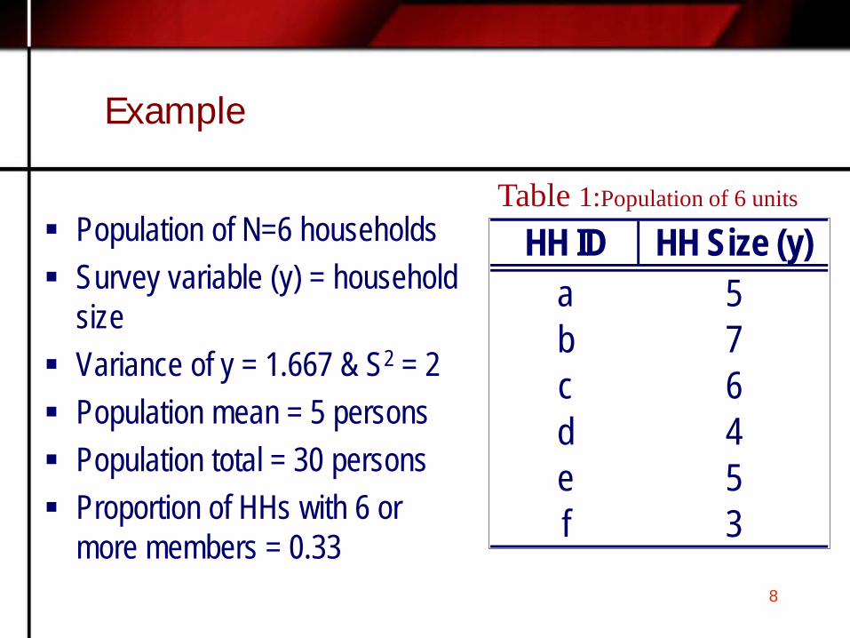
Example

Population of N=6 households Survey variable (y) = household

size Variance of y = 1.667 & S2 = 2 Population mean = 5 persons Population total = 30 persons Proportion of HHs with 6 or

more members = 0.33

HH ID HH Size (y)a 5b 7c 6d 4e 5f 3

Table 1:Population of 6 units

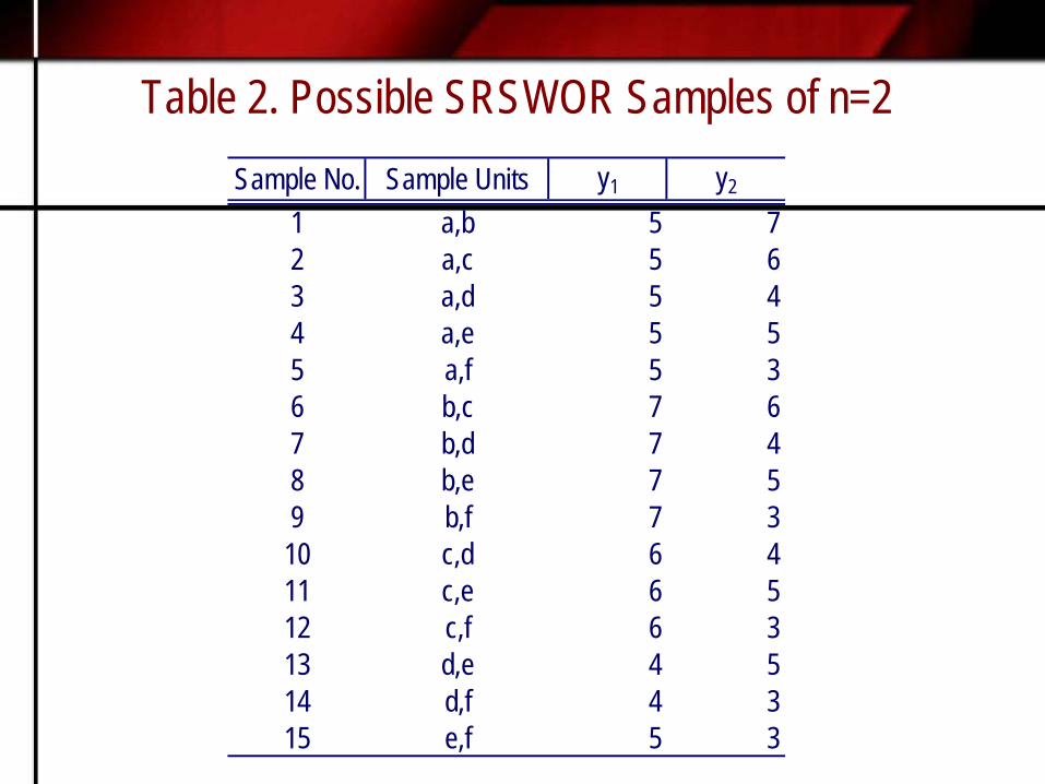
Table 2. Possible SRSWOR Samples of n=2 Sample No. Sample Units y1 y2

1 a,b 5 72 a,c 5 63 a,d 5 44 a,e 5 55 a,f 5 36 b,c 7 67 b,d 7 48 b,e 7 59 b,f 7 310 c,d 6 411 c,e 6 512 c,f 6 313 d,e 4 514 d,f 4 315 e,f 5 3

10

Show the sampling distribution of ...

sample mean sample proportion estimator of population total

11

Table 3. Estimates from Samples Sample No. y1 y2

Sample Mean

Sample Proportion

Sample Total

Sampling weight

Estimate of Population Total

1 5 7 6.0 0.5 12 3 362 5 6 5.5 0.5 11 3 333 5 4 4.5 0.0 9 3 274 5 5 5.0 0.0 10 3 305 5 3 4.0 0.0 8 3 246 7 6 6.5 1.0 13 3 397 7 4 5.5 0.5 11 3 338 7 5 6.0 0.5 12 3 369 7 3 5.0 0.5 10 3 3010 6 4 5.0 0.5 10 3 3011 6 5 5.5 0.5 11 3 3312 6 3 4.5 0.5 9 3 2713 4 5 4.5 0.0 9 3 2714 4 3 3.5 0.0 7 3 2115 5 3 4.0 0.0 8 3 24

12

Sampling Distribution of

Example, Table 3,

y

Table 4. Sampling distribution of y

13

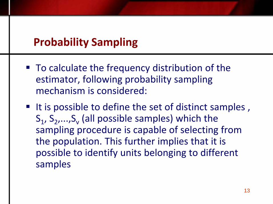
Probability Sampling

To calculate the frequency distribution of the estimator, following probability sampling mechanism is considered:

It is possible to define the set of distinct samples , S1, S2,...,Sv (all possible samples) which the sampling procedure is capable of selecting from the population. This further implies that it is possible to identify units belonging to different samples

14

Probability Sampling (Contd.)

Each of the possible sample Si is assigned a known probability of selection , say, Pi

Out of the all possible samples, a sample , Si, is selected by a random process whereby each sample Si has a probability of being selected

The method of computing estimate from the sample is pre specified

15

Probability Sampling (Contd.)

Process of generating all possible samples is laborious, particularly for large populations, thus

Procedure usually followed is – Specify inclusion probability of all the units of the

population – Select units one by one by predetermined

probabilities until sample of desired size n is selected (Random Sample)

The availability of sampling frame is a pre- requisite

Properties of Estimators

Unbiasedness Precision Accuracy

Consistency Sufficiency Efficiency

17

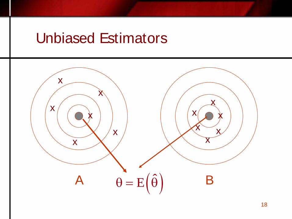
Basic Ideas: Unbiased Estimator

An estimator is an unbiased estimator for the parameter θ if the mean of its sampling distribution is equal to θ.

Bias of an estimator

θ̂

( ) ( )ˆ ˆθ 0E Eθ = ⇒ θ −θ =

( )ˆ(θ) θ̂ θEBias = −

18

Unbiased Estimators

x

x x

x

x x

A

x x

x x x

x

B ( )ˆEθ = θ

19

Biased Estimators

x

x

x x

x x

C

( ) ( ) θ−θ=θ ˆEˆBias

θ

( )ˆE θ

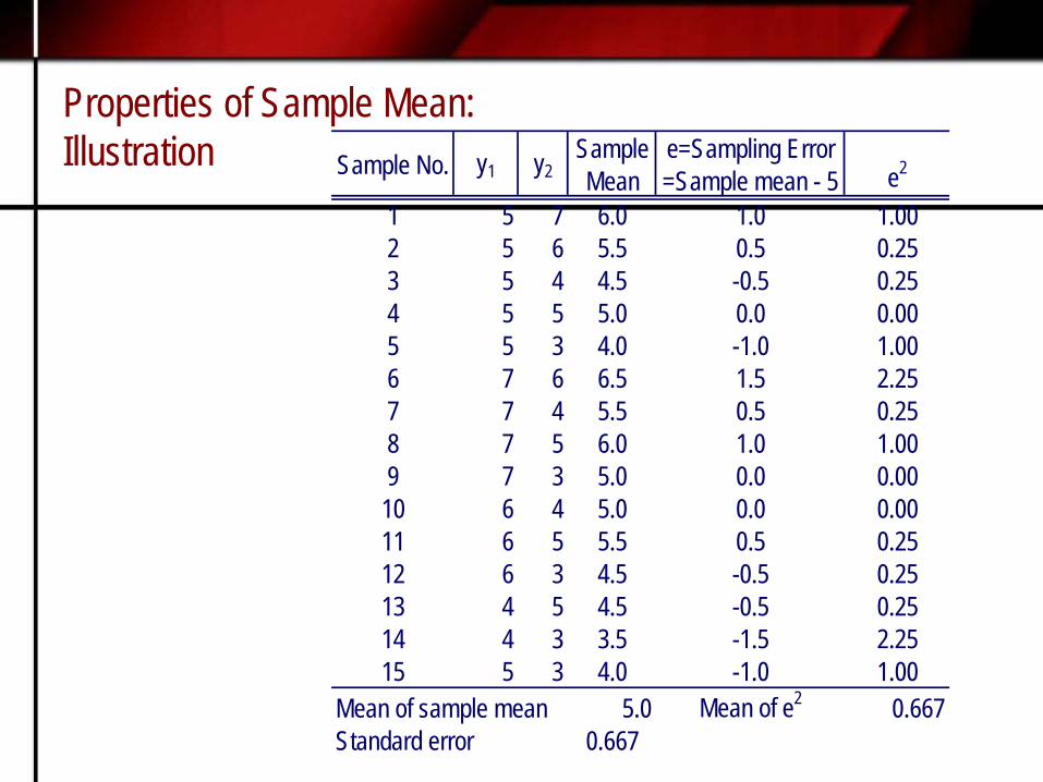
Properties of Sample Mean: Illustration Sample No. y1 y2

Sample Mean

e=Sampling Error =Sample mean - 5 e2

1 5 7 6.0 1.0 1.002 5 6 5.5 0.5 0.253 5 4 4.5 -0.5 0.254 5 5 5.0 0.0 0.005 5 3 4.0 -1.0 1.006 7 6 6.5 1.5 2.257 7 4 5.5 0.5 0.258 7 5 6.0 1.0 1.009 7 3 5.0 0.0 0.0010 6 4 5.0 0.0 0.0011 6 5 5.5 0.5 0.2512 6 3 4.5 -0.5 0.2513 4 5 4.5 -0.5 0.2514 4 3 3.5 -1.5 2.2515 5 3 4.0 -1.0 1.00

Mean of sample mean 5.0 Mean of e2 0.667Standard error 0.667

21

Sampling design SRSWR or SRSWOR

Population parameter

Sample mean is an unbiased estimator

of population mean

∑=N

iiY

NY 1

∑=n

iiy

ny 1

Example 1- Design-based Estimator

22

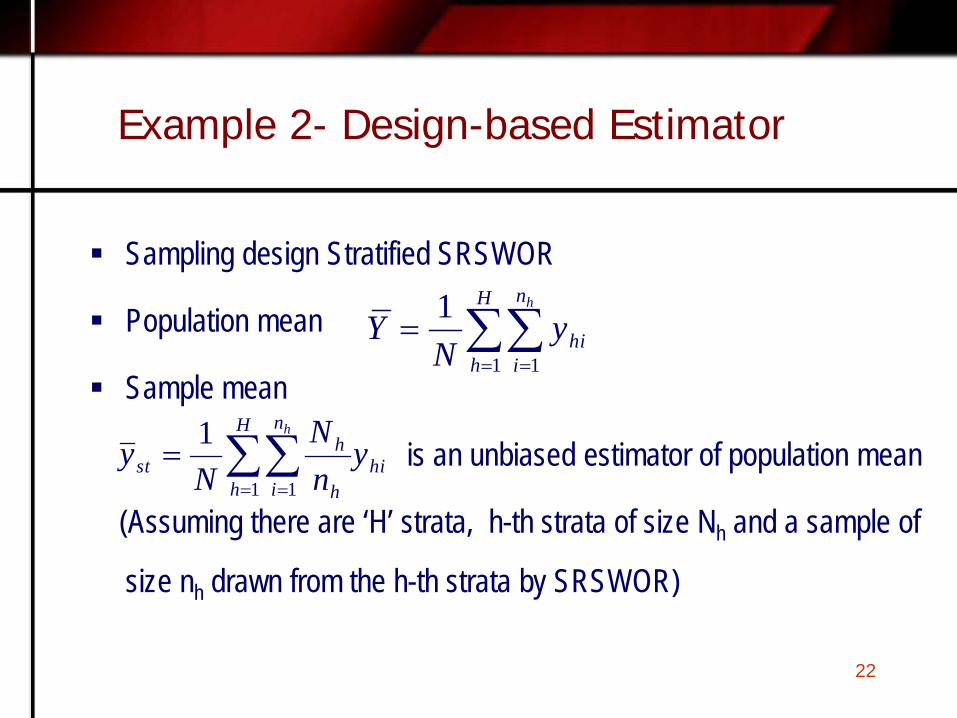
Sampling design Stratified SRSWOR

Population mean

Sample mean

is an unbiased estimator of population mean

(Assuming there are ‘H’ strata, h-th strata of size Nh and a sample of

size nh drawn from the h-th strata by SRSWOR)

Example 2- Design-based Estimator

∑∑= =

=H

h

n

ihi

h

yN

Y1 1

1

hi

H

h

n

i h

hst y

nN

Ny

h

∑∑= =

=1 1

1

23

Example 3- Ratio Estimator

Sampling design SRSWOR

Population parameter

Estimator (ratio estimator) is a biased estimator

Bias of the ratio estimator is

∑=N

iiY

NY 1

( )yxx CCCYNn

nN ρ−

− 2

XxyyY rR ==ˆ

24

Sampling Error

Sampling error of is the difference between the estimate and the parameter it is estimating

θθ̂e −=

θ̂

25

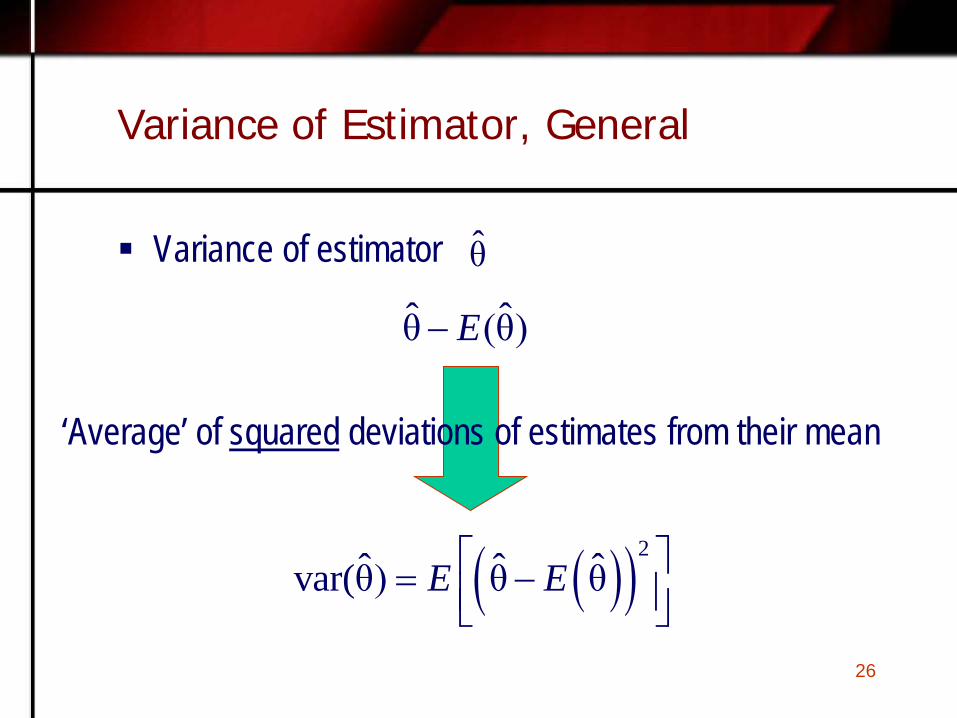
Variance of Unbiased Estimator

Variance of unbiased estimator θ̂

( )2ˆ ˆvar(θ) θ θE = −

‘Average’ of squared deviations of all possible estimates

θθ̂e −=

26

Variance of Estimator, General

Variance of estimator

ˆ ˆθ (θ)E−

θ̂

( )( )2ˆ ˆ ˆvar(θ) θ θE E = −

‘Average’ of squared deviations of estimates from their mean

27

Precise Estimators

x

x

x x

x x

C

x x x

x x

B

x

Variance is small of precise estimator Smaller the variance, more precise the estimator

28

Accurate Estimator

Which estimator is the most accurate?

x

x

x x x x

C

x x

x x x

x

B

x

x x

x x

x

A

An estimator is said to be accurate if both bias and variance are small

29

Mean Squared Error (MSE)

Total error (simple model) = ( ) ( ) θ]θ̂E[]θ̂Eθ̂[θθ̂ −+−=−

22 })ˆ(E{)]}ˆ(Eˆ{[E θ−θ+θ−θ=Variable error Bias2

2)θ̂Bias()θ̂Var()θ̂MSE( +=

Measure of accuracy is Mean Squared Error

30

Example: Ratio Estimator in SRSWOR

Population parameter

Estimator

Bias of the ratio estimator is

MSE of the ratio estimator is

∑=N

iiY

NY 1

( )yxx CCCYNn

nN ρ−

− 2

( ) ( ) 22222 2

−

−

+−+

−

yxxyxxy CCCYNn

nNCCCCYNn

nN ρρ

XxyyY rR ==ˆ

31

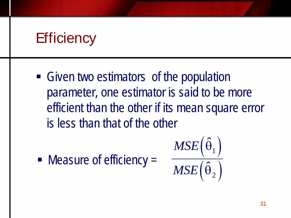
Efficiency

Given two estimators of the population parameter, one estimator is said to be more efficient than the other if its mean square error is less than that of the other

( )( )

1

2

ˆ

ˆMSE

MSE

θ

θ Measure of efficiency =

32

Consistency

An estimator is said to be a consistent estimator if its value

approaches parameter, statistically

the probability of the difference being less than

any specified small quantity tends to unity as n is increased

Also, when n is increased to ‘N’ the estimator attains the

value of the parameter

µµ −ˆ

33

Sampling design SRSWR

Population parameter

Sample mean is a consistent estimator of

the population mean

∑=N

iiY

NY 1

∑=n

iiy

ny 1

Example 1

34

Sampling design SRSWOR

Population parameter

Sample mean is a consistent

estimator of the population mean

∑=N

iiY

NY 1

∑=n

iiy

ny 1

Example 2

35

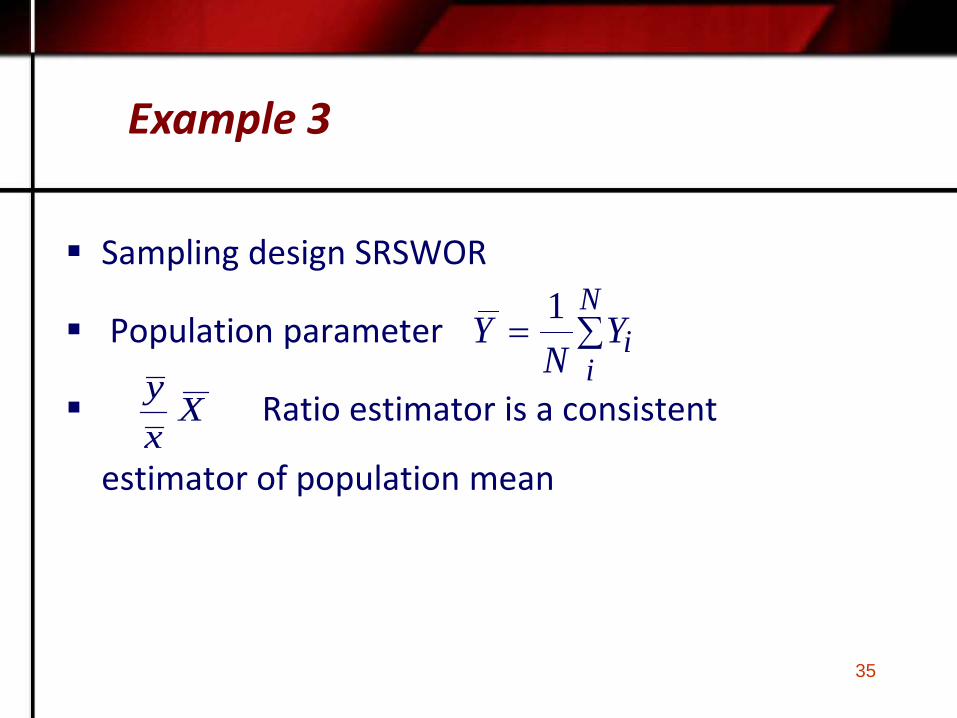
Sampling design SRSWOR

Population parameter

Ratio estimator is a consistent

estimator of population mean

∑=N

iiY

NY 1

Xxy

Example 3

36

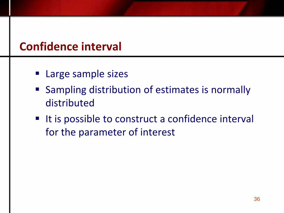
Confidence interval

Large sample sizes Sampling distribution of estimates is normally

distributed It is possible to construct a confidence interval

for the parameter of interest

37

Sampling design SRSWR

Population parameter

Sample mean

5% CI

1% CI

21196.1 SNn

Y

−±

21158.2 SNn

Y

−±

Example

∑=N

iiY

NY 1

∑=n

iiy

ny 1

38

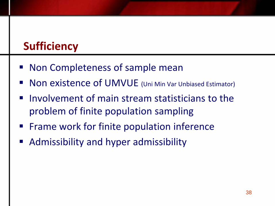
Sufficiency

Non Completeness of sample mean Non existence of UMVUE (Uni Min Var Unbiased Estimator)

Involvement of main stream statisticians to the problem of finite population sampling

Frame work for finite population inference Admissibility and hyper admissibility

39

Other approaches

Likelihood function approach Model based approach Robustness aspect Model assisted approach Use of models but inferences are design based Conditional design based approach

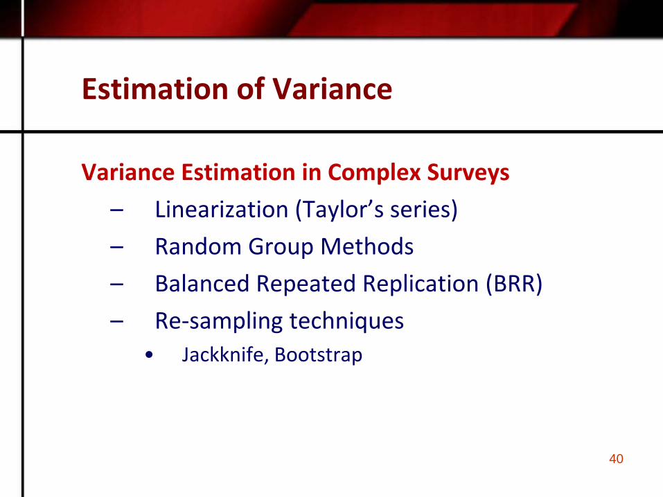
Estimation of Variance

Variance Estimation in Complex Surveys – Linearization (Taylor’s series) – Random Group Methods – Balanced Repeated Replication (BRR) – Re-sampling techniques

• Jackknife, Bootstrap

40

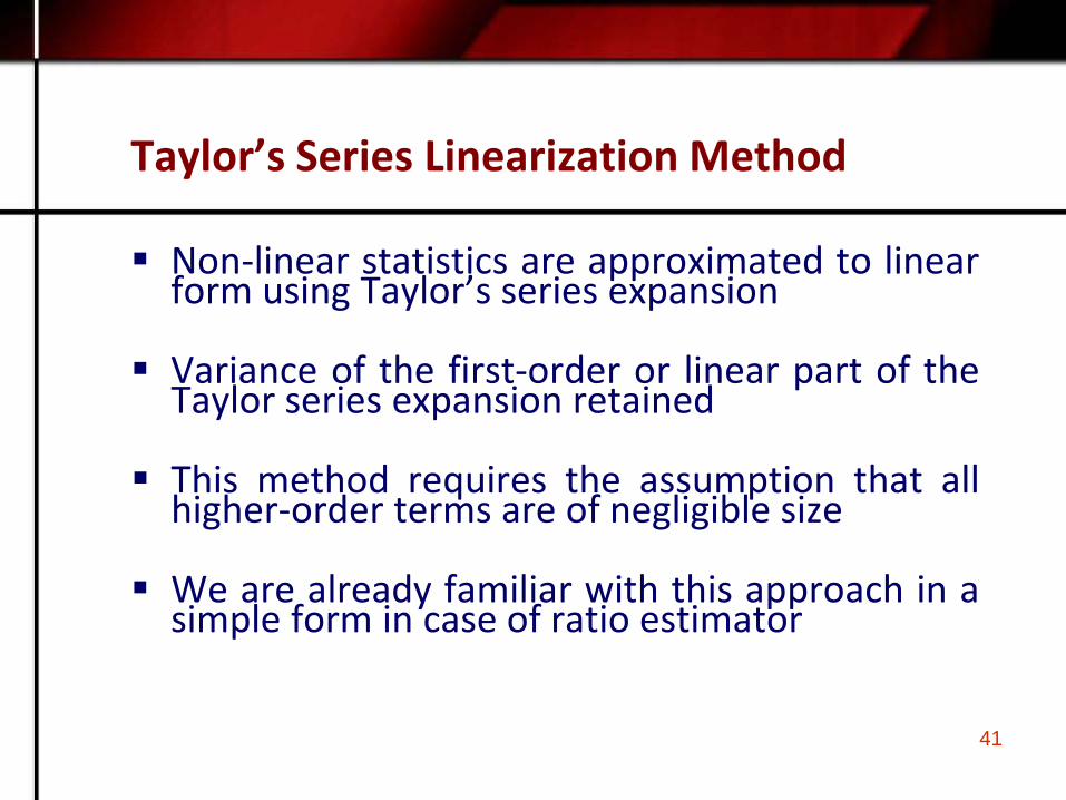
Taylor’s Series Linearization Method

Non-linear statistics are approximated to linear form using Taylor’s series expansion

Variance of the first-order or linear part of the

Taylor series expansion retained This method requires the assumption that all

higher-order terms are of negligible size We are already familiar with this approach in a

simple form in case of ratio estimator

41

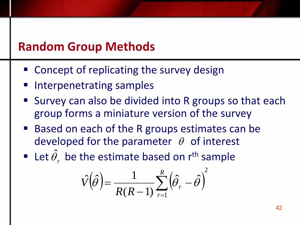
Random Group Methods

Concept of replicating the survey design Interpenetrating samples Survey can also be divided into R groups so that each

group forms a miniature version of the survey Based on each of the R groups estimates can be

developed for the parameter of interest Let be the estimate based on rth sample

θ

rθ̂

( ) ( )2

1

ˆˆ)1(

1ˆˆ ∑=

−−

=R

rrRR

V θθθ

42

BRR method

Consider that there are H strata with two units selected per stratum

There are ways to pick 1 from each stratum Each combination could be treated as a sample Pick R samples Which samples should we include?

H2

43

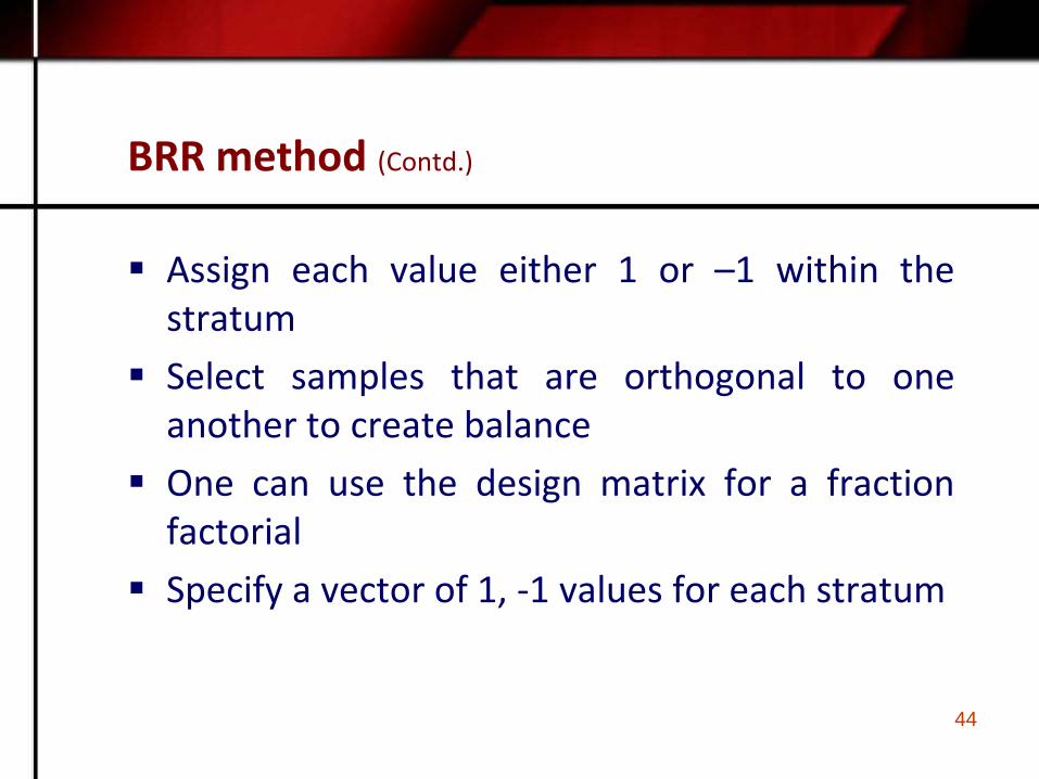
BRR method (Contd.)

Assign each value either 1 or –1 within the stratum

Select samples that are orthogonal to one another to create balance

One can use the design matrix for a fraction factorial

Specify a vector of 1, -1 values for each stratum

44

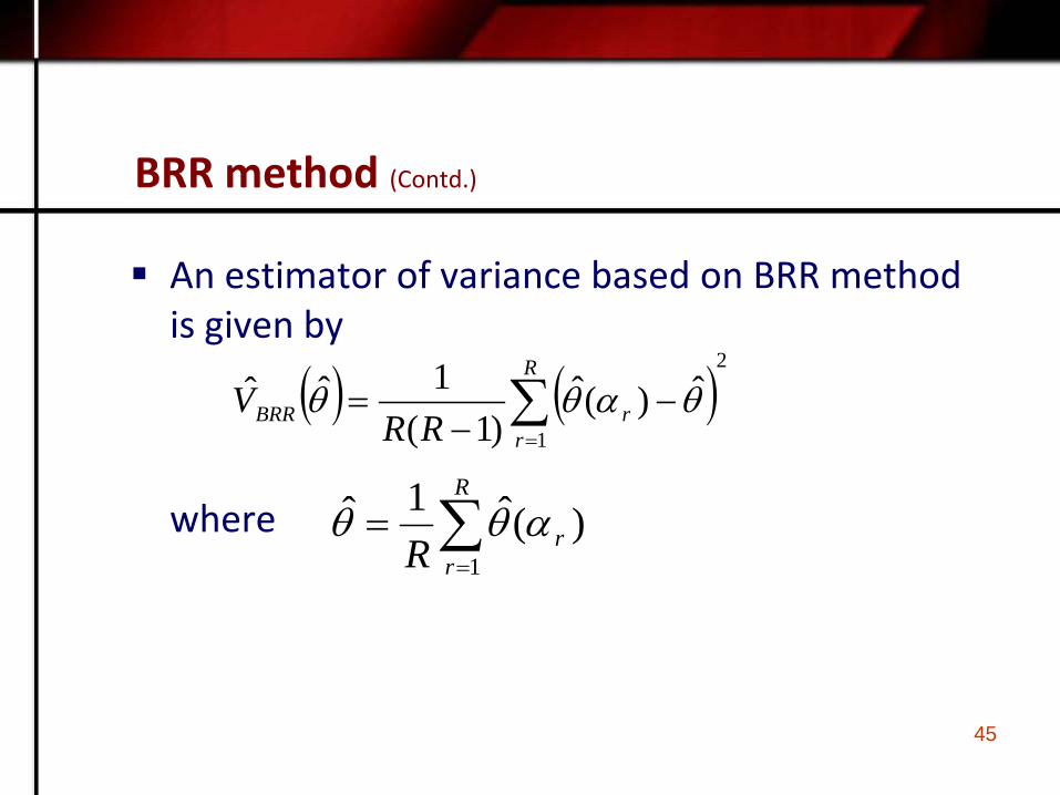
BRR method (Contd.)

An estimator of variance based on BRR method is given by

where

( ) ( )2

1

ˆ)(ˆ)1(

1ˆˆ ∑=

−−

=R

rrBRR RR

V θαθθ

∑=

=R

rrR 1)(ˆ1ˆ αθθ

45

Jack-knife Method

Let be the estimator of θ after omitting the ith observation. Define

iθ̂

ii nn θθθ ˆ)1(ˆ~−−=

∑= iJ n

θθ ~1ˆ

∑=

−−

=n

iJ

iJJ nn

V1

2)ˆ~()1(

1)ˆ(ˆ θθθ

46

Soft-wares for Variance estimation

OSIRIS – BRR, Jackknife SAS – Linearization STATA – Linearization SUDAAN – Linearization, Bootstrap, Jackknife WesVar – BRR, Jackknife, Bootstrap

47

48

THANKS