Lecture 10 Image restoration and reconstruction

1 Basic concepts about image degradation/restoration1. Basic concepts about image degradation/restoration2. Noise models3 Spatial filter techniques for restoration3. Spatial filter techniques for restoration

Image Restoration

• Image restoration is to recover an image that has been degraded by using a priori knowledge of the degradation hphenomenon

• Image enhancement vs image restoration• Image enhancement vs. image restoration– Enhancement is for vision– Restoration is to recover the original image– There is overlap of the techniques used

• Image restored is an approximation of the original imageImage restored is an approximation of the original image– Criteria for the goodness

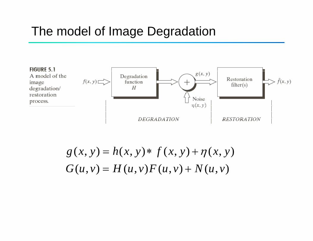
The model of Image Degradation

( , ) ( , ) ( , ) ( , )( ) ( ) ( ) ( )

g x y h x y f x y x yG H F N

η= ∗ +( , ) ( , ) ( , ) ( , )G u v H u v F u v N u v= +

Noise models

• Noise often arise during image acquisition/transformation– Caused by many factors– Spatial noise– Frequency noise

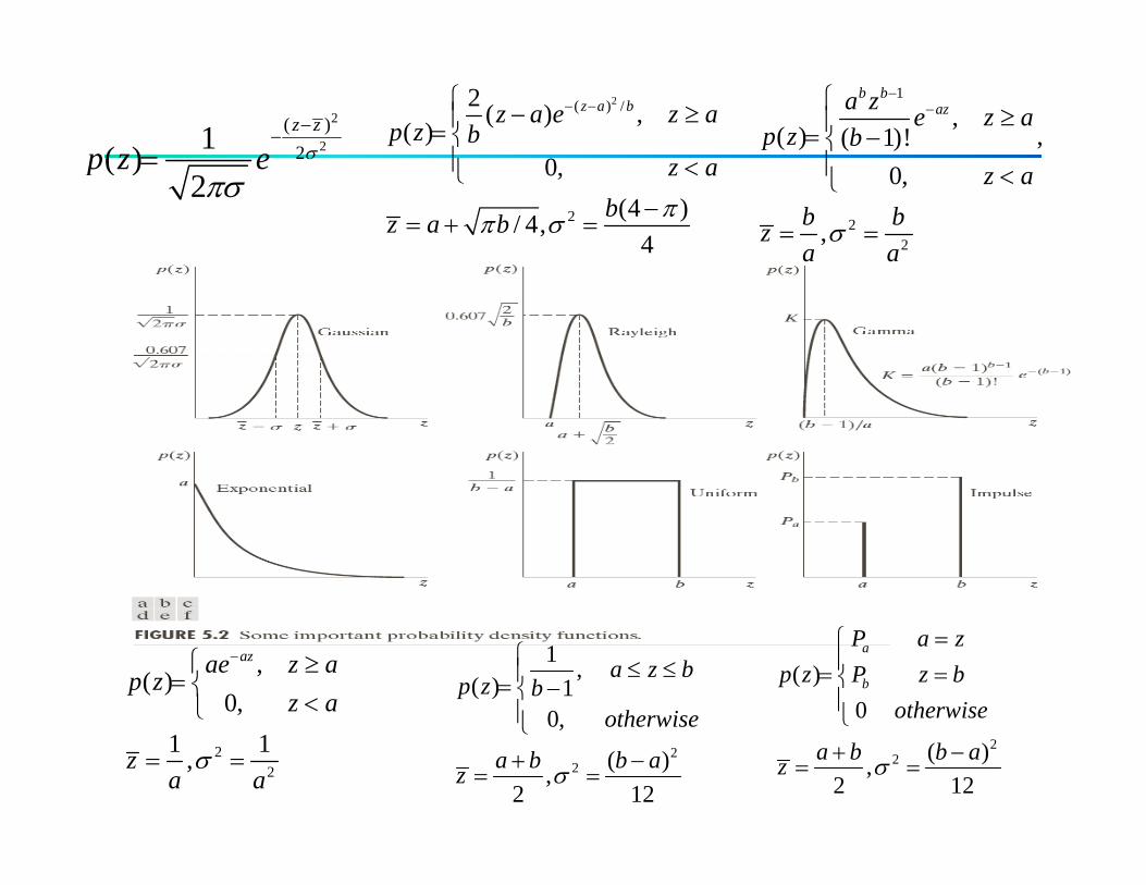
• Some important noise probability density functionsSome important noise probability density functions– Gaussian noise– Rayleigh noise

E l ( ) i– Erlang (gamma) noise– Exponential noise– Uniform– Impulse

• Periodic noise

2

2( )

21( )z z

p z e σ−

−=

2( ) /2 ( ) ,( )

0

z a bz a e z ap z b

− −⎧ − ≥⎪= ⎨⎪ <⎩

1

,( ) ,( 1)!

b baza z e z a

p z b

−−⎧

≥⎪= −⎨⎪( )

2p z e

πσ=

2

0,(4 )/ 4,

4

z abz a b ππ σ

⎪ <⎩−

= + = 22

0,

,

z ab bza aσ

⎪ <⎩

= =

,( )

0,

azae z ap z

z a

−⎧ ≥= ⎨

<⎩

1 ,( ) 1

0

a z bp z b

otherwise

⎧ ≤ ≤⎪= −⎨⎪⎩

( )0

a

b

P a zp z P z b

otherwise

=⎧⎪= =⎨⎪⎩

22

1 1,za aσ= = 2

2

0,

( ),2 12

otherwise

a b b az σ

⎪⎩+ −

= =2

2 ( ),2 12

a b b az σ

⎩+ −

= =

Generate spatial noise of a given distributionTheoremGiven CDF F(z). Let w be the uniform random number generator on

(0 1) Then the random number has the CDF F(z)1( )z F w−=(0,1). Then the random number has the CDF F(z)

Example: Reyleigh’s CDF is

( )zz F w=

p y g2( ) /1( )

0

z a b

ze z aF w

z a

− −⎧ − ≥⎪= ⎨<⎪⎩

ln(1 )z a b w= + − −

Matlab example: a = 50, b =10, M = 100, N = 100;R = a + sqrt(-b*log(1-rand(M,N)));

MatLab example 2: Gaussian distribution mean a and std bMatLab example 2: Gaussian distribution mean a and std ba = 10, b =10, M = 100, N = 100;R = a + b*randn(M,N);

Add spatial noise to an image of

• Let f(x, y) be an M N image, and N(x, y) be the random MN noise of the given distribution. Then the image with th ti l i i ( ) f( ) + N( )the spatial noise is g(x, y) = f(x,y) + N(x,y)

MatLab example: f = imread('moon.tif');[M N] = size(f);

i ( ( ( ( ))))s = uint8(a + sqrt(-b*log(1-rand(M,N))));fs = y + s;imshow(fs)

Estimation of Noise Parameters

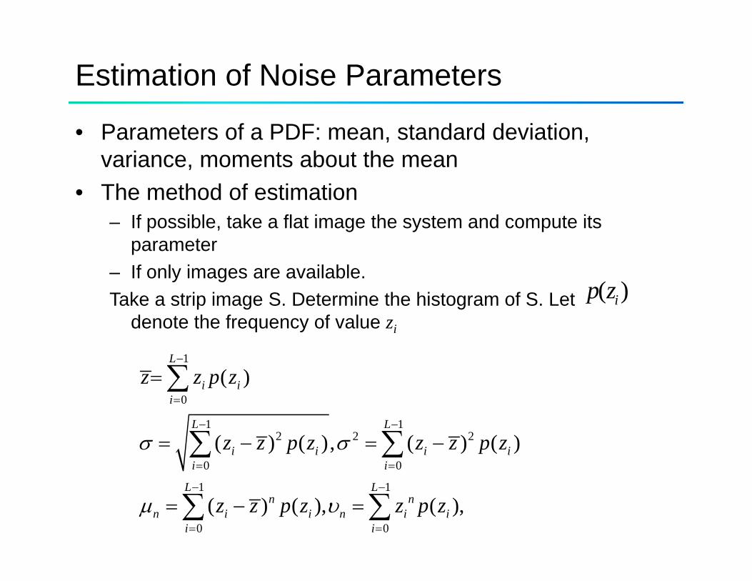
• Parameters of a PDF: mean, standard deviation, variance, moments about the mean

• The method of estimation– If possible, take a flat image the system and compute its

parameterp– If only images are available. Take a strip image S. Determine the histogram of S. Let

denote the frequency of value zi

( )ip zdenote the frequency of value zi

1

0( )

L

i ii

z z p z−

=

= ∑0

1 12 2 2

0 0

( ) ( ), ( ) ( )

i

L L

i i i ii i

z z p z z z p zσ σ

=

− −

= =

= − = −∑ ∑1 1

0 0

( ) ( ), ( ),L L

n nn i i n i i

i i

z z p z z p zμ υ− −

= =

= − =∑ ∑

Spatial filters based restoration technique

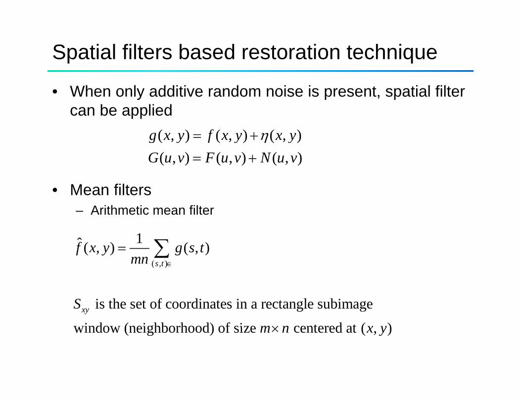
• When only additive random noise is present, spatial filter can be applied

( , ) ( , ) ( , )( , ) ( , ) ( , )

g x y f x y x yG u v F u v N u v

η= += +

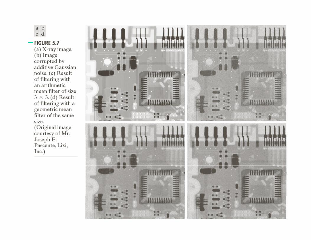
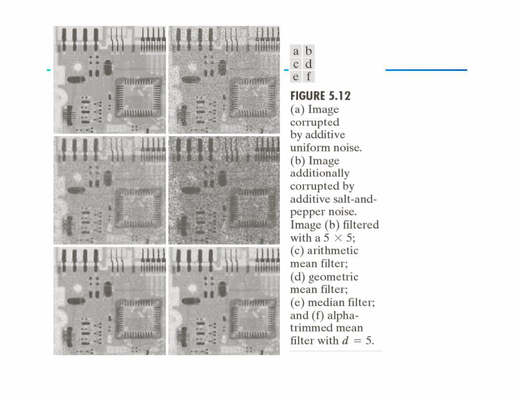
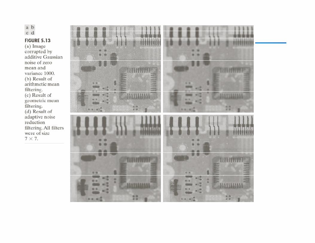
• Mean filters – Arithmetic mean filter

( , )

1ˆ ( , ) ( , )s t

f x y g s tmn ∈

= ∑

is the set of coordinates in a rectangle subimage

window (neighborhood) of size centered at ( )xyS

m n x y×window (neighborhood) of size centered at ( , )m n x y×

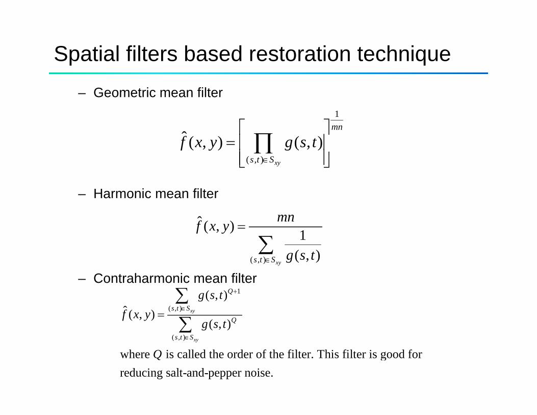
Spatial filters based restoration technique – Geometric mean filter

1mn⎡ ⎤

( , )

ˆ ( , ) ( , )xy

mn

s t S

f x y g s t∈

⎡ ⎤= ⎢ ⎥⎢ ⎥⎣ ⎦∏

– Harmonic mean filter

ˆ ( , ) 1mnf x y =

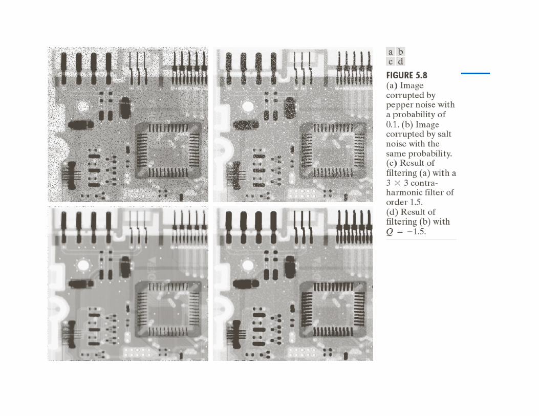
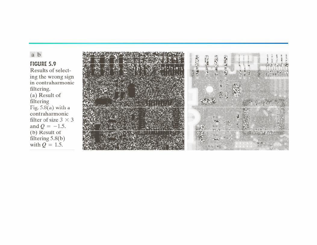
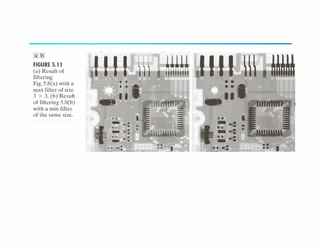
– Contraharmonic mean filter( , )

1( , )

xys t S g s t∈∑

1

( , )

( )

( , )ˆ ( , )

( , )xy

Q

s t S

Q

s t S

g s tf x y

g s t

+

∈

∈

=∑

∑( , )

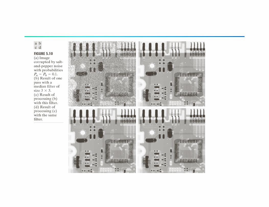
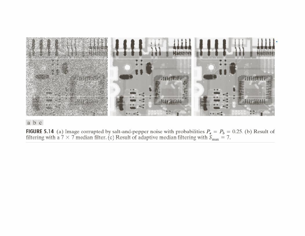
where is called the order of the filter. This filter is good for reducing salt-and-pepper noise.

xys t S

Q∈