approaches to parameter and variance estimation in
TRANSCRIPT

Approaches to parameter and variance estimation ingeneralized linear models
Eugenio Andraca Carrera
A dissertation submitted to the faculty of the University of North Carolina at ChapelHill in partial fulfillment of the requirements for the degree of Doctor of Philosophy inthe Department of Biostatistics.
Chapel Hill2008
Approved by:
Bahjat Qaqish, Advisor
Lisa LaVange, Reader
Lloyd Edwards, Reader
John Preisser, Reader
Ibrahim Salama, Reader
Victor Schoenbach, Reader
Abstract
EUGENIO ANDRACA CARRERA: Approaches to parameter and varianceestimation in generalized linear models.(Under the direction of Bahjat Qaqish.)
In many studies of clustered binary data, it is reasonable to consider models in which
both response probability and cluster size are related to unobserved random effects. Two
resampling methods have been recently proposed in the literature for mean parameter
estimation in this setting: within-cluster resampling (WCR) and within-cluster paired
resampling (WCPR). These procedures are believed to provide valid estimates in the
presence of nonignorable cluster size. We identify the parameters estimated under WCR
and under unweighted generalized estimating equations and elaborate on their differences
and validity. We propose a simple weighted generalized estimating equations strategy
that is asymptotically equivalent to WCPR but avoids the intensive computation in-
volved in WCPR. We investigate the parameter estimated by WCPR for a generalized
mixed model. We show that the parameter estimated by WCPR may be affected by
factors other than the actual effects of exposure and propose an alternative strategy for
the analysis of correlated binary data with cluster-specific intercepts based on simple
generalized estimating equations for random intercept-matched pairs.
We study the problem of variance estimation in small samples using robust or sand-
wich variance estimators. Robust variance estimators are widely used in linear regression
with heteroscedastic errors, generalized linear models with possibly misspecified variance
model, and generalized estimating equations. In these settings, the robust variance es-
timator provides asymptotically consistent estimates of the covariance matrix of mean
parameters. However, the robust variance estimator may severely underestimate the
ii

true variance in studies with small sample size. Bias-corrected versions of the robust
variance estimator have been proposed to improve its small sample performance. We
introduce a new class of corrected robust variance estimators with an emphasis on vari-
ance reduction and small sample performance. These estimators are applicable to linear
regression, generalized linear models and generalized estimating equations. We show in
simulations that the new estimators perform better in terms of variance and confidence
interval coverage than many current estimators, while maintaining comparable average
confidence interval width.
iii

Acknowledgments
I am deeply grateful to my advisor, Dr. Bahjat Qaqish, for his guidance and support in
my doctoral research. He has been an outstanding mentor throughout this process. He
always patiently answered my questions and provided insightful discussions. I would also
like to express my gratitude to the members of my dissertation committee: Dr. Lloyd
Edwards, Dr. Lisa LaVange, Dr. John Preisser, Dr. Ibrahim Salama and Dr. Victor
Schoenbach. Thank you for your support and useful suggestions and comments. Thank
you also to the wonderful people of the department of Biostatistics at UNC. It has been
a real pleasure to be a part of this department for the past six years.
I would especially like to thank my family: Mom, Dad, Alejandro and Martha, and
my wonderful fiancee Lisa. Thank you for your love and your prayers. I couldn’t have
done it without you.
Finally, I would like to thank the financial support of the Consejo Nacional de Ciencia
y Tecnologıa, CONACYT, and the Amgen dissertation fellowship. Your generous help
has allowed me to complete my graduate studies and write this dissertation.
iv
Table of Contents
List of Figures viii
List of Tables ix
List of Abbreviations x
1 Introduction and literature review 1
1.1 Introduction . . . . . . . . . . . . . . . . . . . . . . . . . . . . . . . . . . 1
1.1.1 Cluster resampling methods . . . . . . . . . . . . . . . . . . . . . 1
1.1.2 Variance estimation . . . . . . . . . . . . . . . . . . . . . . . . . . 2
1.2 Literature review: within cluster resampling . . . . . . . . . . . . . . . . 3
1.2.1 Random effects models . . . . . . . . . . . . . . . . . . . . . . . . 3
1.2.2 Within cluster resampling . . . . . . . . . . . . . . . . . . . . . . 4
1.3 Literature review: within-cluster paired resampling . . . . . . . . . . . . 6
1.4 Literature review: variance estimation . . . . . . . . . . . . . . . . . . . 7
1.4.1 Notation . . . . . . . . . . . . . . . . . . . . . . . . . . . . . . . . 8
1.4.2 Review of estimators . . . . . . . . . . . . . . . . . . . . . . . . . 9
1.4.3 Bias, variance and performance . . . . . . . . . . . . . . . . . . . 13
1.4.4 Correlated data . . . . . . . . . . . . . . . . . . . . . . . . . . . . 17
1.4.5 Summary . . . . . . . . . . . . . . . . . . . . . . . . . . . . . . . 21
v

2 Random cluster size, within-cluster resampling and generalized esti-mating equations 22
2.1 Introduction . . . . . . . . . . . . . . . . . . . . . . . . . . . . . . . . . . 22
2.2 Within-cluster unit resampling . . . . . . . . . . . . . . . . . . . . . . . . 23
2.3 A beta-binomial model and associated parameters . . . . . . . . . . . . . 25
2.3.1 The model . . . . . . . . . . . . . . . . . . . . . . . . . . . . . . . 25
2.3.2 Estimation by WCR . . . . . . . . . . . . . . . . . . . . . . . . . 26
2.3.3 Estimation by GEE . . . . . . . . . . . . . . . . . . . . . . . . . . 27
2.3.4 Examples of nonignorable cluster size . . . . . . . . . . . . . . . . 28
2.4 Within cluster paired resampling . . . . . . . . . . . . . . . . . . . . . . 30
2.5 A mixed model and associated parameters . . . . . . . . . . . . . . . . . 33
2.5.1 The model . . . . . . . . . . . . . . . . . . . . . . . . . . . . . . . 33
2.5.2 An alternative GEE estimator . . . . . . . . . . . . . . . . . . . . 34
2.5.3 Example . . . . . . . . . . . . . . . . . . . . . . . . . . . . . . . . 35
2.6 Discussion . . . . . . . . . . . . . . . . . . . . . . . . . . . . . . . . . . . 36
3 Variance estimation in regression models 38
3.1 Introduction . . . . . . . . . . . . . . . . . . . . . . . . . . . . . . . . . . 38
3.2 Heteroscedasticity-consistent covariance estimators . . . . . . . . . . . . 40
3.2.1 A class of variance estimators . . . . . . . . . . . . . . . . . . . . 40
3.2.2 Generalized linear models (GLM) . . . . . . . . . . . . . . . . . . 42
3.2.3 Properties . . . . . . . . . . . . . . . . . . . . . . . . . . . . . . . 43
3.3 Simulations . . . . . . . . . . . . . . . . . . . . . . . . . . . . . . . . . . 45
3.4 Examples . . . . . . . . . . . . . . . . . . . . . . . . . . . . . . . . . . . 50
3.5 Discussion . . . . . . . . . . . . . . . . . . . . . . . . . . . . . . . . . . . 54
vi

4 Variance estimation for correlated data 63
4.1 Introduction . . . . . . . . . . . . . . . . . . . . . . . . . . . . . . . . . . 63
4.1.1 Notation . . . . . . . . . . . . . . . . . . . . . . . . . . . . . . . . 64
4.2 Independent Data . . . . . . . . . . . . . . . . . . . . . . . . . . . . . . . 65
4.3 Correlated Data . . . . . . . . . . . . . . . . . . . . . . . . . . . . . . . . 67
4.3.1 A class of variance estimators for correlated data . . . . . . . . . 69
4.3.2 Computational issues . . . . . . . . . . . . . . . . . . . . . . . . . 71
4.4 Simulations . . . . . . . . . . . . . . . . . . . . . . . . . . . . . . . . . . 73
4.5 Example . . . . . . . . . . . . . . . . . . . . . . . . . . . . . . . . . . . . 78
4.6 Discussion . . . . . . . . . . . . . . . . . . . . . . . . . . . . . . . . . . . 80
5 Summary and future research 87
5.1 Summary of accomplishments . . . . . . . . . . . . . . . . . . . . . . . . 87
5.1.1 Chapter 2: Random cluster size, within-cluster resampling andgeneralized estimating equations . . . . . . . . . . . . . . . . . . . 87
5.1.2 Chapter 3: Variance estimation in regression models . . . . . . . . 88
5.1.3 Chapter 4: Variance estimation for correlated data . . . . . . . . 88
5.2 Future research . . . . . . . . . . . . . . . . . . . . . . . . . . . . . . . . 89
5.2.1 Robust variance estimation in other settings . . . . . . . . . . . . 89
5.2.2 Other topics . . . . . . . . . . . . . . . . . . . . . . . . . . . . . . 91
Appendix 93
References 99
vii

List of Figures
2.1 True βWCPR by cluster size and exposure probability . . . . . . . . . . . 37
3.1 Per capita income and per capita spending in public schools . . . . . . . 62
viii

List of Tables
2.1 Parameters estimated by WCPR and expected proportion ofXY -informativeclusters . . . . . . . . . . . . . . . . . . . . . . . . . . . . . . . . . . . . . 37
2.2 Analysis of dental data . . . . . . . . . . . . . . . . . . . . . . . . . . . . 37
3.1 Coverage of estimators OLS, HC3, HC3(1), HC4 and HC4(1) . . . . . . . 56
3.2 Bias of estimators OLS, HC3, HC3(1), HC4 and HC4(1) . . . . . . . . . . 57
3.3 Confidence intervals fitting a logistic model for binomial data to beta-binomial data . . . . . . . . . . . . . . . . . . . . . . . . . . . . . . . . . 58
3.4 Confidence intervals fitting a Poisson model to gamma-Poisson data . . . 59
3.5 Analysis of overdispersed binary data . . . . . . . . . . . . . . . . . . . . 60
3.6 Beta-binomial simulations based on Crowder’s data . . . . . . . . . . . . 61
3.7 Analysis of Greene’s data . . . . . . . . . . . . . . . . . . . . . . . . . . . 61
4.1 Multivariate normal data with common cluster size ni = 4. Varianceestimation of cluster-level parameter. . . . . . . . . . . . . . . . . . . . 83
4.2 Multivariate normal data with common cluster size ni = 4. Varianceestimation of subject-level parameter . . . . . . . . . . . . . . . . . . . . 84
4.3 Variance estimation for correlated binary data . . . . . . . . . . . . . . . 85
4.4 Analysis of progabide data . . . . . . . . . . . . . . . . . . . . . . . . . . 86
ix

List of Abbreviations
CWGEE Cluster weighted generalized estimating equations
GEE Generalized estimating equations
GLM Generalized linear models
HCCME Heteroscedasticity-consistent covariance estimators
OLS Ordinary least squares
MINQUE Minimum norm quadratic estimator
WCPR Within-cluster resampling
WCR Within-cluster paired resampling
x

Chapter 1
Introduction and literature review
1.1 Introduction
1.1.1 Cluster resampling methods
Studies involving correlated or clustered binary data arise often in medical applications.
Statistical tools have been proposed to analyze clustered binary data for various study
designs and parametrizations. Random-effect models and marginal models are commonly
used by researchers depending on whether interest lies in subject-specific effects or pop-
ulation average effects. Within-cluster resampling (WCR) was suggested by Hoffman,
Sen and Weinberg (2001) as a procedure for parameter estimation in marginal models
where response probability and cluster size are related to unobserved random effects.
A similar method, within-cluster paired resampling (WCPR), was suggested by Rieger
and Weinberg (2002) for estimation of subject-specific effects in models resembling a
matched-pairs setup. They proposed WCPR for the analysis of correlated binary data
with cluster-specific intercepts and slopes.
Even though WCR and WCPR have gained popularity in the literature, it is not clear
what parameters they estimate and how they differ from generalized estimating equations
(GEE). Hoffman et al. (2001) claim that unweighted generalized estimating equations
is not a valid estimating procedure when cluster size is related to response probability.

Similarly, Rieger and Weinberg (2003) suggest that conditional logistic regression (CLR)
is not a valid estimating procedure in the presence of cluster-specific intercepts and
slopes. WCR and WCPR are proposed as alternative estimating approaches in these
settings. In §1.2 and §1.3 we review the available literature on WCR and WCPR. In
Chapter 2 we investigate the parameters estimated by WCR, WCPR and unweighted
generalized estimating equations in various models. We show that WCR and WCPR can
be written in terms of specially weighted estimating equations. We study the parameters
induced by WCR, WCPR and GEE and comment on the validity of each procedure.
1.1.2 Variance estimation
WCR and WCPR are methods of mean parameter estimation for correlated data. Statis-
tical inference of these mean parameters requires estimates of their variance. The robust
or ‘sandwich’ variance estimator, introduced by Liang and Zeger (1986), is widely used
to estimate the covariance matrix of mean parameters in correlated data. One of the
main advantages of the robust variance estimator is that it provides consistent estimates
of the true covariance matrix of the parameters of interest, even if the variance model
is misspecified. It is applicable in settings such as linear regression with heteroscedas-
tic errors and generalized linear models. However, it has been shown that the robust
variance estimator may lead to anti-conservative inference in small samples in many sit-
uations. Corrections to the robust variance estimator have been proposed to improve its
small sample performance. Most corrections to the sandwich estimator available in the
literature focus on reducing its bias. Kauermann and Carroll (2001) showed that the
robust variance estimator has higher variance than parametric variance estimators when
the parametric model is correct. They showed that the increased variance of the robust
variance estimator results in a loss of efficiency.
In §1.4 we review the literature on robust variance estimation; we cover variance
estimators for linear regression with heteroscedastic errors, as well as their bias, variance
2

and performance. In section 1.4.4 we review variance estimation for correlated data. In
Chapter 3 we introduce a new family of variance estimators for linear regression and
generalized estimating equations that includes some of the estimators introduced in §1.4
as well as new estimators not previuosly considered in the literature. We show that some
of the new estimators have smaller variance than currently available estimators and that
this translates into improved confidence interval coverage. In Chapter 4 we extend the
family of variance estimators to correlated data. We show that new estimators improve
upon current estimators in terms of variance and coverage in simulations with correlated
Gaussian data and correlated binary data. In Chapter 5 we summarize the results of the
previous chapters and discuss future research.
1.2 Literature review: within cluster resampling
1.2.1 Random effects models
One common approach to account for within-cluster correlation in correlated data is
through random effects models. We introduce one such model with a random intercept
for binary data.
Consider a study with K clusters, indexed by i = 1, . . . , K and observations within
cluster i indexed by j = 1, . . . , ni. Let the jth binary response in the ith cluster be
denoted by Yij, and let it be related to a (p× 1) vector of covariates xij through
logit(E(Yij)) = αi + x>ijβ. (1.1)
If αi in model (1.1) can be assumed to follow a probability distribution dependent on
parameters θ under some regularity conditions, then a random effects model eliminates αi
by estimating θ and the fixed slope β through likelihood methods. Models with logit link
and cluster-specific random effects were first proposed by Cox (1958) and Rasch (1961).
Laird (1982) proposed the use of random effects models for the analysis of longitudinal
3

data and Stiratelli et al. (1984) extended random effects models to correlated binary
data. The interpretation of β may be marginal if random effects are integrated out or
conditional within a cluster.
Neuhaus et al. (1992) showed that misspecification of the random effects distribution
may lead to bias in regression coefficients, however this bias tends to be small. Neuhaus
and McCulloch (2006) then showed that ignoring the correlation between covariates and
random effects may also lead to biased regression coefficients.
An alternative to random effects models, marginal methods for the analysis of cor-
related binary data based on generalized estimating equations became available after
the work of Liang and Zeger (1986) and Zeger and Liang (1986). The GEE approach
assumes mean and variance models for the response and accounts for within-cluster as-
sociation by using a working correlation matrix for each cluster’s vector of responses Yi.
We discuss generalized estimating equations in more detail later in this document in the
context of sandwich variance estimators for correlated data.
1.2.2 Within cluster resampling
Hoffman et al. (2001) proposed WCR for the analysis of correlated binary data with
nonignorable cluster size. They define nonignorable cluster size as any violation of the
property E(Yij|ni, Xij) = E(Yij|Xij). In particular, they consider a model where re-
sponse probability and cluster size are related to an unobserved random effect. Hoffman
et al. (2001) claim that unweighted generalized estimating equations is not a valid
method of estimation when cluster sizes are nonignorable and propose WCR as a valid
estimation alternative.
The WCR procedure is based on sampling one observation from each cluster at each
of Q resampling steps. The q-th data set then consists of one independent observation
from each cluster. A regression model for independent data is fit to the q-th resample
and an estimate of mean parameters and their covariance matrix is obtained. The WCR
4

estimate is obtained by pooling the estimators obtained at each resampling step. The
WCR procedure is described in detail in Chapter 2.
Williamson, Datta and Satten (2003) and Benhin, Rao and Scott (2005) showed that
the WCR procedure is equivalent to generalized estimating equations with independence
working correlation structure and cluster weight equal to the inverse of cluster size.
Neuhaus and McCulloch (2006) discussed Hoffman et al.’s (2001) paper and suggested
that nonignorable cluster size be considered as a misspecification of the random effects
distribution. They argue that the bias of slope coefficients in the simulations of Hoffman
et al. (2001) and Williamson et al. (2003) is small, and that only the intercept shows
significant bias. Neuhaus and McCulloch (2006) claim that these results are consistent
with their research on misspecified random effects distribution (Neuhaus et al., 1992).
Even though the simulations of Hoffman et al. (2001) and Williamson et al. (2003)
show small bias in slope coefficients and small differences between estimates obtained
by unweighted GEE and WCR, their data examples show large differences between
estimates obtained by the two approaches. In Chapter 2 we explain the differences
between unweighted GEE and WCR in these simulations and data examples.
Follmann, Proschan and Leiffer (2003) extended the use of within cluster resampling
to applications including angular data, p-values and Bayesian inference. Cong, Yin
and Shen (2007) and Williamson et al. (2008) used WCR to model correlated survival
data where the outcome of interest is associated with cluster size. Datta and Satten
(2005; 2007) extended WCR to rank-tests and signed-ranked tests in situations with
‘informative cluster sizes’. Our work focuses on the application of WCR to correlated
binary data.
Recent areas of application of WCR include cross-sectional surveys in epidemiology
(Williamson, Kim and Warner, 2007), veterinary epidemiology (Faes et al., 2006) and
genetic association in families (Shin et al., 2007). Faes et al. (2006) note that an
alternative approach to WCR, with a different parameter interpretation, is to include
5

cluster size as a covariate in the model. While this model may be useful in many
scenarios, we do not explore it further.
1.3 Literature review: within-cluster paired resam-
pling
Rieger and Weinberg (2003) proposed within cluster paired resampling for the analysis of
correlated binary data for models with cluster-specific intercepts and slopes. The method
is based on resampling two observations from each cluster such that one observation
has response yij = 1 while the other has response yik = 0. Clusters with at least one
y-discordant pair are called ‘informative clusters’. The resulting resampled data set
resembles data from a matched-pair design. Conditional logistic regression based on the
resampled pairs is then used to estimate the parameter vector β. The final estimate
βWCPR is the mean of Q resamples.
Conditional logistic regression has been widely used in case-control studies (Breslow
and Day, 1980). CLR assumes a cluster-specific intercept or random effect. Through
conditioning, CLR eliminates random intercepts and estimates conditional or cluster-
specific slope parameters. CLR makes no distributional assumptions about the random
effects. It assumes independent outcomes within clusters conditional on the random ef-
fects and a conditional slope parameter β common to all clusters. These two assumptions
are not required if all clusters have only two observations each and the data resemble
a matched-pair design. This is the motivation of the WCPR method: the resampling
procedure proposed by Rieger and Weinberg (2002) produces resampled data sets con-
taining one pair of y-discordant observations from each informative cluster and resembles
a matched-pair design. The WCPR is studied in more detail in Chapter 2.
Rieger, Kaplan and Weinberg (2001) proposed a less general version of WCPR based
on sampling one affected and one unaffected sibling from each sibship in family studies
6

to test for linkage and association between a disease and candidate genes. The authors
named their method ‘Within Sibship Paired Resampling’ (WSPR). Both WCPR and
WSPR have met limited discussion in the literature. Our research aims to improve the
understanding of WCPR and offer alternative analysis tools for estimation of cluster
level parameters for correlated binary data. The results on WCPR are easily extended
to the special case of WSPR for use in family-based case-control studies.
1.4 Literature review: variance estimation
Consider the linear model E(Y) = Xβ,Var(Y) = Γ where Y is an n × 1 vector of
responses, X is a known n × p matrix of covariates of rank p, β is a p × 1 vector of
unknown parameters, and Γ = diag(γ1, . . . , γn) is unknown.
The ordinary least squares estimator of β, given by β = (XTX)−1XTY, is best
linear unbiased under homoscedasticity, γ1 = · · · = γn = σ2. It also remains unbiased
under heteroscedasticity, but is no longer best unbiased. Asymptotically, for large n, β
is consistent under fairly general conditions (Eicker, 1963). The ordinary least squares
estimator (OLS) of cov(β),
(XTX)−1
n∑i=1
r2i /(n− p),
where ri = Yi − xTi β, is based on the assumption of homoscedasticity. This estimator is
the one typically printed out by most regression software. In general, the true covariance
is given by
cov(β) = (XTX)−1XTΓX(XTX)−1. (1.2)
The OLS variance estimator is generally biased under heteroscedasticity and can lead
to gross undercoverage of corresponding confidence intervals. This weakness of the OLS
7

estimator has long been recognized and several alternative estimators exist.
The goal of this section is to review some of the most relevant approaches to es-
timate (1.2) under heteroscedasticity in the literature. It is organized as follows. In
§1.4.1 we introduce some notation. In §1.4.2 we review variance estimators proposed
for linear models with heteroscedasticity. In §1.4.3 we study issues of bias, variance and
performance of some of these variance estimators in published simulation studies. §1.4.4
reviews variance estimators available for correlated data.
1.4.1 Notation
We will use the following notation throughout this dissertation. If a = (a1, · · · , an)T is
a vector, then diag(a) will denote a diagonal matrix with diagonal elements a1, · · · , an.
Conversely, if A is a square matrix with elements aij, then diag(A) will denote the
column vector (a11, · · · , ann)T .
For any two vectors or matrices B = (bij) and C = (cij) of the same dimensions,
we denote their Schur product (Marcus and Minc, 1964, p.120) as B ∗C := (bijcij).
Consequently, the k-th Schur power of B is denoted by B∗k = (bkij).
The ‘hat matrix’ H = (hij) is given by H = X(XTX)−1XT . Its diagonal elements,
hii, are called ‘leverages’. Also, let the vector of squared residuals be denoted by S, with
elements r2i . Finally, let us define the matrix P := (I − H)∗2 where I is the identity
matrix.
Estimators of the true covariance are generally obtained by replacing Γ in (1.2) by
an estimator Γ = diag(γ). Since Γ is diagonal, we may write it in full matrix form Γ
or, equivalently, in vector form γ. When talking about individual components of Γ we
write γi, where it is understood that γi = Γii.
8
1.4.2 Review of estimators
Early work on estimators of cov(β) and their properties can be traced to Eicker (1963)
and Huber (1967). Eicker anticipated the results of White (1980) by studying conditions
for the asymptotic normality of (β−β)/cov(β) where cov(β) is obtained by replacing Γ
by cov(rirTi ) in (1.2). Huber (1967) further studied the asymptotic properties of cov(β)
under maximum likelihood methodology.
Hartley et al. (1969) and Rao (1970) proposed the first variance estimators unbiased
under heteroscedasticity for a wide range of linear models. Rao (1970) named this class
of estimators MINQUE (minimum norm quadratic estimator). Estimators derived from
MINQUE such as the almost unbiased estimator soon followed (Horn et al., 1975). In
1980, White proposed a heteroscedasticity-consistent covariance matrix estimator. His
estimator, denoted HC0, is often used by researchers in fields such as economics and
social sciences, and is commonly available in most software packages (Long and Ervin,
2000). Since White’s (1980) seminal paper, modified White estimators such as HC1,
HC2 and HC3 have appeared in the literature. The performance of these estimators in
small samples has been studied extensively by MacKinnon and White (1985), Long and
Ervin (2000), Flachaire (2005), and many more.
In the following sections we introduce some of these estimators as well as some others
related to our work. Later, we discuss some of the literature available regarding their
performance in small samples, as well as issues of bias and variance.
MINQUE
Hartley et al. (1969) proposed unbiased estimators for a linear model with a stratified
design with one unit per stratum and unequal variances. Their estimator can be written
as γ = P−1S. The estimator of Hartley et al. (1969) is included in a larger class of
estimators referred to as MINQUE by Rao (1970).
Consider a linear combination αTγ =∑αiγi to be estimated. A quadratic form
9

YTAY is said to be MINQUE of αTγ if A = (aij) is such that ‖A‖ is minimized
subject to
AX = 0 and∑
aiiγi ≡∑
αiγi.
These two conditions guarantee invariance to translation of β and unbiasedness of
YTAY as an estimator of αTγ.
MINQUE exist for more general linear models than the model of interest of this
review. The model we consider is that of independent, unreplicated data with variances
that are unknown and possibly all different. For this model the unreplicated MINQUE
corresponds to the estimator of Hartley et al. (1969) (Horn et al. 1975).
Even though MINQUE are unbiased, they exhibit some undesirable properties. First,
existence of MINQUE is not guaranteed; it is conditional on P being non-singular. Rao
(1970) gives sufficient conditions for the existence of P−1, however these conditions are
not simple. Second, even if MINQUE exist, it is possible to obtain negative estimators
of some γi and Var(zT β) for some p × 1 vector z in finite samples (Horn et al., 1975;
Dorfman, 1991). Finally, MINQUE seems to exhibit large variance in many scenarios
(Chesher and Jewitt, 1987; Bera, Suprayitno and Premaratne, 2002).
HC0. White’s estimator
White’s 1980 paper on a heteroscedasticity-consistent covariance matrix estimator is
one of the most influential papers in the field. His HC0 estimator is simply obtained by
replacing Γ in (1.2) by Γ(0)
:= diag(S).
Since the expected value of the vector of squared residuals is given by E(S) = Pγ it
follows that White’s estimator is biased for finite samples. The extent of HC0’s bias was
studied by Chesher and Jewitt (1987). Issues of bias and performance are considered in
the following section.
10

White’s (1980) major contribution was showing that
(XTX)−1XT Γ(0)
X(XTX)−1 p−→ (XTX)−1XTΓX(XTX)−1
under either homoscedasticity or heteroscedasticity under regularity conditions. It allows
researchers to conduct adequate inference under unknown heteroscedasticity for large
enough samples.
HC1, HC2 and HC3
Several finite sample corrections to White’s estimator have been proposed in the litera-
ture. Perhaps the simplest one was given by Hinkley (1977). Hinkley’s estimator HC1
is a degrees of freedom corrected version of HC0 given by
HC1 :=n
n− pHC0.
In 1975, Horn et al. proposed the almost unbiased estimator, also known as HC2.
The HC2 estimator of Γ can be written componentwise as γ(1)i = r2
i /(1 − hii) and in
vector form as γ(1) = DS. The HC2 estimator of cov(β) is obtained by replacing
Γ(1)
= diag(γ(1)) in (1.2). Horn et al. (1975) proposed HC2 based on the fact that the
expected value of the squared residuals E(S) = Pγ depends on both Γ and the leverages
hii through P. This estimator is unbiased under homoscedasticity, but in general it is
biased under heteroscedasticity.
The HC3 estimator closely approximates the jackknife estimator of Miller (1974).
The HC3 is obtained by replacing Γ(2)
in (1.2), where γ(2) = D2S. It be written com-
ponentwise as γ(2)i = r2
i /(1− hii)2. The HC3 estimator is biased upwards.
It is known that HC0, HC1, HC2 and HC3 are consistent for cov(β) under some
regularity conditions. Dorfman (1991) proved that estimators obtained by replacing Γ(δ)
in (1.2) where γ(δ)i = r2
i /(1 − hii)δ are consistent for any fixed δ ≥ 0 as long as the
11
leverages are bounded so that max1≤i≤n(hii) → 0 as n → ∞. HC0, HC2 and HC3 are
special cases with δ = 0, 1 and 2.
Other estimators
Other estimators have been proposed in the literature. We discuss two of them by
Cribari-Neto et al. (2000) and Cribari-Neto (2004).
Cribari-Neto et al. (2000) proposed a sequence of modified White estimators of Γ
with decreasing bias that is related to both HC0 and MINQUE. They argued that the
k-th estimator in the sequence has bias of order O(n−(k+2)). Their sequence of estimators
γ(0), . . . , γ(k) is defined in the following way:
1. Let γ(0) = S, White’s estimator.
2. Let Bγ(k)(γ) := E(γ(k))− γ.
3. Obtain the k-th estimator in the sequence by subtracting the estimated bias from
the (k − 1)-th estimator evaluated at γ(0) , that is γ(k) = γ(k−1) −Bγ(k−1)(γ(0)).
Cribari-Neto et al. (2000) showed that after k iterations
γ(k) =k∑j=0
(−1)jM (j)(γ(0))
where M (j) = (P− I)jγ(0). Using this notation, their k-th estimator can be written as
γ(k) =
(k∑j=0
(I−P)j
)S.
As k → ∞, γ(k) converges to P−1S, the unreplicated MINQUE, if P−1 exists and
diverges otherwise. This result follows from a generalization of the geometric series
commonly known as the von Neumann series. This result was not explicitly noted by
Cribari-Neto et al. (2000)
12

This sequence of estimators has some undesirable properties. First, if P is not in-
vertible, then the sequence γ(k) is divergent. Second, even if P−1 exists, γ(k) may have
some negative elements γi(k) < 0 for some i ∈ {1, . . . , n} for any k ≥ 1.
Another estimator proposed recently in the literature is the HC4 estimator of Cribari-
Neto (2004). Elementwise HC4 is defined by γi = r2i /(1− hii)δi where
δi = min
(4,
nhii∑nj=1 hii
).
The idea behind HC4 is to inflate the i-th residual by a larger factor than HC3 when
hii is large relative to h =∑n
j=1 hii/n. Cribari-Neto (2004) found that HC4 performed
better than HC3 and HC0 in terms of test size relative to nominal size in simulations.
The HC4 estimator is a potentially useful alternative to HC3 when the design matrix X
includes points of very high leverage. However, HC4 tends to be more biased than HC3
and usually leads to wider confidence intervals.
In the following sections we review results on bias, variance and performance in
confidence intervals of the estimators introduced in this section. We find that most
authors recommend the use of HC3 over competing estimators.
1.4.3 Bias, variance and performance
In many applications, interest lies in estimation and inference on the linear combi-
nation zT β for some p × 1 vector z. Let aT = zT (XTX)−1XT and let us define
υ := Var(zT β) = aTΓa. The estimators discussed so far differ in terms of bias and
variance of corresponding υ = aT Γa. These differences affect the way estimators υ be-
have in terms of confidence interval coverage relative to nominal size, power and width
of confidence intervals.
In this section we review the work of Chesher and Jewitt (1987) on limits on the
bias of HC0, HC2 and the jackknife estimator, and the work of Kauermann and Carroll
13
(2001) on the role of variance on the efficiency of covariance matrix estimators. Finally,
we discuss the performance of these estimators in simulations under heteroscedasticity.
Bias
Chesher and Jewitt (1987) studied the role of heteroscedasticity and design on the bias
of HC0, HC2 and the jackknife estimator. They found bounds on the bias of these
estimators in terms of the true Γ and the leverages hii. We present some of their results.
Let α = maxi(γi)/mini(γi) be a measure of the level of heteroscedasticity present
in the model. Chesher and Jewitt (1987) show that if heteroscedasticity is moderate,
α < 2, then the HC0 estimator υ(0) = aT Γ(0)
a is biased downward for any p × 1 vector
z. However, if α > 2, it is possible for White’s estimator to be biased upward.
Let pb(υ(0)) :=(E(υ(0))− υ
)/υ be the proportionate bias of υ(0). Under homoscedas-
ticity Chesher and Jewitt (1987) show that
−max(hii) ≤ pb(υ(0)) ≤ −min(hii).
Under heteroscedasticity, they derive the following results
pb(υ(0)) ≤ max(αhii(1− hii) + hii(hii − 2))
and
−max(hii)(1/α− 1) ≤ pb(υ(1)) ≤ −max(hii)(α + 1)
where υ(1) corresponds to the HC2 estimator. A similar result is derived for the jackknife
estimator and therefore to a close approximation for HC3.
The importance of these results is twofold. First, they allow us to set bounds on
the bias of HC0, HC1, HC2 and HC3 under known moderate heteroscedasticity in terms
of Γ and under unknown heteroscedasticity in terms of the design. Second, Chesher
and Jewitt (1987) show that the bias of HC0-HC3 is not dependent only on the level
14
of heteroscedasticity, but that it can be strongly affected by the design, specially in the
presence of high leverage points.
Variance
Kauermann and Carroll (2001) studied the variance of the robust or sandwich variance
estimator in the linear model and in quasi-likelihood models and generalized estimating
equations. They showed that the sandwich estimator has higher variability than para-
metric variance estimators when the parametric model is correct and that the extent of
the extra variance depends on the design. Increased variance of the variance estimators
translates into confidence intervals with subnominal coverage.
Let p = 1− α be the quantile of the normal distribution for a given α. Kauermann
and Carroll (2001) show that variance relates to coverage through the following theorem,
we quote:
Theorem 2. Let θ ∼ N(θ, σ2/n) and let σ2 be an unbiased estimator of σ2
independent of θ. The coverage probability of the 1 − α confidence interval
CI(σ2, α) equals
Pr{θ ∈ CI(σ2, α)} = 1− α− cpVar(σ2)
σ4+O(n−2)
where cp = φ(zp)(z3p + zp)/8, with φ(·) the standard normal distribution
density.
The authors then suggest a coverage adjustment to construct confidence intervals
based on normal quantiles. This adjustment is based on homoscedastic errors. They
show in simulations that their correction reduces undercoverage of sandwich estimators
in the heteroscedastic case but may still result is subnominal coverage, particularly in
the presence of points of high leverage.
15

Kauermann and Carroll (2001) state that: “...undercoverage is determined mainly
by the variance of the variance estimator”. Their work suggests that variance reduction
of variance estimators is highly important when constructing confidence intervals of
regression parameters in small samples.
Further work has focused on the issues of bias and variance of heteroscedasticity
consistent variance estimators. Motivated by the work of Chesher and Jewitt (1987),
Bera et al. (2002) studied the variance of MINQUE. They found that MINQUE may have
very large variance particularly for highly unbalanced design matrices. Qian and Wang
(2001) studied the influence of high leverage points on the bias of White’s (1980) and
Hinkley’s (1977) estimators. They proposed bias-corrected versions of these estimators
with a focus on reducing variance and MSE of υ. Our work focuses on a class of variance
estimators with reduced variance.
Performance
There has been considerable research on the performance of HC0-HC3 estimators in
terms of confidence interval coverage under heteroscedasticity. We comment on three
influential papers on the problem by MacKinnon and White (1985), Long and Ervin
(2000) and Cribari-Neto (2004).
MacKinnon and White (1985) compared HC1, HC2 and the jackknife estimator under
different scenarios of heteroscedasticity in simulations with sample sizes 50, 100 and 200.
The jackknife is closely approximated by the HC3 estimator (Dorfman, 1991; Long and
Ervin, 2000); therefore conclusions regarding the jackknife should apply to HC3. Long
and Ervin (2000) compared HC0-HC3 in simulations with sample sizes as small as 25.
The conclusions of both articles are as follows:
• The OLS may lead to severely misleading inference under heteroscedasticity.
• Tests of heteroscedasticity lack power in small samples. When heteroscedasticity
is suspect, the OLS should be replaced by HC3.
16

• HC3 performs better than HC0-HC2 in studies with sample size less than 250; for
larger sample sizes the choice of variance estimator does not matter as much.
• White’s estimator (HC0) underestimates the variance in small samples and leads
to undercoverage of confidence intervals. The HC0 estimator should not be used
in small samples, even though this seems to be common practice in research and
software (Long and Ervin, 2000).
Cribari-Neto (2004) followed a different approach and studied the influence of high
leverage points on confidence interval coverage of HC0, HC3 and HC4 estimators. He
found that HC3 may perform poorly in the presence of points of high leverage and that
HC4 is more robust to influential observations. The disadvantage of HC4 in relation to
HC3 comes in the form of wider average confidence intervals and larger variance.
1.4.4 Correlated data
Correlated data are common in medical studies where each cluster contributes multiple
observations to a study. The theory on the use of the robust variance estimator for
correlated data can be traced back to the work of Huber (1967), Hartley et al. (1969)
and White (1980), as discussed in previous sections. Liang and Zeger (1986) and Zeger
and Liang (1986) extended the use of the robust variance estimator to generalized es-
timating equations. Since then, the robust variance estimator has gained popularity in
the literature and is routinely used by researchers in many disciplines. We introduce
some basic results on generalized estimating equations and robust variance estimation
for correlated data.
Consider a clustered study with M total clusters. Let ni denote the size of the i-th
cluster and let observations within it be denoted by yij, j = 1, . . . , ni. The response of
interest yij is related to a p × 1 vector of covariates xij through g(µij) = xTijβ where
µij = E(yij|xij). Let µi = {µi1, . . . , µini}T and let the vector of all responses be written as
17
Y = {YT1 , . . . ,Y
TM}T . Also let cov(Yi) = Γi and the block-diagonal matrix cov(Y) = Γ.
The generalized estimating equations methodology of Liang and Zeger (1986) estimate
β by solving the equations
Uβ,GEE1 =M∑i=1
DiV−1i (Yi − µi) = 0
where Di := ∂µi/∂βT , Vi := diag(σ
12ijj)Ri(α)diag(σ
12ijj), Ri is a working correlation
matrix for corr(yi) and σijj = µij(1− µij).
Estimators of cov(β) are obtained by replacing estimators of Γi in
(M∑i=1
DTi V−1
i Di
)−1( M∑i=1
DTi V−1
i ΓiV−1i Di
)(M∑i=1
DTi V−1
i Di
)−1
. (1.3)
The robust variance estimator of Liang and Zeger (1986), denoted here by BC0,
is obtained by replacing Γi by Γi := rirTi in (1.3) where ri = (yi − µi). Liang and
Zeger (1986) showed that the robust variance estimator provides consistent estimates of
regression parameters in correlated data even when the covariance of the responses is
misspecified. However it has been shown that the robust variance estimator is usually
biased downwards in small samples and leads to Wald tests that are too liberal (Mancl
and DeRouen, 2001; Fray and Graubard, 2001; Lipsitz et al., 1994). This topic is
discussed in more detail in Chapter 4.
Several approaches have been suggested to improve estimation of cov(β) and the
performance of Wald tests in small samples. Two corrections to the sandwich variance
estimator given by Kauermann and Carroll (2001) and Mancl and DeRouen (2001) are
especially relevant to our work.
Kauermann and Carroll (2001) suggest using
Γi := (Ini −Hii)−1/2rir
Ti (Ini −Hii)
−1/2T
18

in (1.3) where Hij = Di
(∑Kl=1 DT
l V−1l Dl
)−1
DTj V−1
j . This estimator will be referred
to as BC1. The matrix Hii is the leverage of the i-th subject (Preisser and Qaqish,
1996) and can be seen as a generalization of the univariate hii. The rationale behind
Kauermann and Carroll’s (2001) correction is that if E((yi−µi)(yi−µi)T ) = σ2Vi then
E(zTBC1z) = Var(zT β){1 +O(K−2)} for any p× 1 vector z.
Mancl and DeRouen (2001) suggested the correction
Γi := (Ini −Hii)−1rir
Ti (Ini −Hii)
−1T
in (1.3). Mancl and DeRouen’s (2001) estimator will be referred to as BC2. Their
derivation follows a different argument than Kauermann and Carroll (2001). They obtain
the first order approximation
E(rirTi ) ≈ (Ii −Hii)Γi(Ii −Hii)
T +∑j 6=i
HijΓjHTij
and drop the summation in the expression above assuming its contribution is negligible.
Both corrected estimators improve upon the standard sandwich estimator in terms of
confidence interval coverage. Lu et al. (2007) compared both estimators in a simulation
study. They found that in general BC2 provides coverage closer to nominal than BC1
except in studies with small cluster sizes, where BC2 may lead to overcoverage. An
interesting note is that the observed bias of BC2 is expected to be larger than the bias
of BC1 in most situations even though BC2 provides coverage closer to nominal. An
explanation for this behavior is that positive bias in variance estimators may compensate
for their variability when constructing confidence intervals (Lu et al., 2007). Kauermann
and Carroll (2001) results on the variance of the variance estimator discussed in the
previous section extend to generalized estimating equations. They show that the variance
of the sandwich estimator directly affects the coverage of confidence intervals. The
research of Lu et al. (2007) and Kauermann and Carroll (2001) strongly suggests that
19

both bias and variance of sandwich variance estimators should be taken into account
when constructing confidence intervals of regression parameters with either independent
or correlated data. In Chapter 4 we study variance estimation for correlated data in
more detail. We introduce a class of variance estimators that includes BC0, BC1 and
BC2 as well as some new estimators. We compare estimators in this class in simulation
scenarios for correlated data. We show that newly proposed estimators perform better
in terms of variance and confidence interval coverage than BC0, BC1 and BC2.
The literature includes other approaches to constructing sandwich variance estimators
and corresponding Wald tests for studies with correlated data. We briefly name some
of them. Fay and Graubard (2001) proposed a modification to the sandwich estimator
based on the first order Taylor expansion of the expectation of the i-th squared residual.
They also suggested evaluating corresponding Wald tests as an F ratio with degrees of
freedom that are a function of the estimated variance of the sandwich estimator. Pan
and Wall (2002) also suggested a correction to the degrees of freedom of t or F tests
as a function of the variance of the variance estimator. Approaches based on degrees of
freedom corrections have met limited success (Lu et al., 2007; Braun, 2007). McCaffrey
and Bell (2006) introduced a bias-reduction correction to the sandwich estimator in the
setting of correlated binary data along with a Satterthwaite correction to the degrees of
freedom of corresponding t tests. However, their method may not work adequately in
the presence of high intra-cluster correlation. Morel et al. (2003) suggest a correction
to the sandwich estimator based on adding a fraction of the naive variance estimator.
Braun (2007) studied the problem from the point of view of cluster randomized trials.
He suggested combining GEE regression estimates with variance estimators based on
penalized quasi-likelihood and corrected Wald tests. The methods of Morel (2003) and
Braun (2007) seem to work adequately in terms of coverage of confidence intervals in
many situations; however the correction of Mancl and DeRouen (2001) seems to perform
better with a small number of clusters (Braun, 2007). Some of the approaches above are
20

not exclusive: Pan and Wall (2003) and Braun (2007) discuss the possibility of using
corrected estimators such as Mancl and DeRouen’s (2001) together with a Wald test
correction. Our work focuses on corrections to the sandwich variance estimator rather
than degrees of freedom corrections of Wald tests. However, both are viable areas of
research.
1.4.5 Summary
We introduced two methods for mean parameter estimation for correlated binary data:
within cluster resampling and within-cluster paired resampling. WCR was proposed for
marginal parameter estimation in situations where cluster size may be related to response
probability. WCPR was proposed for conditional parameter estimation for models with
cluster-specific intercepts and slopes. The literature on WCR and WCPR does not iden-
tify the parameters estimated by each approach clearly. A comparison of the parameters
estimated by WCR, WCPR and unweighted GEE is needed to gain understanding of
these procedures. Our work aims to compare these estimation approaches, clarify their
differences and comment on their validity.
We reviewed the topics of robust variance estimation for linear models under het-
eroscedasticity and correlated data. The robust variance estimator is asymptotically
consistent but usually anti-conservative in small samples. Several corrections improve
the small sample performance of the robust variance estimator. Most corrections fo-
cus on the bias of the variance estimator. Kauermann and Carroll (2001) showed that
the variance of the variance estimator is largely responsible for interval undercoverage
in small samples. The goal of our work is to propose a new class of robust variance
estimators with an emphasis on variances reduction and small sample performance.
21

Chapter 2
Random cluster size, within-cluster
resampling and generalized
estimating equations
2.1 Introduction
Correlated binary data are common in public health and biomedical applications. Several
statistical tools have been developed to analyze this type of data, such as random-effect
models (Laird and Ware, 1982) and generalized estimating equations (GEE) (Liang and
Zeger, 1986). An interesting problem arises when both response and cluster size are as-
sociated with unobserved random effects. Hoffman, Sen and Weinberg (2001) proposed
‘within cluster resampling’ (WCR) for the analysis of correlated binary data with nonig-
norable cluster size, defined as any violation of the property E(Yij|ni, Xij) = E(Yij|Xij).
They use nonignorable cluster size in the context of a random effects model in which clus-
ter size Ni is random and associated with an unobserved random effect Pi. Their method
is based on resampling units within clusters. Williamson, Datta and Satten (2003) and
Benhin, Rao and Scott (2005) showed that resampling in WCR can be avoided through
the use of cluster-weighted generalized estimating equations. Rieger and Weinberg (2003)

proposed within cluster resampling of pairs of discordant observations for estimation of
conditional parameters.
In this chapter we investigate the parameters estimated by unit-resampling, pair-
resampling and generalized estimating equations. We explore the validity of unit-resampling
and generalized estimating equations in studies with non-ignorable cluster sizes and pro-
pose a new method of estimation for conditional parameters with correlated binary data.
Our analysis extends the understanding of these models and the strengths and weak-
nesses of these estimation procedures.
This chapter is organized as follows. In §2.2 we describe the WCR procedure. In
§2.3 we introduce the model used by Hoffman et al. (2001) and Williamson et al. (2003)
and investigate the parameters estimated by WCR and GEE in their model and two
other models. In §2.4 we describe within cluster paired resampling (WCPR). In §2.5 we
introduce the model used by Rieger and Weinberg (2003), study the parameter estimated
by WCPR and propose an alternative estimating method. §2.6 is a conclusion.
2.2 Within-cluster unit resampling
Consider a study with K clusters, indexed by i = 1, . . . , K. Let observations within
cluster i be indexed by j = 1, . . . , ni. Let the jth binary response in the ith cluster be
denoted by Yij with corresponding p×1 vector of covariates xij. Throughout this section
we consider the logistic model
logitE(Yij; xij) = x>ijβ (2.1)
where β is a parameter vector to be estimated.
The WCR procedure can be summarized as follows: a data set is obtained by ran-
domly selecting one observation from each cluster. Thus each resample consists of K
independent observations. Then by fitting a regression model for independent data to
23

the q-th resample, an estimate β(q), and an estimate of its covariance matrix Σ(q), are
obtained. The resampling procedure is repeated Q times. The final estimate is the mean
of the Q estimates,
βWCR =1
Q
Q∑q=1
β(q), (2.2)
and its covariance is estimated by
Σ =1
Q
Q∑q=1
Σ(q)− Sβ, (2.3)
where Sβ is the sample covariance matrix of the Q estimates.
We analyze the WCR procedure to identify what parameters it estimates. The q-th
resample is identified by the sampling vector
Z(q) = (Z1(q), · · · , ZK(q))>,
where the components of Z(q) are independent and Zi(q) is an integer drawn randomly
from the set {1, · · · , ni}. The estimate β(q) is the solution in β of the estimating
equation
Uq(β; Z(q)) :=K∑i=1
ni∑j=1
I(Zi(q) = j)xij(yij − µij) = 0,
where µij := E[Yij]. We use Ec to denote expectations with respect to resampling,
conditioned on the data. The expected value of Uq(β; Z(q)) conditional on the data is
Ec[Uq(β;Z(q))] =K∑i=1
1
ni
ni∑j=1
xij(yij − µij). (2.4)
Thus when both K and Q are large, and under standard regularity conditions, βWCR
24
is equivalent to the solution of
UWCR(β) :=K∑i=1
1
ni
ni∑j=1
xij(yij − µij) = 0. (2.5)
The above estimating equation is a weighted generalized estimating equations with
independence working correlation structure and cluster weight 1/ni. This equivalence is
useful for two purposes. First, the computational burden of the resampling procedure can
be avoided and the same estimate obtained by using generalized estimating equations
with independence working correlation structure and cluster weight 1/ni. This can
be easily implemented in standard software for generalized estimating equations. The
covariance matrix can be estimated by the sandwich variance estimator. This has been
shown by Williamson et al. (2003).
Second, the parameter estimated by WCR can be found as the solution of E[UWCR(β)] = 0
where the expectation is taken under the model of interest.
2.3 A beta-binomial model and associated parame-
ters
2.3.1 The model
The WCR procedure of Hoffman et al. (2001) was not derived in the context of a specific
model. However, the model gleaned from their simulations is a mixed model of the beta-
binomial type in which cluster size is random and is correlated with the cluster-specific
random effect. Here we describe the model used in the simulation section of Williamson
et al. (2003) which differs only in some minor numerical details from that of Hoffman
et al. (2001). There is a single cluster-level binary covariate xi. The random effect Pi is
distributed as beta(a0, b0) if xi = 0 and beta(a1, b1) if xi = 1. The parameters (al, bl) are
chosen such that for xi = 0 the mean of Pi, a0/(a0 + b0) = 0.25 and the within-cluster
25

correlation 1/(a0 + b0 + 1) = 0.15. For xi = 1 the mean of Pi is 0.35 and the within-
cluster correlation is 0.25. This gives a0 = 17/12, b0 = 4.25, a1 = 1.05 and b1 = 1.95.
Conditional on Pi, cluster size Ni follows a truncated binomial(9, g(Pi)) where values
0, 1, 8 and 9 are discarded. The binomial probability g(Pi) is as follows: g(Pi) = 0.25
if Pi > E[Pi] and g(Pi) = 0.75 if Pi ≤ E[Pi]. Conditional on Pi and Ni, the response
Ti :=∑ni
j=1 Yij follows a binomial(Ni, Pi) distribution.
2.3.2 Estimation by WCR
We now investigate the parameters estimated by WCR. Let β = (β0, β1)> and πi(β) be
the function
πi(β) := {1 + exp(−β0 − β1xi)}−1.
In the context of the above model, (2.5) can be written as
UWCR(β) =K∑i=1
1
Ni
(1, xi)T{Ti −Niπi(β)} =
K∑i=1
(1, xi)T{ TiNi
− πi(β)}.
We assume that Pr(Ni > 0) = 1. This implies that βWCR is the limit solution in β
of
K∑i=1
(1, xi)T
{E
[TiNi
]− πi(β)
}= 0. (2.6)
Under the model of section (2.3.1), E[Ti|Ni, Pi] = NiPi which implies that
E
[TiNi
|Ni, Pi
]= Pi, (2.7)
and by unconditioning
E
[TiNi
]= E[Pi].
Thus if E[Pi] follows a logistic regression on xi with parameters β∗, then β∗ will be
26

the limit solution of (2.6), that is βWCR = β∗. That is certainly the case in the model
given above, and the parameters are
β∗0 = logit(0.25) ≈ −1.099, β∗1 = logit(0.35)− logit(0.25) ≈ 0.48.
Note that in the above derivation the critical condition is (2.7); as long as
E[TiNi
|Ni, Pi] = Pi,
WCR estimates the same parameter regardless of the dependence, or lack thereof, be-
tween Ni and Pi.
On a technical note, we have assumed uniqueness of the limiting root of (2.6) which,
strictly speaking, follows from other considerations. The required conditions are not
restrictive and we assume that they hold. A similar assumption is made below.
2.3.3 Estimation by GEE
The estimating function for unweighted generalized estimating equations is
UGEE(β) =K∑i=1
(1, xi)T {Ti −Niπi(β)}.
Its expected value with respect to both Yi and Ni is
E[UGEE(β)] =K∑i=1
(1, xi)T {E[Ti]− πi(β)E[Ni]}.
So βGEE, the parameter estimated by unweighted generalized estimating equations
is the limit solution in β of
K∑i=1
E[Ni] (1, xi)T
{E[Ti]
E[Ni]− πi(β)
}= 0.
27

For the model given above,
E[Ni;xi = 0] = 4.72, E[Ti;xi = 0] = 0.957,
E[Ni;xi = 1] = 4.66, E[Ti;xi = 1] = 1.31,
with corresponding βGEE = (−1.37, 0.43)>. The mean parameter estimates reported by
Williamson et al. (2003) from their simulation study, (−1.382, 0.429)> for K = 50 and
(−1.366, 0.418)> for K = 500, are in close agreement with the theory.
Essentially, unweighted generalized estimating equations are valid for fitting the
model
logitE[Ti]
E[Ni]= β0 + β1xi, (2.8)
while weighted generalized estimating equations with cluster weight 1/Ni and, equiva-
lently, WCR are valid for fitting the model
logit E[TiNi
] = β0 + β1xi. (2.9)
Both methods are valid for their respective models, and the choice of estimation
method should be based on whether the model of interest is (2.8) or (2.9). The two
models coincide only if, for all i, E[Ti]/E[Ni] = E[Ti/Ni], a condition equivalent to
Cov(Ti/Ni, Ni) = 0.
2.3.4 Examples of nonignorable cluster size
The purpose of these examples is to show that the choice of estimation procedure should
be based on examination of the model and its parameters.
28

A missing data model
Let Yij , j = 1, . . . , n∗i , be i.i.d. Bernoulli variables with mean pi given by
logit pi = β0 + β1xi,
where xi is a cluster level binary covariate. Let {Zij, j = 1, · · · , n∗i } be missingness
indicators such that Zij = 1 if Yij is observed and Zij = 0 if Yij is missing, and suppose
that
γs := Pr(Zij = 1|Yij = s), s = 0, 1,
with γ0 6= γ1.
Suppose we observe only Ti =∑n∗i
j=1 YijZij and Ni =∑n∗i
j=1 Zij. Nonignorability of
cluster size can be seen by comparing E[Yij] = pi to E[Yij|Ni = n∗i ] = piγ1/{piγ1 + (1−
pi)γ0}. Unweighted GEE fit the model (2.8) given by
logitE[Ti]
E[Ni]= logit
piγ1
piγ1 + (1− pi)γ0
= β∗0 + β1xi, (2.10)
where β∗0 = β0 + log(γ1/γ0). If the data are limited to clusters with Ni > 0 then (2.9)
becomes
logitE[TiNi
|Ni > 0] = logitE[Ti|Ni > 0]
E[Ni|Ni > 0]= β∗0 + β1xi
and both WCR and GEE fit (2.10). The proof is in the appendix. This example shows
that it is possible for WCR and GEE to estimate the same parameters in the presence
of nonignorable cluster sizes.
A model for developmental toxicity
Kuk (2003) developed a model for fetal response in developmental toxicity in which
both the number of fetal implants as well as the death or malformation of implanted
fetuses are dose dependent. The model produces ignorable cluster sizes according to the
29

definition of Hoffman et al. (2001), but Kuk (2003) argues that failure to consider the
association between dose and fetal implantation might underestimate the total effect of
exposure.
Let N0 be the unobserved cluster size that would have been observed in the absence
of a toxic agent. Through the concept of thinning, the observed cluster size is assumed
to have mean exp(α1xi)E(N0) where xi represents dose level of a toxic agent and α1 ≤ 0.
Given that a fetus is implanted, the probability of death or malformation pi is inde-
pendent of cluster size and is modeled by
logitpi = β0 + β1xi.
Under this model E[Ti/Ni] = E[Ti]/E[Ni] = pi and the parameters estimated under
WCR and GEE will both asymptotically converge to β0 and β1.
Kuk (2003) argues that pi itself is not the measure of risk of interest for developing
a virtually safe dose, since it ignores the negative effect of the toxic agent on fetal
implantation. He proposes a combined risk that takes into account the probability of
failure to implant and the probability of successful implantation leading to malformation
or death. This is the risk measure of interest in the model. In this case cluster size is
associated with exposure in a way that leads to ignorable cluster size according to the
definition by Hoffman et al. (2001). While WCR and GEE provide consistent estimates
of β0 and β1, both underestimate the total risk associated with exposure.
2.4 Within cluster paired resampling
Rieger and Weinberg (2003) proposed within cluster paired resampling (WCPR) for
the analysis of correlated binary data for models with cluster-specific intercepts and
slopes. The method is based on resampling two observations from each cluster such
that one observation has response yij = 1 and the other has response yik = 0. This
30
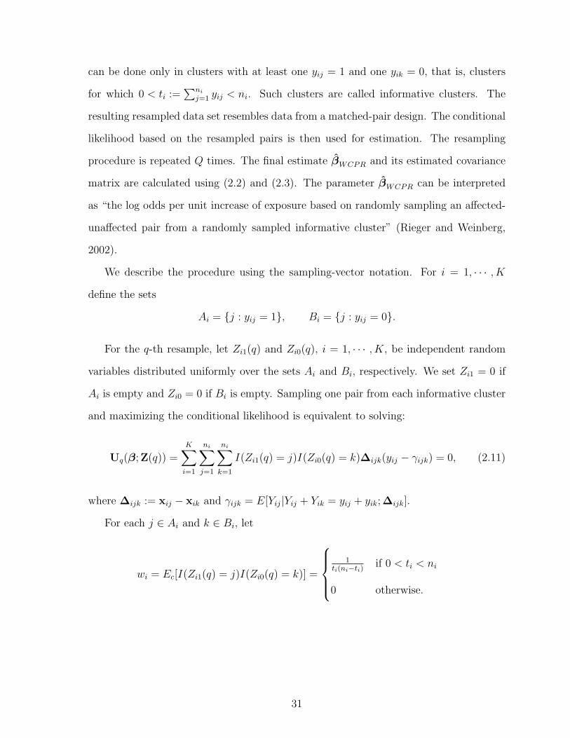
can be done only in clusters with at least one yij = 1 and one yik = 0, that is, clusters
for which 0 < ti :=∑ni
j=1 yij < ni. Such clusters are called informative clusters. The
resulting resampled data set resembles data from a matched-pair design. The conditional
likelihood based on the resampled pairs is then used for estimation. The resampling
procedure is repeated Q times. The final estimate βWCPR and its estimated covariance
matrix are calculated using (2.2) and (2.3). The parameter βWCPR can be interpreted
as “the log odds per unit increase of exposure based on randomly sampling an affected-
unaffected pair from a randomly sampled informative cluster” (Rieger and Weinberg,
2002).
We describe the procedure using the sampling-vector notation. For i = 1, · · · , K
define the sets
Ai = {j : yij = 1}, Bi = {j : yij = 0}.
For the q-th resample, let Zi1(q) and Zi0(q), i = 1, · · · , K, be independent random
variables distributed uniformly over the sets Ai and Bi, respectively. We set Zi1 = 0 if
Ai is empty and Zi0 = 0 if Bi is empty. Sampling one pair from each informative cluster
and maximizing the conditional likelihood is equivalent to solving:
Uq(β; Z(q)) =K∑i=1
ni∑j=1
ni∑k=1
I(Zi1(q) = j)I(Zi0(q) = k)∆ijk(yij − γijk) = 0, (2.11)
where ∆ijk := xij − xik and γijk = E[Yij|Yij + Yik = yij + yik; ∆ijk].
For each j ∈ Ai and k ∈ Bi, let
wi = Ec[I(Zi1(q) = j)I(Zi0(q) = k)] =
1
ti(ni−ti) if 0 < ti < ni
0 otherwise.
31

Then the expected value of Uq(β; Z(q)) conditional on the data is
Ec[Uq(β; Z(q))] =K∑i=1
wi∑
j∈Ai,k∈Bi
∆ijk(yij − γijk). (2.12)
Empty sums are taken to be zero.
We propose solving UWCPR := Ec[Uq(β; Z(q))] = 0 to estimate β. We will refer
to this strategy as ‘cluster weighted generalized estimating equation’ (CWGEE). This
can be implemented in standard software by converting each informative cluster to a
pseudo-cluster consisting of ti(ni − ti) observations with responses yij = 1, yik = 0,
associated covariate vectors ∆ijk and cluster weight wi. A standard logistic regression
model with no intercept is fitted using yij as response, and with an independence working
correlation structure. For large K and Q, the weighted CWGEE estimator is equivalent
to the WCPR estimator. This follows from arguments similar to those of Williamson et
al. (2003).
The CWGEE approach offers advantages over WCPR. First, CWGEE avoids the
intensive computation involved in WCPR. Second, in a resampled data set in WCPR,
some elements of ∆ijk can be 0 for most or every sampled pair, resulting in infinite
or undefined parameter estimates. This may happen in studies with small number of
clusters or where the exposure of interest is rare. The instability of the resampling-
based estimates, especially with small K, has been noted by Hoffman et al. (2001) and
Williamson et al. (2003). In contrast, CWGEE does not suffer from this problem unless
it is a global issue affecting the whole data set.
32

2.5 A mixed model and associated parameters
2.5.1 The model
In this section we investigate the nature of the parameter estimated by WCPR, to be
denoted βWCPR, in a generalized mixed model used in Rieger and Weinberg (2002). We
consider K clusters of equal size and a single binary covariate Xij that may vary within
a cluster. Covariates Xij’s are mutually independent. Several values of the prevalence
of exposure, Pr(Xij = 1), will be investigated.
The intercept parameter is fixed at α = logit(0.25). The cluster-specifc random slope
βi takes two possible values with probability 1/2 each. Given this structure, βWCPR is
the root of the expected value of (2.12), that is, the solution of
K∑i=1
∑yi,xi, bi
Pr(Yi = yi,Xi = xi, βi = bi) · wi∑
j∈Ai,k∈Bi
∆ijk(Yij − γijk) = 0, (2.13)
where Pr(Yi,Xi, βi) is computed under the model as Pr(Yi,Xi, βi) = Pr(Xi = xi) ·
Pr(βi = bi) · Pr(Yi = yi|xi, bi).
We calculate βWCPR for each simulation setup of Rieger and Weinberg (2002).
Table 2.1 summarizes the results for the case ni = 4 and Pr(Xij = 1) = 0.5. It
can be seen that, in general, βWCPR 6= E[βi]. The table also shows the probability that
a random cluster contributes an XY -informative pair, a pair that is discordant with
respect to both Y and X. This is important because in the resampling scheme, only
XY -informative pairs contribute to the conditional likelihood. The table shows that,
for the setups considered, only about 34-42% of the clusters are expected to provide
informative pairs. This implies that the resample estimates will be highly unstable when
K is small, and thus a very large Q may be needed.
The parameter βWCPR is a function not only of the distribution of βi, but also of the
intercept parameter, cluster size and exposure prevalence. This property is illustrated
33

in Figure 2.1. In this setup the intercept and the distribution of βi are held fixed. The
plot shows that cluster size and exposure probability have a large impact on the value
of βWCPR. The impact of exposure prevalence is especially large for large cluster sizes.
For example, when the common cluster size is 3 and the probability of exposure is 0.1,
βWCPR = 0.1650, which may suggest that exposure is a risk factor. When the common
cluster size is 8 and the probability of exposure is 0.9, βWCPR = −0.2270, which may now
suggest that the exposure has a protective effect. The attractiveness of WCPR is that it
is simple to describe. However, this comes at the high cost of βWCPR being affected by
factors other than the actual effects of exposure. When applying or using WCPR, this
feature must be kept in mind.
2.5.2 An alternative GEE estimator
Alternative estimating methods for the analysis of correlated binary data for models
with cluster-specific intercepts and slopes can be obtained by applying different weights
than CWGEE in (2.12). We propose solving
UUWGEE :=K∑i=1
∑j∈Ai,k∈Bi
∆ijk(yij − γijk) = 0. (2.14)
We will refer to this approach as UWGEE. The parameter βWCPR obtained by either
WCPR or CWGEE can be interpreted as “the log odds per unit increase of exposure
based on randomly sampling an affected-unaffected pair from a randomly sampled infor-
mative cluster” (Rieger and Weinberg, 2002). The parameter βUWGEE that solves (2.14)
is interpreted as “the log odds per unit increase of exposure based on randomly sampling
an affected-unaffected matched pair from the population of all such matched pairs”.
The advantage of βUWGEE over βWCPR is that βUWGEE is not affected by cluster size
and exposure prevalence. For example, the value of βUWGEE is 0.165 for all combinations
of cluster size and exposure probability shown in Figure 2.1.
34

2.5.3 Example
We analyzed data from the Intergenerational Epidemiologic Study of Adult Periodontitis
known as Multi-Pied (Gansky et. al, 1998; 1999). The study included 467 subjects. The
number of teeth per person ranged between 2 and 32 with a mean of 21. For each person
in the study the investigators recorded the mean clinical attachment level, in mm, by
type of tooth. The binary outcome of interest is whether the mean clinical attachment
exceeded 3 mm. We consider one binary covariate: whether a tooth is categorized as
posterior (molar or premolar) or anterior (cuspid or incisor) and fit the logistic model
logitE(Yij|αi, β,MOLARij) = αi + β(MOLARij), (2.15)
where MOLARij is an indicator of whether the jth tooth in the ith subject is posterior.
This is the same model used by Rieger and Weinberg (2003) but with a different data set.
The parameter of interest β is interpreted as the log odds of mean clinical attachment
exceeding 3 mm of a molar tooth compared to an anterior tooth based on randomly
sampling a pair of affected-unaffected teeth from a randomly sampled person with at
least one such pair of teeth.
We fit the model using WCPR with 1000, 5000 and 10000 resamples and with the
CWGEE and UWGEE approaches. Our analysis used only the 167 subjects with at least
one affected-unaffected pair of teeth. Table 2.2 shows estimates of β and corresponding
standard errors. Results under CWGEE and WCPR with a large number of resamples
were very similar. Under CWGEE we obtained β = 0.1064 with estimated standard
error 0.1339. Under WCPR with 10,000 resamples we obtained β = 0.1070 (0.1354).
The close agreement between the two methods was expected due to the asymptotic
equivalence of the WCPR and the CWGEE estimators. The UWGEE method obtains
β = 0.0925 (0.1449).
35

2.6 Discussion
We investigated two within-cluster resampling procedures. The difference between unit
resampling and unweighted generalized estimating equations is that they estimate dif-
ferent models and have different target parameters. With that in mind, both WCR and
unweighted generalized estimating equations are robust to dependence between Ni and
Pi. The choice of procedure should be based on whether the model of interest is (2.8)
or (2.9).
For the paired resampling procedure, the computational cost can be avoided by using
a special version of weighted generalized estimating equations that is easily implemented
in standard software. The attractiveness of WCPR is that it is simple to describe and
implement. However, its target parameter is unduely sensitive to cluster size and ex-
posure prevalence. An alternative version of generalized estimating equations with unit
weights estimates a target parameter that is not affected by cluster size distribution and
exposure prevalence. Since cluster size and, more importantly, exposure distribution are
not intrinsically related to exposure risk, the alternative procedure is preferable.
36

Table 2.1: Parameters estimated by WCPR and expected proportion of XY -informativeclusters
βi values E(βi) βWCPR % XY-informative0.3/-0.3 0 0.01990 34.21.5/-0.3 0.6 0.67050 40.02.0/-0.3 0.85 0.89470 42.41.2/-1.2 0 0.26340 36.32.0/-2.0 0 0.54799 39.2
0.992/-2.5 -0.754 -0.03677 33.91.026/-2.9 -0.937 -0.04004 33.90.934/-1.8 -0.433 -0.00017 34.21.046/-2.5 -0.727 -0.00223 34.2
βi values assigned with probability 1/2, clustersize = 4, α = logit(0.25), exposure prevalence = 0.5 .
Table 2.2: Analysis of dental data
β (SE)UWGEE 0.0925 (0.1449)CWGEE 0.1064 (0.1339)WCPR
1,000 resamples 0.0986 (0.1360)5,000 resamples 0.1109 (0.1392)10,000 resamples 0.1070 (0.1354)
37

Figure 2.1: True βWCPR by cluster size and exposure probability
Clusters assigned βi = −2.5 or βi = 1.25 with probability 1/2.Common intercept α = logit(0.25).
38

Chapter 3
Variance estimation in regression
models
3.1 Introduction
Consider again the linear model introduced in Chapter 1: EY = Xβ,Var(Y) = Γ where
Y is an n× 1 vector of responses, X is a known n× p matrix of covariates of rank p, β
is a p× 1 vector of unknown parameters, and Γ = diag(γ1, . . . , γn) is unknown.
In Chapter 1 we stated that the ordinary least squares (OLS) estimator of β is best
linear unbiased only under homoscedasticity and that the OLS estimator of cov(β) is
biased and leads to improper inference under heteroscedasticity. We introduced variance
estimators that are robust to heteroscedasticity. The goal of this chapter is to introduce
a class of robust variance estimators for independent data that includes some currently
available estimators as well as some new estimators. We evaluate estimators in this class
in terms of confidence interval coverage under homoscedasticity and some scenarios of
heteroscedasticity.

Throughout this chapter, we use the notation introduced in 1.4.1. If a = (a1, · · · , an)T
is a vector, we write diag(a) to denote a diagonal matrix with diagonal elements a1, · · · , an.
Conversely, if A is a square matrix with elements aij, then diag(A) will denote the col-
umn vector (a11, · · · , ann)T . H denotes the hat matrix H = X(XTX)−1XT , and S is the
vector of squared residuals with elements r2i , where ri = Yi − xTi β.
Heteroscedasticity-consistent covariance estimators (HCCME) of the true covariance,
cov(β) = (XTX)−1XTΓX(XTX)−1, (3.1)
are generally obtained by replacing Γ in (3.1) by an estimator. The most commonly
used HCCME, the ‘sandwich’, ‘empirical’ or ‘robust’ variance estimator, was proposed
by White in 1980. White’s estimator, γi = r2i , is biased in finite samples (Chesher and
Jewitt, 1987) and can lead to inadequate coverage of confidence intervals. Several correc-
tions to White’s estimator have been proposed to reduce its bias or improve its coverage.
A well known class of HCCMEs is given by γi = r2i /(1− hii)δ (Dorfman, 1991), where
hii are the diagonal elements of H and δ ≥ 0. White’s estimator is obtained with δ = 0,
the ‘almost unbiased’ estimators of Horn et al. (1975) and Wu (1986) with δ = 1 and the
jackknife estimator of Miller (1974) with δ = 2 to a close approximation. These three
estimators are referred to as HC0, HC2 and HC3 respectively (Long and Ervin, 2000).
Cribari-Neto (2004) proposed HC4, given by γi = r2i /(1− hii)δi with δi = max(4, hii/h),
for designs with high leverage points. Estimators HC0-HC3 have been evaluated by
MacKinnon and White (1985) and Flachaire (2005), among others.
The HC2 estimator is unbiased only under homoscedasticity. The HC3 and HC4
40

are generally biased upwards. However, bias is not the only concern with the sandwich
estimator. In fact, bias can be removed completely; since E[S] = Pγ, where P has
elements that are the squares of the corresponding elements of (I −H), the estimator
γ = P−1S is exactly unbiased for γ = diag(Γ). Horn et al. (1975) show that this
estimator is the (unreplicated) MINQUE (minimum norm quadratic estimator) with
uncorrelated and heteroscedastic errors of Rao (1970). Even though the MINQUE is
unbiased, it has large variance (Bera et al., 2002) and can have negative components.
Kauermann and Carroll (2001) identified high variability of the sandwich estimator as a
source of poor coverage of confidence intervals. We show that reducing the variance of
covariance estimators results in improved coverage of confidence intervals. This chapter
is organized as follows. In §3.2 we describe the new class of estimators; in §3.3 we present
simulation studies; in §3.4 we show data analysis examples; §3.5 is a conclusion.
3.2 Heteroscedasticity-consistent covariance estima-
tors
3.2.1 A class of variance estimators
We consider estimators of the true covariance of cov(β) obtained by replacing Γ in (3.1)
by an estimator. Since Γ is a diagonal matrix, we limit our attention to the vector of its
diagonal elements γ = diag(Γ). We define the class of estimators of γ:
γ(k)δ = Dδ−1(DP)kDS, (3.2)
41
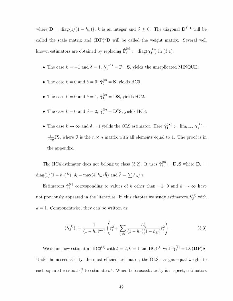
where D = diag{1/(1 − hii)}, k is an integer and δ ≥ 0. The diagonal Dδ−1 will be
called the scale matrix and (DP)kD will be called the weight matrix. Several well
known estimators are obtained by replacing Γ(k)
δ := diag(γ(k)δ ) in (3.1):
• The case k = −1 and δ = 1, γ(−1)1 = P−1S, yields the unreplicated MINQUE.
• The case k = 0 and δ = 0, γ(0)0 = S, yields HC0.
• The case k = 0 and δ = 1, γ(0)1 = DS, yields HC2.
• The case k = 0 and δ = 2, γ(0)2 = D2S, yields HC3.
• The case k →∞ and δ = 1 yields the OLS estimator. Here γ(∞)1 := limk→∞γ
(k)1 =
1n−pJS, where J is the n × n matrix with all elements equal to 1. The proof is in
the appendix.
The HC4 estimator does not belong to class (3.2). It uses γ(0)δ∗
= D∗S where D∗ =
diag(1/(1− hii)δi), δi = max(4, hii/h) and h =∑hii/n.
Estimators γ(k)δ corresponding to values of k other than −1, 0 and k → ∞ have
not previously appeared in the literature. In this chapter we study estimators γ(1)δ with
k = 1. Componentwise, they can be written as:
(γ(1)δ )i =
1
(1− hii)δ−1
(r2i +
∑j 6=i
h2ij
(1− hii)(1− hjj)r2j
). (3.3)
We define new estimators HC3(1) with δ = 2, k = 1 and HC4(1) with γ(1)δ∗
= D∗(DP)S.
Under homoscedasticity, the most efficient estimator, the OLS, assigns equal weight to
each squared residual r2i to estimate σ2. When heteroscedasticity is suspect, estimators
42

such as HC0, HC2 and HC3 of the form (γ(0)δ )i = r2
i /(1− hii)δ assign full weight to each
observation’s squared residual when estimating γi. Estimators γ(1)δ assign a positive
weight to every squared residual when estimating each γi. As such, γ(1)δ offers a weight
matrix that falls between (γ(0)δ )i = r2
i /(1− hii)δ and the weight matrix for OLS.
3.2.2 Generalized linear models (GLM)
GLM generalizes the linear model introduced earlier and allows the study of non-linear
models under a unified framework. Robust covariance estimation in GLM is obtained
by replacing an estimator of Γ in the generalized version of (3.1). In this section, we
show how to generalize the class of estimators γ(k)δ to GLM. For a complete treatment
of GLM see McCullagh and Nelder (1989).
In GLM, EY = µ is related to a known matrix of predictors X and an unknown
parameter β through a link function g(·) by
g(µi) = ηi =∑j
xijβj.
Typically, a working model for Var(yi) dependent on µi is also used, usually denoted
by Vi = Vi(µi). Maximum likelihood estimates of β are obtained by solving
XTWXβ = XTWZ
43

iteratively where Z is the adjusted dependent variable
zi = ηi + (yi − µi)(∂ηi∂µi
)
and W is a diagonal matrix given by W−1 = diag
(Vi
(∂ηi∂µi
)2)
.
After solving for β in the last iteration, let Y∗ =√
WZ and X∗ =√
WX. It follows
that β = (X∗TX∗)−1X∗TY∗. Therefore we can use Y∗ and X∗ with correspondingly
defined D∗, P∗ and S∗ to obtain a class of variance estimators for GLM given by
γ∗(k)δ = D∗δ−1(D∗P∗)kD∗S∗.
The corresponding estimate of Cov(β) is obtained by replacing γ∗(k)δ in the generalized
version of (3.1).
3.2.3 Properties
We derive some properties of the class of covariance estimators in (3.2).
1. Estimators γ(k)1 are unbiased under homoscedasticity for any integer k.
2. Theorem 3.1. If P is invertible and Var(S) ∝ P, then Var(zTΓ(k+1)δ z) ≤ Var(zTΓ
(k)δ z)
for any p× 1 real vector z, any δ ≥ 0 and any integer k.
3. For any p × 1 real vector z, and fixed integers k and δ ≥ 0, zTΓ(k)δ z
p−→ zTΓz as
n→∞.
4. Theorem 3.2. If k = 1, the corresponding weight matrix (DP)D is equal to the
44

correlation matrix of S under normality and homoscedasticity.
Proofs are given in the appendix.
Property 1 implies that the MINQUE, HC2 and OLS estimators are unbiased under
homoscedasticity. A direct consequence of Property 1 is that E(γ(k1)δ ) = E(γ
(k2)δ ) for
any integers k1 and k2 and any δ under homoscedasticity.
Property 2 implies that if Var(S) ∝ P then for fixed δ we can rank zTΓ(k)δ z in terms
of their variances by means of k. In particular, the condition Var(S) ∝ P is satisfied
if Y ∼ Nn(Xβ, σ2I) (normality and homoscedasticity), but is slightly more general.
Kauermann and Carroll (2001) proved that under normality and homoscedasticity, lin-
ear combinations of the OLS estimator have smaller variance than linear combinations of
the HC2 estimator. Theorem 3.1 is a generalization of Kauermann and Carroll’s (2001)
result. A direct corollary is that, under homoscedasticity and normality, linear combi-
nations of the unreplicated MINQUE have higher variance than the HC2 estimator, and
the HC2 higher variance than the OLS.
Property 3 assures consistency of this class of estimators for fixed δ and k. Property
4 allows for an interpretation of the weight matrix in γ(1)δ as the correlation matrix of
the vector of squared residuals under normality and homoscedasticity.
The properties above do not apply to finite samples under heteroscedasticity. In the
following section, we compare estimators of the class γ(k)δ with k = 0 and k = 1 in
simulations with small sample sizes under heteroscedasticity. We show that in many
scenarios of heteroscedasticity, linear combinations of γ(1)δ have smaller variance than
those of γ(0)δ . The smaller variance of γ
(1)δ translates into good performance of confidence
intervals in small samples.
45

3.3 Simulations
MacKinnon and White (1985) compared several versions of the variance estimators of
Hinkley (1977) and White (1980). They concluded that among the estimators consid-
ered in their chapter, the jackknife estimator performed best in terms of coverage of
confidence intervals in small samples. Recent work in the literature of inference in the
heteroscedastic linear model has used the jackknife estimator as a benchmark in simula-
tions (Dorfman, 1991; Mancl and DeRouen, 2001; Kauermann and Carroll, 2001). The
HC3 estimator is equivalent to the jackknife estimator to close approximation (Dorfman,
1991) and will be used throughout our simulations.
We compare the performance of sandwich estimators of Var(zT β) of the form aT Γ(k)
δ a,
where aT = zT(XTX)−1XT, in a linear model with heteroscedasticity. We compare
the estimators OLS (δ = 1, k → ∞), HC3 (δ = 2, k = 0), HC3(1) (δ = 2, k = 1),
HC4 and HC4(1) in terms of bias, variance, confidence interval width and confidence
interval coverage. The HC4 estimator is expected to improve upon HC3 in terms of
coverage in scenarios with high leverage points (Cribari-Neto, 2004). Estimators HC3
and HC3(1) share the same scale matrix and therefore the same expected value under
homoscedasticity. The same holds true for HC4 and HC4(1).
In GLM we study beta-binomial and gamma-Poisson examples of overdispersion.
Liang and McCullagh (1993) conducted case studies of overdispersion in the binary
case. They found that misspecification of the dispersion model may strongly affect
inference. They also state that the use of the robust variance estimator of Liang and
Zeger (1986) may be inadequate in small samples. In each case, our simulations compare
46

the model based estimator of Var(zT β), the robust variance estimator HC0∗ given by
a∗T Γ(0)∗0 a∗ as defined in Section 3.2.2, and similarly defined HC3∗(δ = 2, k = 0) and
HC3(1)∗(δ = 2, k = 1) in terms of bias, variance, confidence interval width and coverage.
We show that HC3∗ and HC3(1)∗ lead to confidence intervals with adequate coverage
even in moderately small samples.
Simulation 1. Linear model. The following simulation setup is taken from example
3 of Kauermann and Carroll (2001). Let yi = β0 + xiβ1 + εi with β0 = 0, β1 = 1 and
εi ∼ N(0, γi). The errors are drawn from three different models: (1) homoscedastic with
γ1/2i = 0.2, (2) γ
1/2i = 0.2 + exp(xi/2)/2 and (3) γ
1/2i =
√(0.1 + x2
i ). The covariates
xi are chosen to correspond to fixed quantiles of: (a) uniform distribution in (-0.5,0.5),
(b) standard normal, (c) standard Laplace, (d) exponential(λ = 1) centered around 0.
Simulation results are based on 1000 replicates. Table 3.1 shows nominal 95% confidence
intervals for β1 using estimators OLS, HC3, HC3(1), HC4 and HC4(1) with sample sizes
15 and 30 based on quantiles of the t distribution with n − 2 degrees of freedom, and
the ratio of average widths of confidence intervals and simulation variances of estimators
HC3 and HC3(1). Table 3.2 shows the average simulation bias of the OLS, HC3, HC3(1),
HC4 and HC4(1) and the ratio of average interval widths and simulation variances of
HC4 and HC4(1).
The results on Table 3.1 show that the OLS estimator obtained subnominal cover-
age under heteroscedasticity. In most scenarios HC3(1) provided comparable coverage
to HC3, and HC4(1) provided similar or higher coverage than HC4. The newly pro-
posed HC3(1) lead to slightly wider confidence intervals on average than HC3 under
47

homoscedasticity, the ratio of average widths ranged from 1.00 to 1.04, but the new
estimator produced shorter intervals on average under heteroscedasticity, with average
width ratios between 0.91 and 1.00. Table 3.2 shows that HC4(1) also obtained wider
confidence intervals under homoscedasticity than HC4, with ratios between 1.00 and
1.10, but shorter intervals under heteroscedasticity, and average width ratios between
0.91 and 1.00.
The new estimators HC3(1) and HC4(1) obtained smaller simulation variance than
HC3 and HC4 respectively in every scenario. Table 3.1 shows that the simulation variance
of HC3(1) was only between 0.42 and 0.86 times the simulation variance of HC3 in
scenarios with sample size 15 and between 0.51 and 0.94 times the simulation variance
of HC3 in scenarios with sample size 30. Table 3.2 shows that the simulation variance
of HC4(1) was between 0.36 and 0.85 times that of HC4 in scenarios with sample size
15 and between 0.45 and 0.91 in scenarios with sample size 30. The smaller variance of
the new estimators explains why they were competitive in terms of coverage with HC3
and HC4 in these scenarios while obtaining intervals of shorter average width under
heteroscedasticity.
Table 3.2 shows simulation bias of these estimators. It is known that HC3, HC3(1),
HC4 and HC4(1) are biased in these scenarios. Positive bias of covariance estimators
often increases confidence interval coverage and counteracts the effect of the estimators’
high variability (Kauermann and Carroll, 2001; Lu et al. 2007). Therefore, it may
be desirable to use biased variance estimators when constructing confidence intervals.
However, given two or more variance estimators with comparable coverage, it is reason-
able to prefer estimators with smaller bias and variance. Table 3.2 shows that HC3 and
48
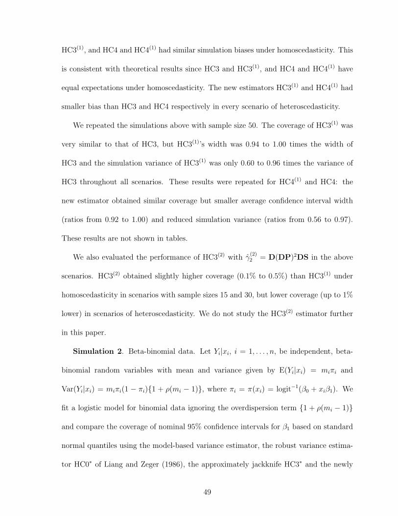
HC3(1), and HC4 and HC4(1) had similar simulation biases under homoscedasticity. This
is consistent with theoretical results since HC3 and HC3(1), and HC4 and HC4(1) have
equal expectations under homoscedasticity. The new estimators HC3(1) and HC4(1) had
smaller bias than HC3 and HC4 respectively in every scenario of heteroscedasticity.
We repeated the simulations above with sample size 50. The coverage of HC3(1) was
very similar to that of HC3, but HC3(1)’s width was 0.94 to 1.00 times the width of
HC3 and the simulation variance of HC3(1) was only 0.60 to 0.96 times the variance of
HC3 throughout all scenarios. These results were repeated for HC4(1) and HC4: the
new estimator obtained similar coverage but smaller average confidence interval width
(ratios from 0.92 to 1.00) and reduced simulation variance (ratios from 0.56 to 0.97).
These results are not shown in tables.
We also evaluated the performance of HC3(2) with γ(2)2 = D(DP)2DS in the above
scenarios. HC3(2) obtained slightly higher coverage (0.1% to 0.5%) than HC3(1) under
homoscedasticity in scenarios with sample sizes 15 and 30, but lower coverage (up to 1%
lower) in scenarios of heteroscedasticity. We do not study the HC3(2) estimator further
in this paper.
Simulation 2. Beta-binomial data. Let Yi|xi, i = 1, . . . , n, be independent, beta-
binomial random variables with mean and variance given by E(Yi|xi) = miπi and
Var(Yi|xi) = miπi(1 − πi){1 + ρ(mi − 1)}, where πi = π(xi) = logit−1(β0 + xiβ1). We
fit a logistic model for binomial data ignoring the overdispersion term {1 + ρ(mi − 1)}
and compare the coverage of nominal 95% confidence intervals for β1 based on standard
normal quantiles using the model-based variance estimator, the robust variance estima-
tor HC0∗ of Liang and Zeger (1986), the approximately jackknife HC3∗ and the newly
49

proposed HC3(1)∗ after 1000 simulations. We let β = {0, 1}T and choose the covariate
xi to be: (1) equally spaced in [-0.5, 0.5] so that πi is in (0.37, 0.63) and (2) equally
spaced in [-2, -1] so that πi is in (0.11, 0.27). The binomial denominators mi range
from 2 to 12 and are randomly selected from a truncated negative binomial distribution
with mean 3.12 and variance 4.12 similar to the U.S. sibship size distribution in 1950
(Brass, 1958; Donner and Koval, 1987). We explore the combinations of n = 25, 50 and
ρ = 0.1, 0.2, 0.3, 0.5. Results are shown in Table 3.3. It is clear that the binomial model-
based variance estimator loses coverage quickly for increasing values of ρ. The robust
variance estimator HC0∗ leads to undercoverage with n = 25. Both HC3∗ and HC3(1)∗
maintain appropriate coverage for every scenario. Even though HC3∗ and HC3(1)∗ are
derived from the binomial model, they seem to implicitly account for the overdispersion
of the data. The difference in width between HC3∗ and HC3(1)∗ was less than 0.5%
in every scenario and is not shown in tables. The main difference between HC3∗ and
HC3(1)∗ was a smaller observed variance of HC3(1)∗: the ratio of simulation variance of
HC3(1)∗ to HC3∗ ranged from 0.65 to 0.91 in every scenario.
Simulation 3. Poisson data with extra-Poisson variation. Let Yi|xi, i = 1, . . . , n be
independent random variables from a gamma-Poisson mixture with mean and variance
given by E(Yi|xi) = λi and Var(Yi|xi) = λi(1 + b), where λi = λ(xi) = exp(β0 + xiβ1).
We fit a log-linear model for Poisson data ignoring the extra-Poisson variation term
(1 + b) and compare the coverage of nominal 95% confidence intervals for β1 based on
standard normal quantiles using the model-based variance estimator, the robust variance
estimator HC0∗ of Liang and Zeger (1986), the approximately jackknife HC3∗ and the
newly proposed HC3(1)∗ after 1000 simulations. We let β = {0, 1}T and choose the
50
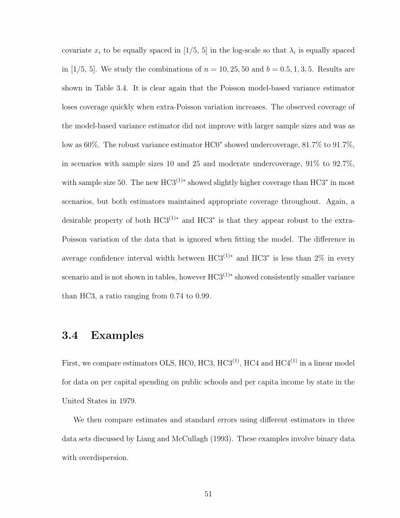
covariate xi to be equally spaced in [1/5, 5] in the log-scale so that λi is equally spaced
in [1/5, 5]. We study the combinations of n = 10, 25, 50 and b = 0.5, 1, 3, 5. Results are
shown in Table 3.4. It is clear again that the Poisson model-based variance estimator
loses coverage quickly when extra-Poisson variation increases. The observed coverage of
the model-based variance estimator did not improve with larger sample sizes and was as
low as 60%. The robust variance estimator HC0∗ showed undercoverage, 81.7% to 91.7%,
in scenarios with sample sizes 10 and 25 and moderate undercoverage, 91% to 92.7%,
with sample size 50. The new HC3(1)∗ showed slightly higher coverage than HC3∗ in most
scenarios, but both estimators maintained appropriate coverage throughout. Again, a
desirable property of both HC3(1)∗ and HC3∗ is that they appear robust to the extra-
Poisson variation of the data that is ignored when fitting the model. The difference in
average confidence interval width between HC3(1)∗ and HC3∗ is less than 2% in every
scenario and is not shown in tables, however HC3(1)∗ showed consistently smaller variance
than HC3, a ratio ranging from 0.74 to 0.99.
3.4 Examples
First, we compare estimators OLS, HC0, HC3, HC3(1), HC4 and HC4(1) in a linear model
for data on per capital spending on public schools and per capita income by state in the
United States in 1979.
We then compare estimates and standard errors using different estimators in three
data sets discussed by Liang and McCullagh (1993). These examples involve binary data
with overdispersion.
51

Example 1. This example is taken from Cribari-Neto (2004). The data appear in
Greene (1997, Table 12.1, p. 541). The response of interest yi is per capita spending
in dollars on public schools per state in 1979 in the United States. The covariate xi
is per capita income in dollars times 10−4. The state of Wisconsin is dropped from
all analyses due to missing response and Washington, DC is included. The state of
Alaska has very large recorded values for both income (1.0851) and spending (821) and
shows as a probable outlier in Figure 3.1. This results in very high leverage for Alaska,
hii = 0.651 ≈ 10p/n = 0.180. Interest lies on whether per capita income has a linear or
quadratic effect on spending. We follow the analysis of Cribari-Neto (2004) and fit the
model
yi = β0 + β1xi + β2x2i + εi
with and without Alaska. The parameter of interest is β2.
Table 3.7 shows estimates of β2 and corresponding standard errors using OLS, HC0,
HC3, HC3(1), HC4 and HC4(1). Table 3.7 shows that the OLS and HC0 estimators’
standard errors are noticeably smaller than those obtained with the other estimators.
Even though HC3 and HC3(1) have the same expected value under homoscedasticity,
this example shows that they can differ significantly in data analysis. The same holds
true for HC4 and HC4(1). The interpretation and statistical significance of β2 depends
on the choice of standard error and on whether Alaska is included in the analysis or
not. In both analyses with and without Alaska, HC3 appears to overcorrect the HC0
standard error when compared to HC3(1): corresponding standard errors for HC0, HC3
and HC3(1) are 829.99, 1995.24 and 1715.85 when including Alaska, and 626.68, 1103.03
52
and 1008.20 without Alaska. A similar situation arises with HC4 and the new HC4(1); the
HC4 estimator appears to overcorrect the HC0 standard error. The results in Simulation
1 lead us to prefer HC3(1) and HC4(1) over HC3 and HC4 respectively. Standard errors
obtained with HC4(1) are larger than HC3(1)’s but account for points of high leverage.
If the data have no points of high leverage, then HC3(1) is usually preferable to HC4(1).
This example shows the possible effect of a high influence point on parameter estimates
and standard errors. The estimators HC3(1) and HC4(1) appear less prone to overcorrect
the HC0 standard errors than HC3 and HC4 in these data.
Example 2. Liang and McCullagh (1993) studied the applicability of two models
for overdispersion in five data sets with binary responses from the literature. We revisit
three of their data sets applying their two models for overdispersion, robust variance
estimators based on their residuals, and a naive variance model.
The naive model is given by
Var(Yi) = miπi(1− πi)
where mi is the binomial denominator for Yi and πi is the probability of success. We
will refer to the naive model as Model 1.
Model 2 corresponds to a constant dispersion factor and is given by
Var(Yi) = miπi(1− πi)σ2.
53

Model 3 comes from the beta-binomial distribution and is given by
Var(Yi) = miπi(1− πi){1 + (mi − 1)ρ}
where ρ is the intra-class correlation parameter.
Table 3.5 shows parameter estimates and standard errors for three of the data sets
analyzed by Liang and McCullagh (1993). The first data set corresponds to a toxicol-
ogy study by Weil (1970) comparing two treatment groups, each with 16 observations.
The second data set is taken from Crowder (1978, Table 3). Crowder’s data address
the growth of 831 seeds divided into 21 batches. The third data set comes from a ter-
atological dietary study by Shepard, Mackler and Finch (1980) on 58 rats divided into
4 groups. Liang and McCullagh (1993) present a full description of these data sets.
We show standard errors based on the robust variance estimator HC0∗ and the newly
proposed HC3(1)∗ under the naive, constant dispersion and beta-binomial models. Note
that sandwich estimators obtained from the residuals of the naive model or residuals of
the constant dispersion model are equivalent.
Table 3.5 shows smaller standard errors obtained under the robust variance estimator
HC0∗ than the model based estimator in the three data sets. The HC3(1)∗ estimator helps
correct this behavior. However it is not clear which standard errors are ‘correct’ in any
given case.
To gain understanding of this problem we simulated beta-binomial data with the
same cluster setup and estimated parameters as those of Crowder’s data in Table 3.5.
54

The correlation ρ was set at its estimated valued ρ = 0.19. We fit the incorrect con-
stant dispersion model and corresponding HC0∗ and HC3(1)∗. Coverage of nominal 95%
confidence intervals based on these three estimators and normal quantiles after 10000
simulations is shown in Table 3.6. The new HC3(1)∗ shows coverage closer to nominal
than the constant correlation model and much closer than the robust variance estimator
HC0∗.
Table 3.5 shows that standard errors based on models for overdispersion and the
proposed HC3(1)∗ may differ significantly. In general, no one variance estimation method
works adequately for every scenario of binary data with overdispersion. It is possible
to devise situations where any of the estimators considered performs poorly. However,
the proposed HC3(1)∗ has been shown to be a competitive approach to model-based
overdispersion. It performs better than the commonly used robust variance estimator
HC0∗ in most scenarios and should be preferred to it, especially in small to medium
samples. It can help assess the appropriateness of an assumed dispersion model and
offers a viable alternative when no dispersion assumptions are made.
3.5 Discussion
We described a new class of variance estimators for regression models, and focused on
one member, HC3(1). The main motivation behind this estimator is that it has the same
expected value than HC3 under homoscedasticity, yet it has smaller variance. Based on
the new class of estimators, we defined HC4(1) as an alternative to the HC4 estimator of
55

Cribari-Neto (2004) for designs with high leverage points. The newly proposed estima-
tors differ from previously described estimators in that the estimate of the variance of
each observation is a linear combination of all the squared residuals, not only that obser-
vation’s squared residual. They thus seem to reduce variability by borrowing strength
across observations. We showed how the new class of estimators extends to generalized
linear models. The generalized HC3(1)∗ provides adequate inference in many situations
without the need for assumptions about the variance model. Our simulations show that
HC3(1)∗ provides intervals with coverage close to the nominal level in all but the most
extreme scenarios. Even when its coverage is similar to that of competing estimators
like HC3∗ , it shows consistently smaller variance and sometimes smaller average interval
width.
56

Table 3.1: Coverage of estimators OLS, HC3, HC3(1), HC4 and HC4(1)
n=15Model Distribution %Cover %Cover %Cover %Cover %Cover
OLS HC3 HC3(1) HC4 HC4(1) C8 C91 Exponential 98.00 94.70 96.50 96.80 99.50 1.04 0.501 Laplace 97.80 93.70 95.80 95.20 96.80 1.02 0.691 Normal 97.00 94.00 95.20 93.50 94.90 1.01 0.771 Uniform 97.00 95.80 96.00 94.70 95.20 1.00 0.862 Exponential 87.90 88.20 91.40 93.80 98.70 0.94 0.422 Laplace 91.70 95.20 96.50 96.70 97.70 0.96 0.632 Normal 94.80 94.90 95.80 94.90 95.80 0.98 0.712 Uniform 96.30 95.60 95.80 94.50 95.10 1.00 0.863 Exponential 80.70 90.40 90.60 95.00 98.90 0.91 0.423 Laplace 79.60 90.20 90.10 92.80 93.20 0.93 0.613 Normal 86.30 93.10 92.20 93.30 92.70 0.95 0.673 Uniform 93.20 94.40 94.30 93.20 93.30 0.99 0.84
n=30Model Distribution %Cover %Cover %Cover %Cover %Cover
OLS HC3 HC3(1) HC4 HC4(1) C8 C91 Exponential 95.60 93.30 94.30 95.20 97.30 1.02 0.621 Laplace 97.40 93.60 94.70 95.20 96.80 1.01 0.791 Normal 96.70 95.00 95.30 94.90 95.20 1.00 0.861 Uniform 96.60 95.80 96.00 95.60 95.80 1.00 0.952 Exponential 77.20 89.10 89.20 93.90 96.70 0.93 0.522 Laplace 84.40 95.40 95.00 97.10 97.70 0.96 0.722 Normal 92.50 93.50 93.60 93.40 93.90 0.99 0.822 Uniform 96.00 95.50 95.50 94.90 95.10 1.00 0.943 Exponential 73.40 90.90 89.80 95.40 96.60 0.92 0.513 Laplace 76.20 91.50 90.60 94.70 94.10 0.95 0.723 Normal 83.50 93.00 92.40 93.70 93.30 0.97 0.793 Uniform 94.00 95.50 95.60 95.30 95.20 0.99 0.92
* C8 = Width(HC3(1))/Width(HC3), C9 = Var(HC3(1))/Var(HC3)
Coverage, ratio of average widths and ratio of simulation variances refer to nominal95% confidence intervals of β1 after 1000 simulations. Model (1) is homoscedastic,and Models (2) and (3) are heteroscedastic as described in the text.
57

Table 3.2: Bias of estimators OLS, HC3, HC3(1), HC4 and HC4(1)
n=15Model Distribution %Bias %Bias %Bias %Bias %Bias
OLS HC3 HC3(1) HC4 HC4(1) C8 C91 Exponential 70.23 72.58 72.08 485.79 483.58 1.10 0.401 Laplace 41.37 44.72 43.88 81.60 80.40 1.02 0.641 Normal 33.77 30.94 31.65 32.53 33.35 1.02 0.731 Uniform 24.30 24.11 24.08 12.44 12.40 1.00 0.852 Exponential -43.22 41.24 11.01 483.62 334.73 0.94 0.362 Laplace -35.68 27.37 11.94 69.07 46.42 0.96 0.602 Normal -6.58 30.12 22.46 35.25 26.47 0.98 0.692 Uniform 19.77 22.51 22.13 11.00 10.65 1.00 0.853 Exponential -59.81 20.12 -8.67 391.92 251.72 0.91 0.363 Laplace -59.95 21.84 2.90 63.78 36.18 0.93 0.583 Normal -45.97 22.56 8.87 29.91 14.26 0.95 0.653 Uniform -10.89 17.61 13.66 7.01 3.31 0.99 0.84
n=30Model Distribution %Bias %Bias %Bias %Bias %Bias
OLS HC3 HC3(1) HC4 HC4(1) C8 C91 Exponential 27.89 26.22 26.51 123.79 124.57 1.05 0.501 Laplace 18.96 17.15 17.40 51.77 52.20 1.01 0.741 Normal 13.86 13.75 13.69 18.19 18.10 1.00 0.831 Uniform 11.38 10.44 10.51 5.32 5.40 1.00 0.942 Exponential -60.00 15.51 -5.54 164.64 105.94 0.92 0.462 Laplace -51.56 20.10 8.27 78.31 57.83 0.96 0.692 Normal -21.00 7.23 3.92 14.30 10.34 0.99 0.802 Uniform 8.34 10.45 10.27 5.41 5.23 1.00 0.933 Exponential -65.50 24.28 -0.64 187.50 118.22 0.91 0.453 Laplace -62.32 17.39 5.35 73.71 53.28 0.95 0.683 Normal -49.37 10.24 3.22 20.92 12.46 0.97 0.773 Uniform -13.75 11.46 9.50 6.74 4.83 0.99 0.91
* C8 = Width(HC4(1))/Width(HC4), C9 = Var(HC4(1))/Var(HC4)
Bias, ratio of average widths and ratio of simulation variances refer to nominal95% confidence intervals of β1 after 1000 simulations. Model (1) is homoscedastic,and Models (2) and (3) are heteroscedastic as described in the text.
58

Table 3.3: Confidence intervals fitting a logistic model for binomial data to beta-binomialdata
n=25Model ρ %Cover %Cover %Cover %Cover Var(HC3(1))
Var(HC3)Model HC0∗ HC3∗ HC3(1)∗
1 0.1 92.4 92.4 96.2 96.6 0.781 0.2 85.1 89.8 94.5 94.9 0.811 0.3 85.1 92.5 96.1 96.4 0.781 0.5 73.1 90.4 94.5 94.5 0.742 0.1 91.3 90.9 94.1 94.4 0.652 0.2 89.8 93.1 95.8 96.4 0.862 0.3 86.2 90.9 94.5 94.8 0.802 0.5 79.1 91.2 95.9 96.3 0.90
n=50Model ρ %Cover %Cover %Cover %Cover Var(HC3(1))
Var(HC3)Model HC0∗ HC3∗ HC3(1)∗
1 0.1 91.1 93.6 95.5 95.5 0.911 0.2 84.8 93.5 95.2 95.1 0.881 0.3 81.7 92.3 94.4 94.2 0.871 0.5 76.2 93.6 95.2 95.0 0.882 0.1 91.5 93.4 94.5 94.4 0.912 0.2 87.5 92.9 94.7 94.4 0.912 0.3 82.5 93.1 94.4 94.6 0.872 0.5 76.2 92.7 94.0 94.3 0.89
Nominal 95% confidence intervals of β1 after 1000 simulations.Estimators compared are the binomial model-based varianceestimator, the robust variance estimator HC0∗, the approxi-
mately jackknife HC3∗ and the newly proposed HC3(1)∗.
59

Table 3.4: Confidence intervals fitting a Poisson model to gamma-Poisson data
n b %Cover %Cover %Cover %Cover Var(HC3(1))Var(HC3)Model HC0∗ HC3∗ HC3(1)∗
10 0.5 91.5 86.6 94.1 96.0 0.9510 1 85.8 85.4 95.1 96.1 0.8610 3 76.1 85.2 95.9 97.0 0.7910 5 68.5 81.7 93.9 96.6 0.6225 0.5 90.3 90.7 94.7 94.9 0.9525 1 86.1 90.3 94.1 94.1 0.9525 3 71.5 89.8 93.7 94.4 0.9125 5 64.1 87.6 91.9 93.1 0.8550 0.5 88.9 92.4 93.7 93.7 0.9850 1 84.3 92.7 94.0 94.2 0.9750 3 71.1 91.9 93.6 93.6 0.9650 5 60.0 91.0 93.1 93.2 0.97
Nominal 95% confidence intervals of β1 after 1000 simulations.Estimators compared are the Poisson model-based varianceestimator, the robust variance estimator HC0∗, the approxi-
mately jackknife HC3∗ and the newly proposed HC3(1)∗.
60

Tab
le3.
5:A
nal
ysi
sof
over
dis
per
sed
bin
ary
dat
a
Wei
l-W
illia
ms’
Tox
icol
ogy
Dat
aD
ispe
rsio
nE
stim
ate
Stan
dard
Err
orM
odel
:1&
23
12
3M
odel
Mod
elH
C0∗
HC
3(1)∗
Mod
elH
C0∗
HC
3(1)∗
Inte
rcep
t2.
183
2.14
40.
264
0.43
20.
283
0.30
30.
437
0.28
40.
303
Tre
atm
ent
-0.9
61-1
.021
0.33
00.
541
0.47
50.
508
0.53
90.
471
0.50
2
Cro
wde
r’s
Ger
min
atio
nD
ata
Dis
pers
ion
Est
imat
eSt
anda
rdE
rror
Mod
el:
1&2
31
23
Mod
elM
odel
HC
0∗H
C3(1
)∗M
odel
HC
0∗H
C3(1
)∗
Inte
rcep
t-0
.558
-0.5
350.
126
0.17
20.
176
0.22
60.
194
0.17
80.
223
Roo
t1.
318
1.33
00.
178
0.24
20.
242
0.31
30.
278
0.23
80.
298
Seed
0.14
60.
070
0.22
30.
305
0.28
70.
384
0.31
20.
289
0.37
3R
oot*
Seed
-0.7
78-0
.819
0.30
60.
418
0.37
40.
501
0.43
50.
382
0.49
2
Shep
ard-
Mac
kler
-Fin
ch’s
Ter
atol
ogy
Dat
aD
ispe
rsio
nE
stim
ate
Stan
dard
Err
orM
odel
:1&
23
12
3M
odel
Mod
elH
C0∗
HC
3(1)∗
Mod
elH
C0∗
HC
3(1)∗
Inte
rcep
t1.
144
1.21
20.
129
0.21
90.
276
0.28
60.
223
0.26
90.
279
Gro
up2
-3.3
23-3
.370
0.33
10.
560
0.44
00.
477
0.56
30.
430
0.46
2G
roup
3-4
.476
-4.5
850.
731
1.23
80.
610
0.74
61.
303
0.62
40.
757
Gro
up4
-4.1
3-4
.250
0.47
60.
806
0.57
60.
646
0.84
80.
605
0.66
8
Est
imat
esan
dst
anda
rder
rors
are
obta
ined
usin
gM
odel
1:na
ive,
Mod
el2:
cons
tant
disp
ersi
on,
and
Mod
el3:
beta
-bin
omia
l,an
dco
rres
pond
ing
robu
stva
rian
cees
tim
ator
sH
C0∗
and
HC
3(1)∗
.
61

Table 3.6: Beta-binomial simulations based on Crowder’s data
%Coverage
Parameter Model HC0∗ HC3(1)∗
Intercept 90.71 84.06 90.94Root 89.85 87.39 93.84Seed 93.23 86.16 93.84
Root*Seed 92.30 88.02 95.73
Nominal 95% confidence intervals usingthe constant dispersion model, HC0∗ and
HC3(1)∗ after 1000 simulations.
Table 3.7: Analysis of Greene’s data
With Alaska, n=50 Without Alaska, n=49
β2 = 1587.04 β2 = −314.14
SE SE
OLS 716.38 OLS 872.60HC0 829.99 HC0 626.68HC3 1995.24 HC3 1103.03
HC3(1) 1715.85 HC3(1) 1008.20HC4 5488.93 HC4 2320.83
HC4(1) 4649.77 HC4(1) 2065.17
62

Figure 3.1: Per capita income and per capita spending in public schools
●●
●
●●
●
●
●
●
●
●
●●
●
●
●●
●
●
●
●
●
●●
●
●
●●
●
●
● ●
●●
●●
●
●
●
●
●
●
●
●
●
●
●
● ●
●
0.6 0.7 0.8 0.9 1.0 1.1
300
500
700
Income
Spe
ndin
g
63

Chapter 4
Variance estimation for correlated
data
4.1 Introduction
The generalized estimating equations (GEE) methodology (Liang and Zeger, 1986) fa-
cilitates the analysis of correlated and longitudinal data. GEE accounts for correlation
within subjects or clusters by specifying a working correlation model for observations
within a subject. The robust covariance estimator for GEE provides consistent esti-
mation of the true covariance matrix of the parameters of interest even if the working
correlation model is misspecified. However, it is known that the robust covariance esti-
mator may lead to anti-conservative inference when the number of independent subjects
or clusters is small (Mancl and DeRouen, 2001; Fay and Graubard, 2001; Lipsitz et al.,
1994).
Two main types of corrections have been proposed to improve the small sample
properties of inferential methods based on the robust variance estimator: bias-corrections

to the estimator itself and corrections to the degrees of freedom of the test statistic.
Corrections to the degrees of freedom of test statistics have met limited success (Fay
and Graubard, 2001; Lu et al., 2007; Braun, 2007). In this chapter we consider the bias
corrected robust variance estimators of Kauermann and Carroll (2001) and Mancl and
DeRouen (2001). These corrections obtain confidence intervals closer to nominal size in
small samples than the uncorrected robust variance estimator.
In Chapter 3, we proposed a class of robust variance estimators for independent
data that includes some currently available estimators and introduced new estimators
with reduced variance and improved confidence interval coverage. In this chapter, we
extend the class of variance estimators of Chapter 3 to generalized estimating equations.
The new class includes the estimators of Kauermann and Carroll (2001) and Mancl and
DeRouen (2001) as well as some new estimators. We follow a similar approach to Chapter
3 and show in simulations for correlated data that the newly proposed estimators have
smaller variance and better coverage than current estimators. This chapter is organized
as follows. In §4.2 we define the class of variance estimators in Chapter 3 in a recursive
manner. In §4.3 we define a class of variance estimators for GEE based on similar
recursive arguments. In §4.4 we present simulation studies; in §4.5 we show a data
analysis example. §4.6 is a conclusion.
4.1.1 Notation
Some of the notation used in this chapter was introduced in Chapter 1 and Chapter 3.
We require the following additional notation in this chapter: the matrix B = {A}diag
will denote the square matrix with diagonal elements bii = aii and bij = 0 if i 6= j. Let
65

C be a block matrix with block elements Cij, then blockdiag(C) will denote the block
diagonal matrix with block elements Cii.
4.2 Independent Data
Consider the linear model EY = Xβ,Var(Y) = Γ where Y is an n × 1 vector of
responses, X is a known n × p matrix of covariates of rank p, β is a p × 1 vector of
unknown parameters, and Γ = diag(γ1, . . . , γn) is unknown. In Chapter 3, we proposed
a class of estimators of cov(β) for independent data obtained by replacing Γ by Γ(k)
δ in
cov(β) = (XTX)−1XTΓX(XTX)−1.
We defined Γ(k)
δ = diag(γ(k)δ ) in vector form as
γ(k)δ = Dδ−1(DP)kDr∗2 (4.1)
where D = diag{1/(1 − hii)}, P = (I−H)∗2, r = Y − Y, k is an integer, δ ≥ 0,
H = X(XTX)−1XT and the operator A∗b denotes the b-th Schur power of A. Estimators
in this class are consistent for cov(β) for any fixed integer k and δ ≥ 0. The class in
(4.1) includes White’s estimator HC0 with Γ(0)0 , HC2 with Γ
(0)1 and HC3 with Γ
(0)2 . We
also discussed the HC4 estimator of Cribari-Neto (2004) for data sets with high leverage
points. The HC4 estimator does not belong to the class in (4.1), but it is closely related.
We proposed new estimators HC3(1) and HC4(1) and showed that they improve upon
HC3 and HC4 respectively in terms of confidence interval coverage and variance of the
66

variance estimators in many scenarios for linear models and generalized linear models in
small samples.
Variance estimators in (4.1) follow a recursive structure that allows a generalization
to correlated data. The result follows from the fact that Er∗2 = Pγ and therefore
Eγ(k−1)δ = Dδ−1(DP)k−1DPγ. This allows us to write estimators in (4.1) as:
γ(k)δ = Eγ
(k−1)δ |γ=γ(0)
1
= Dδ−1(DP)k−1DPγ|γ=γ(0)
1
= Dδ−1(DP)kDr∗2,
and in matrix form as
Γ(k)
δ = E(Γ(k−1)
δ )|Γ=
ˆΓ(0)
1
= diag(Dδ−1(DP)kDr∗2). (4.2)
Thus (4.2) defines Γ(k)
δ in terms of Γ(k−1)
δ and the HC2 variance estimator Γ(0)
1 , and
therefore the class of estimators in (4.1) is defined recursively. In the following sections,
the recursive property of Γ(k)
δ is extended to new variance estimators for generalized
estimating equations.
Finally, before discussing GEE, we write estimators Γ(k)δ , with k ≥ 0, in a form that
is easily generalizable to correlated data:
Γ(k)δ = {(Dδ−1(DP)kD)∗1/2diag(r∗2)(DT (PTDT )kD(δ−1)T )∗1/2}diag
= {(Dδ−1(DP)kD)∗1/2{rrT}diag(D(PD)kDδ−1)∗1/2}diag.
67

In particular, the case k = 0 simplifies to
Γ(0)δ = {Dδ/2{rrT}diagDδ/2}diag = {Dδ/2rrTDδ/2}diag. (4.3)
4.3 Correlated Data
We revisit some concepts of variance estimation for correlated data discussed in §1.4.4.
Consider a study with M total clusters and ni observations in the i-th cluster. Observa-
tions in the i-th cluster are indexed by yij, j = 1, . . . , ni. The response yij is related to
a p× 1 vector of covariates xij through g(µij) = xTijβ where µij = E(yij|xij). Let µi =
{µi1, . . . , µini}T and let the vector of all responses be written as Y = {YT1 , . . . ,Y
TM}T .
We define cov(Yi) = Γi and the block-diagonal matrix cov(Y) = Γ. GEE estimates of
β are obtained by solving
Uβ,GEE1 =M∑i=1
DTi V−1
i (Yi − µi) = 0
where Di = ∂µi/∂βT , Vi = diag(σ
12ijj)Ri(α)diag(σ
12ijj), Ri is a working correlation matrix
for corr(Yi) and σijj = Var(Yij). We stated that estimators of cov(β) are obtained by
replacing Γi by an estimator in
cov(β) =
(M∑i=1
DTi V−1
i Di
)−1( M∑i=1
DTi V−1
i ΓiV−1i Di
)(M∑i=1
DTi V−1
i Di
)−1
. (4.4)
The BC0, or robust variance estimator of cov(β), is obtained by replacing Γi by
(Γ(0)
0 )i := rirTi in (4.4) where ri = (yi − µi). Kauermann and Carroll (2001) and Mancl
68

and DeRouen (2001) introduced corrections to the BC0 estimator. The BC1 estimator
of Kauermann and Carroll (2001) is obtained by replacing
(Γ(0)
1 )i := (Ini −Hii)−1/2rir
Ti (Ini −Hii)
−T/2
in (4.4). The BC2 estimator of Mancl and DeRouen (2001) is obtained by replacing
(Γ(0)
2 )i := (Ini −Hii)−1rir
Ti (Ini −Hii)
−T .
The BC1 and BC2 estimators were proposed to improve the small sample properties
of the BC0 estimator. For correlated binary data, Lu et al. (2007) generally recommend
the use of BC2 over BC1 and BC0 in the construction of confidence intervals based on
standard normal quantiles.
The poor performance of BC0 in terms of confidence interval coverage in small sam-
ples can be attributed to its downward bias and its large variance compared to parametric
estimators. Kauermann and Carroll (2001) show that the large variance of the robust
or sandwich variance estimator causes undercoverage of confidence intervals in small
samples. In Chapter 3, we showed that sandwich estimators with Γ(1)δ defined in (4.1)
improve upon HC2 and HC3 estimators in terms of variance and confidence interval
coverage for independent data. In the following section, we use the results of §4.2 to
extend the family of variance estimators in (4.1) to correlated data.
69
4.3.1 A class of variance estimators for correlated data
Let D = blockdiag((Ii −Hii)−1) where Hij = DiS
−1DTj V−1
j and S =∑M
l=1 DlV−1l DT
l .
Note that Di are not components of D.
For any δ ≥ 0, we define a class of variance estimators for correlated data obtained
by replacing Γi in (4.4) by
Γ(0)δ := blockdiag(D
δ−12 D
12 blockdiag(rrT )D
12TD
δ−12T ) = blockdiag(D
δ2 rrTD
δ2T ).
These estimators are a generalization of the independent data variance estimators
Γ(0)δ defined in (4.1) and written in form (4.3). In particular, if δ = 0 we obtain BC0, if
δ = 1 we obtain Kauermann and Carroll’s estimator BC1 with
Γ(0)1 = blockdiag(D
12 rrTD
12T ).
If δ = 2 we obtain Mancl and DeRouen’s estimator BC2 with
Γ(0)2 = blockdiag(DrrTDT ).
In order to construct estimators Γ(k)δ with k > 0 for correlated data we propose a
recursive procedure analogous to the one described in §4.2. If k is a positive integer and
δ ≥ 0, we define:
Γ(k)δ = E(Γ
(k−1)δ )|
Γ=Γ(0)1. (4.5)
70

The expectation E(Γ(k−1)δ ) is evaluated using the approximation
E(rirTi ) ≈ (Ii −Hii)Γi(Ii −Hii)
T +∑j 6=i
HijΓjHTij (4.6)
given by Mancl and DeRouen (2001). This approximation allows a componentwise def-
inition of the recursive procedure in (4.5). Consider (Γ(k)δ )i, the estimator of cov(Yi)
given by the i-th block-diagonal element of Γ(k)δ . If k = 0 and δ = 1, we obtain the BC1
estimator with
(Γ(0)1 )i = (Ii −Hii)
− 12 rir
Ti (Ii −Hii)
− 12T .
We use (4.6) to obtain its approximate expectation
E(Γ(0)1 )i ≈ (Ii −Hii)
− 12
((Ii −Hii)Γi(Ii −Hii)
T +∑j 6=i
HijΓjHTij
)(Ii −Hii)
− 12T ,
and the recursive structure in (4.5) to define
(Γ(1)1 )i = E(Γ
(0)1 )i|Γj=(Γ
(0)1 )j ∀j=1,...,M
≈ (Ii −Hii)− 1
2
((Ii −Hii)(Γ
(0)1 )i(Ii −Hii)
T +∑j 6=i
Hij(Γ(0)1 )jH
Tij
)(Ii −Hii)
− 12T
= rirTi + (Ii −Hii)
− 12
(∑j 6=i
Hij(Ij −Hjj)− 1
2 rjrTj (Ij −Hjj)
− 12THT
ij
)(Ii −Hii)
− 12T .
The estimator (Γ(1)1 )i defined above is a generalization of the independent data
(γ(1)1 )i = r2
i +∑j 6=i
h2ij
(1− hii)(1− hjj)r2j
71
introduced in Chapter 3.
In general, estimators (Γ(1)δ )i can be written as
(Γ(1)δ )i = (Ii −Hii)
− δ−12 rir
Ti (Ii −Hii)
− δ−12T
+ (Ii −Hii)− δ
2
(∑j 6=i
Hij(Ij −Hjj)− 1
2 rjrTj (Ij −Hjj)
− 12THT
ij
)(Ii −Hii)
− δ2T .
Variance estimators BC1 and BC2 are obtained by replacing Γ by Γ(0)1 and Γ
(0)2 in
(4.4). We define two new variance estimators: BC1(1) and BC2(1), obtained by replacing
Γ by Γ(1)1 and Γ
(1)2 in (4.4) respectively. In the following sections we compare the perfor-
mance of BC1 and BC2 to that of BC1(1) and BC2(1) in simulations. We show that the
newly proposed estimators perform better in many scenarios in terms of variance and
coverage of confidence intervals.
The focus of this chapter is improved performance of variance estimators for corre-
lated data in small samples. However, it can be shown that the newly proposed variance
estimators BC1(1) and BC2(1) share the same large sample properties as BC1 and BC2.
A proof of consistency of BC1(1) and BC2(1) is shown in the appendix.
4.3.2 Computational issues
Let A be a n × n positive semidefinite matrix. We use the notation A12 to denote the
specific square root matrix defined via diagonalization as follows. Let A = VDVT be
the eigen-decomposition of A where V is the matrix of eigenvectors of A and D is the
diagonal matrix D = VTAV. Then A12 = VD
12 VT .
It would appear that for any δ ≥ 0, computation of estimators in the class Γ(1)δ
72

requires much more computational effort than Γ(0)δ since the new estimators involve
cross terms Hij, i 6= j. However, the terms Hij need not be calculated in estimators like
Γ(0)1 and Γ
(0)2 . In this section we show that the expression of Γ
(1)δ can be manipulated
so that its computation does not involve terms Hij, i 6= j. We use the fact that Hij =
DiS−1DT
j V−1j where S =
∑Ml=1 DlV
−1l DT
l .
In order to simplify Γ(1)δ , we use its componentwise form:
(Γ(1)δ )i = (Ii −Hii)
− δ−12 rir
Ti (Ii −Hii)
− δ−12T
+ (Ii −Hii)− δ
2
(∑j 6=i
Hij(Ij −Hjj)− 1
2 rjrTj (Ij −Hjj)
− 12THT
ij
)(Ii −Hii)
− δ2T .
The first term of (Γ(1)δ )i does not allow further simplification. The second term of
the sum can be written as
(Ii −Hii)− δ
2
(∑j 6=i
DiS−1DT
j V−1j (Ij −Hjj)
− 12 rjr
Tj (Ij −Hjj)
− 12TV−1
j DjS−1DT
i
)×
(Ii −Hii)− δ
2T
= (Ii −Hii)− δ
2 DiS−1
(∑j 6=i
DTj V−1
j (Ij −Hjj)− 1
2 rjrTj (Ij −Hjj)
− 12TV−1
j Dj
)×
S−1DTi (Ii −Hii)
− δ2T . (4.7)
Now let U :=(∑M
l=1 DTl V−1
l (Il −Hll)− 1
2 rlrTl (Il −Hll)
− 12TV−1
l Dl
). It follows that
(4.7) can be written as
(Ii −Hii)− δ
2 DiS−1(U−DT
i V−1i (Ii −Hii)
− 12 rir
Ti (Ii −Hii)
− 12TV−1
i Di
)×
S−1DTi (Ii −Hii)
− δ2T ,
73

and therefore we can write
(Γ(1)δ )i = (Ii −Hii)
− δ−12 rir
Ti (Ii −Hii)
− δ−12T
+ (Ii −Hii)− δ
2 DiS−1(U−DT
i V−1i (Ii −Hii)
− 12 rir
Ti (Ii −Hii)
− 12TV−1
i Di
)×
S−1DTi (Ii −Hii)
− δ2T .
This last form of (Γ(1)δ )i is computationally simpler since it does not involve any cross
terms Hij, i 6= j.
4.4 Simulations
We compare the performance of sandwich estimators of Var(zT β) of the form zT (covβ)z
in simulations for correlated data.
The first example concerns multivariate normal data with possibly misspecified work-
ing correlation structure. The second example deals with correlated binary data. For
each set of simulations we compare the newly proposed BC1(1) and BC2(1) with the esti-
mators BC1 of Kauermann and Carroll (2001), BC2 of Mancl and DeRouen (2001), the
uncorrected estimator BC0 and the naive or model-based variance estimator in terms of
interval coverage and variance.
Simulation 1. Multivariate normal data. We simulate yi from a multivariate normal
distribution with element-wise expected value Eyij = β0 + x1iβ1 + x2ijβ2 with β0 = 0,
β1 = 1 and β2 = 1 where x1 is a cluster level covariate generated from a standard normal
distribution and x2 varies within-cluster and is generated as (a) exponential with mean
74

1, (b) standard Laplace, (c) standard normal. We consider simulations with M = 10
and M = 20 independent clusters and common cluster size ni = 4. The cluster-level
correlation matrix is either exchangeable (XCH) with σ2 = 1 and ρ = 0.2 or has an
independence structure (I) with σ2 = 1. The working correlation matrix is independent
(I), exchangeable with ρ estimated from the data (XCH), or exchangeable with ρ = 0.2
fixed (True). Confidence intervals were constructed using quantiles of a t-distribution
with∑ni − 3 degrees of freedom. Simulation results are based on 2000 replicates.
Table 4.1 shows nominal 95% confidence intervals for β1 using the naive or model-based
variance estimator, the uncorrected BC0, BC1 of Kauermann and Carroll (2001), BC2
of Mancl and DeRouen (2001), BC1(1) and BC2(1). Table 4.2 shows corresponding 95%
confidence intervals for β2.
Table 4.1 and Table 4.2 show that the naive or model based variance estimator
provided adequate coverage for both β1 and β2 only when both the true correlation
and the working correlation had an independence structure, or both the true correlation
and the working correlation structures were exchangeable and ρ was fixed at its true
value. The scenarios with true independence or exchangeable structure and exchangeable
working correlation structure have a correctly specified correlation structure. These
scenarios show that in small samples, underestimation of association parameters can
affect the coverage of confidence intervals of mean parameters obtained by the model
based variance estimator even when the model is correct. Lu et al. (2007) suggest a bias
correction for estimated association parameters that improves the confidence coverage
of mean parameters based on the model, BC0 and BC1 variance estimators, and may
result in slight overcoverage of the BC2 estimator. Our simulation results show coverage
75
based on uncorrected mean and association parameter estimates.
The uncorrected robust variance estimator BC0, the BC1 estimator and BC1(1) pro-
duced varying levels of undercoverage of confidence intervals in every scenario, often
falling bellow 90%. The BC2 estimator improved upon BC0 and BC1 in terms of cov-
erage but still slightly undercovered the parameters of interest, with coverage close to
93% and 94% in most scenarios. The newly proposed BC2(1) obtained coverage closer to
nominal than any other estimator considered. The newly proposed BC2(1) and BC1(1)
led to equal or higher coverage than BC2 and BC1 respectively in every situation, while
maintaining comparable average interval width: the difference in average interval width
between BC2(1) and BC2 was less than 1% in most scenarios with a maximum differ-
ence of 4%. Differences in width are not shown in tables. The main difference between
the new estimators and BC2 and BC1 was the smaller observed variance of the new
estimators.
We repeated these simulations using autoregressive(1) (AR1) and moving average(1)
(MA1) true correlation structures and AR1, MA1, exchangeable and independence work-
ing correlation structures. The results were comparable to the ones presented in Table
4.1 and Table 4.2 in terms of coverage, width and variance of the estimators. These
results suggest that BC2 and BC2(1) may protect against misspecification of the work-
ing correlation structure in scenarios with a small number of clusters. Overall, the new
BC2(1) performed better than BC2 in terms of coverage and variance, and was com-
parable in terms of average width. We also repeated these simulations with M = 50
independent clusters. Results were qualitatively similar to the case M = 20, but the
difference in coverage and variance between estimators was smaller. The BC2(1) still
76

obtained coverage closer to nominal overall and smaller variance than BC2.
Simulation 2. Correlated binary data. We conducted a simulation study to evaluate
the performance of the newly proposed BC1(1) and BC2(1) with the estimators BC1 of
Kauermann and Carroll (2001) and BC2 of Mancl and DeRouen (2001) in a setting with
variable cluster sizes. Let us define µijk = pr(Yij = Yik = 1). The association between
Yij and Yik is represented by the odds ratio
ψijk =µijk(1− µij − µik + µijk)
(µij − µijk)(µik − µijk).
We generated correlated binary data from the models
logit(µij) = β0 + β1x1i + β2x2ij
and
log(ψijk) = α0 + α1|x1i|+ α2|x2ij − x2ik|
using the conditional linear family of Qaqish (2003). The covariate x1 is a cluster level
covariate generated from the standard normal distribution and x2 varies within-cluster
and is generated as (a) exponential with mean 1, (b) standard Laplace, (c) standard
normal.
Estimation was done using GEE1 for β with independence working correlation struc-
ture Ri(α) = I. The residuals ri obtained from these estimating equations were used to
construct variance estimators of β1 and β2 of the form aTBC(k)δ a with aT = {0, 1, 0} and
{0, 0, 1} respectively.
77

We fixed β = {−1, 0.4, 0.1}T and α = {0.1, 0.3,−0.2}T . This setup results in ψijk
between 0.4 and 2.7 for most realizations of x1i, x2ij and x2ik. Number of clusters was
evaluated at M = 10, 20 or 25. Cluster sizes were set to either common size ni = 4 or a
50/50 mixture of clusters sizes 4 and 14. Corresponding 95% nominal confidence intervals
were constructed using a t-distribution with∑ni − 3 degrees of freedom. Simulation
results are based on 1000 replicates and are summarized in Table 4.3.
Our conclusions are as follows. Simulations results show that confidence intervals
based on the naive variance estimator BC0, BC1 and BC1(1) may undercover the pa-
rameters of interest. This behavior is clearest in confidence intervals for β1 where the
number of clusters was 10 or 20 and cluster sizes were a 50/50 mixture of clusters sizes
4 and 14. The BC2 estimator of Mancl and DeRouen and the new BC2(1) provided
coverage closer to nominal in most scenarios. Confidence intervals obtained using the
new estimators BC1(1) and BC2(1) had approximately the same average width as BC1
and BC2 respectively in every scenario: the maximum difference in average width be-
tween BC2(1) and BC2 was less than 1.5%. The difference in widths between estimators
is not shown in tables. The new estimators showed smaller variance in every scenario
and consistently higher coverage overall. In these simulations, it appears that BC2(1)
outperforms all other estimators considered in terms of coverage and also outperforms
BC2 in terms of variance while maintaining comparable average width.
78

4.5 Example
We analyze data from a clinical trial of 59 epileptic patients carried out by Leppik et al.
(1985). The data appear in Thall and Vail (1990). An 8-week baseline seizure rate was
recorded for each patient in the trial. Patients were randomized to either the antiepileptic
drug progabide or a placebo and the number of seizures in two weeks periods of time
was recorded at four successive clinic visits.
We fit a model for clustered Poisson data with GEE to analyze the number of seizures
at the four visits after randomization. We use the same covariates as Thall and Vail
(1990): baseline seizure rate, calculated as the logarithm of 14
times the baseline seizure
rate, logarithm of age in years, indicators Trt for the progabide group and Visit4 for
the fourth clinic visit. Table 4.4 shows mean parameter estimates and standard errors
assuming (1) an exchangeable correlation structure and (2) an independence correla-
tion structure. Standard errors are calculated using the model-based variance estimator
(MB), the model-based variance estimator corrected for overdispersion using the de-
viance of the model (MB∗), the robust variance estimator BC0, the BC1 estimator of
Kauermann and Carroll (2001), the BC2 estimator of Mancl and DeRouen (2001) and
the newly introduced BC1(1) and BC2(1). Thall and Vail (1990) fit models with several
variance-covariance structures to these data; we present parameter estimates and stan-
dard errors for their model “11” using the robust variance estimator BC0. If we let Yit be
the number of seizures for patient i at time t then model “11” assumes Var(Yit) = αtEYit
and cov(Yit, Yiu) = 0.
Table 4.4 shows that parameter estimates and standard errors calculated with the
79

robust variance estimator BC0 were similar for the exchangeable correlation model and
the independence model. In this example, the corrected variance estimators BC1, BC1(1),
BC2 and BC2(1) led to larger standard errors than BC0 under both the exchangeable
and independence correlation models and the standard errors reported by Thall and
Vail (1990) under model 11. This result suggests that BC0 standard errors might be too
small for these data. In particular, standard errors for the covariates Trt and Base.Trt
increased significantly when estimated under BC1, BC1(1), BC2 or BC2(1). Inference on
the effect of progabide on seizures and its interaction with the baseline seizure rate may
be anti-conservative if based on BC0 standard errors; use of corrected variance estimators
seems warranted. Table 4.4 shows large discrepancies between the standard errors for Trt
and Base.Trt estimated under BC1 and BC1(1) and under BC2 and BC2(2) respectively.
Based on our simulation results on variance and coverage, we suspect that BC1 and BC2
might overinflate the standard errors of Trt and Base.Trt and that BC1(1) and BC2(2) may
be more reliable. The reverse situation occurs with the effect of the covariate Baseline:
the new estimators BC1(1) and BC2(1) suggest larger standard errors than BC1 and BC2.
Standard errors calculated under BC0, BC1, BC1(1), BC2 and BC2(1) are not necessarily
different even in small or medium samples: the standard errors for covariate Visit4 were
almost unchanged by the choice of variance estimator. The difference in standard errors
across sandwich variance estimators would be expected to decrease with larger sample
sizes. Based on the results of Lu et al. (2007) and the results in this chapter, we believe
BC2(1) standard errors are most appropriate for analysis of these data.
The progabide data show strong evidence of heteroscedasticity and extra-Poisson
variation. The sandwich estimators BC0, BC1, BC2, BC1(1) and BC2(1) are robust to
80
misspecification of the variance model and offer some protection against heteroscedastic-
ity and over-dispersion. However, these data also include at least one highly influential
subject, identified by id 207 in Thall and Vail (1990). Deletion of this subject changes
parameter estimates and standard errors. The goal of this example is to show differences
between the various sandwich variance estimators in real data. A more detailed discus-
sion of the progabide data and influential subjects can be found in Thall and Vail (1990).
4.6 Discussion
We introduced a new class of variance estimators for generalized estimating equations,
and focused on two estimators not previously mentioned in the literature, BC1(1) and
BC2(1). We showed in simulations that BC1(1) and BC2(1) are comparable in terms of
average width to BC1 and BC2 respectively, but that BC1(1) and BC2(1) show smaller
variance in most scenarios with a small number of clusters. The smaller variance of
BC1(1) and BC2(1) translates into higher confidence interval coverage than BC1 and BC2
respectively. These results are consistent with the theory developed by Kauermann and
Carroll (2001) on the variance of sandwich estimators and with similar results for variance
estimators for independent data in Chapter 3. They show that increased variance of
sandwich variance estimators often translates into loss of coverage.
In our simulations for correlated normal data, BC2(1) obtained higher coverage than
BC2 in every scenario due to BC2(1)’s smaller simulation variance and comparable av-
erage width. In every scenario, BC2(1) showed larger simulation variance and larger
average interval width than BC1(1) and BC0 respectively. The difference in confidence
81
interval coverage between BC2(1) and BC1(1) can therefore be attributed to the larger
width of intervals obtained by BC2(1). Lu et al. (2007) note that intervals based on
the BC2 estimator may be too conservative in small samples for clustered binary data.
In our simulation study for correlated normal data, intervals constructed using a t dis-
tribution and M − p degrees of freedom, instead of our choice of∑M
i ni − p, produce
slight subnominal coverage with BC1(1) and slight overcoverage with BC2(1). The use of
M − p degrees of freedom is common in the literature. Our work suggests that BC2(1)
is preferable to BC2, and BC1(1) to BC1 in most situations. We believe that BC2(1) is
preferable to BC1(1) in our simulation scenarios with intervals based on a t distribution
with∑M
i ni − p degrees of freedom. More work is necessary to discriminate between
BC2(1) and BC1(1) in more general settings. The distribution of test statistics and the
choice of degrees of freedom for different corrections of the sandwich estimator are topics
of interest in the literature, see for example Fay and Graubard (2001) and Pan and Wall
(2002).
We observed in our simulations for correlated normal data that it is possible for a
confidence interval based on BC0 to be wider than an interval based on BC1, and an
interval based on BC1 to be wider than one based on BC2. This occurred in fewer
than 0.5% of the simulated data sets with M = 10 clusters, and even less frequently
in simulations with M = 20. The widths of intervals in every simulated data set were
ordered as follows: BC2(1) > BC1(1) > BC0.
Our work shows that use of the standard robust variance estimator BC0 results in
anti-conservative standard errors in studies with a small number of independent clusters.
Even though this result is well known in the literature, the use of BC0 in studies with
82

small sample size is still common in many fields. We recommend the use of corrected
variance estimators for the analysis of clustered data with small or moderate number of
clusters; in particular, the BC2(1) estimator obtains adequate coverage in the scenarios
considered in this chapter. Further comparison of BC1(1) and BC2(1) might justify their
use in other settings.
83

Table 4.1: Multivariate normal data with common cluster size ni = 4. Variance estima-tion of cluster-level parameter.
M = 10Correlation Dist. %Coverage
True Work X2 ρ Naive BC0 BC1 BC1(1) BC2 BC2(1) C8 C9I I expo 0 95.7 82.7 89.2 91.3 93.8 95.5 0.76 0.62I I laplace 0 95.9 82.0 87.9 90.3 93.1 95.4 0.89 0.73I I normal 0 94.3 81.6 88.2 90.2 93.5 95.7 0.81 0.52I XCH expo -0.048 90.7 83.3 90.2 91.2 94.2 95.7 0.72 0.39I XCH laplace -0.050 89.7 81.6 87.1 89.3 92.5 95.0 0.79 0.66I XCH normal -0.050 90.7 82.7 88.6 90.7 93.8 95.7 0.84 0.80XCH I expo 0 87.9 82.5 88.4 90.0 92.7 94.7 0.76 0.65XCH I laplace 0 87.6 81.6 88.0 89.7 93.1 95.0 0.76 0.64XCH I normal 0 86.5 80.9 87.9 89.8 92.9 95.2 0.76 0.67XCH XCH expo 0.112 90.0 82.4 88.6 91.0 93.2 95.4 0.75 0.62XCH XCH laplace 0.114 90.0 81.5 88.4 90.0 93.2 95.7 0.82 0.82XCH XCH normal 0.110 89.6 82.5 88.2 89.4 92.9 95.0 0.93 0.91XCH True expo 0.2 97.3 84.9 90.3 92.8 94.8 97.4 0.71 0.46XCH True laplace 0.2 97.7 88.1 92.8 94.5 95.6 97.5 0.79 0.60XCH True normal 0.2 97.4 87.8 92.1 94.1 95.5 96.8 0.84 0.78
M = 20Correlation Dist. %Coverage
True Work X2 ρ Naive BC0 BC1 BC1(1) BC2 BC2(1) C8 C9I I expo 0 95.0 89.0 91.5 92.4 94.3 94.8 0.85 0.81I I laplace 0 95.6 89.5 91.7 92.7 93.9 94.7 0.86 0.80I I normal 0 95.5 87.9 91.3 92.3 93.7 95.0 0.84 0.79I XCH expo -0.025 93.1 89.7 92.4 93.2 94.5 95.5 0.87 0.79I XCH laplace -0.021 92.9 89.1 91.7 92.1 93.8 94.1 0.83 0.76I XCH normal -0.026 92.9 89.1 91.4 92.0 94.1 94.8 0.84 0.79XCH I expo 0 88.4 88.8 91.3 91.9 93.6 94.0 0.85 0.80XCH I laplace 0 89.1 88.7 91.4 92.5 94.0 94.7 0.86 0.83XCH I normal 0 87.3 88.7 91.8 92.5 94.3 95.0 0.84 0.80XCH XCH expo 0.156 92.5 88.0 91.1 91.8 93.2 94.2 0.82 0.71XCH XCH laplace 0.154 92.7 89.3 92.2 92.6 94.7 95.2 0.84 0.77XCH XCH normal 0.154 92.1 88.4 91.2 92.1 93.4 94.1 0.82 0.70XCH True expo 0.2 95.6 90.2 92.4 93.4 94.5 95.2 0.82 0.72XCH True laplace 0.2 95.4 91.2 93.5 94.1 95.1 95.9 0.88 0.85XCH True normal 0.2 95.5 90.8 93.1 93.8 95.0 95.7 0.85 0.79
* C8 = Var(BC1(1))/Var(BC1), C9 = Var(BC2(1))/Var(BC2)
Nominal 95% confidence intervals of β1 after 2000 simulations using the naive varianceestimator, BC0, BC1, BC1(1), BC2 and BC2(1).
84

Table 4.2: Multivariate normal data with common cluster size ni = 4. Variance estima-tion of subject-level parameter
M = 10Correlation Dist. %Coverage
True Work X2 ρ Naive BC0 BC1 BC1(1) BC2 BC2(1) C8 C9I I expo 0 95.4 86.6 90.2 91.2 93.2 94.9 0.86 0.72I I laplace 0 95.6 82.6 88.6 91.2 93.1 96.2 0.82 0.61I I normal 0 94.6 88.7 91.6 92.1 93.5 94.2 0.87 0.84I XCH expo -0.048 93.1 85.0 89.1 90.3 92.6 94.7 0.83 0.63I XCH laplace -0.052 93.5 80.2 86.0 88.6 91.0 94.7 0.80 0.48I XCH normal -0.049 93.3 86.6 89.6 90.0 92.2 93.1 0.86 0.81XCH I expo 0 95.2 87.0 90.6 92.2 94.1 95.6 0.85 0.76XCH I laplace 0 94.6 82.5 88.9 90.7 93.4 95.8 0.86 0.64XCH I normal 0 94.9 88.8 91.1 91.8 93.7 94.8 0.84 0.78XCH XCH expo 0.112 93.2 85.0 88.6 89.7 91.7 93.5 0.83 0.65XCH XCH laplace 0.113 94.2 80.7 88.0 90.1 92.7 95.1 0.79 0.61XCH XCH normal 0.110 95.2 88.3 90.8 91.4 93.3 94.1 0.89 0.85XCH True expo 0.2 97.8 90.4 93.1 94.2 95.8 96.7 0.84 0.61XCH True laplace 0.2 97.5 86.4 91.0 93.1 94.9 96.7 0.83 0.52XCH True normal 0.2 97.0 92.9 94.3 94.7 95.8 96.2 0.88 0.84
M = 20Correlation Dist. %Coverage
True Work X2 ρ Naive BC0 BC1 BC1(1) BC2 BC2(1) C8 C9I I expo 0 95.2 90.2 92.0 92.9 93.8 94.6 0.86 0.74I I laplace 0 95.6 86.8 90.7 92.6 93.9 95.8 0.82 0.65I I normal 0 95.4 92.2 93.4 93.6 94.5 94.7 0.93 0.92I XCH expo -0.023 93.7 88.8 90.7 91.3 92.4 92.8 0.82 0.71I XCH laplace -0.021 94.0 84.6 88.5 90.6 92.3 94.6 0.83 0.66I XCH normal -0.027 94.5 91.8 93.4 93.5 94.3 94.3 0.92 0.91XCH I expo 0 95.3 90.5 92.1 92.8 94.0 95.0 0.84 0.78XCH I laplace 0 95.4 87.2 90.7 92.2 93.6 95.0 0.85 0.67XCH I normal 0 95.1 92.1 93.4 93.8 94.9 95.2 0.91 0.90XCH XCH expo 0.152 94.4 89.2 91.4 91.9 93.0 93.5 0.85 0.75XCH XCH laplace 0.156 95.0 86.6 89.4 91.7 92.6 95.2 0.80 0.55XCH XCH normal 0.149 93.9 90.9 91.7 91.8 92.7 92.9 0.94 0.92XCH True expo 0.2 96.8 93.5 94.8 95.2 96.0 96.5 0.88 0.78XCH True laplace 0.2 95.6 88.0 90.9 92.9 93.5 95.3 0.77 0.57XCH True normal 0.2 95.6 93.5 94.3 94.5 95.2 95.4 0.94 0.93
* C8 = Var(BC1(1))/Var(BC1), C9 = Var(BC2(1))/Var(BC2)
Nominal 95% confidence intervals of β2 after 2000 simulations using the naive varianceestimator, BC0, BC1, BC1(1), BC2 and BC2(1).
85

Table 4.3: Variance estimation for correlated binary data
95% nominal confidence intervals for cluster-level parameter β1
Dist. %Coverage Var(BC1(1))Var(BC1)
Var(BC2(1))Var(BC2)M ni X2 Naive BC1 BC1(1) BC2 BC2(1)
10 4/14 expo 87.3 86.5 87.4 92.7 94.7 77.0 64.44/14 laplace 89.1 88.7 90.2 93.0 95.5 75.2 58.64/14 normal 89.0 87.0 89.1 92.8 94.8 71.3 41.3
20 4/14 expo 85.8 89.4 89.5 92.5 92.9 73.9 63.14/14 laplace 89.8 92.3 92.6 94.8 95.7 73.2 66.64/14 normal 88.3 89.5 89.6 92.4 93.1 77.1 71.3
25 4 expo 92.6 93.0 93.3 94.9 95.7 80.2 71.34 laplace 93.4 92.4 92.9 94.1 94.8 84.6 79.04 normal 94.8 94.1 94.4 95.1 95.4 83.7 79.1
95% nominal confidence intervals for subject-level parameter β2
Dist. %Coverage Var(BC1(1))Var(BC1)
Var(BC2(1))Var(BC2)M ni X2 Naive BC1 BC1(1) BC2 BC2(1)
10 4/14 expo 94.4 92.6 92.8 94.2 94.9 87.6 79.04/14 laplace 92.3 91.4 91.7 93.8 93.8 87.0 82.04/14 normal 93.9 92.4 92.8 95.2 95.4 86.9 80.1
20 4/14 expo 93.1 93.2 93.6 94.5 94.8 91.4 88.24/14 laplace 92.6 93.7 93.7 94.1 94.3 93.9 92.64/14 normal 93.1 94.4 94.6 95.7 96.0 91.5 87.1
25 4 expo 96.0 95.4 95.5 96.3 96.5 90.7 83.94 laplace 94.9 95.1 95.0 95.7 96.0 94.1 93.04 normal 95.7 94.8 94.9 95.7 95.9 91.9 86.3
Coverage and ratio of simulation variances refer to nominal 95% confidenceintervals after 1000 simulations.
86
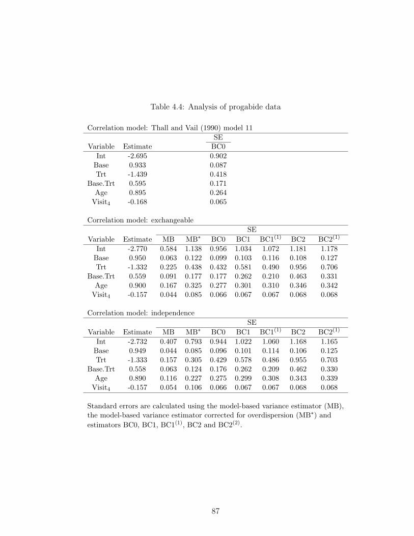
Table 4.4: Analysis of progabide data
Correlation model: Thall and Vail (1990) model 11SE
Variable Estimate BC0Int -2.695 0.902
Base 0.933 0.087Trt -1.439 0.418
Base.Trt 0.595 0.171Age 0.895 0.264
Visit4 -0.168 0.065
Correlation model: exchangeableSE
Variable Estimate MB MB∗ BC0 BC1 BC1(1) BC2 BC2(1)
Int -2.770 0.584 1.138 0.956 1.034 1.072 1.181 1.178Base 0.950 0.063 0.122 0.099 0.103 0.116 0.108 0.127Trt -1.332 0.225 0.438 0.432 0.581 0.490 0.956 0.706
Base.Trt 0.559 0.091 0.177 0.177 0.262 0.210 0.463 0.331Age 0.900 0.167 0.325 0.277 0.301 0.310 0.346 0.342
Visit4 -0.157 0.044 0.085 0.066 0.067 0.067 0.068 0.068
Correlation model: independenceSE
Variable Estimate MB MB∗ BC0 BC1 BC1(1) BC2 BC2(1)
Int -2.732 0.407 0.793 0.944 1.022 1.060 1.168 1.165Base 0.949 0.044 0.085 0.096 0.101 0.114 0.106 0.125Trt -1.333 0.157 0.305 0.429 0.578 0.486 0.955 0.703
Base.Trt 0.558 0.063 0.124 0.176 0.262 0.209 0.462 0.330Age 0.890 0.116 0.227 0.275 0.299 0.308 0.343 0.339
Visit4 -0.157 0.054 0.106 0.066 0.067 0.067 0.068 0.068
Standard errors are calculated using the model-based variance estimator (MB),the model-based variance estimator corrected for overdispersion (MB∗) andestimators BC0, BC1, BC1(1), BC2 and BC2(2).
87
Chapter 5
Summary and future research
5.1 Summary of accomplishments
5.1.1 Chapter 2: Random cluster size, within-cluster resam-
pling and generalized estimating equations
In Chapter 2 we discussed WCR for estimation of marginal parameters in correlated
binary data and WCPR for estimation of conditional parameters. We showed that
both WCR and WCPR can be thought of as specially weighted versions of generalized
estimating equations. We elaborated on the differences between WCR and unweighted
GEE in several models. We showed that the validity of WCR and unweighted GEE
is not dependent on cluster size ignorability, as had been previously claimed in the
literature, but rather that WCR and unweighted GEE estimate different parameters.
The validity of WCR and unweighted GEE depend on the model and the parameters
of interest of the study. We showed that the parameters estimated under WCPR have
some undesirable properties, such as being affected by the distribution of cluster sizes in

the sample and the exposure prevalence in the population. We proposed an alternative
estimating procedure based on generalized estimating equations with unit weights that
avoids some of the problems of WCPR, while having a similar interpretation.
5.1.2 Chapter 3: Variance estimation in regression models
We considered the problem of linear regression with heteroscedastic errors. The OLS
variance estimator is biased in this setting and the use of heteroscedasticity consis-
tent variance estimators is necessary. We reviewed robust variance estimators such as
the MINQUE, White’s HC0 (1980), HC1-HC3, and the HC4 estimator of Cribari-Neto
(1994). We proposed a new class of variance estimators that includes the MINQUE,
HC0, HC2, HC3 and the OLS as a limiting case. We showed that new robust variance
estimators in this class have smaller variance under homoscedasticity and many scenarios
of heteroscedasticity than HC0, HC2 and HC3. The new estimators show higher confi-
dence interval coverage in simulations in small samples while while maintaining average
interval width comparable to that of previously available estimators. We also proposed a
corrected version of the HC4 estimator with improved properties and extended the new
class of variance estimators to generalized linear models. In every case the newly pro-
posed variance estimators had smaller variance in simulations and improved confidence
interval coverage.
5.1.3 Chapter 4: Variance estimation for correlated data
We considered the problem of variance estimation for generalized estimating equations
and correlated data. The robust variance estimator BC0 of Liang and Zeger (1986) is too
89

liberal in studies with a small number of clusters. Corrected robust variance estimators
such as the BC1 and BC2 estimators of Mancl and DeRouen (2001) and Kauermann and
Carroll (2001) have been proposed to improve coverage in small samples. We generalized
the family of variance estimators introduced in Chapter 3 to GEE and correlated data.
We showed that the new family of variance estimators includes BC1 and BC2 as well as
new estimators. We showed that two new estimators in this family outperform BC1 and
BC2 in terms of confidence interval coverage and variance in simulations with correlated
binary data and multivariate normal data and showed an application to the progabide
data discussed by Thall and Vail (1990).
5.2 Future research
5.2.1 Robust variance estimation in other settings
Cox proportional-hazards model
The Cox proportional-hazards regression model (Cox, 1972) is widely used in survival
analysis. It is a popular tool to relate covariates with the distribution of survival times.
The proportional hazards assumption states a multiplicative relationship between the
hazard function and the log-linear function of the covariates. If the assumption of pro-
portional hazards holds, then the covariance matrix of the mean parameters can be con-
sistently estimated by the model-based variance estimator. Therneau (1999) identified
three kinds of diagnostics for Cox regression: violation of the assumption of proportional-
hazards, effect of influential data points, and nonlinearity in the model. Lin and Wei
90
(1989) proposed a variance estimator for the Cox proportional-hazards model that is ro-
bust against misspecification of the proportional-hazards assumption. The robust vari-
ance estimator of Lin and Wei (1989) shares the sandwich structure of the robust variance
estimator of Liang and Zeger (1986). In both types of variance estimators each subject’s
score function is added individually to obtain a sandwich-type variance estimator. We
believe it may be possible to extend the class of variance estimators in Chapter 3 and
Chapter 4 to Cox proportional-hazard models. The variance estimators derived in this
dissertation assign weights to each subject’s residual in a different way than the usual
robust variance estimator. We have shown that this strategy leads to reduced variance
and improved interval coverage in small samples in linear regression, generalized linear
models and GEE. We believe that a similar approach may improve the small sample
properties of sandwich estimators in proportional-hazard models when the assumption
of proportional-hazards is violated.
Finite population sampling
Robust variance estimation has been developed for linear regression in finite population
sampling by Royal and Cumberland (1978). Given a random sample from a finite pop-
ulation, Royal and Cumberland (1978) developed a variance estimator that is asymp-
totically equivalent to the jackknife and is robust to misspecification of the sample’s
variance model. Their variance estimator has a sandwich structure similar to that of the
HC0 estimator. We believe that the variance estimators proposed in Chapter 3 may be
extended to finite population sampling.
91

Association parameters
This dissertation has focused on variance estimation for mean parameters in various mod-
els. Sometimes interest lies in estimation of association parameters, such as intra-cluster
correlations in clustered binary data. Preisser, Lu and Qaqish (in preparation) compared
the BC0, BC1 and BC2 estimators for confidence interval coverage of intra-cluster cor-
relations in simulations. A natural extension of our work is to evaluate the performance
of new variance estimators for inference of association parameters for correlated binary
data.
5.2.2 Other topics
Degrees of freedom corrections
We mentioned in Chapter 4 that two main types of corrections aim to improve the
performance of robust variance estimators in small samples in correlated data in the
literature: corrections to the robust variance estimator itself and corrections to the
degrees of freedom of test statistics. Corrections to the robust variance estimator have
focused on bias reduction. We proposed variance-based corrections to the sandwich
variance estimator. Corrections to the degrees of freedom of test statistics have not been
successful in the literature (Lu et al., 2007; Braun, 2007). However, hybrid approaches
combining corrections to the variance estimator and the degrees of freedom of the test
statistic might offer improvements over current methodology. This topic of research has
been suggested by Pan and Wall (2003) and Braun (2007).
92

Outcome dependent sampling
Our work on WCR and WCPR resembles work in the literature on outcome dependent
sampling. Schildcrout and Heagerty (2005) studied the effect of design features on bias
and efficiency of GEE in the analysis of longitudinal binary data. They state that if
the model includes time dependent covariates, cross-sectional models may be biased un-
less the mean response is the same for multiple lagged values of the covariates or if an
independence correlation structure for GEE is used. This resembles statements on the
validity of WCR under informative cluster sizes. Schildcrout and Heagerty (2005) study
different working covariance models and their effect on bias and efficiency of parame-
ter estimates in this setting. Their work has parallels to our work on the validity of
unweighted GEE with informative cluster sizes. A review of the literature on outcome
dependent sampling may reveal connections to our work on resampling methods and
highlight future areas of research.
93

Appendix
A.2.1 Proof of results in the missing data model in §2.3.4.
Proof. Since
E[Ti|Ni > 0] =
n∗i∑k=1
Pr(Ni = k|Ni > 0)E[Ti|Ni = k]
=
n∗i∑k=1
Pr(Ni = k|Ni > 0)kpiγ1
piγ1 + (1− pi)γ0
=piγ1
piγ1 + (1− pi)γ0
E[Ni|Ni > 0],
it follows that
E[Ti|Ni > 0]
E[Ni|Ni > 0]=
piγ1
piγ1 + (1− pi)γ0
.
Similarly
E[TiNi
|Ni > 0] =
n∗i∑k=1
Pr(Ni = k|Ni > 0)E[TiNi
|Ni = k]
=
n∗i∑k=1
Pr(Ni = k|Ni > 0)1
kk
piγ1
piγ1 + (1− pi)γ0
=piγ1
piγ1 + (1− pi)γ0
n∗i∑k=1
Pr(Ni = k|Ni > 0)
=piγ1
piγ1 + (1− pi)γ0
.
Therefore
E[Ti|Ni > 0]
E[Ni|Ni > 0]= E[
TiNi
|Ni > 0].
94

This completes the proof.
A.3.1 Proof that limk→∞γ(k)1 = 1
n−pJS, the OLS estimator.
Proof. For simplicity, let us write (DP)∞ := limk→∞(DP)k. We want to prove that
(DP)∞D = 1n−pJ.
The matrix DP has diagonal elements (1− hii) and off-diagonal elements h2ij/(1− hii).
Hence the sum of the elements on its i-th row is equal to 1:
n∑j=1
(DP)ij = (1− hii) +∑j 6=i
h2ij
1− hii= 1.
It follows that DP1 = 1, where 1 is a vector with all elements equal to 1, and therefore
DP is a transition matrix.
Proving that (DP)∞D = 1n−pJ is equivalent to proving that the transition matrix DP
has limiting distribution 1n−pJD−1, also equivalent to showing that 1
n−pJD−1(DP) =
1n−pJD−1.
By properties of the hat matrix H,∑
j Pij = 1 − hii, and JD−1 = JP. It follows that
1n−pJD−1(DP) = 1
n−pJP = 1n−pJD−1 which completes the proof.
A.3.2 Proof of Property 1 in §3.2.3.
Proof. In order to prove that E(γ(k)1 ) = γ under homoscedasticity, write
E(γ(k)1 ) = (DP)kDE(S) = (DP)kDPγ = (DP)k+11σ2.
95

We proved in A.3.1 that DP is a transition matrix, it follows that (DP)k+1 is also a
transition matrix and therefore (DP)k+11σ2 = 1σ2.
A.3.3 Proof of Theorem 3.1.
Proof. Let the k-th Schur power (Marcus and Minc, 1964, p.120) of a vector or matrix
B = (bij) be defined as B∗k = (bkij).
The estimator zTΓ(k)δ z can be written as
zTΓ(k)δ z = (zT )∗2γ
(k)δ = uTδ (DP)kDS
where uTδ = (zT )∗2Dδ−1. Therefore we can write:
Var(zTΓ(k+1)δ z) = uTδ (DP)k+1DVar(S)D(PD)k+1uδ
and
Var(zTΓ(k)δ z) = uTδ (DP)kDVar(S)D(PD)kuδ.
Proving that Var(zTΓ(k+1)δ z) ≤ Var(zTΓ
(k)δ z) is equivalent to proving that
Var(zTΓ(k+1)δ z)
Var(zTΓ(k)δ z)
≤ 1 for all z.
From the expressions of Var(zTΓ(k)δ z) and Var(zTΓ
(k+1)δ z) above, it suffices to show that
C := ((DP)kDVar(S)D(PD)k)−1(DP)k+1DVar(S)D(PD)k+1
96

has all eigenvalues less than or equal to 1.
Under normality and homoscedasticity, Var(S) = 2σ4(I−H)∗2 = 2σ4P. In general, if
Var(S) ∝ P we can write
C = ((DP)kDPD(PD)k)−1(DP)k+1DPD(PD)k+1
= ((PD)k)−1(PD)kPDPD = PDPD.
Finally, we have shown before that DP is a strictly positive transition matrix: DP1 = 1
and (DP)ij > 0. Therefore CT = DPDP is also a strictly positive transition matrix.
Hence C has one eigenvalue equal to 1 and the remaining eigenvalues less than or equal
to 1. This completes the proof.
A.3.4 Proof of Property 3 in §3.2.3.
Proof. Dorfman (1991) proved this property for the case k = 0. The case k = 0 requires
regularity conditions of the leverages hii, in particular, that max1≤i≤n(hii) → 0 as n →
∞. To extend the proof to other values of k we need conditions under which ||(DP)k −
In|| → 0 as n→∞ for fixed k. Again the sufficient condition is that max1≤i≤n(hii)→ 0
as n→∞. Since (DP)k is a transition matrix it follows that ||(DP)k−In||2 = ||(DP)k−
In||∞ = 0. Regularity of the leverages guarantees that the max norm ||DP− In||max =
max1≤i≤n(hii)→ 0.
A.3.5 Proof of Theorem 3.2.
97

Proof. Let R be the vector of residuals ri, then R ∼ N(0, (I−H)Γ(I−H)).
Evaluating (I−H)Γ(I−H) under homoscedasticity, and by properties of H, we obtain
that Var(ri) = σ2(1− hii) and Cov(ri, rj) = −hijσ2.
Using fourth order moments of the multivariate normal distribution we obtain Cov(r2i , r
2j ) =
2Cov(ri, rj)2 and Var(r2
i ) = 2Var(ri)2. So that Corr(r2
i , r2j ) = h2
ij/(1 − hii)(1 − hjj) =
(DPD)ij if i 6= j and (DPD)ii = 1.
A.4.1
Liang and Zeger (1986) showed that under regularity conditions, BC0p−→ cov(β) as
M →∞, where cov(β) is given in (4.4). The necessary conditions are sufficient moments
of X, Y and smoothness of g(µi). If these conditions hold then max(ij)||Hij|| = O(M−1).
This follows from Hij = Di
(∑Ml=1 DT
l V−1l Dl
)−1
DTj V−1
j ; the norm
||(∑M
l=1 DTl V−1
l Dl
)−1
|| = O(M−1) while the rest of the terms in Hij are O(1).
Theorem 4.1 If regularity conditions are met such that max(ij)||Hij|| = O(M−1) then
BC1, BC1(1), BC2 and BC2(1) are consistent for cov(β) as M →∞.
Proof. Liang and Zeger (1986) showed that substituting Γi in (4.4) by (Γ(0)
0 )i = rirTi
guarantees convergence of BC0 as long as E(rirTi ) = Γi{1+O(M−1)}. This follows from
E(rirTi ) = (Ii −Hii)Γi(Ii −Hii)
T +∑j 6=i
HijΓjHTij +O(M−2)
as long as ||Hij|| = O(M−1) for all {i, j}.
We want to prove that (Γ(0)
1 )i, (Γ(0)
2 )i, (Γ(1)
1 )i and (Γ(1)
2 )i share the same asymptotic
98

expectation as (Γ(0)
0 )i. This result follows directly from the structure of these estimators:
(Γ(0)
1 )i = (Ini −Hii)−1/2rir
Ti (Ini −Hii)
−1/2T
(Γ(1)1 )i = rir
Ti
+ (Ii −Hii)− 1
2
(∑j 6=i
Hij(Ij −Hjj)− 1
2 rjrTj (Ij −Hjj)
− 12THT
ij
)(Ii −Hii)
− 12T
(Γ(0)
2 )i = (Ini −Hii)−1rir
Ti (Ini −Hii)
−1T
(Γ(1)2 )i = (Ii −Hii)
− 12 rir
Ti (Ii −Hii)
− 12T
+ ((Ii −Hii)−1
(∑j 6=i
Hij(Ij −Hjj)− 1
2 rjrTj (Ij −Hjj)
− 12THT
ij
)(Ii −Hii)
−1T .
If max(ij)||Hij|| = O(M−1) then (Γ(k)
δ )i = rirTi + O(M−1) for δ = 1, 2, k = 0, 1 and
therefore
E(Γ(k)
δ )i = Γi +O(M−1) δ = 1, 2 k = 0, 1
Then, by the arguments of Liang and Zeger (1986), BC1, BC1(1), BC2 and BC2(1) are
consistent for cov(β) as M →∞.
99

References
Bera, A. K., Suprayitno, T. and Premaratne, G. (2002). On some heteroskedasticity-robust estimators of variance-covariance matrix of the least-squares estimators. Jour-nal of Statistical Planning and Inference 108, 121-136.
Benhin, E., Rao, J.N.K. and Scott, A.J. (2005). Mean estimating equation approachto analysing cluster-correlated data with nonignorable cluster sizes. Biometrika 92,435-450.
Brass, W. (1958). Models of birth distribution in human populations. Bulletin of theInternational Statistical Institute 36, 165-167.
Braun, T.M. (2007). A mixed model-based variance estimator for marginal model anal-yses of cluster randomized trials. Biometrical Journal 49, 394-405.
Breslow, N.E. and Day, N.E. (1980). Statistical Methods in Cancer Research, Volume1, The Analysis of Case-Control Studies. Lyon: International Agency for Researchon Cancer.
Chesher, A. D. and Jewitt, I. D. (1987). The bias of a heteroskedasticity consistentcovariance-matrix estimator. Econometrica 55, 1217-1222.
Cong, X.J., Yin, G. and Shen, Y. (2007). Marginal analysis of correlated failure timedata with informative cluster sizes. Biometrics 63 663-672.
Cox, D.R. (1958). The regression analysis of binary sequences. Journal of the RoyalStatistical Society 20, 215-242.
Cox, D.R. (1972). Regression models and life tables. Journal of the Royal StatisticalSociety Series B 34, 187-220.
Cribari-Neto, F. (2004). Asymptotic inference under heteroskedasticity of unknownform. Computational Statistics and Data Analysis 45, 215-233.
Cribari-Neto, F., Ferrari, S.L.P. and Cordeiro, G.M. (2000). Improved heteroscedasticity-consistent covariance matrix estimators. Biometrika 87, 907-918.
Crowder, M.J. (1978). Beta-binomial ANOVA for proportions. Applied Statistics 27,34-37.
100
Datta, S. and Satten, G.A.(2005). Rank-sum tests for clustered data. Journal of theAmerican Statistical Association 100, 908-915.
Datta, S. and Satten, G.A. (2007) A signed-rank test for clustered data. Biometrics(Online Early Articles). doi:10.1111/j.1541-0420.2007.00923.x
Donner, A. and Koval, J.J. (1987). A procedure for generating group sizes from a one-way classification with a specified degree of imbalance. Biometrical Journal 29,181-187.
Dorfman, A.H. (1991). Sound coverage intervasl in the heteroscedastic linear modelthrough releveraging. Journal of the Royal Statistical Society: Series B (Method-ological) Ser. B 53, 441-452.
Eicker, F. (1963). Asymptotic normality and consistency of the least squares estimatorsfor families of linear regressions. The American Statistician 34, 447-456.
Faes, C., Hens, N., Aerts, M. and Shkedy, Z. (2006). Estimating herd-specific force ofinfection by using random-effects models for clustered binary data and monotonefractional polynomials. Journal of the Royal Statistical Society: Series C (AppliedStatistics) 55, 595-613.
Fay, M.P. and Graubard, B.I. (2001). Small-sample adjustments for Wald-type testsusing sandwich estimators. Biometrics 57, 1198-1206.
Flachaire, E. (2005). Bootstrapping heteroskesdastic regression models: wild bootstrapvs. pairs bootstrap. Computational Statistics and Data Analysis 49, 361-376.
Follmann, D., Proschan, M. and Leifer, E. (2003). Multiple outputation: inference forcomplex clustered data by averaging analysis from independent data. Biometrics59, 420-429.
Gansky, S.A., Weintraub, J.A., Shain, S., and the Multi-Pied Investigators (1998).Parental periodontal predictors of oral health in adult children of a community co-hort. Journal of Dental Research 77, (Special Issue B) 707.
Gansky, S.A., Weintraub, J.A., Shain, S., and the Multi-Pied Investigators (1999). Fam-ily aggregation of periodontal status in a two-generation cohort. Journal of DentalResearch 78, (Special Issue B) 123-132.
Greene, W.H. (1997). Econometric Analysis, 3rd Edition. Prentice-Hall, Upper SaddleRiver, NJ.
101

Hartley, H.O., Rao, J.N.K. and Kiefer, G. (1969). Variance estimation with one unit perstratum. Journal of the American Statistical Association 64, 841-851.
Hinkley, D.V. (1977). Jackknifing in unbalanced situations. Technometrics 19, 285-292.
Hoaglin, D.C. and Welsch, R. (1978). The hat matrix in regression and ANOVA. TheAmerican Statistician 32, 17-22.
Hoffman, E., Sen, P.K. and Weinberg, C.R. (2001). Within-cluster resampling. Biometrika88, 1121-1134.
Horn, S.D., Horn, R.A. and Duncan, D.B. (1975). Estimating heteroscedastic variancesin linear models. Journal of the American Statistical Association 70, 380-385.
Huber, P.J. (1967). “The behavior of maximum likelihood estimation under nonstan-dard conditions” in Proceedings of the Fifth Berkeley Symposium on MathematicalStatistics and Probability 1, eds. L. M. LeCam and J. Neyman, Berkeley: Universityof California Press, pp. 221-233.
Kauermann, G. and Carroll, R.J. (2001). A note on the efficiency of sandwich covariancematrix estimation. Journal of the American Statistical Association 96, 1387-1396.
Kuk, A.Y.C. (2003). A generalized estimating equation approach to modelling foetalresponse in developmental toxicity studies when the number of implants is dosedependent. Journal of the Royal Statistical Society: Series C (Applied Statistics)52, 51-61.
Laird, N.M. and Ware, J.H. (1982). Random-effects models for longitudinal data. Bio-metrics 38, 963-974.
Leppik, I.E. et al. (1985). A double-blind crossover evaluation of progabide in partialseizures. Neurology 35, 285.
Liang, K.Y. and McCullagh, P. (1993). Case studies in binary dispersion. Biometrics49, 623-630.
Liang, K.Y. and Zeger, S.L. (1986). Longitudinal data analysis using generalized linearmodels. Biometrika 73, 13-22.
Lin, D.Y. and Wei, L.J. (1989). The robust inference of the Cox proportional hazardsmodel. Journal of the American Statistical Association 84, 1074-1088.
102
Lipsitz, S.R., Fitzmaurice, G.M., Orav, E.J., and Laird, N.M. (1994). Performance ofgeneralized estimating equations in practical situations. Biometrics 50, 270-278.
Long, J.S. and Ervin, L.H. (2000). Using heteroscedasticity consistent standard errorsin the linear regression model. The American Statistician 54, 217-224.
Lu, B., Preisser, J.S., Qaqish, B.F., Suchindran, C., Bangdiwala, S.I. and Wolfson,M. (2007) A comparison of two bias-corrected covariance estimators for generalizedestimating equations. Biometrics 63, 935941.
MacKinnon, J.G. and White, H. (1985). Some heteroskedasticity consistent covariancematrix estimators with improved finite sample properties. Journal of Econometrics29, 205-325.
McCaffrey, D.F. and Bell, R.M. (2006). Improved hypothesis testing for coefficientsin generalized estimating equations with small samples of clusters. Statistics inMedicine 25, 4081-4098.
Mancl, L.A. and DeRoeun, T.A. (2001). A covariance estimator for GEE with improvedsmall-sample properties. Biometrics 57, 126-134.
Marcus, M. and Minc, H. (1964). A survey of matrix theory and matrix inequalities.Boston: Prindle, Weber and Schmidt.
McCullagh, P. & Nelder, J. (1989). Generalized Linear Models. CHAPMAN & HALL/ CRC, Boca Raton.
Miller, R.G. (1974). An unbalanced jackknife. Annals of Statistics 2, 880-991.
Morel, J.G., Bokossa, M.C. and Neerchal, N.K. (2003). Small correction for the varianceof GEE estimators. Biometrical Journal 45, 395-409.
Neuhaus, J.M., Hauck, W.W. and Kalbfleisch, J.D. (1992). The effects of mixture dis-tribution misspecification when fitting mixed-effects logistic models. Biometrika 79,755-762.
Neuhaus, J.M. and McCulloch, C.E. (2006). Separating between- and within-clustercovariate effects by using conditional and partitioning methods. Journal of the RoyalStatistical Society: Series B (Methodological) Ser.B 68, 859-872.
Pan, W. and Wall, M.M. (2002). Small-sample adjustments in using the sandwich vari-ance estimator in generalized estimating equations. Statistics in Medicine 21, 1429-1441.
103

Preisser, J.S. and Qaqish, B.F. (1996). Deletion diagnostics for generalized estimatingequations. Biometrics 83, 551-562.
Qaqish, B.F. (2003). A family of multivariate binary distributions for simulating corre-lated binary variables with specified marginal means and correlations. Biometrika90, 455-463.
Qian, L. and Wang S. (2001). Bias-corrected heteroscedasticity robust covariance matrix(sandwich) estimators. Journal of Statistical Computation & Simulation 70, 161-174.
Rao, C.R. (1970). Estimation of Heteroscedastic Variances in Linear Models. Journalof the American Statistical Association 65, 161-172.
Rasch, G. (1961). On general laws and the meaning of measurement in psychology.Pp. 321-333 in Proc. 4th Berkeley Symposium on Mathematics, Statistics, andProbability, Vol. 4, ed. J. Neyman. Berkeley, CA: University of California Press.
Rieger, R.H., Kaplan, N.L and Weinberg, C.R. (2001). Efficient use of siblings in testingfor linkage and association. Genetic Epidemiology 20, 175-195.
Rieger, R.H. and Weinberg, C.R. (2002). Analysis of clustered binary outcomes usingwithin-cluster paired resampling. Biometrics 58, 332-341.
Royal, R.M. and Cumberland, W.G. (1978). Variance estimation in finite populationsampling. Journal of the American Statistical Association 73, 351-358.
Schildrout, J.S. and Heagerty, P.J. (2005). Regression analysis of longitudinal binarydata with time-dependent environmental covariates: bias and efficiency. Biostatistics6, 633-652.
Shepard, T.H., Mackler, B., and Finch, C.A. (1980). Reproductive studies in the iron-deficient rat. Teratology 22, 329-334.
Shin, J., Darlington, A., Cotton, C., Corey, M. and Bull, S.B. (2007). Confidenceintervals for candidate gene effects and environmental factors in population-basedassociation studies of families. Annals of Human Genetics 71, 421-432.
Stiratelli, R., Laird, N. M. and Ware, J.H. (1984). Random-effects models for serialobservations with binary response. Biometrics 40, 961-971.
Thall, P.F. and Vail, S.C. (1990). Some covariance models for longitudinal count datawith overdispersion. Biometrics 46, 657-671.
104

Therneau, T.M. (1999). A package for survival analysis in S. Technical report.http://www.mayo.edu/hsr/people/therneau/survival.ps Mayo Foundation.
Weil, C.S. (1970). Selection of the valid number of sampling units and a considerationof their combination in toxicological studies involving reproduction, teratogenesis orcarcinogenesis. Food and Cosmetics Toxicology 8, 177-182.
White, H. (1980). A heteroskedasticity-consistent covariance matrix estimator and adirect test for heteroskesdasticity. Econometrica 48, 817-38.
Williamson, J.M., Datta, S. and Satten, G. A. (2003). Marginal analyses of clustereddata when cluster size is informative. Biometrics 59, 36-42.
Williamson, J.M., Kim, H.Y., Manatunga, A. and Addiss, D.G. (in press). Modeling sur-vival data with informative cluster size. Statistics in Medicine doi: 10.1002/sim.3003.
Williamson, J.M., Kim, H.Y. and Warner, L. (2007). Weighting condom use data toaccount for nonignorable cluster size. Annals of Epidemiology 17, 603-607.
Wu, C.F.J. (1986). Jackknife, bootstrap and other resampling methods in regressionanalysis. Annals of Statistics 14, 1261-1295.
Zeger, S.L. and Liang, K.Y. (1986). Longitudinal data analysis for discrete and contin-uous outcomes. Biometrics 42, 121-130.
105