estimate attrition using survival analysis
TRANSCRIPT

Estimating Insurance Attrition Using Survival Analysis
Luyang Fu, Ph.D., FCAS
CAS Spring Meeting, May 2015,
The author’s affiliation with The Cincinnati Insurance Company is provided for identification purposes only and is not intended to convey or imply The Cincinnati Insurance Company’s concurrence with or support for the positions, opinions or viewpoints expressed.

Agenda
• Introduction• Survival Analysis• Cox Proportional Hazard Model • A Case Study• Q&A

IntroductionAttrition/retention is important to insurance companiesGrowth (Top Line)
• “We were not successful in raising customer renewal rates, so that the new business success did not result in overall growth this quarter”
All State 2010Q4 Earnings call
• Higher retention, less pressure of attracting new business
To grow a book with 10,000 policies by 10%, – if retention is 90%, need to attract 2000 new accounts: 1000 to make up attrition, 1000
for the growth– if retention is 70%, need to write 4000 new accounts: 3000 to make up attrition, 1000
for the growth

IntroductionAttrition/retention is important to insurance companiesProfitability (Bottom Line)
• “Given our strong retentions as well as the new business and account growth we've achieved over the last few years, we have significant positive leverage to an improving environment.”
Travelers 2010Q4 Earning call
• Ageing Phenomenon – D’Arcy and Doherty (1989; 1990): loss ratio improves with policy age– Wu and Lin (2009): renewal book on average has a loss ratio 13% better than new
business by examining 8 lines of business, 25 books, $29 billion premium
• Price Optimization– Retention, conversion, price elasticity – Life-time value

IntroductionTwo types of Attritions• Mid-term cancellation• End-term nonrenewal
0 10 20 30 40 50 60
0.02
0.04
0.06
0.08
0.10
0.12
Policy Age: Month
Prob
abili
ty
Probability of Attrition: Cancellation vs. Nonrenewal

Introduction
Two types of attritions behave differently• Example 1: price elasticity
– End-term nonrenewal is more sensitive to price change– Mid-term cancellation may be from non-pricing reasons
dp
demand
Mid-term
End-term

IntroductionTwo types of attritions behave differently• Example 2: policy size in commercial lines
– Small policies may have a higher mid-term cancellation ratio than large policies
– Large policies may have a higher end-term nonrenewal ratio
0.0%
1.0%
2.0%
3.0%
4.0%
5.0%
6.0%
7.0%
8.0%
9.0%
10.0%
1 3 5 7 9 11 13 15 17 19 21 23 25 27 29 31 33 35 37 39 41 43 45 47Policy age by month
Attrition Ratios by Month: Large vs. Small Commercial Policies
Small
Large

Introduction
Traditional Retention Analysis• Renewal ratio at expiration month
– If 1,000 policies expire at May 2013, 920 of them are still with the company at 05/31/2013. The renewal ratio is 92%.
– The evaluation lag may vary.– It ignores the attrition from mid-tern cancellation– It does not give an annual view of retention or
attrition

Introduction
Traditional Retention Analysis• Annual Retention: Snapshot comparison
– If there were 10,000 inforced policies at 12/31/2011, 8,500 of them were still effective at 12/31/2012, the annual retention ratio is 85%.
– Does not analyze the sources of attritions. 15% is the sum of mid-term cancellation and end-term nonrenewal

IntroductionTraditional Retention Analysis• Logistics models
– Data: snap-shot data– Variable of interest: yes or no– Do not model cancellation and nonrenewal
separately (can be extended to model two ways of attritions independently).
– Static view

IntroductionWhy survival analysis?• Estimate mid-term cancellation and end-term
nonrenewal sequentially and simultaneously– Survival Analysis:
• Reflect two ways of attritions through the seasonality within survival curve
• Recognize the aging sequence of the same policy (panel data approach)
– Logistics Regression: • Snap-shot data cannot separate mid-term and end-term attritions• Treat each record within the same policy panel independently

IntroductionWhy survival analysis?• Better estimation of life time value: not just whether
a policy will leave, but when it will leave– Survival Analysis:
• Target variable of interest: t (time to attrition)• If 10,000 policies are inforce at 12/31/2009, 8,500 of them were
still effective after a year. Among 1,500 attritions, how many of them left by cancelation and non-renewal, and when they left?
– Logistics Regression: • Target variable of interest: yes or no • Ignore the time of attrition• Do not predict the attrition for non-integer multiples of the
evaluation horizon

IntroductionWhy survival analysis?• Better utilization of time-varying macroeconomic
variables– Survival Analysis:
• Dynamic view of treasury yield, GDP change, and stock market return, etc.
• Reflect interest rate, inflation, consumer confidence at the time of attrition
– Logistics Regression: • Static view of those variables• If “yes” or “no” is constructed by comparing 2011 with 2012 year-
end book, one summarized “unemployment rate” is used for all the records
• Flinn and Heckman (1982): reliance on ad hoc procedures to cope with time-trended variables in logistic regression can produce very pathological estimates
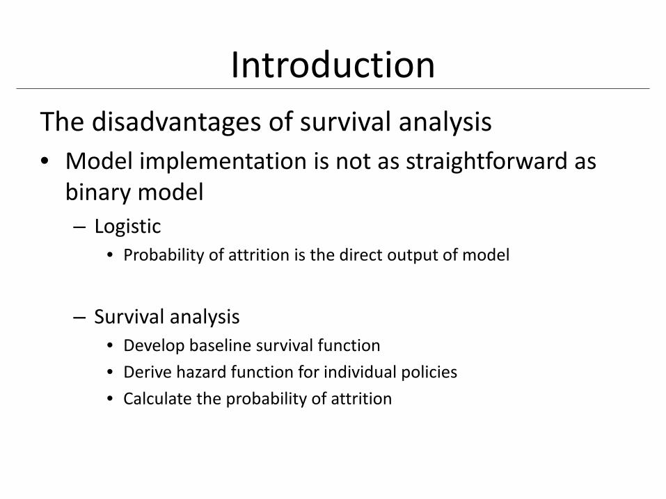
IntroductionThe disadvantages of survival analysis• Model implementation is not as straightforward as
binary model– Logistic
• Probability of attrition is the direct output of model
– Survival analysis• Develop baseline survival function• Derive hazard function for individual policies• Calculate the probability of attrition

IntroductionThe disadvantages of survival analysis• Time-varying macroeconomic variables are more
difficult to predict than retention– How to capitalize the relationship between retention and
time-varying macroeconomic variables– The models on interest rates and stock indexes are much
more complex then retention models– Macroeconomic variables are more volatile than retention,
and may introduce additional volatility into retention projection.

IntroductionLiteratures on Marketing and Banking• Helsen K. and D. C. Schmittlein, "Analyzing Duration Times in Marketing: Evidence for the
Effectiveness of Hazard Rate Models", Marketing Science, 1993, Vol. 12, No. 4, 395-414.• Stepanova M. and L. C. Thomas, "Survival Analysis for Personal Loan Data", Operations
Research, 2002, Vol. 50, 277-289.• Van den Poel D., and B. Lariviere, “Customer Attrition Analysis for Financial Services
using Proportional Hazard Models", European Journal of Operational Research, 2004, vol. 157, No 1, 196-217
• Graves S, D. Kletter, W. B. Hetzel, R. N. Bolton, “A Dynamic Model of the Duration of the Customer’s Relationship with a Continuous Service Provider: The Role of Satisfaction”, Marketing Science, 1998, Vol. 17, No. 1, pp. 45-65.
• Andreeva G., “European Generic Scoring Models Using Survival Analysis”, Journal of the Operational Research Society, 2006, Vol. 57, No. 10, pp. 1180-1187.
• Bellotti T. and J. Crook, “Credit Scoring With Macroeconomic Variables Using Survival Analysis”, Journal of the Operational Research Society, 2009, Vol. 60, pp. 1699–1707.
• Tang L, L. C. Thomas, S. Thomas, J. F. Bozzetto, "It's the Economy Stupid: Modeling Financial Product Purchases", International Journal of Bank Marketing, 2007, Vol.25, No 1, 22-38.

Survival Analysis• Another name for time to event analysis • Statistical methods for analyzing survival
data.• Primarily developed in the medical and
biological sciences (death or failure time analysis)
• Widely used in the social and economic sciences, as well as in Insurance (longevity, time to claim analysis).

Survival AnalysisSurvival Time • t measures the time from a particular
starting time (e.g., time initiated the treatment) to a particular endpoint of interest (e.g., patient died).
• Examples: – Insurance Policy: Started at Jan2008, terminated
at Aug2012. – Products: Bought at Dec2006, failed at Feb2009. – Marketing: coupon mailed at Jan2013,
redeemed at March 2013.

Survival Analysis
Censoring • Occurs when the value of a measurement or
observation is only partially known. • Left Censoring:
Example: Subject's lifetime is known to be less than a certain duration.
• Right Censoring: Example: Subjects still active when they are lost to follow-up or when the study ends.

Survival Analysis
Data• Calendar time of whole study (Starting day,
Ending day of the whole study period) • Study Duration of each individual. • Define the censored observations.• Time measure units (Month, Year … )• Define the dependent variable and independent.

Survival Analysis

Cox Proportional Hazard Model
Advantages• The dependent variable of interest
(survival/failure time) is most likely not normally distributed.
• Censoring(especially right censoring) of the Data.
• Baseline hazard function is unknown.• Whether and when the customer will leave.• Dynamics covariates and duration

Cox Proportional Hazard Model
Hazard equations: hazard rate at time t for an individual have
covariate value,
Here
k is the total number of the covariates, is the constant Proportional effect of
The term h0(t) is called the baseline hazard; it is the hazard for the respective individual when there is no covariate impacts.
),,,( 21 ktttt xxxx =
tx
),,,( 21 kββββ =
jβ
jx
txt ethxth
'
)()|( 0β=
)|( txth
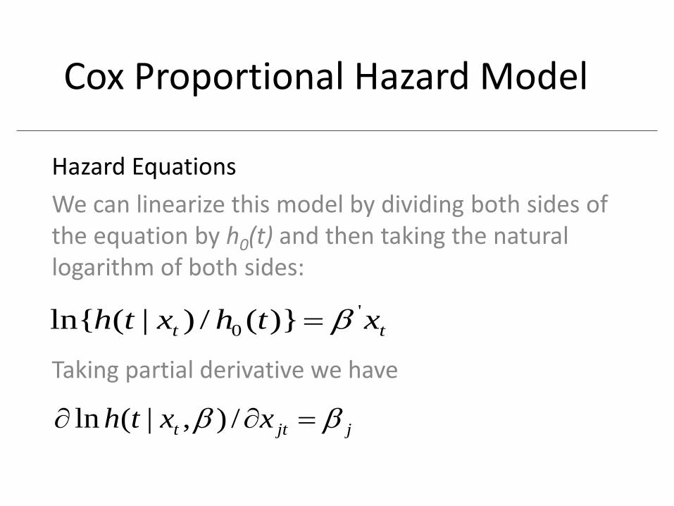
Cox Proportional Hazard Model
Hazard EquationsWe can linearize this model by dividing both sides of the equation by h0(t) and then taking the natural logarithm of both sides:
Taking partial derivative we have
tt xthxth '0 )}(/)|(ln{ β=
jjtt xxth ββ =∂∂ /),|(ln

Literatures on Survival Analysis Theory• Cox, D. R., "Regression Models and Life Tables (with discussion),"
Journal of the Royal Statistical Society Series B, 1972, Vol. 34, 187-220.
• Efron, B., “Logistic Regression, Survival Analysis, and the Kaplan-Meier Curve”, Journal of American Statistical Association, 1988, Vol. 83, 414-425.
• Flinn, C. and J. Heckman, "New Methods for Analyzing Structural Models of Labor Force Dynamics", Journal of Econometrics, 1982, vol. 18(1), 115-168.
• Kaplan, E.L. & Meier, P. "Nonparametric Estimation from Incomplete Observations," Journal of the American Statistical Association, 1958, Vol 53, 457-481.
Cox Proportional Hazard Model

Case StudyData• Simulated commercial line data. • Dependent variable:
Duration = the time until the policy leaves • If a policy is still effective at the end of study, it is
right censored ( i.e. Censor = 1) • External data (including macroeconomic data) are
joined into policy data.

Case StudyData• Define rate changes, removing the impacts from
― Exposure changes (add a building; cut a class)― Coverage changes (reduce limits; increase deductible) ― Risk characteristics changes (have a violation/claim;
add a youthful driver)• Groupings/binnings can be arbitrary
― Contractors vs. noncontractors― Size groups― Variable interactions:
― Small, medium, large contractors― General, nongeneral with sub, artisan contractors

Annual Attrition Summary
* The data is for illustration purpose.
Year Total RenewedNon
Renewed Midterm
CancellationNon
Renewal % Midterm
Cancellation % Retention %
1 197,954 156,477 24,570 16,907 12.41% 8.54% 79.05%
5 211,061 162,875 27,398 20,788 12.98% 9.85% 77.17%
Case Study

Case Study
6.00%
7.00%
8.00%
9.00%
10.00%
11.00%
12.00%
13.00%
14.00%
1 2 3 4 5Year
Annual attrition: end-term vs. mid-term
End-term
Mid-term
Annual Attrition Summary

Annual Attritions by Policy Age
Case Study
4.0%
6.0%
8.0%
10.0%
12.0%
14.0%
16.0%
18.0%
20.0%
1 2 3 4 5Year
Annual Attrition: NB vs old policies
NB end term
Old end term
NB mid term
Old mid term

Annual Attritions by Policy Category
Case Study
4.0%
6.0%
8.0%
10.0%
12.0%
14.0%
16.0%
1 2 3 4 5Year
Annual Attrition: monoline vs package
Mono end term
Package end term
Mono mid term
Package mid term

Case StudyMonthly View: March Year1
Active Attrition PercentEnd-term 16,939 2,086 12.32%
Others 182,160 1,609 0.88%Total 199,099 3,695 1.86%
10.0%
10.5%
11.0%
11.5%
12.0%
12.5%
13.0%
13.5%
14.0%
Year
1Mar
Year
1Jun
Year
1Sep
Year
1Dec
Year
2Mar
Year
2Jun
Year
2Sep
Year
2Dec
Year
3Mar
Year
3Jun
Year
3Sep
Year
3Dec
Year
4Mar
Year
4Jun
Year
4Sep
Year
4Dec
Year
5Mar
Year
5Jun
Year
5Sep
Year
5Dec
Monthyl View: End-term Nonrenewal Rate
0.6%
0.7%
0.8%
0.9%
1.0%
1.1%
1.2%
1.3%
1.4%
Year
1Mar
Year
1Jun
Year
1Sep
Year
1Dec
Year
2Mar
Year
2Jun
Year
2Sep
Year
2Dec
Year
3Mar
Year
3Jun
Year
3Sep
Year
3Dec
Year
4Mar
Year
4Jun
Year
4Sep
Year
4Dec
Year
5Mar
Year
5Jun
Year
5Sep
Year
5Dec
Monthly View: Mid-term Cancellation Rate

Monthly Attritions by Policy Size
Case Study
0.0%
5.0%
10.0%
15.0%
20.0%
25.0%
30.0%
35.0%
Year1Sep Year2Sep Year3Sep Year4Sep Year5SepMonth
Monthly end-term attrition: by policy size
Small
Mid
Large
0.0%
0.2%
0.4%
0.6%
0.8%
1.0%
1.2%
1.4%
Year1Sep Year2Sep Year3Sep Year4Sep Year5SepMonth
Monthly mid-term attrition: by policy size
Small
Mid
Large

Monthly Attritions: Contractors vs. noncontractors
Case Study
4.0%
6.0%
8.0%
10.0%
12.0%
14.0%
16.0%
18.0%
Year1Sep Year2Sep Year3Sep Year4Sep Year5SepMonth
End-term attrition: contractors vs other
Contractor
Other
0.4%
0.5%
0.6%
0.7%
0.8%
0.9%
1.0%
1.1%
1.2%
1.3%
Year1Sep Year2Sep Year3Sep Year4Sep Year5SepMonth
Mid-term attrition: contractors vs other
Contractor
Other
Case Study
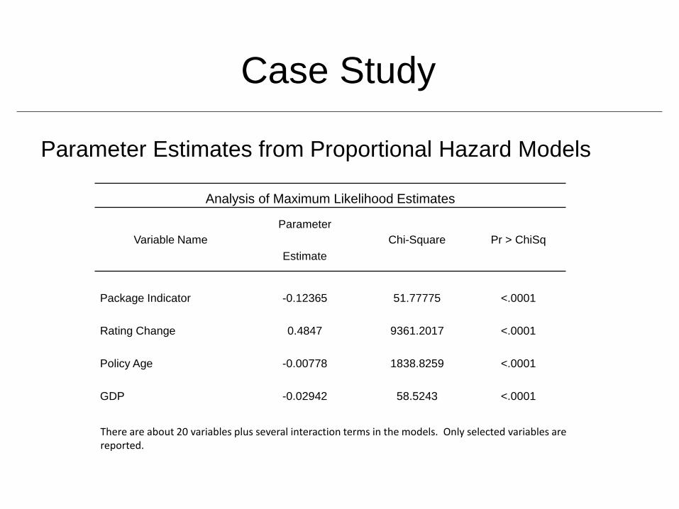
There are about 20 variables plus several interaction terms in the models. Only selected variables are reported.
Analysis of Maximum Likelihood Estimates
Variable NameParameter
Chi-Square Pr > ChiSqEstimate
Package Indicator -0.12365 51.77775 <.0001
Rating Change 0.4847 9361.2017 <.0001
Policy Age -0.00778 1838.8259 <.0001
GDP -0.02942 58.5243 <.0001
Parameter Estimates from Proportional Hazard Models

Parameter Estimates from Logistic Regression
Logit Analysis of Maximum Likelihood Estimates
Variable NameParameter
Chi-Square Pr > ChiSqEstimate
Package Indicator -0.1542 63.52335 <.0001
Rating Change 0.4167 899.4738 <.0001
Policy Age -0.00691 3590.2861 <.0001
GDP -0.0245 16.4331 <.0001
Case Study

Survival Curve for Policy Age
Case Study

Survival Curve for Policy Category
Case Study

Survival Curve for GDP Change (Percent)
Case Study

Survival Curve for Market Condition
Case Study

Validation of the Models (Table)
ModelDecile
AvailableObs
AttritionObs
AttritionRate
CumulativeQuantity
1 9,625 3,697 38.41% 9,625
2 9,627 2,714 28.19% 19,252
3 9,624 2,356 24.48% 28,876
4 9,628 2,116 21.98% 38,504
5 9,628 1,935 20.10% 48,132
6 9,626 1,722 17.89% 57,758
7 9,627 1,677 17.42% 67,385
8 9,625 1,498 15.56% 77,010
9 9,628 1,245 12.93% 86,638
10 9,626 1,054 10.95% 96,264
Total 96,264 20,014 20.79% 96,264
ModelDecile
AvailableObs
AttritionObs
AttritionRate
CumulativeQuantity
1 9,622 3,567 37.07% 9,622
2 9,630 2,790 28.97% 19,252
3 9,627 2,303 23.92% 28,879
4 9,626 2,148 22.31% 38,505
5 9,628 1,929 20.04% 48,133
6 9,626 1,758 18.26% 57,759
7 9,626 1,641 17.05% 67,385
8 9,626 1,450 15.06% 77,011
9 9,627 1,310 13.61% 86,638
10 9,626 1,118 11.61% 96,264
Total 96,264 20,014 20.79% 96,264
Out-of-sample Performance of Survival Analysison the 1 year attrition
Out-of-sample Performance of Logistic Regressionon the 1 year attrition
Case Study
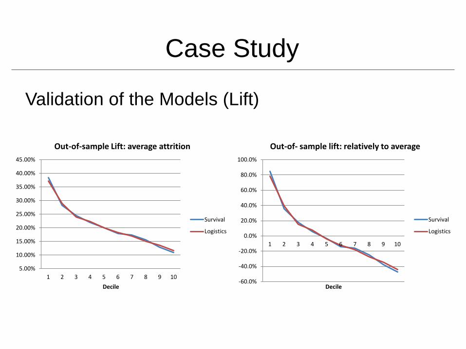
Validation of the Models (Lift)
Case Study
5.00%
10.00%
15.00%
20.00%
25.00%
30.00%
35.00%
40.00%
45.00%
1 2 3 4 5 6 7 8 9 10Decile
Out-of-sample Lift: average attrition
Survival
Logistics
-60.0%
-40.0%
-20.0%
0.0%
20.0%
40.0%
60.0%
80.0%
100.0%
1 2 3 4 5 6 7 8 9 10
Decile
Out-of- sample lift: relatively to average
Survival
Logistics

Validation of the Models (Gini Chart)
Out –of-sample Performance of Survival Analysison the 1 year attrition
Out –of-sample Performance of Logistic Regressionon the 1 year attrition
Case Study

Conclusions• Survival analysis addresses not only whether a policy will
leave, but also when it will leave.• Provide a dynamic insight by utilizing panel data and
improve the static view derived from snapshot data.• Analyze mid-term cancellation and end-term nonrenewal
sequentially and simultaneously.• Able to measure the impacts of time-variant
macroeconomic variables on attrition.• Empirical study does not show significant lift improvement
over logistics regression