1

Establishing correction solutions for Scanning Laser Doppler

Vibrometer measurements affected by sensor head vibration

Ben J. Halkon1 and Steve J. Rothberg2

1Centre for Audio, Acoustics & Vibration, Faculty of Engineering & IT,

University of Technology Sydney, Ultimo, NSW 2007, Australia

2Wolfson School of Mechanical, Electrical and Manufacturing Engineering,

Loughborough University, Loughborough, Leicestershire, LE11 3TU, UK.

Corresponding author: Ben Halkon

e-mail: Benjamin.Halkon@uts.edu.au,

tel: +61 (0) 2 9514 9442

2

Establishing correction solutions for Scanning Laser Doppler

Vibrometer measurements affected by sensor head vibration

Ben J. Halkon1 and Steve J. Rothberg2

1Centre for Audio, Acoustics & Vibration, Faculty of Engineering & IT,

University of Technology Sydney, Ultimo, NSW 2007, Australia

2Wolfson School of Mechanical, Electrical and Manufacturing Engineering,

Loughborough University, Loughborough, Leicestershire, LE11 3TU, UK.

Abstract

Scanning Laser Doppler Vibrometer (SLDV) measurements are affected by sensor head vibrations as

if they are vibrations of the target surface itself. This paper presents practical correction schemes to

solve this important problem. The study begins with a theoretical analysis, for arbitrary vibration and

any scanning configuration, which shows that the only measurement required is of the vibration

velocity at the incident point on the final steering mirror in the direction of the outgoing laser beam

and this underpins the two correction options investigated. Correction sensor location is critical; the

first scheme uses an accelerometer pair located on the SLDV front panel, either side of the emitted

laser beam, while the second uses a single accelerometer located along the optical axis behind the

final steering mirror.

Initial experiments with a vibrating sensor head and stationary target confirmed the sensitivity to

sensor head vibration together with the effectiveness of the correction schemes which reduced overall

error by 17 dB (accelerometer pair) and 27 dB (single accelerometer). In extensive further tests with

both sensor head and target vibration, conducted across a range of scan angles, the correction schemes

reduced error by typically 14 dB (accelerometer pair) and 20 dB (single accelerometer). RMS phase

error was also up to 30% lower for the single accelerometer option, confirming it as the preferred

option. The theory suggests a geometrical weighting of the correction measurements and this provides

a small additional improvement.

Since the direction of the outgoing laser beam and its incident point on the final steering mirror both

change as the mirrors scan the laser beam, the use of fixed axis correction transducers mounted in

fixed locations makes the correction imperfect. The associated errors are estimated and expected to be

generally small, and the theoretical basis for an enhanced three-axis correction is presented.

KEYWORDS: Scanning Laser Doppler Vibrometer; vibration measurement; instrument vibration;

measurement error correction.

3

1 Introduction

The Scanning Laser Doppler Vibrometer (SLDV) has become widely deployed in many application

domains as a convenient, reliable and accurate whole-field vibration measurement system [1]. Myriad

applications have been conceived, researched, developed and largely perfected with many now readily

accepted alongside those using more conventional sensors such as accelerometers or strain gauges.

Indeed, in many cases, SLDV-based measurement campaigns offer significantly enhanced insights

due to their inherent non-invasiveness, measurement of the optimum vibration parameter (velocity),

higher spatial resolution, and wider frequency and dynamic ranges, with further practical benefits

from remote operation and speed of set-up.

This paper addresses one of the remaining challenges to overcome, which is the sensitivity of the

measurement to the SLDV’s own vibration because LDVs, whether scanning or fixed beam, make a

relative vibration velocity measurement. Vibration of the LDV body or of any beam steering optical

elements, either within or external to the instrument, introduce additional Doppler shifts to the laser

beam which add erroneously to the measured velocity and are indistinguishable from the desired

measurement of target surface velocity. In some applications, these erroneous contributions might be

low level or in a frequency range that allows them to be differentiated from the intended measurement

and disregarded. For example, tripod mounting of the instrument, which is routine with SLDV, might

ensure instrument vibrations are confined to a low frequency range below that of interest for target

vibration. In general, however, correction is the only reliable method of eliminating these erroneous

velocity components and this paper sets out the theoretical basis and practical implementation of

schemes to solve this problem.

Employing common principles, earlier studies have demonstrated measurement correction for

instrument vibration [2] and for steering optic vibration [3]. The subject of these studies was the

standard (fixed/single beam) LDV, with a comprehensive mathematical approach used to determine

the total velocity measured for arbitrary target and instrument/steering optic vibrations. The output

from this totally general, vector-based method provided the theoretical basis for the practical

compensation scheme which has been shown experimentally to offer (near) complete correction of the

measured velocity for typical real-world vibration levels [2]-[4]. Recent similar campaigns have been

reported, some making use of and extending these recommendations [5], and others employing

alternative approaches with some success [6].

This comprehensive study builds on these earlier studies and includes a confirmation of the

measurement sensitivity to sensor head vibration, the theoretical basis of the proposed correction

schemes for arbitrary instrument vibration, and real-world relevant laboratory tests to confirm their

effectiveness. To the authors’ knowledge, this is the first published presentation of practical schemes

to correct errors associated with vibrations of the sensor head for Scanning LDVs.

4

2 Theoretical basis for the correction of SLDV sensor head vibration

2.1 General considerations

It has been shown in a variety of circumstances [2], [3], [7] how the Doppler shifts associated with the

vibrations of the instrument itself and of beam steering devices contribute additively to the

measurement being made. Consequently, in a system such as the Scanning LDV with multiple beam

steering devices, compensations for each of these additive Doppler shifts can also be summed to

correct measurements. Summing compensations in this way, however, represents a significant

measurement burden from both cost and practicality perspectives. The SLDV head used in this work,

shown schematically in Figure 1, would require one or two accelerometers mounted on the LDV body

[2], [4] and at least one accelerometer mounted on each of the steering mirrors [3]. The burden is

compounded by the problem of mounting a contacting transducer on a scanning mirror which would

severely challenge the stability of the mirror galvanometer dynamics. The LDV body and the

scanning mirrors move together as a rigid body, however, and this paper will show theoretically and

confirm experimentally how this enables a much more practical solution to the vibration

compensation challenge.

[INSERT: Figure 1. Experimental arrangement schematic showing laser beam path and local

coordinate system.]

The test SLDV used the same pair of scanning mirrors, associated electronics and optical layout as the

Polytec Scanning Vibrometer PSV 300 [8] but instead incorporated a Polytec Compact Laser

Vibrometer NLV-2500-5 [9] as the measurement LDV sensor head. The custom system affords good

access to the preferred correction measurement locations, as can be seen in Figure 2 which shows

several views of the internal optical arrangement corresponding to Figure 1. However, it is important

to emphasise that the proposed measurement correction scheme is sufficiently simple and practical

that it can be readily implemented in any system, commercial or otherwise.

[INSERT: Figure 2. Experimental arrangement physical set-up; a) LDV body mounted to bespoke

SLDV assembly, b) top view with SLDV cover removed showing ‘AccR’, ‘AccFL’ and ‘AccFR’, and

‘AccTar’ with laser beam path super-imposed, c) side view showing SLDV assembly front panel with

‘AccFL’ & ‘AccFR’ and shaker with laser beam path super-imposed and d) close-up of vibrating

target with ‘AccTar’.]

2.2 Mathematical determination of the required correction

Figure 1 shows the instrument configuration in use with each beam orientation described by unit

vectors. Following the path of the laser beam from the LDV sensor head, the first steering mirror is

fixed, while the second and third mirrors are able to rotate to reorient, or scan, the laser beam. The

5

laser beam exits the LDV body with direction unit vector 𝑏"# and passes through reference point O.

The beam is then deflected from the fixed steering mirror at point A on the mirror surface, changing

its direction to 𝑏"$. Reflection from (fixed) point B on the ‘y-scan’ steering mirror changes the beam

orientation to 𝑏"% and then reflection from (variable) point C on the ‘x-scan’ steering mirror redirects

the beam to its final orientation, 𝑏"&.

Following the vector-based approach [7], the total measured velocity, 𝑈(, can be written as the sum

of the velocities associated with the Doppler shifts resulting from LDV body vibration [2], the

direction change at each mirror surface [3] and the desired measurement, )𝑏"&. 𝑉,-..... 0, of target vibration:

𝑈( = 𝑏"#. 𝑉2.... + )𝑏"$ − 𝑏"#0. 𝑉5.... + )𝑏"% − 𝑏"$0. 𝑉6.... + )𝑏"& − 𝑏"%0. 𝑉7.... − 𝑏"&. 𝑉,-..... (1)

With point O as the arbitrarily chosen reference point, the velocity vectors at each of the points A, B

and C, described by position vectors 𝑟5... , 𝑟6... and 𝑟7... , can be written as follows:

𝑉5.... = 𝑉2.... + 𝑟5... × 𝜔.. (2a)

𝑉6.... = 𝑉2.... + 𝑟6... × 𝜔.. (2b)

𝑉7.... = 𝑉2.... + 𝑟7... × 𝜔.. (2c)

where 𝜔.. is the arbitrary angular velocity around the reference point. Equations (2a-c) make explicit

the special relationship between the velocities at the incident points on the steering mirrors which are

united by the reference velocity 𝑉2.... and the angular velocity 𝜔.. under the reasonable assumption

(based on consideration of the frequency range in which instrument vibration is likely in practice) that

the SLDV instrument responds to ambient vibration as a rigid body.

Equation (1) can be reorganised to show the influence of the individual beam orientations:

𝑈( = 𝑏"#. )𝑉2.... − 𝑉5.... 0 + 𝑏"$. )𝑉5.... − 𝑉6.... 0 + 𝑏"%. )𝑉6.... − 𝑉7.... 0 + 𝑏"&. )𝑉7.... − 𝑉,-..... 0 (3a)

and then re-written by substituting in equations (2a-c):

𝑈( = −𝑏"#. (𝑟5... × 𝜔.. ) + 𝑏"$. )(𝑟5... − 𝑟6... ) × 𝜔.. 0 + 𝑏"%. )(𝑟6... − 𝑟7... ) × 𝜔.. 0 + 𝑏"&. )𝑉7.... − 𝑉,-..... 0 (3b)

In the first triple scalar product, vectors 𝑏"# and 𝑟5... are by definition parallel so the triple scalar product,

which can be re-ordered as 𝜔.. . )𝑏"# × 𝑟5... 0, evaluates to zero. For the second and third triple scalar

products, note how the vector differences (𝑟5... − 𝑟6... ) and (𝑟6... − 𝑟7... ) are each equal to vectors with

direction equal to the associated laser beam orientations, 𝑏"$ and 𝑏"% respectively. These triple scalar

products also, therefore, evaluate to zero for the same reason as the first one. Consequently, the

measured velocity is simply:

𝑈( = 𝑏"&. )𝑉7.... − 𝑉,-..... 0 (3c)

6

Equation (3c) represents the first significant outcome in this paper, for several reasons as follows. At

the most general level, the analysis made no restrictive assumptions about the instrument vibration or

the steering mirror orientations, all were entirely arbitrary. The analysis can also be generalised to any

number of beam deflections since each will simply add another triple scalar product to equation (3b)

that will evaluate to zero in the manner described above. Consequently, equation (3c) holds for

arbitrary vibration of any SLDV head, provided the assumption of rigid body motion of LDV body

and mirrors holds. Ultimately and most importantly because of the practical implication, it means that

the compensation requires only a measurement of )𝑏"&. 𝑉7.... 0 followed by subtraction from 𝑈( and so, at

the very least, the correction measurement burden has been significantly reduced from multiple

measurements on the LDV body and at each steering mirror to measurement of a single velocity

component.

2.3 Practical determination of the required correction

However, while the measurement required for compensation might look much simpler now, it is not

entirely straightforward to achieve practically. Firstly, the point C varies according to the orientation

of any beam steering optics that precede this final steering mirror. In the setup used here [8], a beam

deflection of 12 degrees by the first (y-scan) mirror causes the beam to move about 7 mm along the

axis of the final (x-scan) mirror. Secondly, if a transducer is to be fixed to the mirror, as in previous

steering mirror vibration compensation work [3], this time the required orientation is in the direction

of the outgoing laser beam and not in the more convenient (from the perspective of mounting an

accelerometer on the back of the mirror) mirror normal direction. Finally, the difficulty here is

compounded by the beam orientation being necessarily variable in Scanning LDV.

The practical locations at which to locate transducers for compensating measurements follow the

principles adopted in previous work [2]-[4]. In those applications, only a single axis measurement was

required for theoretically perfect compensation. The essential principle is that the compensating

measurement must be co-linear with the laser beam itself. The same principle applies in the SLDV

application but the practicality associated with maintaining a measurement that is aligned with a

scanning laser beam is problematic. This paper will first explore quantitively the viability of

compensation with measurements that are perfect only when the beam is in its ‘zero’ position. This

analysis is then developed to a more comprehensive proposal where all three components of vibration

are measured for full compensation.

Practically, compensation options are limited to measurements at locations remote from C and in

fixed directions. Following earlier successful approaches, the options available are location of a pair

of transducers on the front face of the instrument equi-spaced either side of the line of the undeflected

laser beam [2] or location of a single transducer in line with the undeflected laser beam [4] but at the

7

rear of the final scanning mirror fixed to some convenient part of the mirror housing (not the mirror

itself).

With the scanning mirrors in their ‘zero’ positions and the LDV optical axis perfectly aligned with

that of the scanning system, the laser beam will be incident on the mirror at point C0, defined by a

position vector 𝑟7C..... . The velocity at this point, 𝑉7C...... , is:

𝑉7C...... = 𝑉C... + 𝑟7C..... × 𝜔.. (4)

For compensating measurements using the accelerometer pair on the front face of the instrument (left

and right, shown as ‘AccFL’ and ‘AccFR’ in Figure 1), the position vectors, 𝑟DE..... and 𝑟DF...... , are:

𝑟DE..... = 𝑟7C..... + 𝑟7C/DH𝑥JEKL + 𝑟7C/DM𝑦JEKL + 𝑟7C/DO��EKL (5a)

𝑟DF...... = 𝑟7C..... − 𝑟7C/DH𝑥JEKL − 𝑟7C/DM𝑦JEKL + 𝑟7C/DO��EKL (5b)

where 𝑟7C/DH, 𝑟7C/DM, and 𝑟7C/DO are the three components of the transducer locations in a coordinate

system fixed in the SLDV. The ��EKL direction is the instrument’s primary sensitive direction and

follows the line of the returning laser beam in its zero position. The orthogonal directions are also

related to beam orientation: 𝑦JEKL = 𝑏"$ (always) and 𝑥JEKL = 𝑏"% when the ‘y-scan’ mirror is in its zero

position.

For a single compensating measurement at the rear of the second scanning mirror (shown as ‘AccR’

in Figure 1), the position vector, 𝑟F... , is:

𝑟F... = 𝑟7C..... + 𝑟7C/FO��EKL (5c)

where 𝑟7C/FO is the z-component of the transducer location in the SLDV coordinate system. The other

components of the position vector are both zero in this case. The vibration velocities, 𝑉DE...... , 𝑉DF...... and

𝑉F.... ,at these locations can be written as:

𝑉DE...... = 𝑉C... + )𝑟7C..... + 𝑟7C/DH𝑥JEKL + 𝑟7C/DM𝑦JEKL + 𝑟7C/DO��EKL0 × 𝜔.. (6a)

𝑉DF...... = 𝑉C... + )𝑟7C..... − 𝑟7C/DH𝑥JEKL − 𝑟7C/DM𝑦JEKL + 𝑟7C/DO��EKL0 × 𝜔.. (6b)

𝑉F.... = 𝑉C... + )𝑟7C..... + 𝑟7C/FO��EKL0 × 𝜔.. (6c)

With the front face accelerometer pair oriented to measure vibration in the ��EKL direction, the

measured velocities, 𝑈DE and 𝑈DF, can be written:

𝑈DE = )��EKL. 𝑉DE...... 0 = ��EKL. )𝑉C... + )𝑟7C..... + 𝑟7C/DH𝑥JEKL + 𝑟7C/DM𝑦JEKL + 𝑟7C/DO��EKL0 × 𝜔.. 0 (7a)

𝑈DF = )��EKL. 𝑉DF...... 0 = ��EKL. )𝑉C... + )𝑟7C..... − 𝑟7C/DH𝑥JEKL − 𝑟7C/DM𝑦JEKL + 𝑟7C/DO��EKL0 × 𝜔.. 0 (7b)

8

Taking the mean of these measured velocities, as required, and making use of equation (4) to obtain

the correction velocity 𝑈D:

𝑈D =#$(𝑈DE + 𝑈DF) = )��EKL. 𝑉7C...... 0 +

#$��EKL. S)𝑟7C/DH𝑥JEKL + 𝑟7C/DM𝑦JEKL + 𝑟7C/DO��EKL0 × 𝜔.. T +

#$��EKL. S)−𝑟7C/DH𝑥JEKL − 𝑟7C/DM𝑦JEKL + 𝑟7C/DO��EKL0 × 𝜔.. T (8a)

Re-ordering the triple scalar products shows more readily that together they evaluate to zero because

the 𝑥JEKL and 𝑦JEKL components sum to zero leaving only a cross-product between ��EKL and itself:

𝜔.. . S��EKL × )𝑟7C/DH𝑥JEKL + 𝑟7C/DM𝑦JEKL + 𝑟7C/DO��EKL0 + ��EKL × )−𝑟7C/DH𝑥JEKL − 𝑟7C/DM𝑦JEKL +

𝑟7C/DO��EKL0T = 0 (8b)

Consequently:

𝑈D = )��EKL. 𝑉7C...... 0 (8c)

which is equal to the required correction of )𝑏"&. 𝑉7.... 0 when the laser beam is in its zero position.

Following the equivalent analysis for the rear accelerometer, the alternative correction velocity, 𝑈F,

can be written:

𝑈F = )��EKL. 𝑉F.... 0 = ��EKL. )𝑉C... + )𝑟7C..... + 𝑟7C/FO��EKL0 × 𝜔.. 0 (9a)

With the equivalent rearrangement, the measured velocity for this option is also shown to be equal to

the required correction of )𝑏"&. 𝑉7.... 0 when the laser beam is in its zero position:

𝑈F = )��EKL. 𝑉7C...... 0 + ��EKL. S)𝑟7C/FO��EKL0 × 𝜔.. T = )��EKL. 𝑉7C...... 0 (9b)

Either correction velocity, 𝑈D or 𝑈F, is then subtracted from the original SLDV measurement, 𝑈(.

Correction based on either option will be explored experimentally in the following section.

3 Experimental confirmation of measurement correction schemes

3.1 Experimental arrangement

The entire SLDV unit was mounted on a linear bearing, enabling vibration in the z direction (only).

This vibration is generated via an electrodynamic shaker connected to the SLDV body by a stiff

pushrod, as shown in Figure 2c. With the shaker inactive, the SLDV is (nominally) stationary. The

target was another electrodynamic shaker, orientated in line with the sensor head optical axis and

instrumented with an Endevco 770F-010-U-120 variable capacitance ‘DC response’ accelerometer,

‘AccTar’, as shown in Figure 2d. Again, the target is (nominally) stationary when the shaker is not

9

active. The LDV stand-off distance (505 mm) was set to coincide with one of the recommended

working distances for the NLV-2500-5 [9], which takes into account the laser beam path within the

scanning head as well as the distance to the target.

The shakers are driven independently, via appropriate power amplifiers (not shown), with signals

generated within the 8 input/4 output channel configuration B&K LAN-XI/Pulse LabShop data

acquisition system (also not shown).

3.2 Accelerometer sensitivity relative calibration and time delay compensation

Following the procedure established in previous studies [2]-[4] and for optimal measurement

compensation, it is good practice to confirm the accelerometer sensitivities with respect to that of the

LDV but it is essential to measure the finite time delays between the accelerometer channels and that

of the LDV. As shown in Figure 3a, this was practically achieved by mounting the entire

accelerometer set directly onto an electrodynamic shaker. In this image, five similar Endevco

transducers are shown, though only four were subsequently used. The interface between each sensor

is a thin layer of synthetic beeswax, stiff enough to ensure identical vibration occurs in all units across

the frequency range used. The LDV, used as the reference vibration measurement, is aligned with the

accelerometers’ sensitive axes with the probe laser beam focused on the top accelerometer in the

stack.

[INSERT: Figure 3. Amplitude calibration check and time delay calculation; a) experimental set-up

with laser beam path super-imposed, b) mean amplitude comparison with LDV signal after

accelerometer sensitivity adjustment and c) phase difference between LDV and example

accelerometer before and after time delay adjustment.]

A broadband random (white) noise signal to 200 Hz was generated to yield an accelerometer stack

vibration level of between 1 and 10 mm/s. This level is deliberately chosen to be consistent with the

level used in a common accelerometer calibrator, e.g. the Brüel & Kjaer Type 4294 [10] (albeit at

single frequency i.e. 10 mm/s RMS at 159.2 Hz) and with the level that corresponds to a “slightly

rough” running machine [11]. It is therefore reasonable to use in these experiments but the exact level

achieved is not critical since the LDV provides the reference sensitivity against which the relative

accelerometer sensitivities are to be determined.

Five sequential complex frequency spectra (200 Hz range, 0.5 Hz resolution, no overlap) were

directly collected for all channels simultaneously. Frequency domain post-processing conveniently

enables integration of the accelerometer signals to velocity for direct comparison with the LDV. RMS

values for the frequency range between 2.5 and 100 Hz were calculated for each measurement

channel and the ratio for each accelerometer with respect to the LDV was used to re-calculate the

accelerometer sensitivities. The resulting small adjustments, on the order of 1.5-2%, are summarised

in Table 1. Figure 3b shows a comparison of velocity spectra after adjustment; the target

10

accelerometer (‘AccTar’) is arbitrarily selected to illustrate this. As expected, the agreement between

the example accelerometer and LDV signals is very strong, indifferentiable to the eye across the entire

selected frequency range.

[INSERT: Table 1. Summary of accelerometer sensitivities and inter-channel time delays with respect

to the LDV.]

The same data are used to calculate the inter-channel time delays. Figure 3c shows the mean phase

differences for the example accelerometer with respect to the LDV both before (dashed curve) and

after (solid curve) time delay compensation. Prior to time delay compensation, there is a small

positive gradient, indicating a finite time delay between the accelerometer and the LDV channel.

After compensation the gradient is eliminated, indicating that the signals have been time-aligned.

Table 1 also presents the time delays for the four accelerometer channels relative to the LDV channel.

These relative delays come from the signal conditioning systems, not the data acquisition system, and

all very similar at around 0.14 ms, which is to be expected as the accelerometers are the same model

and use the same signal conditioning.

3.3 Experimental confirmation of SLDV sensitivity to sensor head vibration and measurement

correction

Confirmation of the SLDV sensitivity to its own vibration is a logical starting point for the

experimental part of this study. The SLDV shaker was driven with broadband random noise to 200

Hz, to generate vibration at around 1 mm/s RMS (level equivalent to that for a “good” running

machine [11]). The target shaker was not active so the target accelerometer only picks up ambient

vibration. The SLDV laser beam was incident on the ‘stationary’ target. Five complex frequency

spectra (200 Hz range, 0.5 Hz resolution, no overlap) were captured for subsequent frequency domain

processing. Figure 4a shows the average amplitude spectra for the SLDV and target accelerometer

measurements. The difference is clear; the true target vibration is genuinely very low but the SLDV

measurement is at a much higher level because of the vibration of the instrument itself. There are

various features in each spectrum, associated with force and response in the normal way, but the

shapes of the spectra are not important here. The important point is the sensitivity in the SLDV

measurement to vibration of the SLDV itself and that the levels are such that compensation for this

vibration is essential to yield a reliable measurement of the target vibration.

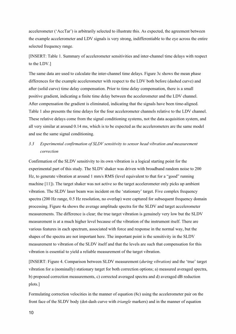
[INSERT: Figure 4. Comparison between SLDV measurement (during vibration) and the ‘true’ target

vibration for a (nominally) stationary target for both correction options; a) measured averaged spectra,

b) proposed correction measurements, c) corrected averaged spectra and d) averaged dB reduction

plots.]

Formulating correction velocities in the manner of equation (8c) using the accelerometer pair on the

front face of the SLDV body (dot-dash curve with triangle markers) and in the manner of equation

11

(9b) using the single accelerometer mounted behind the final scanning mirror (dot-dash curve with

square markers) validates the use of these equations for compensation as well as the hypothesis that

sits behind them. Figure 4b shows excellent agreement between the measurements for both correction

options and the original SLDV measurement. This confirms the SLDV sensitivity to its own vibration,

according to equation (3c), and is the second important finding in this paper.

Notably, however, the agreement is less good between the original SLDV measurement and the

correction derived from the accelerometer pair on the front face of the SLDV body in the frequency

range above approximately 70 Hz. This can be attributed to the dynamic response of the relatively

flexible SLDV body front panel to which the accelerometer pair is fixed. (Indeed, the agreement was

improved by subsequently tightening the screws on the SLDV body i.e. by stiffening the panel). The

requirement for rigid body vibration of the instrument, as explained alongside the presentation of

equations (2a-c), is, to be precise, that the laser, scanning mirrors and compensation measurement

location(s) move as a rigid body and the location of the single accelerometer, which is mounted to a

relatively stiff mirror galvanometer mounting bracket, better fulfils this requirement. This observation

has an important implication for the final choice of correction measurement location.

Notwithstanding this issue, both correction options offer significant improvement to the original

problematic SLDV measurement, as shown in Figure 4c. The correction is of course less good at the

higher frequencies for the accelerometer pair option but, for the single accelerometer mounted on the

stiff bracket behind the final scanning mirror, correction is excellent across the entire frequency range.

An exact match in the figure between the ‘true’ target vibration (from the target accelerometer) and

the corrected SLDV measurement cannot reasonably be expected because the data are essentially a

comparison between two extremely low vibration levels presented on a log scale. (Note that, while the

data presented in Figure 4a-c are averaged over the five individual spectra, the correction is applied at

the individual spectrum level.)

Expressing the improvement as a dB error reduction, based on equation (A5) from Appendix A, is a

standard approach in such circumstances and Figure 4d shows this dB reduction for both the

accelerometer pair (16.8 dB mean) and single accelerometer (26.6 dB mean) options. Such significant

reductions further validate equation (3c) and confirm the effectiveness of equations (8c) and (9b) in

providing the necessary correction velocity.

3.4 Measurement correction for simultaneous SLDV and target vibration

Having demonstrated SLDV measurement sensitivity to vibration of the instrument itself and the

potential for effective correction, the next step is to examine the case of simultaneous target and

instrument vibration. Independent, broadband random target and SLDV vibrations were arranged with

levels in the range 1-2 mm/s RMS. As can be seen in Figure 5a, the differences between the SLDV

measurement and the ‘true’ target vibration are evident, particularly in the frequency range up to 20

12

Hz. Again, there is no special significance to the spectral shape of either measurement. No control has

been exerted over the particular combination of forces and responses as the correction can (and must)

be applied in any circumstances.

[INSERT: Figure 5. For simultaneous target and SLDV sensor head vibration, comparison between

measurements from the SLDV and of the ‘true’ target vibration; a) measured averaged spectra, b)

proposed correction measurements, c) corrected averaged spectrum (single accelerometer only), d)

averaged dB reduction (single accelerometer only) and e) example phase difference spectrum (single

accelerometer only).]

The formulated corrections are shown in Figure 5b for comparison with the original SLDV

measurement. As before, correction has been formulated from the accelerometer pair (dot-dash with

triangle marker) and the single accelerometer (dot-dash with square marker). It is clear from the

comparison between the uncorrected SLDV measurement and the true target vibration that correction

will be significant in the region up to 20 Hz, less significant but still important up to around 50 Hz and

then less important above 50 Hz where the SLDV measurement appears dominated by genuine target

vibration. The flexibility of the front panel plate is again evident in the formulated accelerometer pair

correction around 80-90 Hz.

Applying either of the corrections results in an impressive improvement to the SLDV measurement.

Figure 5c shows this, in the interests of brevity and clarity, for the single accelerometer option only.

Visually, there is excellent agreement between the corrected SLDV measurement and the true target

vibration, across the entire frequency range. The dB error reduction shown in Figure 5d gives more

quantitative insight. Here, the mean reduction over the displayed frequency range is 19.7 dB (15.1 dB

for the accelerometer pair correction, not shown). In the range 2.5-20 Hz, where the need for

significant correction was observed, the error is reduced by 26 dB, while from 20-50 Hz, where more

modest correction was needed, the error is reduced by 22 dB. Above 50 Hz, where the original SLDV

measurement appeared not to need significant correction, the error reduction is small, as expected, but

still around 5 dB. Figure 5e shows, in this case for one of the individual spectra sets, the phase error,

based on equation (A9) from Appendix A, between a corrected SLDV measurement and the true

vibration measurement. Good agreement is observed across the entire frequency range, with

especially good agreement in the frequencies above approximately 20 Hz where there is reasonable

vibration level for both signals. Phase errors are larger at low frequencies where the true vibration

level is low and integration noise (in the conversion of accelerometer measurements to velocity) is

significant.

13

4 Experimental validation of measurement correction during scanning

4.1 Measurement correction during scanning

Demonstrating the correction for sensor head vibration of SLDV measurements is important and has

not previously been reported. However, in the configuration presented so far, with the laser beam in

its zero position, the measurement has been fundamentally the same as that from a fixed beam LDV.

One of the main differentiators of this study is its consideration of the effect of sensor head vibration

on SLDV measurements when the laser beam is oriented away from its zero position i.e. when 𝑏"& ≠

��EKL and when 𝑏"& is variable. Furthermore, it is necessary to find a means of correction that balances

simplicity with effectiveness.

With reference to Figure 1 and Figure 6, the orientation vector 𝑏"& can be expanded (see Appendix B)

in terms of the mirror scan angles, 𝜃M (first, ‘y-scan’ mirror) and 𝜃H (second, ‘x-scan’ mirror), as

follows:

𝑏"& = −cos 2𝜃M sin 2𝜃H 𝑥JEKL + sin 2𝜃M 𝑦JEKL − cos 2𝜃M cos 2𝜃H ��EKL (10)

The required correction can then be written as:

)𝑏"&. 𝑉7.... 0 = −cos 2𝜃M sin 2𝜃H )𝑥JEKL. 𝑉7.... 0 + sin 2𝜃M )𝑦JEKL. 𝑉7.... 0 − cos 2𝜃M cos 2𝜃H )��EKL. 𝑉7.... 0 (11)

Equation (11) shows clearly that full correction requires measurements of 𝑉7.... rather than 𝑉7C...... , of three

components of 𝑉7.... and of mirror scan angles. However, it is also clear that proximity dictates 𝑉7C...... ≈ 𝑉7....

unless there is some reason to expect particularly high levels of angular motion. While, especially for

smaller scan angles, the dominant term in the correction will be the ��EKL component such that:

)𝑏"&. 𝑉7.... 0 ≈ − cos 2𝜃M cos 2𝜃H )��EKL. 𝑉7C...... 0 (12)

Equation (12) indicates that correction also requires a geometrical weighting, cos 2𝜃M cos 2𝜃H, to be

applied to the correction measurement made. However, this weighting is only small. Without it, the

error in the compensation can be written as:

𝑒 = 1 − )��EKL. 𝑉7C...... 0 )𝑏"&. 𝑉7.... 0` = 1 − #abc $de abc $df

(13)

which evaluates to, for example, only 2.2% error for 12° beam deflection for one mirror.

[INSERT: Figure 6. (a) Top, side and front view schematic diagrams showing laser beam path and

correction accelerometer locations. (b) Physical set-up showing mirror rotations, beam path (super-

imposed) and target.]

Consequently, the next set of experiments explore the effectiveness of a single correction

measurement of )��EKL. 𝑉7C...... 0 for the situation where 𝑏"& ≠ ��EKL and this will be undertaken with and

14

without the geometrical weighting indicated by equation (12). The experimental set-up drives SLDV

vibration in the ��EKL direction only (though some inevitable angular motion is also expected) so this

analysis is concentrated on the consequences of measurement of a component of 𝑉7C...... rather than of 𝑉7....

and the importance of the geometrical weighting.

Figure 6 shows positive sense x-scan and y-scan mirror angles that result in positive sense laser beam

deviation in the target plane in the x and y directions. The scanning mirrors are driven by application

of 0.25 V per degree optical to each of the galvanometer drive amplifiers [12]. For the experiment,

fixed voltages were applied independently to the scanning mirror galvanometer amplifiers to achieve

2° increments in the optical scan angle between -4° and +12° on either x- or y-scan mirrors.

Measurements across the full angular ranges were not considered necessary but the -4° and -2°

scenarios were included to confirm the expected symmetry in behaviour. Once the laser beam

orientation had been set, the target was repositioned to maintain an optimum stand-off distance [9]

and then reoriented to ensure that its vibration direction was aligned with the laser beam direction, as

illustrated by the dashed line in Figure 6a and shown photographically for an example x-scan in

Figure 6b.

Data were collected with both target and instrument undergoing broadband vibration of equivalent

levels to those applied previously. The error reductions described below confirm that the proposed

correction schemes are highly effective and this is the third important finding of this study. Example

amplitude spectra for the two extreme scan angles, -4° and +12°, for the y-scan direction case and

using the single accelerometer correction option are shown in Figure 7a&b. The particular corrections

shown do not include the geometrical weighting but, visually, the corrections work well even for the

larger scan angle. (The corresponding scenarios for the x-scan direction case are similar but are not

shown for the sake of brevity.) For the phase error as a function of frequency, Figure 8 shows two

scenarios from the +12° y-scan, though again all data show similar trends. The lowest overall phase

error is found for the single accelerometer correction option with the geometrical weighting, while the

highest overall error is for the accelerometer pair correction option without the geometrical weighting.

Though not large, the differences are visible in Figure 8 which reveals a low frequency region with

larger errors associated with integration noise, a mid-frequency region where errors are low in both

cases and a higher frequency region where the weaker correction option shows larger errors as a

consequence of noise affecting the smaller vibration amplitudes found in this range. The effect of the

SLDV body response in the range 80-90 Hz, encountered throughout this study, is also apparent in the

plot for the accelerometer pair.

[INSERT: Figure 7. Comparison between measurements from the vibrating SLDV and the ‘true’

target vibration during scanning for single accelerometer correction without geometrical weighting; a)

-4° and b) +12°.]

15

[INSERT: Figure 8. Example phase difference plot comparing correction options during scanning.]

4.2 Quantitative evaluation of the correction options

To compare the correction options quantitatively and more effectively, the mean dB error reduction

was calculated according to equation (A5). Appendix A further develops a total RMS phase error

calculated according to equation (A11). The dB error reductions are presented in Tables 2a&b for the

x-scan and y-scan configurations respectively and the total RMS phase errors are similarly presented

in Tables 3a&b. The correction options are presented in descending order of effectiveness. Each

column of each table represents a single measurement (average for five data captures) with five

channels of data: the SLDV, the target accelerometer and the three accelerometers in use for the two

correction options.

[INSERT: Table 2a: dB error reductions in the frequency range 2.5 to 100 Hz; x-scan.]

[INSERT: Table 2b: dB error reductions in the frequency range 2.5 to 100 Hz; y-scan.]

The clearest trend in the dB error reduction data is the greater reduction associated with the single

accelerometer option compared to the accelerometer pair, from at least 4.4 dB up to as much as 10.3

dB. For any particular correction option, there is no clear trend with scan angle. For the options

including geometrical weighting, this might be expected and suggests that the variation observed in

error reduction is affected mainly by sources such as measurement noise or transducer alignments. For

the options not including geometrical weighting, the effect of geometry might be expected to be

apparent at greater scan angles but this trend is not apparent when observing only an individual row of

the tables. However, the trend is reliably apparent (though small) in the comparison between

equivalent correction options at higher scan angles. For example, in Table 2a for the single

accelerometer configuration and the x-scan direction, inclusion of the geometrical weighting adds 0.1

dB, 0.2 dB and 0.4 dB, for scan angles of 8°, 10° and 12° respectively, to the corresponding error

reductions achieved without the geometrical weighting. While for the accelerometer pair, the

geometrical correction adds 0.1 dB, 0.1 dB, 0.2 dB and 0.3 dB, for scan angles of 6°, 8°, 10° and 12°

respectively, to the error reductions achieved without the geometrical weighting. Similar improvement

is evident in Table 2b for the y-scan direction.

Equation (A7b) in Appendix A allows investigation of why the effect of the geometrical correction is

so small. When the geometrical correction is applied, 𝛼 = 1 and the error reduction, 𝑅#, is limited just

by additive noise in the measurements:

𝑅# = −10 log#C klm(n)oooooooo

7m(n)oooooooop (14a)

16

From Tables 2a&b, an indicative calculation can be made with 𝑅# as 20 dB, i.e. klm(n)oooooooo

7m(n)oooooooop = 0.01.

Without the geometrical correction, 𝛼 = 1 cos 2𝜃M cos 2𝜃H⁄ and the error reduction, 𝑅$, can then

written as:

𝑅$ = −10 log#C[(1 − 𝛼)$ + 0.01] (14b)

For a +12° x- or y-scan, 𝑅$ evaluates to 19.8 dB, i.e. the effect of including the geometrical weighting

is to improve the error reduction by 0.2 dB from 19.8 dB to 20 dB, consistent with the values obtained

experimentally. These data and considerations confirm that the geometrical correction is working as

expected and should be applied but its effect is small relative to that of routine measurement errors.

[INSERT: Table 3a: Total RMS phase errors (mrad) in the frequency range 2.5 to 100 Hz; x-scan.]

[INSERT: Table 3b: Total RMS phase errors (mrad) in the frequency range 2.5 to 100 Hz; y-scan.]

Equivalent trends can be seen in the total RMS phase error data shown in Tables 3a&b. The smaller

error associated with the single accelerometer correction option relative to the accelerometer pair

option is also evident in the phase error, with the single accelerometer option offering lower errors by

20 to 100 mrad. For any particular correction option, there is again no clear trend with scan angle but

the benefit of inclusion of the geometrical weighting is apparent in the comparison between

equivalent correction options at higher scan angles. For example, in Table 3a for the single

accelerometer and the x-scan, including the geometrical weighing takes 10, 31 and 65 mrad, for scan

angles of 8°, 10° and 12° respectively, off the RMS error found without the geometrical weighting.

While for the accelerometer pair, including the geometrical weighting takes 9, 26 and 51 mrad, for

scan angles of 8°, 10° and 12° respectively, off the RMS error incurred without the geometrical

weighting. Similar improvement is evident in Table 3b for the y-scan. The data further confirm that

the geometrical weighting should be applied. Though small, its measurable benefit is provided at

minimal additional cost. Demonstrating that the single accelerometer correction with geometrical

weighting provides the best outcome is a further important finding of this study.

4.3 Enhanced three component correction

While it is clear that the dominant correction component will always be that associated with ��EKL-

vibration because 𝑏"& is always closest to ��EKL, equation (11) indicates that, for vibration components

of similar magnitude, the x-correction will be tan 2𝜃H of the z-correction and the y-correction will be

tan 2𝜃M cos 2𝜃H⁄ of the z-correction. For a 12° beam deflection, these are both slightly in excess of

20% so, while the need for an enhanced correction is very dependent on the particular measurement

scenario, these values do suggest that there is merit for a robust correction setup.

17

The approach is not, as might immediately be expected, to use tri-axial transducers for compensation

since a single sensor location (remote from C itself) cannot satisfy the requirements of all three

correction components. For example, an x-measurement at the AccR location would give:

)𝑥JEKL. 𝑉F.... 0 = 𝑥JEKL. )𝑉C... + )𝑟7C..... + 𝑟7C/FO��EKL0 × 𝜔.. 0 = )𝑥JEKL. 𝑉7C...... 0 + 𝜔.. . )𝑥JEKL × 𝑟7C/FO��EKL0 (15)

in which a residual sensitivity to any angular velocity is clear. The correct location, identified in

Figure 6a (Front view) as ‘AccRx’, is a different one, with only a 𝑥JEKL component in its position

relative to C0. Writing this as 𝑟7C/FH𝑥JEKL, this additional single-axis measurement, 𝑈FH, can be

written as:

𝑈FH = )𝑥JEKL. 𝑉FH...... 0 = 𝑥JEKL. )𝑉C... + )𝑟7C..... + 𝑟7C/FH𝑥JEKL0 × 𝜔.. 0

= )𝑥JEKL. 𝑉7C...... 0 + 𝑥JEKL. )𝑟7C/FH𝑥JEKL × 𝜔.. 0 = )𝑥JEKL. 𝑉7C...... 0 (16a)

The equivalent y-correction, 𝑈FM, requires a third single-axis measurement at a location, ‘AccRy’ (see

Figure 6a (Side view)), with a position vector 𝑟7C/FM𝑦JEKL relative to C0:

𝑈FM = 𝑦JEKL. )𝑉C... + )𝑟7C..... + 𝑟7C/FM𝑦JEKL0 × 𝜔.. 0

= )𝑦JEKL. 𝑉7C...... 0 + 𝑦JEKL. )𝑟7C/FM𝑦JEKL × 𝜔.. 0 = )𝑦JEKL. 𝑉7C...... 0 (16b)

Note also that, in Figure 6a (Side view), the location previously identified as AccR becomes ‘AccRz’

to emphasise that correction at this location is only effective for z-vibration and to be consistent with

the labelling adopted for this enhanced correction. The incident points, C0 and C, are also shown on

this view.

Substituting equations (9b) and (16a&b) into equation (11) leads to an improved compensation as

follows:

)𝑏"&. 𝑉7.... 0 ≈ −cos 2𝜃M sin 2𝜃H 𝑈FH + sin 2𝜃M 𝑈FM − cos 2𝜃M cos 2𝜃H 𝑈FO (17)

The practical implementation of this correction will be the subject of further work.

4.4 Error associated with fixed placement of correction accelerometers

The standard and enhanced corrections proposed by equations (11) and (17) still rely on 𝑉7.... ≈ 𝑉7C...... so

the final part of this paper will estimate the typical error associated with this approximation. The

derivation of the position vector for the exact incident point is set out in Appendix C, which shows:

18

𝑟7... = 𝑟7C..... + u𝐵𝐶0........ u tan 2𝜃M 𝑦JEKL (18)

The error associated with measurement at C0 rather than C can be written as:

𝑒 = x"y.Lz..... {x"y.Lz|.......x"y.Lz.....

(19a)

which can then be re-written, by substituting equations (2c), (4) and (18) into equation (19a), as:

𝑒 =u67C........ u }~� $de�... .)x"y×MJ���0

x"y.Lz|....... �u67C........ u }~� $de�... .)x"y×MJ���0 (19b)

The terms within equation (19b) can be expanded, based on equation (10):

)𝑏"&. 𝑉7C...... 0 = −cos 2𝜃M sin 2𝜃H )𝑥JEKL. 𝑉7C...... 0 + sin 2𝜃M )𝑦JEKL. 𝑉7C...... 0 − cos 2𝜃M cos 2𝜃H )��EKL. 𝑉7C...... 0 (20a)

)𝑏"& × 𝑦JEKL0 = −cos 2𝜃M sin 2𝜃H ��EKL + cos 2𝜃M cos 2𝜃H 𝑥JEKL (20b)

The angular vibration velocity can also be expanded into components, 𝜔H, 𝜔M and 𝜔O, as follows:

𝜔.. = )𝜔H𝑥JEKL + 𝜔M𝑦JEKL + 𝜔O��EKL0 (20c)

such that:

u𝐵𝐶0........ u tan 2𝜃M 𝜔.. . )𝑏"& × 𝑦JEKL0 = u𝐵𝐶0........ u tan 2𝜃M )cos 2𝜃M cos 2𝜃H 𝜔H − cos 2𝜃M sin 2𝜃H 𝜔O0 (20d)

Substituting equations (20a) and (20d) into equation (19b) allows a full analysis of the likely error for

any given scenario but a typical error can be estimated through small angle approximations, with

additional recognition that )��EKL. 𝑉7C...... 0 ≫ u𝐵𝐶0........ u2𝜃M𝜔H for typical values, to yield:

𝑒 ≈u67C........ u$de�f{)O���.Lz|....... 0 (21)

Equation (19b) shows that if the SLDV angular vibration velocity is zero then the associated

measurement error is zero and this is, of course, confirmed in the approximate expression of equation

(21). Similarly, the importance of minimising u𝐵𝐶0........ u to minimise the correction error is clear in

equation (19b) and confirmed in equation (21). In this experimental set-up, i.e. with u𝐵𝐶0........ u of 33.81

mm [8] and a scan angle of 12° (optical), vibration amplitudes of 1 mm/s for the ��EKL component of

𝑉7C...... and of 1 mrad/s for 𝜔H were apparent. If these vibrations were in phase (for the sake of this

indicative calculation), the measurement error associated with measurement of )��EKL. 𝑉7C...... 0 rather than

of )��EKL. 𝑉7.... 0 is approximately 0.7%. This would place an upper limit on the error reduction of 43 dB

so it is quite possible that this is another (probably secondary) source of error contributing to the

experimental error reductions shown in Tables 2a&b, alongside the measurement noise discussed

earlier in the paper.

19

5 Conclusions

When the optical head of a laser Doppler vibrometer (LDV) is itself subject to vibration, the

measurements made are sensitive to this motion in the same way that they are sensitive to target

motion due to the relative, rather than absolute, nature of LDV measurement. Both mathematically

and experimentally, this paper has provided the first rigorous confirmation of this effect for the

Scanning LDV. Furthermore, this paper has shown that the sensitivity to vibration of the instrument

itself can be effectively compensated by additional measurement(s) of the instrument motion. In

particular, it has been shown that, for arbitrary vibration and any scanning head configuration, this

compensation does not require individual measurements on the LDV body and each beam steering

mirror but that it can be achieved solely by measurements associated with the incident point on the

final beam steering mirror and this has significant practical implications.

Two readily deployable schemes using DC-response accelerometers were considered: one based on an

accelerometer pair mounted to the SLDV body front panel and a second with a single accelerometer

mounted directly behind the final (x-scan) beam steering mirror. The sensitive axes of these

accelerometers were aligned with the outgoing laser beam in its zero (unscanned) orientation. In either

case, it is essential that compensation is made for inter-channel time delays. Accelerometers were

chosen for their convenience and reliability but, while this study has been indisputably successful, the

usual challenges from integration noise at low frequencies have been the primary factor limiting the

error reductions achieved in practice.

In experiments with a vibrating SLDV but a stationary target, error reduction (2.5-100 Hz range) was

17 dB (accelerometer pair) and 27 dB (single accelerometer), with the laser beam in its zero position.

In a scenario more relevant to the real-world, where both target and SLDV vibrate, error reduction

(2.5-100 Hz range) was consistently around 14 dB (accelerometer pair) and 20 dB (single

accelerometer) across beam scan angles from -4° to 12°. RMS phase error was also calculated,

showing lower errors for the single accelerometer correction by up to 100 mrad across the same range

of scan angles. These observations make clear that the single accelerometer correction is favoured

because it offers lower measurement noise (because one transducer is used rather than two) and is a

simpler and cheaper way forward. The results also emphasise the importance of the location at which

to mount the correction transducer(s) such that LDV body, mirrors and correction measurement

location(s) vibrate together as a rigid body.

Though the beam was scanned in these measurements, the correction measurements were made with

single-axis accelerometers with their sensitive axes in fixed orientations. Developing the correction

approach for scenarios where the laser beam is scanned is a major and unique contribution of this

article. Two particular issues were investigated.

20

The first was that the mathematical derivation of the required correction indicated the need for a small

geometrical weighting and so its importance was explored. The experiments found that, at scan angles

from 6° upwards, the benefit of using the geometrical correction became apparent though, with error

reductions of just a few tenths of a dB and several tens of mrad, the benefit appears small in practice.

Nonetheless, it can be implemented in post-processing for zero cost and its use is recommended.

The second is that a full correction for arbitrary instrument vibration requires two additional

correction measurement locations, one for each of x and y directions, to complement the primary

correction for the z-vibration. The need for this enhanced correction was demonstrated theoretically

and will be explored experimentally in further work.

In either the simple or enhanced approaches, it was recognised that all of the correction measurement

locations relied on an assumption that the incident point of the laser beam on the final (x-scan) mirror

did not change significantly during scanning. In the experiments reported here, the position (C)

moved by 7 mm from the zero position (C0) for the largest scan angle used (12°). An associated error

of 0.7% was estimated and shown to be a secondary contributor to the remaining error after

correction. The error is directly proportional to the distance between the two scanning mirror axes and

so it is recommended that this is minimised in future optical configurations. Beyond this, the

complexity associated with trying to measure at point C is not felt to be justified by the potential

additional error reduction and, on the basis of this study, measurement at CO is regarded as

acceptable.

In summary, correction of SLDV measurements affected by sensor head vibration has been shown to

be essential and achievable, and schemes have been proposed that are suitable for retro-fitting to

existing instruments or inclusion in future instrument designs.

Appendices

Appendix A: Definition of amplitude and phase errors

Measurement errors can be quantified as the average over time of the square of the differences

between the measurement under scrutiny and a ‘true’ measurement. For this work, this error can be

written in terms of a corrected measurement, 𝑈����, and a true measurement 𝑈n���, each a function of

time, as )𝑈����(𝑡) − 𝑈n���(𝑡)0$ooooooooooooooooooooooooooooo. It is convenient to quantify this error as a proportion of the error

associated with the original (uncorrected) SLDV measurement, 𝑈(, and to express this as a dB error

reduction, 𝑅, as follows:

𝑅 = −10 log#C)�����(n){�����(n)0

moooooooooooooooooooooooooooooo

)��(n){�����(n)0mooooooooooooooooooooooooooo (A1)

21

in which the minus sign causes an effective reduction to take a positive dB value. The individual

velocities can be considered as a sum of sine and cosine components across N individual frequencies,

for example:

𝑈����(𝑡) = ∑ 𝐴����(𝑛) cos 𝑛𝜔𝑡 +�l�# 𝐵����(𝑛) sin 𝑛𝜔𝑡 (A2)

This suits the data capture in the experiments conducted here since each cosine coefficient, 𝐴����(𝑛),

is the real part of the spectral component at frequency 𝑛𝜔 and each sine coefficient, 𝐵����(𝑛), is the

corresponding imaginary part. Combining velocities in the manner of equation (A1):

)𝑈����(𝑡) − 𝑈n���(𝑡)0$ =

)∑ )𝐴����(𝑛) − 𝐴n���(𝑛)0 cos 𝑛𝜔𝑡 +�l�# )𝐵����(𝑛) − 𝐵n���(𝑛)0 sin 𝑛𝜔𝑡0

$ (A3)

in which 𝐴n���(𝑛) and 𝐵n���(𝑛) are the real and imaginary parts of the nth spectral component of the

true velocity measurement.

Expansion of the right-hand side of equation (A3) results in cross terms between all of the individual

elements in the sum including the squares of each individual sin and cos term. It is only these latter

terms that retain a non-zero value when the time average is taken. All of the cross terms, either

between components at different frequencies or between sin and cos terms at the same frequency,

average to zero over time. Consequently, the mean square error can be written as:

)𝑈����(𝑡) − 𝑈n���(𝑡)0$ooooooooooooooooooooooooooooo = #

$∑ )𝐴����(𝑛) − 𝐴n���(𝑛)0

$ +�l�# )𝐵����(𝑛) − 𝐵n���(𝑛)0

$ (A4)

Re-writing equation (A1) in the form of equation (A4) allows calculation of a dB error reduction

either at an individual frequency or for any chosen frequency interval:

𝑅 = −10 log#C∑ )5����(l){5����(l)0

m����� )6����(l){6����(l)0

m

∑ )5�(l){5����(l)0m��

��� )6�(l){6����(l)0m (A5)

in which 𝐴((𝑛) and 𝐵((𝑛) are the real and imaginary parts of the nth spectral component of the

original SLDV measurement.

Equation (A5) can be further developed to explore the observation that the geometrical weighting

makes only a small difference, even at the higher scan angles. The correction applied, 𝑐(𝑡), can be

regarded as having a proportional error, mainly related to geometry and denoted by the constant 𝛼,

and an additive error associated with measurement noise, 𝑛(𝑡).

𝑐(𝑡) = 𝛼𝐶(𝑡) + 𝑛(𝑡) (A6a)

in which 𝐶(𝑡) is the perfect correction and is related to velocities as follows:

𝑈((𝑡) − 𝐶(𝑡) = 𝑈n���(𝑡) (A6b)

Substituting in equations (A6a&b), equation (A1) can be re-written as:

22

𝑅 = −10 log#C)(#{�)7(n)�l(n)0mooooooooooooooooooooooooooo

7m(n)oooooooo (A7a)

Expansion of the logarithm argument, noting that cross terms between 𝐶(𝑡) and 𝑛(𝑡) reduce to zero

through the time average, leads to the following:

𝑅 = −10 log#C k(1 − 𝛼)$ +lm(n)oooooooo

7m(n)oooooooop (A7b)

Phase error has to be considered spectral component by spectral component. At the nth frequency

component, the phase error, ∆𝜑(𝑛), can be written as follows:

∆𝜑(𝑛) = 𝜑����(𝑛) − 𝜑n���(𝑛) (A8)

in which 𝜑����(𝑛) and 𝜑n���(𝑛) are the phases of the nth frequency components of the corrected and

true velocities respectively. Across a single spectrum it is possible to calculate an RMS phase error as

follows:

𝑅𝑀𝑆[∆𝜑] = £#�∑ ∆𝜑$(𝑛)�l�# (A9)

An RMS error for the nth spectral component across multiple (P) runs, 𝑅𝑀𝑆[∆𝜑(𝑛)]¤, can be

calculated based on the phase error at that spectral component for each run p, ∆𝜑(𝑝, 𝑛), as follows:

𝑅𝑀𝑆[∆𝜑(𝑛)]¤ = £#¤∑ ∆𝜑$(𝑝, 𝑛)¤¦�# (A10)

and the RMS values at each spectral component can be combined in the manner of equation (A9) to

give a total RMS phase error, 𝑅𝑀𝑆[∆𝜑]¤:

𝑅𝑀𝑆[∆𝜑]¤ = £#�∑ (𝑅𝑀𝑆[∆𝜑(𝑛)]¤)$�l�# (A11)

The phase error analysis considers a RMS phase error calculated according to equation (A11). It is not

legitimate to calculate an arithmetic mean value at each spectral component from P runs because of

the circular nature of a phase calculation. This is exemplified by the case where one run results in a

phase error of almost pi and a second run results in an error of almost -pi. The genuine error is

approximately pi (or -pi) but the arithmetic mean would evaluate erroneously to zero.

Appendix B: Calculation of laser beam direction unit vector, 𝑏"&, during scanning

From Figure 1, the unit vectors describing laser beam orientation can be written as:

𝑏"# = −��EKL (B1)

𝑏"$ = 𝑦JEKL (B2)

23

Following reflection at the first mirror, the new laser beam orientation, 𝑏"%, can be written in terms of

the mirror normal at point B, 𝑛J6, as [7]:

𝑏"% = 𝑏"$ − 2)𝑏"$. 𝑛J60𝑛J6 (B3)

𝑛J6 is written as an initial orienttaion in the −𝑦JEKL direction followed by an anti-clockwise rotation of

)45 + 𝜃M0 around the ��EKL axis. This rotation is incorporated using a rotation matrix [13]:

𝑛J6 = [𝑥JEKL 𝑦JEKL ��EKL] ©cos)45 + 𝜃M0 − sin)45 + 𝜃M0 0sin)45 + 𝜃M0 cos)45 + 𝜃M0 0

0 0 1ª «

0−10¬

= sin)45 + 𝜃M0𝑥JEKL − cos)45 + 𝜃M0𝑦JEKL (B4)

Substituting equation (B4) into equation (B3) and simplifying reveals that:

𝑏"% = cos 2𝜃M 𝑥JEKL + sin 2𝜃M 𝑦JEKL (B5)

Using the same approach for reflection from the second scanning mirror, the final beam orientation,

𝑏"&, can be written in terms of the mirror normal at incident point C, 𝑛J7 , as:

𝑏"& = 𝑏"% − 2)𝑏"%. 𝑛J70𝑛J7 (B6)

𝑛J7 is written as an initial orientation in the −��EKL direction followed by an anti-clockwise rotation of

(45 + 𝜃H) around the 𝑦JEKL axis. This rotation is also incorporated using a rotation matrix:

𝑛J7 = [𝑥JEKL 𝑦JEKL ��EKL] «cos(45 + 𝜃H) 0 sin(45 + 𝜃H)

0 1 0− sin(45 + 𝜃H) 0 cos(45 + 𝜃H)

¬ «00−1¬

= −sin(45 + 𝜃H)𝑥JEKL − cos(45 + 𝜃H)��EKL (B7)

Substituting equation (B7) into equation (B6) and simplifying reveals that:

𝑏"& = −cos 2𝜃­ sin 2𝜃H 𝑥JEKL + sin 2𝜃­ 𝑦JEKL − cos 2𝜃M cos 2𝜃H ��EKL (B8)

Appendix C: Derivation of the position vector for the incident point on y-scan mirror 𝑟7... , during

scanning

The position vector for the incident point on the mirror, 𝑟7... , can be written in terms of a known point

along the beam, 𝑟6... , which is also the incident point on the previous mirror, the incoming beam

24

orientation, 𝑏"%, the position vector of a chosen reference point on the mirror, 𝑟7C..... , and the unit vector

for the mirror normal at the incident point, 𝑛J7 , [7]:

𝑟7... = 𝑟6... + k(�z|....... {�®..... ).lJz

x"¯.lJzp 𝑏"% (C1)

From the geometry in Figure 1, the following relationship can be written:

(𝑟7C..... − 𝑟6... ) = u𝐵𝐶0........ u𝑥JEKL (C2)

Substituting equations (C2), (B5) and (B7) into equation (C1) gives:

𝑟7... = 𝑟6... + °u67C........ uHJ���.({ c±�(&²�df)HJ���{abc(&²�df)O���)

){ c±�(&²�df) abc $de0³ )cos 2𝜃M 𝑥JEKL + sin 2𝜃M 𝑦JEKL0 (C3a)

which simplifies to:

𝑟7... = 𝑟7C..... + u𝐵𝐶0........ u tan 2𝜃M 𝑦JEKL (C3b)

Acknowledgements

The authors wish to acknowledge the technical contributions made by Mr Chris Chapman, then

Scientific Officer, Dynamics & Mechanics of Solids Laboratory and by Engineering Workshop

colleagues within the Faculty of Engineering and IT, University of Technology Sydney. The authors

also wish to acknowledge the contribution of Mr Abdel Darwish to manuscript integrity verification.

REFERENCES

[1] S.J. Rothberg, M.S. Allen, P. Castellini, D. Di Maio, J.J.J. Dirckx, D.J. Ewins, B.J. Halkon, P.

Muyshondt, N. Paone, T. Ryan, H. Steger, E.P. Tomasini, S. Vanlanduit, J.F. Vignola, An

international review of laser Doppler vibrometry: making light work of vibration measurement,

Opt. Lasers in Eng. 99 (2017) 11-22.

[2] B.J. Halkon and S.J. Rothberg, Taking laser Doppler vibrometry off the tripod: correction of

measurements affected by instrument vibration, Opt. Lasers in Eng. 99 (2017) 3-10.

[3] B.J. Halkon and S.J. Rothberg, Restoring high accuracy to laser Doppler vibrometry

measurements affected by vibration of beam steering optics, J. Sound Vib. 405 (2018) 144-157.

[4] B.J. Halkon and S.J. Rothberg, Towards laser Doppler vibrometry from unmanned aerial

vehicles, Proc. 12th Int. Conf. on Vib. Meas. by Las. and Noncont. Techs., Ancona, Italy (2018).

25

[5] M. Klun, D. Zupan, J. Lopatič and A. Kryžanowski, On the application of laser vibrometry to

perform structural health monitoring in non-stationary conditions of a hydropower dam.

Sensors 19 (2019) 3811.

[6] P. Garg, F. Moreau, A. Ozdagli, M. Reda Taha and D. Mascareñas, Noncontact dynamic

displacement measurement of structures using a moving laser Doppler vibrometer, J. Bridge

Eng. 24(9) (2019).

[7] S.J. Rothberg and M. Tirabassi, A universal framework for modelling measured velocity in

laser vibrometry with applications. Mech. Syst. Sig. Proc. 26 (2012) 141-166.

[8] Polytec GmbH, Polytec Scanning Vibrometer PSV 300 Hardware Manual (Man-Vib-PSV300-

0802-06e), (2006).

[9] Polytec GmbH, Compact Laser Vibrometer NLV-2500-5 Operating Instructions (41263-Man-

Vib-NLV2500-5-1216-08en), (2016).

[10] Brüel & Kjær, Calibration Exciter Types 4294 and 4294-002 Product Data (BP2101-12 2012-

11; https://www.bksv.com/media/doc/bp2101.pdf [last accessed 20-01-20]), (2012).

[11] J. S. Mitchell, Vibration analysis – its evolution and use in machinery health monitoring, Soc.

Env. Eng. Symp. Mach. Health Mon., Imperial College, London, England (1975).

[12] B. Halkon and C. Chapman, On the development and characterisation of a synchronised-

scanning laser Doppler vibrometer system, Proc. 25th Int. Cong. on Sound Vib., Hiroshima,

Japan (2018).

[13] H.R. Harrison and T. Nettleton, Advanced Engineering Dynamics. Arnold, London, 1997.

26

Table captions

Table 1. Summary of accelerometer sensitivities and inter-channel time delays with respect to the LDV.

Table 2a: dB error reductions in the frequency range 2.5 to 100 Hz; x-scan.

Table 2b: dB error reductions in the frequency range 2.5 to 100 Hz; y-scan.

Table 3a: Total RMS phase errors (mrad) in the frequency range 2.5 to 100 Hz; x-scan.

Table 3b: Total RMS phase errors (mrad) in the frequency range 2.5 to 100 Hz; y-scan.

Figure captions

Figure 1. Experimental arrangement schematic showing laser beam path and local coordinate system.

Figure 2. Experimental arrangement physical set-up; a) LDV body mounted to bespoke SLDV

assembly, b) top view with SLDV cover removed showing ‘AccR’, ‘AccFL’ and ‘AccFR’, and

‘AccTar’ with laser beam path super-imposed, c) side view showing SLDV assembly front panel with

‘AccFL’ & ‘AccFR’ and shaker with laser beam path super-imposed and d) close-up of vibrating

target with ‘AccTar’.

Figure 3. Amplitude calibration check and time delay calculation; a) experimental set-up with laser

beam path super-imposed, b) mean amplitude comparison with LDV signal after accelerometer

sensitivity adjustment and c) phase difference between LDV and example accelerometer before and

after time delay adjustment.

Figure 4. Comparison between SLDV measurement (during vibration) and the ‘true’ target vibration

for a (nominally) stationary target for both correction options; a) measured averaged spectra, b)

proposed correction measurements, c) corrected averaged spectra and d) averaged dB reduction plots.

Figure 5. For simultaneous target and SLDV sensor head vibration, comparison between

measurements from the SLDV and of the ‘true’ target vibration; a) measured averaged spectra, b)

proposed correction measurements, c) corrected averaged spectrum (single accelerometer only), d)

averaged dB reduction (single accelerometer only) and e) example phase difference spectrum (single

accelerometer only).

Figure 6. (a) Top, side and front view schematic diagrams showing laser beam path and correction

accelerometer locations. (b) Physical set-up showing mirror rotations, beam path (super-imposed) and

target.

Figure 7. Comparison between measurements from the vibrating SLDV and the ‘true’ target vibration

during scanning for single accelerometer correction without geometrical weighting; a) -4° and b)

+12°.

Figure 8. Example phase difference plot comparing correction options during scanning.

27

Tables

Table 1. Summary of accelerometer sensitivities and inter-channel time delays with respect to the

LDV.

Transducer location ID

Hardware ch.

Software ch. Acc. model

Acc. s/n

Initial sens. (mV/m/s^2)

Revised sens. (mV/m/s^2)

Time delay vs. LDV (ms)

AccFL Ch3 Acc3 770F-10-U-120 10013 21.89 22.23 0.137

AccFR Ch4 Acc4 770F-10-U-120 10046 22.21 22.62 0.141

AccR Ch1 Acc1 770F-10-U-120 10047 22.13 22.57 0.140

AccTar Ch2 Acc2 770F-10-U-120 10048 21.29 21.76 0.140

Table 2a: dB error reductions in the frequency range 2.5 to 100 Hz; x-scan.

Correction option Scan angle (deg)

Accelerometer(s) Geometrical weighting

-4 -2 0 2 4 6 8 10 12

Single With 19.7 20.3 20.9 19.1 19.5 20.1 20.7 20.3 19.7

Single Without 19.7 20.3 20.9 19.1 19.5 20.1 20.6 20.1 19.3

Pair With 13.1 14.0 15.8 13.4 15.2 14.4 15.4 13.2 14.9

Pair Without 13.1 14.0 15.8 13.4 15.2 14.3 15.3 13.0 14.6

Table 2b: dB error reductions in the frequency range 2.5 to 100 Hz; y-scan.

Correction option Scan angle (deg)

Accelerometer(s) Geometrical weighting

-4 -2 0 2 4 6 8 10 12

Single With 21.7 23.9 21.1 21.3 22.2 21.0 21.0 20.4 19.0

Single Without 21.7 23.9 21.1 21.3 22.2 21.0 20.9 20.3 18.9

Pair With 13.8 13.6 13.0 14.9 13.7 14.8 13.1 15.1 13.3

Pair Without 13.8 13.6 13.0 14.9 13.6 14.7 13.0 14.9 13.1

28

Table 3a: Total RMS phase errors (mrad) in the frequency range 2.5 to 100 Hz; x-scan.

Correction option Scan angle (deg)

Accelerometer(s) Geometrical weighting

-4 -2 0 2 4 6 8 10 12

Single With 264 210 290 219 302 375 321 200 274

Single Without 262 209 290 218 303 384 331 231 329

Pair With 367 274 315 262 353 414 356 227 311

Pair Without 362 274 315 262 354 420 365 253 362

Table 3b: Total RMS phase errors (mrad) in the frequency range 2.5 to 100 Hz; y-scan.

Correction option Scan angle (deg)

Accelerometer(s) Geometrical weighting

-4 -2 0 2 4 6 8 10 12

Single With 454 337 272 210 370 325 325 288 306

Single Without 458 338 272 210 372 325 330 305 348

Pair With 472 402 289 287 424 411 365 315 367

Pair Without 476 402 289 287 424 410 373 334 402

29

Figures

Figure 1. Experimental arrangement schematic showing laser beam path and local coordinate system.

‘x-scan’ mirror

‘y-scan’ mirror

Fixed mirror

Vibrating / stationary

target

LDV

‘AccTar’

‘AccR’

‘AccFL’

‘AccFR’

Vibrating / stationary SLDV

xLDVzLDV

yLDV

SLDV local coordinate system

O

A

C

B

!"#

!"$!"%

!"&

30

Figure 2. Experimental arrangement physical set-up; a) LDV body mounted to bespoke SLDV

assembly, b) top view with SLDV cover removed showing ‘AccR’, ‘AccFL’ and ‘AccFR’, and

‘AccTar’ with laser beam path super-imposed, c) side view showing SLDV assembly front panel with

‘AccFL’ & ‘AccFR’ and shaker with laser beam path super-imposed and d) close-up of vibrating

target with ‘AccTar’.

a bVibrating / stationary

target shaker & reference accelerometer (‘AccTar’)

LDV sensor head

Vibrating / stationary SLDV

SLDV assembly shaker

Correction accelerometers (‘AccFL’ & ‘AccFR’)

Correction accelerometer (’AccR’)

c d

‘AccTar’‘AccFR’

‘AccFL’

‘AccTar’

31

Figure 3. Amplitude calibration check and time delay calculation; a) experimental set-up with laser

beam path super-imposed, b) mean amplitude comparison with LDV signal after accelerometer

sensitivity adjustment and c) phase difference between LDV and example accelerometer before and

after time delay adjustment.

a

1.0E-04

1.0E-03

1.0E-02

0 10 20 30 40 50 60 70 80 90 100

Mea

sure

d ve

loci

ty (m

/s)

Frequency (Hz)

LDV Target accelerometer ('AccTar')

b

-500

-250

0

250

500

0 10 20 30 40 50 60 70 80 90 100

Mea

n ph

ase

diffe

renc

e w

ith re

spec

t to

the

LDV

(mra

d)

Frequency (Hz)

Target acc. ('AccTar') - before time delay adjustment Target acc. ('AccTar') - after time delay adjustment

c

32

1.E-06

1.E-05

1.E-04

1.E-03

1.E-02

0 10 20 30 40 50 60 70 80 90 100

Mea

sure

d ve

loci

ty (m

/s)

Frequency (Hz)

Vibrating SLDV measurement 'True' target vibration measurement

a

1.E-06

1.E-05

1.E-04

1.E-03

1.E-02

0 10 20 30 40 50 60 70 80 90 100

Mea

sure

d ve

loci

ty (m

/s)

Frequency (Hz)

Vibrating SLDV measurement Correction measurement (acc. pair) Correction measurement (single acc.)

b

33

Figure 4. Comparison between SLDV measurement (during vibration) and the ‘true’ target vibration

for a (nominally) stationary target for both correction options; a) measured averaged spectra, b)

proposed correction measurements, c) corrected averaged spectra and d) averaged dB reduction plots.

1.E-06

1.E-05

1.E-04

1.E-03

1.E-02

0 10 20 30 40 50 60 70 80 90 100

Velo

city

(m/s

)

Frequency (Hz)

'True' target vibration measurement Vibrating SLDV - corrected (acc. pair) Vibrating SLDV - corrected (single acc.)

c

-30

-20

-10

0

10

20

30

40

0 10 20 30 40 50 60 70 80 90 100

Diffe

renc

e be

twee

n co

rrec

ted

and

mea

sure

d vi

brat

ing

SLDV

with

reps

ect t

o 'tr

ue' t

arge

t vib

ratio

n (d

B)

Frequency (Hz)

Accelerometer pair Single accelerometer Mean dB reduction (acc. pair) Mean dB reduction (single acc.)

d

34

1.E-05

1.E-04

1.E-03

1.E-02

0 10 20 30 40 50 60 70 80 90 100

Mea

sure

d ve

loci

ty (m

/s)

Frequency (Hz)

Vibrating SLDV measurement 'True' target vibration measurement

a

1.E-05

1.E-04

1.E-03

1.E-02

0 10 20 30 40 50 60 70 80 90 100

Mea

sure

d ve

loci

ty (m

/s)

Frequency (Hz)

Vibrating SLDV Target vibration Correction measurement (acc. pair) Correction measurement (single acc.)

b

35

1.E-05

1.E-04

1.E-03

1.E-02

0 10 20 30 40 50 60 70 80 90 100

Velo

city

(m/s

)

Frequency (Hz)

'True' target vibration measurement Vibrating SLDV - corrected (single acc.)

c

-20

-10

0

10

20

30

40

0 10 20 30 40 50 60 70 80 90 100

Diffe

renc

e be

twee

n co

rrec

ted

and

mea

sure

d vi

brat

ing

SLDV

with

reps

ect t

o 'tr

ue' t

arge

t vib

ratio

n (d

B)

Frequency (Hz)

dB reduction average spectrum (single acc.) Mean (single acc.)

d

36

Figure 5. For simultaneous target and SLDV sensor head vibration, comparison between

measurements from the SLDV and of the ‘true’ target vibration; a) measured averaged spectra, b)

proposed correction measurements, c) corrected averaged spectrum (single accelerometer only), d)

averaged dB reduction (single accelerometer only) and e) example phase difference spectrum (single

accelerometer only).

-400

-200

0

200

400

600

800

1000

1200

0 10 20 30 40 50 60 70 80 90 100

Exam

ple

phas

e di

ffer

ence

bet

wee

n co

rrec

ted

and

'tru

e' m

easu

rem

ents

(mra

d)

Frequency (Hz)

e

37

Figure 6. (a) Top, side and front view schematic diagrams showing laser beam path and correction

accelerometer locations. (b) Physical set-up showing mirror rotations, beam path (super-imposed) and

target.

Vibrating SLDV

Top view (x-scan shown)

‘y-scan’ mirror

‘x-scan’ mirror

x

z

!"

Fixed mirror

Vibrating target

Front view (y-scan shown)

Fixed mirror

‘y-scan’ mirror

‘x-scan’ mirror

x

y

!#AccRx

Side view (y-scan shown)

Fixed mirror

‘y-scan’ mirror

y

z

‘x-scan’ mirror

C0

CAccRz

AccRy

a

AccFL

AccFRAccTar

b

38

Figure 7. Comparison between measurements from the vibrating SLDV and the ‘true’ target vibration

during scanning for single accelerometer correction without geometrical weighting; a) -4° and b)

+12°.

1.E-05

1.E-04

1.E-03

1.E-02

0 10 20 30 40 50 60 70 80 90 100

Velo

city

(m/s

)

Frequency (Hz)

'True' target vibration measurement Vibrating SLDV measurement Vibrating SLDV - corrected (single acc.)

a

1.E-05

1.E-04

1.E-03

1.E-02

0 10 20 30 40 50 60 70 80 90 100

Velo

city

(m/s

)

Frequency (Hz)

'True' target vibration measurement Vibrating SLDV measurement Vibrating SLDV - corrected (single acc.)

b

39

Figure 8. Example phase difference plot comparing correction options during scanning.

-1500

-1000

-500

0

500

1000

1500

2000

2500

3000

0 10 20 30 40 50 60 70 80 90 100

Exam

ple

phas

e di

ffer

ence

bet

wee

n co

rrec

ted

and

'tru

e' m

easu

rem

ents

(mra

d)

Frequency (Hz)

+12º y-scan acc. pair no weighting +12º y-scan single acc. inc. weighting