error analysis for the euler equations in purely algebraic

Error Analysis for the Euler Equations in PurelyAlgebraic Form

Volker Mehrmann∗ Jeroen J. Stolwijk∗

April 17, 2015

Abstract

The presented work contains both a theoretical and a statistical error analysis forthe Euler equations in purely algebraic form, also called the Weymouth equationsor the temperature dependent algebraic model. These equations are obtained byperforming several simplifications of the full Euler equations, which model the gasflow through a pipeline. The theoretical analysis is executed by first calculatingthe backward error and then the individual relative condition numbers. This erroranalysis results in a statement about the maximum pipeline length such that thealgebraic model can be used safely. The statistical analysis is performed using botha Monte Carlo Simulation and the Univariate Reduced Quadrature Method and isused to illustrate and confirm the obtained theoretical results.

Keywords: error analysis, roundoff error, measurement error, condition number, back-ward error, statistical analysis

AMS subject classifications: 65G50, 65G30

∗Institut für Mathematik, MA 4-5, TU Berlin, Strasse des 17. Juni 136, D-10623 Berlin, Germany.{mehrmann,stolwijk}@math.tu-berlin.de

1

Contents

Symbols 3

Abbreviations 5

1 Introduction 61.1 Model Hierarchy . . . . . . . . . . . . . . . . . . . . . . . . . . . . . . . . . 61.2 Sources of Uncertainty . . . . . . . . . . . . . . . . . . . . . . . . . . . . . . 81.3 Error Analysis and Conditioning . . . . . . . . . . . . . . . . . . . . . . . . 9

2 Error Analysis for the Algebraic Model 112.1 Theoretical Analysis . . . . . . . . . . . . . . . . . . . . . . . . . . . . . . . 12

2.1.1 Mass Flux . . . . . . . . . . . . . . . . . . . . . . . . . . . . . . . . . 122.1.2 Pressure . . . . . . . . . . . . . . . . . . . . . . . . . . . . . . . . . . 132.1.3 Temperature . . . . . . . . . . . . . . . . . . . . . . . . . . . . . . . . 16

2.2 Statistical Analysis . . . . . . . . . . . . . . . . . . . . . . . . . . . . . . . . 202.2.1 Monte Carlo Simulation . . . . . . . . . . . . . . . . . . . . . . . . . 202.2.2 URQ Method . . . . . . . . . . . . . . . . . . . . . . . . . . . . . . . 21

2.3 Simplification from Temperature Dependent to Isothermal Algebraic Model 24

3 Conclusion 26

Acknowledgements 26

References 27

2

Symbols

cv volumetric heat capacity

D diameter of the pipeline

e internal energyEabs absolute errorErel relative error

f output parametersf1 mass flux

g gravitational constant

h′ slope of the pipeline

kw heat conductivity coefficient

L pipeline lengthλ pipe friction coefficient

µ mean of a random variable

N sample sizen number of input parameters

p pressurepin inlet pressure

q input parameters

R gas constantρ densityρin inlet density

σ standard deviation of a random variable

3

Symbols 4

T temperaturet timeTin inlet temperatureTw pipeline wall temperature

u rounding unit

v velocityvin inlet velocity

x coordinate along the pipelinex0 begin point of the pipeline

z compressibility factor

AbbreviationsEq. EquationEqs. Equations

h.o.t higher order terms

i.e. id est (Latin), that is

km kilometre

MCS Monte Carlo Simulation

ODE Ordinary Differential Equation

PDE Partial Differential Equation

rsd relative standard deviation

Sec. Section

URQ Univariate Reduced Quadrature

5

1 Introduction

Gas plays a crucial role in the energy supply of Europe and the world. It is sufficientlyand readily available, is traded, and is storable. After oil, natural gas is the second mostused energy supplier in Germany, with a total share of 22.3% of the energy consumptionin 2013 [1]. The large European pipeline network that is used for the transportation ofnatural gas is depicted in Fig. 1. The high and probably increasing demand for gas callsfor a mathematical modeling, simulation, and optimisation of the gas transport throughthe pipeline network.

1.1 Model Hierarchy

In this work the gas flow through a pipeline is considered as a one-dimensional prob-lem, where the variable x runs along the length of the pipe. This flow is modelled us-ing the Euler equations, which are a system of nonlinear hyperbolic partial differentialequations. It describes the behaviour of compressible, non viscous fluids and consists

Fig. 1: Gas pipeline network in Europe [2].

6

1 INTRODUCTION 7

of the continuity equation, the impulse equation, and the energy equation. The Eulerequations are given by [10]

∂ρ

∂t+

∂

∂x(ρv) = 0,

∂

∂t(ρv) +

∂

∂x(p+ ρv2) = − λ

2Dρv|v| − gρh′, (1)

∂

∂t

(ρ(

1

2v2 + e)

)+

∂

∂x

(ρv(

1

2v2 + e) + pv

)= −kw

D(T − Tw).

Moreover, the state equation for real gases, given by

p = RρTz(p, T ),

holds. The variables have the following physical meaning (in the order of appearance):

ρ = density of the gas,t = time,v = velocity of the gas,x = coordinate along the pipeline,p = pressure of the gas,λ = pipe friction coefficient,D = diameter of the pipeline,g = gravitational constant,h′ = h′(x) slope of the pipeline,e = cvT + gh internal energy (thermal + potential energy),cv = volumetric heat capacity,T = temperature of the gas,h = height of the pipeline,kw = heat conductivity coefficient,Tw = pipeline wall temperature,R = gas constant,z = z(p, T ) compressibility factor.

The full Euler equations in the one-dimensional case (1) are mathematically involvedand their numerical solution requires much computational effort. For this reason, oftenseveral simplifications are made, which include the neglection of the terms ∂

∂x(ρv2), ∂

∂x(ρv3),

and ∂∂t

(ρv). Neglecting these three terms results in the model (ET3) in [4]

∂ρ

∂t+

∂

∂x(ρv) = 0,

∂p

∂x= − λ

2Dρv|v| − gρh′, (2)

∂

∂t(ρe) +

∂

∂x(ρve+ pv) = −kw

D(T − Tw),

1 INTRODUCTION 8

although the gravity is neglected in the asymptotic analysis of [4]. If then a stationarymodel is assumed, i.e., the time-derivatives ∂

∂tare set to zero, the gravity is neglected,

and the compressibility factor z is set to be constant, the algebraic model in [7] is attainedfor the continuity and the impulse equations:

f1 = ρinvin, (3)

p(x) =

√p2in −

λc2

2Dρv|ρv|(x− x0), (4)

where the constant f1 = ρv is the mass flux, ρin is the inlet density, vin is the inlet velocity,pin is the inlet pressure, c is the constant speed of sound, and x0 is the starting point ofthe pipeline. These assumptions reduce the energy equation to

∂T

∂x= − kw

Dcvρv(T − Tw),

which can be analytically solved via

T (x) = (Tin − Tw)e−kw

Dcvρv(x−x0) + Tw, (5)

where Tin is the inlet temperature. The three Eqs. (3), (4), and (5), are referred to as thetemperature dependent algebraic model. Another simplification can be made by taking thetemperature T constant. This leaves us with the two Eqs. (3) and (4), which are referredto as the isothermal algebraic model.

1.2 Sources of Uncertainty

In mathematical models there are many sources of uncertainty and errors. First of all, amathematical model is always a simplification of reality, such that a modeling error ismade. Within a model, there are three main sources of errors in the numerical compu-tation: rounding, data uncertainty, and truncation [8].

Rounding errors are unavoidable when one works in finite precision arithmetic on acomputer. Rounding causes large errors for example in case of cancellation, i.e., whentwo approximately equal numbers are subtracted. Rounding errors are present in everysingle operation in an algorithm.

One should always be aware of uncertainties in the data when solving practical prob-lems. Namely, measurement errors for physical quantities have been made. Also,rounding errors occur in storing the data on a computer. The effect of errors in the dataare in general easier to understand than rounding errors in the computations, becausedata errors can be analysed using perturbation theory for the given problem, while in-termediate rounding errors require an analysis specific to the given method or algorithm[8].

1 INTRODUCTION 9

Truncation errors usually show up in the discretization of Ordinary Differential Equa-tions (ODEs) and Partial Differential Equations (PDEs). Numerical integration methodscan be derived by taking finitely many terms of a Taylor series. The truncation error isgiven by the omitted terms and depends on the stepsize. Since we have purely algebraicequations in Chapter 2, no discretization or truncation error is made.

1.3 Error Analysis and Conditioning

The aim of error analysis is to investigate the influence that all the different error sourcesin Sec. 1.2 have on the resulting solution. To what degree are the errors amplified inthe solution? It tries to construct an a priori upper bound of the effects of the errorson the given problem and algorithm. Ideally, the upper bound is small for all choicesof problem data [8]. If, however, the upper bound is large due to the rounding errorsin the algorithm, we call it an unstable algorithm. This can be cured by choosing adifferent algorithm, if possible. If the upper bound is large due to the amplification ofmeasurement errors in the given problem, we call it an ill-conditioned, unstable or ill-posed problem [12]. It indicates that the model may provide dubious results, which canonly be cured by choosing a different model.

Important roles in the error analysis play the concepts of the forward error, the backwarderror, and the condition number or stability constant. The forward error is the differencebetween the exact solution of a mathematical problem f(q) and the computed solutionof the problem f(q), including all the occurring errors. The backward error is given bythat ∆q for which f(q) = f(q + ∆q) holds, i.e., the occurring errors are interpreted asperturbations in the input parameter(s), such that the computed solution is the exactsolution for perturbed data [3].

The word condition is used to describe the sensitivity of problems to uncertainties in theinput parameters [12]. Suppose that the solution of a problem is obtained by evaluatingthe function of a single variable f(q). Then, if the parameter q is changed to q + ∆q, thesolution f(q) is changed to f(q + ∆q). Assuming that f is twice continuously differen-tiable, then the change in the solution is given by [8]

f(q + ∆q)− f(q) = f ′(q)∆q +f ′′(q + θ∆q)

2(∆q)2, θ ∈ (0, 1),

and the relative change in the solution is given by

f(q + ∆q)− f(q)

f(q)=

(qf ′(q)

f(q)

)∆q

q+O

((∆q)2

). (6)

The quantity

κ(q) =

∣∣∣∣qf ′(q)f(q)

∣∣∣∣ ,

1 INTRODUCTION 10

with | . | the absolute value, is the relative condition number of f and it measures, for small∆q, the relative change in the output for a given relative change in the input. If, on theother hand, the solution of a problem is obtained by evaluating a function of severalvariables f(q), the change in the solution due to perturbations in the input parametersq ∈ Rn is given by

f(q + ∆q)− f(q) =∂f

∂q1∆q1 +

∂f

∂q2∆q2 + . . .+

∂f

∂qn∆qn +O

((∆q)2

)and the relative change in the solution is given by

f(q + ∆q)− f(q)

f(q)=

(∂f

∂q1

q1f(q)

)∆q1q1

+ . . .+

(∂f

∂qn

qnf(q)

)∆qnqn

+O((∆q)2

). (7)

The quantities

κqi(q) =

∣∣∣∣ ∂f∂qi qif(q)

∣∣∣∣ , i = 1, . . . , n, (8)

are the individual relative condition numbers with respect to qi [9]. Furthermore, the vector

κ(q) = [κq1(q), . . . , κqn(q)] ∈ R1×n+ (9)

is the vector relative condition number and the quantity

κ∗p(q) = ||κ(q)||pis the overall relative condition number with respect to the p-norm. If the quantity κ∗p(q) issmall, the problem is called well-conditioned, and if κ∗p(q) is large, the problem is calledill-conditioned. The size of κ∗p(q) is measured in the context of the rounding unit u. Usu-ally, the problem is considered as very well-conditioned if κ∗p(q) ≈ 1 and as very ill-conditioned if uκ∗p(q) ≈ 1, [9].

The relation between the forward error, the backward error, and the condition numbercan be nicely seen from Eq. (6). Taking the absolute value of the relative change in thesolution gives ∣∣∣∣f(q + ∆q)− f(q)

f(q)

∣∣∣∣ ≤ κ(q)

∣∣∣∣∆qq∣∣∣∣+O

((∆q)2

),

such that we have the following rule of thumb:

forward error . condition number× backward error,

with . meaning ”approximately less than”. It insightfully shows that despite of a smallbackward error, a problem can have a large forward error due to a high condition num-ber.

2 Error Analysis for the Algebraic Model

In this chapter an error analysis is performed on the temperature dependent algebraicmodel in Eqs. (3), (4), and (5). The Euler equations in algebraic form, also called theWeymouth equations, are given by

f(q) = f(ρin, vin, ρ, v, pin, λ, c,D, x, x0, Tin, Tw, kw, cv)

=

ρinvin√p2in − λc2

2Dρv|ρv|(x− x0)

(Tin − Tw)e−kw

Dcvρv(x−x0) + Tw

=

f1(q)p(q)T (q)

, (10)

where the physical meaning of the parameters is given in Sec. 1.1 and in the List of Sym-bols. A concise derivation of these equations is given in Sec. 1.1 and for the isothermalalgebraic model in [6]. The Jacobian matrix Jf (q) of f(q) is given by

Jf (q) =

∂f1∂ρin

∂p∂ρin

∂T∂ρin

∂f1∂vin

∂p∂vin

∂T∂vin

∂f1∂ρ

∂p∂ρ

∂T∂ρ

∂f1∂v

∂p∂v

∂T∂v

∂f1∂pin

∂p∂pin

∂T∂pin

∂f1∂λ

∂p∂λ

∂T∂λ

∂f1∂c

∂p∂c

∂T∂c

∂f1∂D

∂p∂D

∂T∂D

∂f1∂x

∂p∂x

∂T∂x

∂f1∂x0

∂p∂x0

∂T∂x0

∂f1∂Tin

∂p∂Tin

∂T∂Tin

∂f1∂Tw

∂p∂Tw

∂T∂Tw

∂f1∂kw

∂p∂kw

∂T∂kw

∂f1∂cv

∂p∂cv

∂T∂cv

T

=

vin 0 0

ρin 0 0

0 −ρλc2v2(x−x0)2Dp(x)

(Tin−Tw)kw(x−x0)Dcvρ2v

e−kw(x−x0)Dcvρv

0 −vλc2ρ2(x−x0)2Dp(x)

(Tin−Tw)kw(x−x0)Dcvρv2


0 pinp(x)

0

0 − c2ρ2v2(x−x0)4Dp(x)

0

0 − cλv2ρ2(x−x0)2Dp(x)

0

0 λc2ρ2v2(x−x0)4D2p(x)

(Tin−Tw)kw(x−x0)D2cvρv


0 −λc2ρ2v2

4Dp(x)− (Tin−Tw)kw

Dcvρve−

kw(x−x0)Dcvρv

0 λc2ρ2v2

4Dp(x)(Tin−Tw)kw

Dcvρve−

kw(x−x0)Dcvρv

0 0 e−kw(x−x0)Dcvρv

0 0 1− e−kw(x−x0)Dcvρv

0 0 − (Tin−Tw)(x−x0)Dcvρv


0 0 (Tin−Tw)kw(x−x0)Dc2vρv


T

,

which is used for the computation of the individual relative condition numbers, Eq. (8).

11

2 ERROR ANALYSIS FOR THE ALGEBRAIC MODEL 12

2.1 Theoretical Analysis

In this section the backward error is computed for the three equations in (10). The com-putational rounding errors due to finite precision arithmetic and measurement errorsare interpreted as perturbations in the input parameters. Then, the relative errors in theoutput parameters are calculated and analysed.

2.1.1 Mass Flux

In the equation for the mass flux,

f1(q) = ρinvin, (11)

only one multiplication is performed with relative error ε1, which yields

f1(ρin, vin) = ρin(1 + ερin)vin(1 + εvin)(1 + ε1)

= ρinvin(1 + ερin + εvin + ε1 +O(ε2)) = f1(ρin, vin(1 + ε2)), (12)

with ε2 = ερin+εvin+ε1+O(ε2). Here, ερin is the relative measurement error in ρin, εvin therelative measurement error in vin, and |ε1| < u the relative error of the multiplication,with u the rounding unit in finite precision arithmetic.

For the absolute relative error in f1, using Eq. (12), it holds that

|f1(q)− f1(q + ∆q)||f1(q)|

≤ | ∂f1∂ρin

1

f1(q)∆ρin︸︷︷︸

0

|+ | ∂f1∂vin

1

f1(q)∆vin|+O

((∆q)2

)= |(∂f1∂vin

vinf1(q)

)︸︷︷︸

ρinvinρinvin

=1

∆vinvin︸︷︷︸ε2

|+O((∆q)2

)

= |ε2|+ h.o.t. ≤ |ερin |+ |εvin |+ |ε1|+ h.o.t.,

where h.o.t. stands for higher order terms, i.e., O(ε2). This means that if the relativeerror in f1 has to stay below a certain limit elim, for example elim = 0.1, then the sumof the relative measurement errors ερin and εvin should stay below this limit elim. Weassume that round-off error ε1 is so small that it can be neglected in comparison witherrors ερin and εvin . Concluding, the constraint

|ερin |+ |εvin | . elim, (13)

except for h.o.t., is found.


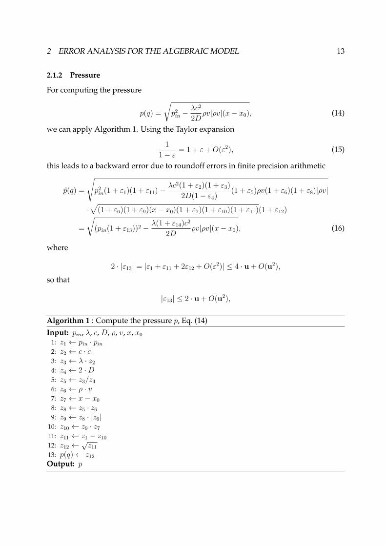
2.1.2 Pressure

For computing the pressure

p(q) =

√p2in −

λc2

2Dρv|ρv|(x− x0), (14)

we can apply Algorithm 1. Using the Taylor expansion

1

1− ε= 1 + ε+O(ε2), (15)

this leads to a backward error due to roundoff errors in finite precision arithmetic

p(q) =

√p2in(1 + ε1)(1 + ε11)−

λc2(1 + ε2)(1 + ε3)

2D(1− ε4)(1 + ε5)ρv(1 + ε6)(1 + ε8)|ρv|

·√

(1 + ε6)(1 + ε9)(x− x0)(1 + ε7)(1 + ε10)(1 + ε11)(1 + ε12)

=

√(pin(1 + ε13))2 −

λ(1 + ε14)c2

2Dρv|ρv|(x− x0), (16)

where

2 · |ε13| = |ε1 + ε11 + 2ε12 +O(ε2)| ≤ 4 · u +O(u2),

so that

|ε13| ≤ 2 · u +O(u2),

Algorithm 1 : Compute the pressure p, Eq. (14)

Input: pin, λ, c, D, ρ, v, x, x01: z1 ← pin · pin2: z2 ← c · c3: z3 ← λ · z24: z4 ← 2 ·D5: z5 ← z3/z46: z6 ← ρ · v7: z7 ← x− x08: z8 ← z5 · z69: z9 ← z8 · |z6|

10: z10 ← z9 · z711: z11 ← z1 − z1012: z12 ←

√z11

13: p(q)← z12Output: p


and

|ε14| = |ε2 + ε3 + ε4 + ε5 + ε6 + ε8 + ε6 + ε9 + ε7 + ε10 + ε11 + 2ε12 +O(ε2)|≤ 13 · u +O(u2).

As a next step, measurement errors are introduced for all parameters. For example, themeasurement error for the parameter x is denoted by εx. Continuing with Eq. (16), thisgives

p(q)2 = (pin(1 + εpin)(1 + ε13))2

− λ(1 + ελ)(1 + ε14)c2(1 + εc)

2

2D(1− εD)ρv|ρv|(1 + ερ)

2(1 + εv)2(x(1 + εx)− x0(1 + εx0))

= (pin(1 + ε15))2 − λ(1 + ε16)c

2

2Dρv|ρv|(x(1 + εx)− x0(1 + εx0)), (17)

with

|ε15| = |εpin + ε13 +O(ε2)| ≤ |εpin|+ 2 · u + h.o.t., (18)

and

|ε16| = |ελ + ε14 + 2εc + εD + 2ερ + 2εv +O(ε2)|≤ |ελ|+ 2 · |εc|+ |εD|+ 2 · |ερ|+ 2 · |εv|+ 13 · u + h.o.t. (19)

So for the backward error of p(q), considered as a function of pin, λ, x, and x0, we havethe expression

p(pin, λ, x, x0) = p(pin(1 + ε15), λ(1 + ε16), x(1 + εx), x0(1 + εx0)).

Now that the backward error is obtained, the relative error in p(q) due to perturbationsin the data q can be calculated and is given by

p(q)− p(q + ∆q)

p(q)=∂p(q)

∂pin

pinp(q)

∆pinpin

+∂p(q)

∂λ

λ

p(q)

∆λ

λ+∂p(q)

∂x

x

p(q)

∆x

x+∂p(q)

∂x0

x0p(q)

∆x0x0

+O((∆q)2

)=

(pinp(q)

)2

︸︷︷︸κpin (q)

ε15 −λc2ρ2v2(x− x0)

4Dp(q)2︸︷︷︸κλ(q)

ε16 −λc2ρ2v2x

4Dp(q)2︸︷︷︸κx(q)

εx +λc2ρ2v2x04Dp(q)2︸︷︷︸κx0 (q)

εx0

+ h.o.t.,

where κpin , κλ, κx, and κx0 are the individual relative condition numbers, Eq. (8). For therelative condition number κpin(q) with respect to pin it holds that


κpin(q) =

(pinp(q)

)2

> 1,

because p(q) =√p2in − λc2

2Dρv|ρv|(x− x0) <

√p2in = pin. Taking the nominal values qnom

as

pinnom = 2 · 105 (or 2 bar),λnom = 0.06,

cnom = 343,

Dnom = 1, (20)ρnom = 1,

vnom = 10,

xnom = 105 (or 100 km), andx0nom = 0,

gives an amplification factor of

κpin(qnom) = 8.5.

For the relative condition number κλ(q) it holds that κλ ≤ 1 if and only if

L = x− x0 ≤4Dp2in

3λc2ρ2v2.

Substituting the nominal values qnom, Eq. (20), yields

L ≤ 7.56 · 104.

With nominal values qnom in Eq. (20), in particular x0nom = 0, it holds that κx(q) = κλ(q)and κx0(q) = 0. The relative condition numbers κpin and κλ are given in Fig. 2 as afunction of the pipeline length L = x − x0. The remaining input parameters are fixedto the values in Eq. (20). This figure shows that the relative condition numbers growquickly with increasing pipeline length L. The two graphs have a vertical asymptote atL ≈ 113 km, as the pressure in this point is

p(qnom, x = 113, 331) = 404 Pa, (21)

which is approximately zero.

It can be concluded that the algebraic model can only be used safely for pipelines upto 60 km length. For pipelines longer than 60 km the pressure can not be computedaccurately as the relative condition number κpin is then larger than two. A more accuratemodel in the model hierarchy, see Sec. 1.1, should be chosen for the pipelines longer than60 km.


2.1.3 Temperature

To compute the temperature

T (q) = (Tin − Tw)e−kw

Dcvρv(x−x0) + Tw, (22)

Algorithm 2 can be applied. As every step introduces a relative error ε, the following

0 50 100 1500

2

4

6

8

10

12

14

Relative condition number κp

in

Pipeline length L [km]

κp

in

0 50 100 1500

1

2

3

4

5

6

7

Relative condition number κλ


κλ

Fig. 2: Individual relative condition numbers κpin and κλ with respect to pin and λ,respectively, for the pressure p, considered as a function of the pipeline lengthL = x−x0.

Algorithm 2 : Compute the temperature T , Eq. (22)

Input: Tin, Tw, kw, D, cv, ρ, v, x, x01: z1 ← Tin − Tw2: z2 ← D · cv3: z3 ← z2 · ρ4: z4 ← z3 · v5: z5 ← kw/z46: z6 ← x− x07: z7 ← z5 · z68: z8 ← e−z7

9: z9 ← z1 · z810: z10 ← z9 + Tw11: T (q)← z10Output: T


expression is obtained, using the Taylor series expansion in Eq. (15),

T (q) = [(Tin − Tw)(1 + ε1)e− kwDcv(1−ε2)ρ(1−ε3)v(1−ε4)

(1+ε5)(x−x0)(1+ε6)(1+ε7)(1 + ε8)(1 + ε9)

+ Tw](1 + ε10)

= (Tin(1 + ε11)− Tw(1 + ε11)) e− kw(1+ε12)

Dcvρv(x−x0) + Tw(1 + ε10)

=

(Tin(1 + ε11 −

TwTin

(ε11 − ε10))− Tw(1 + ε10)

)e−

kw(1+ε12)Dcvρv

(x−x0) + Tw(1 + ε10),

(23)

where

1 + ε11 = (1 + ε1)(1 + ε8)(1 + ε9)(1 + ε10),

1 + ε12 = (1 + ε2)(1 + ε3)(1 + ε4)(1 + ε5)(1 + ε6)(1 + ε7),

|ε10| ≤ u,

|ε11| = |ε1 + ε8 + ε9 + ε10 +O(ε2)| ≤ 4u +O(u2), and|ε12| = |ε2 + ε3 + ε4 + ε5 + ε6 + ε7 +O(ε2)| ≤ 6u +O(u2).

This leads to a backward error for T (q), considered as a function of Tin, Tw, and kw, givenby the expression

T (Tin, Tw, kw) = T

(Tin(1 + ε11 −

TwTin

(ε11 − ε10)), Tw(1 + ε10), kw(1 + ε12)

).

Including measurement errors for the input parameters, continuing with Eq. (23), gives

T (q) =

(Tin(1 + εTin)(1 + ε11 −

Tw(1 + εTw)

Tin(1− εTin)(ε11 − ε10))− Tw(1 + εTw)(1 + ε10)

)· e−

kw(1+εkw)(1+ε12)

D(1−εD)cv(1−εcv )ρ(1−ερ)v(1−εv)(x(1+εx)−x0(1+εx0 )) + Tw(1 + εTw)(1 + ε10)

= (Tin(1 + ε13)− Tw(1 + ε14)) e− kw(1+ε15)

Dcvρv(x(1+εx)−x0(1+εx0 )) + Tw(1 + ε14),

where

1 + ε13 = (1 + εTin)(1 + ε11 −Tw(1 + εTw)

Tin(1− εTin)(ε11 − ε10))

= 1 + εTin + ε11 −TwTin

(ε11 − ε10) +O(ε2),

1 + ε14 = (1 + εTw)(1 + ε10) = 1 + εTw + ε10 +O(ε2), and1 + ε15 = (1 + εkw)(1 + ε12)(1 + εD)(1 + εcv)(1 + ερ)(1 + εv) +O(ε2)

= 1 + εkw + ε12 + εD + εcv + ερ + εv +O(ε2).


This results in the backward error

T (Tin, Tw, kw, x, x0) = T (Tin(1 + ε13), Tw(1 + ε14), kw(1 + ε15), x(1 + εx), x0(1 + εx0)).

For the relative error in the temperature T (q) due to finite precision arithmetic and dataerrors, it holds that

T (q)− T (q)

T (q)=T (q)− T (q + ∆q)

T (q)

=

(∂T (q)

∂Tin

TinT (q)

)∆TinTin

+

(∂T (q)

∂Tw

TwT (q)

)∆TwTw

+

(∂T (q)

∂kw

kwT (q)

)∆kwkw

+

(∂T (q)

∂x

x

T (q)

)∆x

x+

(∂T (q)

∂x0

x0T (q)

)∆x0x0

+O((∆q)2

)=

Tin

Tin +(ekw(x−x0)Dcvρv − 1

)Tw︸︷︷︸

κTin (q)

ε13 +Tw − Twe−

kw(x−x0)Dcvρv

(Tin − Tw)e−kw(x−x0)Dcvρv + Tw︸︷︷︸

κTw (q)

ε14

− (Tin − Tw)(x− x0)kwDcvρv

(Tin + (e

kw(x−x0)Dcvρv − 1)Tw

)︸︷︷︸

κkw (q)

ε15 −(Tin − Tw)kwx

DcvρvT (q)e−

kw(x−x0)Dcvρv︸︷︷︸

κx(q)

εx

+(Tin − Tw)kwx0DcvρvT (q)

e−kw(x−x0)Dcvρv︸︷︷︸

κx0 (q)

εx0 +O((∆q)2

). (24)

We are interested, in whether the relative errors ε13, ε14, ε15, εx, and εx0 in the inputparameters are amplified in the relative error for the temperature T . To this end, thenominal values

Dnom = 1,

ρnom = 1,

vnom = 10,

Tinnom = 293,

Twnom = 283, (25)kwnom = 0.0341,

cvnom = 1700, andx0nom = 0,

are inserted in the individual relative condition numbers in Eq. (24). With x0nom = 0 itholds that κx0(qnom) = 0. The four remaining relative condition numbers are given in


Fig. 3 as a function of the pipeline length L = x − x0. The figure shows that all relativecondition numbers remain below one, which means that the relative errors in the inputparameters are not amplified. The relative condition numbers κkw and κx are so smallcompared with κTin and κTw , that they can be neglected.

0 50 100 1500.8

0.85

0.9

0.95

1

Relative condition number κT

in


κT

in

0 50 100 1500

0.05

0.1

0.15

0.2

Relative condition number κT

w


κT

w

0 50 100 1500

1

2

3

4

5

6x 10

−3Relative condition number κ

kw


κk

w

0 50 100 1500

1

2

3

4

5

6x 10

−3

Relative condition number κx


κx

Fig. 3: The individual relative condition numbers κTin , κTw , κkw , and κx for the temper-ature T , considered as a function of the pipeline length L = x− x0.


2.2 Statistical Analysis

A statistical analysis for the algebraic model in Eq. (10) is performed in this section. Thisanalysis is complementary to the theoretical analysis carried out in Sec. 2.1. It aims tostatistically validate the theoretical results obtained in Sec. 2.1. This is done by explicitlyperturbing the input parameters and calculating the corresponding output parametervalues. It gives direct insight in the sensitivity of the output parameters to perturba-tions in the input parameters. First, in Sec. 2.2.1, the statistical analysis is performedusing a Monte Carlo Simulation (MCS). This simulation has the advantage that the ac-curacy can be arbitrarily increased by enlarging the sample size. However, it has thedisadvantage that the sample size should be large to get reliable results, i.e., the com-putational complexity is high. Second, in Sec. 2.2.2, the statistical analysis is performedusing the Univariate Reduced Quadrature (URQ) Method. This method is characterizedby a small sample size, together with a fixed accuracy. The small sample size and thecorresponding low computational complexity allow us to calculate the sensitivity of theoutput parameters for many different pipeline lengths.

2.2.1 Monte Carlo Simulation

For this simulation, the input parameters q ∈ Rn are considered to be random variables.The mean µq of these variables is given by the nominal values in Eqs. (20) and (25). Thestandard deviation σq of the input parameters is set to 0.5% of the mean, so that for therelative standard deviation (rsd) it holds that σqi/µqi = 0.5% for every element qi of q.Then, samples are drawn from those distributions. For the sample size N we chooseN = 104. The mean µf and variance σ2

f of the output parameters f are approximatedusing the well-known formulas [5]

µfMCS =1

N

N∑i=1

f(qi) (26)

and

σ2fMCS

=1

N − 1

N∑i=1

[f(qi)− µfMCS ]2 . (27)

The error of these approximations is given by [11]

|µf − µfMCS| = O(1/√N) and |σ2

f − σ2fMCS| = O(1/

√N).

So, the accuracy can be arbitrarily increased, although the order of convergence is only1/2. The sample size depends on the desired accuracy of the output distribution. Notethat the error is independent of the problem dimension n, which makes a MCS unaf-fected by the “curse of dimensionality”.


The result of the simulation for the mass flux f1 in Eq. (11) is given in Fig. 4. It shows thatµf1 ≈ 10. The rsd for f1, σf1/µf1 , is equal to 0.7%. This corresponds with the theoreticalanalysis carried out in Sec. 2.1.1, which resulted in a relative error for f1 that is smallerthan or equal to the sum of the relative errors of the input parameters. Indeed, 0.7% ≤0.5% + 0.5%.

The result of the MCS for the pressure, Eq. (14), is given in Fig. 5. It shows the outputdistribution for both normally and uniformly distributed input parameters for severalpipeline lengths. There is basically no difference in the rsd of the pressure p betweennormally and uniformly distributed input parameters. The rsd of p grows quickly withincreasing pipeline length L. This corresponds with the analytical analysis in Sec. 2.1.2together with Fig. 2, where we also found that the relative condition numbers growquickly with increasing L.

For the temperature T in Eq. (22) the result of the MCS is given in Fig. 6. There is nodifference in the rsd of T between normally and uniformly distributed input parame-ters, although the shape of the output distribution is different. With increasing pipelinelength L, the rsd of T decreases slightly. This is in line with the theoretical analysis car-ried out in Sec. 2.1.3 and with Fig. 3, where we found that all relative condition numbersstay below one for all pipeline lengths, i.e., the relative errors of the input parametersare not amplified.

2.2.2 URQ Method

The URQ method [11] is developed to find an appropriate trade-off between compu-tational complexity and accuracy. Whereas the MCS method in Eqs. (26) and (27) isusually performed with a sample size N of approximately 104, the URQ method onlyutilizes a sample size of N = 2n + 1, where n is the number of input parameters. This

9.5 10 10.50

1000

2000

3000

4000

f1

Fre

qu

en

cy

Fig. 4: Result of a MCS for the mass flux f1, Eq. (11). The input parameters are normallydistributed with a rsd of 0.5%.


makes the URQ method computationally much less expensive than the MCS method,especially for computationally demanding analysis codes, i.e., when the evaluation off(q) is computationally expensive. The mean µf and the variance σ2

f of an output pa-rameter f are approximated in the URQ method using the following quadrature formu-

1.85 1.9 1.95 2

x 105

0

500

1000

1500

2000

2500

3000L = 10 km, normal input dist.

p, σp/µ

p = 0.55%

Fre

quency

1.85 1.9 1.95 2

x 105

0

500

1000

1500L = 10 km, uniform input dist.

p, σp/µ

p = 0.55%

Fre

quency

1.55 1.6 1.65 1.7

x 105

0

500

1000

1500

2000

2500


p, σp/µ

p = 0.89%

Fre

quency

1.55 1.6 1.65 1.7

x 105

0

500

1000

1500


p, σp/µ

p = 0.89%

Fre

quency

1.1 1.2 1.3 1.4

x 105

0

500

1000

1500

2000

2500


p, σp/µ

p = 1.9%

Fre

quency

1.1 1.2 1.3 1.4

x 105

0

500

1000

1500

2000

2500


p, σp/µ

p = 1.9%

Fre

quency

4 6 8 10

x 104

0

500

1000

1500

2000

2500


p, σp/µ

p = 7.6%

Fre

quency

4 6 8 10

x 104

0

500

1000

1500

2000

2500


p, σp/µ

p = 7.6%

Fre

quency

Fig. 5: Result of a MCS for the pressure p, Eq. (14), for different pipeline lengths. Theinput parameters are either normally or uniformly distributed with a rsd of 0.5%.

285 290 295 3000

1000

2000

3000


T, σT/µ

T = 0.49%

Fre

quency

285 290 295 3000

500

1000


T, σT/µ

T = 0.49%

Fre

quency

285 290 295 3000

500

1000

1500

2000

2500


T, σT/µ

T = 0.46%

Fre

quency

285 290 295 3000

500

1000


T, σT/µ

T = 0.47%

Fre

quency

285 290 295 3000

500

1000

1500

2000

2500


T, σT/µ

T = 0.44%

Fre

quency

285 290 295 3000

500

1000


T, σT/µ

T = 0.44%

Fre

quency

285 290 295 3000

500

1000

1500

2000

2500


T, σT/µ

T = 0.42%

Fre

quency

285 290 295 3000

500

1000


T, σT/µ

T = 0.42%

Fre

quency

Fig. 6: Result of a MCS for the temperature T , Eq. (22), for different pipeline lengths.The input parameters are either normally or uniformly distributed with a rsd of 0.5%.


las [11]:

µfURQ(µq) = W0f(µq) +n∑i=1

Wi

[f(q+i )

h+i− f(q−i )

h−i

](28)

and

σ2fURQ

(µq) =n∑i=1

{W+i

[f(q+i )− f(µq)

h+i

]2+W−

i

[f(q−i )− f(µq)

h−i

]2+ W±

i

[f(q+i )− f(µq)][f(q−i )− f(µq)]

h+i h−i

}, (29)

with appropriately chosen sampling points qi, weights Wi, and scaling parameters hi,which can be found in [11]. The error in these approximations is given by [11]

|µf − µfURQ| = O(σ4q) and |σ2

f − σ2fURQ| = O(σ4

q),

where O(σ4q) denotes all terms of order 4 and higher, i.e., terms proportional to σ2

qiσ2qj

,σ3qiσ2qj

, etc., for i, j ∈ {1, . . . , n}.

This efficient uncertainty propagation technique enables us to calculate the rsd of thepressure p and the temperature T for many different pipeline lengths L. The mean ofthe remaining input parameters is set to the nominal values in Eqs. (20) and (25). Again,it holds for the rsd σqi/µqi = 0.5% for every input parameter qi of q. The mass flux f1 isnot considered here, because it is constant with respect to L and can be found in Fig. 4.

The result of this simulation for p and T can be found in Fig. 7. We observe the samebehavior as in the MCS in Sec. 2.2.1 and in the theoretical analysis in Sec. 2.1, namely

0 20 40 60 80 100 1200

1

2

3

4

5

6

7

8


Rela

tive s

tandard

devia

tion σ

p/

µp [%

]

URQ Method for the pressure p

0 20 40 60 80 100 1200.4

0.41

0.42

0.43

0.44

0.45

0.46

0.47

0.48

0.49

0.5


Rela

tive s

tandard

devia

tion σ

T/

µT [%

]

URQ Method for the temperature T

Fig. 7: The relative standard deviation of the pressure (left) and the temperature (right)as a function of the pipeline length. The rsd of the input parameters is 0.5%.

the uncertainty in the pressure p grows quickly for increasing pipeline length L and theuncertainty in the temperature T decreases slightly for increasing L.

2.3 Simplification from Temperature Dependent to Isothermal Alge-braic Model

The temperature dependent algebraic model, given by Eqs. (3), (4), and (5), can be sim-plified by assuming the temperature T to be constant. In this way, the isothermal al-gebraic model given by Eqs. (3) and (4) is obtained. The first order approximation ofthe relative error that is made in this simplification is given by Eq. (7), where the tem-perature T is inserted for f . The vector relative condition number, Eq. (9), of T for thenominal values qnom in Eq. (25) together with xnom = 7 · 104 (70 km) is given by

κ(qnom) =

∣∣∣∂T∂ρ (qnom) ρT (qnom)

∣∣∣∣∣∣∂T∂v (qnom) vT (qnom)

∣∣∣∣∣∣ ∂T∂D (qnom) DT (qnom)

∣∣∣∣∣∣∂T∂x (qnom) xT (qnom)

∣∣∣∣∣∣ ∂T∂x0 (qnom) x0T (qnom)

∣∣∣∣∣∣ ∂T∂Tin (qnom) TinT (qnom)

∣∣∣∣∣∣ ∂T∂Tw (qnom) TwT (qnom)

∣∣∣∣∣∣ ∂T∂kw (qnom) kwT (qnom)

∣∣∣∣∣∣ ∂T∂cv (qnom) cvT (qnom)

∣∣∣

T

=

0.0042

0.0042

0.0042

0.0042

0

0.8729

0.1271

0.0042

0.0042

T

.

It follows that only perturbations in the parameter Tin create an equivalent relative errorin the temperature T . Perturbations in the other input parameters only cause a smallrelative error in T . This means that if the input temperature Tin is not subject to change,the temperature can safely be set constant. If, however, the input temperature changes,for example for different pipelines, the temperature can not be set constant and thetemperature dependent algebraic model should be chosen.

We now analyse the case where in the formula for the temperature

T (x) = (Tin − Tw)e−kw

Dcvρv(x−x0) + Tw

only the parameter x is variable and the other variables are fixed. We assume that thelength of the pipeline L is 100 km and that x0 = 0. The maximum absolute error Eabs

24


that is made when the temperature is set constant is then given by

maxx∈[0,100 km]

Eabs = maxx∈[0,100 km]

|T −T (x)| = maxx∈[0,100 km]

|T − (Tin−Tw)e−kw

Dcvρv(x−x0)−Tw|. (30)

The maximum relative error Erel that is made when T is set constant is given by

maxx∈[0,100 km]

Erel = maxx∈[0,100 km]

|T − T (x)||T (x)|

= maxx∈[0,100 km]

|T − (Tin − Tw)e−kw

Dcvρv(x−x0) − Tw|

|(Tin − Tw)e−kw

Dcvρv(x−x0) + Tw|

.

(31)One possibility to set the temperature constant would be to measure the temperature atthe beginning and at the end of the pipeline and to take the average value, i.e.,

T =T (0) + T (100 km)

2.

Then, the graphs for the variable and the constant temperature for the nominal valuesqnom in Eq. (25) are given in Fig. 8. For these nominal values the maximum absoluteerror in Eq. (30) is Eabs = 0.909 and the maximum relative error in Eq. (31) is Erel =0.0031. This is a small relative error, such that in this case the temperature can safely beset constant.

0 20 40 60 80 100291

291.5

292

292.5

293

Tem

pera

ture

T


T variable

T constant

Fig. 8: Graphs for variable temperature with the nominal values in Eq. (25) and forconstant temperature as the average of T (0) and T (100 km).

3 Conclusion

The error analysis for the mass flux results in an error that is smaller than or equal to thesum of the errors of the two input parameters. Both the theoretical and the statisticalanalysis for the pressure show that the error grows quickly with increasing pipelinelength, from which it is concluded that the algebraic model can only be used safely forpipelines up to 60 km length. On the other hand, the error in the temperature decreasesslightly with increasing pipeline length.

Finally, it is shown in this work that only if the pipeline input temperature is not subjectto change, the temperature can safely be set constant and the isothermal algebraic modelcan be used. Otherwise, the temperature dependent algebraic model should be used tosimulate the gas flow.

Acknowledgements

The authors would like to thank both Dr. A. Miedlar for the inspiring discussions andthe Deutsche Forschungsgemeinschaft for their support within Projekt B03 in the Son-derforschungsbereich / Transregio 154 Mathematical Modelling, Simulation and Optimiza-tion using the Example of Gas Networks.

26

References

[1] Energy Consumption in Germany. http://www.bmwi.de/BMWi/Redaktion/Binaer/Energiedaten/energiegewinnung-und-energieverbrauch2-primaerenergieverbrauch.xls. Accessed: 2014-11-05.

[2] Gas pipelines in Europe. https://www.bdew.de/internet.nsf/res/EM_2012E_S_24-25.jpg/$file/EM_2012E_S_24-25.jpg. Accessed: 2014-11-05.

[3] M. Bollhöfer and V. Mehrmann. Numerische Mathematik: Eine Projektorientierte Ein-führung Für Ingenieure, Mathematiker und Naturwissenschaftler. Vieweg Studium;Grundkurs Mathematik. Vieweg+Teubner Verlag, 2004.

[4] J. Brouwer, I. Gasser, and M. Herty. Gas pipeline models revisited: Model hierar-chies, nonisothermal models, and simulations of networks. Multiscale Modeling &Simulation, 9(2):601–623, 2011.

[5] F.M. Dekking, C. Kraaikamp, H.P. Lopuhaä, and L.E. Meester. A Modern Intro-duction to Probability and Statistics: Understanding Why and How. Springer Texts inStatistics. Springer London, 2010.

[6] P. Domschke, O. Kolb, and J. Lang. Adjoint-based control of model and discretisa-tion errors for gas and water supply networks. In X. Yang and S. Koziel, editors,Computational Optimization and Applications in Engineering and Industry, pages 1–17.Springer, 2011.

[7] P. Domschke, O. Kolb, and J. Lang. Adjoint-based control of model and discreti-sation errors for gas flow in networks. Int. J. Mathematical Modelling and NumericalOptimisation, 2(2):175–193, 2011.

[8] N.J. Higham. Accuracy and Stability of Numerical Algorithms. Society for Industrialand Applied Mathematics, 1996.

[9] M. Konstantinov, D.W. Gu, V. Mehrmann, and P. Petkov. Perturbation Theory forMatrix Equations. Studies in Computational Mathematics. Elsevier Science, 2003.

[10] R.J. LeVeque. Finite Volume Methods for Hyperbolic Problems. Cambridge Texts inApplied Mathematics. Cambridge University Press, 2002.

[11] M. Padulo, M. S. Campobasso, and M. D. Guenov. Novel Uncertainty PropagationMethod for Robust Aerodynamic Design. AIAA Journal, 49(3):530–543, 2011.

[12] J.R. Rice. Numerical Methods, Software, and Analysis. Academic Press, 1993.

27

http://www.bmwi.de/BMWi/Redaktion/Binaer/Energiedaten/energiegewinnung-und-energieverbrauch2-primaerenergieverbrauch.xls



https://www.bdew.de/internet.nsf/res/EM_2012E_S_24-25.jpg/$file/EM_2012E_S_24-25.jpg

https://www.bdew.de/internet.nsf/res/EM_2012E_S_24-25.jpg/$file/EM_2012E_S_24-25.jpg

error analysis for the euler equations in purely algebraic

Documents