erdc/gsl tr-07-25, geophysical surveys for assessing … · foundation conditions, feather river...
TRANSCRIPT

ERD
C/G
SL T
R-07
-25
Flood and Coastal Storm Damage Reduction Research Program Geophysical Surveys for Assessing Levee Foundation Conditions, Feather River Levees, Marysville/Yuba City, California
José L. Llopis and Janet E. Simms September 2007
Geo
tech
nica
l and
Str
uctu
res
Labo
rato
ry
Approved for public release; distribution is unlimited.
Flood and Coastal Storm Damage Reduction (FCSDR) Research Program
ERDC/GSL TR-07-25 September 2007
Geophysical Surveys for Assessing Levee Foundation Conditions, Feather River Levees, Marysville/Yuba City, California
José L. Llopis and Janet E. Simms Geotechnical and Structures Laboratory U.S. Army Engineer Research and Development Center 3909 Halls Ferry Road Vicksburg, MS 39180-6199
Final report Approved for public release; distribution is unlimited.
Prepared for Headquarters, U.S. Army Corps of Engineers Washington, DC 20314-1000
ERDC/GSL TR-07-25 ii
Abstract: Effective flood and coastal storm emergency response depends on the ability of emergency managers to obtain information on the condition of flood-damage reduction structures in near real-time. This report describes the results of a geophysical study performed to determine the potential for geophysical methods to provide supplemental geologic data between existing soil borings in a rapid fashion in an area of complex geology. The geophysical study was conducted along 10 km of landside levee toe adjacent to the Feather River, approximately 5 km south of Marysville/Yuba City, CA. Electromagnetic induction, capacitively coupled electrical resistivity, and direct current electrical resistivity survey methods were used to conduct the geophysical study. Survey results were used to classify soil type to depths of approximately 60 m.
DISCLAIMER: The contents of this report are not to be used for advertising, publication, or promotional purposes. Citation of trade names does not constitute an official endorsement or approval of the use of such commercial products. All product names and trademarks cited are the property of their respective owners. The findings of this report are not to be construed as an official Department of the Army position unless so designated by other authorized documents. DESTROY THIS REPORT WHEN NO LONGER NEEDED. DO NOT RETURN IT TO THE ORIGINATOR.

ERDC/GSL TR-07-25 iii
Contents Figures and Tables.................................................................................................................................iv
Preface.....................................................................................................................................................v
Unit Conversion Factors........................................................................................................................vi
1 Introduction..................................................................................................................................... 1 Background .............................................................................................................................. 1 Purpose and scope .................................................................................................................. 3 Study area................................................................................................................................. 3 Geologic setting........................................................................................................................ 3
2 Geophysical Test Principles and Field Procedures..................................................................... 6 Electromagnetic surveys .......................................................................................................... 6 dc electrical resistivity surveys ..............................................................................................10 Capacitively coupled conductivity surveys............................................................................12
3 Geophysical Test Results, Interpretation and General Discussion.........................................15 Geophysical test results.........................................................................................................15
EM31 and EM34 results............................................................................................................15 GEM-2 results.............................................................................................................................18 OhmMapper results ...................................................................................................................20 SARIS results ..............................................................................................................................21
Interpretation of results .........................................................................................................22 General discussion.................................................................................................................26
4 Conclusions and Recommendations .........................................................................................30 Conclusions ............................................................................................................................30 Recommendations .................................................................................................................32
References............................................................................................................................................33
Appendix A: EM31 and EM34 Electrical Conductivity Results, Plan Views .................................34
Appendix B: EM31 and EM34 Electrical Conductivity Results, Profiles.......................................54
Appendix C: EM31 and EM34 Electrical Conductivity Results, Pseudosections.........................72
Appendix D: GEM-2 Electrical Conductivity Results, Profiles.........................................................79
Appendix E: OhmMapper Electrical Conductivity Results, Depth Sections..................................97
Appendix F: SARIS Electrical Conductivity Results, Depth Sections...........................................107
Report Documentation Page

ERDC/GSL TR-07-25 iv
Figures and Tables
Figures
Figure 1. Location and layout of geophysical survey line, east bank, land side toe of the Feather River............................................................................................................................................... 5 Figure 2. Sled-mounted Geonics Ltd. EM31 EM induction instrument being used during a typical survey. ............................................................................................................................................. 8 Figure 3. Geonics Ltd. EM34 EM induction instrument being towed by a vehicle collecting “continuous” data. ................................................................................................................................... 10 Figure 4. A sled-mounted Geophex GEM-2 multi-frequency EM induction instrument being prepared for surveying.............................................................................................................................11 Figure 5. The Dipole-Dipole electrical resistivity profile array............................................................... 11 Figure 6. SARIS dc electrical resistivity survey arrangement. ..............................................................13 Figure 7. Geometrics OhmMapper capacitively coupled resistivity system being vehicle-towed. ........................................................................................................................................................ 14 Figure 8. Interpreted soil distribution map, UTM 4328000 to 4325000. ........................................22 Figure 9. Interpreted soil distribution map, UTM 4325000 to 4322000. ........................................23 Figure 10. Interpreted soil distribution map, UTM 4322000 to 4319000. ......................................23 Figure 11. Example of a portion of EM34 data plot posted on the Integrated Levee Assessment Utility Web site. ...................................................................................................................29
Tables
Table 1. Electrical resistivity values of some common rocks and minerals. ........................................ 7 Table 2. EM31 and EM34 statistical values. ......................................................................................... 16 Table 3. GEM-2 statistical values............................................................................................................19 Table 4. Geophysical anomaly interpretation. ....................................................................................... 24
ERDC/GSL TR-07-25 v
Preface
This report describes a research study commissioned by the U.S. Army Corps of Engineers’ Emergency Management Technologies focus area of the Flood and Coastal Storm Damage Reduction (FCSDR) Research Prog-ram and conducted by the U.S. Army Engineer Research and Development Center (ERDC) to determine the feasibility of using surface-based geo-physical surveys to rapidly map and characterize soils along the toe of a levee. The work was performed during the period 14–21 June 2006 along a selected portion of the Feather River east (left) bank levee approximately 5 km south of Marysville/Yuba City, CA. Dr. Kathleen D. White, ERDC Cold Regions Research Engineering Laboratory, is the Program Manager for the FCSDR Emergency Management Technologies focus area.
The research described herein was conducted by José L. Llopis and Dr. Janet E. Simms of ERDC Geotechnical and Structures Laboratory (GSL). This report was prepared by Llopis and Dr. Simms under the general supervision of Dr. Lillian D. Wakeley, former Chief, Engineering Geology and Geophysics Branch; Dr. Robert L. Hall, Chief, Geosciences and Structures Division; Dr. William P. Grogan, Deputy Director, GSL; and Dr. David W. Pittman, Director, GSL.
COL Richard B. Jenkins was Commander and Executive Director of ERDC. Dr. James R. Houston was Director.

ERDC/GSL TR-07-25 vi
Unit Conversion Factors
Multiply By To Obtain
feet 0.3048 meters
miles (U.S. statute) 1,609.347 meters

ERDC/GSL TR-07-25 1
1 Introduction Background
Levees are a fundamental part of many flood-damage reduction projects that protect life and property. The condition and performance of levees in emergency flooding situations are of utmost importance. The U.S. Army Corps of Engineers (USACE) has conducted research and development activities related to levees in a number of research programs, including the Innovative Flood Protection Program and its successor, the Technologies and Operational Innovations for Urban Watershed Networks (TOWNS) Research Program. Currently, research related to levee condition evalua-tion and assessment is being conducted under the auspices of the Emer-gency Management Technologies focus area of the Flood and Coastal Storm Damage Reduction (FCSDR) research program. A primary objective of this research is to develop the capability to rapidly obtain information about levee conditions and convey the data to decision-makers during emergency operations, particularly in cases where levee failure is possible.
Levee failures are governed in large part by the soils that form the embankments and their foundations. Failure of the levee occurs as a result of the river scouring the toe of the levee, causing the embankment to col-lapse into the channel; by overtopping of the embankment; and by seepage and piping through the embankment or its foundation. Water seepage through the levee embankment (through-seepage) can produce internal erosion of the levee soils. Foundation problems in levees usually are caused by under-seepage and are related to geologic conditions at the site.
Through-seepage is not normally a major concern for levees constructed of clay soils unless flood stage is maintained long enough that the embank-ment becomes saturated; or when defects in the levee, such as animal bur-rows or desiccation cracks, allow concentrated flows. Seepage through levees consisting of silt and sand can produce erosion at the landside slope and lead to breaching of the levee if the seepage remains uncontrolled.
Seepage of water beneath a levee constructed on a highly erodible founda-tion of silt, sand, or gravel deposits, is more critical than through-seepage. Identifying erodible foundation soils is an important step in preventing bank failures. Because floodplain deposits underlie levees, knowledge of

ERDC/GSL TR-07-25 2
the geology of local floodplain deposits is an important consideration in flood-control management. Levee systems are often built atop highly per-meable, relatively coarse-grained river deposits. These sediments repre-sent old channels and courses of the river system abandoned during the river’s history of meandering over the floodplain. These coarse-grained deposits represent the most likely locations for under-seepage in levee systems.
It is imperative that geologic features be identified in the earliest stages of a levee condition assessment so that other exploratory methods can be used to confirm their existence and map their distribution. Knowledge of fluvial processes and the ability to recognize depositional environments in the geologic record are the key to identifying locations along modern lev-ees where under-seepage has the greatest potential to occur. To gain more information about the foundation materials, borings are usually placed at predetermined distances, sometimes hundreds of meters apart, along the levee axis. Through the performance of Standard Penetration Testing (SPT) during the drilling of borings, along with laboratory testing of soil samples, engineering soil properties as a function of depth at a given bor-ing location are obtained; however, soils information between borings must be interpolated. In some geologic conditions, where there are gradual or rather predictable soil changes, the interpolations may be adequate. In areas where the geology is more complex, interpolating the soil properties or conditions between borings may not be adequate. In the case of a geologically complex site, many more closely spaced borings would have to be placed to define the subsurface conditions with sufficient detail for meaningful engineering judgment.
As an alternative to drilling very closely spaced borings, surface geophysi-cal testing can be conducted between the more widely spaced borings to provide cost-effective geologic information. In 2003, personnel of the U.S. Army Engineer Research and Development Center (ERDC) conducted a proof of principle study along U.S. International Boundary and Water Commission levees in the Lower Rio Grande Valley of Texas (Dunbar et al. 2003). The study consisted of first conducting helicopter-borne electro-magnetic surveys along the levees to obtain an overall assessment of soil conditions of the levees and their foundation materials. Anomalous areas were identified and investigated in greater detail using ground-based geo-physical surveys, a cone penetrometer equipped with an electrical resistiv-ity probe, and soil sampling. The study concluded that the method is eco-

ERDC/GSL TR-07-25 3
nomical and reliable for assessing materials and condition of levees and their foundations.
Purpose and scope
Potential failure of levees in the Sacramento-San Joaquin delta of Califor-nia has been identified as a critical engineering problem (Reid 2005, Hess and Sills 2004). Levees along the Feather River have experienced under-seepage during high-water events. Because of the complex geology in this area, it is difficult to predict where under-seepage is likely to occur, and thus where preventative or emergency measures should be prioritized. The purpose of this study was to determine the potential of geophysical meth-ods to provide supplemental geologic data between existing borings rap-idly, as would be desired for emergency situations, in a more complex geologic setting than where the concept was previously tested.
This report describes the results of a geophysical study conducted along a 10-km stretch of the Feather River levee south of Marysville/Yuba City, CA. The study was funded by the USACE’s Emergency Management Tech-nologies focus area of the FCSDR research program.
Study area
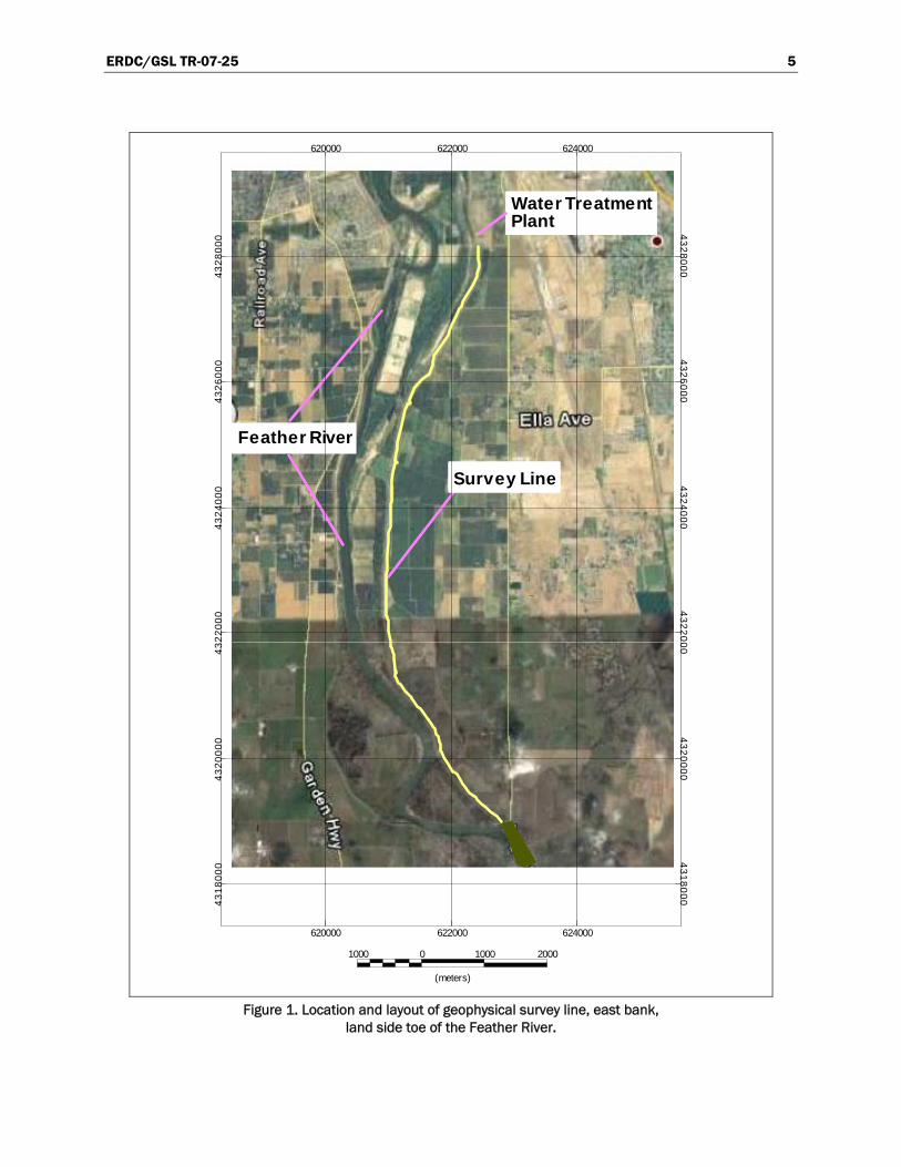
The study was conducted along the landside (L/S) levee toe of the east bank of Feather River (Figure 1). The northern end of the site was located approximately 5 km south of Marysville, CA. The survey site extended south from the water treatment plant, located approximately 2 km south of Island Avenue, to just north of the Star Bend boat ramp. The north and south ends of the survey line correspond to approximate USACE Sta. 434+00 and Sta. 106+00, respectively. Positioning is also expressed in this report in river miles (RM). The north and south ends of the survey line correspond to approximate RM 23.8 and 17.5, respectively. The site is located within the Three Rivers Levee Improvement Authority’s Reclama-tion District 784.
Geologic setting
The study area lies within the upper Sacramento Valley portion of the Great Valley geomorphic province of California. The Sacramento Valley lies between the northern Coast Range to the west and the northern Sierra Nevada to the east, and has been a depositional basin throughout most of
ERDC/GSL TR-07-25 4
the late Mesozoic and Cenozoic time. A vast accumulation of sediments was deposited during cyclic transgressions and regressions of a shallow sea which once inundated the valley. A thick sequence of clastic sedimen-tary rock units, derived from erosion of the adjoining highlands from the Late Jurassic to the Pleistocene, and Tertiary volcanics, form the bedrock units now deeply buried in the mid-basin areas of the valley. Late Pleisto-cene and Holocene (Recent) alluvial deposits now cover the area, consist-ing of reworked fan and stream material that were deposited by streams prior to the construction of the existing levees (Bookman-Edmonston 2006).
Levees in the upper Sacramento Valley were built on sedimentary deposits that reflect the changes in natural processes caused by human activity. The most recent deposits are sediments generated by hydraulic mining opera-tions in the Sierra Nevada during the mid 1800s. These sediments cover portions of the floodplain with a thickness estimated to range from 3 to 5 m. The main sediment influx occurred between 1853 and 1884, but the maximum aggradation on nearby Yuba River at Marysville was delayed until 1905, where a total of nearly 6.5 m of aggradation was observed. By the late 1860s, aggradation was so extreme that the beds of the Yuba and Feather Rivers were higher than the city streets in Marysville. After mining ceased, the sediment supply was dramatically reduced and Feather River began to incise into the deposited hydraulic mining sediment. Incision continued until the 1960s when the bed began to rest upon pre-hydraulic material that was more resistant to erosion. As a result of the rapid aggradation and subsequent incision, the banks of Feather River are principally composed of hydraulic mining material. The lowest mining deposits (called slickens) are relatively resistant to erosion whereas the upper mining materials are relatively less cohesive and more erodible. Thus, levees were constructed on foundations that are less than ideal in that the materials are coarse grained and laterally discontinuous, an envi-ronment in which interpolation between borings can be meaningless. Beneath the mining deposits, the upper native alluvial materials are relatively resistant to erosion, but they are underlain by less erosion resis-tant sediments (USACE 2006).
ERDC/GSL TR-07-25 5
1000 0 1000 2000
(meters)
Survey Line
Water TreatmentPlant
Feather River
4318
000
4320
000
4322
000
4324
000
4326
000
4328
000
43180004320000
43220004324000
43260004328000
620000 622000 624000
620000 622000 624000
Figure 1. Location and layout of geophysical survey line, east bank,
land side toe of the Feather River.
ERDC/GSL TR-07-25 6
2 Geophysical Test Principles and Field Procedures
This section provides a description of the surface geophysical methods and field procedures used for this study. The geophysical methods used include electromagnetic (EM) induction, capacitively coupled electrical resistivity (CCR), and direct current (dc) electrical resistivity.
Geophysical measurements were acquired along a survey line adjacent to the levee toe. The measurements were interpreted to infer lateral and vertical geologic changes beneath the survey line. Also, anomalous areas, which are departures from background conditions, were noted for further exploration.
Each geophysical method uses different physical principles to determine the electrical properties of the subsurface materials. Therefore, each sur-vey method is affected differently by the subsurface material properties and, consequently, each survey type may indicate different anomaly loca-tions. When the surveys are completed, anomalies may be identified for each geophysical method. By using different geophysical methods, areas considered for future exploration can be prioritized on the basis of the number of surveys that agree that a particular location is anomalous. For example, if three different survey methods indicate that a certain area is anomalous, then that area is given a higher priority for future exploration over an area that is considered anomalous on the basis of only one survey method.
Electromagnetic surveys
EM induction is used to measure the apparent electrical conductivity (inverse of electrical resistivity) of subsurface materials and also for detecting buried metallic items. Electrical conductivity is a measure of the degree to which the soil conducts an electrical current and can be used to infer geologic materials and the location of the water table. Conductivity values vary over several orders of magnitude depending on the type of earth material (Table 1). Major factors influencing the conductivity mea-surement are the amount of pore fluid present, the salinity of the pore fluid, the presence of conductive minerals, and the amount of fracturing.

ERDC/GSL TR-07-25 7
Table 1. Electrical resistivity values of some common rocks and minerals.
Material Resistivity, Ω-m Conductivity, milliSiemens/m (mS/m)
Igneous and Metamorphic Rocks Granite 5×10³ – 106 0.001 – 0.2 Basalt 103 – 106 0.001 – 1 Slate 6×10² – 4×10⁷ 2.5×10⁻⁵ – 1.7 Marble 102 – 2.5×10⁸ 4×10⁻⁶ – 10 Quartzite 102 – 2×10⁸ 5×10⁻⁶ – 10
Sedimentary Rocks Sandstone 8 – 4×10³ 0.25 – 125 Shale 20 – 2×10³ 0.5 – 50 Limestone 50 – 4×10² 2.5 - 20
Soils and Waters Clay 1 – 1000 1 – 1000 Alluvium 10 – 800 1.25 – 100 Groundwater (fresh) 10 – 100 10 – 100 Sea water 0.2 5000 Source: Keller and Frischknecht 1966.
Table 1 gives the conductivity values of common rocks and soil materials. Sedimentary rocks, because of their higher porosity and greater water con-tent, have higher conductivity values than intact igneous and metamorphic rocks. Wet soils and groundwater have even higher conductivity values. Clayey soil normally has a higher conductivity than a sandy soil (Locke 2000a).
The instrumentation used to measure soil conductivity consists of a trans-mitter (Tx) and receiver (Rx) coil separated by a certain distance. An alter-nating current is passed through the Tx coil, thus generating a primary time varying magnetic field. This primary field induces eddy currents in subsurface conductive materials. The induced eddy currents are the source of a secondary magnetic field, which is detected by the Rx coil along with the primary field.
Two components of the induced magnetic field are measured by the EM system. The first is the quadrature phase, sometimes referred to as the out-of-phase or imaginary component. Apparent ground terrain conduc-tivity is determined from the quadrature component. Disturbances in the subsurface caused by compaction, filled-in abandoned channels, soil removal and fill activities, buried objects, or voids may produce
ERDC/GSL TR-07-25 8
conductivity readings different from background values, thus indicating anomalous areas. The inphase component is very sensitive to metallic objects and, therefore, is useful when looking for buried metal such as metal rails, rebar, or electrical wires.
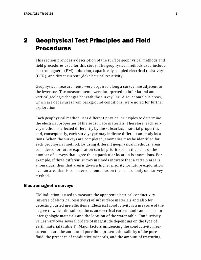
Geonics Ltd. EM31 and EM34 and a Geophex GEM-2 EM induction instrument were used in this investigation. The Tx and Rx coils for the EM31 were set at a fixed distance of 3.67 m. The EM31 has a nominal depth of investigation of about 6 m. The EM31 was placed on an electri-cally non-conductive sled and towed behind a vehicle along the survey line at a normal walking speed to acquire continuous (approximately every 0.3 m) data. The data were transmitted to an external logger via an RS-232 data link, thus allowing the unit to be integrated into a GPS- (global posi-tioning system) based survey system. A Trimble AG-132 GPS, in conjunc-tion with the Omnistar satellite differential positioning information ser-vice, was used to obtain sub-meter positioning accuracy. The data can be plotted in profile form showing conductivity values versus distance. The EM31 is shown in operation in Figure 2.
Figure 2. Sled-mounted Geonics Ltd. EM31 EM induction instrument
being used during a typical survey.
GPS Antenna
Data Recorder
EM31
GPS Receiver
ERDC/GSL TR-07-25 9
Unlike the EM31 with a fixed coil separation, the EM34 can be operated at Tx-Rx coil separations of 10, 20, or 40 m. The greater the Tx-Rx coil sepa-ration, the greater is the depth of investigation. EM34 data are collected in the vertical dipole mode (coils parallel to the ground surface) or in the horizontal dipole mode (coils perpendicular to the ground surface and coplanar). The vertical dipole mode allows for a greater depth of investi-gation and is less sensitive to near-surface materials. For this investiga-tion, the vertical dipole mode and coil separations of 10, 20, and 40 m were used, which allows for nominal depths of exploration of about 15, 30, and 60 m, respectively (McNeil 1980). Sleds were specially designed and constructed for this study using electrically non-conductive materials. The sled system allows the EM34 coils to sample data several times per second while being towed along the survey line. The sled system consists of three sleds, one each for the EM34 transmitter and receiver coils and one sled for the GPS placed halfway between the other two sleds. Ropes were used between the sleds to keep them a constant distance apart during the sur-vey. Figure 3 shows the EM34 in operation. Data along the profile lines were collected approximately every 0.3 m. In contrast, a hand-carried EM34 usually results in coarser (larger) data spacing.
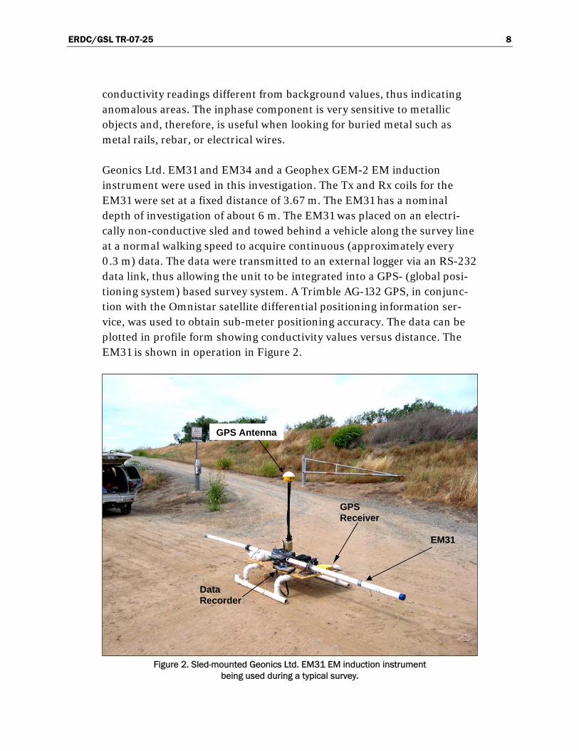
The GEM-2 is a handheld, digital, multi-frequency EM induction instru-ment (Won 2003). It operates in a specified frequency range of 330 Hz to 48 kHz with a waveform containing multiple frequencies. The GEM-2 con-tains Tx and Rx coils separated by 1.67 m (Figure 4). It can also collect data in the horizontal or in the vertical dipole mode. A selectable set of frequencies is used to measure changes in electrical conductivity as the instrument is moved along the survey line. A GPS was used with the GEM-2 to provide real-time position information. The exploration depth of EM instruments varies as a function of frequency and ground conduc-tivity. All other factors being equal, low frequency EM signals have greater exploration depths than higher frequency signals. For a given frequency, resistive ground has a greater exploration depth than conductive ground (Keller and Frischknecht 1966, Huang 2005). Therefore, the 330-Hz data will theoretically have a greater exploration depth than the 48-kHz data. The program WinGEM, available from Geophex, was used to convert the GEM-2 quadrature and inphase data to units of electrical conductivity.

ERDC/GSL TR-07-25 10
Figure 3. Geonics Ltd. EM34 EM induction instrument being towed by a
vehicle collecting “continuous” data.
dc electrical resistivity surveys
Electrical resistivity measurements are made by injecting current into the ground through two current electrodes (C1 and C2) and measuring the resulting voltage difference at two potential electrodes (P1 and P2). From the current and voltage values, an apparent resistivity value is calculated. The calculated resistivity value is not the true resistivity of the subsurface, but an apparent value because the subsurface is non-homogeneous. The relationship between apparent and true resistivity is complex. A mathematical analysis or an inversion of the measured apparent resistivity values using a computer program is performed to determine the true resis-tivity. The inversion program RES2DINV (Geotomo Software, Locke 2000b) was also used to process the resistivity data.
The arrangement of the electrodes used for this survey is shown in Fig-ure 5. The spacing between the current electrodes pair, C1-C2, is given as “a,” which is the same as the distance between the potential electrodes
Rx Coil
Tx Coil
GPS Antenna
ERDC/GSL TR-07-25 11
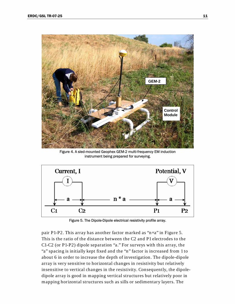
Figure 4. A sled-mounted Geophex GEM-2 multi-frequency EM induction
instrument being prepared for surveying.
Figure 5. The Dipole-Dipole electrical resistivity profile array.
pair P1-P2. This array has another factor marked as “n∗a” in Figure 5. This is the ratio of the distance between the C2 and P1 electrodes to the C1-C2 (or P1-P2) dipole separation “a.” For surveys with this array, the “a” spacing is initially kept fixed and the “n” factor is increased from 1 to about 6 in order to increase the depth of investigation. The dipole-dipole array is very sensitive to horizontal changes in resistivity but relatively insensitive to vertical changes in the resistivity. Consequently, the dipole-dipole array is good in mapping vertical structures but relatively poor in mapping horizontal structures such as sills or sedimentary layers. The
GEM-2
Control Module

ERDC/GSL TR-07-25 12
median depth of investigation of this array also depends on the “n” factor, as well as the “a” factor.
One possible disadvantage of this array is the very small signal strength for large values of the “n” factor. The voltage is inversely proportional to the cube of the “n” factor. This means that for the same current, the voltage measured by the resistivity meter drops by about 200 times when “n” is increased from 1 to 6. One method to overcome this problem is to increase the “a” spacing between the C1-C2 (and P1-P2) dipole pair to reduce the drop in the potential when the overall length of the array is increased to increase the depth of investigation.
A Scintrex Automated Resistivity Imaging System (SARIS) (Scintrex Ltd.) was used in this investigation (Figure 6). A resistivity cable providing the ability to connect to 25 electrodes was connected to the meter. An “a” spac-ing of 5 m and “n” factors of 1 through 6 were used to collect the data. A roll-along method was used to advance the profile line. The sequence of measurements, array type, and other survey parameters were entered into the SARIS resistivity meter. A program in the meter then automatically selected the appropriate electrodes for each measurement. The measure-ments were taken in a systematic manner and all possible measurements were made. At the end of the survey, the data were transferred to a com-puter for further processing.
Capacitively coupled conductivity surveys
An instrument using the CCR principle of operation was also used in this investigation to collect soil conductivity information. The CCR principle of operation is very similar to the dc resistivity method. Instead of using metal electrodes that have to be hammered into the ground as a means to inject current into the subsurface, as is the case in dc resistivity surveying, the CCR method capacitively injects the current into the ground. A trans-mitter electrifies two coaxial cables (transmitter dipole) with a 16.5-kHz alternating current (ac) signal. The dipole electrodes consist of coaxial cables in which the coaxial cable shield acts as one plate of a capacitor and the earth as the other plate. A matched receiver, automatically tuned to the transmitter frequency, measures the associated voltage picked up on the receiver’s dipole cables. The receiver then transmits a voltage measure-ment, normalized to current, to the logging console.

ERDC/GSL TR-07-25 13
Figure 6. SARIS dc electrical resistivity survey arrangement.
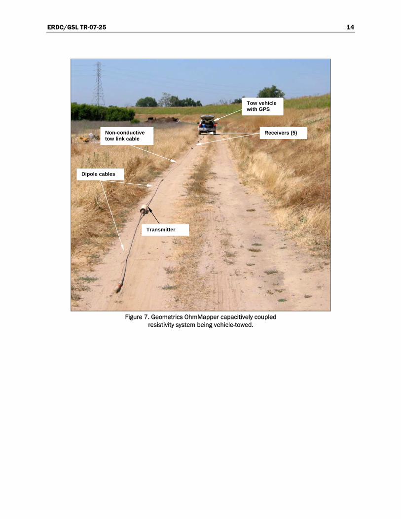
A Geometrics OhmMapper capacitively coupled resistivity system was used to collect the resistivity data. The system used in this investigation can use from one to five receivers allowing for multiple n-spacings to be collected per survey pass. Figure 7 shows the OhmMapper being used at the Feather River site with a five-receiver setup and being vehicle-towed. The “a” spacing or dipole length was 5 m and “n” factors of 3.0, 3.5, 4.0, 4.5, and 5.0 were used. Using this configuration the length of the array was in excess of 35 m. The OhmMapper was set to collect data once every sec-ond. Data positioning was achieved by means of a GPS. The data were col-lected at a slow walking pace of approximately 2 km/hr.
At the end of each survey, field data were transferred to a laptop computer for analysis. The data were analyzed using program MagMapper 2000 (Geometrics 2004) to ensure the proper geometry of the survey lines. MagMapper was also used to convert the resistivity data into a format compatible with the resistivity inversion program RES2DINV.
Steel electrodes
Multi-conductor cable
SARIS meter
Steel electrodes
Multi-conductor cable
SARIS meter
ERDC/GSL TR-07-25 14
Figure 7. Geometrics OhmMapper capacitively coupled
resistivity system being vehicle-towed.
Dipole cables
Non-conductive tow link cable
Receivers (5)
Tow vehicle with GPS
Transmitter
ERDC/GSL TR-07-25 15
3 Geophysical Test Results, Interpretation and General Discussion
Geophysical test results
EM31 and EM34 results
Data were collected in approximately 3 days using the EM31 and EM34. Because this was the first time this sled system had been used, consider-able part of this time was spent configuring it for the different EM34 Tx-Rx coil separations. The sled system worked well in this environment and no major problems were encountered while towing. Not having wheels on the sleds kept them from running into each other when the tow vehicle slowed down or stopped along the survey line. At some road crossings and when inaccessible areas were encountered, the sled system had to be dis-mantled, hauled to the next start location, and set up again.
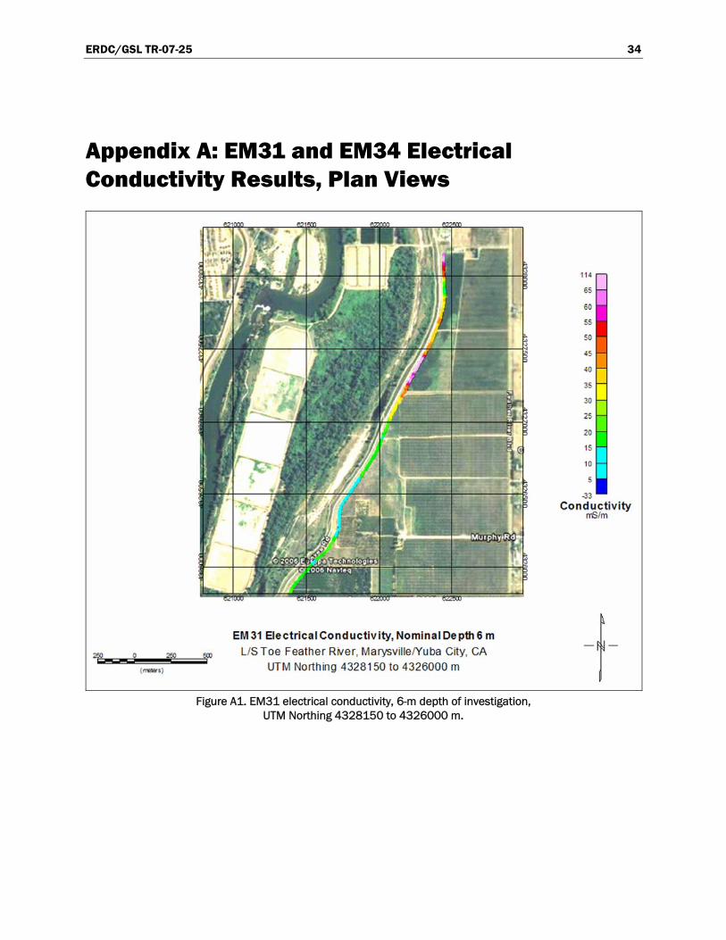
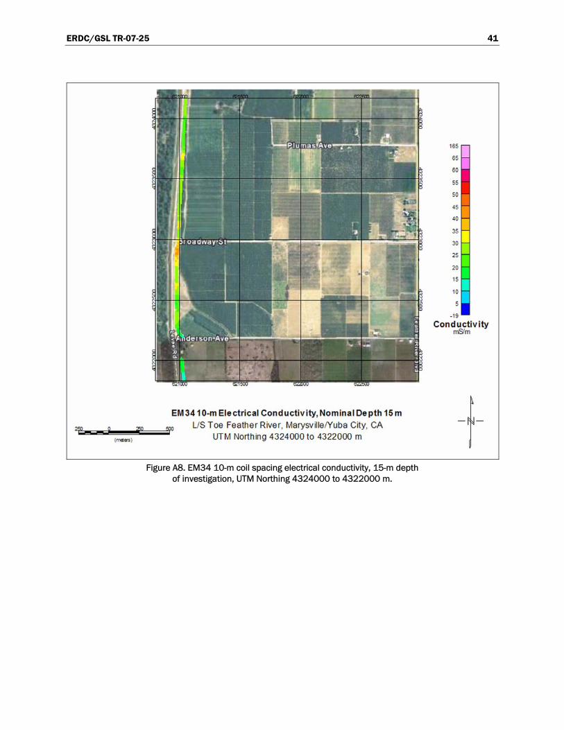
The EM31 and EM34 electrical conductivity results are presented together in three fashions: (a) plan view, (b) profile format, and (c) as a pseudo-section, shown in Appendix A, B, and C, respectively. The plan views (Appendix A, Figures A1–A20) show a color-coded representation of the subsurface electrical conductivity along the survey line. Plan views are pre-sented for the EM31 and EM34 (10-, 20-, and 40-m) data, which provide conductivity information for different depths of investigation. The plan views are superimposed on digital aerial images and provide a spatial sense of where anomalous conditions exist. Comparison of the different plan views for a given location shows how conductivity values vary as a function of depth (coil separation).
The profile plots (Appendix B, Figures B1–B18) show the electrical conductivity readings collected for the EM31, as well as for each EM34 intercoil configuration, versus Universal Transverse Mercator (UTM) nor-thing. With the exception of Figure B1, which covers a distance of 650 m, each figure covers a distance of 500 m.
The pseudosections (Appendix C, Figures C1–C18) present a two-dimensional (2-D) representation of the subsurface conductivity values. Data for apparent conductivity from the EM31 and EM34 are contoured on the assumption that the EM31 has a nominal depth of investigation of 3 m

ERDC/GSL TR-07-25 16
and that the EM34 intercoil spacings of 10, 20, and 40 m have nominal depths of investigation of 15, 30, and 60 m, respectively. The contoured values shown in the pseudosections are apparent conductivities and not true conductivities. Although the pseudosection may not present true con-ductivity values or accurately portray layering depth, they are useful in determining general trends and the locations of anomalous areas. To pro-duce an image of true depth and true formation conductivity, the observed data must be processed using an inversion algorithm.
In general, the EM data show that the greater the depth of investigation i.e., longer intercoil spacing, the greater the conductivity values. Table 2 shows average and median conductivity values increasing as a function of coil separation (depth). This indicates that there is a general trend of finer grained materials increasing with depth. Electrical conductivity is a posi-tive valued parameter; however, because of instrument design negative values are measured when passing over a metallic object.
Table 2. EM31 and EM34 statistical values.
Instrument and Intercoil Spacing
Average Conductivity, mS/m
Median Conductivity, mS/m
Minimum Conductivity, mS/m
Maximum Conductivity, mS/m
Standard Deviation
No. of Data Points
EM31 3.667 m 26 23 -81 121 14.7 44,373 EM34 10 m 31 26 -55 183 17.2 32,897 EM34 20 m 35 34 -27 194 16.6 28,465 EM34 40 m 47 43 -99 319 32.7 26,312
The plots shown in the appendixes use the same linear color bar scale, which allows for direct comparison of conductivity values for the different plot types. The red and pink colors are relatively high conductivity values associated with clayey soil, whereas the dark green and blue colors, low conductivity values, are indicative of a soil with a greater proportion of sands and gravels.
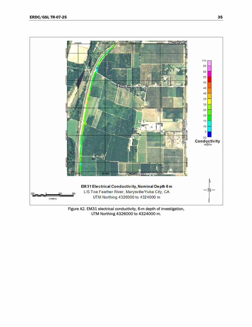
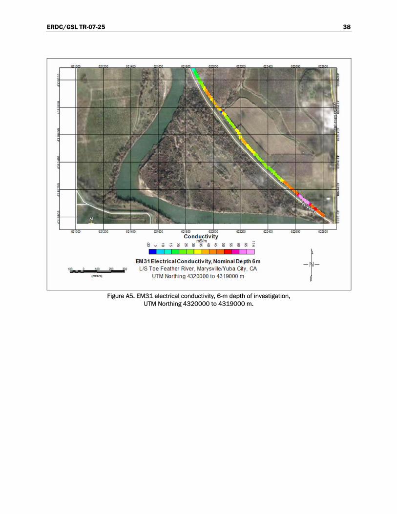
The EM31 data, which have a depth of investigation of approximately 6 m, show an area of relatively high conductivity materials at the northern end of the survey site (Figure A1). The data south of approximate Sta-tion 4327000 are generally green and blue in color, representative of materials that are predominantly sands and gravels (Figures A2–A4). At the extreme southern end of the survey line there is a pink-colored zone indicating a clayey area (Figure A5). The EM34 10-m data, Figures A6–A10, are in general the same or show slightly higher conductivity values

ERDC/GSL TR-07-25 17
than the EM31 data, indicating no significant material type differences between the upper 6 and 15 m. The 20- and 40-m plan view data show a slight general increase in conductivity values as compared to the EM31 and EM34 10-m data, indicating an increase in silt and/or clay between approximate depths of 30 and 60 m (Figures A11–A20). A predominant, relatively low, conductivity area indicated by the EM31, EM34 10-m and EM34 20-m data occurs from approximately Anderson Ave., Sta-tion 4322200, south to the approximate location of a water pumping plant near Station 4319775.
Referring to Figure B1, the conductivity values show some variability. Between Stations 4328150 and 4328100, there is an indication that the near surface materials (upper 15 m) are quite clayey compared with the near surface materials encountered along the rest of the survey line. Between Stations 4327950 and 4327850, the EM31 and the EM34 10-m profile lines show relatively low conductivity readings, indicating the pres-ence of a layer of coarse-grained materials in the upper 15 m. Of particular interest is the anomalous area between Stations 4327475 and 4327150 (Figure B2). There is a very significant positive-valued spiking of all the EM data. The EM31 and the EM34 10- and 20-m surveys show three dis-tinct spikes centered on Stations 4327400, 4327280, and 4327180, whereas the EM 34 40-m data show one very broad spike between Sta-tions 4327475 and 4327250 and a much smaller one centered at Sta-tion 4327180. The broad, relatively high conductivity spike is an indication of an increase in conductive (fine-grained) materials with depth. This may be caused by a clay-filled abandoned channel. The area between approxi-mate Stations 4327900 and 4327250 show higher conductivity values (more fine-grained material) in comparison to the rest of the survey line. Between approximate Stations 4327000 and 4322800, the readings for the EM31 and the three EM34 spacings are fairly consistent with some localized fluctuations (Figures B3–B11). Along this stretch, the EM31 and the EM34 10-m readings range roughly between 10 and 30 mS/m, the EM34 20-m readings range between approximately 35 and 40 mS/m, and the EM34 40-m readings range between approximately 40 and 50 mS/m.
Between approximate Stations 4322800 and 4320000 (Figures B11 and B16), the conductivity values show a general decline. In this area, the EM31 and the EM34 10-m readings range roughly between 10 and 20 mS/m, the EM34 20-m readings range between approximately 20 and 30 mS/m and the EM34 40-m readings range between
ERDC/GSL TR-07-25 18
approximately 30 and 40 mS/m. This area exhibited the lowest conductiv-ity values of the entire survey line. It is presumed that this is an area with extensive sands and gravels.
Between approximate Stations 4320000 and 4319000 (Figures B17 and B18), the conductivity values for the EM31 and the EM34 10- and 20-m readings show a general increase. The EM34 40-m conductivity values in this area are about the same as the previous area to the north. It appears that fine-grained materials in the upper 20 m may be increasing in this area. The conductivity values of the deeper materials interrogated by the EM34 40-m test show values of about 40 mS/m, which are higher than the previous area to the north but not as high as the northern portion of the survey line.
GEM-2 results
User-selected GEM-2 frequencies for this survey were 9810, 6390, 1590, and 390 Hz and were chosen to correspond with the EM31 (9800-Hz), EM34 10-m (6400-Hz), 20-m (1600-Hz), and 40-m (400-Hz) intercoil spacings, respectively. It took approximately 1 day to collect the GEM-2 data. The GEM-2 results are plotted in profile fashion and to the same scale as the EM31 and EM34 plots to aid in comparing the results of the three different instruments (Appendix D). The GEM-2 390-Hz data are not shown because the data were too noisy. The 9810- and 6390-Hz data are almost identical with the main difference between the two frequencies being that the 9810-Hz data are consistently about 1 to 2 mS/m less than the 6390-Hz data. The 1590-Hz GEM-2 data do not appear to realistically represent the conductivities of the subsurface materials but they do respond very well to nearby metallic features. The GEM-2 9810-Hz and 6390-Hz profile data closely match the EM31 and EM34 10-m data. Table 3 presents some selected statistical values for the four GEM-2 frequencies. The table shows that the median values for the 9810-Hz and 6390-Hz data compare favorably with the EM31 and EM34 10-m median values.
The GEM-2 survey was run to obtain conductivity versus depth data and to compare with the EM31 and EM34 data. Unfortunately, because the 1590-Hz and the 390-Hz data are considered to be unreliable and the difference between the 9810- and 1590-Hz data generally varies by only

ERDC/GSL TR-07-25 19
Table 3. GEM-2 statistical values.
Frequency, Hz
Average Conductivity, mS/m
Median Conductivity, mS/m
Minimum Conductivity, mS/m
Maximum Conductivity, mS/m
Standard Deviation
No. of Data Points
9810 35 25 0 266 39.4 47,4016390 41 27 0 360 54.1 47,4011590 52 2 0 4020 172.1 47,401390 474 228 0 52,200 935.6 47,401
1 to 2 mS/m, the relationship of changes in soil type as a function of depth cannot be determined. Because the only two GEM-2 frequencies that appear to have realistic results are the 9810- and 1590-Hz data, the most similar frequencies to the EM31 and EM34 10-m spacing, it would be rea-sonable to assume that the GEM-2 data are providing conductivity values for the upper 5 to 15 m of material.
The GEM-2 data show relatively elevated conductivity values ranging gen-erally between 30 and 100 mS/m between approximate Stations 4328100 and 4327000 (Figures D1 and D2). There is one exception to these high conductivity values occurring at approximate Station 4327900 where there is an anomalously low conductivity area with an approximate conductivity range of 10 to 15 mS/m. With the exception of the anomalously low conductivity area, one should expect a relatively high proportion of silty and/or clayey material in the upper 5 to 15 m between Stations 4328100 and 4327000. Between approximate Stations 4327000 and 4326600 (Fig-ures D2 and D3), conductivity values are fairly consistent with values ranging between 15 and 20 mS/m, indicating the presence of rather coarse materials. Between approximate Stations 4326600 and 4326250, it is pre-sumed that the percentage of sands and gravels in the upper 5 to 15 m increases because the conductivity values drop to about 5 to 10 mS/m (Figures D3 and D4). Conductivity values between approximate Sta-tions 4326250 and 4324500 generally have values between 20 and 30 mS/m (Figures D4–D7). In this section, there are some areas where conductivity values exceed 30 mS/m, but only for relatively short dis-tances. Between approximate Stations 4326050 and 4325700, there are numerous large spikes that are presumably caused by metallic debris visi-ble on the ground surface (Figures D4 and D5). The large spikes observed at approximate Stations 4325275, 4325115, 4325075, and 432500 are probably caused by buried metallic irrigation pipes (Figure D6). The spike at Station 4325170 is caused by a vertical 1.2-m- diam corrugated steel standpipe located about 2 to 3 m west of the survey line. Another area with

ERDC/GSL TR-07-25 20
relatively large spiking values is encountered between Stations 4324125 and 4324300, and it is an area where there are many visible trash piles adjacent to the survey line (Figure D8). South of Station 4324300 to about Station 4323100 conductivity values range roughly between 10 and 20 mS/m (Figures D9 and D10). Between Stations 4323100 and 4322950, just to the north of Broadway Road, there is an area with fairly high conductivity values of about 80 mS/m (Figures D10 and D11). South of this area, a relatively high conductivity area to Anderson Avenue, Sta-tion 4322200, conductivity values range between approximately 20 and 30 mS/m (Figures D11 and D12). With the exception of an area between Stations 4321750 and 4321650 with conductivity values of about 25 mS/m, the area between 4322000 and 4321500 has relatively low conductivity values ranging between approximately 5 and 15 mS/m, indicative of sandy and/or gravelly material (Figure D13). The conductivity values encoun-tered in this area are some of the lowest for the entire survey line. Another area with relatively low conductivity values ranging between 10 and 20 mS/m is found between Stations 4321050 and 4320000 (Figures D14–D16). Between Station 4320000 and the south end of the survey line, con-ductivity values are significantly higher generally ranging between 20 and 40 mS/m (Figures D17 and D18).
OhmMapper results
The results of the OhmMapper CCR survey are shown in Appendix E (Fig-ures E1–E18). The data are presented as a 2-D cross section with northing shown along the X-axis and depth along the Y-axis. In these cross sections, the contoured values represent the true electrical conductivity. The OhmMapper transmitter-receiver distances used in this investigation pro-vided conductivity information for depths between approximately 1 and 11 m. Whereas the EM data provide a greater depth of information at the expense of being able to resolve relatively small subsurface features, the OhmMapper provides detailed conductivity information in the upper 11 m, thus complementing the EM data. Even with an array in excess of 35 m in length, the array tracked well behind the tow vehicle. The shallow ruts in the unpaved levee-toe road appear to have helped keep the array on track especially around curves.
The OhmMapper data compare favorably with the results of the EM data. Between approximate Stations 4328000 and 4326950, there is a fairly thin, approximately 5-m thick, layer with low conductivity values overlying a much higher conductivity valued layer (Figures E1–E3). This is the same

ERDC/GSL TR-07-25 21
area where relatively high conductivity values are detected with the EM instruments. Between approximate Stations 4326950 and 4323150, the materials in the upper 5 to 10 m generally have conductivity values that increase with depth and range between approximately 5 and 25 mS/m (Figures E3–E10). In this area, zones of higher conductivity materials are detected at depths greater than 10 m. Between approximate Sta-tions 4326600 and 4326450, the true conductivity values in the upper 11 m are extremely low and do not exceed 5 mS/m (Figures E3 and E4). These low conductivity values are indicative of loose sandy and/or gravelly material. Between approximate Stations 4323150 and 4322600, the conductivity values in the upper 11 m appear to increase slightly, suggest-ing an increase in fine-grained material in this area (Figures E10 and E11). With the exception of an area between Station 4321800 and 4321700, the area between approximate Stations 4322550 and 4320000 generally exhibits rather low true conductivity values of less than 25 mS/m (Figures E11–E16). Conductivity values tend to increase south of Station 4320000, indicating an increase in fine grained soil.
SARIS results
A 1055-m-long dc electrical resistivity line was run near the northern end of the site between approximate Stations 4327744 and 4326795. Inversion results provide conductivity information between approximate depths of 1 and 8.5 m. The dc resistivity survey method is the slowest and most labor intensive of all of the survey methods used in this investigation; however, it provides very detailed lateral and vertical material information. The approximate 1-km-long dc resistivity line took about 1 day to collect. An inspection of the data showed considerable noise that is presumed to be caused by the high contact resistance between the ground and the resistiv-ity electrodes. The data points considered to be “bad” were removed prior to processing.
The dc resistivity results are shown in Appendix F (Figures F1–F3). Between approximate Stations 4327700 and 4327450, the conductivity values are less than 25 mS/m in the upper 2 to 3 m and are underlain by more conductive (clayey) materials (Figures F1 and F2). However, between Stations 4327450 and 4327200 (Figure F2), the conductivity values are greater than 50 mS/m in the upper 2 m and are underlain by less conduc-tive materials. Further to the south along the survey line, between approxi-mate Stations 4327000 and 4326800 (Figure F3), the conductivity values

ERDC/GSL TR-07-25 22
are generally less than 10 mS/m, indicative of dry sandy soil in the upper 8.5 m.
Interpretation of results
The results of the EM, OhmMapper, and dc resistivity surveys, in general, agree very well. Soil distribution maps for the survey site were created based on an interpretation of the geophysical data (Figures 8 through 10). Six soil classes were used to create the maps; sand/gravel (<10 mS/m), sand (10–19 mS/m), silt/sand (20–34 mS/m), silt (35–49 mS/m), silt/clay (50–59 mS/m), and clay (>59 mS/m). The site can be generally be characterized as consisting of sands and gravels from the surface to depths of approximately 5 to 15 m underlain by silt/sand and silt to depths of approximately 40 to 50 m, which in turn are underlain by silt/clay.
The survey results also indicate seven anomalous zones (Table 4). Anomalous Zone I extends from the north end of the survey line, Station 4328000, south to approximate Station 4327450 (Figure 8). Anomalous Zone I is an area with a thinning, or an absence, of low conductivity soil in the near surface which is replaced with predominantly higher conductivity soil. Nearby borings indicate the presence of shallow, thick clay lenses and/or layers. These clays are the probable cause for the higher conductivity values found in Zone I.
Interpreted Soils MapL/S Toe Feather River, Marysville/Yuba City, CA
UTM 4328000 to 4325000
Sand/Gravel
Sand
Silt/Sand
Silt
Silt/Clay
Clay
Dep
th, m
Zone I Zone II Zone IIIAnomalousAnomalous Anomalous Anomalous
Zone IV
-60
-40
-20
0-60
-40
-20
0
-4328000 -4327500 -4327000 -4326500 -4326000 -4325500 -4325000
-4328000 -4327500 -4327000 -4326500 -4326000 -4325500 -4325000
Figure 8. Interpreted soil distribution map, UTM 4328000 to 4325000.
ERDC/GSL TR-07-25 23
Interpreted Soils MapL/S Toe Feather River, Marysville/Yuba City, CA
UTM 4325000 to 4322000
Sand/Gravel
Sand
Silt/Sand
Silt
Silt/Clay
Clay
Dept
h, m
-60
-40
-20
0-60
-40
-20
0
-4325000 -4324500 -4324000 -4323500 -4323000 -4322500 -4322000
-4325000 -4324500 -4324000 -4323500 -4323000 -4322500 -4322000
AnomalousZone V
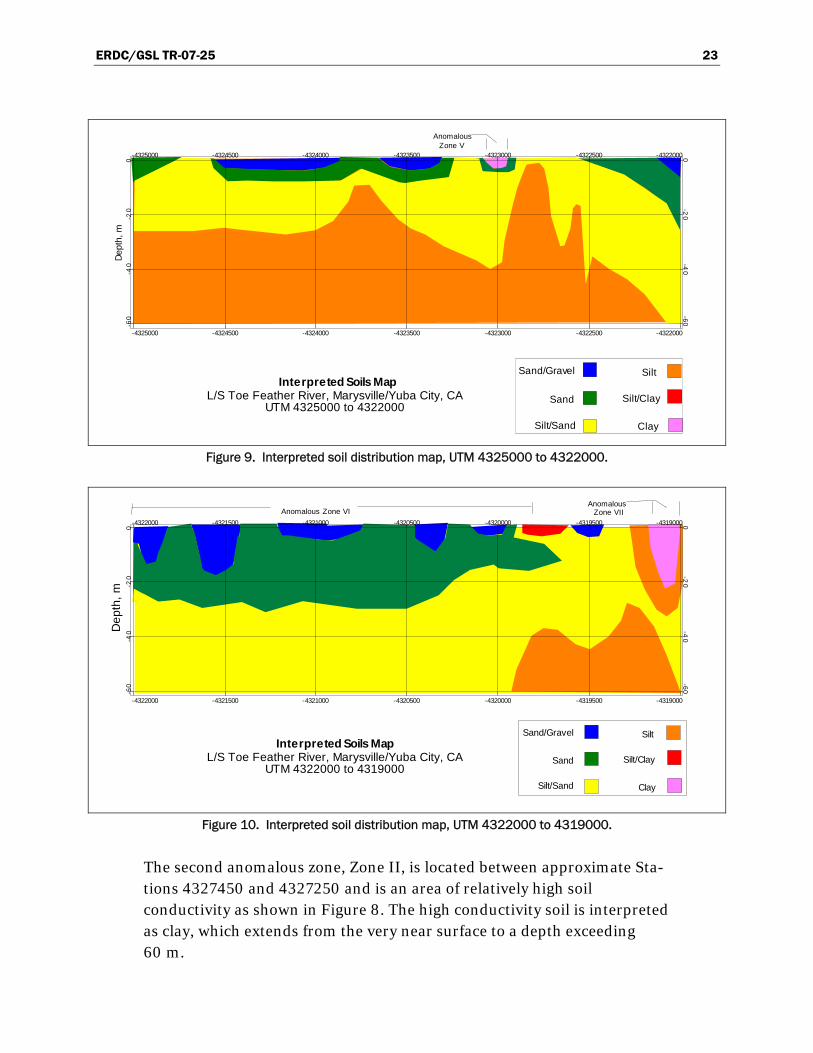
Figure 9. Interpreted soil distribution map, UTM 4325000 to 4322000.
Interpreted Soils MapL/S Toe Feather River, Marysville/Yuba City, CA
UTM 4322000 to 4319000
Sand/Gravel
Sand
Silt/Sand
Silt
Silt/Clay
Clay
Dep
th, m
-60
-40
-20
0-60
-40
-20
0
-4322000 -4321500 -4321000 -4320500 -4320000 -4319500 -4319000
-4322000 -4321500 -4321000 -4320500 -4320000 -4319500 -4319000Anomalous Zone VI
Anomalous Zone VII
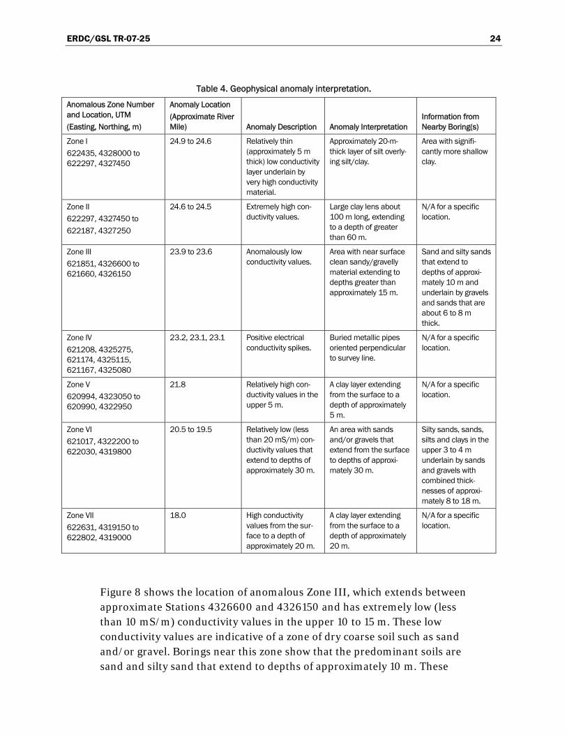
Figure 10. Interpreted soil distribution map, UTM 4322000 to 4319000.
The second anomalous zone, Zone II, is located between approximate Sta-tions 4327450 and 4327250 and is an area of relatively high soil conductivity as shown in Figure 8. The high conductivity soil is interpreted as clay, which extends from the very near surface to a depth exceeding 60 m.
ERDC/GSL TR-07-25 24
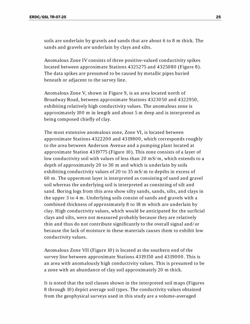
Table 4. Geophysical anomaly interpretation.
Anomalous Zone Number and Location, UTM (Easting, Northing, m)
Anomaly Location (Approximate River Mile) Anomaly Description Anomaly Interpretation
Information from Nearby Boring(s)
Zone I 622435, 4328000 to 622297, 4327450
24.9 to 24.6 Relatively thin (approximately 5 m thick) low conductivity layer underlain by very high conductivity material.
Approximately 20-m-thick layer of silt overly-ing silt/clay.
Area with signifi-cantly more shallow clay.
Zone II 622297, 4327450 to 622187, 4327250
24.6 to 24.5 Extremely high con-ductivity values.
Large clay lens about 100 m long, extending to a depth of greater than 60 m.
N/A for a specific location.
Zone III 621851, 4326600 to 621660, 4326150
23.9 to 23.6 Anomalously low conductivity values.
Area with near surface clean sandy/gravelly material extending to depths greater than approximately 15 m.
Sand and silty sands that extend to depths of approxi-mately 10 m and underlain by gravels and sands that are about 6 to 8 m thick.
Zone IV 621208, 4325275, 621174, 4325115, 621167, 4325080
23.2, 23.1, 23.1
Positive electrical conductivity spikes.
Buried metallic pipes oriented perpendicular to survey line.
N/A for a specific location.
Zone V 620994, 4323050 to 620990, 4322950
21.8 Relatively high con-ductivity values in the upper 5 m.
A clay layer extending from the surface to a depth of approximately 5 m.
N/A for a specific location.
Zone VI 621017, 4322200 to 622030, 4319800
20.5 to 19.5 Relatively low (less than 20 mS/m) con-ductivity values that extend to depths of approximately 30 m.
An area with sands and/or gravels that extend from the surface to depths of approxi-mately 30 m.
Silty sands, sands, silts and clays in the upper 3 to 4 m underlain by sands and gravels with combined thick-nesses of approxi-mately 8 to 18 m.
Zone VII 622631, 4319150 to 622802, 4319000
18.0 High conductivity values from the sur-face to a depth of approximately 20 m.
A clay layer extending from the surface to a depth of approximately 20 m.
N/A for a specific location.
Figure 8 shows the location of anomalous Zone III, which extends between approximate Stations 4326600 and 4326150 and has extremely low (less than 10 mS/m) conductivity values in the upper 10 to 15 m. These low conductivity values are indicative of a zone of dry coarse soil such as sand and/or gravel. Borings near this zone show that the predominant soils are sand and silty sand that extend to depths of approximately 10 m. These
ERDC/GSL TR-07-25 25
soils are underlain by gravels and sands that are about 6 to 8 m thick. The sands and gravels are underlain by clays and silts.
Anomalous Zone IV consists of three positive-valued conductivity spikes located between approximate Stations 4325275 and 4325080 (Figure 8). The data spikes are presumed to be caused by metallic pipes buried beneath or adjacent to the survey line.
Anomalous Zone V, shown in Figure 9, is an area located north of Broadway Road, between approximate Stations 4323050 and 4322950, exhibiting relatively high conductivity values. The anomalous zone is approximately 100 m in length and about 5 m deep and is interpreted as being composed chiefly of clay.
The most extensive anomalous zone, Zone VI, is located between approximate Stations 4322200 and 4319800, which corresponds roughly to the area between Anderson Avenue and a pumping plant located at approximate Station 4319775 (Figure 10). This zone consists of a layer of low conductivity soil with values of less than 20 mS/m, which extends to a depth of approximately 20 to 30 m and which is underlain by soils exhibiting conductivity values of 20 to 35 mS/m to depths in excess of 60 m. The uppermost layer is interpreted as consisting of sand and gravel soil whereas the underlying soil is interpreted as consisting of silt and sand. Boring logs from this area show silty sands, sands, silts, and clays in the upper 3 to 4 m. Underlying soils consist of sands and gravels with a combined thickness of approximately 8 to 18 m which are underlain by clay. High conductivity values, which would be anticipated for the surficial clays and silts, were not measured probably because they are relatively thin and thus do not contribute significantly to the overall signal and/or because the lack of moisture in these materials causes them to exhibit low conductivity values.
Anomalous Zone VII (Figure 10) is located at the southern end of the survey line between approximate Stations 4319150 and 4319000. This is an area with anomalously high conductivity values. This is presumed to be a zone with an abundance of clay soil approximately 20 m thick.
It is noted that the soil classes shown in the interpreted soil maps (Figures 8 through 10) depict average soil types. The conductivity values obtained from the geophysical surveys used in this study are a volume-averaged

ERDC/GSL TR-07-25 26
conductivity. For example, the area under the survey line may consist predominantly of sand with interbedded thin clay and silt layers. Because the volume of the clay and/or silt is much less than that of the host sand, the clay and silt layers make a small contribution to the measured conductivity values. The surveyed area exhibits low conductivity values and is interpreted as sand. As the amount of silt and clay increases, the conductivity values correspondingly increase and the soil class would then be interpreted as one with greater fines, i.e., silt/sand. Also, the greater the depth of investigation for a geophysical instrument the greater is the volume of soil being measured. This means that, as the depth of investigation increases, the ability to resolve relatively small features decreases. Conversely, small features can be more easily resolved at relatively shallower depths of investigation. This explains why relatively small features are interpreted only in the near-surface in Figures 8–10.
General discussion
The Geonics EM and the OhmMapper instruments are considered the most useful in characterizing this site (Feather River, Marysville/Yuba City, CA) because of their ability to provide electrical conductivity data for various depths and rapid data acquisition rate. The dc electrical resistivity provides very detailed information between depths of approximately 1 and 8 m; however, the slow data collection rate, as compared with the EM and CCR surveys, and high contact resistance problems make this a secondary survey method for this site. It is noted that all the surveys were conducted using a two-person field crew. An increase by one or two field personnel would significantly increase the rate at which dc resistivity readings could be collected and slightly increase the EM and CCR data collection rate.
In this investigation the EM34 was used with the coils parallel to the ground surface (vertical dipole) using three intercoil spacings, thus provid-ing conductivity information at estimated depths of 15, 30, and 60 m. By configuring the coils perpendicular to the ground surface and coplanar, horizontal dipole data could be collected for three additional depths. The depth of exploration is 0.75 times the intercoil distance when the EM34 is used in the horizontal dipole mode (McNeil 1980). This would allow con-ductivity values for three additional depths, for a given location, to be input into an inversion program. The inversion program could then output true electrical conductivity values and layer depths, thus allowing conduc-tivity depth sections to be plotted. Similarly, the EM31 can also be used with horizontal dipoles simply by rotating it 90 deg about its long axis. The

ERDC/GSL TR-07-25 27
combination of the EM31 and EM34 used in horizontal and vertical dipole modes can provide eight conductivity values per location, which would improve the inversion results.
The OhmMapper CCR instrument proved to be very effective in mapping soil conductivity values. The instrument, as configured in this survey, pro-vided conductivity data between depths of approximately 1 and 11 m. The five-receiver version of the OhmMapper used in this investigation made it possible to collect sufficient data in one survey pass to produce conductiv-ity depth sections. The software provided with the OhmMapper was used to convert the collected data into a format compatible with the inversion program RES2DINV. The very low conductivity soils encountered at this site were ideal field conditions for the OhmMapper. The 35-m-long array used in this survey tracked well behind the tow vehicle along the slightly rutted unpaved levee-toe road. The tire ruts in the sandy road acted as a guide for the instrument array.
The GEM-2 did not perform well. It was hoped that the GEM-2 would provide enough information to make it possible to perform an inversion of the data. Only two of four programmed frequencies, 6390 and 9810 Hz, were regarded of any use, and they showed nearly identical results. No conclusions on how soil conductivity varied as a function of depth could be made from the values collected with this instrument. Information from only two frequencies is not sufficient to perform an inversion of the data. However, the GEM-2 is useful for mapping lateral conductivity differences. The data from the other two frequencies used, 1590 and 390 Hz, were noisy and unusable. It is not known whether these frequencies are beyond the instrument’s capabilities for this site or whether lack of experience in using the GEM-2 by the field researchers may have contributed to the collection of poor data.
This study shows that geophysical surveys are useful for rapidly mapping long reaches of levees. This site was particularly amenable to the geophysical methods used because of good site access, no vehicular traffic, minimal interference from cultural features, and low electrical conductivity soils. It is important to have good access to the levee toe for long uninterrupted stretches to prevent data gaps, make interpretation of test results easier, and minimize the time to break down and set up equipment when circumventing obstacles along a survey line. EM geo-physical survey methods, such as used in this study, are prone to

ERDC/GSL TR-07-25 28
interference from nearby metallic objects (such as buildings, cars, and culverts) and power lines; this interference is referred to as cultural clutter. Survey lines that run through areas with large amounts of cultural clutter, such as found in a highly urbanized environment, may prove to be problematic for EM methods. In such cases, other methods that are less susceptible to cultural clutter may have to be used. These include dc resistivity, CCR, and seismic surveying methods.
The EM34 conductivity meter is the instrument that has the greatest depth of investigation potential. At sites having ideal soil conditions (soil conductivity values less than 10 mS/m) the EM34 has a depth of investigation of approximately 60 m. However, as soil conductivity values increase, the depth of investigation decreases.
Geophysical data can be arranged, by conductivity value, into different classes or ranges that, when correlated to nearby borings, can be used as a means to classify soil. By examining the EM pseudosections and electrical conductivity plots, presented in the appendixes, geotechnical engineers and geologists can visualize the lateral and vertical extent of the different soil types at the site.
Also, during this study, an emergency management exercise was conducted. As part of the exercise, geophysical data were collected along the levee toe during a simulated flooding event, electronically uploaded from the field to the USACE’s Integrated Levee Assessment Utility Web site, and saved in a database. The data were tabulated and made accessible in near real-time via the Web to emergency operations personnel. Anomalies along the survey line, suggesting areas of sands and gravels, which are prone to under-seepage, were quickly identified. The exercise showed that providing access to near real-time data, regarding levees and levee foundation conditions, to emergency operations personnel can allow for enhanced situational awareness during times of crisis. Figure 11 shows an example of the type of data available from the USACE Web site.

ERDC/GSL TR-07-25 29
Figure 11. Example of a portion of EM34 data plot posted on the Integrated Levee
Assessment Utility Web site.
ERDC/GSL TR-07-25 30
4 Conclusions and Recommendations Conclusions
Geophysical surveys were conducted along the Feather River levee approximately 5 km south of Marysville/Yuba City, CA, during the period 14–21 June 2006. The purpose of this study was to determine the potential of rapidly assessing levee foundations using geophysical methods. The study was funded by the USACE’s Emergency Management Technologies focus area of the FCSDR research program.
The test site was located on the landside toe of the levee on the east side of the Feather River. The survey site extended south from the water treat-ment plant located approximately 2 km south of Island Avenue, to just north of the Star Bend boat ramp. The approximate northern and southern UTM coordinates, in meters, of the survey site are 622435, 4328000 and 622802, 4319000, respectively. The north and south ends of the survey line correspond to approximate USACE Sta. 434+00 and Sta. 106+00, respectively. The north and south ends of the survey line correspond to approximate RM 24.9 and 18.0, respectively. The site is located within Reclamation District 784. The materials underlying the site are alluvial in nature and consist of clay, silt, sand, and gravel.
Three geophysical survey methods were used to collect soil conductivity information: electromagnetic (EM) induction, capacitively coupled elec-trical resistivity, and direct current electrical resistivity. Boring logs from nearby borings were used to correlate soil type with soil electrical conduc-tivity values. Soil conductivity maps were generated and used to infer soil type and anomalous conditions to depths of approximately 60 m along the 10-km-long survey line. Geophysical data to sufficiently characterize this site can be collected in approximately 1 day.
The combination of the geophysical instruments used in this survey pro-vided useful data, which were used to assess soil type along the survey line. The interpreted survey data indicate that, in general, the site consists of dry silty sandy material from the surface to approximately 10 m in depth. These soils are interpreted to be underlain by material that is more clayey in nature. Seven zones with anomalous survey results were interpreted. The first anomalous zone (Zone I), which extends from the north end of

ERDC/GSL TR-07-25 31
the survey line (UTM coordinate 622435, 4328000) south to approximate UTM coordinate 622297, 4327450, consists of a 20-m-thick layer of silt overlying soil materials with a higher clay content. Anomalous Zone II (located between coordinates 622297, 4327450 and 622187, 4327250) is interpreted as an extensive clay lens that is approximately 100 m long and 60 m deep. The third zone (Zone III) extends between approximate UTM coordinates 621851, 4326600 and 621660, 4326150. The soils in this area are interpreted as consisting chiefly of sands and/or gravels in the upper 10 to 15 m and underlain by clays. The fourth anomalous zone (Zone IV) extends between UTM coordinates 621208, 4322200 and 621167, 4325080. There are numerous positive-valued electrical conductivity spikes within this zone, presumably caused by buried metallic pipes. Anomalous Zone V (located between approximate coordinates 620994, 4323050 and 620990, 4322950) is composed chiefly of clay soil that extends from the surface to a depth of approximately 5 m. Anomalous Zone VI is located between approximate coordinates 621017, 4322200 and 622030, 4319800 or roughly the area between Anderson Avenue and south to Pump Station No. 3. This anomalous zone indicates a high proportion of sands and gravels from the surface to depths in excess of 30 m. This is an area where the levee failed in 1997. Anomalous Zone VII is located at the southern end of the survey line between approximate coordinates 622631, 4319150 and 622802, 4319000. This anomalous zone is presumed to consist of clay soil approximately 20 m thick. The geophysical interpretations were compared with nearby borings, which were mainly located along the crest of the levee, and showed very good agreement.
Two Geonics Ltd. EM conductivity meters (Geonics EM31 and EM34 conductivity meters), a Geometrics OhmMapper CCR system, a Geophex GEM-2 EM induction tool, and a Scintrex dc resistivity system were used to collect electrical conductivity data. The use of a vehicle-towed sled-mounted EM34 using three different intercoil spacings and the ability to collect continuous data made it possible to rapidly collect information at different depths of investigation. This allowed inferences about material type changes to be made laterally, as well as vertically. Estimated depths of exploration for the EM31 and the EM34 10-, 20-, and 40-m intercoil spacings are 6, 15, 30, and 60 m, respectively.
The OhmMapper CCR system provided detailed depth and electrical con-ductivity information between depths of 1 and 11 m for this site. Although

ERDC/GSL TR-07-25 32
the OhmMapper may have a depth of exploration less than that of the EM34, the five-receiver model used in this investigation has the advantage of being able to collect sufficient data in one survey pass to rapidly produce a conductivity depth section using a commercial resistivity inversion program.
Data collection problems encountered with the Geophex GEM-2 EM instrument prevented an inversion of the data to be performed. Only two of four programmed frequencies were considered useful, and they showed nearly identical results. The GEM-2 data were useful in determining lat-eral but not vertical soil variability. The depth of investigation for the GEM-2 is unknown.
Recommendations
Based on the results of this investigation, the following recommendations are made:
1. Conduct further studies using the Geonics EM31 and EM34 with horizon-tal and vertical dipole configurations. This should provide sufficient data for use in an inversion program.
2. Modify the EM34, making it possible to obtain data from the three differ-ent intercoil distances and both dipole configurations in one survey pass.
3. Identify commercial off-the-shelf inversion programs or take steps to develop a computer program that can quickly invert EM31 and EM34 data.
4. Identify sources of alternative ground-based multi-coil frequency-domain EM induction systems for testing.
5. Perform further studies using the Geophex GEM-2 EM induction instru-ment to determine depth of exploration capabilities and to provide resis-tivity depth sections.
6. Georeference all soil borings within a survey area. Much of the boring information that exists is referenced to stationing, river miles, or to a reclamation district’s levee mile designation, making it difficult to compare the geophysical data to the boring data.

ERDC/GSL TR-07-25 33
References Bookman-Edmonston Engineering, Inc. 2006. Geotechnical evaluation report for Feather
River Slurry Wall Pump Station No. 3 Area. Rancho Cordova, CA.
Dunbar, J. B., R. F. Ballard, W. L. Murphy, T. E. McGill, J. L. Llopis, L. D. Peyman-Dove, and M. J. Bishop. (2003). Condition assessment of the U.S. International Boundary and Water Commission, Lower Rio Grande Valley levees, south Texas. Vol I, Main Text and Appendices. ERDC TR-03-4. Vicksburg, MS: U.S. Army Engineer Research and Development Center.
Geometrics (2004). MagMap 2000 (computer program). http://www.geometrics.com.
Hess, J. R., and G. L. Sills. 2004. A review of Corps of Engineers levee seepage practices in the Central California flood control system. In Working Rivers—Balanced Resource Management, Proceedings, 24th Annual USSD Conference, April 2004. St. Louis, MO.
Huang, H. 2005. Depth of investigation for small broadband electromagnetic sensors. Geophysics 70(6):G135-G142.
Keller, G. V., and F. C. Frischknecht. 1966. Electrical methods in geophysical prospecting. Oxford: Pergamon Press.
Locke, M. H. 2000a. Electrical imaging surveys for environmental and engineering studies. Lecture notes. http://www.geoelectrical.com/.
____. 2000b. RES2DINV, Rapid 2D resistivity and IP inversion (computer program). Concord, Ontario, Canada: IDS Scintrex.
Marchand, D. E., and A. Allwardt. 1981. Late Cenozoic stratigraphic units, northeastern San Joaquin Valley, California. Bulletin 1470. Reston, VA: U.S. Geological Survey.
McNeil, J. D. 1980. Electromagnetic terrain conductivity at low induction numbers. Technical Note TN-6. Mississauga, Ontario, Canada: Geonics Ltd.
Reid, R. L. 2005. Is California next? Civil Engineering 75(11), 39-47, 84-85.
U.S. Army Corps of Engineers. 2006. Geomorphic assessment of project alternatives for Feather River levee improvement between the Bear and Yuba Rivers. Sacramento, CA: USACE District, Sacramento.
Won, I. J. 2003 Small frequency-domain electromagnetic induction sensors. How in the
world does a small broadband EMI sensor with little or no source-receiver separation work? The Leading Edge (Apr):320-322.
ERDC/GSL TR-07-25 34
Appendix A: EM31 and EM34 Electrical Conductivity Results, Plan Views
Figure A1. EM31 electrical conductivity, 6-m depth of investigation,
UTM Northing 4328150 to 4326000 m.
ERDC/GSL TR-07-25 35
Figure A2. EM31 electrical conductivity, 6-m depth of investigation,
UTM Northing 4326000 to 4324000 m.

ERDC/GSL TR-07-25 36
Figure A3. EM31 electrical conductivity, 6-m depth of investigation,
UTM Northing 4324000 to 4322000 m.

ERDC/GSL TR-07-25 37
Figure A4. EM31 electrical conductivity, 6-m depth of investigation,
UTM Northing 4322000 to 4320000 m.
ERDC/GSL TR-07-25 38
Figure A5. EM31 electrical conductivity, 6-m depth of investigation,
UTM Northing 4320000 to 4319000 m.

ERDC/GSL TR-07-25 39
Figure A6. EM34 10-m coil spacing electrical conductivity, 15-m depth
of investigation, UTM Northing 4328150 to 4326000 m.

ERDC/GSL TR-07-25 40
Figure A7. EM34 10-m coil spacing electrical conductivity, 15-m depth
of investigation, UTM Northing 4326000 to 4324000 m.
ERDC/GSL TR-07-25 41
Figure A8. EM34 10-m coil spacing electrical conductivity, 15-m depth
of investigation, UTM Northing 4324000 to 4322000 m.

ERDC/GSL TR-07-25 42
Figure A9. EM34 10-m coil spacing electrical conductivity, 15-m depth
of investigation, UTM Northing 4322000 to 4320000 m.
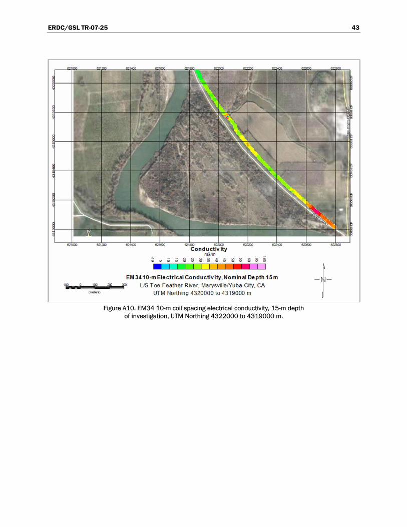
ERDC/GSL TR-07-25 43
Figure A10. EM34 10-m coil spacing electrical conductivity, 15-m depth
of investigation, UTM Northing 4322000 to 4319000 m.

ERDC/GSL TR-07-25 44
Figure A11. EM34 20-m coil spacing electrical conductivity, 30-m depth
of investigation, UTM Northing 4328150 to 4326000 m.

ERDC/GSL TR-07-25 45
Figure A12. EM34 20-m coil spacing electrical conductivity, 30-m depth
of investigation, UTM Northing 4326000 to 4324000 m.

ERDC/GSL TR-07-25 46
Figure A13. EM34 20-m coil spacing electrical conductivity, 30-m depth
of investigation, UTM Northing 4324000 to 4322000 m.
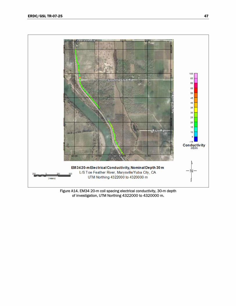
ERDC/GSL TR-07-25 47
Figure A14. EM34 20-m coil spacing electrical conductivity, 30-m depth
of investigation, UTM Northing 4322000 to 4320000 m.

ERDC/GSL TR-07-25 48
Figure A15. EM34 20-m coil spacing electrical conductivity, 30-m depth
of investigation, UTM Northing 4324000 to 4322000 m.

ERDC/GSL TR-07-25 49
Figure A16. EM34 40-m coil spacing electrical conductivity, 60-m depth
of investigation, UTM Northing 4328150 to 4326000 m.

ERDC/GSL TR-07-25 50
Figure A17. EM34 40-m coil spacing electrical conductivity, 60-m depth
of investigation, UTM Northing 4326000 to 4324000 m.

ERDC/GSL TR-07-25 51
Figure A18. EM34 40-m coil spacing electrical conductivity, 60-m depth
of investigation, UTM Northing 4324000 to 4322000 m.

ERDC/GSL TR-07-25 52
Figure A19. EM34 40-m coil spacing electrical conductivity, 60-m depth of investigation,
UTM Northing 4322000 to 4320000 m.

ERDC/GSL TR-07-25 53
Figure A20. EM34 40-m coil spacing electrical conductivity, 60-m depth
of investigation, UTM Northing 4320000 to 4319000 m.
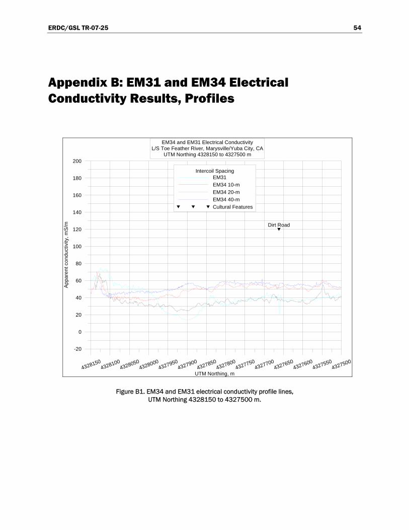
ERDC/GSL TR-07-25 54
Appendix B: EM31 and EM34 Electrical Conductivity Results, Profiles
43281504328100
43280504328000
43279504327900
43278504327800
43277504327700
43276504327600
43275504327500
UTM Northing, m
-20
0
20
40
60
80
100
120
140
160
180
200
Appa
rent
con
duct
ivity
, mS/
m
Intercoil SpacingEM31EM34 10-mEM34 20-mEM34 40-mCultural Features
Dirt Road
EM34 and EM31 Electrical ConductivityL/S Toe Feather River, Marysville/Yuba City, CA
UTM Northing 4328150 to 4327500 m
Figure B1. EM34 and EM31 electrical conductivity profile lines, UTM Northing 4328150 to 4327500 m.
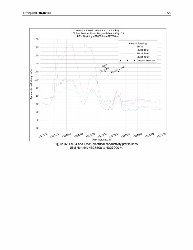
ERDC/GSL TR-07-25 55
43275004327450
43274004327350
43273004327250
43272004327150
43271004327050
4327000
UTM Northing, m
-20
0
20
40
60
80
100
120
140
160
180
200
Appa
rent
con
duct
ivity
, mS/
m
Intercoil SpacingEM31EM34 10-mEM34 20-mEM34 40-mCultural Features
Dirt RoadTrash
Grassy Road
EM34 and EM31 Electrical ConductivityL/S Toe Feather River, Marysville/Yuba City, CA
UTM Northing 4328500 to 4327000 m
Figure B2. EM34 and EM31 electrical conductivity profile lines,
UTM Northing 4327500 to 4327000 m.

ERDC/GSL TR-07-25 56
43270004326950
43269004326850
43268004326750
43267004326650
43266004326550
4326500
UTM Northing, m
-20
0
20
40
60
80
100
120
140
160
180
200
Appa
rent
con
duct
ivity
, mS/
m
Intercoil SpacingEM31EM34 10-mEM34 20-mEM34 40-mCultural Features
Ramp Trash
EM34 and EM31 Electrical ConductivityL/S Toe Feather River, Marysville/Yuba City, CA
UTM Northing 4327000 to 4326500 m
Figure B3. EM34 and EM31 electrical conductivity profile lines,
UTM Northing 4327000 to 4326500 m.

ERDC/GSL TR-07-25 57
43265004326450
43264004326350
43263004326250
43262004326150
43261004326050
4326000
UTM Northing, m
-20
0
20
40
60
80
100
120
140
160
180
200
Appa
rent
con
duct
ivity
, mS/
m
Intercoil SpacingEM31EM34 10-mEM34 20-mEM34 40-mCultural Features
Trash Ramp Trash Trash
EM34 and EM31 Electrical ConductivityL/S Toe Feather River, Marysville/Yuba City, CA
UTM Northing 4326500 to 4326000 m
Figure B4. EM34 and EM31 electrical conductivity profile lines,
UTM Northing 4326500 to 4326000 m.

ERDC/GSL TR-07-25 58
43260004325950
43259004325850
43258004325750
43257004325650
43256004325550
4325500
UTM Northing, m
-20
0
20
40
60
80
100
120
140
160
180
200
Appa
rent
con
duct
ivity
, mS
/m
Intercoil SpacingEM31EM34 10-mEM34 20-mEM34 40-mCultural Features
Tras
h
Deb
ris
Deb
risH
igh-
tens
ion
Pow
er L
ines
Ber
m
Gra
vel R
oad
EM34 and EM31 Electrical ConductivityL/S Toe Feather River, Marysville/Yuba City, CA
UTM Northing 4326000 to 4325500 m
Figure B5. EM34 and EM31 electrical conductivity profile lines,
UTM Northing 4326000 to 4325500 m.

ERDC/GSL TR-07-25 59
43255004325450
43254004325350
43253004325250
43252004325150
43251004325050
4325000
UTM Northing, m
-20
0
20
40
60
80
100
120
140
160
180
200
Appa
rent
con
duct
ivity
, mS/
m
Intercoil SpacingEM31EM34 10-mEM34 20-mEM34 40-mCultural Features
Steel Standpipe
EM34 and EM31 Electrical ConductivityL/S Toe Feather River, Marysville/Yuba City, CA
UTM Northing 4325500 to 4325000 m
Figure B6. EM34 and EM31 electrical conductivity profile lines,
UTM Northing 4325500 to 4325000 m.

ERDC/GSL TR-07-25 60
43250004324950
43249004324850
43248004324750
43247004324650
43246004324550
4324500
UTM Northing, m
-20
0
20
40
60
80
100
120
140
160
180
200
Appa
rent
con
duct
ivity
, mS/
m
Intercoil SpacingEM31EM34 10-mEM34 20-mEM34 40-mCultural Features
Ramp Dirt Road
EM34 and EM31 Electrical ConductivityL/S Toe Feather River, Marysville/Yuba City, CA
UTM Northing 4325000 to 4324500 m
Figure B7. EM34 and EM31 electrical conductivity profile lines,
UTM Northing 4325000 to 4324500 m.

ERDC/GSL TR-07-25 61
43245004324450
43244004324350
43243004324250
43242004324150
43241004324050
4324000
UTM Northing, m
-20
0
20
40
60
80
100
120
140
160
180
200
Appa
rent
con
duct
ivity
, mS/
m
Intercoil SpacingEM31EM34 10-mEM34 20-mEM34 40-mCultural Features
Ramp
Trash
Trash
Trash
N-end of Trash
S-end of Trash
EM34 and EM31 Electrical ConductivityL/S Toe Feather River, Marysville/Yuba City, CA
UTM Northing 4324500 to 4324000 m
Figure B8. EM34 and EM31 electrical conductivity profile lines,
UTM Northing 4324500 to 4324000 m.

ERDC/GSL TR-07-25 62
43240004323950
43239004323850
43238004323750
43237004323650
43236004323550
4323500
UTM Northing, m
-20
0
20
40
60
80
100
120
140
160
180
200
Appa
rent
con
duct
ivity
, mS/
m
Intercoil SpacingEM31EM34 10-mEM34 20-mEM34 40-mCultural Features
Well Ramp
EM34 and EM31 Electrical ConductivityL/S Toe Feather River, Marysville/Yuba City, CA
UTM Northing 4324000 to 4323500 m
Figure B9. EM34 and EM31 electrical conductivity profile lines,
UTM Northing 4324000 to 4323500 m.
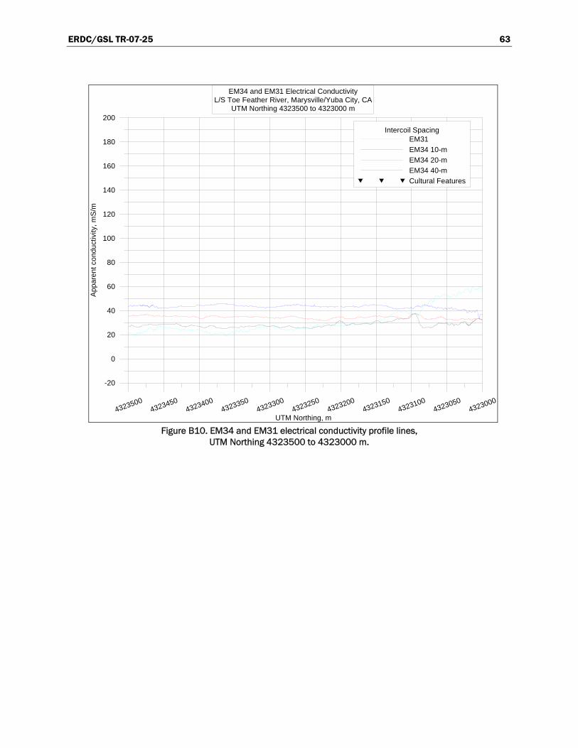
ERDC/GSL TR-07-25 63
43235004323450
43234004323350
43233004323250
43232004323150
43231004323050
4323000
UTM Northing, m
-20
0
20
40
60
80
100
120
140
160
180
200
Appa
rent
con
duct
ivity
, mS/
m
Intercoil SpacingEM31EM34 10-mEM34 20-mEM34 40-mCultural Features
EM34 and EM31 Electrical ConductivityL/S Toe Feather River, Marysville/Yuba City, CA
UTM Northing 4323500 to 4323000 m
Figure B10. EM34 and EM31 electrical conductivity profile lines,
UTM Northing 4323500 to 4323000 m.

ERDC/GSL TR-07-25 64
43230004322950
43229004322850
43228004322750
43227004322650
43226004322550
4322500
UTM Northing, m
-20
0
20
40
60
80
100
120
140
160
180
200
Appa
rent
con
duct
ivity
, mS/
m
Intercoil SpacingEM31EM34 10-mEM34 20-mEM34 40-mCultural Features
Ramp Trash
EM34 and EM31 Electrical ConductivityL/S Toe Feather River, Marysville/Yuba City, CA
UTM Northing 4323000 to 4322500 m
Figure B11. EM34 and EM31 electrical conductivity profile lines,
UTM Northing 4323000 to 4322500 m.
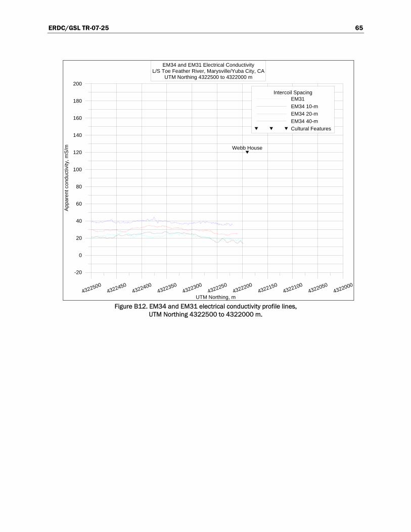
ERDC/GSL TR-07-25 65
43225004322450
43224004322350
43223004322250
43222004322150
43221004322050
4322000
UTM Northing, m
-20
0
20
40
60
80
100
120
140
160
180
200
Appa
rent
con
duct
ivity
, mS/
m
Intercoil SpacingEM31EM34 10-mEM34 20-mEM34 40-mCultural Features
Webb House
EM34 and EM31 Electrical ConductivityL/S Toe Feather River, Marysville/Yuba City, CA
UTM Northing 4322500 to 4322000 m
Figure B12. EM34 and EM31 electrical conductivity profile lines,
UTM Northing 4322500 to 4322000 m.

ERDC/GSL TR-07-25 66
43220004321950
43219004321850
43218004321750
43217004321650
43216004321550
4321500
UTM Northing, m
-20
0
20
40
60
80
100
120
140
160
180
200
Appa
rent
con
duct
ivity
, mS/
m
Intercoil SpacingEM31EM34 10-mEM34 20-mEM34 40-mCultural Features
Pole Pump
EM34 and EM31 Electrical ConductivityL/S Toe Feather River, Marysville/Yuba City, CA
UTM Northing 4322000 to 4321500 m
Figure B13. EM34 and EM31 electrical conductivity profile lines,
UTM Northing 4322000 to 4321500 m.
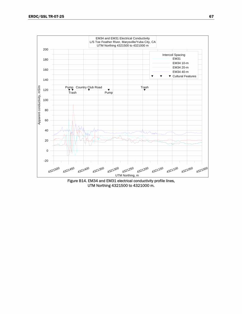
ERDC/GSL TR-07-25 67
43215004321450
43214004321350
43213004321250
43212004321150
43211004321050
4321000
UTM Northing, m
-20
0
20
40
60
80
100
120
140
160
180
200
Appa
rent
con
duct
ivity
, mS/
m
Intercoil SpacingEM31EM34 10-mEM34 20-mEM34 40-mCultural Features
Pump
Trash
Country Club Road
Pump
Trash
EM34 and EM31 Electrical ConductivityL/S Toe Feather River, Marysville/Yuba City, CA
UTM Northing 4321500 to 4321000 m
Figure B14. EM34 and EM31 electrical conductivity profile lines,
UTM Northing 4321500 to 4321000 m.

ERDC/GSL TR-07-25 68
43210004320950
43209004320850
43208004320750
43207004320650
43206004320550
4320500
UTM Northing, m
-20
0
20
40
60
80
100
120
140
160
180
200
Appa
rent
con
duct
ivity
, mS/
m
Intercoil SpacingEM31EM34 10-mEM34 20-mEM34 40-mCultural Features
Porta-John
EM34 and EM31 Electrical ConductivityL/S Toe Feather River, Marysville/Yuba City, CA
UTM Northing 4321000 to 4320500 m
Figure B15. EM34 and EM31 electrical conductivity profile lines,
UTM Northing 4321000 to 4320500 m.

ERDC/GSL TR-07-25 69
43205004320450
43204004320350
43203004320250
43202004320150
43201004320050
4320000
UTM Northing, m
-20
0
20
40
60
80
100
120
140
160
180
200
Appa
rent
con
duct
ivity
, mS/
m
Intercoil SpacingEM31EM34 10-mEM34 20-mEM34 40-mCultural Features
Ramp
EM34 and EM31 Electrical ConductivityL/S Toe Feather River, Marysville/Yuba City, CA
UTM Northing 4320500 to 4320000 m
Figure B16. EM34 and EM31 electrical conductivity profile lines,
UTM Northing 4320500 to 4320000 m.
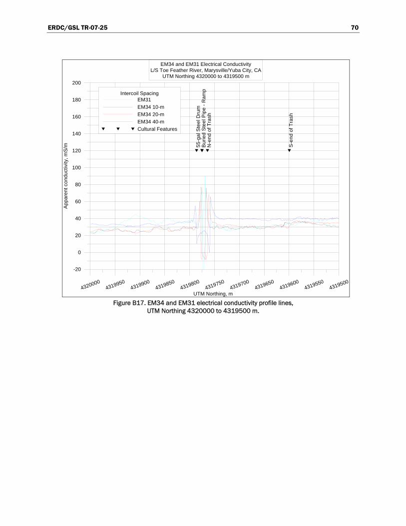
ERDC/GSL TR-07-25 70
43200004319950
43199004319850
43198004319750
43197004319650
43196004319550
4319500
UTM Northing, m
-20
0
20
40
60
80
100
120
140
160
180
200
Appa
rent
con
duct
ivity
, mS/
m
Intercoil SpacingEM31EM34 10-mEM34 20-mEM34 40-mCultural Features
55-g
al S
teel
Dru
mB
urie
d St
eel P
ipe
- Ram
pN
-end
of T
rash
S-e
nd o
f Tra
sh
EM34 and EM31 Electrical ConductivityL/S Toe Feather River, Marysville/Yuba City, CA
UTM Northing 4320000 to 4319500 m
Figure B17. EM34 and EM31 electrical conductivity profile lines,
UTM Northing 4320000 to 4319500 m.
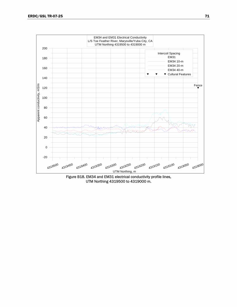
ERDC/GSL TR-07-25 71
43195004319450
43194004319350
43193004319250
43192004319150
43191004319050
4319000
UTM Northing, m
-20
0
20
40
60
80
100
120
140
160
180
200
Appa
rent
con
duct
ivity
, mS/
m
Intercoil SpacingEM31EM34 10-mEM34 20-mEM34 40-mCultural Features
Fence
EM34 and EM31 Electrical ConductivityL/S Toe Feather River, Marysville/Yuba City, CA
UTM Northing 4319500 to 4319000 m
Figure B18. EM34 and EM31 electrical conductivity profile lines,
UTM Northing 4319500 to 4319000 m.
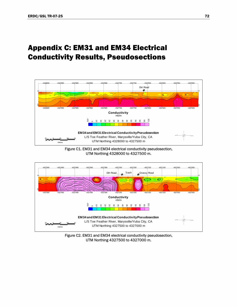
ERDC/GSL TR-07-25 72
Appendix C: EM31 and EM34 Electrical Conductivity Results, Pseudosections
Figure C1. EM31 and EM34 electrical conductivity pseudosection, UTM Northing 4328000 to 4327500 m.
Figure C2. EM31 and EM34 electrical conductivity pseudosection, UTM Northing 4327500 to 4327000 m.
25 0 25 50 75
metres
EM34 and EM31 Electrical Conductivity PseudosectionL/S Toe Feather River, Marysville/Yuba City, CA
UTM Northing 4328000 to 4327500 m
-101
3215 10 15 20 25 30 35 40 45 50 55 60 65
ConductivitymS/m
-50
0-50
0
-4328000 -4327950 -4327900 -4327850 -4327800 -4327750 -4327700 -4327650 -4327600 -4327550 -4327500
-4328000 -4327950 -4327900 -4327850 -4327800 -4327750 -4327700 -4327650 -4327600 -4327550 -4327500
Dirt Road
25
0 5
0 5
25 0 25 50 75
metres
EM34 and EM31 Electrical Conductivity PseudosectionL/S Toe Feather River, Marysville/Yuba City, CA
UTM Northing 4327500 to 4327000 m
-101
3215 10 15 20 25 30 35 40 45 50 55 60 65
ConductivitymS/m
-50
0-50
0
-4327500 -4327450 -4327400 -4327350 -4327300 -4327250 -4327200 -4327150 -4327100 -4327050 -4327000
-4327500 -4327450 -4327400 -4327350 -4327300 -4327250 -4327200 -4327150 -4327100 -4327050 -4327000
Grassy RoadDirt Road Trash
5 2
05
05
50 0 5 1
0 0 20 5 2

ERDC/GSL TR-07-25 73
Figure C3. EM31 and EM34 electrical conductivity pseudosection, UTM Northing 4327000 to 4326500 m.
Figure C4. EM31 and EM34 electrical conductivity pseudosection, UTM Northing 4326500 to 4326000 m.
Figure C5. EM31 and EM34 electrical conductivity pseudosection, UTM Northing 4326000 to 4325500 m.
25 0 25 50 75
metres
EM34 and EM31 Electrical Conductivity PseudosectionL/S Toe Feather River, Marysville/Yuba City, CA
UTM Northing 4327000 to 4326500 m
-101
3215 10 15 20 25 30 35 40 45 50 55 60 65
ConductivitymS/m
-50
0-50
0
-4327000 -4326950 -4326900 -4326850 -4326800 -4326750 -4326700 -4326650 -4326600 -4326550 -4326500
-4327000 -4326950 -4326900 -4326850 -4326800 -4326750 -4326700 -4326650 -4326600 -4326550 -4326500
TrashRamp Trash
2525
25 0 25 50 75
metres
EM34 and EM31 Electrical Conductivity PseudosectionL/S Toe Feather River, Marysville/Yuba City, CA
UTM Northing 4326500 to 4326000 m
-101
3215 10 15 20 25 30 35 40 45 50 55 60 65
ConductivitymS/m
-50
0-50
0
-4326500 -4326450 -4326400 -4326350 -4326300 -4326250 -4326200 -4326150 -4326100 -4326050 -4326000
-4326500 -4326450 -4326400 -4326350 -4326300 -4326250 -4326200 -4326150 -4326100 -4326050 -4326000
TrashRampTrash
2525
25 0 25 50 75
metres
EM34 and EM31 Electrical Conductivity PseudosectionL/S Toe Feather River, Marysville/Yuba City, CA
UTM Northing 4326000 to 4325500 m
-101
3215 10 15 20 25 30 35 40 45 50 55 60 65
ConductivitymS/m
-50
0-50
0
-4326000 -4325950 -4325900 -4325850 -4325800 -4325750 -4325700 -4325650 -4325600 -4325550 -4325500
-4326000 -4325950 -4325900 -4325850 -4325800 -4325750 -4325700 -4325650 -4325600 -4325550 -4325500
Gravel Road (Ella Road?)
High-Tension Pow er Line CrossingTrash Piles
Trash
2 5
2525

ERDC/GSL TR-07-25 74
25 0 25 50 75
metres
EM34 and EM31 Electrical Conductivity PseudosectionL/S Toe Feather River, Marysville/Yuba City, CA
UTM Northing 4325500 to 4325000 m
-101
3215 10 15 20 25 30 35 40 45 50 55 60 65
ConductivitymS/m
-50
0-50
0
-4325500 -4325450 -4325400 -4325350 -4325300 -4325250 -4325200 -4325150 -4325100 -4325050 -4325000
-4325500 -4325450 -4325400 -4325350 -4325300 -4325250 -4325200 -4325150 -4325100 -4325050 -4325000
1.2 m Diameter Corrugated Steel Standpipe
2525
2525
Figure C6. EM31 and EM34 electrical conductivity pseudosection,
UTM Northing 4325500 to 4325000 m.
Figure C7. EM31 and EM34 electrical conductivity pseudosection, UTM Northing 4325000 to 4324500 m.
Figure C8. EM31 and EM34 electrical conductivity pseudosection, UTM Northing 4324500 to 4324000 m.
25 0 25 50 75
metres
EM34 and EM31 Electrical Conductivity PseudosectionL/S Toe Feather River, Marysville/Yuba City, CA
UTM Northing 4325000 to 4324500 m
-101
3215 10 15 20 25 30 35 40 45 50 55 60 65
ConductivitymS/m
-50
0-50
0
-4325000 -4324950 -4324900 -4324850 -4324800 -4324750 -4324700 -4324650 -4324600 -4324550 -4324500
-4325000 -4324950 -4324900 -4324850 -4324800 -4324750 -4324700 -4324650 -4324600 -4324550 -4324500
Dirt RoadRamp
25 25 25
25 0 25 50 75
metres
EM34 and EM31 Electrical Conductivity PseudosectionL/S Toe Feather River, Marysville/Yuba City, CA
UTM Northing 4324500 to 4324000 m
-101
3215 10 15 20 25 30 35 40 45 50 55 60 65
ConductivitymS/m
-50
0-50
0
-4324500 -4324450 -4324400 -4324350 -4324300 -4324250 -4324200 -4324150 -4324100 -4324050 -4324000
-4324500 -4324450 -4324400 -4324350 -4324300 -4324250 -4324200 -4324150 -4324100 -4324050 -4324000
Trash PileTrash PilesRamp
2525
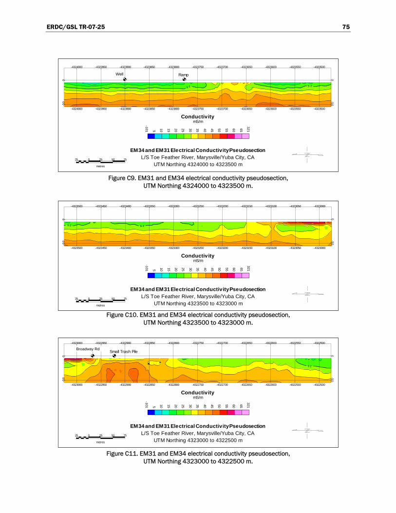
ERDC/GSL TR-07-25 75
Figure C9. EM31 and EM34 electrical conductivity pseudosection, UTM Northing 4324000 to 4323500 m.
Figure C10. EM31 and EM34 electrical conductivity pseudosection, UTM Northing 4323500 to 4323000 m.
Figure C11. EM31 and EM34 electrical conductivity pseudosection, UTM Northing 4323000 to 4322500 m.
25 0 25 50 75
metres
EM34 and EM31 Electrical Conductivity PseudosectionL/S Toe Feather River, Marysville/Yuba City, CA
UTM Northing 4324000 to 4323500 m
-101
3215 10 15 20 25 30 35 40 45 50 55 60 65
ConductivitymS/m
-50
0-50
0
-4324000 -4323950 -4323900 -4323850 -4323800 -4323750 -4323700 -4323650 -4323600 -4323550 -4323500
-4324000 -4323950 -4323900 -4323850 -4323800 -4323750 -4323700 -4323650 -4323600 -4323550 -4323500
RampWell
25 25
25 0 25 50 75
metres
EM34 and EM31 Electrical Conductivity PseudosectionL/S Toe Feather River, Marysville/Yuba City, CA
UTM Northing 4323500 to 4323000 m
-101
3215 10 15 20 25 30 35 40 45 50 55 60 65
ConductivitymS/m
-50
0-50
0
-4323500 -4323450 -4323400 -4323350 -4323300 -4323250 -4323200 -4323150 -4323100 -4323050 -4323000
-4323500 -4323450 -4323400 -4323350 -4323300 -4323250 -4323200 -4323150 -4323100 -4323050 -4323000
2525
25 0 25 50 75
metres
EM34 and EM31 Electrical Conductivity PseudosectionL/S Toe Feather River, Marysville/Yuba City, CA
UTM Northing 4323000 to 4322500 m
-101
3215 10 15 20 25 30 35 40 45 50 55 60 65
ConductivitymS/m
-50
0-50
0
-4323000 -4322950 -4322900 -4322850 -4322800 -4322750 -4322700 -4322650 -4322600 -4322550 -4322500
-4323000 -4322950 -4322900 -4322850 -4322800 -4322750 -4322700 -4322650 -4322600 -4322550 -4322500
Small Trash PileBroadw ay Rd.
25
Broadway Rd

ERDC/GSL TR-07-25 76
Figure C12. EM31 and EM34 electrical conductivity pseudosection, UTM Northing 4322500 to 4322000 m.
Figure C13. EM31 and EM34 electrical conductivity pseudosection, UTM Northing 4322000 to 4321500 m.
Figure C14. EM31 and EM34 electrical conductivity pseudosection, UTM Northing 4321500 to 4321000 m.
25 0 25 50 75
metres
EM34 and EM31 Electrical Conductivity PseudosectionL/S Toe Feather River, Marysville/Yuba City, CA
UTM Northing 4322500 to 4322000 m
-101
3215 10 15 20 25 30 35 40 45 50 55 60 65
ConductivitymS/m
-50
0-50
0
-4322500 -4322450 -4322400 -4322350 -4322300 -4322250 -4322200 -4322150 -4322100 -4322050 -4322000
-4322500 -4322450 -4322400 -4322350 -4322300 -4322250 -4322200 -4322150 -4322100 -4322050 -4322000
Inaccessible - No DataAnderson Ave.
25
25
25 0 25 50 75
metres
EM34 and EM31 Electrical Conductivity PseudosectionL/S Toe Feather River, Marysville/Yuba City, CA
UTM Northing 4322000 to 4321500 m
-101
3215 10 15 20 25 30 35 40 45 50 55 60 65
ConductivitymS/m
-50
0-50
0
-4322000 -4321950 -4321900 -4321850 -4321800 -4321750 -4321700 -4321650 -4321600 -4321550 -4321500
-4322000 -4321950 -4321900 -4321850 -4321800 -4321750 -4321700 -4321650 -4321600 -4321550 -4321500
PumpPow er Pole
2525
25 0 25 50 75
metres
EM34 and EM31 Electrical Conductivity PseudosectionL/S Toe Feather River, Marysville/Yuba City, CA
UTM Northing 4321500 to 4321000 m
-101
3215 10 15 20 25 30 35 40 45 50 55 60 65
ConductivitymS/m
-50
0-50
0
-4321500 -4321450 -4321400 -4321350 -4321300 -4321250 -4321200 -4321150 -4321100 -4321050 -4321000
-4321500 -4321450 -4321400 -4321350 -4321300 -4321250 -4321200 -4321150 -4321100 -4321050 -4321000
Trash PileWater PumpCountry Club Lane
Water Pump
25 2525

ERDC/GSL TR-07-25 77
Figure C15. EM31 and EM34 electrical conductivity pseudosection, UTM Northing 4321000 to 4320500 m.
Figure C16. EM31 and EM34 electrical conductivity pseudosection, UTM Northing 4320500 to 4320000 m.
Figure C17. EM31 and EM34 electrical conductivity pseudosection, UTM Northing 4320000 to 4319500 m.
25 0 25 50 75
metres
EM34 and EM31 Electrical Conductivity PseudosectionL/S Toe Feather River, Marysville/Yuba City, CA
UTM Northing 4321000 to 4320500 m
-101
3215 10 15 20 25 30 35 40 45 50 55 60 65
ConductivitymS/m
-50
0-50
0
-4321000 -4320950 -4320900 -4320850 -4320800 -4320750 -4320700 -4320650 -4320600 -4320550 -4320500
-4321000 -4320950 -4320900 -4320850 -4320800 -4320750 -4320700 -4320650 -4320600 -4320550 -4320500
Inaccessible Area - No Data
25 5 2
25 0 25 50 75
metres
EM34 and EM31 Electrical Conductivity PseudosectionL/S Toe Feather River, Marysville/Yuba City, CA
UTM Northing 4320500 to 4320000 m
-101
3215 10 15 20 25 30 35 40 45 50 55 60 65
ConductivitymS/m
-50
0-50
0
-4320500 -4320450 -4320400 -4320350 -4320300 -4320250 -4320200 -4320150 -4320100 -4320050 -4320000
-4320500 -4320450 -4320400 -4320350 -4320300 -4320250 -4320200 -4320150 -4320100 -4320050 -4320000
Ramp
5 2 5 2
25 0 25 50 75
metres
EM34 and EM31 Electrical Conductivity PseudosectionL/S Toe Feather River, Marysville/Yuba City, CA
UTM Northing 4320000 to 4319500 m
-101
3215 10 15 20 25 30 35 40 45 50 55 60 65
ConductivitymS/m
-50
0-50
0
-4320000 -4319950 -4319900 -4319850 -4319800 -4319750 -4319700 -4319650 -4319600 -4319550 -4319500
-4320000 -4319950 -4319900 -4319850 -4319800 -4319750 -4319700 -4319650 -4319600 -4319550 -4319500
Steel Pipeline55-Gal. Steel Drum
5 2
52
5 2

ERDC/GSL TR-07-25 78
Figure C18. EM31 and EM34 electrical conductivity pseudosection, UTM Northing 4319500 to 4319000 m.
25 0 25 50 75
metres
EM34 and EM31 Electrical Conductivity PseudosectionL/S Toe Feather River, Marysville/Yuba City, CA
UTM Northing 4319500 to 4319000 m
-101
3215 10 15 20 25 30 35 40 45 50 55 60 65
ConductivitymS/m
-50
0-50
0
-4319500 -4319450 -4319400 -4319350 -4319300 -4319250 -4319200 -4319150 -4319100 -4319050 -4319000
-4319500 -4319450 -4319400 -4319350 -4319300 -4319250 -4319200 -4319150 -4319100 -4319050 -4319000
N End of Fence
05
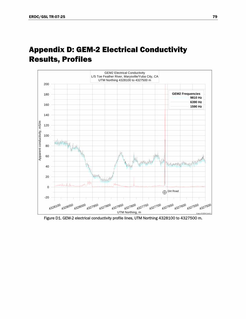
ERDC/GSL TR-07-25 79
Appendix D: GEM-2 Electrical Conductivity Results, Profiles
43281004328050
43280004327950
43279004327850
43278004327750
43277004327650
43276004327550
4327500
UTM Northing, m
-20
0
20
40
60
80
100
120
140
160
180
200
App
aren
t con
duct
ivity
, mS
/m
GEM2 Frequencies9810 Hz6390 Hz1590 Hz
GEM2 Electrical ConductivityL/S Toe Feather River, Marysville/Yuba City, CA
UTM Northing 4328100 to 4327500 m
Copy of GEM Cond 1
Dirt Road
Figure D1. GEM-2 electrical conductivity profile lines, UTM Northing 4328100 to 4327500 m.

ERDC/GSL TR-07-25 80
43275004327450
43274004327350
43273004327250
43272004327150
43271004327050
4327000
UTM Northing, m
-20
0
20
40
60
80
100
120
140
160
180
200
App
aren
t con
duct
ivity
, mS
/m
GEM2 Frequencies9810 Hz6390 Hz1590 Hz
GEM2 Electrical ConductivityL/S Toe Feather River, Marysville/Yuba City, CA
UTM Northing 4327500 to 4327000 m
Copy of GEM Cond 2
Dirt Road
Trash Grassy Road
Figure D2. GEM-2 electrical conductivity profile lines, UTM Northing 4327500 to 4327000 m.

ERDC/GSL TR-07-25 81
43270004326950
43269004326850
43268004326750
43267004326650
43266004326550
4326500
UTM Northing, m
-20
0
20
40
60
80
100
120
140
160
180
200
App
aren
t con
duct
ivity
, mS
/m
GEM2 Frequencies9810 Hz6390 Hz1590 Hz
GEM2 Electrical ConductivityL/S Toe Feather River, Marysville/Yuba City, CA
UTM Northing 4327000 to 4326500 m
Copy of GEM Cond 3
Ramp Trash
Figure D3. GEM-2 electrical conductivity profile lines, UTM Northing 4327000 to 4326500 m.
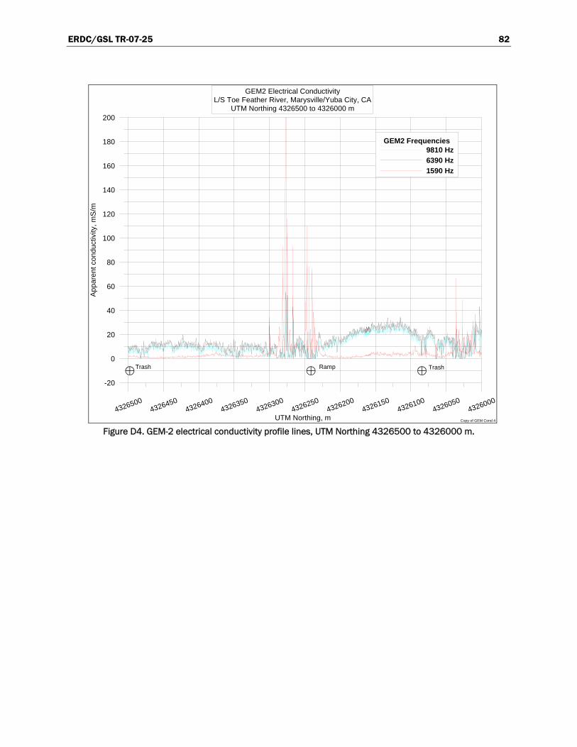
ERDC/GSL TR-07-25 82
43265004326450
43264004326350
43263004326250
43262004326150
43261004326050
4326000
UTM Northing, m
-20
0
20
40
60
80
100
120
140
160
180
200
App
aren
t con
duct
ivity
, mS
/m
GEM2 Frequencies9810 Hz6390 Hz1590 Hz
GEM2 Electrical ConductivityL/S Toe Feather River, Marysville/Yuba City, CA
UTM Northing 4326500 to 4326000 m
Copy of GEM Cond 4
Trash TrashRamp
Figure D4. GEM-2 electrical conductivity profile lines, UTM Northing 4326500 to 4326000 m.
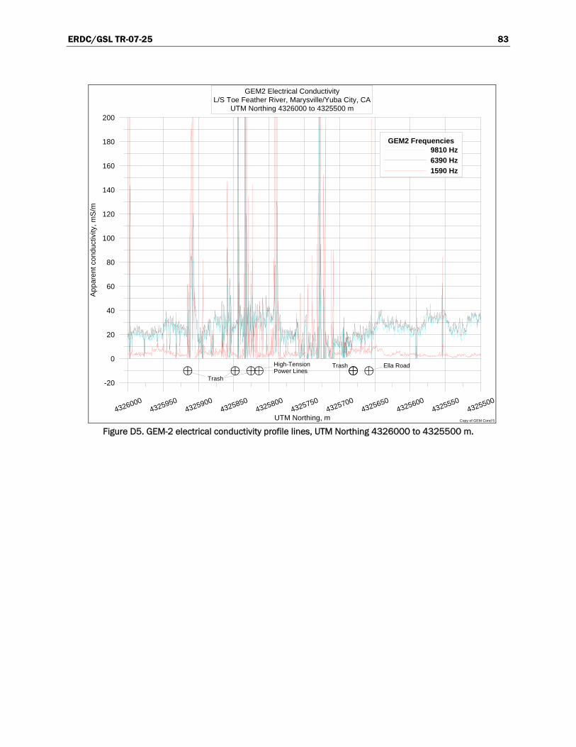
ERDC/GSL TR-07-25 83
43260004325950
43259004325850
43258004325750
43257004325650
43256004325550
4325500
UTM Northing, m
-20
0
20
40
60
80
100
120
140
160
180
200
App
aren
t con
duct
ivity
, mS
/m
GEM2 Frequencies9810 Hz6390 Hz1590 Hz
GEM2 Electrical ConductivityL/S Toe Feather River, Marysville/Yuba City, CA
UTM Northing 4326000 to 4325500 m
Copy of GEM Cond 5
Trash
High-TensionPower Lines
Trash Ella Road
Figure D5. GEM-2 electrical conductivity profile lines, UTM Northing 4326000 to 4325500 m.

ERDC/GSL TR-07-25 84
43255004325450
43254004325350
43253004325250
43252004325150
43251004325050
4325000
UTM Northing, m
-20
0
20
40
60
80
100
120
140
160
180
200
App
aren
t con
duct
ivity
, mS
/m
GEM2 Frequencies9810 Hz6390 Hz1590 Hz
GEM2 Electrical ConductivityL/S Toe Feather River, Marysville/Yuba City, CA
UTM Northing 4325500 to 4325000 m
Copy of GEM Cond 6
1.2-m Diameter CorrugatedSteel Standpipe
Figure D6. GEM-2 electrical conductivity profile lines, UTM Northing 4325500 to 4325000 m.
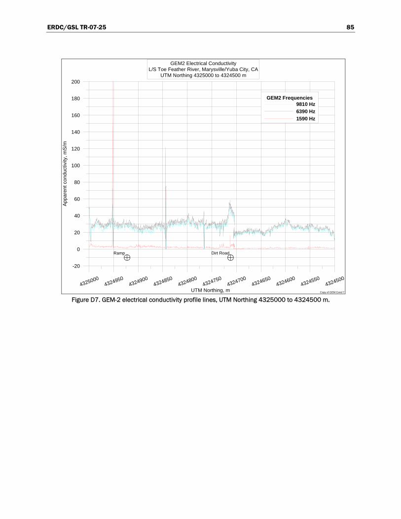
ERDC/GSL TR-07-25 85
43250004324950
43249004324850
43248004324750
43247004324650
43246004324550
4324500
UTM Northing, m
-20
0
20
40
60
80
100
120
140
160
180
200
App
aren
t con
duct
ivity
, mS
/m
GEM2 Frequencies9810 Hz6390 Hz1590 Hz
GEM2 Electrical ConductivityL/S Toe Feather River, Marysville/Yuba City, CA
UTM Northing 4325000 to 4324500 m
Copy of GEM Cond 7
Ramp Dirt Road
Figure D7. GEM-2 electrical conductivity profile lines, UTM Northing 4325000 to 4324500 m.

ERDC/GSL TR-07-25 86
43245004324450
43244004324350
43243004324250
43242004324150
43241004324050
4324000
UTM Northing, m
-20
0
20
40
60
80
100
120
140
160
180
200
App
aren
t con
duct
ivity
, mS
/m
GEM2 Frequencies9810 Hz6390 Hz1590 Hz
GEM2 Electrical ConductivityL/S Toe Feather River, Marysville/Yuba City, CA
UTM Northing 4324500 to 4324000 m
Copy of GEM Cond 8
Trash PileTrash PilesRamp
Figure D8. GEM-2 electrical conductivity profile lines, UTM Northing 4324500 to 4324000 m.

ERDC/GSL TR-07-25 87
43240004323950
43239004323850
43238004323750
43237004323650
43236004323550
4323500
UTM Northing, m
-20
0
20
40
60
80
100
120
140
160
180
200
App
aren
t con
duct
ivity
, mS
/m
GEM2 Frequencies9810 Hz6390 Hz1590 Hz
GEM2 Electrical ConductivityL/S Toe Feather River, Marysville/Yuba City, CA
UTM Northing 4324000 to 4323500 m
Copy of GEM Cond 9
RampWell
Figure D9. GEM-2 electrical conductivity profile lines, UTM Northing 4324000 to 4323500 m.

ERDC/GSL TR-07-25 88
43235004323450
43234004323350
43233004323250
43232004323150
43231004323050
4323000
UTM Northing, m
-20
0
20
40
60
80
100
120
140
160
180
200
App
aren
t con
duct
ivity
, mS
/m
GEM2 Frequencies9810 Hz6390 Hz1590 Hz
GEM2 Electrical ConductivityL/S Toe Feather River, Marysville/Yuba City, CA
UTM Northing 4323500 to 4323000 m
Copy of GEM Cond 10 Figure D10. GEM-2 electrical conductivity profile lines,
UTM Northing 4323500 to 4323000 m.
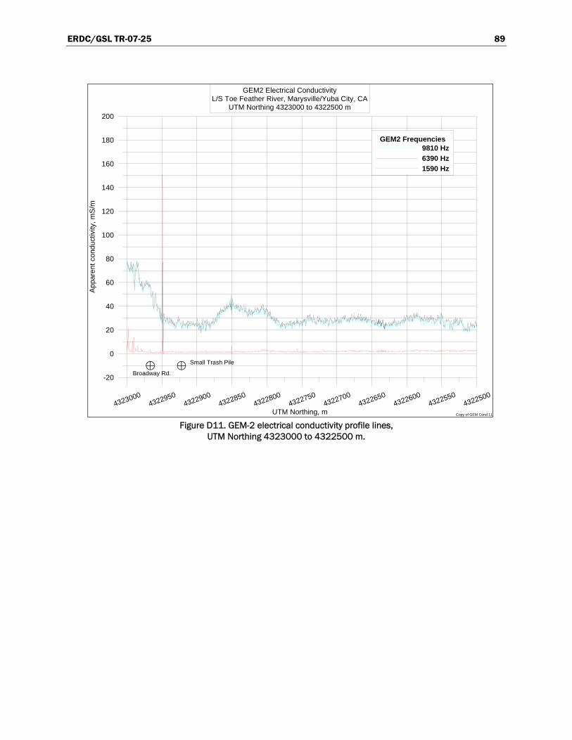
ERDC/GSL TR-07-25 89
43230004322950
43229004322850
43228004322750
43227004322650
43226004322550
4322500
UTM Northing, m
-20
0
20
40
60
80
100
120
140
160
180
200
App
aren
t con
duct
ivity
, mS
/m
GEM2 Frequencies9810 Hz6390 Hz1590 Hz
GEM2 Electrical ConductivityL/S Toe Feather River, Marysville/Yuba City, CA
UTM Northing 4323000 to 4322500 m
Copy of GEM Cond 11
Broadway Rd.
Small Trash Pile
Figure D11. GEM-2 electrical conductivity profile lines,
UTM Northing 4323000 to 4322500 m.

ERDC/GSL TR-07-25 90
43225004322450
43224004322350
43223004322250
43222004322150
43221004322050
4322000
UTM Northing, m
-20
0
20
40
60
80
100
120
140
160
180
200
App
aren
t con
duct
ivity
, mS
/m
GEM2 Frequencies9810 Hz6390 Hz1590 Hz
GEM2 Electrical ConductivityL/S Toe Feather River, Marysville/Yuba City, CA
UTM Northing 4322500 to 4322000 m
Copy of GEM Cond 12
Anderson Ave.
InaccessibleNo Data
Figure D12. GEM-2 electrical conductivity profile lines,
UTM Northing 4322500 to 4322000 m.

ERDC/GSL TR-07-25 91
43220004321950
43219004321850
43218004321750
43217004321650
43216004321550
4321500
UTM Northing, m
-20
0
20
40
60
80
100
120
140
160
180
200
App
aren
t con
duct
ivity
, mS
/m
GEM2 Frequencies9810 Hz6390 Hz1590 Hz
GEM2 Electrical ConductivityL/S Toe Feather River, Marysville/Yuba City, CA
UTM Northing 4322000 to 4321500 m
Copy of GEM Cond 13
Power Pole Pump
Figure D13. GEM-2 electrical conductivity profile lines,
UTM Northing 4322000 to 4321500 m.

ERDC/GSL TR-07-25 92
43215004321450
43214004321350
43213004321250
43212004321150
43211004321050
4321000
UTM Northing, m
-20
0
20
40
60
80
100
120
140
160
180
200
App
aren
t con
duct
ivity
, mS
/m
GEM2 Frequencies9810 Hz6390 Hz1590 Hz
GEM2 Electrical ConductivityL/S Toe Feather River, Marysville/Yuba City, CA
UTM Northing 4321500 to 4321000 m
Copy of GEM Cond 14
Water Pump Trash
Country Club Lane
Water Pump
Trash Pile
Figure D14. GEM-2 electrical conductivity profile lines,
UTM Northing 4321500 to 4321000 m.
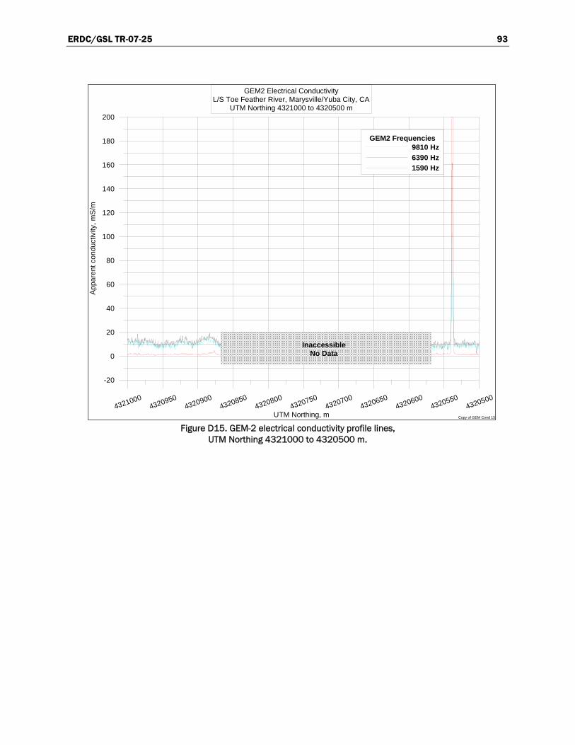
ERDC/GSL TR-07-25 93
43210004320950
43209004320850
43208004320750
43207004320650
43206004320550
4320500
UTM Northing, m
-20
0
20
40
60
80
100
120
140
160
180
200
App
aren
t con
duct
ivity
, mS
/m
GEM2 Frequencies9810 Hz6390 Hz1590 Hz
GEM2 Electrical ConductivityL/S Toe Feather River, Marysville/Yuba City, CA
UTM Northing 4321000 to 4320500 m
Copy of GEM Cond 15
InaccessibleNo Data
Figure D15. GEM-2 electrical conductivity profile lines,
UTM Northing 4321000 to 4320500 m.

ERDC/GSL TR-07-25 94
43205004320450
43204004320350
43203004320250
43202004320150
43201004320050
4320000
UTM Northing, m
-20
0
20
40
60
80
100
120
140
160
180
200
App
aren
t con
duct
ivity
, mS
/m
GEM2 Frequencies9810 Hz6390 Hz1590 Hz
GEM2 Electrical ConductivityL/S Toe Feather River, Marysville/Yuba City, CA
UTM Northing 4320500 to 4320000 m
Copy of GEM Cond 16
Ramp
Figure D16. GEM-2 electrical conductivity profile lines,
UTM Northing 4320500 to 4320000 m.

ERDC/GSL TR-07-25 95
43200004319950
43199004319850
43198004319750
43197004319650
43196004319550
4319500
UTM Northing, m
-20
0
20
40
60
80
100
120
140
160
180
200
App
aren
t con
duct
ivity
, mS
/m
GEM2 Frequencies9810 Hz6390 Hz1590 Hz
GEM2 Electrical ConductivityL/S Toe Feather River, Marysville/Yuba City, CA
UTM Northing 4320000 to 4319500 m
Copy of GEM Cond 17
55-GallonSteel Drum
Burried Steel Pipeline
Figure D17. GEM-2 electrical conductivity profile lines,
UTM Northing 4320000 to 43195000 m.

ERDC/GSL TR-07-25 96
43195004319450
43194004319350
43193004319250
43192004319150
43191004319050
4319000
UTM Northing, m
-20
0
20
40
60
80
100
120
140
160
180
200
App
aren
t con
duct
ivity
, mS
/m
GEM2 Frequencies9810 Hz6390 Hz1590 Hz
GEM2 Electrical ConductivityL/S Toe Feather River, Marysville/Yuba City, CA
UTM Northing 4319500 to 4319000 m
Copy of GEM Cond 18
Fence
Figure D18. GEM-2 electrical conductivity profile lines,
UTM Northing 4319500 to 43190000 m.
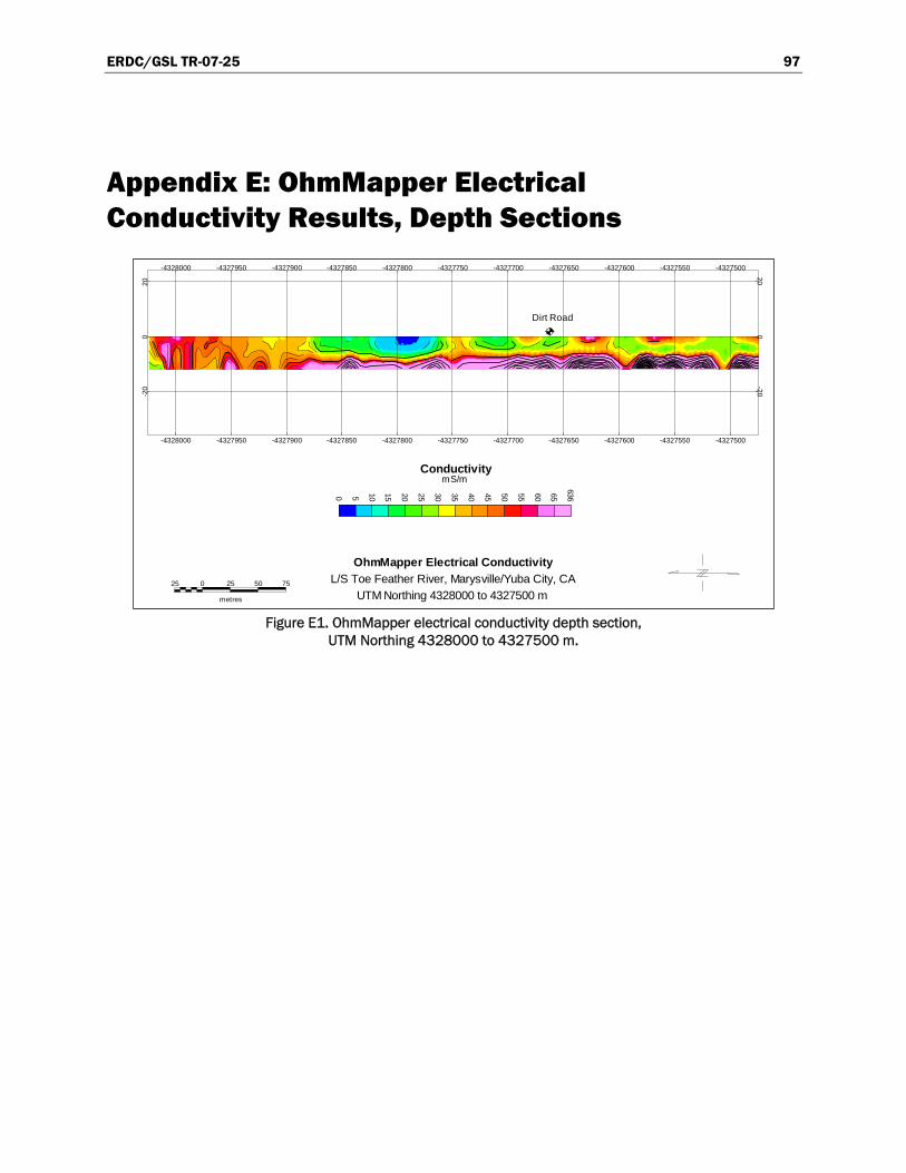
ERDC/GSL TR-07-25 97
Appendix E: OhmMapper Electrical Conductivity Results, Depth Sections
Figure E1. OhmMapper electrical conductivity depth section, UTM Northing 4328000 to 4327500 m.
25 0 25 50 75
metres
OhmMapper Electrical ConductivityL/S Toe Feather River, Marysville/Yuba City, CA
UTM Northing 4328000 to 4327500 m
0
6365 10 15 20 25 30 35 40 45 50 55 60 65
ConductivitymS/m
-20
020
-200
20
-4328000 -4327950 -4327900 -4327850 -4327800 -4327750 -4327700 -4327650 -4327600 -4327550 -4327500
-4328000 -4327950 -4327900 -4327850 -4327800 -4327750 -4327700 -4327650 -4327600 -4327550 -4327500
Dirt Road
0 5

ERDC/GSL TR-07-25 98
Figure E2. OhmMapper electrical conductivity depth section, UTM Northing 4327500 to 4327000 m.
Figure E3. OhmMapper electrical conductivity resistivity depth section, UTM Northing 4327000 to 4326500 m.
25 0 25 50 75
metres
OhmMapper Electrical ConductivityL/S Toe Feather River, Marysville/Yuba City, CA
UTM Northing 4327500 to 4327000 m
0
6365 10 15 20 25 30 35 40 45 50 55 60 65Conductivity
mS/m
-20
020
-200
20
-4327500 -4327450 -4327400 -4327350 -4327300 -4327250 -4327200 -4327150 -4327100 -4327050 -4327000
-4327500 -4327450 -4327400 -4327350 -4327300 -4327250 -4327200 -4327150 -4327100 -4327050 -4327000
Grassy RoadDirt Road Trash
0 50 5
25 0 25 50 75
metres
OhmMapper Electrical ConductivityL/S Toe Feather River, Marysville/Yuba City, CA
UTM Northing 4327000 to 4326500 m
0
6365 10 15 20 25 30 35 40 45 50 55 60 65
ConductivitymS/m
-20
020
-200
20
-4327000 -4326950 -4326900 -4326850 -4326800 -4326750 -4326700 -4326650 -4326600 -4326550 -4326500
-4327000 -4326950 -4326900 -4326850 -4326800 -4326750 -4326700 -4326650 -4326600 -4326550 -4326500
TrashRamp Trash

ERDC/GSL TR-07-25 99
Figure E4. OhmMapper electrical conductivity depth section, UTM Northing 4328000 to 4327500 m.
Figure E5. OhmMapper electrical conductivity depth section,
UTM Northing 4326000 to 4325500 m.
25 0 25 50 75
metres
OhmMapper Electrical ConductivityL/S Toe Feather River, Marysville/Yuba City, CA
UTM Northing 4326000 to 4325500 m
0
6365 10 15 20 25 30 35 40 45 50 55 60 65
ConductivitymS/m
-20
020
-200
20
-4326000 -4325950 -4325900 -4325850 -4325800 -4325750 -4325700 -4325650 -4325600 -4325550 -4325500
-4326000 -4325950 -4325900 -4325850 -4325800 -4325750 -4325700 -4325650 -4325600 -4325550 -4325500
Ella Road
High-Tension Power Line CrossingTrash Piles
Trash
25 0 25 50 75
metres
OhmMapper Electrical ConductivityL/S Toe Feather River, Marysville/Yuba City, CA
UTM Northing 4326500 to 4326000 m
0
6365 10 15 20 25 30 35 40 45 50 55 60 65Conductivity
mS/m
-20
020
-200
20
-4326500 -4326450 -4326400 -4326350 -4326300 -4326250 -4326200 -4326150 -4326100 -4326050 -4326000
-4326500 -4326450 -4326400 -4326350 -4326300 -4326250 -4326200 -4326150 -4326100 -4326050 -4326000
TrashRampTrash

ERDC/GSL TR-07-25 100
Figure E6. OhmMapper electrical conductivity depth section,
UTM Northing 4325500 to 4325000 m.
Figure E7. OhmMapper electrical conductivity depth section, UTM Northing 4325000 to 4324500 m.
25 0 25 50 75
metres
OhmMapper Electrical ConductivityL/S Toe Feather River, Marysville/Yuba City, CA
UTM Northing 4325500 to 4325000 m
0
6365 10 15 20 25 30 35 40 45 50 55 60 65Conductivity
mS/m
-20
020
-200
20
-4325500 -4325450 -4325400 -4325350 -4325300 -4325250 -4325200 -4325150 -4325100 -4325050 -4325000
-4325500 -4325450 -4325400 -4325350 -4325300 -4325250 -4325200 -4325150 -4325100 -4325050 -4325000
1.2 m Diameter Corrugated Steel Standpipe
25 0 25 50 75
metres
OhmMapper Electrical ConductivityL/S Toe Feather River, Marysville/Yuba City, CA
UTM Northing 4325000 to 4324500 m
0
6365 10 15 20 25 30 35 40 45 50 55 60 65
ConductivitymS/m
-20
020
-200
20
-4325000 -4324950 -4324900 -4324850 -4324800 -4324750 -4324700 -4324650 -4324600 -4324550 -4324500
-4325000 -4324950 -4324900 -4324850 -4324800 -4324750 -4324700 -4324650 -4324600 -4324550 -4324500
5 2
Dirt RoadRamp

ERDC/GSL TR-07-25 101
Figure E8. OhmMapper electrical conductivity depth section, UTM Northing 4324500 to 4324000 m.
Figure E9. OhmMapper electrical conductivity depth section, UTM Northing 4324000 to 4323500 m.
25 0 25 50 75
metres
OhmMapper Electrical ConductivityL/S Toe Feather River, Marysville/Yuba City, CA
UTM Northing 4324500 to 4324000 m
0
6365 10 15 20 25 30 35 40 45 50 55 60 65Conductivity
mS/m
-20
020
-200
20
-4324500 -4324450 -4324400 -4324350 -4324300 -4324250 -4324200 -4324150 -4324100 -4324050 -4324000
-4324500 -4324450 -4324400 -4324350 -4324300 -4324250 -4324200 -4324150 -4324100 -4324050 -4324000
Trash PileTrash PilesRamp
25 0 25 50 75
metres
OhmMapper Electrical ConductivityL/S Toe Feather River, Marysville/Yuba City, CA
UTM Northing 4324000 to 4323500 m
0
6365 10 15 20 25 30 35 40 45 50 55 60 65
ConductivitymS/m
-20
020
-200
20
-4324000 -4323950 -4323900 -4323850 -4323800 -4323750 -4323700 -4323650 -4323600 -4323550 -4323500
-4324000 -4323950 -4323900 -4323850 -4323800 -4323750 -4323700 -4323650 -4323600 -4323550 -4323500
RampWell
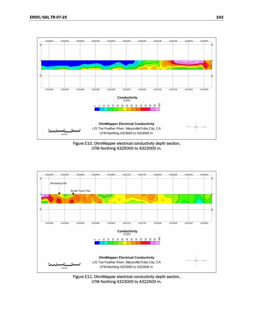
ERDC/GSL TR-07-25 102
Figure E10. OhmMapper electrical conductivity depth section, UTM Northing 4325000 to 4323000 m.
Figure E11. OhmMapper electrical conductivity depth section, UTM Northing 4323000 to 4322500 m.
25 0 25 50 75
metres
OhmMapper Electrical ConductivityL/S Toe Feather River, Marysville/Yuba City, CA
UTM Northing 4323500 to 4323000 m
0
6365 10 15 20 25 30 35 40 45 50 55 60 65Conductivity
mS/m
-20
020
-200
20
-4323500 -4323450 -4323400 -4323350 -4323300 -4323250 -4323200 -4323150 -4323100 -4323050 -4323000
-4323500 -4323450 -4323400 -4323350 -4323300 -4323250 -4323200 -4323150 -4323100 -4323050 -4323000
5 2
05
25 0 25 50 75
metres
OhmMapper Electrical ConductivityL/S Toe Feather River, Marysville/Yuba City, CA
UTM Northing 4323000 to 4322500 m
0
6365 10 15 20 25 30 35 40 45 50 55 60 65
ConductivitymS/m
-20
020
-200
20
-4323000 -4322950 -4322900 -4322850 -4322800 -4322750 -4322700 -4322650 -4322600 -4322550 -4322500
-4323000 -4322950 -4322900 -4322850 -4322800 -4322750 -4322700 -4322650 -4322600 -4322550 -4322500
Small Trash Pile
Broadway Rd.
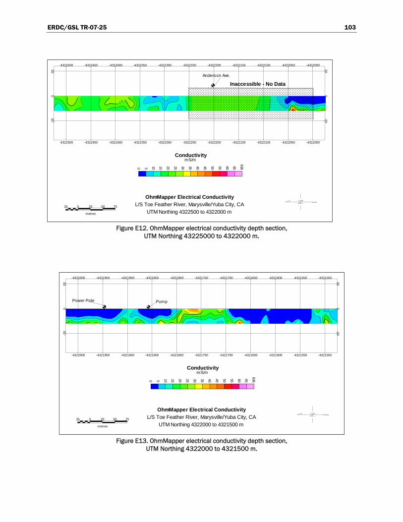
ERDC/GSL TR-07-25 103
Figure E12. OhmMapper electrical conductivity depth section, UTM Northing 43225000 to 4322000 m.
Figure E13. OhmMapper electrical conductivity depth section, UTM Northing 4322000 to 4321500 m.
25 0 25 50 75
metres
OhmMapper Electrical ConductivityL/S Toe Feather River, Marysville/Yuba City, CA
UTM Northing 4322500 to 4322000 m
0
6365 10 15 20 25 30 35 40 45 50 55 60 65
ConductivitymS/m
-20
020
-200
20
-4322500 -4322450 -4322400 -4322350 -4322300 -4322250 -4322200 -4322150 -4322100 -4322050 -4322000
-4322500 -4322450 -4322400 -4322350 -4322300 -4322250 -4322200 -4322150 -4322100 -4322050 -4322000
Inaccessible - No DataAnderson Ave.
52
25 0 25 50 75
metres
OhmMapper Electrical ConductivityL/S Toe Feather River, Marysville/Yuba City, CA
UTM Northing 4322000 to 4321500 m
0
6365 10 15 20 25 30 35 40 45 50 55 60 65
ConductivitymS/m
-20
020
-200
20
-4322000 -4321950 -4321900 -4321850 -4321800 -4321750 -4321700 -4321650 -4321600 -4321550 -4321500
-4322000 -4321950 -4321900 -4321850 -4321800 -4321750 -4321700 -4321650 -4321600 -4321550 -4321500
PumpPower Pole

ERDC/GSL TR-07-25 104
Figure E14. OhmMapper electrical conductivity depth section, UTM Northing 4321500 to 4321000 m.
Figure E15. OhmMapper electrical conductivity depth section, UTM Northing 4321000 to 4320500 m.
25 0 25 50 75
metres
OhmMapper Electrical ConductivityL/S Toe Feather River, Marysville/Yuba City, CA
UTM Northing 4321500 to 4321000 m
0
6365 10 15 20 25 30 35 40 45 50 55 60 65Conductivity
mS/m
-20
020
-200
20
-4321500 -4321450 -4321400 -4321350 -4321300 -4321250 -4321200 -4321150 -4321100 -4321050 -4321000
-4321500 -4321450 -4321400 -4321350 -4321300 -4321250 -4321200 -4321150 -4321100 -4321050 -4321000
Trash PileWater Pump
Country Club Lane
Water Pump
25 0 25 50 75
metres
OhmMapper Electrical ConductivityL/S Toe Feather River, Marysville/Yuba City, CA
UTM Northing 4321000 to 4320500 m
0
6365 10 15 20 25 30 35 40 45 50 55 60 65
ConductivitymS/m
-20
020
-200
20
-4321000 -4320950 -4320900 -4320850 -4320800 -4320750 -4320700 -4320650 -4320600 -4320550 -4320500
-4321000 -4320950 -4320900 -4320850 -4320800 -4320750 -4320700 -4320650 -4320600 -4320550 -4320500
Inaccessible Area - No Data
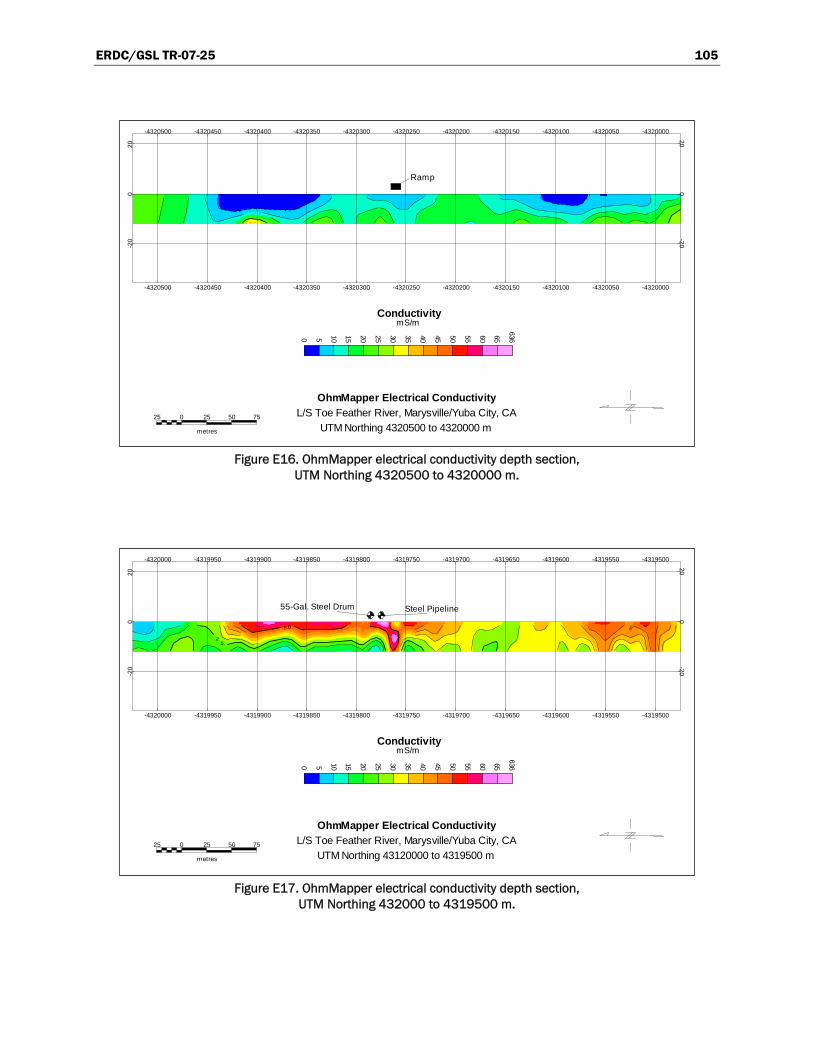
ERDC/GSL TR-07-25 105
Figure E16. OhmMapper electrical conductivity depth section, UTM Northing 4320500 to 4320000 m.
Figure E17. OhmMapper electrical conductivity depth section, UTM Northing 432000 to 4319500 m.
25 0 25 50 75
metres
OhmMapper Electrical ConductivityL/S Toe Feather River, Marysville/Yuba City, CA
UTM Northing 4320500 to 4320000 m
0
6365 10 15 20 25 30 35 40 45 50 55 60 65Conductivity
mS/m
-20
020
-200
20
-4320500 -4320450 -4320400 -4320350 -4320300 -4320250 -4320200 -4320150 -4320100 -4320050 -4320000
-4320500 -4320450 -4320400 -4320350 -4320300 -4320250 -4320200 -4320150 -4320100 -4320050 -4320000
Ramp
25 0 25 50 75
metres
OhmMapper Electrical ConductivityL/S Toe Feather River, Marysville/Yuba City, CA
UTM Northing 43120000 to 4319500 m
0
6365 10 15 20 25 30 35 40 45 50 55 60 65
ConductivitymS/m
-20
020
-200
20
-4320000 -4319950 -4319900 -4319850 -4319800 -4319750 -4319700 -4319650 -4319600 -4319550 -4319500
-4320000 -4319950 -4319900 -4319850 -4319800 -4319750 -4319700 -4319650 -4319600 -4319550 -4319500
Steel Pipeline55-Gal. Steel Drum
52
05

ERDC/GSL TR-07-25 106
Figure E18. OhmMapper electrical conductivity depth section, UTM Northing 4319500 to 4319000 m.
25 0 25 50 75
metres
OhmMapper Electrical ConductivityL/S Toe Feather River, Marysville/Yuba City, CA
UTM Northing 4319500 to 4319000 m
0
6365 10 15 20 25 30 35 40 45 50 55 60 65Conductivity
mS/m
-20
020
-200
20
-4319500 -4319450 -4319400 -4319350 -4319300 -4319250 -4319200 -4319150 -4319100 -4319050 -4319000
-4319500 -4319450 -4319400 -4319350 -4319300 -4319250 -4319200 -4319150 -4319100 -4319050 -4319000
N End of Fence
5 0

ERDC/GSL TR-07-25 107
Appendix F: SARIS Electrical Conductivity Results, Depth Sections
25 0 25 50 75
(meters)
Scintrex Electrical ConductivityL/S Toe Feather River, Marysville/Yuba City, CA
UTM Northing 4328000 to 4327500
-3 1755 10 15 20 25 30 35 40 45 50 55 60 65
ConductivitymS/m
-5-5
-4328000 -4327950 -4327900 -4327850 -4327800 -4327750 -4327700 -4327650 -4327600 -4327550 -4327500
-4328000 -4327950 -4327900 -4327850 -4327800 -4327750 -4327700 -4327650 -4327600 -4327550 -4327500Road
Figure F1. SARIS electrical conductivity depth section,
UTM Northing 4327750 to 4327500 m.
25 0 25 50 75
(meters)
Scintrex Electrical ConductivityL/S Toe Feather River, Marysville/Yuba City, CA
UTM Northing 4327500 to 4327000
-3 1755 10 15 20 25 30 35 40 45 50 55 60 65
ConductivitymS/m
-5-5
-4327500 -4327450 -4327400 -4327350 -4327300 -4327250 -4327200 -4327150 -4327100 -4327050 -4327000
-4327500 -4327450 -4327400 -4327350 -4327300 -4327250 -4327200 -4327150 -4327100 -4327050 -4327000
Road Trash Grassy Road
Figure F2. SARIS electrical conductivity depth section,
UTM Northing 4327500 to 4327000 m.
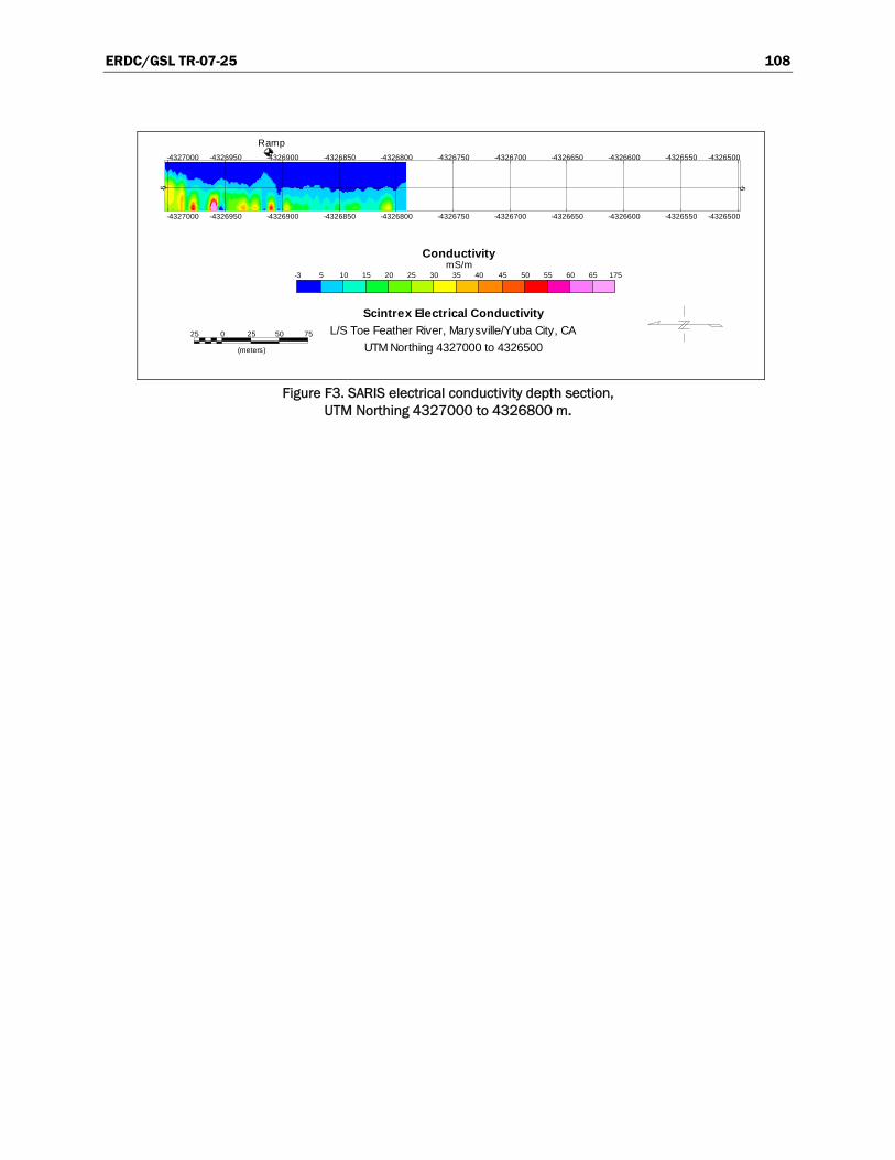
ERDC/GSL TR-07-25 108
25 0 25 50 75
(meters)
Scintrex Electrical ConductivityL/S Toe Feather River, Marysville/Yuba City, CA
UTM Northing 4327000 to 4326500
-3 1755 10 15 20 25 30 35 40 45 50 55 60 65
ConductivitymS/m
-5-5
-4327000 -4326950 -4326900 -4326850 -4326800 -4326750 -4326700 -4326650 -4326600 -4326550 -4326500
-4327000 -4326950 -4326900 -4326850 -4326800 -4326750 -4326700 -4326650 -4326600 -4326550 -4326500
Ramp
Figure F3. SARIS electrical conductivity depth section,
UTM Northing 4327000 to 4326800 m.

REPORT DOCUMENTATION PAGE Form Approved
OMB No. 0704-0188 Public reporting burden for this collection of information is estimated to average 1 hour per response, including the time for reviewing instructions, searching existing data sources, gathering and maintaining the data needed, and completing and reviewing this collection of information. Send comments regarding this burden estimate or any other aspect of this collection of information, including suggestions for reducing this burden to Department of Defense, Washington Headquarters Services, Directorate for Information Operations and Reports (0704-0188), 1215 Jefferson Davis Highway, Suite 1204, Arlington, VA 22202-4302. Respondents should be aware that notwithstanding any other provision of law, no person shall be subject to any penalty for failing to comply with a collection of information if it does not display a currently valid OMB control number. PLEASE DO NOT RETURN YOUR FORM TO THE ABOVE ADDRESS.
1. REPORT DATE (DD-MM-YYYY) September 2007
2. REPORT TYPE Final report
3. DATES COVERED (From - To)
5a. CONTRACT NUMBER
5b. GRANT NUMBER
4. TITLE AND SUBTITLE
Geophysical Surveys for Assessing Levee Foundation Conditions, Feather River Levees, Marysville/Yuba City, California
5c. PROGRAM ELEMENT NUMBER
5d. PROJECT NUMBER
5e. TASK NUMBER
6. AUTHOR(S) José L. Llopis and Janet E. Simms
5f. WORK UNIT NUMBER
7. PERFORMING ORGANIZATION NAME(S) AND ADDRESS(ES) 8. PERFORMING ORGANIZATION REPORT NUMBER
U.S. Army Engineer Research and Development Center Geotechnical and Structures Laboratory 3909 Halls Ferry Road Vicksburg, MS 39180-6199
ERDC/GSL TR-07-25
9. SPONSORING / MONITORING AGENCY NAME(S) AND ADDRESS(ES) 10. SPONSOR/MONITOR’S ACRONYM(S)
11. SPONSOR/MONITOR’S REPORT NUMBER(S)
Headquarters, U.S. Army Corps of Engineers Washington, DC 20314-1000
12. DISTRIBUTION / AVAILABILITY STATEMENT Approved for public release; distribution is unlimited.
13. SUPPLEMENTARY NOTES
14. ABSTRACT
Effective flood and coastal storm emergency response depends on the ability of emergency managers to obtain information on the condition of flood-damage reduction structures in near real-time. This report describes the results of a geophysical study performed to determine the potential for geophysical methods to provide supplemental geologic data between existing soil borings in a rapid fashion in an area of complex geology. The geophysical study was conducted along 10 km of landside levee toe adjacent to the Feather River, approximately 5 km south of Marysville/Yuba City, CA. Electromagnetic induction, capacitively coupled electrical resistivity, and direct current electrical resistivity survey methods were used to conduct the geophysical study. Survey results were used to classify soil type to depths of approximately 60 m.
15. SUBJECT TERMS Electrical resistivity Electromagnetic induction
Feather River Feather River levees Geophysics
Levee assessment Marysville, CA Yuba City, CA
16. SECURITY CLASSIFICATION OF: 17. LIMITATION OF ABSTRACT
18. NUMBER OF PAGES
19a. NAME OF RESPONSIBLE PERSON
a. REPORT
UNCLASSIFIED
b. ABSTRACT
UNCLASSIFIED
c. THIS PAGE
UNCLASSIFIED 115 19b. TELEPHONE NUMBER (include area code)
Standard Form 298 (Rev. 8-98) Prescribed by ANSI Std. 239.18