environmental regulation and modelling of cassava canopy conductance under drying root-zone soil...

METEOROLOGICAL APPLICATIONSMeteorol. Appl. 14: 245–252 (2007)Published online 1 August 2007 in Wiley InterScience(www.interscience.wiley.com) DOI: 10.1002/met.24

Environmental regulation and modelling of cassava canopyconductance under drying root-zone soil water

Philip G. Oguntundea,b* and Michael O. Alatisea

a Department of Agricultural Engineering, Federal University of Technology, Akure, Nigeriab Department of Water Management, Faculty of Civil Engineering and Geosciences, Delft University of Technology, Netherlands

ABSTRACT: Sap flow was measured, with Granier-type sensors, in a crop of field-grown water-stressed cassava (Manihotesculenta Crantz) in Ghana, West Africa. The main objective of this study was to examine the environmental controlof canopy conductance (gc) with a view to modelling the stomatal control of water transport under water-stressedcondition. Weather variables measured concurrently with sap flow were: air temperature (Ta), relative humidity (RH ),wind speed (u) and solar radiation (Rs). Relationship between canopy conductance (gc) and vapour pressure deficit(Dε) was curvilinear while no specific pattern was observed with Rs . Average diurnal gc decreased from 3.0 ± 0.6 to0.7 ± 0.4 mm s−1 between 0730 and 2000 h local time (= GMT) each day. A Jarvis-type model, based on a set ofenvironmental control functions, was parameterized for the cassava crop in this study. Model results demonstrated that gc

was estimated with a high degree of accuracy based on Rs, Ta , and Dε (r2 = 0.92;F = 809.2;P < 0.0001). Dε explainedabout 90% (F = 2129.7;P < 0.0001) of the variations observed in gc, whereas both Rs and Ta contributed about 2% of theexplained variance in gc. The aerodynamic conductance (ga) was very high compared to gc, leading to a daily average ratioga/gc > 100 and a decoupling factor< 0.1. Cross-validation analysis revealed a consistent good performance (r2 > 0.85)of the gc model with Dε as the only independent environmental variable. Copyright 2007 Royal Meteorological Society

KEY WORDS cassava; sap flow; drying root-zone; canopy conductance; regulation and modelling

1. Introduction

Cassava (Manihot esculenta Crantz), a short-lived woodyperennial tropical shrub growing between 1.0 and 3.5 mtall, is known to be highly productive under favourableconditions and produce reasonably well under adverseconditions where other crops fail. Cassava is Africa’ssecond most important food staple, after maize, in termsof calories consumed (Nweke, 2004). Africa accountsfor more than half the world’s cassava production(IITA, 1997). However, most of the increases in cas-sava production have been due to cropland expansion,rather than increases in yield per hectare, as the areaunder production has increased by 70% in the last twodecades (Hillocks, 2002). Presently, as cassava culti-vation is expanding into non-traditional areas such assemi-arid regions of sub-saharan Africa (El-Sharkawy,1993), efforts to develop high yielding and drought tol-erant varieties are being advocated (El-Sharkawy, 1993,2006; Hillocks, 2002; Nweke, 2004). For food securityand environmental sustainability, future increase in cas-sava production should be based on alternative optionsother than expansion of cultivated lands as currently prac-tised. Hence, the possibility of increasing production per

* Correspondence to: Philip G. Oguntunde, Department of AgriculturalEngineering, Federal University of Technology, Akure, Nigeria.E-mail: [email protected]

unit land area under cultivation using supplemental irri-gation or enhancing rainwater use efficiency should beexploited. However, for the purpose of precise waterapplications, it is essential to understand fully cassava’sresponse to water deficit as well as to define water useand its regulations under different field conditions.

Several studies reporting the response of cassava towater stress have been carried out on plants grown inlarge pots in the open (El-Sharkawy and Cock, 1984;El-Sharkawy et al., 1984), under a controlled environ-ment such as screen or glass house (Alves and Setter,2000) or under field conditions where water exclusion isartificial by covering the soil with plastic sheets (Con-nor et al., 1981; Connor and Palta, 1981; El-Sharkawyand Cock, 1987; El-Sharkawy et al., 1992; El-Sharkawyand Cadavid, 2002). The results of such experimentsneed confirmation and calibration for the natural envi-ronmental conditions under which plants develop. DeTafur et al. (1997) found that both upper canopy leafconductance and photosynthetic rate, as measured with aportable infrared gas analyser during the dry period, ofseveral cassava clones field-grown in seasonally dry andsemi-arid locations in northern Colombia were highestat early morning and declined rapidly over the day asair humidity decreased from morning to mid-afternoon.Similarly, El-Sharkawy (1990) reported that leaf conduc-tance and transpiration rate, as measured with a porom-eter during the dry period, of field-grown cassava in

Copyright 2007 Royal Meteorological Society

246 P. G. OGUNTUNDE AND M. O. ALATISE

wet soil at the Colombian Eastern Plains (Los LlanosOrientales) were negatively correlated with vapour pres-sure deficit (Dε) without measurable changes in bulkleaf water potential. Wind velocity of about 4 m s−1

also resulted in a significant decrease in leaf conduc-tance because of the removal of the humid boundary layerover leaves, hence increasing leaf-to-air Dε. El-Sharkawy(2005, 2006) recently reviewed and discussed the impor-tance of field research under natural conditions to avoidplant acclimation/adaptation problems and recommendedthat data obtained under controlled conditions should becalibrated in the field, particularly when such data areintended to be extrapolated to field conditions or usedfor crop/environment modelling.

Previous studies have shown that cassava respondsto drought by closing its stomata apparatus to reducetranspiration, which acts to protect leaf tissues from tur-gor loss and desiccation (Connor and Palta, 1981; El-Sharkawy and Cock, 1984; El-Sharkawy et al., 1992;El-Sharkawy, 1993; Alves and Setter, 2000). Reduc-tions in apparent photosynthesis and leaf transpirationhave also been attributed to decreases in leaf conduc-tance in response to increasing humidity deficit underwell-watered and stressed conditions in potted plantsgrown outdoors as well as in field-grown crops (El-Sharkawy and Cock, 1984; El-Sharkawy, 1990, 2006;De Tafur et al., 1997). The need for field studies on theresponse of different cassava cultivars to varying evap-orative demand, particularly under limited soil water,has been proposed for identification of parental mate-rials for developing drought-tolerant improved cultivars(El-Sharkawy et al., 1984).

Measurements of single leaf conductance in most of theabove studies were made with porometers and/or withinfrared gas analysers that monitor both CO2 and H2Oexchanges, which are often costly, time consuming, andpresent limitations for scaling to plant canopy and con-tinuous real-time monitoring (Green and McNaughton,1997; Lu et al., 2003). Alternatively, in the present study,weather data were combined with sap flow measure-ment techniques to provide a low-cost option to studythe effects of changing atmospheric conditions on canopyphysiological response on a continuous basis. Therefore,the objective of this study was to examine the environ-mental control of cassava canopy conductance (gc) with aview to modelling the stomatal control of water transportunder water-stressed conditions.

2. Methods and data analysis

2.1. Study site

The experiment was conducted in a 1.2 ha field of11-months-old cassava field with a plant density of12 500 plants ha−1, located in the Kotokosu watershed15 km east of Ejura, Ghana (07°20′N, 01°16′W, 210 mabove mean sea level). The cultivar is the IITA’s newhigh-yielding Tropical Manioc Selection (TMS30572)variety with pest and disease resistant ability (O O Aina,

IITA, Ibadan: personal communication), popular withfarmers in Nigeria and Ghana, the two leading cassavaproducing countries in West Africa (Nweke, 2004). Theleaf area index was measured as 3.2 ± 0.6 m2 m−2 usinga SunScan canopy analysis system (Delta-T Devices,Cambridge, UK). Average trunk diameter within the48 m2 plot was 3.4 cm. During the study the field wasmainly free of weeds. The climate is tropical monsooncharacterized with distinct wet (April–October) and dry(November–March) seasons. The 20-year (1973–1992)annual rainfall average is 1264 mm with an annual meanair temperature of 26.6 °C (Oguntunde et al., 2004).

2.2. Weather and soil moisture measurements

Weather variables, such as incoming solar radiation (SP-LITE pyranometer, Kipp and Zonen, Delft), air temper-ature (50Y Temperature probe, Vaisala, Finland), rela-tive humidity (50Y Relative Humidity, Vaisala, Finland),wind speed and direction (A100R Anemometer, VectorInstruments, UK), were sampled every ten seconds andrecorded as ten-min averages with a CR10X datalogger(Campbell Scientific, Inc., USA). Incoming and reflectedsolar radiation was measured with a simple albedome-ter constructed from two pyranometers (model SP LITE,Kipp and Zonen, Delft, Netherlands) horizontally posi-tioned 1.5 m above the plant canopy for two days. Soilmoisture was routinely measured in three access tubeslocated in the vicinity of the cassava field. A profile probetype PR1/6 (Delta-T Devices, Cambridge, England) wasused to monitor the soil water content at six differentdepths to 100 cm.

2.3. Sap flow measurements and analysis

Sap flow was measured within a 6 × 8 m2 plot,located in the centre of the field to avoid possibleedge effects, using the temperature difference methodof Granier (1987). Two cylindrical probes, 2 mm indiameter, were implanted in the cassava trunks withpreviously installed aluminium tubes, separated verticallyby 10 cm. The probes were installed on the north side ofeach plant, to minimize direct heating from sunshine, andthen shielded with aluminium foil against rainfall, fog,dew and incident radiation. The downstream probe wascontinuously heated with a constant power source, whilethe unheated upstream probe served as a temperaturereference. The dissipation of heat from the upstreamheated needle increased with increasing sap flow rate.During conditions of zero sap flow, such as nighttime,the temperature difference between the lower and theupper probes represented the steady state temperaturedifference caused by the dissipation of heat into non-transporting sapwood. A copper-constantan thermocouplemeasured the temperature difference between the heatedupper needle and unheated lower reference needle. Sapvelocity (V , cm s−1) was computed through an empiricalrelationship validated and confirmed for many species

Copyright 2007 Royal Meteorological Society Meteorol. Appl. 14: 245–252 (2007)DOI: 10.1002/met

ENVIRONMENTAL REGULATION OF CASSAVA CANOPY CONDUCTANCE 247

(Granier, 1987; Braun and Schmid, 1999) as:

V = 0.0119(

�Tmax − �T

�T

)1.231

(1)

where �T is the temperature difference between the twoprobes and �T max is the baseline (maximum) temperaturedifference for the dataset of the day. Three representativestems were selected for sap flow gauging based onstratification of stem sizes (within the plot) into threeclasses. Plot transpiration (Ec), based on sap velocityof the monitored trees, was estimated as the product ofweighted flow velocity and the ratio of sapwood area (As)and the ground area (Ag):

Ec = VAs

Ag

(2)

Sap flow, sampled at 10-min intervals, was recordedfor ten consecutive rainless days between 15 and 24December 2002.

2.4. Canopy conductance estimation and modelling

The analysis of canopy conductance was made using thePenman–Monteith equation, which is one of the mostcommonly used equation (for more information on soil-water-plant-atmosphere modelling see Ritchie and John-son, 1990), to describe the process of canopy transpirationby integrating plant physiology and environmental fac-tors. The equation is given by:

λEc = �A + ρaCpDεga

� + γ [1 + ga/gc](3)

where gc (m s−1) is the canopy conductance, � (kPa K−1)is the rate of change of vapour pressure with temperature,γ (kPa K−1) is the psychometric constant, ρa (kg m−3)is the density of dry air, Cp is the specific heat capacityof the air (J kg−1 K−1), Dε is the vapour pressure deficit(kPa), ga is the aerodynamic conductance (m s−1), λ isthe latent heat of water vaporization (J kg−1), Ec is thecanopy transpiration (kg m−2 s−1) and A is the avail-able energy at the canopy level (W m−2). The gc wasestimated by inverting Equation (3) and substituting sapflow-based transpiration values. This represents the bulkor integrated behaviour of the leaf stomata conductance(Stewart, 1988), and is the key crop parameter reflect-ing its physiological response to changing atmosphericconditions. Rearranging Equation (3) gives:

gc = γλEcga

�A + ρaCpDεga − λ(� + γ )Ec

(4)

where the ga has been derived, following the formulationof Thom and Oliver (1977), as:

ga = 4.72{ln(z − d/z0)}2

1 + 0.54u(5)

where u is the wind speed (m s−1) at the z wind mea-surement height (m), d (m) is the zero plane displacementestimated as d = 0.67hc, with hc as the mean crop height(m); and z0 is the roughness length taken as 0.1hc. Bytaking the limit of infinite ga of the Penman–Monteithequation (Monteith and Unsworth, 1990; Bosveld andBouten, 2001), a simplified form of Equation (4) couldbe written as:

gc = γλEc

ρaCpDε

(6)

Equation (6) has been shown to be valid especiallywhen the vegetation canopy is well coupled with theatmosphere, with Dε mainly controlling the canopyprocesses resulting to the decoupling factor of ≤ 0.2(Granier et al., 1996; Bosveld and Bouten, 2001). Equa-tion (6) was tested against Equation (4) to assess howfar this simplified approximation works under a water-stressed condition.

Studies have shown that gc depends mainly on fac-tors such as Rs, Ta, Dε and soil moisture (Jarvis, 1976;Stewart, 1988). In the present study, the approach basedon an analytical model of gc proposed by Jarvis (1976),was parameterized. This model has been extensivelyused in many soil-vegetation-atmosphere-transfer (SVAT )schemes and is based on semi-empirical functions ofstomatal control (Wright et al., 1995). Stomatal conduc-tance is often modelled as a product of response functions(f ) that have values between 0 and 1 (0 ≤ f ≤ 1). Thegc is assumed to be determined by Dε, Ta , and Rs accord-ing to

gc = k1f (Dε)f (Ta)f (Rs) (7)

where k1, the first model parameter, represent maximumstomatal conductance. Other control functions are:

f (Dε) = exp(−k2Dε) (8)

f (Ta) = (Ta − TL)(TH − Ta)t

(k3 − TL)(TH − k3)t (9)

t = TH − k3

k3 − TL

(10)

f (Rs) = Rs

1000

1000 + k4

Rs + k4(11)

where TL and TH are the lower and upper tempera-ture limit to transpiration fixed between 0 and 45 °C,respectively (Wright et al., 1995). Parameters k1 – k4

were optimized using the Levenberg–Marquardt algo-rithm (Marquardt, 1963). To avoid uncertainties of usingthe nighttime measurements, measurements for the day-time (0800–1700 h) were used as modelling inputs. Formodel optimization and cross-validation, the data weredivided into two equal sets: Dataset A consisted of allthe odd days of measurement, while Dataset B consistedof all the even days. Dataset B was used to validate the



model fitted on Dataset A and vice versa. This type ofvalidation procedure has been described as robust andconsistent (Stewart, 1988; Lu et al., 2003).

3. Results

3.1. Environmental conditions, sap flow and canopyconductance

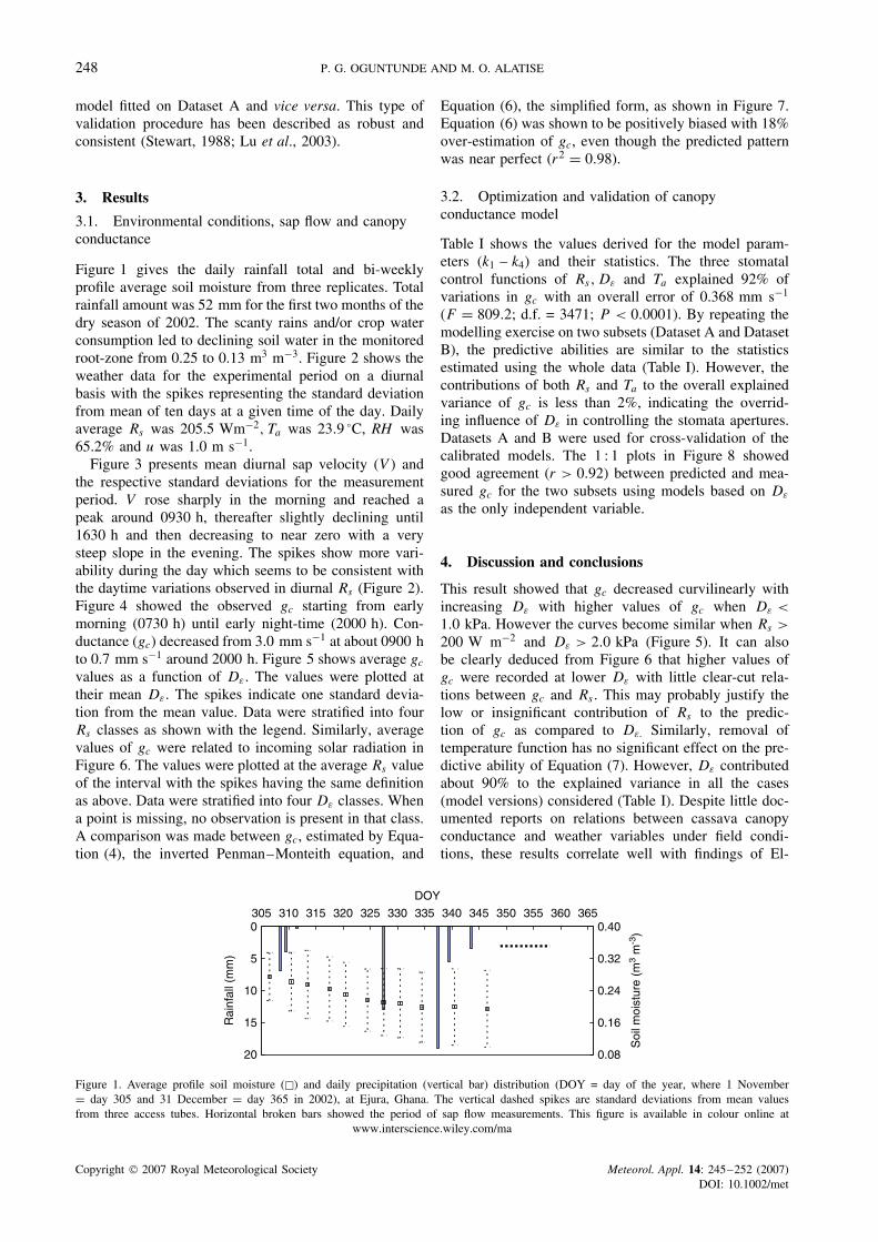
Figure 1 gives the daily rainfall total and bi-weeklyprofile average soil moisture from three replicates. Totalrainfall amount was 52 mm for the first two months of thedry season of 2002. The scanty rains and/or crop waterconsumption led to declining soil water in the monitoredroot-zone from 0.25 to 0.13 m3 m−3. Figure 2 shows theweather data for the experimental period on a diurnalbasis with the spikes representing the standard deviationfrom mean of ten days at a given time of the day. Dailyaverage Rs was 205.5 Wm−2, Ta was 23.9 °C, RH was65.2% and u was 1.0 m s−1.

Figure 3 presents mean diurnal sap velocity (V ) andthe respective standard deviations for the measurementperiod. V rose sharply in the morning and reached apeak around 0930 h, thereafter slightly declining until1630 h and then decreasing to near zero with a verysteep slope in the evening. The spikes show more vari-ability during the day which seems to be consistent withthe daytime variations observed in diurnal Rs (Figure 2).Figure 4 showed the observed gc starting from earlymorning (0730 h) until early night-time (2000 h). Con-ductance (gc) decreased from 3.0 mm s−1 at about 0900 hto 0.7 mm s−1 around 2000 h. Figure 5 shows average gc

values as a function of Dε. The values were plotted attheir mean Dε. The spikes indicate one standard devia-tion from the mean value. Data were stratified into fourRs classes as shown with the legend. Similarly, averagevalues of gc were related to incoming solar radiation inFigure 6. The values were plotted at the average Rs valueof the interval with the spikes having the same definitionas above. Data were stratified into four Dε classes. Whena point is missing, no observation is present in that class.A comparison was made between gc, estimated by Equa-tion (4), the inverted Penman–Monteith equation, and

Equation (6), the simplified form, as shown in Figure 7.Equation (6) was shown to be positively biased with 18%over-estimation of gc, even though the predicted patternwas near perfect (r2 = 0.98).

3.2. Optimization and validation of canopyconductance model

Table I shows the values derived for the model param-eters (k1 – k4) and their statistics. The three stomatalcontrol functions of Rs, Dε and Ta explained 92% ofvariations in gc with an overall error of 0.368 mm s−1

(F = 809.2; d.f. = 3471; P < 0.0001). By repeating themodelling exercise on two subsets (Dataset A and DatasetB), the predictive abilities are similar to the statisticsestimated using the whole data (Table I). However, thecontributions of both Rs and Ta to the overall explainedvariance of gc is less than 2%, indicating the overrid-ing influence of Dε in controlling the stomata apertures.Datasets A and B were used for cross-validation of thecalibrated models. The 1 : 1 plots in Figure 8 showedgood agreement (r > 0.92) between predicted and mea-sured gc for the two subsets using models based on Dε

as the only independent variable.

4. Discussion and conclusions

This result showed that gc decreased curvilinearly withincreasing Dε with higher values of gc when Dε <

1.0 kPa. However the curves become similar when Rs >

200 W m−2 and Dε > 2.0 kPa (Figure 5). It can alsobe clearly deduced from Figure 6 that higher values ofgc were recorded at lower Dε with little clear-cut rela-tions between gc and Rs . This may probably justify thelow or insignificant contribution of Rs to the predic-tion of gc as compared to Dε. Similarly, removal oftemperature function has no significant effect on the pre-dictive ability of Equation (7). However, Dε contributedabout 90% to the explained variance in all the cases(model versions) considered (Table I). Despite little doc-umented reports on relations between cassava canopyconductance and weather variables under field condi-tions, these results correlate well with findings of El-

0

5

10

15

20

305 310 315 320 325 330 335 340 345 350 355 360 365

DOY

Rai

nfal

l (m

m)

0.08

0.16

0.24

0.32

0.40

Soi

l moi

stur

e (m

3 m

-3)

Figure 1. Average profile soil moisture (�) and daily precipitation (vertical bar) distribution (DOY = day of the year, where 1 November= day 305 and 31 December = day 365 in 2002), at Ejura, Ghana. The vertical dashed spikes are standard deviations from mean valuesfrom three access tubes. Horizontal broken bars showed the period of sap flow measurements. This figure is available in colour online at

www.interscience.wiley.com/ma



(a)

0.0

200.0

400.0

600.0

800.0

1000.0

0.0 4.0 8.0 12.0 16.0 20.0 24.0

Time of day (h)

0.0 4.0 8.0 12.0 16.0 20.0 24.0

Time of day (h)

0.0 4.0 8.0 12.0 16.0 20.0 24.0

Time of day (h)

Rs

(W m

-2)

(b)

15.0

20.0

25.0

30.0

35.0

0.0 4.0 8.0 12.0 16.0 20.0 24.0

Time of day (h)

Ta

(°C

)

(c)

20.0

40.0

60.0

80.0

100.0

120.0

RH

(%

)

(d)

0.0

1.0

2.0

3.0

U (

m s

-1)

Figure 2. Mean diurnal pattern of (a) solar radiation (Rs ), (b) air temperature (Ta), (c) relative humidity (RH ), and (d) wind speed (u) duringthe ten days of sap flow measurement at Ejura, Ghana. The vertical spikes are standard deviations from mean values of respective time of the

day. This figure is available in colour online at www.interscience.wiley.com/ma

0.0

4.0

8.0

12.0

16.0

0.0 4.0 8.0 12.0 16.0 20.0 24.0

Time of day (h)

Sap

vel

ocity

(cm

h-1

)

Figure 3. Mean diurnal pattern of cassava sap velocity between DOY349 and DOY 358 in 2002. The vertical spikes are standard deviationsfrom mean values of respective time of the day. This figure is available

in colour online at www.interscience.wiley.com/ma

0.0

1.0

2.0

3.0

4.0

7.0 9.0 11.0 13.0 15.0 17.0 19.0 21.0

Time of day (h)

g c (

mm

s-1

)

Figure 4. Mean diurnal pattern of canopy conductance (gc) betweenDOY 349 and 358 in 2002. The vertical spikes are standard devi-ations from mean values of respective time of the day between7 : 30 and 20 : 00 h. This figure is available in colour online at

www.interscience.wiley.com/ma

0.0

1.5

3.0

4.5

0.0 1.0 2.0 3.0 4.0

De (kPa)

g c (

mm

s-1

)

Figure 5. Effect of vapour pressure deficit (Dε) on canopy conductance(gc) under different classes of solar radiation (Rs < 200 W m−2

[°], Rs = 200–400 W m−2 [�], Rs = 400–600 W m−2 [x], Rs >

600 W m−2 [�]). Point for a class is drawn at the average value ofDε . The error bar for a class is the standard deviation from the mean

of that class.

Sharkawy and Cock (1984), which were conducted ina controlled environment and at constant but high pho-tosynthetic photon flux density. The diurnal pattern ofcanopy conductance (gc) was similar to single leaf con-ductance of field-grown cassava reported by Connor andPalta (1981) and Cock et al. (1985). A sharp decline ofcanopy conductance (gc) in response to increasing Dε

indicates high sensitivity of cassava leaves to chang-ing atmospheric humidity and hence the regulation ofits transpiration at the canopy level. Connor and Palta(1981) also reported the existence of significant correla-tion between cassava leaf conductance, as measured withporometers, and leaf-air vapour pressure deficit, with the



0.0

1.5

3.0

4.5

0.0 200.0 400.0 600.0 800.0

Rs (W m-2)

g c (

mm

s-1

)

Figure 6. Observed canopy conductance (gc) as a function of solarradiation (Rs) under different classes of vapour pressure deficit (Dε < 1kPa [°], Dε = 1–2 kPa [�], Dε = 2–3 kPa [x], Dε > 3 kPa [�]).Point for a class is drawn at the average value of Rs . The error bar for

a class is the standard deviation from the mean of that class.

highest correlation coefficients in the vigorous cultivarM Mex 59. In comparison with diverse species underwell water conditions, the degree of stomatal response toDε, with a strong linear decrease, was highest in cassava

0.0

1.0

2.0

3.0

4.0

5.0

6.0

0.0 1.0 2.0 3.0 4.0 5.0 6.0

gc, mm s-1 (Eq 4)

g c, m

m s

-1 (

Eq

6)

Figure 7. A simple relationship (y = 1.18x, r2 = 0.98) betweencanopy conductance (gc) estimated with Equation 4, the invertedPenman–Monteith equation, and with Equation 6, the simplified

approximation.

(El-Sharkawy et al., 1984). The curvilinear patternobserved in this study could be attributed to water short-age condition. This type of stomata response to Dε helpscassava to avoid excessive water loss at high Dε andbecomes important strategy to survive long water-stress

Table I. Summary statistics and fitted values of parameters (± standard errors) forJarvis-type models optimized to predict the cassava canopy conductance (gc) withvapour pressure deficit (Dε), solar radiation (SR), and ambient temperature (Ta) as

response functions respectively.

(a) All data (days from 15 to 24 December, 2002), n = 474I1 II III

k1 5.75 ± 0.33 5.44 ± 0.18 4.76 ± 0.10k2 0.622 ± 0.025 0.597 ± 0.015 0.562 ± 0.014k3 30.94 ± 2.32 – –k4 34.96 ± 10.05 49.04 ± 11.09 –r2 0.920 0.915 0.891Error in gc 0.368 0.376 0.388

(b) Dataset A (odd days from 15 to 24 December, 2002), n = 237I II III

k1 7.24 ± 0.62 6.26 ± 0.27 5.50 ± 0.14k2 0.725 ± 0.026 0.673 ± 0.020 0.632 ± 0.017k3 34.47 ± 2.74 – –k4 19.96 ± 10.21 42.68 ± 12.92 –r2 0.934 0.919 0.911Error in gc 0.310 0.334 0.345

(c) Dataset B (even days from 15 to 24 December, 2002), n = 237I II III

k1 4.83 ± 0.25 4.99 ± 0.24 4.00 ± 0.13K2 0.513 ± 0.032 0.539 ± 0.021 0.483 ± 0.019K3 26.17 ± 2.18 – –K4 88.09 ± 20.48 100.76 ± 12.92 –r2 0.913 0.913 0.878Error in gc 0.346 0.353 0.385

1 I: model with all environmental response functions, II: model excluding Ta ; and III: modelexcluding both Ta and Rs functions. k1 − k4 are the optimized parameters (Equation 7), r2 isvariance explained.



0.0

1.0

2.0

3.0

4.0

5.0(A) (B)

0.0 1.0 2.0 3.0 4.0 5.0

Measured gc (mm s-1)

0.0 1.0 2.0 3.0 4.0 5.0

Measured gc (mm s-1)

Pre

dict

ed g

c (m

m s

-1)

0.0

1.0

2.0

3.0

4.0

5.0

Pre

dict

ed g

c (m

m s

-1)

Figure 8. Relationships between predicted and observed canopy conductance (gc). Models were cross-validated on two datasets (Dataset A – usedfor figure in column 2 and Dataset B – used for figure in column 1). Measured gc of Dataset A vs gc predicted from Dataset B model and

vice versa .

situations (El-Sharkawy, 2006). However, the nature ofthe interactions of radiation, temperature and vapour pres-sure deficit and their effects on leaf and canopy con-ductance in the field are more complex as compared tocontrolled laboratory experiments. Under the laboratorycontrolled conditions these interacting factors are easilyseparated, thus leaf conductance as a function of eachfactor is better elucidated.

The ratio ga/gc was greater than 100 and the decou-pling factor was estimated to be less than 0.1. Thesevalues further confirmed the very strong dependence ofgc on Dε. Similar observations have been made in sev-eral other species (Granier et al., 1996; Lu et al., 2003).However, unlike in other studies in which a simplified gc

equation (Equation (6)) was found to be adequate whencanopy is strongly coupled to the atmosphere, Equa-tion (6) over-estimated gc up to 18%, quite higher than6% reported by Granier et al. (1996) and the usual 10%sap flow measurement error (Braun and Schmid, 1999; Luet al., 2003). This possibly indicates the effects of dryingroot-zone soil water of this field. In general, the physio-logical mechanisms behind the response of gc to weathervariables are very complex and still not fully under-stood (Jones, 1998), especially under filed conditions.Others have hypothesized the involvement of biochem-ical or hydraulic root signals e.g. abscisic acid (ABA)concentration (Jones, 1998; Oren et al., 2001). In cas-sava, Alves and Setter (2000) showed that under watershortage conditions in potted greenhouse-grown cassava,ABA is rapidly accumulated in the leaves, which mayalso increase the sensitivity of stomata to Dε.

In conclusion, the results of this study confirmed earlierfindings and added new clear field evidence of cassavaresponse to environment via a tight stomatal control atboth leaf and canopy levels. The parameterized Jarvis-type gc model is suitable for prediction of cassava transpi-ration under the experimental condition. This study pro-vides further observations that may help in understandingthe drought response of cassava, which are useful to eval-uate/characterize the impacts of climate variability andchange on crop productivity especially under sub-humidtropical environmental conditions.

Acknowledgements

Logistics during data collection were provided byGLOWA Volta project (www.glowa-volta.de) of the Cen-ter for Development Research, ZEF, Bonn, Germany.The first author thanks the German Academic ExchangeService (DAAD) for stipends during the data collec-tion. We also thank O. O. Aina (IITA, Ibadan) and M.A. El-Sharkawy (CIAT, Colombia) as well as the twoanonymous reviewers for useful discussions that helpedto improve the earlier version of this manuscript.

References

Alves AAC, Setter TL. 2000. Response of cassava to water deficit: leafarea growth and abscisic acid. Crop Science 40: 131–137.

Bosveld FC, Bouten W. 2001. Evaluation of transpiration models withobservations over a Douglas-fir forest. Agricultural and ForestMeteorology 108: 247–264.

Braun P, Schmid J. 1999. Sap flow measurement in grapevines (Vitisviniferal L.) 2. Granier measurements. Plant and Soil 215: 47–55.

Cock JH, Porto MCM, El-Sharkawy MA. 1985. Water use efficiencyof cassava. III. Influence of air humidity and water stress on gasexchange of field grown cassava. Crop Science 25: 265–272.

Connor DJ, Palta J. 1981. Response of cassava to water shortage.III. Stomata control of plant water status. Field Crops Research 4:297–311.

Connor DJ, Cock JH, Parra GE. 1981. Response of cassava to watershortage. I. Growth and yield. Field Crops Research 4: 181–200.

De Tafur SM, El-Sharkawy MA, Calle F. 1997. Photosynthesis andyield performance of cassava in seasonally dry and semiaridenvironments. Photosynthetica 33: 249–257.

El-Sharkawy MA. 1990. Effect of humidity and wind on leafconductance of field grown cassava. Revista Brasileira De FisiologiaVegetal (Brazilian Journal of Plant Physiology) 2: 17–22.

El-Sharkawy MA. 1993. Drought-tolerant cassava for Africa, Asia, andLatin America. BioScience 43: 441–451.

El-Sharkawy MA. 2005. How can calibrated research-based modelsbe improved for use as a tool in identifying genes controlling croptolerance to environmental stresses in the era of genomics- from anexperimentalist’s perspective. Photosynthetica 43: 161–176.

El-Sharkawy MA. 2006. International research on cassava photosyn-thesis, productivity, eco-physiology and responses to environmentalstresses in the tropics. Photosynthetica 44: 481–512.

El-Sharkawy MA, Cock JH. 1984. Water use efficiency of cassava. IEffects of air humidity and water stress on stomatal conductance andgas exchange. Crop Science 24: 497–502.

El-Sharkawy MA, Cock JH. 1987. Response of cassava to water stress.Plant and Soil 100: 345–360.

El-Sharkawy MA, Cadavid LF. 2002. Response of cassava toprolonged water stress imposed at different stages of growth.Experimental Agriculture 38: 333–334.



El-Sharkawy MA, Cock JH, Held AAK. 1984. Water use efficiency ofcassava. II Differing sensitivity of stomata to air humidity in cassavaand other warm-climate species. Crop Science 24: 503–507.

El-Sharkawy MA, Hernandez ADP, Hershey C. 1992. Yield stabilityof cassava during prolonged mid-season water stress. ExperimentalAgriculture 28: 431–438.

Granier A. 1987. Evaluation of transpiration in a Douglas-fir stand bymeans of sap flow measurements. Tree Physiology 3: 309–320.

Granier A, Huc R, Barigah ST. 1996. Transpiration of natural rainforest and its dependence on climatic factors. Agricultural and ForestMeteorology 78: 19–29.

Green SR, McNaughton KG. 1997. Modelling effective stomatalresistance for calculation transpiration from an apple tree.Agricultural and Forest Meteorology 83: 11–26.

Hillocks RJ. 2002. Cassava in Africa. In Cassava: Biology, Productionand Utilization, Hillocks RJ, Thresh JM, Bellolli AC (eds). CABInternational: Wallingford, CT; 41–54.

IITA. 1997. Cassava in Africa: past, present and future. InternationalInstitute of Tropical Agriculture. Ibadan: Nigeria.

Jarvis PG. 1976. The interpretation of the variations in leaf waterpotential and stomatal conductances found in canopies in the field.Philosophical Transactions of the Royal Society of London, Series B273: 593–610.

Jones HG. 1998. Stomatal control of photosynthesis and transpiration.Journal of Experimental Botany 49: 387–398.

Lu P, Yunusa IAM, Walker RR, Muller J. 2003. Regulation of canopyconductance and transpiration and their modeling in irrigatedgrapevines. Functional Plant Biology 30: 689–698.

Marquardt DW. 1963. An algorithm for least square estimation of non-linear parameters. Journal of Applied Mathematics 11: 441–443.

Monteith JL, Unsworth MH. 1990. Principles of EnvironmentalPhysics. Arnold: New York.

Nweke F. 2004. New challenges in the cassava transformation inNigeria and Ghana. EPTD Discussion Paper No. 118, IFPRI,Washington, DC 2006, USA; 103.

Oguntunde PG, van de Giesen N, Vlek PLG, Eggers H. 2004. Waterflux in a cashew orchard during a wet-to-dry transition period:analysis of sap flow and eddy correlation measurements. EarthInteractions 8: 1–17, Paper 15.

Oren R, Sperry JS, Ewers BE, Pataki DE, Phillips N, Megonigal JP.2001. Sensitivity of mean canopy stomatal conductance to vapourpressure deficit in a flooded Taxodium distichum L. forest: hydraulicand non-hydraulic effects. Oecologia 126: 21–29.

Ritchie JT, Johnson BS. 1990. Soil and plant factors affectingevaporation. In Irrigation of Agricultural Crops, Stewart BA,Nielson DR (eds). ASA-CSSA-SSSA: Madison, WI; 363–390.

Stewart JB. 1988. Modelling surface conductance of pine forest.Agricultural and Forest Meteorology 43: 19–35.

Thom AS, Oliver HR. 1977. On Penman’s equation for estimatingregional evaporation. Quarterly Journal of the Royal MeteorologicalSociety 103: 345–357.

Wright IR, Manzi AO, de Rocha HR. 1995. Surface conductance ofAmazonian pasture: model application and calibration for canopyclimate. Agricultural and Forest Meteorology 75: 51–70.


environmental regulation and modelling of cassava canopy conductance under drying root-zone soil...

Documents