Contents lists available at ScienceDirect

Agricultural and Forest Meteorology

journal homepage: www.elsevier.com/locate/agrformet

Evapotranspiration partitioning for three agro-ecosystems with contrastingmoisture conditions: a comparison of an isotope method and a two-sourcemodel calculation

Zhongwang Weia,b,⁎, Xuhui Leea,b,⁎, Xuefa Wenc, Wei Xiaoa

a Yale-NUIST Center on Atmospheric Environment, Nanjing University of Information Science & Technology, Nanjing, Jiangsu, Chinab School of Forestry and Environmental Studies, Yale University, New Haven, CT, USAc Key Laboratory of Ecosystem Network Observation and Modeling, Institute of Geographic Sciences and Natural Resources Research, Chinese Academy of Sciences, Beijing,China

A R T I C L E I N F O

Keywords:Agro-ecosystemsEvapotranspiration partitioningIsotopeTwo-source model

A B S T R A C T

Quantification of the contribution of transpiration (T) to evapotranspiration (ET) is a requirement for under-standing changes in carbon assimilation and water cycling in a changing environment. So far, few studies haveexamined seasonal variability of T/ET and compared different ET partitioning methods under natural conditionsacross diverse agro-ecosystems. In this study, we apply a two-source model to partition ET for three agro-ecosystems (rice, wheat and corn). The model is coupled with a plant physiology scheme for the canopy con-ductance. The model-estimated T/ET ranges from 0 to 1, with a near continuous increase over time in the earlygrowing season when leaf area index (LAI) is less than 2.5 and then convergence towards a stable value beyondLAI of 2.5. The seasonal change in T/ET can be described well as a function of LAI, implying that LAI is a first-order factor affecting ET partitioning. Application of the model to seven other Ameriflux sites reveals that soilmoisture and canopy conductance also influence the ET partitioning. The two-source model results show that thegrowing-season (May–September for rice, April–June for wheat and June–September for corn) T/ET is 0.50, 0.84and 0.64, while an isotopic approach shows that T/ET is 0.74, 0.93 and 0.81 for rice, wheat and maize, re-spectively. The two-source model results are supported by soil lysimeter and eddy covariance measurementsmade during the same time period for wheat (0.87). Uncertainty analysis suggests that further improvements tothe Craig-Gordon model prediction of the evaporation isotope composition and to measurement of the isotopiccomposition of ET are necessary to achieve accurate flux partitioning at the ecosystem scale using water isotopesas tracers.

The program code for the two-source model is available at the open-source platform https://github.com/zhongwangwei/SiLSM_v3.

1. Introduction

Evapotranspiration (ET), a combination of soil or substrate eva-poration (E) and plant transpiration (T), is an essential component ofthe terrestrial water cycle. Knowledge about the contribution of T to ETis important for understanding changes in carbon assimilation and inwater cycling in a changing environment, and has received intensiveattention from the scientific community in recent years (Jasechko et al.,2013; Good et al., 2015; Maxwell and Condon, 2016; Miralles et al.,2016; Wei et al., 2017). Traditionally, the transpiration fraction T/ETcan be determined by combining in-situ measurements, including eddycovariance systems (Baldocchi and Meyers, 1991; Wilson et al., 2001;Agam et al., 2012), Bowen ratio equipment (Ashktorab et al.,1989;

Zeggaf et al., 2008; Holland et al., 2013), weighing lysimeters (Boastand Robertson, 1982; Shawcroft and Gardner, 1983; Walker, 1984;Zhang et al., 2002), sap flow meters (Sakuratani, 1981, 1987; Williamset al., 2004), up-scaling of leaf (Kato et al., 2004; Ding et al., 2014) andsoil chamber measurements (Stannard and Weltz, 2006; Rothfuss et al.,2010; Raz-Yaseef et al., 2012), and isotopic labeling (Wang and Yakir,2000; Williams et al., 2004; Yepez et al., 2005; Hu et al., 2014; Goodet al., 2014). Only a few studies have investigated drivers of seasonalvariability of T/ET (Liu et al., 2002; Raz-Yaseef et al., 2012; Wang et al.,2015; Wei et al., 2015) and the issue about how different partitioningtechniques compare with each other across diverse ecosystems and soilmoisture conditions (Wilson et al., 2001; Moran et al., 2009; Wanget al., 2015).

https://doi.org/10.1016/j.agrformet.2018.01.019Received 17 February 2017; Received in revised form 10 January 2018; Accepted 15 January 2018

⁎ Corresponding authors at: School of Forestry and Environmental Studies, Yale University, New Haven, CT, USA.E-mail addresses: zhongwang.wei@yale.edu (Z. Wei), xuhui.lee@yale.edu (X. Lee).

Agricultural and Forest Meteorology 252 (2018) 296–310

0168-1923/ © 2018 Elsevier B.V. All rights reserved.

T

ET partitioning is also a subject of modeling investigation. A fre-quently-used model is that proposed by Shuttleworth and Wallace(1985); hereafter S-W model). In this model, the energy balance con-straint is applied separately to the soil and the canopy of sparse naturalecosystems and heterogeneous crops to calculate water and heattransfers from these two sources (e.g. Vörösmarty et al., 1998;Stannard, 1993; Kato et al., 2004; Hu et al., 2009; Ding et al., 2014). Alarge uncertainty of the S-W model is related to the determination ofcanopy resistance (rsc) because the model is very sensitive to rsc. Ty-pically, rsc is calculated by scaling up leaf stomatal resistance using theJarvis-Stewart parameterization (e.g. Hu et al., 2009; Kato et al., 2004).It is known that the Jarvis-Stewart functional parameters calibrated fora local environment do not necessarily work in future climates withelevated carbon dioxide concentrations or at a different site whereenvironmental conditions are different from those of the calibration site(Ronda et al., 2001). Alternatively, rsc can be parameterized accordingto plant physiological constraints (the Ball-Berry-Collatz type). Para-meterizations of the Ball-Berry-Collatz type have gained widespread usein land surface schemes (e. g. Cox et al., 1998, Sellers et al., 1996).Different from the Jarvis-Stewart parameterization, the canopy con-ductance in the Ball-Berry-Collatz parameterization is an indirectfunction of the environmental variables evaluated at the leaf level andis linearly related to the gross assimilation rate. Thus, it directly linksthe terrestrial water flux with the carbon flux and is more appropriatefor prognostic atmospheric models and climate impact studies (e.g. Coxet al., 2000; Medvigy et al., 2010). One such physiological para-meterization has been developed by Ronda et al. (2001), which in-cludes an analytical expression that links rsc, a canopy-scale property, toleaf-scale photosynthetic capacity so that the effects of soil moisture,solar radiation, and vapor pressure deficit are accounted for. Althoughthis rsc model has been successfully implemented in various modelingframeworks, such as large eddy simulations (Lee et al., 2011), me-soscale weather forecast models (e.g. Niyogi et al., 2009) and in offlinesite diagnostic analyses (e.g. Egea et al., 2011), it has not yet been in-corporated into the S-W model.

Stable water isotope is a natural tracer of ecosystem processes and auseful tool for partitioning evapotranspiration at the ecosystem scale.To apply this method, detailed knowledge of isotopic fractionation inthe different phases of water in the soil, the vegetation, and the at-mosphere is required. Historically, because of difficulties in measuringthe isotopic compositions of water vapor samples, very few studies havereported successful implementation of long-term (weeks to a season)isotopic partitioning. Recently, laser spectroscopy technology allowsmeasurement of water vapor isotopic ratios at a high temporal resolu-tion and on a continuous basis (Lee et al., 2006; Wei et al., 2015). Suchmeasurements reveal quantitative information on temporal variationsof water vapor isotopic ratios and the mechanisms involved. Thus,isotope-based ET partitioning studies have been increasing in recentyears (e.g. Rothfuss et al., 2010; Dubbert et al., 2014a; Good et al.,2014; Hu et al., 2014; Wen et al., 2016; Wei et al., 2015; Berkelhammeret al., 2016; Wang et al., 2016).

The isotopic method still faces several challenges. A successful ETpartitioning requires that all the three isotopic endmembers, the iso-topic composition of transpiration (δT), soil evaporation (δE) and eva-potranspiration (δET) be known accurately. Recent studies have raiseddoubt about the steady state assumption (SSA) that δT is equal to theisotopic composition of the xylem water (e.g. Lai et al. 2006; Lee et al.,2007; Dubbert et al., 2014a; Dubbert et al., 2014b; Hu et al., 2014;Wang et al., 2015). These studies show that δT is in non-steady state(NSS), deviating from the isotopic composition of the xylem or sourcewater, through the diurnal time scale. Moreover, the assumptions un-derlying δET (such as the Keeling plot) and δE (such as determination ofthe δE source using a measurement at an assigned soil depth) estimationmay not hold under field conditions (Dubbert et al., 2013; Lee et al.,2006; Werner et al., 2012). Little is known about the impact of thesechallenges on long-term (weeks or longer) ET partitioning.

Stable water isotopes have also been incorporated as tracers intoland surface models to better understand energy and water fluxes (Rileyet al., 2003; Henderson-Sellers et al., 2006; Yoshimura et al., 2008; Xiaoet al., 2010; Cai et al., 2015; Wang et al., 2015). These studies de-monstrate that an isotope-enabled ET model is a useful tool to addressthe dynamics that drive temporal and seasonal variability of T/ET andto understand whether the different techniques agree under naturalconditions across diverse ecosystems. However, it is challenging to in-tegrate processes underlying the dynamic variations in the plant tran-spiration and soil evaporation fluxes and those underlying isotopicfractionation of these fluxes, in large part because of the lack of highresolution field observations and the difficulty of undertaking targetedin-situ water vapor isotope measurements (Riley et al., 2003; Cai et al.,2015; Wang et al., 2015).

Rice, corn and wheat are staple crops providing the dominant diet ofthe global human population. Their cultivation costs more than half ofthe irrigation water consumption in the world (Siebert and Döll, 2010).As agricultural areas expand over time to meet the increasing demandfor food, a better understanding of water loss through transpirationrelative to that lost through evaporation is necessary for improvingwater resource management. Moreover, since climate change impactson soil moisture will lead to significant changes on soil evaporation andplant transpiration, it is crucial to develop a crop model capable of si-mulating crop water usage in response to environmental changes. Inthis study, we investigate the contributions of evaporation and tran-spiration to ET by utilizing near-continuous ecosystem-scale isotopeand eddy covariance measurements for these three crops. Specifically,the objectives of the present study are as follows: (1) to develop anisotope-enabled two-source model, by coupled energy balance con-straints with a plant physiology approach provided by Ronda et al.(2001) to calculate the canopy conductance and with the non-steadystate isotopic fractionation mechanism of transpiration described byFarquhar and Cernusak (2005); (2) to investigate the dynamics thatdrive daily variabilities of T/ET in the three crop ecosystems; (3) toperform model sensitivity analyses to explore potential uncertainties inmodel parameterizations and to identify variables that exert largecontrols on ET partitioning; and (4) to compare the relative strengths ofdifferent approaches (lysimeter based, two-source model, and isotope-based) for quantifying T/ET.

2. Methods

2.1. Study sites

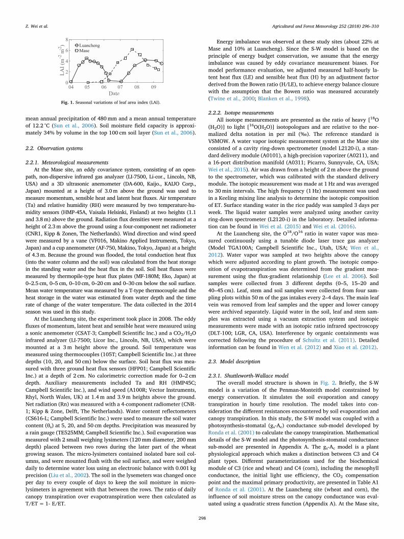
During the growing season in 2014, field observations were con-ducted at a rectangular experimental rice paddy field in Mase, Tsukuba,Japan (36° 03′ N, 140° 01′ E, elevation 12m above the mean sea level).Around the site, a field of about 150 ha was used exclusively forplanting rice (Oryza sativa L; Wei et al., 2016). The mean annual pre-cipitation and air temperature were approximately 1200mm and13.7 °C, respectively. Irrigation started on 24 April, 2014. Rice wassown on 2 May and was harvested at the end of August. The soil textureof the paddy fields is clay loam. During the full growing season, thefield was flooded to a mean water depth of 3.0 cm. Periodic measure-ments of leaf area index (LAI) are plotted in Fig. 1.

The other experiment was conducted at the Luancheng Agro-Ecosystem Experimental Station (37° 53′ N, 114° 41′ E), located in theNorth China Plain, which is a major agricultural region in China (Wenet al., 2012; Xiao et al., 2012). A field study was conducted in a winterwheat and summer corn rotation. Wheat (Triticum aestivum L.) wasplanted in November of 2007 and harvested on June 18, 2008, with amaximum LAI of 4.5 (Fig. 1) and a maximum height of 0.75m. Corn(Zea mays L.) was planted at the beginning of June before wheat har-vest and was harvested in mid-September. The corn canopy reached amaximum LAI of 4.2 and a maximum height of 2.77m on August 16(Fig. 1). The site is controlled by a semi-arid monsoonal climate, with a

Z. Wei et al. Agricultural and Forest Meteorology 252 (2018) 296–310

297

mean annual precipitation of 480mm and a mean annual temperatureof 12.2 °C (Sun et al., 2006). Soil moisture field capacity is approxi-mately 34% by volume in the top 100 cm soil layer (Sun et al., 2006).

2.2. Observation systems

2.2.1. Meteorological measurementsAt the Mase site, an eddy covariance system, consisting of an open-

path, non-dispersive infrared gas analyzer (LI-7500, Li-cor., Lincoln, NB,USA) and a 3D ultrasonic anemometer (DA-600, Kaijo., KAIJO Corp.,Japan) mounted at a height of 3.0m above the ground was used tomeasure momentum, sensible heat and latent heat fluxes. Air temperature(Ta) and relative humidity (RH) were measured by two temperature-hu-midity sensors (HMP-45A, Vaisala Helsinki, Finland) at two heights (1.1and 3.8m) above the ground. Radiation flux densities were measured at aheight of 2.3m above the ground using a four-component net radiometer(CNR1, Kipp & Zonen, The Netherlands). Wind direction and wind speedwere measured by a vane (VF016, Makino Applied Instruments, Tokyo,Japan) and a cup anemometer (AF-750, Makino, Tokyo, Japan) at a heightof 4.3m. Because the ground was flooded, the total conduction heat flux(into the water column and the soil) was calculated from the heat storagein the standing water and the heat flux in the soil. Soil heat fluxes weremeasured by thermopile-type heat flux plates (MF-180M; Eko, Japan) at0–2.5 cm, 0–5 cm, 0–10 cm, 0–20 cm and 0–30 cm below the soil surface.Mean water temperature was measured by a T-type thermocouple and theheat storage in the water was estimated from water depth and the timerate of change of the water temperature. The data collected in the 2014season was used in this study.

At the Luancheng site, the experiment took place in 2008. The eddyfluxes of momentum, latent heat and sensible heat were measured usinga sonic anemometer (CSAT-3; Campbell Scientific Inc.) and a CO2/H2Oinfrared analyzer (LI-7500; Licor Inc., Lincoln, NB, USA), which weremounted at a 3m height above the ground. Soil temperature wasmeasured using thermocouples (105T; Campbell Scientific Inc.) at threedepths (10, 20, and 50 cm) below the surface. Soil heat flux was mea-sured with three ground heat flux sensors (HFP01; Campbell ScientificInc.) at a depth of 2 cm. No calorimetric correction made for 0–2 cmdepth. Auxiliary measurements included Ta and RH (HMP45C;Campbell Scientific Inc.), and wind speed (A100R; Vector Instruments,Rhyl, North Wales, UK) at 1.4m and 3.9m heights above the ground.Net radiation (Rn) was measured with a 4-component radiometer (CNR-1; Kipp & Zone, Delft, The Netherlands). Water content reflectometers(CS616-L; Campbell Scientific Inc.) were used to measure the soil watercontent (θs) at 5, 20, and 50 cm depths. Precipitation was measured bya rain gauge (TE525MM; Campbell Scientific Inc.). Soil evaporation wasmeasured with 2 small weighing lysimeters (120mm diameter, 200mmdepth) placed between two rows during the later part of the wheatgrowing season. The micro-lysimeters contained isolated bare soil col-umns, and were mounted flush with the soil surface, and were weigheddaily to determine water loss using an electronic balance with 0.001 kgprecision (Liu et al., 2002). The soil in the lysemeters was changed onceper day to every couple of days to keep the soil moisture in micro-lysimeters in agreement with that between the rows. The ratio of dailycanopy transpiration over evapotranspiration were then calculated asT/ET=1- E/ET.

Energy imbalance was observed at these study sites (about 22% atMase and 10% at Luancheng). Since the S-W model is based on theprinciple of energy budget conservation, we assume that the energyimbalance was caused by eddy covariance measurement biases. Formodel performance evaluation, we adjusted measured half-hourly la-tent heat flux (LE) and sensible heat flux (H) by an adjustment factorderived from the Bowen ratio (H/LE), to achieve energy balance closurewith the assumption that the Bowen ratio was measured accurately(Twine et al., 2000; Blanken et al., 1998).

2.2.2. Isotope measurementsAll isotope measurements are presented as the ratio of heavy [18O

(H2O)] to light [16O(H2O)] isotopologues and are relative to the nor-malized delta notation in per mil (‰). The reference standard isVSMOW. A water vapor isotopic measurement system at the Mase siteconsisted of a cavity ring-down spectrometer (model L2120-i), a stan-dard delivery module (A0101), a high-precision vaporizer (A0211), anda 16-port distribution manifold (A0311; Picarro, Sunnyvale, CA, USA;Wei et al., 2015). Air was drawn from a height of 2m above the groundto the spectrometer, which was calibrated with the standard deliverymodule. The isotopic measurement was made at 1 Hz and was averagedto 30min intervals. The high frequency (1 Hz) measurement was usedin a Keeling mixing line analysis to determine the isotopic compositionof ET. Surface standing water in the rice paddy was sampled 3 days perweek. The liquid water samples were analyzed using another cavityring-down spectrometer (L2120-i) in the laboratory. Detailed informa-tion can be found in Wei et al. (2015) and Wei et al. (2016).

At the Luancheng site, the O18/O16 ratio in water vapor was mea-sured continuously using a tunable diode laser trace gas analyzer(Model TGA100A; Campbell Scientific Inc., Utah, USA; Wen et al.,2012). Water vapor was sampled at two heights above the canopywhich were adjusted according to plant growth. The isotopic compo-sition of evapotranspiration was determined from the gradient mea-surement using the flux-gradient relationship (Lee et al. 2006). Soilsamples were collected from 3 different depths (0–5, 15–20 and40–45 cm). Leaf, stem and soil samples were collected from four sam-pling plots within 50m of the gas intakes every 2–4 days. The main leafvein was removed from leaf samples and the upper and lower canopywere archived separately. Liquid water in the soil, leaf and stem sam-ples was extracted using a vacuum extraction system and isotopicmeasurements were made with an isotopic ratio infrared spectroscopy(DLT-100; LGR, CA, USA). Interference by organic containments wascorrected following the procedure of Schultz et al. (2011). Detailedinformation can be found in Wen et al. (2012) and Xiao et al. (2012).

2.3. Model description

2.3.1. Shuttleworth-Wallace modelThe overall model structure is shown in Fig. 2. Briefly, the S-W

model is a variation of the Penman-Monteith model constrained byenergy conservation. It simulates the soil evaporation and canopytranspiration in hourly time resolution. The model takes into con-sideration the different resistances encountered by soil evaporation andcanopy transpiration. In this study, the S-W model was coupled with aphotosynthesis-stomatal (gs-Ac) conductance sub-model developed byRonda et al. (2001) to calculate the canopy transpiration. Mathematicaldetails of the S-W model and the photosynthesis-stomatal conductancesub-model are presented in Appendix A. The gs-Ac model is a plantphysiological approach which makes a distinction between C3 and C4plant types. Different parameterizations used for the biochemicalmodule of C3 (rice and wheat) and C4 (corn), including the mesophyllconductance, the initial light use efficiency, the CO2 compensationpoint and the maximal primary productivity, are presented in Table A1of Ronda et al. (2001). At the Luancheng site (wheat and corn), theinfluence of soil moisture stress on the canopy conductance was eval-uated using a quadratic stress function (Appendix A). At the Mase site,

Fig. 1. Seasonal variations of leaf area index (LAI).

Z. Wei et al. Agricultural and Forest Meteorology 252 (2018) 296–310

298

because there was no soil moisture stress, the quadratic stress functionvalue was assigned a value of one.

The input data of the S-W model included air temperature, relativehumidity, net radiation, wind speed, atmospheric CO2 concentration,air pressure, soil temperature and moisture, LAI, and canopy height.The tunable parameter in the stomatal parameterization, the vaporpressure deficit constant D0 in Eq. (11) of Ronda et al. (2001), wasdetermined by minimizing the root mean square error (RMSE) betweenthe simulated and the observed latent heat flux. The optimization re-sults were D0=0.245 kPa for rice, D0= 0.250 kPa for wheat andD0=0.160 kPa for corn, respectively (Supplementary Table S1). It isnoted that our stomatal parameterization is different from that in thebig-leaf model proposed by Xiao et al. (2010) and applied to the sameexperiment at Luancheng (Xiao et al. 2012). The study by Xiao et al.(2012) aims to investigate temporal variability of foliage isotopecompositions. The version used by Xiao et al. contains two tunableparameters: D0 and the CO2 concentration constant a1, whereD0=0.50 kPa and a1=11.9 for wheat and D0=0.74 kPa anda1=4.2 for corn were determined by a nonlinear least squares methodto minimize the difference between the observed and the simulatedlatent heat flux. The present study adopted the original a1 parametervalues in Ronda et al. (2001) (a1= 9.1 for C3 and 6.6 for C4 plants).The canopy temperature (Tc) used by the gs-Ac sub-model (Fig. 2) wassolved iteratively until a stable value was reached.

Soil surface resistance (rss) is calculated as a function of soilmoisture content (Sellers et al., 1992; Appendix B).

Validation was performed against the eddy covariance ET mea-surements. The model calibration ensures that ET is unbiased but itdoes not guarantee that the total water vapor flux is partitioned prop-erly. The ET partition may be sensitive to how the net radiation is di-vided between the canopy and the substrate (Eq. A11) and to the soilsurface resistance parameterization (Eq. A18). A Monte Carlo analysiswas performed to quantify this error propagation. In this analysis, atotal of 1000 ensemble members were calculated, with errors in thelight extinction coefficient (kr, Eq. A11) and the two coefficients in Eq.A18 following a normal distribution with standard deviations of 10% ofthe original value.

To investigate the relationship of T/ET with LAI, soil moisture andcanopy resistance, we also applied to the S-W model to 7 AmeriFluxcrop sites, bringing the total number of sites to 10 (SupplementaryTable S1). Of these, 7 were irrigated (Luancheng Wheat, Luancheng

Corn, Maze Rice, US-NE1 Soybean, US-NE1 Corn, US-NE2 Soybean andUS-NE2 Corn) and 3 were rain-fed (US-NE3 Soybean, US-NE3 Corn andUS-RO3). Except for the vapor pressure deficit constant D0(Supplementary Table S1), all other parameters in the model wereunchanged. We chose these AmeriFlux sites because the soil moistureand LAI data were available at sufficient time resolutions to drive themodel simulation.

2.3.2. Isotopic partitioning approachThe isotope partitioning approach is based on mass balance con-

sideration for both the major and the minor isotopologues. Utilizing atwo end-member (E and T) mixing model, the partitioning can be ex-pressed as

= −−

T ET δ δδ δ

/ ET E

T E (1)

(Yakir and Sternberg, 2000). This equation requires that the isotopicratio of the ET, E and T fluxes be known from direct measurement ormodel estimation. In this study, δET at the Mase site was determinedfrom the vapor isotope measurement using the Keeling plot approach,and δET at the Luancheng site was measured with the flux-gradientmethod.

The isotopic composition of substrate evaporation (δE) was calcu-lated with the Craig and Gordon (hereafter C-G) model (Craig andGordon, 1965; Appendix C). Input variables of the C-G model includedthe isotopic ratios of vapor (δv) measured at the reference height abovethe canopy and soil (in the case of Luancheng) or surface (in the case ofMase) water (δs), air temperatures, soil or surface water temperature,relative humidity, and the kinetic fractionation associated with sub-strate evaporation (εk). Different εk values were applied to the two sitesto account for the fact that substrate evaporation originated from twodifferent media (soil in Luangcheng and standing water in Mase; Ap-pendix C): A constant εk value of 21‰ based on the chamber eva-poration study of Kim and Lee (2011) was used for Mase and theparameterization of Wen et al. (2012) was used for Luancheng.

The isotopic composition of transpiration (δT) was estimated undertwo different assumptions. Under the steady-state assumption (SSA), δTwas assumed to be the same as the delta value of stem water. Under thecondition of non-steady state (NSS) isotopic behavior of transpiration,δT is also affected by temporal changes in foliage water content (W) andthe transpiration rate (T). To determine δT in non-steady state, themodel proposed by Farquhar and Cernusak (2005), accounting for thechange in the water content and the Péclet effect, was used. The mea-sured W and the isotopic ratio of stem water are required by this modelas input variables. At the Luancheng site, a seasonal time series of Wwas established by linear interpolation between weekly W measure-ments. Superimposed on the seasonal variation was a diurnal variationaccording to the diurnal composite W measured during intensivecampaigns (Xiao et al., 2010; Xiao et al., 2012). The seasonal mean Wwas 159.7 gm−2 for wheat and 154.1 gm−2 for corn. The other inputvariables needed by the NSS model, the transpiration rate, canopytemperature, relative humidity in reference to canopy temperature(RHc), and the resistance terms were determined by the S-W modeloutputs (Appendix A). The resistance terms were used to determine thekinetic factor for T (Lee et al. 2009).

At the Mase site, because of the lack of stem water isotope mea-surement, we assumed that the δ value of stem water was the same asthat of the surface water. A typical value of W of 110 gm−2 for riceplant (Ishihara et al., 1974) was assumed for the rice growing season.Time changes in W were not considered; Xiao et al. (2012) showed thatthe foliage isotope enrichment is not sensitive to time variations in W.

In addition to δE and δT the transpiration isotopic submodel alsocalculates the isotopic composition of bulk leaf water δL,b. Although notused for ET partitioning, δL,b is a useful variable to understand the non-steady state isotopic behaviors and to gage the submodel performance.To evaluate the transpiration isotopic submodel, we compared the

Fig. 2. Schematic representation of the two source-model and its relationship to theisotopic tracer method. S-W: Shuttleworth and Wallace model; SSA: steady state isotopicbehavior of transpiration; NSS: non-steady state isotopic behavior; C-G: Craig-Gordonmodel: Ag-gc,w: canopy resistance model developed by Ronda et al. (2001).

Z. Wei et al. Agricultural and Forest Meteorology 252 (2018) 296–310

299

modeled δL,b against the measured values. Detailed information aboutthe δT and δL,b equations can be found in Appendix C.

In this study, we quantify T/ET using three methods, the S-W model,a combination of eddy covariance and lysimeter measurements (forwheat only), and an isotopic partitioning approach based on the SSAand NSS δT estimation. Fig. 2 shows the relationships between the firstand the third methods.

2.4. Performance evaluation and sensitivity analysis

Four performance measures, including root mean squares error(RMSE), index of agreement (I), bias index (BI), and coefficient ofvariation (R2), were used to evaluate the model performance, as

∑= ⎡

⎣⎢ − ⎤

⎦⎥

=

RMSEN

S M1 ( )i

N

i i1

21/2

(2)

= −∑ −

∑ − + −=

=

IS M

S M M M1

( )

(| | | |)iN

i i

iN

i i

12

12 (3)

∑= −=

BIN

M S1 ( )i

N

i i1 (4)

=⎡

⎣

⎢⎢

∑ − −

∑ − ∑ −

⎤

⎦

⎥⎥

=

= =

RS S M M

M M M M

( )( )

( ) ( )iN

i i

iN

i iN

i

2 1

12

12

2

(5)

where N is total number of observations, Si is modeled value, and Mi isobserved value.

A sensitivity analysis was conducted to quantify model errors thatmay arise due to uncertainties in the measured input variables. Theapproach was proposed by Beven (1979) and Wang and Yamanaka(2014). The sensitivity coefficient (SCj) is given by

∑=∂∂=

SCN

OP

PO

1j

i

Ni j

i j

i j

i j1

,

,

,

, (6)

where Pj is the jth variable in question, subscript i denote the ith ob-servation, N is total number of observations, O is output variable, whichis either the ET flux or the flux ratio T/ET. The differential ∂ ∂O P/i j i j, , isestimated as:

∂∂

=−−

OP

O OP P**

i j

i j

P P,

, (7)

where OP* is the predicted O with a provisionally-assumed value of P,

and OP is the predicted O with the default model variable value or themeasured input variable value (Beven, 1979). A positive SCj value of0.1 means that a 1% increase in Pj induces a 0.1% increase in O. Notethat only daytime (07:00–17:00 local time) data were used for thissensitivity analysis because nighttime water vapor flux is a minorcomponent of the daily mean flux to the atmosphere.

3. Results

3.1. Performance of the S-W model at different time scales and differentsites

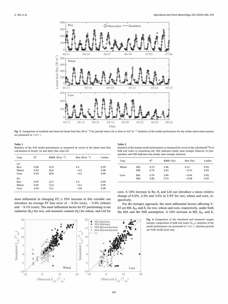
In general, the model has successfully simulated ET for the threeecosystems. No obvious bias is detected during the whole growingseasons. As an example, Fig. 3 shows variations of the simulated andmeasured hourly latent heat flux during the peak growing season (LAIclose to 4) for rice, wheat and corn. The model performance statisticsbased on hourly values for the whole season are shown in Table 1a. Themodel slightly underestimates ET for rice and wheat, by 2% and 1%,respectively, and slightly overestimates ET for corn by about 1%. Thedaily ET means have smaller RMSEs than the hourly means (Table 1b).

The seasonal mean bias errors of the whole-ecosystem latent heat fluxare 4.3Wm−2,−0.4Wm−2 and−0.8Wm−2 for rice, wheat and corn,respectively.

The model was further tested using the data measured at AmeriFluxsites US-NE1, US-NE2, US-NE3 and US-RO3 consisting of corn-soybeanrotation. The tunable parameter (D0) in the stomatal parameterizationwas set to 0.35 and 0.40 for soybean and corn ecosystems, respectively(Supplementary Table S1). The S-W model reproduced the observed ETvery well, with a bias within 10% and a high correlation (R2 > 0.87;Supplementary Figs. S1 and S2).

3.2. Isotopic composition of canopy foliage water

A comparison of the observed and modeled isotope composition ofthe bulk leaf water (δL,b) is given in Fig. 4. A summary of statistics isshown in Table 2. The isotope composition of the leaf water is simu-lated reasonably well, with R2 equal to 0.73, I index of 0.92, BI of0.13‰ and RMSE of 2.46‰ using SSA for wheat, and R2 equal to 0.76(0.82), I index of 0.92 (0.93), BI of 0.04‰ and RMSE of 2.89‰ usingSSA for corn; using NSS, the R2 is equal to 0.74, I index is 0.92, BI is−0.31‰ and RMSE is 2.63‰ for wheat, and R2 is equal to 0.82, I indexis 0.93, BI is −0.58‰ and RMSE is 2.74‰ for corn.

Similar to Xiao et al. (2012), the SSA and the NSS model producednearly identical results for the daytime (9:00–16:00 local time) and themain discrepancy occurred in the nighttime (Fig. 4). The low sensitivityof the simulated δL,b to the SSA in the daytime is related to the shortturnover time of foliage water (less than 1 h, Wang et al., 2015) andlack of the Péclet effect at the canopy scale (Xiao et al., 2010). Thelarger nighttime differences between the NSS and the SSA results can bepartially explained by a large foliage water turnover time (greater than200 h; Wang et al., 2015) at night. Because isotopic composition in thebulk leaf plays a major role in the isotopic exchange between the eco-system and atmosphere, the good correlation between the simulatedand observed isotopic composition in the canopy foliage suggests thatour model is reasonably robust.

3.3. T/ET seasonal variations

Fig. 5 shows the seasonal variations of T/ET based on the S-W modeland on the isotope approach deploying the SSA and the NSS assumption.Here, the T/ET variation displays a strong seasonal cycle, varying between0.0–0.6 for the SW model and 0.2–1.0 for the isotope method for rice,0.5–1.0 for the measurement, 0.6–0.9 for the SW model and 0.8–1.0 forthe isotope method for wheat, and 0.2–0.7 for the SW model and 0.2–1.0for the isotope methods for corn. According to the S-W model, T/ET forrice and corn increase almost continuously with the vegetation growth inthe early growing season, and becomes relatively constant after the cropsestablished dense foliage (LAI > 2.5). Similar trend can be found in theisotope results, although a higher T/ET ratio can be found in most of theobservation days. The difference in the daily T/ET between the isotopemethod and the S-W numerical modeling ranges from 0 to 0.5 for rice, 0 to0.2 for wheat and 0 to 0.4 for corn. For seasonal timescale estimation, T/ET is not sensitive to the SSA assumption (Fig. 5), although many studieshave documented the impact of NSS on diurnal δT estimations (Lai et al.,2006; Dubbert et al., 2013; Dubbert et al., 2014b). For the whole mea-surement period, the S-W model results show that T/ET is 0.50, 0.84 and0.64, and the isotopic approach shows that T/ET is 0.74, 0.93 and 0.81, forrice, wheat and corn, respectively (Table 3). The two-source model resultsare in better agreement than the isotopic method with the soil lysimeterand eddy covariance measurement made during the same time period forwheat (T/ET=0.87).

3.4. Sensitivity analysis

Supplementary Table S2 summarizes the sensitivity of ET and T/ETto the measured input variables. In the case of the S-W model, RH is the

Z. Wei et al. Agricultural and Forest Meteorology 252 (2018) 296–310

300

most influential in changing ET; a 10% increase in this variable canintroduce an average ET bias error of −9.2% (rice), −5.9% (wheat)and −9.1% (corn). The most influential factor for ET partitioning is netradiation (Rn) for rice, soil moisture content (θs) for wheat, and LAI for

corn. A 10% increase in Rn, θs and LAI can introduce a mean relativechange of 6.0%, 2.3% and 3.6% in T/ET for rice, wheat and corn, re-spectively.

For the isotopes approach, the most influential factors affecting T/ET are RH, δET and δv for rice, wheat and corn, respectively, under boththe SSA and the NSS assumption. A 10% increase in RH, δET and δv

Fig. 3. Comparison of modeled and observed latent heat flux (Wm−2) for periods when LAI is close to 4m2m−2. Statistics of the model performance for the whole observation seasonsare presented in Table 1.

Table 1Statistics of the S-W model performance as measured by errors in the latent heat fluxcalculations at hourly (a) and daily time steps (b).

Crop R2 RMSE (Wm−2) Bias (Wm−2) I-index

(a)Rice 0.96 33.9 4.3 0.99Wheat 0.93 42.6 −0.3 0.98Corn 0.94 28.8 −0.5 0.99

(b)Rice 0.97 12.7 4.3 0.99Wheat 0.95 14.5 −0.4 0.99Corn 0.94 12.1 −0.8 0.98

Fig. 4. Comparison of the simulated and measured oxygenisotopic composition of bulk leaf water (δL,b). Statistics of themodel performance are presented in Table 2. Daytime periodsare 9:00–16:00 local time.

Table 2Statistics of the isotope model performance as measured by errors in the calculatedδ18O ofbulk leaf water in Luancheng site. SSA indicates steady state isotopic behavior of tran-spiration and NSS indicates non-steady state isotopic behavior.

Crop R2 RMSE (‰) Bias (‰) I-index

Wheat SSA 0.73 2.46 0.13 0.92NSS 0.74 2.63 −0.31 0.92

Corn SSA 0.76 2.89 −0.04 0.92NSS 0.82 2.74 −0.58 0.93

Z. Wei et al. Agricultural and Forest Meteorology 252 (2018) 296–310

301

produces a relative change in T/ET by −4.8% (rice), −2.1% (wheat)and −2.5% (corn). Consequently, the estimated values of T/ET seemrobust, as long as errors in the measured variables are bounded to 10%of the reported values. We do not expect the measurement errors in RH,δv and other micrometeorological variables to exceed this threshold.However, as explained in Section 4.3, errors in δET can be larger thanthis.

4. Discussion

4.1. Comparison with previous studies

Several isotope-enabled land-surface models have been developedto simulate ecosystem processes related to the hydrologic cycle. Xiaoet al. (2010) developed a big leaf model to simulate ET and isotopicwater pools and fluxes, showing good performance (RMSE of 57Wm−2

for latent heat flux and 2.9‰ for δL,b) for a soybean ecosystem. Theirsimulation was restricted to the period when the canopy was fullyclosed (LAI > 2), due to the neglect of soil evaporation in their model.Our model treats T and E and their isotope compositions separately.Under conditions of low LAI (< 2), the RMSE of our model is28.8Wm−2 for latent heat flux and 1.97‰ (2.92‰) for NSS (SSA) for

δL,b for the corn experiment; these errors are comparable to those underhigh LAI (> 2) conditions: the RMSE is 28.0Wm−2 for the latent heatflux and 2.34‰ (2.40‰) for NSS (SSA) δL,b. The consistent resultssuggest that our model is suitable for simulating the seasonal watervapor fluxes and their isotopic variations.

Wang et al. (2015) have developed a two-source model called Iso-SPAC for partitioning evapotranspiration, with RMSEs of 37.2Wm−2

and 1.69‰ for the latent heat flux and δL,b, respectively, for a grasslandecosystem. Iso-SPAC is based on a bulk transfer method and treats theenergy balance of both vegetative canopy and at the ground. TheNewton–Raphson (NR) iteration scheme is used to solve the canopytemperature and the subtract temperature (Wang et al., 2015). A fur-ther application of this model was conducted in an arid artificial oasiscropland ecosystem with high-frequency water vapor isotope mea-surements (Wang et al., 2016). However, the uncertainties becomelarger there, with RMSEs of 45.9Wm−2 for the latent heat flux and4.65‰ for δL,b, suggesting that some of the model parameters needfurther tuning to improve the model’s generality. The National Centrefor Atmospheric Research (NCAR) stable isotope-enabled Land SurfaceModel (ISOLSM) has also be used to simulate ET and its isotopic com-ponents (Riley et al., 2003; Cai et al., 2015). In Cai et al. (2015), theISOLSM model is restricted mostly to a dry period between January 16and 25, 2011, with an RMSE of 58.1W m-2 for the latent heat flux. (TheRMSE increases to 88.9Wm−2 for a wet period for a mixed naturaleucalyptus forest.). In our study, the RMSE of the latent heat flux is42.6Wm−2 for the wheat season and 28.8Wm−2 for the rice season(Table 1). The ISOLSM uses a two-leaf (sunlit and shaded) formulationfor canopy processes. Our results indicate that the simpler one-leafformulation actually works better, at least for the simulation of watervapor flux.

The T/ET ratio based on the S-W model compares favorably withthose reported in the literature for cropland ecosystems. Our estimatedfull growing season T/ET for rice (0.50) is lower than for flooded wheat(0.67–0.75) reported by Balwinder-Singh et al. (2011) on the basis ofmicrolysimeter measurements in Punjab, India. By coupling a land-surface and a crop growth model, Maruyama and Kuwagata (2010)showed that T/ET is 0.45 during a rice growth period in Tsukuba,Japan. According to weighting lysimeter and micro-lysimeter mea-surements made by Zhang et al. (2013), transpiration fraction duringthe full crop season is generally between 0.64 and 0.95 for a full wheatseason consisting of mature and immature periods, and between 0.65and 0.94 for a summer maize, with a whole season means of 0.72 and0.60, respectively, for a winter-wheat and summer maize rotationcropland in North China Plain. Xu et al. (2016) partitioned ET via atwo-source variational data assimilation system, showing a dominantcontribution from T to the total ET (T/ET > 0.8) for a summer cornfield. Soil lysimeter and whole-canopy lysimeter measurements pub-lished by Liu et al. (2002) indicate that canopy transpiration comprises0.79 and 0.70 of the total evapotranspiration for a mature wheat andsummer corn system, respectively, in the Luancheng site; for compar-ison, the T/ET ratio in our study is 0.84 for mature wheat growth phaseand 0.64 for the full season of the corn growth phase.

Our isotope-based T/ET, which shows that T/ET is 0.74, 0.93 and0.81 during the measurement period for rice, wheat and corn, respec-tively, is generally consistent with other isotopic studies. Wang andYakir (2000) reported a value of 0.96 to 0.98 for a mature wheat fieldwith a dense canopy. Wen et al. (2016) found that the relative con-tribution of daily T to ET ranges from 0.71 to 0.96 with a mean of0.87 ± 0.05 for the growing season of a corn crop. Zhang et al. (2011)showed T varies from 60% to 83% of the total ET during a winter wheatseason in North China Plain.

4.2. Factors controlling T/ET

Our S-W model results confirm that T/ET is controlled by LAI at theseasonal timescale (Hu et al., 2009; Good et al., 2014; Wang and

Fig. 5. Seasonal variations of T/ET determined by the isotope-based method (both SSAand NSS) for midday periods (11:00–15:00) and the daily T/ET determined by the S-Wtwo-source model and the lysimeter / eddy covariance method.

Table 3Comparison of ET-weighted T/ET for the whole observation periods using three differentmethods.

Crop S-W model Isotope Lysimeter / eddy covariance measurement

SSA NSS

Rice 0.50 0.77 0.74 –Wheat 0.84 0.93 0.93 0.87Corn 0.64 0.82 0.81 –

Z. Wei et al. Agricultural and Forest Meteorology 252 (2018) 296–310

302

Yamanaka, 2014; Wei et al., 2015; Berkelhammer et al., 2016). Theday-to-day variations of T/ET for rice and corn are primarily controlledby LAI through its regulation of canopy radiation interception and ca-nopy resistance; this relationship can be described with power functions(Fig. 6). For low LAI conditions (LAI≤ 2.5), the T/ET ratio increasesrapidly with increasing LAI. At higher LAI values (LAI > 2.5), eventhough LAI increases rapidly with time (Fig. 1), the ratio become lesssensitive to LAI increase (Figs. 5 and 6). The standard deviation of T/ETfor LAI≤ 2.5 is 0.17, 0.18 for rice and corn, while for 2.5 < LAI < 6, itdecreases to 0.07, 0.04, 0.03 for rice, wheat and corn, respectively. Thissuggests processes controlling T and E may be coupled in ways tomaintain a stable T/ET ratio. The low LAI sensitivity under high LAIconditions is confirmed by soil lysimeter and eddy covariance mea-surements in the wheat ecosystem (Fig. 6). Some of the day-to-dayvariations in T/ET may have been influenced by weather fluctuations(Fig. 5), but the strong correlation between T/ET and LAI (R2 of 0.86 forrice and 0.94 for corn) implies that the role of weather is minor incomparison to that of vegetation density. It is noted that the values ofT/ET for wheat reported in Fig. 6 start at LAI > 2.4 due to lack ofobservations before that.

A recent meta-analysis reveals that among the 6 major global ve-getation types, the T/ET versus LAI relationship of agricultural cropsshows the largest spread (Wei et al., 2017). In an effort to understandthe underlying causes of the spread, here we compare the monthly T/ETpredicted by the S-W model with the regression result based on theglobal crop synthesis dataset of Wei et al. (2017) (Fig. 7). The T/ETvalues for corn and rice are lower than the global mean, and those forwheat and the Ameriflux sites follow closely the global trend line. Allthe data are within the 95% confidence bound of the global regressionresult.

Soil moisture may exert some influence on T/ET. In the case of rice,there was no soil moisture stress, meaning that soil moisture contentwas set to 100% of the field capacity. In the case of wheat, which hasthe same photosynthetic mode (C3) as rice, daily soil moisture variedbetween 0.20 and 0.34 (volume fraction), with an average of 0.27during the growing season. The daily soil moisture for corn varied be-tween 0.26 and 0.38 with an average of 0.31. The opposite order be-tween T/ET (wheat > corn > rice) and soil moisture (wheat <corn < rice) under the same LAI condition indicates increasing soilmoisture may reduce T/ET via increasing soil E. Other authors havealso emphasized the role of soil water content in controlling T/ET (Huet al. 2009; Liu et al., 2002). The water used for plant transpirationcomes from the whole root zone, while the soil evaporation is con-trolled by top-soil moisture. Taking the example of wheat, the maindepths of root water uptake are from 0 to 40 cm depths, while soilevaporation is controlled by soil moisture at the depth less than 20 cm(Zhang et al., 2011). Under dry conditions, although the moisture in the

Fig. 6. Relationships between T/ET and LAI. Lines represent best fit regressions in-dicated.

Fig. 7. Monthly T/ET predicted by the S-W model as a function LAI. The solid line re-presents the trend of a global crop data with the 95% confidence bound indicated by thedashed lines. Error bars are± 1 standard deviation of Monte Carlo ensemble members.

Z. Wei et al. Agricultural and Forest Meteorology 252 (2018) 296–310

303

root zone can meet the requirement for transpiration, soil evaporationmay encounter a large surface resistance in the top soil layer, thushaving the tendency to reduce E and increase T/ET. This is generallyconsistent with the concept proposed by Maxwell and Condon (2016),who suggests subsurface water plays a substantial role in the parti-tioning of evapotranspiration, and is also in agreement with the modelsensitivity of wheat T/ET to soil moisture (Supplementary Table S2).

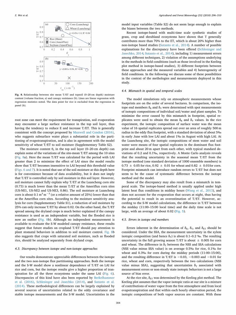
The moisture content θs in the top soil layer (0–20 cm depth) canexplain some of the variations of the site-mean T/ET among the 10 sites(Fig. 8a). Here the mean T/ET was calculated for the period with LAIgreater than 2 to minimize the effect of LAI since the model resultsshow that T/ET becomes insensitive to LAI beyond this threshold value(Figs. 6 and 7). It is noted that use of the soil moisture at this depth hereis for convenience because of data availability, but it does not implythat T/ET is controlled only by soil moisture in this soil layer. However,soil moisture cannot fully explain why T/ET at the Luancheng corn site(0.73) is much lower than the mean T/ET at the Ameriflux corn sites(US-NE1, US-NE2 and US-NE3, 0.86). The soil moisture at Luanchengcorn is about 0.1 m3m−3 (or a relative amount of 25%) lower than thatat the Ameriflux corn sites. According to the moisture sensitivity ana-lysis for corn (Supplementary Table S1), a reduction of soil moisture by25% can only increase T/ET by about 0.02. On the other hand, the T/ETspread among the dryland crops is much better explained if the canopyresistance is used as an independent variable, but the flooded rice isnow an outlier (Fig. 8b). Although no independent measurement isavailable to evaluate the S-W modeled canopy resistance, these resultssuggest that future studies on cropland T/ET should pay attention toplant stomatal behaviors in addition to soil moisture control. Fig. 8balso suggests that crops with saturated soil moisture, such as floodedrice, should be analyzed separately from dryland crops.

4.3. Discrepancy between isotope and non-isotope approaches

Our results demonstrate appreciable differences between the isotopeand the two non-isotope flux partitioning approaches. Both the isotopeand the S-W model show a nonlinear dependence of T/ET on LAI forrice and corn, but the isotope results give a higher proportion of tran-spiration for all the three ecosystems under the same LAI (Fig. 6).Discrepancies of this kind have also been reported by Berkelhammeret al. (2016), Schlesinger and Jasechko (2014), and Sutanto et al.(2014). These methodological differences can be largely explained byseveral sources of uncertainties related to the eddy covariance andstable isotope measurements and the S-W model. Uncertainties in the

model input variables (Table S2) do not seem large enough to explainthe biases between the two methods.

Recent isotope-based with multi-time scale synthetic studies ofgrass, crop and shrubland ecosystems have shown that T generallycontributes more than 70% to the ET, which is about 20% higher thannon-isotope based studies (Sutanto et al., 2014). A number of possibleexplanations for the discrepancy have been offered (Schlesinger andJasechko, 2014; Sutanto et al., 2014), including 1) measurement errorsamong different techniques, 2) violation of the assumptions underlyingin the methods in field conditions (such as those involved in the Keelingplot method in isotope-based studies), 3) different footprints betweenthese approaches and the measured variables and 4) heterogeneity offield conditions. In the following we discuss some of these possibilitiesin the context of the methologies and measurements deployed in thisstudy.

4.4. Mismatch in spatial and temporal scales

The model simulations rely on atmospheric measurements whosefootprints are on the order of several hectares. In comparison, the iso-tope end members δE and δT were determined with spot measurementsof isotopic compositions of individual soil/water and plant samples. Tominimize the error caused by this mismatch in footprint, spatial re-plicates were used to obtain the mean δE and δT values. In the riceexperiment, the isotopic composition of surface water was the meanvalue of 16 spatial replicates spread out over an area of roughly 500mradius in the eddy flux footprint, with a standard deviation of about 5‰in early June with low LAI and about 1‰ in August with high LAI. Atthe Luancheng site, the isotopic compositions of stem water and soilwater were means of four spatial replicates in the dominant flux foot-print and about 20m apart from each other, with typical standard de-viations of 0.2 and 0.1‰, respectively. A Monte Carlo analysis revealsthat the resulting uncertainty in the seasonal mean T/ET from theisotope method (one standard deviation of 1000 ensemble members) is0.73 ± 0.05 for rice, 0.92 ± 0.01 for wheat and 0.82 ± 0.01for corn.Footprint mismatch can introduce random errors to T/ET but does notseem to be the cause of systematic difference between the isotopemethod and the model.

Some of the discrepancy may also result from a mismatch in tem-poral scale. The isotope-based method is usually applied under highlatent heat flux conditions in midday hours (Wang et al., 2013), anddoes not account for the evaporation that occurs at night, thus havingthe potential to result in an overestimation of T/ET. However, ac-cording to the S-W model calculations, the difference in T/ET betweenthe midday (11:00–15:00 local time) and the daily time scale is notlarge, with an average of about 0.02 (Fig. 5).

4.5. Errors in isotope end members

Errors inherent in the determination of δE, δT, and δET should beconsidered. Under the SSA, the measurement uncertainty in the xylemisotopic composition (and hence δT) is about 0.1–0.2 ‰. The resultinguncertainty in the full growing season T/ET is about ± 0.005 for cornand wheat. The difference in δT between the NSS and SSA calculations(NSS value minus SSA value) is on average 0.5‰ for rice, 0.1‰ forwheat and 0.3‰ for corn during the midday periods (11:00–15:00),and the resulting difference in T/ET is −0.03, −0.003 and −0.01 forrice, wheat and corn, respectively between the two calculations (NSSvalue minus SSA), suggesting that uncertainties δT associated withmeasurement errors or non-steady state isotopic behaviors is not a largesource of bias error.

At the rice site, δET was determined by the Keeling plot method. TheKeeling plot assumes that the vapor isotopic ratio at our site is a mixtureof contributions of water vapor from the free atmosphere and from localevapotranspiration and that within each hourly observation period, theisotopic compositions of both vapor sources are constant. With these

Fig. 8. Relationship between site mean T/ET and topsoil (0–20 cm depth) moisturecontent (volume fraction; a) and canopy resistance (b). Lines are linear regression withregression statistics noted. The data point for rice is excluded from the regression inpanel (b).

Z. Wei et al. Agricultural and Forest Meteorology 252 (2018) 296–310

304

assumptions, the isotopic signature of evapotranspiration can be cal-culated as the y-intercept of a linear regression of the vapor delta valueversus the inverse of the water vapor mixing ratio (Keeling, 1958).Although the Keeling plot approach is robust when applied to hightemporal resolution data (Good et al., 2012), the assumptions under-lying this method may not have been met perfectly in field conditions(Wei et al., 2015). Using the 1-Hz vapor isotopic data obtained by Wenet al. (2016) for an irrigated corn crop in western China, we comparedthe δET derived from the Keeling plot approach with the δET measuredby the flux-gradient method. The flux-gradient method does not invokethe assumptions involved in the Keeling plot analysis, so it is likelymore accurate. We found that during the midday periods, the twomethods are highly correlated, but the Keeling method is biased low by2.2‰ when compared with the flux gradient method (SupplementaryFig. S3). Assuming the same bias for the Mase site, the growing seasonmean T/ET would decrease from 0.74 to 0.65, bringing the isotopeestimate to a closer agreement with the result produced by the S-Wmodel (0.50).

A laboratory test shows that the δET derived from the flux-gradientmeasurement using the type of analyzer deployed at Luancheng has arandom error of 0.30‰ (Wen et al., 2012) and a systematic low bias of0.33‰ (Lee et al., 2007). According to Huang and Wen (2014), therandom error increases significantly under field conditions, to anaverage of 4.6‰ for an oasis crop ecosystem, while Hu et al. (2014)found that the random error is about 7.9‰ for a temperate grasslandunder low evapotranspiration conditions. A random error of 4.6‰ inδET would result in a relative uncertainty of 43%, 31%, 32% for T/ETfor the rice paddy, wheat and corn, respectively. Such an error rangewould be a problem for understanding day-to-day fluctuations butshould not cause a systematic bias in the seasonal mean T/ET. Therelative bias error in T/ET arising from a low bias error of 0.3‰ in δETis less than 2%.

With regard to δE, potential errors can result from 1) kinetic frac-tionation parameterization (Dubbert et al., 2013), 2) temporal inter-polation of substrate δ (Rothfuss et al., 2013), and 3) evaporationwater source in the case of the dryland systems (Dubbert et al., 2013;Werner and Dubbert, 2016). Until now, there is still no agreement onthe estimation of the kinetic fractionation factor εk in the C-G model.At the Mase site, the εk value (21‰) comes from a chamber eva-poration experiment (Kim and Lee, 2011). The same experiment alsoreveals that the interfacial surface water undergoing evaporation isisotopically 7.5–8.9‰ more enriched than the bulk water below thesurface. If an 8.9‰ interfacial enrichment was assumed for the waterin the rice field, the T/ET for the full rice season would decrease from0.74 to 0.65 and would improve the comparison with the S-W model(T/ET= 0.50). Alternatively, if we assume that δET is biased low by2.2‰ and all other errors occur in εk, reducing the seasonal mean T/ETto 0.50 will require a value of 43‰ for εk associated with the eva-poration of the standing water in the paddy field, which exceeds themolecular limit of 32‰ and is therefore unacceptable. It appears thatat the high T/ET bias of the isotopic method at the Mase site is a resultof biases in δET and surficial enrichment of the paddy water below thecanopy.

In the case of wheat and corn, it is difficult to determine which soillayer δ should be used for the isotopic composition of soil water un-dergoing evaporation, and yet this variable is a critical C-G modelinput. Currently, δE was calculated with the soil water δ measured atthe 5 cm depth. Hu et al. (2014) showed that in a grass field, the dif-ference of midday δ between 5 cm and 15 cm depths is relatively small(2.8‰) on days with high soil water content, but become larger (7.7‰)on days with low soil moisture. At the Luancheng site, the verticalvariations in the soil water delta value are 1.75‰ on average amongthe 5 cm, 15 cm and 25 cm soil depths. A model simulation suggests thatthe depth with the most enriched isotopic signal is found at the soilevaporation front (Mathieu and Bariac,1996). A theoretical estimate ofδ at the soil evaporation front is about 1–6‰ more enriched as

compared to the values measured in the top 1 cm of the soil (Rothfusset al., 2013). Dubbert et al. (2013) also found a strong increase in δ atthe top of the soil profile with the most enriched δ values at the 0–5 cmsoil depth. It is possible that the δ value measured at the 5 cm depth wasan underestimate of the δ value of water at the soil evaporation front atthe Luancheng site. To match the seasonal mean T/ET ratio producedby the S-W model, a 7.9‰ and 13.0‰ enrichment of soil δ above the δvalue observed at the 5 cm depth is required for wheat and corn, re-spectively, under the SSA. Alternatively, this extra enrichment leads tothe hypothesis that evaporative enrichment is confined to a thin film ofwater surrounding soil particles whose isotopic composition is muchhigher than the measured value of the bulk soil water. In this regard,the process would be similar to that involved in evaporation in the plantleaf where the water undergoing evaporation is much more enrichedthan the bulk leaf water.

4.6. Errors in eddy covariance flux

The discrepancy between the isotope and the non-isotope approach(eddy covariance and lysimeter combination) cannot be fully ex-plained by the isotopic measurements errors. Based on the principle ofenergy budget conservation, the evapotranspiration measured by theeddy covariance instrument had a bias error of about 3%, 16% and22% for wheat, corn and rice, respectively, if we assumed the availableenergy and the Bowen ratio were accurately measured. This under-estimation introduced some uncertainty for ET partitioning using theeddy covariance –lysimeter combination. In this combination ap-proach, the T flux was computed as the difference between the ET fluxobserved with eddy covariance and E flux observed with the lysi-meters. If we used the observed ET before adjustment for energy bal-ance, the seasonal T/ET was 0.87 for wheat (Table 3). If we adjustedthe eddy-covariance ET by forcing energy balance closure, the sea-sonal T/ET of wheat would increase slightly to 0.88, which is closer tothat derived from isotope approach. The energy balance adjustmentwould have a larger effect for rice and corn had there been lysimetermeasurements during these crop seasons. This point can be demon-strated by a hypothetical analysis. If we assume that the modeled E isan accurate representation of evaporation, we can compute T as thedifference between the observed ET and the modeled E. The seasonalT/ET is 0.34, 0.83 and 0.59 for rice, wheat and corn, respectively,before energy balance adjustment, and increases to 0.49, 0.84 and0.64 for rice, wheat and corn, respectively, if the observed ET is ad-justed using the Bowen ratio method.

4.7. Errors in the S-W model

The S-W model was calibrated against the ET measured with eddycovariance and adjusted for energy balance, by tuning one parameter inthe canopy resistance parameterization (the vapor pressure deficitconstant D0). This tuning ensured that the total water vapor flux(Figs. 3, S2 and S3) and the canopy resistance were unbiased. No tuningwas made to three other parameters that may affect the ET partitioning,namely the light extinction coefficient used to divide the total net ra-diation into the canopy and the substrate components (Eq. A18) and thetwo empirical coefficients in the soil surface resistance parameteriza-tion (Eq. A11). The Monte Carlo analysis suggests that the error in T/ETassociated with uncertainties in these parameters is about 0.1 (onestandard deviation of 1000 ensemble members) for wheat and corn andis negligible for rice (Fig. 7). In other words, the isotopic T/ET forwheat is within the error range of the model, but those for corn and riceare not.

The model error for rice can be omitted because the surface re-sistance parameterization was avoided due to the saturation condition.The result supports the above conclusion, that the high T/ET bias of theisotopic method at the Mase site is most likely the result of biases in δETand surficial enrichment of the paddy water below the canopy.

Z. Wei et al. Agricultural and Forest Meteorology 252 (2018) 296–310

305

5. Conclusions

The two-source model presented in this study shows good agree-ments with observed isotope composition in the bulk leaf water andwith the ET flux. The agreement of transpiration fraction T/ET calcu-lated by the two-source model (0.83) for the wheat growing season andthe T/ET based on soil lysimeter and eddy covariance measurements(0.87), highlights the robustness of the two-source model for ET par-titioning. On the other hand, the transpiration fraction T/ET estimatedby the isotope method is higher than that obtained with the two-sourcemodel for all the three crops (rice, wheat and corn). A Monte Carloanalysis shows that the difference between the two methods is largerthan the model uncertainty for rice and corn. One potential cause of thehigher T/ET for rice via the isotopic method is that the interfacialsurface water undergoing evaporation under the canopy may have beenmuch more enriched than the measured delta value of the bulk water.

The model-estimated T/ET varies from 0 to 1, with a near con-tinuous increase over time in the early growing season when LAI wasless than 2.5 and then convergence towards a stable value beyond LAIof 2.5. The seasonal change in T/ET is well described by a function ofLAI, implying that LAI was a first-order factor affecting ET partitioning.The isotope-based results also reveal a dependence on LAI. The de-pendence of T/ET on LAI is a well-known relationship and is useful for

benchmarking the isotope method. The two-source model calculationsmade for 7 Ameriflux crop sites reveal that this relationship is sensitiveto site soil moisture availability and canopy resistance.

The current two-source model is an improvement over previoustwo-source models, most of which are based on the Jarvis-Stewartstomatal empirical parameters. Our model is parameterized accordingto plant physiological constraints and directly links the terrestrial waterflux with the carbon flux. The fact that only one parameter requirestuning makes our model more versatile than some other models. Themodel code is available at the open-source platform https://github.com/zhongwangwei/SiLSM_v3.

Acknowledgements

The authors would like to thank Kei Yoshimura and Keisuke Ono forsharing their data. This work was supported by the U.S. NationalScience Foundation (Grant AGS-1520684) and the National NaturalScience Foundation of China (Grants 41475141, 41505005 and31100359). We acknowledge the following AmeriFlux sites for theirdata records: US-Ne1, US-Ne2, US-Ne3 and US-RO3. All the data used inthis study are available on request from the corresponding author(zhongwang.wei@yale.edu).

Appendix A. The two-source evapotranspiration model

The evapotranspiration (ET) in the two-source model is partitioned into two components, canopy transpiration (T) and soil evaporation (E), as:

= + = +ET E T ω PM ω PMc c s s (A1)

=+ − +

+ + +PM

ΔA ρC D Δr A r rΔ γ r r r

( ) ( )[1 ( )]c

p ac s aa ac

sc aa ac (A2)

=+ − − +

+ + +PM

ΔA ρC D Δr A A r rΔ γ r r r

( ( )) ( )[1 ( )]s

p as s aa as

ss aa as (A3)

=+ +

ωR R R R R

11 [ ( )]c

c a s c a (A4)

=+ +

ωR R R R R

11 [ ( )]s

s a c s a (A5)

= + +R Δ γ r γr( )s as ss (A6)

= + +R Δ γ r γr( )c ac sc (A7)

= +R Δ γ r( )a aa (A8)

where ω is a weighting factor, PM is the term similar to those in Penman–Monteith model, subscript s and c represent soil and canopy component,respectively, Δ is the slope of the saturation vapor pressure versus temperature (kPa K−1). ρis air density (kgm-3), CP is the specific heat of dry air atconstant pressure (J kg−1 K−1), γ is the psychrometric constant (kPa K−1), D is vapor pressure deficit (kPa), rsc is canopy resistance (s m−1), rss is soilsurface resistance (s m−1), rac is canopy boundary layer resistance (s m−1), ras is soil boundary layer resistance between the soil surface and thecanopy layer (s m−1), and raa is aerodynamic resistance between the canopy source and a reference height (s m−1). The calculation procedure of thersc is given in Section S2. Additionally, A and As are the total available energy and available energy for the soil surface (Wm−2),

= −A R Gn (A9)

= −A R Gs ns (A10)

The radiation reaching the soil surface is calculated using Beer’s law (e.g. Ross, 1981).

= −R R k LAIexp( )ns n r (A11)

where Rn and Rns are net radiation above the canopy and at the soil surface, respectively (Wm−2), and G is the soil heat flux (Wm−2). The canopyextinction coefficient of net radiation (kr) is assumed as 0.6.

The aerodynamic resistances ras and raa are calculated by integrating the eddy diffusion coefficients from the soil surface to the level of thepreferred sink of momentum in the canopy, and from there to the reference height (Shuttleworth and Gurney, 1990),

⎜ ⎟ ⎜ ⎟= ⎛⎝

−−

⎞⎠

+ ⎧⎨⎩

⎡⎣⎢

⎛⎝

− + ⎞⎠

⎤⎦⎥

− ⎫⎬⎭∗

rku

z dh d

hκ K

κ d zh

1 ln exp 1 1aa m

c

c

m hm

c

0

0

0 0

(A12)

Z. Wei et al. Agricultural and Forest Meteorology 252 (2018) 296–310

306

⎜ ⎟ ⎜ ⎟= ⎧⎨⎩

⎛⎝

− ⎞⎠

− ⎡⎣⎢

− ⎛⎝

+ ⎞⎠

⎤⎦⎥

⎫⎬⎭

rh κ

κ Kκ zh

κ d zh

exp( )exp expas c m

m h

ms

cm

c

00 0

(A13)

where k=0.4 is the von Karman constant, zm is the reference height of measurement (m), u* is friction velocity (m s−1), = +d h X1.1 ln (1 )c01 4 is

the zero-plane displacement (m), z0 is the roughness lengths governing the transfer of momentum (m)

= ⎧⎨⎩

+ < <− < <

z z h X Xh d h X

0.3 0 0.20.3 (1 )0.2 1.5

s c

c c0

01 2

0 (A14)

z0s is the effective roughness length of the soil substrate (m), =X C LAId , Cd is the drag coefficient, hc is vegetation high (m), =κ 2.5m is theextinction coefficient of the eddy diffusion (Brutsaert, 1982) and Kh is the eddy diffusion coefficient at the top of the canopy

= −∗K ku h d( )h c 0 (A15)

The canopy boundary layer resistance rac (s m−1) is calculated as

=r rLAI2

ac b(A16)

= − −rκ

du

κ100 ( ) [1 exp(2

)]bm

l

h

m

(A17)

where rb is the mean boundary layer resistance, determined from the wind speed at the top of canopy (uh), and the characteristic leaf dimension.The soil surface resistance, rss (s m−1), is the resistance to water vapor movement from the interior to the surface of the soil, and is calculated

using soil water content θs (m3m−3):

= − ×r θexp (8.206 4.225 )ss s (A18)

(Sellers et al., 1992).

Appendix B. The canopy resistance in the two-source model

The canopy resistance rsc is solved from a plant physiological approach at the leaf scale and up-scaled to the canopy scale by an analyticformulation (Ronda et al., 2001). At the leaf scale, the CO2 stomatal conductance is described by a photosynthesis-stomatal conductance model as

= +− +( )

g ga A

C Γ( ) 1lc

cg

lDD

min,1

s0 (B1)

where Ag is the gross assimilation rate, gmin,c is the cuticular conductance, Cl is the CO2 concentration at the leaf surface, Ds is the vapor pressuredeficit at plant level, a1 is an empirical parameter equal to 9.1 for C3 and 6.6 for C4 plants, and D0 is a tunable empirical parameter. Here, Ag iscomputed as a function of canopy temperature (Tc), photosynthetically active radiation (PAR) and the intercellular CO2 concentration (Ci).

= + − − +A A R e( ){1 }g m dαPAR A R[ ( )]m d (B2)

The primary productivity Am is given by

= − − −A A e{1 }m mg C Γ A

,max[ ( ) ]m i m,max (B3)

and the dark respiration Rd is calculated as

=R A0.11d m (B4)

where α is the light use efficiency, Am,max is the maximal primary productivity under high light and high CO2 concentrations, gm is the mesophyllconductance for CO2, Γ is the CO2 compensation point, which are functions of the canopy temperature. The detailed schemes for gm, Ci and Am,max

for C3 and C4 plants are given by Ronda et al. (2001). The canopy temperature Tc was solved from the transpiration flux predicted by the S-W model.The effect of water stress on net photosynthesis and canopy conductance is accounted for by applying a soil-moisture dependent function to Ag:

=A A f θ* ( )g g 5 (B5)

where Ag* is the unstressed rate, and f5 is given as

= −f θ β θ β θ( ) 2 ( ) ( )52 (B6)

= ⎡⎣⎢

⎛⎝

−−

⎞⎠

⎤⎦⎥

β θ θ WPFC WP

( ) max 0, min 1,(B7)

where FC and WP are the soil moisture content at field capacity and at permanent wilting point, respectively (Xiao et al., 2010). The function βranges from 1 (plants without water stress, such as rice under flooded condition) to 0 (at wilting point).

The method to scale glc to canopy scale conductance gc

c was presented in Ronda et al. (2001). Finally, because water vapor and carbon dioxide areexchanged by the same stomata but at different rates of diffusion, the canopy resistance rsc is determined as g1/(1.6 )c

c .

Appendix C. Modeling isotopic compositions of evaporation and transpiration

Appendix C.1 Isotope composition of soil / substrate evaporation

The isotope composition of soil / substrate evaporation is calculated with the Craig-Gardon model,

Z. Wei et al. Agricultural and Forest Meteorology 252 (2018) 296–310

307

=− − − −

− + −δ

α δ h δ ε h εh h ε

* (1 *)1 * (1 *) 1000E

eq L a eq k

k (C1)

where δE is the isotopic composition of substrate evaporation (soil at Luancheng and standing water at Mase), δa is the isotopic ratio of vapormeasured at the reference height, h* is relative humidity expressed as a fraction in reference to the temperature of the sustrate and εkis the isotopickinetic fractionation associated with substrate evaporation, αeqis the temperature-dependent equilibrium fractionation factor from liquid to vaporand is calculated as a function of the substrate temperature, and =ε α1-eq eq. Different εkvalues were applied to the two sites to account for the factthat substrate evaporation originated from two different media (soil in Luangcheng and standing water in Mase). A constant εkvalue of 21 based onthe chamber evaporation study of Kim and Lee (2011) was used for Mase (standing water) and the parameterization of Wen et al. (2012) forLuancheng (soil).

(C2) Isotopic compositions of leaf water and canopy transpiration

Under the steady-state assumption (SSA), the water leaving the leaf has the same isotope composition as the xylem water, so we have

=δ δT x (C2)

where δx is the isotopic ratio of xylem water, and δT is the isotopic ratio of transpiration.The isotope composition of the leaf water undergoing phase change is calculated by inverting the Craig-Gordon model, as

= + + + − −δ δ ε ε h δ ε δ* ( )L es x eq k a k x, (C3)

where δL es, is the δof leaf water at the evaporating site in the leaves, h* is relative humidity expressed as a fraction in reference to the canopytemperature, and εk is the canopy kinetic fractionation factor (Lee et al., 2009),

= ++ +

ε r rr r r21 19

kc b

a b c (C4)

where ra, rb and rc are the aerodynamic, the boundary layer and the canopy resistance, respectively. The isotopic composition of the bulk leaf waterδL bs, under SSA is assumed as a weighted mean of the enriched part around the evaporation site and isotope composition of the xylem water (Rodenand Ehleringer, 1999)

= + −δ fδ f δ(1 )L bs L es x, , (C5)

where f= 0.8 is the proportion of water associated with the evaporation site to the total leaf water.In non-steady state conditions, δT can deviate fromδx . By considering temporal changes in the water content and the Péclet effect, Farquhar and

Cernusak (2005) propose the following expressions

= − − × −−δ δ

α α rw

eP

d W δ δdt

1 ( ( ))L b L bs

k eq t

i

P L b x, ,

,

(C6)

= − − × −−δ δ

α α rw

eP

d W δ δdt

1 ( ( ))L e L es

k eq t

i

P L e x, ,

,

(C7)

where W is leaf water content (g m−2), wi is the mole fraction of water vapor in the intercellular space, P is Péclet number (dimensionless), rt is totalresistance to the diffusion of water vapor, and = +α ε1 /1000k k is the fractionation factor for diffusion. The δ of transpiration under NSS is given by

= +−

−δ δ

δ δα α h(1 *)T x

L e L es

k eq

, ,

(C8)

Eqs. (C6) and (C7) were solved iteratively by finding a zero difference between the left- and right-hand sides of each equation (Xiao et al., 2010).

Appendix D. Supplementary data

Supplementary material related to this article can be found, in the online version, at doi:https://doi.org/10.1016/j.agrformet.2018.01.019.

References

Agam, N., et al., 2012. Evaporative loss from irrigated interrows in a highly advectivesemi-arid agricultural area. Adv. Water Resour. 50, 20–30.

Ashktorab, H., Pruitt, W.O., Pawu, K.T., George, W.V., 1989. Energy balance determi-nations close to the soil surface using a micro-Bowen ratio system. Agric. For.Meteorol. 46, 259–274.

Baldocchi, D.D., Meyers, P.T., 1991. Trace gas exchange above the floor of a decidiousforest 1. Evaporation and CO2 efflux. J. Geophys. Res. 96, 7271–7285.

Balwinder-Singh, Eberbach, P.L., Humphreys, E., Kukal, S.S., 2011. The effect of ricestraw mulch on evapotranspiration, transpiration and soil evaporation of irrigatedwheat in Punjab. India Agric. Water Manag. 98, 1847–1855.

Berkelhammer, M., et al., 2016. Convergent Approaches to Determine an Ecosystem’sTranspiration Fraction. Global Biogeochem Cy.

Beven, K., 1979. A sensitivity analysis of the Penman-Monteith actual evapotranspirationestimates. J. Hydrol. 44 (3), 169–190.

Blanken, P.D., et al., 1998. Turbulent flux measurements above and below the overstoryof a boreal aspen forest. Bound Layer Meteorol. 89 (1), 109–140.

Boast, C.W., Robertson, T.M., 1982. A micro-lysimeter method for determining

evaporation from bare soil: description and laboratory evaluation. Soil Sci. Soc. Am.J. 46, 689–696.

Brutsaert, W., 1982. Evaporation into the Atmosphere.Cai, M.Y., et al., 2015. Stable water isotope and surface heat flux simulation using

ISOLSM: Evaluation against in-situ measurements. J. Hydrol. 523, 67–78.Cox, P.M., Huntingford, C., Harding, R.J., 1998. A canopy conductance and photo-

synthesis model for use in a GCM land surface scheme. J. Hydrol. 212 (1–4), 79–94.Cox, P.M., Betts, R.A., Jones, C.D., Spall, S.A., Totterdell, I.J., 2000. Acceleration of global

warming due to carbon-cycle feedbacks in a coupled climate model. Nature 408(6809), 184–187.

Craig, H., Gordon, L.I., 1965. Deuterium and Oxygen 18 Variations in the Ocean and theMarine Atmosphere. Consiglio nazionale delle richerche, Laboratorio de geologianucleare.

Ding, R., Kang, S., Du, T., Hao, X., Zhang, Y., 2014. Scaling up stomatal conductance fromleaf to canopy using a dual-leaf model for estimating crop evapotranspiration. PloSOne 9 (4), e95584.

Dubbert, M., Cuntz, M., Piayda, A., Maguás, C., Werner, C., 2013. Partitioning evapo-transpiration – testing the Craig and Gordon model with field measurements ofoxygen isotope ratios of evaporative fluxes. J. Hydrol. 496, 142–153.

Dubbert, M., Cuntz, M., Piayda, A., Werner, C., 2014a. Oxygen isotope signatures of

Z. Wei et al. Agricultural and Forest Meteorology 252 (2018) 296–310

308

transpired water vapor: the role of isotopic non-steady-state transpiration undernatural conditions. New Phytol. 203 (4), 1242–1252.

Dubbert, M., et al., 2014b. Stable oxygen isotope and flux partitioning demonstratesunderstory of an oak savanna contributes up to half of ecosystem carbon and waterexchange. Front. Plant Sci. 5, 530.

Egea, G., Verhoef, A., Vidale, P.L., 2011. Towards an improved and more flexible re-presentation of water stress in coupled photosynthesis-stomatal conductance models.Agric. For. Meteorol. 151 (10), 1370–1384.

Farquhar, G.D., Cernusak, L.A., 2005. On the isotopic composition of leaf water in thenon-steady state. Funct. Plant Biol. 32 (4), 293.

Good, S.P., Noone, D., Bowen, G., 2015. Hydrologic connectivity constrains partitioningof global terrestrial water fluxes. Science 349 (6244), 175–177.

Good, S.P., et al., 2014. δ2H isotopic flux partitioning of evapotranspiration over a grassfield following a water pulse and subsequent dry down. Water Resour. Res. 50 (2),1410–1432.

Good, S.P., Soderberg, K., Wang, L.X., Caylor, K.K., 2012. Uncertainties in the assessmentof the isotopic composition of surface fluxes: A direct comparison of techniques usinglaser-based water vapor isotope analyzers. J. Geophys. Res. Atmos. 117.

Henderson-Sellers, A., et al., 2006. Stable water isotope simulation by current land-sur-face schemes: results of iPILPS phase 1. Glob. Planet. Change 51 (1–2), 34–58.

Hu, Z., et al., 2014. Partitioning of evapotranspiration through oxygen isotopic mea-surements of water pools and fluxes in a temperate grassland. J. Geophys. Res.Biogeosci. 119 (3), 358–372.

Hu, Z.M., et al., 2009. Partitioning of evapotranspiration and its controls in four grasslandecosystems: application of a two-source model. Agric. For. Meteorol. 149 (9),1410–1420.

Huang, L., Wen, X., 2014. Temporal variations of atmospheric water vaporδD andδ18Oabove an arid artificial oasis cropland in the Heihe River Basin. J. Geophys. Res.Atmos. 119 (19), 476 11,456-11.

Holland, S., Heitman, J.L., Howard, A., Sauer, T.J., Giese, W., Ben-Gal, A., Agam, N.,Kool, D., Havlin, J., 2013. Micro-Bowen ratio system for measuring evapotranspira-tion in a vineyard interrow. Agric. For. Meteorol. 177, 93–100.

Ishihara, K., Ishida, Y., Ogura, T., 1974. On the diurnal variation of leaf water content onan areal basis in the rice plant. Jpn. J. Crop. Sci. 43 (1), 77–82.

Jasechko, S., et al., 2013. Terrestrial water fluxes dominated by transpiration. Nature 496(7445), 347–350.

Kato, T., Kimura, R., Kamichika, M., 2004. Estimation of evapotranspiration, transpira-tion ratio and water-use efficiency from a sparse canopy using a compartment model.Agric. Water Manage. 65 (3), 173–191.

Keeling, C.D., 1958. The concentration and isotopic abundances of atmospheric carbondioxide in rural areas. Geochim. Cosmochim. Acta 13 (4), 322–334.

Kim, K., Lee, X., 2011. Isotopic enrichment of liquid water during evaporation from watersurfaces. J. Hydrol. 399 (3-–4), 364–375.

Lai, C.T., Ehleringer, J.R., Bond, B.J., U, K.T.P., 2006. Contributions of evaporation,isotopic non-steady state transpiration and atmospheric mixing on the delta O-18 ofwater vapour in pacific northwest coniferous forests. Plant Cell Environ. 29 (1),77–94.

Lee, H., Smith, R., Williams, J., 2006. Water vapour O-18/O-16 isotope ratio in surface airin New England, USA. Tellus B 58 (4), 293–304.

Lee, X., et al., 2009. Canopy-scale kinetic fractionation of atmospheric carbon dioxide andwater vapor isotopes. Glob. Biogeochem. Cycl. 23 (1).

Lee, X., Kim, K., Smith, R., 2007. Temporal variations of the (18)O/(16)O signal of thewhole-canopy transpiration in a temperate forest. Glob. Biogeochem. Cycl. 21 (3).

Lee, X., Huang, J., Patton, E.G., 2011. A large-eddy simulation study of water vapour andcarbon dioxide isotopes in the atmospheric boundary layer. Bound Layer Meteorol.145 (1), 229–248.

Liu, C., Zhang, X., Zhang, Y., 2002. Determination of daily evaporation and evapo-transpiration of winter wheat and maize by large-scale weighing lysimeter and micro-lysimeter. Agric For. Meteorol. 111 (2), 109–120.

Mathieu, R., Bariac, T., 1996. A numerical model for the simulation of stable isotopeprofiles in drying soils. J. Geophys. Res. Atmos. 101 (D7), 12685–12696.

Maruyama, A., Kuwagata, T., 2010. Coupling land surface and crop growth models toestimate the effects of changes in the growing season on energy balance and wateruse of rice paddies. Agric. For. Meteorol. 150 (7–8), 919–930.

Maxwell, R.M., Condon, L.E., 2016. Connections between groundwater flow and tran-spiration partitioning. Science 353 (6297), 377–380.

Medvigy, D., Wofsy, S.C., Munger, J.W., Moorcroft, P.R., 2010. Responses of terrestrialecosystems and carbon budgets to current and future environmental variability. Proc.Natl. Acad. Sci. U. S. A. 107 (18), 8275–8280.

Miralles, D.G., et al., 2016. The WACMOS-ET project – part 2: evaluation of global ter-restrial evaporation data sets. Hydrol. Earth Syst. Sci. 20 (2), 823–842.

Moran, M.S., Scott, R.L., Keefer, T.O., Emmerich, W.E., Hernandez, M., Nearing, G.S.,Paige, G.B., Cosh, M.H., O’Neill, P.E., 2009. Partitioning evapotranspiration insemiarid grassland and shrubland ecosystems using time series of soil surface tem-perature. Agric. For. Meteorol. 149 (1), 59–72.

Niyogi, D., Alapaty, K., Raman, S., Chen, F., 2009. Development and evaluation of acoupled photosynthesis-based gas exchange evapotranspiration model (GEM) formesoscale weather forecasting applications. J. Appl. Meteorol. Clim. 48 (2), 349–368.

Riley, W.J., Still, C.J., Helliker, B.R., Ribas-Carbo, M., Berry, J.A., 2003. O-18 composi-tion of CO2 and H2O ecosystem pools and fluxes in a tallgrass prairie: simulationsand comparisons to measurements. Glob. Change Biol. 9 (11), 1567–1581.

Roden, J.S., Ehleringer, J.R., 1999. Observations of hydrogen and oxygen isotopes in leafwater confirm the Craig-Gordon model under wide-ranging environmental condi-tions. Plant Physiol. 120 (4), 1165–1174.

Ronda, R.J., de Bruin, H.A.R., Holtslag, A.A.M., 2001. Representation of the canopyconductance in modeling the surface energy budget for low vegetation. J. Appl.

Meteorol. 40 (8), 1431–1444.Ross, J., 1981. The Radiation Regime and Architecture of Plant Stands. Junk, London, pp.

391.Rothfuss, Y., et al., 2010. Partitioning evapotranspiration fluxes into soil evaporation and

plant transpiration using water stable isotopes under controlled conditions. Hydrol.Process. 24 (22), 3177–3194.

Rothfuss, Y., Vereecken, H., Brüggemann, N., 2013. Monitoring water stable isotopiccomposition in soils using gas-permeable tubing and infrared laser absorption spec-troscopy. Water Resour. Res. 49 (6), 3747–3755.

Raz-Yaseef, N., Yakir, D., Schiller, G., Cohen, S., 2012. Dynamics of evapotranspirationpartitioning in a semi-arid forest as affected by temporal rainfall patterns. Agric. For.Meteorol. 157, 77–85.

Sakuratani, T., 1981. A heat balance method for measuring water flux in the stem ofintact plants. J. Agric. Meteorol. 37, 9–17.

Sakuratani, T., 1987. Studies of evaporation from crops. II. Separate estimation of tran-spiration and evaporation from a soybean field without water shortage. J. Agric.Meteorol. 42, 309–317.

Schlesinger, W.H., Jasechko, S., 2014. Transpiration in the global water cycle. J. Agric.Meteorol. 189–190 (0), 115–117.

Schultz, N.M., Griffis, T.J., Lee, X., Baker, J.M., 2011. Identification and correction ofspectral contamination in 2H/1H and 18O/16O measured in leaf, stem, and soilwater. Rapid Commun. Mass Spectrom. 25, 3360–3368.

Sellers, P.J., Heiser, M.D., Hall, F.G., 1992. Relations between surface conductance andspectral vegetation indices at intermediate (100m2 to 15 km2) length scales. J.Geophys. Res.: Atmos. 97 (D17), 19033–19059.

Sellers, P.J., et al., 1996. A revised land surface parameterization (SiB2) for atmosphericGCMs. 1. Model formulation. J. Clim. 9 (4), 676–705.

Shawcroft, R.W., Gardner, H.R., 1983. Direct evaporation from soil under a row cropcanopy. Agric. Meteorol. 28, 229–238.

Shuttleworth, W.J., Gurney, R.J., 1990. The theoretical relationship between foliagetemperature and canopy resistance in sparse crops. Q. J. R. Meteorol. Soc. 116 (492),497–519.

Shuttleworth, W.J., Wallace, J.S., 1985. Evaporation from sparse crops-an energy com-bination theory. Q. J. R. Meteorol. Soc. 111 (469), 839–855.

Siebert, S., Döll, P., 2010. Quantifying blue and green virtual water contents in globalcrop production as well as potential production losses without irrigation. J. Hydrol.384 (3–4), 198–217.

Stannard, D.I., 1993. Comparison of Penman-Monteith, Shuttleworth-Wallace, andmodified Priestley-Taylor evapotranspiration models for wildland vegetation insemiarid rangeland. Water Resour. Res. 29 (5), 1379–1392.

Stannard, D.I., Weltz, M.A., 2006. Partitioning evapotranspiration in sparsely vegetatedrangeland using a portable chamber. Water Resour. Res. 42 (2).

Sun, H.Y., Liu, C.M., Zhang, X.Y., Shen, Y.J., Zhang, Y.Q., 2006. Effects of irrigation onwater balance, yield and WUE of winter wheat in the North China plain. Agric. WaterManage. 85 (1-2), 211–218.

Sutanto, S.J., et al., 2014. HESS opinions "a perspective on isotope versus non-isotopeapproaches to determine the contribution of transpiration to total evaporation".Hydrol. Earth Syst. Sci. 18 (8), 2815–2827.

Twine, T.E., et al., 2000. Correcting eddy-covariance flux underestimates over a grass-land. Agric. For. Meteorol. 103 (3), 279–300.

Vörösmarty, C.J., Federer, C.A., Schloss, A.L., 1998. Potential evaporation functionscompared on US watersheds: possible implications for global-scale water balance andterrestrial ecosystem modeling. J. Hydrol. 207 (3), 147–169.

Walker, G.K., 1984. Evaporation from wet soil surfaces beneath plant canopies. Agric.For. Meteorol. 33, 259–264.

Wang, L., et al., 2013. The effect of warming on grassland evapotranspiration partitioningusing laser-based isotope monitoring techniques. Geochim. Cosmochim. Acta 111,28–38.

Wang, P., et al., 2016. Numerical modeling the isotopic composition of evapotranspira-tion in an arid artificial oasis cropland ecosystem with high-frequency water vaporisotope measurement. Agric. For. Meteorol. 230–231 (December), 79–88. http://dx.doi.org/10.1016/j.agrformet.2015.12.063. Part of special issue: Oasis-desert system.

Wang, P., Yamanaka, T., 2014. Application of a two- source model for partitioning eva-potranspiration and assessing its controls in temperate grasslands in central Japan.Ecohydrology 7 (2), 345–353.

Wang, P., Yamanaka, T., Li, X.Y., Wei, Z.W., 2015. Partitioning evapotranspiration in atemperate grassland ecosystem: numerical modeling with isotopic tracers. Agric. For.Meteorol. 208 (0), 16–31.

Wang, X.F., Yakir, D., 2000. Using stable isotopes of water in evapotranspiration studies.Hydrol. Process. 14 (8), 1407–1421.

Wei, Z., et al., 2015. Partitioning of evapotranspiration using high-frequency water vaporisotopic measurement over a rice paddy field. Water Resour. Res. 51 (5), 3716–3729.

Wei, Z., et al., 2016. Understanding the variability of water isotopologues in near-surfaceatmospheric moisture over a humid subtropical rice paddy in Tsukuba, Japan. J.Hydrol 533, 91–102.

Wei, Z., et al., 2017. Revisiting the contribution of transpiration to global terrestrialevapotranspiration. Geophys. Res. Lett. 44 (6), 2792–2801.

Wen, X., Yang, B., Sun, X., Lee, X., 2016. Evapotranspiration partitioning through in-situoxygen isotope measurements in an oasis cropland. Agric. For. Meteorol. 230-231,89–96.

Wen, X.F., et al., 2012. Dew water isotopic ratios and their relationships to ecosystemwater pools and fluxes in a cropland and a grassland in China. Oecologia 168 (2),549–561.

Werner, C., et al., 2012. Progress and challenges in using stable isotopes to trace plantcarbon and water relations across scales. Biogeosciences 9 (8), 3083–3111.

Werner, C., Dubbert, M., 2016. Resolving rapid dynamics of soil–plant–atmosphere

Z. Wei et al. Agricultural and Forest Meteorology 252 (2018) 296–310

309

interactions. New Phytol. 210, 767–769.Williams, D.G., et al., 2004. Evapotranspiration components determined by stable iso-

tope, sap flow and eddy covariance techniques. Agric. For. Meteorol. 125 (3–4),241–258.

Wilson, K.B., Hanson, P.J., Mulholland, P.J., Baldocchi, D.D., Wullschleger, S.D., 2001. Acomparison of methods for determining forest evapotranspiration and its compo-nents: sap-flow, soil water budget, eddy covariance and catchment water balance.Agric. For. Meteorol. 106 (2), 153–168.

Xiao, W., et al., 2010. A modeling investigation of canopy-air oxygen isotopic exchange ofwater vapor and carbon dioxide in a soybean field. J. Geophys. Res. 115 (G1).

Xiao, W., Lee, X.H., Wen, X.F., Sun, X.M., Zhang, S.C., 2012. Modeling biophysical con-trols on canopy foliage water 18O enrichment in wheat and corn. Glob. Change Biol.18 (5), 1769–1780.

Xu, T., Bateni, S.M., Margulis, S.A., Song, L., Liu, S., Xu, Z., 2016. Partitioning evapo-transpiration into soil evaporation and canopy transpiration via a two-source varia-tional data assimilation system. J. Hydrometeorol. 17 (9), 2353–2370.

Yakir, D., Sternberg, L.D.L., 2000. The use of stable isotopes to study ecosystem gas ex-change. Oecologia 123 (3), 297–311.

Yepez, E.A., et al., 2005. Dynamics of transpiration and evaporation following a moisturepulse in semiarid grassland: a chamber-based isotope method for partitioning fluxcomponents. Agric. For. Meteorol. 132 (3–4), 359–376.

Yoshimura, K., Kanamitsu, M., Noone, D., Oki, T., 2008. Historical isotope simulationusing reanalysis atmospheric data. J. Geophys. Res. Atmos. 113 (D19), D19108.

Zeggaf, A.T., Takeuchi, S., Dehghanisanij, H., Anyoji, H., Yano, T., 2008. A Bowen ratiotechnique for partitioning energy fluxes between maize transpiration and soil surfaceevaporation. Agron. J. 100, 988–996.

Zhang, B., et al., 2013. The dual crop coefficient approach to estimate and partitioningevapotranspiration of the winter wheat–summer maize crop sequence in North Chinaplain. Irrig. Sci. 31 (6), 1303–1316.

Zhang, Y., Liu, C., Shen, Y., Kondoh, A., Tang, C., Tanaka, T., Shimada, J., 2002.Measurement of evapotranspiration in a winter wheat field. Hydrol. Process. 16 (14),2805–2817.

Zhang, Y.C., Shen, Y.J., Sun, H.Y., Gates, J.B., 2011. Evapotranspiration and its parti-tioning in an irrigated winter wheat field: a combined isotopic and micro-meteorologic approach. J. Hydrol. 408 (3–4), 203–211.

Z. Wei et al. Agricultural and Forest Meteorology 252 (2018) 296–310

310