Entropy in theQuantum World

Panagiotis AleiferisPanagiotis Aleiferis

EECS 598, Fall 2001EECS 598, Fall 2001

Outline Entropy in the classic world Theoretical background

– Density matrix– Properties of the density matrix– The reduced density matrix

Shannon’s entropy Entropy in the quantum world

– Definition and basic properties– Some useful theorems

Applications– Entropy as a measure of entanglement

References

Entropy in the classic world

Murphy’s Laws

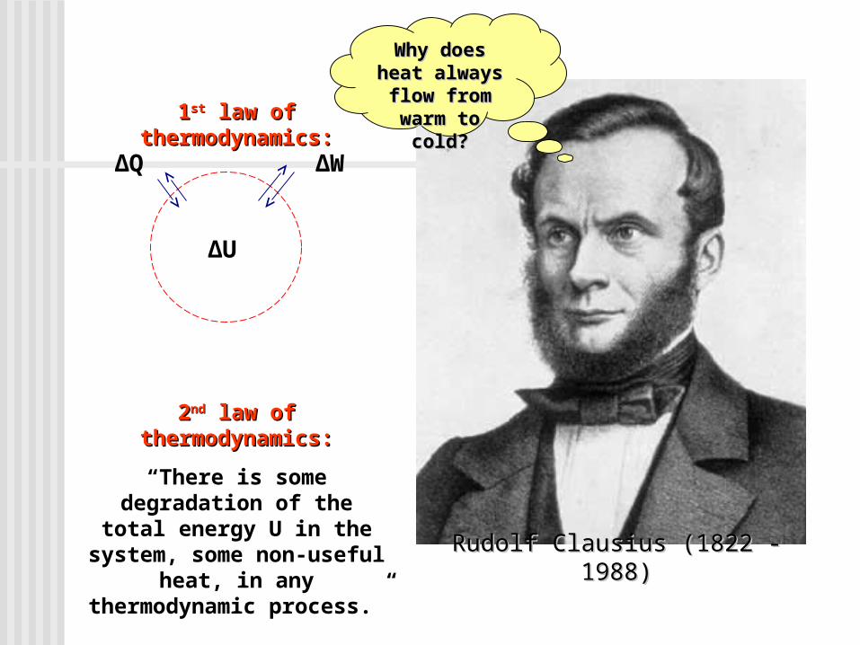
11stst law of thermodynamics: law of thermodynamics:

22ndnd law of thermodynamics: law of thermodynamics:

“There is some degradation of the total energy U in the system,

some non-useful heat, in any thermodynamic process.”

Rudolf Clausius (1822 - 1988)Rudolf Clausius (1822 - 1988)

ΔWΔQ

ΔU

Why does heat Why does heat always flow always flow

from warm to from warm to cold?cold?

Ludwig Boltzmann (1844 - 1906)Ludwig Boltzmann (1844 - 1906)

““When energy is degraded, the When energy is degraded, the atoms become more disordered, atoms become more disordered,

the entropy increases!”the entropy increases!”

““At equilibrium, the system will At equilibrium, the system will be in its most probable state and be in its most probable state and the entropy will be maximum.”the entropy will be maximum.”

The more disordered The more disordered the energy, the less the energy, the less

useful it can be!useful it can be!

WkS log

All possible microstates of 4 coinsAll possible microstates of 4 coins

Three heads, Three heads, one tailsone tails

Two heads, Two heads, two tailstwo tails

One heads, One heads, three tailsthree tails

Four Four headsheads

Four Four tailstails

1W

4W

6W

4W

1W

Boltzmann statistics – 5 dipoles in external field

kT

P0

exp0E ,1 g

kT

UP exp5

1,4UE ,5 ,14 g

kT

UP

2exp10

2,32UE ,10 ,23 g

kT

UP

3exp10

3,23UE ,10 ,32 g

kT

UP

4exp5

4,14UE ,5 ,41 g

kT

UP

5exp55UE ,1 g

E

if , if 0 UEE

General Relations of Boltzmann statisticsGeneral Relations of Boltzmann statistics

– For a system in equilibrium at temperature T:

– Statistical entropy:

i

ii

nn

n

kT

Eg

kT

Eg

Pexp

exp

ii

i PPkS ln

Theoretical Background

The density matrix ρ

– In most cases we do NOTNOT completely know the exact state of the system. We can estimate the probabilities Pi that the system is in the states |ψi>.

– Our system is in an “ensemble” of pure states {Pi,|ψi>}.

inii

iinii

iinii

iniii

iii

iiii

iniii

iiii

iii

niii

ni

i

i

iiiii

aPaaPaaP

aaPaPaaP

aaPaaPaP

aaa

a

a

a

PP

2*2

*1

*2

2

2*12

*1

*21

2

1

**2

*1

2

1

tr(ρ)=1

Define:

Properties of the density matrix– tr(ρ)=1– ρ is a positive operator

(positive, means is real, non-negative, ) – if a unitary operator U is applied, the density matrix

transforms as:

– ρ corresponds to a pure statepure state, if and only if:

– ρ corresponds to a mixed statemixed state, if and only if:

vv v

UtUt 12

1)( 2 tr

1)( 2 tr

– if we choose the energy eigenfunctions for our basis set, then H and ρ are both diagonaldiagonal, i.e.

– in any other representation ρ may or may not be diagonal, but generally it will be symmetricsymmetric, i.e.

Detailed balanceDetailed balance is essential so that equilibrium is maintained (i.e. probabilities do NOT explicitly depend on time).

mnnmnmnnmn EH ,ˆ

nmmn

The reduced density matrix– What happens if we want to describe a subsystem of What happens if we want to describe a subsystem of

the composite system?the composite system?– Divide our system AB into parts A, B.– Reduced density matrix for the subsystem A:

where trB: “partial trace over subsystem B”

)( ABB

A tr

)()( 21212121 bbtraabbaatrB

trace over subspace of system Btrace over subspace of system B

Shannon’s entropy Definition

– How much information we gain, on average, when we How much information we gain, on average, when we learn the value of a random variable X?learn the value of a random variable X?

OR equivalently,

What is the uncertainty, on average, about X before we What is the uncertainty, on average, about X before we learn its value?learn its value?

– If {p1, p2, …,pn} the probability distribution of the n possible values of X:

(bits) log,,, 221 ii

in pppppHXH

– By definition: 0log20 = 0

(events with zero probability do not contribute to entropy.)

– Entropy H(X) depends only on the respective probabilities of the individual events Xi !

– Why is the entropy defined this way? Why is the entropy defined this way?

It gives the minimal physical resources required to store information so that at a later time the information can be reconstructed.

- “Shannon’s noiseless coding theorem”“Shannon’s noiseless coding theorem”..

– Example of Shannon’s noiseless coding theorem Code 4 symbols {1, 2, 3, 4} with probabilities {1/2, 1/4, 1/8, 1/8}.

Code without compression:

But, what happens if we use this code instead?But, what happens if we use this code instead?

Average string length for the second code:

Note:Note: !!!!!!

11,10,01,00 4,3,2,1 compr.without

111,110,10,0 4,3,2,1 compr.with

24

73

8

13

8

12

4

11

2

1lenght

4

7

8

1log

8

2

4

1log

4

1

2

1log

2

1

8

1,

8

1,

4

1,

2

1222

H

Joint and Conditional Entropy– A pair (X,Y) of random variables.– Joint entropy of X and Y:

– Entropy of X conditional on knowing Y:

Mutual Information– How much do X, Y have in common?How much do X, Y have in common? – Mutual information of X and Y:

),(log),(,,

2 yxpyxpYXHyx

YHYXHYXH ,|

YXHYHXHYXH ,:

– , equality when Y= f(X)

– Subadditivity: ,

equality when X, Y are independentindependent variables.

YXHXH ,

YHXHYXH ,

H(X|Y)

H(X) H(Y)

H(Y|X)H(Y:X)

Entropy in the quantum world

Von Neumann’s entropy

– Probability distributions replaced by the density matrix ρ. Von Neumann’s definition:

– If λi are the eigenvalues of ρ, use the equivalent definition:

2logtrS

i

iiS 2log

Basic properties of Von Neumann’s entropy

– , equality if and only if in “pure state”.

– In a d-dimensional Hilbert space: ,

the equality if and only if in a completely mixed statecompletely mixed state, i.e.

– If system AB in a “pure state”, then:

0S

dS 2log

d

d

d

d

I

/100

0/10

00/1

BSAS

– Triangle inequality and subadditivity:

with

Both these inequalities hold for Shannon’s entropy H.

ABB

AA trtrAS A2 , log

BSASBAS

BSASBAS

,

,

ABA

BB trtrBS B2 , log

BAABBSASBAS ,

– Strong subadditivity

First inequality also holds for Shannon’s entropy H, since:

BUTBUT, for Von Neumann’s entropy it is possible that:

However, somehow nature “conspires” so that both of nature “conspires” so that both of these inequalities are NOT true simultaneously!these inequalities are NOT true simultaneously!

CBSBASBSCBAS ,,,,

CBSCASBSAS ,,

CBHBHCAHAH , , ,

CBSBSCASAS ,or ,

Applications

Entropy as a measure of entanglement– Entropy is a measure of the uncertainty about a quantum

system before we make a measurement of its state.– For a d-dimensional Hilbert space:

dS 2log0

Pure state Completely mixed state

– Example:

Consider two 4-qbit systems with initial states:

Which one is more entangled ?Which one is more entangled ?

2

111100001

6

1100101010010110010100112

– Partial measurement randomizesrandomizes the initially pure states.

– The entropy of the resulting mixed states measures the amount of this randomization!

– The largerlarger the entropy, the more randomizedmore randomized the state after the measurement is, the more entangledmore entangled the initial state was!

– We have to go through evaluating the density matrix of the randomized states:

iii

iP

– System 1:System 1:

Trace over (any) 1 qbit:

Trace over (any) 2 qbits:

2

111100001

0111111112

100001111

2

1

111100002

100000000

2

1

S

11111112

1000000

2

133 S

1

21000

0000

0000

00021

22

S

Pure state

λ1,2=0 , λ3,4=1/2

Trace over (any) 3 qbits:

Summary:Summary:

1. initially

2. measure (any) 1 qbit

3. measure (any) 2 qbits

4. measure (any) 3 qbits

1210

02111

S

0S

1S

λ1,2=1/2

– System 2:System 2:

Trace over (any) 1 qbit:

6

1100101010010110010100112

6

110010101001011001010011

6

110010101001011001010011

1

3

100010001

3

100010001

2

1

3

110101011

3

110101011

2

1

3

3

S diagonal

Trace over (any) 2 qbits:

Trace over (any) 3 qbits:

252.13

2log

3

2

6

1log

6

1

6

1log

6

1

61000

031310

031310

00061

2222

2

S

λ1=0, λ2,3=1/6, λ4=2/3

1210

02111

S

λ1,2=1/2

Summary:Summary:

1. initially

2. measure (any) 1 qbit

3. measure (any) 2 qbits

4. measure (any) 3 qbits

Therefore, ψψ22 is more entangled than is more entangled than ψψ11.

0S

1S

252.1S

1S

“ “Ludwin Boltzmann, who spent much of his life studying Ludwin Boltzmann, who spent much of his life studying statistical mechanics, died in 1906, by his own hand. Paul statistical mechanics, died in 1906, by his own hand. Paul Ehrenfest, carrying on the work, died similarly in 1933. Now it is Ehrenfest, carrying on the work, died similarly in 1933. Now it is our turn to study statistical mechanics.”our turn to study statistical mechanics.”

- “States of Matter”, D. Goodstein- “States of Matter”, D. Goodstein

References

“Quantum Computation and Quantum Information”, Nielsen & Chuang, Cambridge Univ. Press, 2000

“Quantum Mechanics”, Eugen Merzbacher, Wiley, 1998

Lecture notes by C. Monroe (PHYS 644, Univ. of Michigan) coursetools.ummu.umich.edu/2001/fall/physics/644/001.nsf

Lecture notes by J. Preskill (PHYS 219, Caltech) www.theory.caltech.edu/people/preskill/ph229