entanglement and quantum error correction with superconducting
TRANSCRIPT

Entanglement and Quantum Error Correction with
Superconducting Qubits
A DissertationPresented to the Faculty of the Graduate School
ofYale University
in Candidacy for the Degree ofDoctor of Philosophy
byMatthew David Reed
Dissertation Director: Professor Robert J. Schoelkopf
May 2013

© 2013 by Matthew David ReedAll rights reserved.
Entanglement and Quantum Error Correction with Superconducting QubitsMatthew David Reed
2013
A quantum computer will use the properties of quantum physics to solve certaincomputational problems much faster than otherwise possible. One promising potentialimplementation is to use superconducting quantum bits in the circuit quantum electro-dynamics (cQED) architecture. There, the low energy states of a nonlinear electronicoscillator are isolated and addressed as a qubit. These qubits are capacitively coupledto the modes of a microwave-frequency transmission line resonator which serves as aquantum communication bus. Microwave electrical pulses are applied to the resonatorto manipulate or measure the qubit state. State control is calibrated using diagnosticsequences that expose systematic errors. Hybridization of the resonator with the qubitgives it a nonlinear response when driven strongly, useful for amplifying the measurementsignal to enhance accuracy. Qubits coupled to the same bus may coherently interactwith one another via the exchange of virtual photons. A two-qubit conditional phasegate mediated by this interaction can deterministically entangle its targets, and is used togenerate two-qubit Bell states and three-qubit GHZ states. These three-qubit states areof particular interest because they redundantly encode quantum information. They are thebasis of the quantum repetition code prototypical of more sophisticated schemes requiredfor quantum computation. Using a three-qubit Toffoli gate, this code is demonstratedto autonomously correct either bit- or phase-flip errors. Despite observing the expectedbehavior, the overall fidelity is low because of decoherence. A superior implementationof cQED replaces the transmission-line resonator with a three-dimensional box mode,increasing lifetimes by an order of magnitude. In-situ qubit frequency control is enabledwith control lines, which are used to fully characterize and control the system Hamiltonian.

Contents
Contents v
List of Figures xi
List of Tables xv
Acknowledgements xvii
Publication list xxi
Nomenclature xxiii
1 Introduction 11.1 Overview of thesis . . . . . . . . . . . . . . . . . . . . . . . . . . . . . 5
2 Concepts of Quantum Information 92.1 Fundamental concepts . . . . . . . . . . . . . . . . . . . . . . . . . . . 11
2.1.1 Single-qubit states . . . . . . . . . . . . . . . . . . . . . . . . . 112.1.2 Single-qubit gates and the Pauli matrices . . . . . . . . . . . . . 122.1.3 Measurement . . . . . . . . . . . . . . . . . . . . . . . . . . . . 142.1.4 Multiple qubits . . . . . . . . . . . . . . . . . . . . . . . . . . . 152.1.5 The density matrix . . . . . . . . . . . . . . . . . . . . . . . . . 172.1.6 Entanglement . . . . . . . . . . . . . . . . . . . . . . . . . . . 21
2.2 Computing with qubits . . . . . . . . . . . . . . . . . . . . . . . . . . . 242.2.1 Quantum algorithms . . . . . . . . . . . . . . . . . . . . . . . . 252.2.2 DiVincenzo criteria . . . . . . . . . . . . . . . . . . . . . . . . . 25
2.3 Quantum errors and error correction . . . . . . . . . . . . . . . . . . . . 29
v
CONTENTS vi
2.3.1 Classical vs. quantum errors . . . . . . . . . . . . . . . . . . . . 292.3.2 The classical repetition code . . . . . . . . . . . . . . . . . . . . 312.3.3 The challenges of quantum errors . . . . . . . . . . . . . . . . . 322.3.4 The quantum repetition code . . . . . . . . . . . . . . . . . . . 342.3.5 The Shor code . . . . . . . . . . . . . . . . . . . . . . . . . . . 412.3.6 Fault tolerance . . . . . . . . . . . . . . . . . . . . . . . . . . . 43
2.4 Conclusions . . . . . . . . . . . . . . . . . . . . . . . . . . . . . . . . . 44
3 Superconducting Qubits and cQED 473.1 Superconducting qubits . . . . . . . . . . . . . . . . . . . . . . . . . . 49
3.1.1 The Transmon qubit . . . . . . . . . . . . . . . . . . . . . . . . 503.1.2 Flux noise . . . . . . . . . . . . . . . . . . . . . . . . . . . . . 57
3.2 Circuit quantum electrodynamics . . . . . . . . . . . . . . . . . . . . . 583.2.1 Harmonic oscillators . . . . . . . . . . . . . . . . . . . . . . . . 593.2.2 Qubit-cavity coupling . . . . . . . . . . . . . . . . . . . . . . . 623.2.3 Dispersive limit and qubit readout . . . . . . . . . . . . . . . . . 643.2.4 Single-qubit gates . . . . . . . . . . . . . . . . . . . . . . . . . 673.2.5 Qubit-qubit coupling . . . . . . . . . . . . . . . . . . . . . . . . 693.2.6 Dissipation and the strong dispersive limit . . . . . . . . . . . . 70
3.3 Flux bias lines . . . . . . . . . . . . . . . . . . . . . . . . . . . . . . . 713.3.1 Flux coupling . . . . . . . . . . . . . . . . . . . . . . . . . . . . 733.3.2 Relaxation through capacitive coupling to FBLs . . . . . . . . . 753.3.3 Filtering . . . . . . . . . . . . . . . . . . . . . . . . . . . . . . 76
3.4 Conclusions . . . . . . . . . . . . . . . . . . . . . . . . . . . . . . . . . 78
4 Experimental Design and Setup 814.1 Planar design . . . . . . . . . . . . . . . . . . . . . . . . . . . . . . . . 82
4.1.1 Planar fabrication . . . . . . . . . . . . . . . . . . . . . . . . . 844.1.2 Planar sample holders . . . . . . . . . . . . . . . . . . . . . . . 85
4.2 Tunable 3D architecture . . . . . . . . . . . . . . . . . . . . . . . . . . 864.2.1 Tunable 3D cQED assembly . . . . . . . . . . . . . . . . . . . . 884.2.2 Cavity design . . . . . . . . . . . . . . . . . . . . . . . . . . . . 914.2.3 Octobox design . . . . . . . . . . . . . . . . . . . . . . . . . . 924.2.4 Qubit design . . . . . . . . . . . . . . . . . . . . . . . . . . . . 954.2.5 Flux bias line design . . . . . . . . . . . . . . . . . . . . . . . . 97
4.3 Dilution fridges and wiring diagram . . . . . . . . . . . . . . . . . . . . 994.4 Pulse generation at room temperature . . . . . . . . . . . . . . . . . . 103
4.4.1 Calibrating the mixer . . . . . . . . . . . . . . . . . . . . . . . . 1044.4.2 Assembly and reflections . . . . . . . . . . . . . . . . . . . . . . 109
4.5 Conclusions . . . . . . . . . . . . . . . . . . . . . . . . . . . . . . . . . 111

CONTENTS vii
5 Single Qubit Gates 1135.1 Experimental bring-up . . . . . . . . . . . . . . . . . . . . . . . . . . . 114
5.1.1 Cavity transmission . . . . . . . . . . . . . . . . . . . . . . . . 1145.1.2 Spectroscopy . . . . . . . . . . . . . . . . . . . . . . . . . . . . 117
5.2 Single-qubit pulse tune-ups . . . . . . . . . . . . . . . . . . . . . . . . 1215.2.1 Rabi . . . . . . . . . . . . . . . . . . . . . . . . . . . . . . . . 1215.2.2 Ramsey . . . . . . . . . . . . . . . . . . . . . . . . . . . . . . . 1235.2.3 AllXY . . . . . . . . . . . . . . . . . . . . . . . . . . . . . . . . 1245.2.4 Future tune-up sequences . . . . . . . . . . . . . . . . . . . . . 131
5.3 Summary . . . . . . . . . . . . . . . . . . . . . . . . . . . . . . . . . . 132
6 Qubit Measurement 1356.1 Dispersive readout . . . . . . . . . . . . . . . . . . . . . . . . . . . . . 1366.2 The Purcell filter . . . . . . . . . . . . . . . . . . . . . . . . . . . . . . 140
6.2.1 The Purcell effect . . . . . . . . . . . . . . . . . . . . . . . . . 1416.2.2 Optimizing dispersive fidelity . . . . . . . . . . . . . . . . . . . 1436.2.3 Purcell filter implementation . . . . . . . . . . . . . . . . . . . . 1446.2.4 Qubit reset . . . . . . . . . . . . . . . . . . . . . . . . . . . . . 1496.2.5 Purcell filter summary . . . . . . . . . . . . . . . . . . . . . . . 152
6.3 Jaynes-Cummings readout . . . . . . . . . . . . . . . . . . . . . . . . . 1526.3.1 Cavity nonlinearity . . . . . . . . . . . . . . . . . . . . . . . . . 1536.3.2 Single and multi-qubit measurement . . . . . . . . . . . . . . . 1586.3.3 Theory of the Jaynes-Cummings nonlinearity . . . . . . . . . . . 1666.3.4 JCR summary . . . . . . . . . . . . . . . . . . . . . . . . . . . 168
6.4 Conclusion . . . . . . . . . . . . . . . . . . . . . . . . . . . . . . . . . 170
7 Tripartite Entanglement on Demand 1737.1 Four-qubit cQED device . . . . . . . . . . . . . . . . . . . . . . . . . . 176
7.1.1 Calibrating flux lines and spectroscopy . . . . . . . . . . . . . . 1767.2 Two-qubit phase gates using fast-flux . . . . . . . . . . . . . . . . . . . 179
7.2.1 Adiabatic controlled-phase gate . . . . . . . . . . . . . . . . . . 1817.2.2 Sudden controlled-phase gate . . . . . . . . . . . . . . . . . . . 1877.2.3 Other two-qubit gates . . . . . . . . . . . . . . . . . . . . . . . 193
7.3 State tomography . . . . . . . . . . . . . . . . . . . . . . . . . . . . . 1947.3.1 Errors and physicality of state tomograms . . . . . . . . . . . . . 202
7.4 Process tomography . . . . . . . . . . . . . . . . . . . . . . . . . . . . 2047.5 Entanglement on demand . . . . . . . . . . . . . . . . . . . . . . . . . 207
7.5.1 Entanglement witnesses . . . . . . . . . . . . . . . . . . . . . . 2137.6 Conclusion . . . . . . . . . . . . . . . . . . . . . . . . . . . . . . . . . 217
CONTENTS viii
8 Quantum Error Correction with cQED 2198.1 Toffoli gate . . . . . . . . . . . . . . . . . . . . . . . . . . . . . . . . . 220
8.1.1 Efficient Toffoli using higher levels . . . . . . . . . . . . . . . . . 2228.1.2 |111〉 → |102〉 transfer . . . . . . . . . . . . . . . . . . . . . . . 2238.1.3 |102〉 � |003〉 interaction . . . . . . . . . . . . . . . . . . . . . 2318.1.4 Two-qubit phases . . . . . . . . . . . . . . . . . . . . . . . . . 2338.1.5 Pulse sequence and the cRamsey phase tune-up procedure . . . . 2358.1.6 Toffoli-sign gate tomography . . . . . . . . . . . . . . . . . . . 239
8.2 Realizing the bit-flip code . . . . . . . . . . . . . . . . . . . . . . . . . 2438.2.1 Finite rotation errors . . . . . . . . . . . . . . . . . . . . . . . . 2448.2.2 Verifying ancilla states . . . . . . . . . . . . . . . . . . . . . . . 246
8.3 Realizing the phase-flip code . . . . . . . . . . . . . . . . . . . . . . . . 2488.3.1 Simultaneous errors . . . . . . . . . . . . . . . . . . . . . . . . 2488.3.2 Process tomography . . . . . . . . . . . . . . . . . . . . . . . . 249
8.4 Conclusion . . . . . . . . . . . . . . . . . . . . . . . . . . . . . . . . . 251
9 The Tunable 3D cQED Architecture 2539.1 Qubit lifetimes and FBL filtering . . . . . . . . . . . . . . . . . . . . . 254
9.1.1 Fast flux performance . . . . . . . . . . . . . . . . . . . . . . . 2589.2 Device characterization with Fock states . . . . . . . . . . . . . . . . . 259
9.2.1 System spectrum . . . . . . . . . . . . . . . . . . . . . . . . . . 2609.2.2 Cavity Rabi oscillation . . . . . . . . . . . . . . . . . . . . . . . 2629.2.3 Cavity lifetime . . . . . . . . . . . . . . . . . . . . . . . . . . . 2629.2.4 Cavity coherence . . . . . . . . . . . . . . . . . . . . . . . . . . 2659.2.5 Cavity nonlinearity . . . . . . . . . . . . . . . . . . . . . . . . . 2709.2.6 Cavity dispersive shift . . . . . . . . . . . . . . . . . . . . . . . 272
9.3 Cavity dynamics . . . . . . . . . . . . . . . . . . . . . . . . . . . . . . 2759.3.1 The Husimi Q function . . . . . . . . . . . . . . . . . . . . . . 2759.3.2 Kerr evolution . . . . . . . . . . . . . . . . . . . . . . . . . . . 2769.3.3 Freezing Schrödinger cats . . . . . . . . . . . . . . . . . . . . . 280
9.4 Conclusions . . . . . . . . . . . . . . . . . . . . . . . . . . . . . . . . . 281
10 Conclusions and Future Work 28310.1 Tunable 3D cQED development . . . . . . . . . . . . . . . . . . . . . . 28510.2 Qubit experiments . . . . . . . . . . . . . . . . . . . . . . . . . . . . . 286
10.2.1 Modules . . . . . . . . . . . . . . . . . . . . . . . . . . . . . . 28610.2.2 Multi-cavity experiments . . . . . . . . . . . . . . . . . . . . . . 287
10.3 Outlook on a superconducting quantum computer . . . . . . . . . . . . 290
Bibliography 293
Appendices 319
CONTENTS ix
Appendices 319
A Current-Flux Coupling 319
B Mathematica Code 327
Copyright Permissions 353


List of Figures
2 Concepts of Quantum Information2.1 The Bloch sphere . . . . . . . . . . . . . . . . . . . . . . . . . . . . . 122.2 Classical vs. quantum errors . . . . . . . . . . . . . . . . . . . . . . . . 302.3 Binary symmetric channel . . . . . . . . . . . . . . . . . . . . . . . . . 312.4 Measurement-based QEC circuit . . . . . . . . . . . . . . . . . . . . . . 372.5 Autonomous QEC circuit . . . . . . . . . . . . . . . . . . . . . . . . . 392.6 Nine-qubit Shor code . . . . . . . . . . . . . . . . . . . . . . . . . . . 412.7 Fault-tolerant three-qubit bit-flip code . . . . . . . . . . . . . . . . . . 44
3 Superconducting Qubits and cQED3.1 Transmon energies as a function of gate charge . . . . . . . . . . . . . . 523.2 Transmon eigenstates in the charge basis . . . . . . . . . . . . . . . . . 543.3 Transmon flux tuning as a function of junction asymmetry . . . . . . . . 573.4 cQED eigenenergies . . . . . . . . . . . . . . . . . . . . . . . . . . . . 623.5 Flux bias line designs . . . . . . . . . . . . . . . . . . . . . . . . . . . . 713.6 Flux bias line geometry . . . . . . . . . . . . . . . . . . . . . . . . . . 733.7 Flux bias line circuit . . . . . . . . . . . . . . . . . . . . . . . . . . . . 753.8 Filtered flux bias line circuit . . . . . . . . . . . . . . . . . . . . . . . . 773.9 Qubit lifetime due to flux bias lines with and without filters . . . . . . . 78
4 Experimental Design and Setup4.1 Coplanar waveguide geometry . . . . . . . . . . . . . . . . . . . . . . . 824.2 Four-qubit planar cQED device . . . . . . . . . . . . . . . . . . . . . . 834.3 Planar sample packaging . . . . . . . . . . . . . . . . . . . . . . . . . . 854.4 One- and two-cavity 3D cQED designs . . . . . . . . . . . . . . . . . . 864.5 Single-cavity tunable 3D architecture assembly . . . . . . . . . . . . . . 89
xi

LIST OF FIGURES xii
4.6 Two-cavity 3D octobox assembly . . . . . . . . . . . . . . . . . . . . . 904.7 Tunable single cavity design . . . . . . . . . . . . . . . . . . . . . . . . 914.8 Tunable two-cavity design . . . . . . . . . . . . . . . . . . . . . . . . . 934.9 Octobox design . . . . . . . . . . . . . . . . . . . . . . . . . . . . . . . 944.10 Tunable 3D qubit design . . . . . . . . . . . . . . . . . . . . . . . . . . 954.11 Flux bias line design . . . . . . . . . . . . . . . . . . . . . . . . . . . . 984.12 Diagram of room-temperature electronics and fridge cabling . . . . . . . 1004.13 Typical mixer assembly scheme . . . . . . . . . . . . . . . . . . . . . . 1094.14 Photograph of mixer assembly . . . . . . . . . . . . . . . . . . . . . . . 110
5 Single Qubit Gates5.1 Cavity transmission for various drive strengths . . . . . . . . . . . . . . 1155.2 Transmission vs. applied qubit flux . . . . . . . . . . . . . . . . . . . . 1165.3 Qubit spectroscopy . . . . . . . . . . . . . . . . . . . . . . . . . . . . . 1195.4 Spectroscopy as a function of applied magnetic flux . . . . . . . . . . . 1205.5 Rabi oscillations . . . . . . . . . . . . . . . . . . . . . . . . . . . . . . 1225.6 Experimental and simulated syndromes for amplitude, detuning, and skew-
type errors . . . . . . . . . . . . . . . . . . . . . . . . . . . . . . . . . 1285.7 AllXY reflection error syndrome . . . . . . . . . . . . . . . . . . . . . . 1295.8 DRAG coefficient error syndrome . . . . . . . . . . . . . . . . . . . . . 1305.9 State-dependent Rabi rate . . . . . . . . . . . . . . . . . . . . . . . . . 1315.10 Two-qubit joint AllXY . . . . . . . . . . . . . . . . . . . . . . . . . . . 132
6 Qubit Measurement6.1 Dispersive cavity shift . . . . . . . . . . . . . . . . . . . . . . . . . . . 1386.2 Multi-mode vs single-mode Purcell decay rates . . . . . . . . . . . . . . 1426.3 Design and realization of the Purcell filter . . . . . . . . . . . . . . . . . 1456.4 Diagnostic transmission data of the Purcell filter . . . . . . . . . . . . . 1466.5 Purcell-filtered qubit T1 and comparison to models . . . . . . . . . . . . 1476.6 Calculated Purcell-filtered lifetimes for various filter frequencies . . . . . 1486.7 Fast qubit reset using Purcell filter . . . . . . . . . . . . . . . . . . . . 1506.8 Cavity transmission for low drive strengths . . . . . . . . . . . . . . . . 1546.9 Cavity transmission at large drive strengths and bare cavity response vs.
power . . . . . . . . . . . . . . . . . . . . . . . . . . . . . . . . . . . . 1566.10 Cavity amplitude response . . . . . . . . . . . . . . . . . . . . . . . . . 1576.11 Measurement transients and histograms for single-shot measurement of
one qubit . . . . . . . . . . . . . . . . . . . . . . . . . . . . . . . . . . 1596.12 Measurement histograms and fidelity versus integration time . . . . . . . 1626.13 Pulsed cavity response AH for |111〉 state . . . . . . . . . . . . . . . . . 1646.14 Joint qubit readout fidelity measurement . . . . . . . . . . . . . . . . . 165

LIST OF FIGURES xiii
7 Tripartite Entanglement on Demand7.1 Optical micrograph of the four-qubit cQED device . . . . . . . . . . . . 1757.2 Flux bias line orthogonalization . . . . . . . . . . . . . . . . . . . . . . 1777.3 Fast-flux calibration . . . . . . . . . . . . . . . . . . . . . . . . . . . . 1787.4 Spectroscopic characterization of the four-qubit device . . . . . . . . . . 1797.5 Two-tone spectroscopy of 011-020 avoided crossing . . . . . . . . . . . 1827.6 Conditional frequency shift of |011〉, ζ . . . . . . . . . . . . . . . . . . 1847.7 Model of a sudden approach to an avoided crossing . . . . . . . . . . . 1887.8 Evolution of conditional phase using sudden approach . . . . . . . . . . 1907.9 Swap spectroscopy of 011-002 avoided crossing . . . . . . . . . . . . . . 1917.10 State tomography of separable states . . . . . . . . . . . . . . . . . . . 2007.11 State tomography with population outside the Hilbert space . . . . . . . 2027.12 Process tomography of sudden two-qubit controlled-phase gate . . . . . 2067.13 Circuit model and state tomography of Bell and GHZ states . . . . . . . 2087.14 Calculated separable and entangled state tomograms . . . . . . . . . . . 2107.15 Cityscape density matrix representations of experimentally created states 2127.16 Witnessing entanglement with fidelity and Mermin sum inequalities . . . 2157.17 Witnessing three-qubit entanglement with Mermin product inequalities . 216
8 Quantum Error Correction with cQED8.1 Construction of the ccNOT gate with cNOT gates . . . . . . . . . . . . 2218.2 Calculated spectrum and time-domain measurements of the |111〉 ↔ |102〉
avoided crossing . . . . . . . . . . . . . . . . . . . . . . . . . . . . . . 2248.3 Eigenstate transfer verification test . . . . . . . . . . . . . . . . . . . . 2268.4 Eigenstate transfer verification test with pulse shaping . . . . . . . . . . 2298.5 Calculated spectrum and time-domain measurements of the |102〉 ↔ |003〉
avoided crossing . . . . . . . . . . . . . . . . . . . . . . . . . . . . . . 2308.6 Toffoli-sign pulse sequence . . . . . . . . . . . . . . . . . . . . . . . . . 2368.7 Conditional-Ramsey phase tune-up sequence for measuring φ111 + φ011 . 2388.8 ccNOT implemented with Toffoli-sign gate . . . . . . . . . . . . . . . . 2398.9 ccNOT classical verification state tomograms . . . . . . . . . . . . . . . 2408.10 ccNOT classical truth table . . . . . . . . . . . . . . . . . . . . . . . . 2418.11 Toffoli-sign gate process tomography . . . . . . . . . . . . . . . . . . . 2428.12 Bit-flip QEC circuit . . . . . . . . . . . . . . . . . . . . . . . . . . . . 2438.13 Bit-flip quantum error correction with finite error rotations . . . . . . . . 2458.14 Ancilla states after bit-flip quantum error correction . . . . . . . . . . . 2478.15 Phase-flip quantum error correction circuit . . . . . . . . . . . . . . . . 2478.16 Process tomography of phase-flip quantum error correcting circuit . . . . 250
LIST OF FIGURES xiv
9 The Tunable 3D cQED Architecture9.1 FBL filter performance . . . . . . . . . . . . . . . . . . . . . . . . . . . 2559.2 Fast flux characterization with flux spectroscopy . . . . . . . . . . . . . 2579.3 Flux spectroscopy with 5 ns gaussian pulse width . . . . . . . . . . . . . 2599.4 Qubit spectroscopy as a function of frequency and qubit number splitting
at fmax . . . . . . . . . . . . . . . . . . . . . . . . . . . . . . . . . . . 2609.5 Pulsed spectroscopy of anharmonic cavity . . . . . . . . . . . . . . . . . 2619.6 Cavity Rabi oscillation on 0-1 and 1-2 Fock number states . . . . . . . . 2639.7 Cavity T1 measured with Fock state . . . . . . . . . . . . . . . . . . . . 2649.8 Cavity T1 with qubit moved to its minimum frequency . . . . . . . . . . 2659.9 Cavity T1 as a function of qubit frequency . . . . . . . . . . . . . . . . 2669.10 Cavity T ∗
2 and T echo2 . . . . . . . . . . . . . . . . . . . . . . . . . . . . 267
9.11 Procedure for measuring cavity T2 with the qubit detuned . . . . . . . . 2689.12 Cavity T1 and T2 as a function of qubit frequency . . . . . . . . . . . . 2699.13 Cavity Kerr measurement procedure . . . . . . . . . . . . . . . . . . . . 2719.14 Cavity Kerr as a function of qubit frequency . . . . . . . . . . . . . . . 2729.15 Sequence to measure cavity χ . . . . . . . . . . . . . . . . . . . . . . . 2739.16 Cavity-qubit dispersive shift χ as a function of qubit frequency . . . . . . 2749.17 Q function calibration . . . . . . . . . . . . . . . . . . . . . . . . . . . 2779.18 Procedure for measuring the Q function and example data . . . . . . . . 2789.19 Evolution of a coherent state under the Kerr nonlinearity . . . . . . . . . 2799.20 Freezing Schrödinger cat states with fast flux . . . . . . . . . . . . . . . 281
List of Tables
2 Concepts of Quantum Information2.1 Eigenvalues of the GHZ states . . . . . . . . . . . . . . . . . . . . . . . 36
5 Single Qubit Gates5.1 AllXY pulse sequence . . . . . . . . . . . . . . . . . . . . . . . . . . . 126
7 Tripartite Entanglement on Demand7.1 Gate sequence for one-qubit state tomography . . . . . . . . . . . . . . 1967.2 Gate sequence for two-qubit state tomography . . . . . . . . . . . . . . 1977.3 Gate sequence for three-qubit state tomography, part 1 . . . . . . . . . 1987.4 Gate sequence for three-qubit state tomography, part 2 . . . . . . . . . 199
xv

Acknowledgements
I have had the great fortune to work with some of the smartest and most talented peoplein the world during graduate school. Chief among those I wish to thank is my advisor
Robert Schoelkopf, who is both a world-class scientist and a great mentor. He hastaught me how to be a better researcher and to prioritize the questions and decisions thatmatter now, while disregarding or postponing those that do not. Rob is extremely patient;he allowed me to work on the quantum error correction experiment for months withouttangible results. His confidence in me during that time not only made possible (eventual!)technical and scientific progress, but gave me valuable experience in how to manage sucha large project and better focus my time and energy.
Steve Girvin always made himself available for discussions, despite being in con-tention for the busiest physicist on the planet. His ability to step into a complicatedtechnical discussion and immediately contribute original and innovative ideas was amazing;his intellect and intuition are an inspiration to me.
Michel Devoret has a unique way of approaching problems, distilling even compli-cated and messy ideas down to their (often beautiful) essence. His enthusiasm for andconfidence in the future of quantum information science is a great source of encouragementnot only for the work I did at Yale but also for my career going forward. I admire hismeticulous attention to detail and aesthetic sense, which is refreshing to see in a scientistof his caliber.
Liang Jiang is a much more recent addition to the research effort, but neverthelessmade a big impact for me. His class on quantum information taught me a lot, clarifyingthings that had been a source of confusion for many years. He is a gifted researcher andteacher.
xvii
ACKNOWLEDGEMENTS xviii
The person who I worked closest with in graduate school was Leonardo DiCarlo.I learned from him not only how to run a complicated experiment but also how to approachscientific problems on a practical level. There is no one in the field who works harderthan Leo, which, combined with the fact that he is an outstandingly brilliant scientist,means that he sets the bar for productivity and knowledge. He holds himself to a veryhigh standard in everything he does, a trait which I aspire to adopt for myself. He is a funand friendly person whom I consider to be a good friend.
More recently, I have had the pleasure of working with Kevin Chou, Nissim Ofek,and Jacob Blumoff on the tunable 3D cQED project. Kevin’s boundless enthusiasmand willingness to work late into the night was a big reason for the project’s success. He isa fast learner and was able to rapidly take over the day-to-day operation of the experiment.Nissim’s practicality and causal confidence were also key, as was his considerable skill infabrication, assembly, and programming. Even when other projects were making demandson his time, he was always willing to help with sample assembly or another round offabrication. Jacob took the lead in sorting out some of the most difficult outstandingtheoretical questions about the device, including how to accurately and robustly model avertical transmon qubit and calculate its Purcell relaxation. These tools will be crucial fordesigning the next generation of experiments, which I know I am leaving in capable hands.
This work was conducted on the fourth floor of Becton Center at Yale University, whichhas an amazing collaborative environment. All of the people who have done work on thefourth floor were on some level involved in the work presented in this thesis, but thereare a few I would like to thank in particular. Luigi Frunzio is a staple of the fourthfloor, operating and maintaining much of the fabrication and mechanical equipment weall rely on; he is partly responsible for fabricating many of the devices reported on in thisthesis. He is an ebullient and good-humored person, whose personality perpetuates thegood culture of Becton.
I have learned a lot from both David Schuster and Andrew Houck. Dave is thequintessential physicist who, in addition to having an encyclopedic knowledge of cQED,seems to have a well thought out and compelling opinion about virtually everything fromboard games to domestic policy. Andrew had the original idea of my first project of thePurcell filter and taught me many early skills including how to wirebond. More recently,he has been a great source of advice for planning the next stage of my career. He is anengaging and friendly person, who genuinely cares about the well-being of those aroundhim.
ACKNOWLEDGEMENTS xix
Blake Johnson and Jerry Chow were the senior graduate students when I firstjoined Schoelkopf lab, and were directly involved in training me to run experiments. Blakeincluded me in his pioneering two-cavity experiment, showing me how to run Clean Sweepand the pulse sequencing program. Jerry was similarly helpful in my early days, workingwith me to find my first qubit. Both Jerry and Blake are fun and friendly people withgreat senses of humor.
Luyan Sun, Gerhard Kirchmair, and Michael Hatridge are more recentadditions to Becton, but are also important in the success of my research. Luyan is anamazingly hard-working person who is always willing to help debug the experiment orprovide advice, and is generous with sharing the credit for his success. Gerhard is outgoingand personable, and is consistently enthusiastic and ready to help. He is also incrediblysmart; whenever I explained something and he agreed with me, I knew I must be right. Iconsider him to be good friend, and enjoyed our frequent games of Munchkin. Mike hasa deep knowledge of all aspects of the experimental equipment, from quantum-limitedamplifiers to idiosyncrasies with cryogen-free dilution fridges; he is the guy you go to witha question no one else can answer. He is a fun and welcoming person, and regularly threwsome of the best parties I have been to in recent memory. Hanhee Paik was also akey member of the floor, whose good sense of humor and thoughtfulness brightened theenvironment for everyone.
Teresa Brecht and Brian Vlastakis are valued colleagues and friends. Teresa,whose self-effacing manner belies her remarkable competence and intelligence, holds herselfto higher standard than almost anyone I know. Her enthusiasm and genuine interest inmy work has redoubled my own focus. She is one of my favorite people to hang out with,and we have become close friends. Brian is an outgoing and friendly person who, likeTeresa, does not seem to realize how much cooler he is than everyone else. He was happyto provide a huge amount of help in setting up the Schrödinger cat experiment, and playsa mean game of Munchkin.
Eleanor Sarasohn has become one of my closest friends in my last years ofgraduate school, and is one of the kindest people I have ever met. She is a singularlytalented poet, whose enthusiasm for learning about all manner of topics is infectious. Ican always rely on her for astute and unvarnished opinions and advice. Eleanor has madean indelible change to my life – in particular by helping me to figure out what to do aftergraduate school – and knows me better than almost anyone. She also gave me absurdly
ACKNOWLEDGEMENTS xx
detailed feedback and editorial comments on this thesis, reading the entire documentcover-to-cover twice; it is vastly improved as a result.
During my time at Yale, Devon Cimini has become by best friend. He has a greatsense of humor and is generous with his time and ideas. He is a deeply rational, intelligent,and level-headed person, and is a great source of advice. Devon was always available to talkabout the latest development in politics or technology and offered practical encouragementwhen things in lab were not going well. I will always fondly remember board game nightsand taking turns playing new indie video games in our living room.
I apparently first met Sarah Rusk in college, though neither of us have any recollectionof it; fortunately for me, we reconnected at Yale. Sarah has an excellent sense of humor,is extremely loyal, caring, and understanding and is one of my favorite people and bestfriends. She is also a fantastic cook and has a great appreciation for culture, two propertieswhich I hope to continue to assimilate. I have learned a lot from her about how to be anadult and enjoy life; together we have become connoisseurs of wine costing less than tendollars per bottle. In recent months, she listened to numerous practice job talks and wasinvaluable to me in helping to sort out what I should do after graduating.
Finally, I would like to thank my family Brian Reed, Roberta Reed, and Andrea
Wilson. Their support was essential to me not only in graduate school, but throughoutmy life; I would not have gotten the places I have without it. My father, Brian, got meinterested in science from an early age and encouraged that passion and technical thinking.My mother, Roberta, equipped me with the writing skills that I have relied on heavily.Both parents were supportive of my decision to enroll at Harvey Mudd College, which wasthe more expensive option but created many of the the opportunities that I enjoy today. Iam also particularly thankful to my sister, Andrea, for recently contributing her excellentbusiness sense and advice about my future career.
There are of course countless unnamed others who are owed thanks as well, includingteachers, mentors, professors, and friends.
Publication list
This thesis is based in part on the following publications:
1. M. D. Reed, B. R. Johnson, A. A. Houck, L. DiCarlo, J. M. Chow, D. I. Schuster,L. Frunzio, and R. J. Schoelkopf, “Fast reset and suppressing spontaneous emissionof a superconducting qubit,” Appl. Phys. Lett. 96, 203110 (2010).
2. B. R. Johnson, M. D. Reed, A. A. Houck, D. I. Schuster, L. S. Bishop, E.Ginossar, J. M. Gambetta, L. DiCarlo, L. Frunzio, S. M. Girvin, and R. J.Schoelkopf, “Quantum non-demolition detection of single microwave photons in acircuit,” Nat. Phys. 6, 663–667 (2010).
3. M. D. Reed, L. DiCarlo, B. R. Johnson, L. Sun, D. I. Schuster, L. Frunzio, and R.J. Schoelkopf, “High-fidelity readout in circuit quantum electrodynamics using theJaynes-Cummings nonlinearity,” Phys. Rev. Lett. 105, 173601 (2010).
4. L. DiCarlo, M. D. Reed, L. Sun, B. R. Johnson, J. M. Chow, J. M. Gambetta, L.Frunzio, S. M. Girvin, M. H. Devoret, and R. J. Schoelkopf, “Preparation andmeasurement of three-qubit entanglement in a superconducting circuit,” Nature467, 574–578 (2010).
5. L. Sun, L. DiCarlo, M. D. Reed, G. Catelani, L. S. Bishop, D. I. Schuster, B. R.Johnson, G. A. Yang, L. Frunzio, L. Glazman, M. H. Devoret, and R. J. Schoelkopf,“Measurements of quasiparticle tunneling dynamics in a band-gap-engineeredtransmon qubit,” Phys. Rev. Lett. 108, 230509 (2012).
6. M. D. Reed, L. DiCarlo, S. E. Nigg, L. Sun, L. Frunzio, S. M. Girvin, and R. J.Schoelkopf, “Realization of three-qubit quantum error correction withsuperconducting circuits,” Nature 482, 382–385 (2012).
xxi

Nomenclature
Abbreviations:
APS arbitrary pulse sequencer (section 4.4).
AWG arbitrary waveform generator (section 4.4).
BBQ black-box quantization or barbecue (section 6.3.1).
ccNOT Three-qubit controlled-controlled-NOT gate, also known as Toffoli. (section2.3.4).
CHSH Clauser-Horne-Shimony-Holt (section 7.5.1).
cNOT controlled-NOT gate (section 2.1.4).
CPB Cooper-pair box (section 3.1.1).
cPhase controlled-phase gate (section 2.1.4).
CPW coplanar waveguide (section 4.1).
cQED circuit quantum electrodynamics (section 3.2).
cRamsey Conditional Ramsey sequence, used for measuring conditional phases. (section8.1.5).
CW continuous-wave (section 4.4).
DAC digital to analog converter (section 7.1.1).
DRAG derivative removal by adiabatic gate (section 5.2.3).
EPR Einstein-Podolsky-Rosen (section 1).
FBL flux bias line (section 3.3).
xxiii

NOMENCLATURE xxiv
GHZ-like state of the form α|000〉+β|111〉. GHZ-class when |α| = |β| = 1/√2. (section
2.3.4).
HEMT high electron mobility transistor amplifier (section 6.1).
IQ in-phase / quadrature (section 4.3).
JBA Josephson bifurcation amplifier (section 6.1).
JC Jaynes-Cummings (section 3.2.2).
JPC Josephson parametric converter (section 6.1).
LHV local hidden variable (section 7.5.1).
LO local oscillator (section 4.3).
NMR nuclear magnetic resonance (section 1).
PCB printed circuit board (section 4.1.2).
QEC quantum error correction (section 2.3).
QND quantum non-demolition (section 2.1.3).
RF radio frequency (section 4.3).
RWA rotating wave approximation (section 3.2.2).
SMA sub-miniature version A microwave connector (section 4.2.3).
SNR signal-to-noise ratio (section 6.1).
SQUID superconducting quantum interference device (section 3.1.1).
SSB single sideband modulation or mixing (section 4.4.1).
VSWR voltage standing wave ratio (section 4.4.1).
��
Latin Letters:
a†, a creation and annihilation operators for a resonator (section 3.2.1).
AH averaged homodyne amplitude (section 6.3.1).
b†, b creation and annihilation operators for the qubit in the harmonic approximation(section 3.2.2).
Cq qubit capacitance (section 6.2.1).
CΣ total qubit capacitance to ground (section 3.1.1).
NOMENCLATURE xxv
D harmonic oscillator displacement operator (section 3.2.1).
EC electrostatic charging energy (section 3.1.1).
EJ Josephson energy (section 3.1.1).
EmaxJ maximum value for the effective EJ under flux tuning (section 3.1.1).
fbare bare cavity frequency (section 6.3).
fmax maximum transition frequency of a flux-tunable qubit (section 5.1.2).
g vacuum-Rabi coupling frequency, g = g01 (section 3.2.2).
|GHZ〉 Greenberger-Horne-Zeilinger state. For three qubits, (|000〉+|111〉)/√2 (section2.1.6).
gij transmon dipole coupling energy between charge levels i and j (section 3.2.2).
H Hadamard matrix (section 2.1.2).
H Hamiltonian (section 2.1.2).
Ic Josephson junction critical current (section 3.1).
J virtual photon qubit-qubit swap interaction strength (section 3.2.5).
K cavity Kerr anharmonicity (section 9.2).
LJ Josephson inductance (section 3.1).
M measurement operator (section 7.3).
ng gate charge (section 3.1.1).
n Cooper pair number operator (section 3.1.1).
Q cavity quality factor, also Qtot (section 4.1).
Q1-Q4 qubits in the four-qubit device (section 7.1).
Q(α) Husimi quasi-probability distribution (section 9.3.1).
QC cavity coupling quality factor (section 4.1).
QI cavity internal quality factor (section 4.1).
Rθn rotation operator about the n-axis by an angle θ (section 2.1.2).
T1 qubit relaxation time (section 2.1.5).
T2 qubit dephasing time (section 2.1.5).
T echo2 dephasing time when using a Hahn echo sequence (section 9.2.4).

NOMENCLATURE xxvi
T ∗2 dephasing time when performing a Ramsey measurement (section 9.2.4).
VH homodyne measurement voltage (section 7.3).
|W 〉 W state. For three qubits, (|100〉 + |010〉 + |001〉)/√3 (section 2.1.6).
Y circuit admittance (section 6.2.1).
��
Greek Letters:
α transmon anharmonicity (section 3.1.1).
|α〉 coherent state (section 3.2.1).
β voltage division ratio (section 3.2.2).
γ qubit relaxation rate (section 3.2.6).
γκ Purcell decay rate (section 6.2.1).
Λ(σx) controlled-NOT gate (section 2.1.4).
Λ(σz) controlled-phase gate (section 2.1.4).
Δ qubit-cavity detuning, Δ = ωq − ωr (section 3.2.2).
εeff effective dielectric strength (section 4.1).
ξ two-qubit σz ⊗ σz interaction strength (section 3.2.5).
κ cavity linewidth; photon relaxation rate (section 3.2.2).
ωq qubit transition frequency (section 6.2.1).
ξ external drive strength (section 3.2.4).
ρ density matrix (section 2.1.5).
σi Pauli I matrix (section 2.1.2).
σx Pauli X matrix (section 2.1.2).
σy Pauli Y matrix (section 2.1.2).
σz Pauli Z matrix (section 2.1.2).
Φ0 magnetic flux quantum given by h/2e (section 3.1).
φ junction phase operator (section 3.1.1).
χ state-dependent dispersive cavity shift (section 3.2.2).

NOMENCLATURE xxvii
χij state-dependent dispersive cavity shift with respect to the i to j transmontransition (section 3.2.2).
χmn χ-matrix representation of the quantum process matrix (section 7.4).
ΩR Rabi frequency (section 3.2.4).
ωq qubit ground to excited state transition frequency (section 3.2.2).
ωr resonator transition frequency (section 3.2.2).

CHAPTER 1
Introduction
At the turn of the twentieth century, it was widely believed that physics was complete.Electricity and magnetism were unified with Maxwell’s equations, statistical mechanics
accurately predicted the properties of fluids and gases, and optics, acoustics, thermody-namics, and kinetics all seemed to be understood. This was reflected in the progressof the industrial revolution. Steam power, transatlantic radio, and the telegraph weredirect results of physical understanding, yet several nagging problems remained. In 1895,Wilhelm Röntgen created x-rays and in 1889, Marie Curie discovered radiation, neitherof which had an explanation. In 1902, Philipp Lenard observed that the photoelectricvoltage depended on the color of light and not its intensity, to the contrary of Maxwell’spredictions. The Rayleigh law of 1900 absurdly predicted that a black body at thermalequilibrium will emit radiation with infinite power at short wavelengths, a problem knownas the ultraviolet catastrophe. And in 1911, Ernest Rutherford showed that electrons orbitthe tiny positively-charged nucleus of the atom, but could not explain why the electronsdo not fall in.
Initially, a few postulates were used to rectify these problems. In 1900, Max Plancksuggested that energy was quantized and that light came in integer units of hν, where ν isthe frequency of the light and h is a number known as Planck’s constant. This conjecturesolved the problem of black body radiation, but its broader implications were unappreciated
1
CHAPTER 1. INTRODUCTION 2
until much later. In 1905, Albert Einstein explained the photoelectric effect with this ideaof energy quantization. In 1913, Neils Bohr suggested that electrons orbiting atoms couldonly occupy certain well-defined orbitals, which explained why electrons did not spiral intoan atomic nucleus as well as why atoms emitted only at discrete energy levels. Thesetheories, despite remaining strictly phenomenological, successfully explained many of thespecific experimental difficulties of the age. However, this “old quantum theory” offeredno justification for quantization nor underlying structure.
It was not until 1925 that a modern theory of quantum mechanics was developed.Werner Heisenberg and Erwin Schrödinger invented respectively, matrix mechanics andwave mechanics. Although this modern theory unified the phenomenological postulates, ithad bizarre implications. Particles could be in more than one state at once and propertieslike position and momentum could not be simultaneously known. Even determinism– arguably the deepest postulate of modern science – would be thrown out. For thisreason, and despite its success at explaining the world, the modern theory had numerousdetractors. Albert Einstein, Boris Podolsky, and Nathan Rosen highlighted a supposedparadox that occurred when two “entangled” particles were separated and one measured[1]. The information of this measurement appeared to be instantly transmitted to theunmeasured particle regardless of distance, which seemed to violate the special theoryof relativity. EPR suggested that the only resolution to this problem was that quantumtheory was incomplete.
Despite this and other vociferous challenges, quantum theory was simply too effectiveto repudiate. It accurately and self-consistently described the world, especially afterthe development of renormalized quantum field theory that unified special relativity andquantum physics in the early 1950’s [2]. For example, field theory correctly predictsthe electron spin g-factor to a precision of better than one part per trillion [3, 4]. Therelativistic objections to quantum mechanics were also dismissed, most famously by JohnBell’s theorem of 1964 [5]. Bell showed that there are physical consequences of quantumentanglement which could not occur if “local hidden variables” pre-ordained particlecorrelations. The subsequent experimental verification of this theorem by Alain Aspect in1981 [6] and others proved that the universe truly disobeyed local realism.
The development of Bell’s theorem greatly strengthened the conceptual foundationof quantum theory, but fundamental questions about the nature of quantum informationremained. For example, could entanglement be used to transmit information faster thanthe speed of light? This question∗ led to the development of the No-Cloning Theorem
CHAPTER 1. INTRODUCTION 3
[7], which held that an arbitrary quantum state could not be perfectly copied and thusentanglement could not violate relativity. Proposals for forgery-proof quantum money [8]and provably secure communication using quantum key distribution [9] were made as adirect result.
These developments raised the question of whether the properties of quantum mechanicscould be leveraged for other useful purposes. In 1982, Richard Feynman suggested thata computer using quantum mechanics might more naturally model the physical world[11]. David Deutsch showed in 1985 that such a “quantum computer” could not beefficiently simulated with a classical one, which cemented the supposition that quantuminformation is fundamentally different from its classical counterpart [12]. Initially, thiswas only of theoretical interest since it was unclear how to actually achieve a quantumspeed-up. Though the state of a quantum computer could evolve in a huge parallelsuperposition, the result of a computation would be randomly chosen from that populationwhen it was measured. Fortunately, the Deutsch-Jozsa algorithm was discovered in 1992,demonstrating that this was a surmountable problem [13]. Though that algorithm haslittle practical use, it runs exponentially faster than any classical solution and provedthat, in principle, the computational power of quantum physics could be accessed. Moreimportantly, Peter Shor discovered an integer factoring algorithm in 1995 which could alsorealize an exponential speed-up [14]. The computational difficulty of factorizing numbersis the basis of many classical encryption algorithms [15], so an efficient algorithm providedsignificant motivation for further study of quantum information science.
For the same reason that a quantum computer would be powerful, it would also behighly susceptible to errors. Quantum bits are intrinsically analog devices and are describedby continuous variables. Any spurious interactions with the environment or imprecisionin control signals will cause the quantum state to become corrupted. Moreover, even ifeach individual error is small, there is nothing to prevent subsequent errors from buildingup and propagating as an algorithm is run. Thus, the rate at which errors occur sets afundamental limit on the duration of a calculation that has any appreciable chance ofsuccess, and is quite low for a calculation of any size. For example, the rate required to
∗ These questions had long been disregarded by the mainstream community, who largely adhered to the“shut up and calculate” school of quantum-mechanical thought. However, a group of counter-culture BayArea physicists in the 1970’s who failed to find jobs following the postwar physics boom formed a cohortto investigate these more philosophical questions. Their “Fundamental Fysiks Group” proposed a methodof transmitting information faster than the speed of light, which three groups independently discoveredthe No-Cloning theorem to resolve [10].
CHAPTER 1. INTRODUCTION 4
run Shor’s algorithm on an appreciably large number is ten or more orders of magnitudelower than could ever feasibly be achieved [16]. Without some means of circumventingthis issue, the quantum computer would again be relegated to a mere theoretical curiosity.Fortunately, in 1995 Peter Shor proposed the first “quantum error correction” code, bywhich a single “logical” qubit was redundantly encoded with nine physical qubits [17]. Thiscode makes the effective error rate of a logical qubit much lower than the rates of eachconstituent qubit. Error correcting codes requiring 5 or 7 qubits were discovered shortlythen after [18, 19], but merely correcting errors is not enough to compute. These logicalqubits must be usable in algorithms, which means manipulating them in a way that isrobust to errors as well. Peter Shor once again solved this problem∗, finding in 1996 thatan arbitrarily perfect fault tolerant quantum computer could be built from faulty qubits[20].
With a quantum computer shown to be theoretically possible, it turned to experimentalgroups to attempt to build one. The earliest efforts used liquid-state nuclear magneticresonance (NMR). Due to its applications to medicine and chemistry, NMR alreadyhad some of the necessary functionality, such as single-qubit gates and good coherencetimes. For that reason, initial progress was rapid with demonstrations of simple two-qubitalgorithms [21–23] soon followed by a seven-qubit factorization of the number 15 usingShor’s algorithm [24]. For a variety of reasons including poor measurement signal-to-noiseand register initialization, however, liquid-state NMR could not scale much past this point[25].
A more promising approach was to use trapped ions [26]. In that system, a linearstring of ionized beryllium, calcium, strontium, or another type of atom are confined usingelectric fields. Certain electronic transitions of each atom are used as a qubit, with highertransitions used for measurement and initialization [27]. Ions are coupled to one anotherby their collective motion, which is essentially a coherent “phonon bus.” High-precisionlasers are used for both single and multi-qubit manipulations†. The field also enjoyed briskprogress by leveraging the techniques and machinery developed for atomic clocks, and bytaking advantage of the long coherence times of atomic transitions [28–31]. This systemcurrently holds the record for measurement [32] and gate fidelity [33], as well as for themost qubits simultaneously controlled (fourteen) [34]. Despite this, scaling to thousands
∗ It is rather remarkable that the same person discovered the most important algorithm and solved the twobiggest theoretical challenges facing quantum information.
CHAPTER 1. INTRODUCTION 5
or millions of trapped ions is an imposing problem. Correlated noise [34] harms statefidelity as the system grows, and the experimental apparatus required for these relativelysmall systems are quite complicated. Progress has been made toward miniaturizing thetrap onto a chip [35, 36], but combining the huge current required to trap ions with theconstraints of a cryogenic circuit represents a challenge [37].
A variety of other quantum computing systems have recently been introduced. Someexamples of credible architectures are optical lattices of neutral atoms [39], semiconductorquantum dots [40–44], electrons trapped over liquid helium [45], and diamond nitrogen-vacancy centers [44, 46–48]. One of the most promising new approaches and the subjectof this thesis is superconducting circuits [49]. There, the collective motion of Cooper pairsin a nonlinear electronic circuit is quantized and used as a qubit [50–52]. The state of thismotion can be controlled and detected with microwave signals. Superconducting circuitshave been used to demonstrate a variety of quantum information tasks like single-qubitgates [53, 54], two-qubit gates [55–57] and high-fidelity measurement [58–61]. For muchof their history, however, there was an open question about whether these circuits couldbe sufficiently coherent to attain fault tolerance. Fortunately, in the context of very recentexperiments [62, 63], it appears that the answer is yes.
1.1 Overview of thesis
This thesis reports recent results using the circuit quantum electrodynamics (cQED)superconducting architecture. This system, in which superconducting qubits are coupledto microwave cavities, has proven itself as one of the most promising implementations ofsuperconducting technology and potentially of any known quantum computing architecture.I begin by introducing the characteristics and experimental implementation of cQED andculminate with the experimental realization of the three-qubit quantum error correctingcode. A variety of other results will also be reported, including a new mechanism forqubit readout and a design for improving the coherence of qubits without sacrificingcontrollability.
† This fact is amusing in the context of a quote from Erwin Schrödinger in 1952, where he said that“we never experiment with just one electron or atom or (small) molecule. In thought-experiments wesometimes assume that we do; this invariably entails ridiculous consequences... we are not experimentingwith single particles any more than we can raise Ichthyosauria in the zoo” [38]. The Ichthyosaur is adolphin-like marine reptile that has been extinct for 90 million years.
CHAPTER 1. INTRODUCTION 6
Before examining the details of the system, I provide a brief overview of quantuminformation science in chapter 2. I introduce the concept of quantum bits, gates, algorithms,and measurement. I discuss entanglement and how it can be quantified, and briefly mentionthe requirements for a quantum computer and a few useful algorithms that can be run onone. The chapter concludes by emphasizing the need for quantum error correction andlisting several approaches to do so.
In chapter 3, I summarize the physics of these superconducting systems. I introducethe transmon qubit, which is the qubit variant used throughout this thesis, and show howit can be coupled to a microwave resonator in cQED. Control of the resonator enables usto apply single-qubit gates, mediate coupling between qubits, and measure qubit states. Idiscuss flux bias lines, which are used to control qubit transition frequencies in-situ, andshow how to calculate the expected qubit relaxation.
With the theoretical concepts established, I turn to the details of our experimentalimplementation in chapter 4. I introduce two approaches to building cQED: the two-dimensional planar design and the three-dimensional cavity design. Though they areconceptually similar, their designs are quite different. I show a new variant on 3D cavitiesthat integrates flux bias lines and comes with its own host of design considerations. I thenexplain how the devices are cooled in a helium dilution refrigerator, and describe how thefridge is cabled to maximize thermalization, control precision, and measurement fidelity.Finally, I explain how single-qubit gates are accurately and inexpensively generated at roomtemperature.
Calibrating these gates in a real experiment is the subject of chapter 5. I introducesimple procedures for measuring cavity transmission and qubit spectroscopy which arerequired to initiate any cQED experiment. I then show how to progressively tune-up qubitpulses with Rabi and Ramsey oscillations and a sequence called “AllXY.” This sequenceis more sensitive to a variety of pulse error syndromes than other approaches, and is anarchetype for even more sophisticated tune-ups.
Chapter 6 concerns the details of qubit measurement. It begins with the conventionaldispersive mechanism and calculates the expected signal to noise ratio of such a mea-surement. Due to the low signal power and the relatively high noise temperature of theamplifier chain most often used, this SNR and the corresponding measurement fidelitycan be low. Motivated by this fact, I introduce a new element called a “Purcell filter”that breaks the relationship between qubit and cavity lifetime. Apart from enabling theuse of low-Q measurement cavities to increase dispersive measurement fidelity, it can
CHAPTER 1. INTRODUCTION 7
also be used to efficiently reset qubits to their ground state. I then discuss the “highpower” readout scheme, which exploits the unusual behavior of the cavity when drivenvery strongly to make a high-fidelity measurement. This has the advantage of obviatingthe need for sophisticated amplifiers or design complications to attain good measurementfidelity, but scrambles the qubit state during the measurement, which limits the scope ofits application.
I then turn to more sophisticated qubit experiments and discuss how we have generatedthree-qubit entanglement on demand in chapter 7. I start by describing the characteristicsof the device we used, which hosts four individually flux-biased transmon qubits. I showtwo ways that we can use this flux control to implement two-qubit entangling gates. Bothmethods exploit an interaction with higher transmon excited states, but approach it eitherin the slow (adiabatic) or fast (sudden) limit. In order to verify that these gates are workingas expected and to quantify their fidelity, I discuss how state and process tomography canbe efficiently measured with a joint qubit measurement. Finally, using the sudden two-qubitgate, I explain how we have produced three-qubit entanglement and measured the resultingstate with tomography. We also verified the presence and quality of entanglement withvarious witnesses.
These techniques lead directly into chapter 8, where I discuss our recent demonstrationof three-qubit quantum error correction. The key to this result is an efficient three-qubitToffoli gate. This gate leverages our understanding of both sudden and adiabatic gatesusing higher-excited states to engineer an interaction between a computational state and athird-excited state of one transmon. I discuss the procedure we have developed to tune thegate up and report the resulting performance as measured by state and process tomography.Using this gate, we demonstrated both bit- and phase-flip quantum error correction. Weverified that the algorithm worked as expected by measuring the ancilla qubit states aftera full bit-flip on a single qubit and confirming the quadratic dependence of fidelity on theeffective error rate of all three qubits. Despite this success, the algorithm never improvesthe fidelity of a process because the coherence of the qubits in the device was too poor.
Motivated by this result and recent breakthroughs in 3D qubit coherence [62, 64],I report on preliminary results using a tunable version of the 3D cQED architecture inchapter 9. I show how the added control lines constitute an unacceptable qubit decaychannel as we expected, and that this channel can be effectively turned off with properfiltering. I then discuss a host of experiments we have performed to measure the systemby combining cavity photon-number Fock states with fast flux control. These techniques
CHAPTER 1. INTRODUCTION 8
enabled us to accurately measure cavity lifetime, coherence, nonlinearity, and dispersiveshift as a function of qubit frequency. These results indicate that, in the absence ofqubit hybridization, the cavity can be extremely coherent. This leads us to study thecavity itself as a quantum resource. I explain how we have used qubit number splitting tomeasure the cavity state and the inherited Kerr nonlinearity to produce interesting statesto detect. Finally, combining this with fast flux control, I show how we can “freeze” thisKerr evolution, effectively controlling the cavity Hamiltonian on demand.
I conclude this thesis in chapter 10 with an overview of the state of the field andsuggestions for future work. In particular, I list a few straightforward improvements thatcould be made to the tunable architecture to enable more sophisticated experiments. Afew of these experiments are also proposed. Finally, I give my perspective on the future ofsuperconducting qubits and their prospects for implementing a quantum computer.
CHAPTER 2
Concepts of Quantum Information
This chapter will serve as an introduction to the core concepts of quantum informationprocessing. There will be three sections. First, we introduce the fundamental building
blocks and language of quantum information starting with qubits and single-qubit rotations.Next, we describe the reasons that quantum information processing is potentially verypowerful, introduce some of the potential applications, and describe what constitutes thebasic requirements for a “real” quantum computer. We then introduce quantum errorcorrection, which is required for the same reasons that a quantum bit is powerful, and givean example with the simple three-qubit code. We will conclude with a brief survey of thedifferent kinds of more sophisticated error-correcting codes.
The first section will begin with the idea of a quantum bit or “qubit,” which is thefundamental building block of quantum information. We will introduce a useful geometricpicture for their quantum state known as the “Bloch sphere,” and single-qubit “quantumgates” used to manipulate that state which can be viewed as rotations about some axisof the Bloch sphere. One convenient way of describing these rotations is with the Paulimatrices, which correspond to full flips about a given axis but can also be applied in smallamounts using matrix exponentiation. Pauli operators are also useful as a language thatdefines observables of quantum states. We then consider what happens when you havemore than one qubit, both how the quantum state of a register is described and how
9
CHAPTER 2. CONCEPTS OF QUANTUM INFORMATION 10
operators are constructed. The consequences of having multiple qubits leads to a discussionof the density matrix. This accounts for the experimental reality that we are only evercontrolling and measuring subsystems that may be coupled with other uncontrolled degreesof freedom. It also enables us to describe the state of an ensemble of identically-preparedqubits that do not remain the same because of noise, control imprecision, and decay.We conclude this section by discussing the entanglement of particles and how it can begenerated and detected.
The second section of this chapter will offer an explanation as to why quantuminformation processing has the potential to be such a powerful tool and what it wouldtake to harness that power. We start with a general explanation of the properties ofquantum information. Because particles can be in superpositions of states, even a relativelysmall number of qubits can encode an enormous amount of information. Moreover,that information can be efficiently manipulated with unitary operations. This leads intoa discussion of quantum algorithms, which are specialized procedures that utilize thiscomplexity to solve certain problems faster than otherwise possible. These algorithmsoperate only with stringent requirements, however, which leads us to the final topic of thissection: the DiVincenzo criteria for a quantum computer. Those criteria constitute thebasic hardware requirements that a quantum computer must satisfy.
The final section will explain why quantum bits are much more susceptible to errorsfor the same reason they are powerful. There are straightforward methods of correctingerrors in classical computers which do not seem to easily generalize to the quantum case.Fortunately, by taking advantage of another resource unique to quantum mechanics –entanglement – we demonstrate how a three-qubit quantum repetition code can be madeto correct for arbitrary bit-rotations of any one qubit. There are two implementationsof this code: one relies on measuring error syndromes and classical logic to detect andcorrect an error; the other implementation combines coherent quantum interactions withnon-unitary qubit reset to autonomously correct errors. Both codes can easily be modifiedto fix phase-flip errors instead of bit-flips, which may be a more common error for certainqubit implementations. A qubit is susceptible to both bit- and phase-flips, however, whichrequire a larger code to repair. One such code which corrects for all possible single-qubiterrors is the nine-qubit Shor code, which is a concatenation of the three-qubit bit- andphase-flip repetition codes. We conclude with a discussion of other kinds of error correctingcodes and the concept of fault tolerance.
CHAPTER 2. CONCEPTS OF QUANTUM INFORMATION 11
2.1 Fundamental concepts
The field of quantum information processing typically concerns systems of one or morequantum bits or qubits. A quantum bit is a much more sophisticated object than itsclassical brother. Whereas a classical bit stores only one bit of information, a qubit stateis described by two real numbers – in some sense, an uncountably infinite amount ofinformation. As if this enormous multiplication were not enough, when we have multiplequbits, the amount of information needed to describe the overall state grows exponentiallyas a function of the number of qubits. This section will introduce the basic tools we useto describe and manipulate this quantum information.
2.1.1 Single-qubit states
A single qubit is a quantum object whose allowed states are either |0〉 or |1〉. These “ground”and “excited” states form what is known as the “computational basis.” Being a quantumobject, superpositions of these states are also allowed: the qubit can be in both statessimultaneously. The quantum state of a single qubit is therefore given by |ψ〉 = α|0〉+β|1〉,where α and β are complex numbers and |α|2 + |β|2 = 1. The probability that the qubit isin its ground state is given by |α|2 (or, equivalently, α∗α, where the star operator indicatesthe complex conjugate), and similarly |β|2 for the excited state. Since α and β are complexnumbers, we can equivalently write |ψ〉 = |α|eiφα |0〉 + |β|eiφβ |1〉.
The Bloch sphere
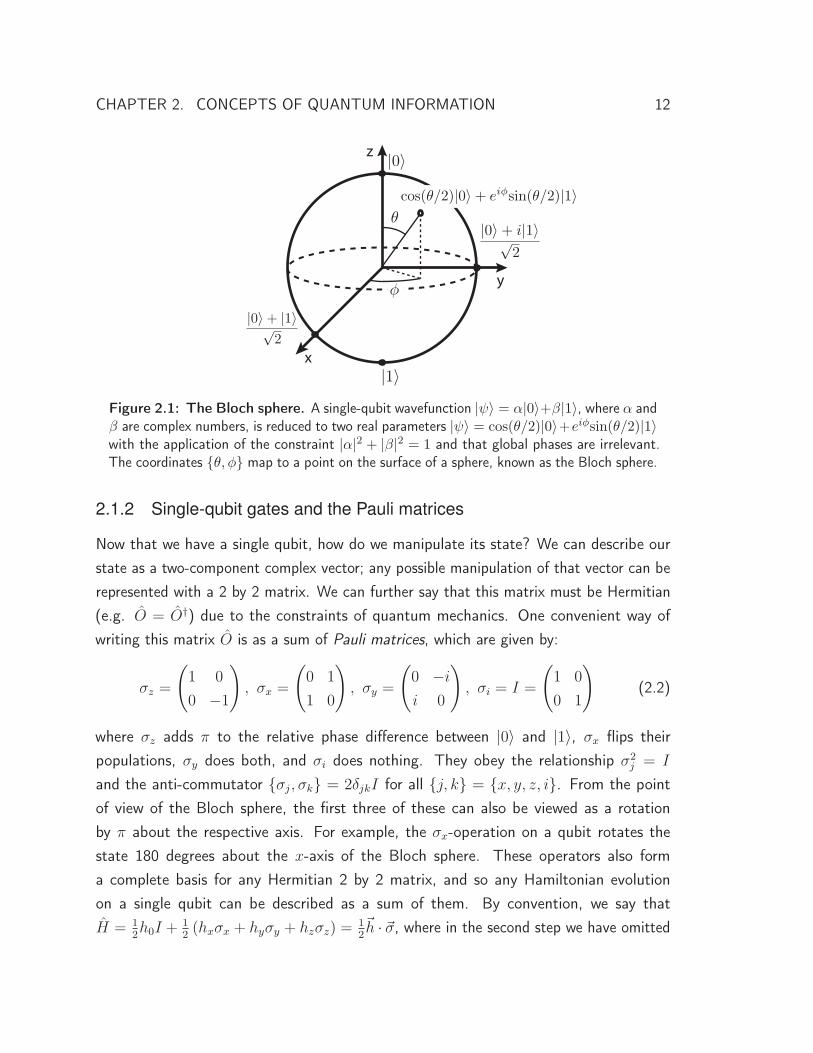
We can further simplify the representation of ψ by exploiting two facts. First, we knowthat the sum of the probability of being found in each state must equal 1, |α|2 + |β|2 = 1.Second, the “global” phase of a quantum state has no physical meaning. Then, definingφ = φβ − φα and noting that cos2(x) + sin2(x) = 1, we say
|ψ〉 = cos
(θ
2
)|0〉 + eiφsin
(θ
2
)|1〉 (2.1)
with θ ∈ [0, π] and φ ∈ [0, 2π). This representation is chosen to map our quantumstate to a point on a sphere, as shown in Fig. 2.1. This is known as the Bloch sphererepresentation of a quantum bit. We can also say that ψ is a two-component vector givenby[cos
(θ2
), eiφsin
(θ2
)].
CHAPTER 2. CONCEPTS OF QUANTUM INFORMATION 12
θ
φ
z
y
x
|0〉 + |1〉√2
|0〉 + i|1〉√2
|0〉
|1〉
cos(θ/2)|0〉 + eiφsin(θ/2)|1〉
Figure 2.1: The Bloch sphere. A single-qubit wavefunction |ψ〉 = α|0〉+β|1〉, where α andβ are complex numbers, is reduced to two real parameters |ψ〉 = cos(θ/2)|0〉+eiφsin(θ/2)|1〉with the application of the constraint |α|2 + |β|2 = 1 and that global phases are irrelevant.The coordinates {θ, φ} map to a point on the surface of a sphere, known as the Bloch sphere.
2.1.2 Single-qubit gates and the Pauli matrices
Now that we have a single qubit, how do we manipulate its state? We can describe ourstate as a two-component complex vector; any possible manipulation of that vector can berepresented with a 2 by 2 matrix. We can further say that this matrix must be Hermitian(e.g. O = O†) due to the constraints of quantum mechanics. One convenient way ofwriting this matrix O is as a sum of Pauli matrices, which are given by:
σz =
(1 0
0 −1
), σx =
(0 1
1 0
), σy =
(0 −i
i 0
), σi = I =
(1 0
0 1
)(2.2)
where σz adds π to the relative phase difference between |0〉 and |1〉, σx flips theirpopulations, σy does both, and σi does nothing. They obey the relationship σ2
j = I
and the anti-commutator {σj, σk} = 2δjkI for all {j, k} = {x, y, z, i}. From the pointof view of the Bloch sphere, the first three of these can also be viewed as a rotationby π about the respective axis. For example, the σx-operation on a qubit rotates thestate 180 degrees about the x-axis of the Bloch sphere. These operators also forma complete basis for any Hermitian 2 by 2 matrix, and so any Hamiltonian evolutionon a single qubit can be described as a sum of them. By convention, we say thatH = 1
2h0I +
12(hxσx + hyσy + hzσz) =
12�h · �σ, where in the second step we have omitted

CHAPTER 2. CONCEPTS OF QUANTUM INFORMATION 13
the h0 term because it is only an energy offset and is therefore physically irrelevant. Anothercommon gate is known as the “Hadamard,” which maps |0〉 to (|0〉 + |1〉)/√2 and |1〉 to(|0〉 − |1〉)/√2, and is defined by the matrix H = 1√
2( 1 11 −1 ).
Small rotations
What if we want to apply only a small rotation about one of these axes? Let us considerthe time-dependent Schrödinger equation, given by
i�∂
∂t|ψ〉 = H|ψ〉 (2.3)
where H is the Hamiltonian governing the time evolution. For time-independent H, we cansolve this equation with |ψ(t)〉 = e−iHt/�|ψ〉. If H = 1
2Ω�n·�σ, where �n is an arbitrary vector
which defines our rotation axis, the corresponding unitary is given by U = e−iHt = e−iΩt2�n·�σ.
Taylor-expanding the exponential, U =∑∞
j=01j!
(−iΩt2
�n · �σ)j, and utilizing the Pauli
operator identities, we are left with∑∞
j∈evens1j!
(−iΩt2
)jI +
∑∞j∈odds
1j!
(−iΩt2
)j(n · σ). We
can identify the two sums as sines and cosines, giving us
U(t) = cos
(Ωt
2
)I − isin
(Ωt
2
)(n · σ) = RΩt
n . (2.4)
Thus, we can control the amount of rotation driven by our Hamiltonian by simply changingthe period of time for which we apply it. Equivalently, we could change the parameter Ω,which represents the coupling or drive strength of our rotation. As we will see in chapter 5,we control both of these parameters when applying rotations to superconducting qubitsusing resonant microwave tones.
For example, if we take n = z, then U is diagonal in the computational basis as
U(t) =
(e−iΩt/2 0
0 e+iΩt/2
)= e−iΩt/2
(1 0
0 e+iΩt
)(2.5)
wherein the second equation we have factored out the irrelevant global phase. We canarbitrarily control the phase difference between |0〉 and |1〉 by applying the σz operator.Geometrically, this corresponds to rotations about the z-axis – as a function of time, ourstate precesses about z. For arbitrary �n, if we choose our qubit basis as states pointingparallel and anti-parallel to �n, the unitary operation is exactly as written above.
CHAPTER 2. CONCEPTS OF QUANTUM INFORMATION 14
2.1.3 Measurement
How do we understand measuring the state of a qubit? Consider the projection operatorP = |0〉〈0|, which models the act of measuring. Its expectation value, 〈ψ|P |ψ〉, gives theprobability to be found in the ground state. (This corresponds to the infinite strengthlimit of measurement, where the qubit is fully projected. Finite-strength measurementsare extremely subtle [61, 65] and are outside the scope of this introduction.) Note thatmeasuring a qubit destroys the quantum nature of the qubit – we have gone from encodingtwo continuously-valued numbers θ and φ in the wavefunction to retrieving a single classicalbit of information. This process is known as “projecting” or “collapsing” the qubit state. Ifthe measurement is quantum non-demolition (QND) to the qubit state, the qubit state willbe left in the state in which we measure it. A non-QND measurement still collapses thewavefunction, but may leave the qubit state in some other (perhaps non-computational)state or states unrelated to the measurement outcome.
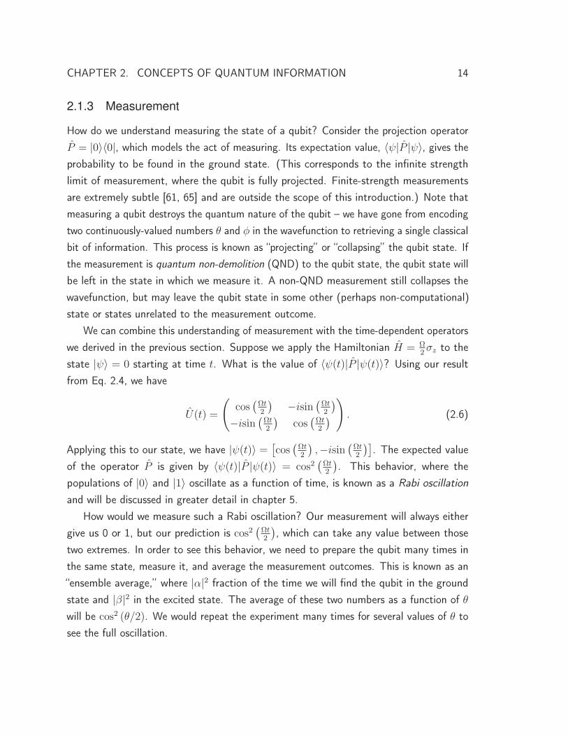
We can combine this understanding of measurement with the time-dependent operatorswe derived in the previous section. Suppose we apply the Hamiltonian H = Ω
2σz to the
state |ψ〉 = 0 starting at time t. What is the value of 〈ψ(t)|P |ψ(t)〉? Using our resultfrom Eq. 2.4, we have
U(t) =
(cos
(Ωt2
) −isin(Ωt2
)−isin
(Ωt2
)cos
(Ωt2
) ) . (2.6)
Applying this to our state, we have |ψ(t)〉 = [cos
(Ωt2
),−isin
(Ωt2
)]. The expected value
of the operator P is given by 〈ψ(t)|P |ψ(t)〉 = cos2(Ωt2
). This behavior, where the
populations of |0〉 and |1〉 oscillate as a function of time, is known as a Rabi oscillationand will be discussed in greater detail in chapter 5.
How would we measure such a Rabi oscillation? Our measurement will always eithergive us 0 or 1, but our prediction is cos2
(Ωt2
), which can take any value between those
two extremes. In order to see this behavior, we need to prepare the qubit many times inthe same state, measure it, and average the measurement outcomes. This is known as an“ensemble average,” where |α|2 fraction of the time we will find the qubit in the groundstate and |β|2 in the excited state. The average of these two numbers as a function of θwill be cos2 (θ/2). We would repeat the experiment many times for several values of θ tosee the full oscillation.
CHAPTER 2. CONCEPTS OF QUANTUM INFORMATION 15
Expectation values
We can also measure the expected value of other projections. For example, the expectedvalue of a Pauli operator given by 〈σj〉 = 〈ψ|σj|ψ〉 indicates the projection of our statevector onto that axis of the Bloch sphere. The projection operator P is related to theexpected value of σz by a constant; the expected value of the other Pauli operators can beunderstood as measuring the qubit along a different axis than the computational basis. Aswe will see in section 2.1.5, the projections of the qubit along each∗ of the Pauli operatorsfully specifies the quantum state.
2.1.4 Multiple qubits
When we have more than one qubit in our system, the number of computational basisstates increases rapidly. The number of states grows exponentially with the number ofqubits N , as 2N . For two qubits, we have four basis states: |00〉, |10〉, |01〉, and |11〉;for three, we have eight states: |000〉, |100〉, |010〉, |001〉, |110〉, |101〉, |011〉, and |111〉,and so on. A quantum state must specify the complex coefficients of all of these basisvectors; this information can no longer be represented as a simple geometrical picture likethe Bloch sphere.
Multi-qubit gates
Gates operating on a manifold of multiple qubits must also be realized. Since the statevector has 2N elements, these operators must be 2N by 2N matrices. Consider a setof k = (i, x, y, z) Pauli operators that each act on only the jth qubit, σj
k, where thesuperscript denotes which qubit it addresses. For example, if we have two qubits, anX-operation on the first qubit would be given by the tensor product of σ1
x and σ2i . A
single-qubit gate is one where all but one of the operators in the tensor product are I;having two or more non-identity operations constitutes a multi-qubit gate. For example, anX-operation on two qubits simultaneously would be given by σ1
X ⊗ σ2X and is commonly
abbreviated as σXX or simply XX.Some particularly common gates include the “SWAP gate,” which maps |01〉 ↔ |10〉
∗ Only three numbers are required; σi tells us nothing because 〈ψ|σi|ψ〉 is defined to be 1 by normalization.
CHAPTER 2. CONCEPTS OF QUANTUM INFORMATION 16
and does nothing to |00〉 or |11〉, and is given by the matrix
SWAP =
⎛⎜⎜⎜⎜⎝1 0 0 0
0 0 1 0
0 1 0 0
0 0 0 1
⎞⎟⎟⎟⎟⎠ . (2.7)
There are also controlled NOT gates, where a target qubit is flipped if and only if a controlis excited, and is given by the matrix
cNOT = Λ(σx) =
⎛⎜⎜⎜⎜⎝1 0 0 0
0 1 0 0
0 0 0 1
0 0 1 0
⎞⎟⎟⎟⎟⎠ . (2.8)
The cNOT is naturally extendible to being “controlled” by more than one qubit; for example,the three-qubit Toffoli gate flips some qubit if and only if two controls are excited, andis therefore also known as a controlled-controlled-NOT or ccNOT gate [66]. Anothercommon two-qubit gate is the controlled phase gate, which flips the phase of only the|11〉 basis state:
cPhase = Λ(σz) =
⎛⎜⎜⎜⎜⎝1 0 0 0
0 1 0 0
0 0 1 0
0 0 0 −1
⎞⎟⎟⎟⎟⎠ . (2.9)
The cPhase also has a multi-qubit generalization known as the Toffoli-sign (or ccPhase)gate which flips the phase of the basis state |1..1〉. Many of these multi-qubit gates can berelated to one another with single-qubit rotations. Experimentally, single-qubit gates areimplemented essentially the same regardless of the number of qubits. Multi-qubit gatesare much more exotic, however. Methods of producing these interactions and using themto entangle qubits will be a major topic of discussion in chapter 7 and chapter 8.
Multi-qubit correlations
Just as there are multiple-qubit gates, we can also define multi-qubit correlations. Single-qubit observables are still defined as the expected value of some tensor-product operatorthat has only one non-identity element. For example, the expected value of X on the first

CHAPTER 2. CONCEPTS OF QUANTUM INFORMATION 17
qubit of a three-qubit register is given by
〈X1〉 = 〈ψ1|〈ψ2|〈ψ3|σ1x ⊗ σ2
i ⊗ σ3i |ψ3〉|ψ2〉|ψ1〉
= 〈ψ1|σ1x|ψ1〉〈ψ2|σ2
i |ψ2〉〈ψ3|σ3i |ψ3〉
= 〈ψ1|σ1x|ψ1〉
(2.10)
where we have used the fact that operators commute through states that do not share thesame labels, and that the states are normalized.
We can also define multi-qubit correlations, where its value is given as the product ofthe two individual correlations. For example 〈Z1Z2〉 tells us the probability that both qubitsare pointing in the same direction along the z-axis. The state |φ+〉 = (|00〉 + |11〉) /√2
would have a 〈Z1Z2〉 value of +1, even though both single-qubit Z correlations are zero.(This is a special state known as a Bell state, see section 2.1.6 below for more.) Note thatthis tells us nothing about which direction either one individually is pointing – merely thatthey are pointing in the same direction. As we will see, the fact that these are independentpieces of information will be crucial both in understanding entanglement and for performingquantum error correction.
Just as with the single-qubit case, knowing all of the expected values of the multi-qubitPauli operators fully specifies a state. With two qubits there are 15 non-trivial correlationsgiven by XI, Y I, ZI, IX, IY , IZ, XX, XY , XZ, Y X, Y Y , Y Z, ZX, ZY , andZZ. Just as you would expect, the number of these linearly-independent correlationsgrows exponentially with the number of qubits, as 4N − 1. Measuring these multi-qubitcorrelations can be done by either post-processing individual but simultaneously performedsingle-qubit measurements, or, as we will see in chapter 7, by exploiting the properties ofmore exotic measurement operators.
2.1.5 The density matrix
The previous sections showed how significantly our state description and operators changewhen we add a single qubit. But what happens if someone snuck in an extra qubit beforewe closed the sample box without us noticing? More generally, how can talk about asubsystem – our group of qubits – when there are so many other degrees of freedomaround? Each atom in our sample box, the helium circulating through our fridge, thebench that our control electronics are sitting on, a plane flying overhead – everything –should, in principle, be included in the wavefunction describing our system. We are forced
CHAPTER 2. CONCEPTS OF QUANTUM INFORMATION 18
to admit that in our experiments, we are only describing and controlling a subset of thesystem, and must therefore come up with a new language to describe it. In particular, thisnew description must contain more information than just an 2N -component vector due tothe fact that our state, viewed as a subset of a larger system, can undergo non-unitaryevolution.∗
We introduce an object called the density matrix defined as
ρ =∑i
pi|ψi〉〈ψi| (2.11)
where |ψi〉 are some complete or over-complete set of states of our subsystem that neednot be orthogonal to one-another and pi ≥ 0 is the probability that the subsystem isin that state, with
∑i pi = 1. (Note that pi is a real-valued probability, and not a
complex probability amplitude.) The expectation value of some operator A is then given by〈A〉 = tr (ρA) =
∑i pi〈ψi|A|ψi〉, where the tr operation is the matrix trace. The density
matrix has three properties worth mentioning right away: it is self-adjoint (e.g. Hermitian)so that ρ = ρ†, it is normalized, so that tr (ρ) = 1, and it is “positive” in the sense that〈ψ|ρ|ψ〉 ≥ 0 for all |ψ〉. The last property further implies that all the eigenvalues of thematrix are greater than or equal to 0.
We define the state purity as tr (ρ2) =∑
i p2i ≤ 1. If it is possible to write the density
matrix with only one non-zero pi, then the purity is 1 and the state can be written as aconventional state vector. For a two-level qubit, the Pauli operators span the space ofHermitian density matrices, so we can write ρ = 1
2(λ0I + λxσx + λyσy + λzσz). Since
tr(ρ) = 1, this simplifies to ρ = 12
(I + �λ · �σ
), with |λ| ≤ 1. The purity of this state
can be shown to be 12
(1 + �λ · �λ
)≤ 1. λj = 〈σj〉 = tr(ρσj), confirming our earlier claim
that by knowing the expected values of all the Pauli operators of a single qubit, we knoweverything that can be known about the state.
We can also introduce a useful property called von Neumann Entropy. It is definedas S(ρ) = −tr [ρlog2ρ] = −∑
j λjlog2(λi). For a pure state like ρ = |0〉〈0|, we haveS(ρ) = 0 and nothing is uncertain; however, for a maximally mixed state like ρ′ =12(|0〉〈0| + |1〉〈1|), S(ρ′) = 1. S has several important properties: for any pure state,
∗ Much of this section and the next are adapted from the lecture notes of Liang Jiang from his Spring 2013course Quantum Information and Computation at Yale University [67].
CHAPTER 2. CONCEPTS OF QUANTUM INFORMATION 19
S(ρ) = 0; S(ρ) ≥ 0 for all ρ; for a system with a d-dimensional Hilbert space, S(ρ) ≤ log2d;and if systems A and B are in some pure state |ψAB〉, S(ρA) = S(ρB).
Density matrix examples
Let us build up some intuition about the density matrix. Suppose the entire universecontains only two qubits, A and B, in some state |ψAB〉, and a thief steals away the B
qubit while we are distracted by something important. What can we say about the stateof A? We can write the total state |ψAB〉 = ∑
i,μ ai,μ|i〉A|μ〉B where |i〉 is a quantumstate of system A and |μ〉 of system B and
∑i,μ |ai,μ|2 = 1. The density matrix of qubit
A is given by the partial trace of the full density matrix, where we sum over the degreesof freedom of B. That is, ρA = trB (ρAB) = trB (|ψAB〉〈ψAB|) =
∑i,j,μ a
∗i,μaj,μ|j〉〈i|,
where again the indices i and j sum over the A states and μ over the B states. Considera specific case where |ψAB〉 = α|00〉 + β|11〉. We have a0,0 = α and a1,1 = β, soρA = |α|2|0〉〈0| + |β|2|1〉〈1| =
(|α|2 0
0 |β|2).
Interestingly, this reduced density matrix cannot be written in terms of a single vector.The state which you might suppose is most similar to it, |ψA′〉 = α|0〉 + β|1〉 has thedensity matrix ρA′ = (α|0〉 + β|1〉) (α∗〈0| + β∗〈1|) = |α|2|0〉〈0|+αβ∗|0〉〈1|+βα∗|1〉〈0|+|β|2|1〉〈1| =
(|α|2 αβ∗
βα∗ |β|2). The astute observer will notice that this is not the same matrix:
the cross-terms that we picked up when expanding |ψ〉〈ψ| give us off-diagonal terms.Those terms indicate the coherences of the state; when we traced away the B qubitabove, those coherences were lost. In the Bloch sphere representation, this is equivalent toforgetting about the φ information while keeping θ. We can calculate the purities of bothcases; for state A′, we find the purity is equal to (|α|2 + |β|2)2 = 1, while for state A wefind a purity of |α|4 + |β|4 ≤ 1. The matrix ρA need not have a vector-state equivalence.
So far, we have introduced the density matrix in the context of a subsystem. However,it also strongly motivated by another experimental reality: the fact that we are alwaysmeasuring an ensemble of prepared states. Suppose that our universe truly contains onlyone qubit, and we are interested in measuring how well we can prepare that qubit insome state. Since quantum mechanics only lets us measure a qubit by projecting it alonga chosen axis, in order to fully characterize the state we must repeatedly prepare andmeasure it many times along several distinct axes, in a similar way that we described tomeasure the Rabi oscillation above. The question then arises: what happens if we donot actually prepare an identical state every time? This might happen if some random
CHAPTER 2. CONCEPTS OF QUANTUM INFORMATION 20
process affects the qubit, such as dephasing or spontaneous emission, if there is noisein our control machinery, if the environment is changing slowly (e.g. the temperatureof the fridge or attenuation of the drive lines), or so on. It turns out that the densitymatrix representation is also equipped to deal with this. An ensemble of imperfect states isdescribed by a density matrix whose purity is reduced as the differences among the statesincreases.
Super-operators
Quantum mechanics predicts that the evolution of the universe, taken as a whole, is unitary.However, when we limit ourselves to a small subset of that system, its interactions withdegrees of freedom outside of our awareness need not be unitary. How must we modifyour operator formalism to model such evolution and ensemble impurity? We introduce anew object called a super-operator which takes a density matrix and maps it to a new one,ρA′ = ε (ρA). ε must obey several properties. First, to be consistent with the propertiesof classical probability, it must be linear, such that ε(λ1ρ1 + λ2ρ2) = λ1ε(ρ1) + λ2ε(ρ2).Second, it must preserve the hermiticity of ρ. Third, it must be trace preserving, so thattr(ρA′) = 1. Fourth, it must be positive, so that 〈ψ|ρA′ |ψ〉 ≥ 0 for all |ψ〉. The Krausrepresentation theorem [68] states that any super-operator ε satisfying these criteria hasan operator representation
ε(ρ) =∑μ
MμρaM†μ (2.12)
for some set of operators Mμ where∑
μ M†μMμ = 1. For a pure state ρ = |ψ〉〈ψ| and a
single operator M0 = O, we see that ε reduces to the normal single-matrix operator weare used to seeing with state vectors. However, if we have more than one Mi, the actionof ε on ρ is no longer unitary and the purity of our state need not be preserved.
This formalism is correct, but quite abstract without a few examples. Let us firstconsider a dephasing channel, where M0 =
√1 − pI, M1 =
√p|0〉〈0|, and M2 =
√p|1〉〈1|.
In some sense, this is a channel where the qubit is randomly measured, which projects awayits phase coherences. The parameter p can be taken to be the probability that the qubithas been dephased. Taking ρ = ( ρ00 ρ10
ρ01 ρ11 ), we calculate ρ′ = ε(ρ) = (1 − p)ρ+ p(ρ00 00 0
)+
p(0 00 ρ11
)=(
ρ00 (1−p)ρ10(1−p)ρ01 ρ11
). If our state ρ = 1
2
(1 + �λ · �σ
), then the new state ρ′ has
λ′ = (λx(1 − p), λy(1 − p), λz). We see that if p = 1, ρ becomes fully dephased and theoff-diagonal terms vanish, just as demonstrated in the above case where our B qubit was
CHAPTER 2. CONCEPTS OF QUANTUM INFORMATION 21
stolen. Note that if the states are separable with |ψ〉 = |A〉 ⊗ |B〉, then there are nocoherences and dephasing (or tracing over B) has no effect on A. It is possible to apply thisprocess continuously using the “Master Equation” partial differential equation formalism.Deriving this equation exceeds the scope of this introduction, but it can be shown that ifdephasing occurs at a rate γ, ρ(t) =
(ρ00(0) ρ10(0)e−γt
ρ01(0)e−γt ρ11(0)
). The dephasing rate γ is often
specified by a characteristic dephasing time T2 = 1/γ.Another relevant example is the amplitude damping channel ∗. There, M0 =
(1 00√1−p
)and M1 =
(0√p
0 0
)=
√p|0〉〈1|. Repeating the calculation above, we find that λ →
λ′ =(√
1 − pλx,√1 − pλy, p+ (1 − p)λz
). Again, if we were to apply this operation
continuously, we can define its rate γ to be equal to 1/T1, where T1 is the characteristictime of the qubit for it to relax from |1〉 back to |0〉. The maximum T2 is given by 2T1.Interestingly, this decay channel’s eigenstate is not a maximally mixed state, but rather theground state |0〉〈0|. Finally, the third common process is the depolarizing channel. There,M0 =
√1 − pI, M1 =
√p3σx, M2 =
√p3σy, and M3 =
√p3σz. This is often considered
the most severe damage that you can inflict on a qubit state, since λ → λ′ =(1 − 4p
3
)λ,
making the qubit completely impure (e.g. |λ′| = 0) for p = 3/4. In the context of quantumerror correction, undoing a depolarizing error is the most demanding task for a code.
2.1.6 Entanglement
The phenomenon of quantum entanglement is one of the most famous and “spooky”predictions of quantum theory. It refers to the fact that the quantum state of one particlecan depend on the state of another. For example, take the Bell state mentioned abovewhere |φ+〉 = (|00〉 + |11〉) /√2. Measured individually, both qubits are equally likelyto point in either direction along the z-axis, but if one qubit is found to be pointingup then the other will as well, and vice versa. That is, their behaviors are random butcorrelated. An entangled state is one where the state |ψAB〉 cannot be written as a
∗ M0 accounts for the possibility that the channel did not cause the qubit to decay. Why, then, does M0 �= I?Suppose we are performing an experiment where we are measuring the qubit with a photodetector, whichclicks when the qubit decays and emits a photon. As we wait and are attempting to infer the state of thequbit, the longer our photodetector does not click, the more we have to account for the possibility thatthe qubit was not in its excited state to begin with. Similarly, if we fail to detect photons leaking outof a cavity supposedly containing some large coherent state, we must consider the possibility that thecavity actually contains a smaller state that which is less likely to have emitted a photon. Thus, the M0
operator reduces our estimate of the excited state population. This phenomenon is known as the “dogthat did not bark”; if our guard dog is silent, it may be that there are no robbers trying to break in, but italso might be that the dog is simply absent (or asleep).
CHAPTER 2. CONCEPTS OF QUANTUM INFORMATION 22
separable state, the product of two wave functions individually spanning the constituentsubsystems, |ψA〉⊗|ψB〉. Quantifying entanglement requires defining what your subsystemsare. Mathematically, entanglement is a consequence of the fact that each coefficientof a multi-component wavefunction is independent. Viewed from the point of view ofelements in a vector, there is no discrimination between subsystems – no inherent meaningof the basis vectors. It is only in the context of delineations between subsystems thatentanglement is meaningful. For example, an atom with four energy levels and two two-levelqubits would have the same Hilbert space, but we would only say that the two separateatoms could meaningfully be entangled.
More formally, we define the Schmidt decomposition for two systems A and B as
|ψAB〉 =∑j
√λj|Uj〉A|Vj〉B (2.13)
where∑
j λj = 1 and the states |U〉A, |V 〉B form a complete orthonormal basis for thesystems A and B, respectively. Any pure state can be written in this form∗. If it is notpossible to find a basis in which we can write |ψAB〉 using only one non-zero λj , then thestate is entangled. For pure states, we can also say that if the von Neumann entropy ofsome subsystem is greater than zero, it is entangled with some other subsystem. If thevon Neumann entropy is maximal, the state is also maximally entangled. Interestingly,since the entropy of the full pure state is zero but the entropy of the subsystems are not,there seems to be some “negative entropy” associated with entanglement.
Generating entangled states
How is entanglement generated? We know immediately that any local operation cannotchange the amount of entanglement. A local operation is one which leaves invariantthe basis vectors of a subsystem that it does not address. Consider the HamiltonianH = HA + HB where HA leaves invariant system B and vice versa, and [HA, HB] = 0.The unitary evolution driven by this Hamiltonian is also separable, since U = e−iHt =
e−i(HAt+HBt) = e−iHAte−iHBt = UAUB when their commutator is zero. If we start with anunentangled state |ψAB〉 = |ψA〉 ⊗ |ψB〉, applying this unitary to the state also gives usan unentangled state, since U |ψAB〉 = UA|ψA〉UB|ψB〉 = (UA|ψA〉) ⊗ (UB|ψB〉), whichis still separable. Moreover, if we have an entangled state, this local operation will only
∗ The proof can be found in Nielsen and Chuang [68] on page 109.
CHAPTER 2. CONCEPTS OF QUANTUM INFORMATION 23
change the vectors in the Schmidt decomposition and not the number or magnitude ofthe λi’s, leaving the amount of entanglement unchanged.
Generating entanglement therefore must involve non-local operations which do notcommute with the any of the subsystems we are attempting to entangle. We can seethis with an example. Suppose H = gσA
x ⊗ σBx , which gives U = e−iHt = cos(gt)I −
isin(gt)σAx ⊗ σB
x . Applying this to the state |00〉 for t = π4g
gives us 1√2(|00〉 − i|11〉),
which is a maximally-entangled two-qubit state with S(ρA) = S(ρB) = 1 and S(ρAB) = 0.Another Hamiltonian that will be useful later is given by H = g
(1−σA
z
2
)(1−σB
z
2
). This
operation, which contains all the Pauli Z operators σZI , σIZ , and σZZ , maps to theunitary U = diag{1, 1, 1,−1} at t = π/g, which we identify as a controlled-phase gate –it flips only the phase of the basis state |11〉. We can also make a controlled-NOT gate,which flips the state of qubit B if and only if qubit A is excited using the HamiltonianH = g
(1−σA
z
2
)(1−σB
x
2
).
There are certain classes of entanglement that are particularly famous. For twoqubits, we have already mentioned the Bell state |φ+〉 = |00〉+|11〉√
2. We can also construct
a Bell basis with the addition of the states |φ−〉 = |00〉−|11〉√2
, |ψ+〉 = |01〉+|10〉√2
, and|ψ−〉 = |01〉−|10〉√
2. Each of these states is maximally entangled, mutually orthogonal, and
span the two-qubit Hilbert space. We can write product states in this basis since it
is complete, for example |00〉 =|φ+〉+|φ−〉√
2. For three qubits, there are two separate
classes of entanglement: GHZ and W-type states [69]. The canonical GHZ (Greenberger-Horne-Zeilinger) state [70] is given by |GHZ〉 = (|000〉 + |111〉) /√2 and the W stateby |W 〉 = (|100〉 + |010〉 + |001〉) /√3. These two states are not transformable to oneanother with local operations, so we can say that each of these entanglement classes forma manifold of states. For example, the state |GHZ ′〉 = (|010〉 + |101〉) /√2 still counts asa GHZ-class state since it is modified from its prototype by an X-operation on the secondqubit, and no application of single-qubit rotations could change it into a W state. Asthe number of qubits increases, so too does the number of distinct entanglement classes;GHZ and W types generalize to more qubits in an obvious way, but the additional classesare very complicated and constitute an active research question [71].
Entanglement of impure states
The method of detecting entanglement we mentioned earlier does not work if the stateunder test is impure: states no longer have a defined Schmidt decomposition and their
CHAPTER 2. CONCEPTS OF QUANTUM INFORMATION 24
purity can be less than 1 without entanglement. However, we can extend our languageto deal with these states as well. We previously defined a separable state as one thatcan be written as |ψAB〉 = |ψA〉 ⊗ |ψB〉. When talking about a density matrix, we candistinguish between two types of unentangled states: an uncorrelated state and a separablestate. An uncorrelated state can be written as ρun = ρA ⊗ ρB, while a separable stateas ρsep =
∑k pkρ
kA ⊗ ρkB, with
∑k pk = 1 and pk ≥ 0. That is, a separable state is an
incoherent sum of uncorrelated states. If our density matrix cannot be written in eitherof these forms, we can say it is entangled. Rigorously distinguishing the presence ofentanglement with impure states is outside the scope of this introduction. However, atleast for two qubits, the “positive partial transpose” (PPT) is definitive [72, 73].
2.2 Computing with qubits
Why are qubits potentially useful for computing? Broadly speaking, quantum informationscience seeks to take advantage of two properties of quantum mechanics: superpositionand parallelism. We have already seen that the amount of information stored in a singlequbit is in some sense much greater than a single bit, with its state described by tworeal numbers. This fact is compounded when describing the wavefunction of a system ofseveral qubits: for two qubits, there are six real numbers, with three there are fourteen,and so on. For N qubits, there are 2(2N − 1) real numbers that describe a pure quantumstate (and more, 2N+1 − 1, if the state is impure, though this information is not necessarilyuseful); for N = 200, this is more real numbers than there are atoms in the universe. Evena relatively small number of qubits (by the standard of modern computers), stores anincredible density of information. Moreover, if we had some unitary that acts on thesequbits, it would operate on all the basis states simultaneously. That is, for some unitaryU , |00..0〉 → U |00..0〉, |10..0〉 → U |10..0〉, and so on through |11..1〉 → U |11..1〉. Evenif our qubit is in some vast superposition of states, a unitary operation acts on eachconstituent equally rapidly. Not only can we store a huge amount of information in aregister of qubits, then, but we can also manipulate that information very efficiently aswell.
Unfortunately, things are not as favorable as these facts might imply due to the realitiesof quantum measurement. As we saw in the previous section, a measurement can onlyreturn the value of one observable. When a qubit is in an eigenstate of that observable(e.g. it is already pointing along the direction you are measuring), the measurement will
CHAPTER 2. CONCEPTS OF QUANTUM INFORMATION 25
not destroy any information since the qubit is merely projected to itself. However, inany other case it will randomly project the qubit along one of the possible eigenstates.Thus, the best you can do to extract the expected value of some observable is to prepareand measure the state many times in succession. There is also no way of isolating ormeasuring a single coefficient of one basis vector without many repetitions; you cannottell if a coefficient is identically zero, for example, or simply very small. Thus, it seemsthat this huge amount of information stored and manipulated in our quantum state is notuseful to us because we cannot efficiently retrieve it.
2.2.1 Quantum algorithms
Thankfully, the problem of measurement is surmountable because of quantum interference.Using it, the answer to a simple (e.g. yes-or-no) question might be encoded in an observableor observables that can be extracted efficiently. For example, the quantum amplitude ofa basis state corresponding to the correct answer might be amplified at the cost of anincorrect state’s population. A quantum algorithm would take advantage of the qualities ofquantum mechanics to solve certain problems faster than is possible classically. However,because of the difficulty of getting around the issue of measurement, only a few usefulquantum algorithms have so far been discovered [74, 75]. The most well-known examplesinclude Grover’s search algorithm, which can search an unstructured database quadraticallyfaster than is possible with a classical computer [76, 77], Shor’s factoring algorithm, whichis exponentially faster than is believed to be possible classically [14], and the Deutsch-Jozsaalgorithm for determining whether a function is balanced or constant, which also grants anexponential increase [13], though many more exist [78]. The first two algorithms will onlyreturn a correct answer with a high probability and may require several repetitions (thoughit is efficient to check if they succeeded). This is in contrast to Deutsch-Jozsa, which isdeterministic and will always return the correct value if the algorithm was run successfully.The details of how these algorithms work will not be covered here, but often take advantageof more fundamental quantum subroutines like phase estimation, the quantum discreteFourier transform, and basis state amplitude amplification [75].
2.2.2 DiVincenzo criteria
Just as classical algorithms do not require a particular type of computer as long as theyimplement certain functionality, quantum algorithms are also agnostic about their physical

CHAPTER 2. CONCEPTS OF QUANTUM INFORMATION 26
implementation. Any quantum computer must satisfy certain requirements, however, whichwere first enumerated by David P. DiVincenzo and are known as the DiVincenzo criteria[79]. This section will briefly introduce and explain each of these and several additionalrequirements for error correction.
1) “A scalable physical system with well characterized qubits”
A quantum computer must be made up of many quantum bits, which both exhibit quantumproperties (superposition and entanglement) and can be produced in large quantities. Theymust be “well characterized,” in the sense that their physical parameters are accuratelyknown (for example, the energies of states) as well as their couplings to other qubits andthe environment. The Hamiltonian of the qubit itself must be understood, so that, e.g. ifthere are higher excited states of the bit we can ensure that qubit population is containedto the computational Hilbert space.
2) “The ability to initialize the state of the qubits to a simple fiducial state,such as the ground state”
We must be able to initialize the computer in some state |ψ〉 = |00...〉 for two reasons.First, any algorithm would require the computational register to be in some known state tobegin a computation, since its evolution is unitary and “garbage in” would map to “garbageout.” Second, as we will see, it is necessary to perform error correction on any quantumcomputer, which requires a steady stream of qubits in some pure state to extract entropy.For that reason, this requirement might be expanded to not only include the initializationof the computer in some known state, but also the real-time preparation of extra “ancilla”qubits in a known state during computation.
3) “Long relevant decoherence times, much longer than the gate operationtime”
In order to successfully run an algorithm, a quantum computer must accurately storethe information it is working on. As discussed above in section 2.1.5, any corruption ofinformation is known as decoherence, and can be understood as the unintentional couplingto the environment, noise in control signals, and so on. The time it takes to do any partof an algorithm must be much faster than the characteristic time of this information loss.

CHAPTER 2. CONCEPTS OF QUANTUM INFORMATION 27
Note that the total algorithm run time need not be short compared to the decoherencetime because of the existence of quantum error correction. As long as errors can be quicklyidentified – that is, as long as the error rate for a given operation is below some threshold– some amount of decoherence is tolerable.
4) “A ‘universal’ set of quantum gates”
Any quantum algorithm is a set of deterministic unitary instructions that involve somenumber of qubits. For example, an algorithm might call for a unitary U1 to be applied,followed by another unitary U2, and so on. Then, to run that algorithm, we would turn onsome Hamiltonian H1 for some time, followed by H2, and so on. In practice, it is verychallenging to implement a series of arbitrary Hamiltonians. It is more convenient to breakthem down into some set of constituent parts like we did with the Pauli operators forsingle-qubit rotations. Just as with a classical computer, where having the NAND gateis sufficient to do any fundamental logic operation (NOT, AND, OR, NOR, XOR, andXNOR operations all have simple circuit diagrams involving only NANDs), many quantumoperations can be comprised from the others. For example, a controlled-phase gate can beturned into a controlled-NOT with the addition of Hadamard gates on the target qubitbefore and after [68]. Thus, there are many possible sets of “universal” gates. One set ofgates that can be shown to be universal is the combination of the Hadamard, a Z rotationby π/4 (mysteriously known as the π/8 gate), and the controlled-NOT gate. Having suchtenuous control is not ideal; it increases the overhead to construct whatever unitary wemight need. More control, like arbitrary rotations of single qubits or additional two orthree-qubit gates, is better.
5) “A qubit-specific measurement capability”
We will need to extract information from our computer to retrieve its results, and sosome sort of measurement mechanism is required. The words “qubit-specific” are slightlymore controversial, however. A measurement of some group property of qubits, like theirprojection onto a specific basis state, is insufficient. While an algorithm could possibly betailor-made for a different measurement operator, individual qubit measurement is crucialfor extracting error syndromes to perform quantum error correction [80]. Also, if a singlemeasurement is not reliable enough, with the ability to measure qubits individually, youcould potentially perform controlled-NOT gates between the qubit and several ancillae and
CHAPTER 2. CONCEPTS OF QUANTUM INFORMATION 28
then measure those and tabulate the results to improve the fidelity. For example, we couldmap (α|0〉 + β|1〉) ⊗ |0000〉 → α|00000〉 + β|11111〉 using entangling gates and then doa majority-rules vote on the measurement result of all those qubits.
Requirements for fault tolerance
There are also specific requirements for fault tolerant quantum error correction [20] (asdefined and discussed in section 2.3.6), in addition to the well-known error threshold. Wemust be able to perform operations on many qubits in parallel, so that we can keep up aswe grow the computer and increase the error channels. Since most physical “qubits” areactually larger quantum systems and error correction only addresses the computationalHilbert space, we must be able to ensure that we do not leave that space, or at least havea means of unconditionally pumping population back to it. We need a continuous sourceof initialized qubits to absorb entropy; it is not enough to simply initialize all the qubitsat the beginning of the algorithm because their purity will drop exponentially as timegoes on. And finally, we require that errors do not scale unfavorably with the size of thecomputer (e.g. the error rate per qubit does not depend on the size) and that the errorsare not strongly correlated between qubits (e.g. many qubits cannot fail simultaneously, orthe code will be overwhelmed, as we explain in section 2.3.4). As a corollary to this, thearchitecture used to couple qubits together must not cause errors to propagate betweenqubits [80].
Additional “desiderata”
The five enumerated requirements are necessary to do computation. There are, however,several other abilities that would be extremely desirable from a practical point of view[81]. The ability to both convert a stationary quantum bit into a “flying” qubit like aphoton and then transmit it large distances is crucial for quantum-enabled communication[82, 83]. Access to gates between physically distant qubits can reduce the requirementson error thresholds by one or two orders of magnitude compared to being limited to onlynearest-neighbor cNOTs [84, 85]. Fast and reliable measurement and classical computation,so that we can take advantage of the extremely low error rates of classical computers toimplement our error correction, also dramatically reduces overhead [86]. (In principle, aquantum computer can implement the classical logic that would follow a measurement, butsince the error rates of quantum gates are much higher and we do not require quantumness
CHAPTER 2. CONCEPTS OF QUANTUM INFORMATION 29
to perform these corrections, it is preferable to use a classical computer.) Some amountof error correlation is tolerable, but the less the better, as is a high degree of parallelismand a large supply of extra ancilla qubits. Finally, exceeding the error threshold by alarge amount also reduces the overhead required by a code; in practice, we would want toexceed it by two or more orders of magnitude so that the number of qubits required is notexcessive [80].
2.3 Quantum errors and error correction
As we have seen in the previous section, because continuous unitary evolution can occuron a vast multitude of simultaneous basis states, a quantum computer is potentially muchmore powerful than a classical one. However, that same property also makes it intrinsicallymore sensitive to errors. Quantum algorithms like the quantum discrete Fourier transformoften rely on maintaining minute phase differences between states; any source of noise orcontrol error may corrupt these continuous-valued parameters and cause the computationto fail. Moreover, because evolution is continuous, even tiny errors will inexorably build upas time goes on, foiling our computational aspirations or at least limiting them to trivialproblems.
This section will introduce the concept of quantum error correction, which can the-oretically save us from this predicament. We start by clarifying the difference betweena classical and quantum error and will introduce a simple classical error correcting code.We will then argue that there are three major reasons that we might expect this errorcorrecting code should fail in the quantum case. However, by being clever enough, we canbypass each issue and propose a quantum bit-flip code. This code, which requires onlythree qubits to operate, does not correct for all possible errors but represents a prototypefor more sophisticated quantum codes. We will explain this code in detail and demonstratethat, with a small modification, it can correct for phase errors instead. We will end byintroducing other quantum codes which can correct for arbitrary errors and discuss therequirements for fault tolerance.
2.3.1 Classical vs. quantum errors
Let us begin by discussing the reasons why a classical computer typically does not requireerror correction during normal operation. Consider the state of a classical switch (e.g. a
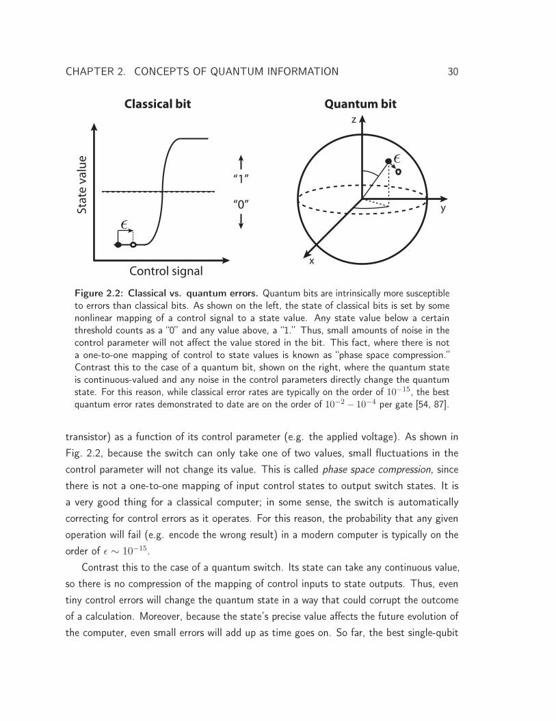
CHAPTER 2. CONCEPTS OF QUANTUM INFORMATION 30
z
y
x
ε
Quantum bitClassical bit
Control signal
Stat
e va
lue
“1”
“0”
ε
Figure 2.2: Classical vs. quantum errors. Quantum bits are intrinsically more susceptibleto errors than classical bits. As shown on the left, the state of classical bits is set by somenonlinear mapping of a control signal to a state value. Any state value below a certainthreshold counts as a “0” and any value above, a “1.” Thus, small amounts of noise in thecontrol parameter will not affect the value stored in the bit. This fact, where there is nota one-to-one mapping of control to state values is known as “phase space compression.”Contrast this to the case of a quantum bit, shown on the right, where the quantum stateis continuous-valued and any noise in the control parameters directly change the quantumstate. For this reason, while classical error rates are typically on the order of 10−15, the bestquantum error rates demonstrated to date are on the order of 10−2 − 10−4 per gate [54, 87].
transistor) as a function of its control parameter (e.g. the applied voltage). As shown inFig. 2.2, because the switch can only take one of two values, small fluctuations in thecontrol parameter will not change its value. This is called phase space compression, sincethere is not a one-to-one mapping of input control states to output switch states. It isa very good thing for a classical computer; in some sense, the switch is automaticallycorrecting for control errors as it operates. For this reason, the probability that any givenoperation will fail (e.g. encode the wrong result) in a modern computer is typically on theorder of ε ∼ 10−15.
Contrast this to the case of a quantum switch. Its state can take any continuous value,so there is no compression of the mapping of control inputs to state outputs. Thus, eventiny control errors will change the quantum state in a way that could corrupt the outcomeof a calculation. Moreover, because the state’s precise value affects the future evolution ofthe computer, even small errors will add up as time goes on. So far, the best single-qubit
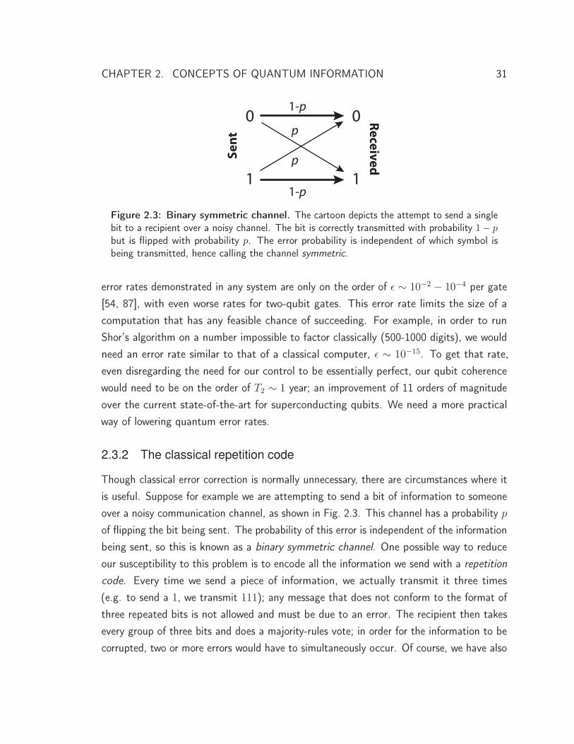
CHAPTER 2. CONCEPTS OF QUANTUM INFORMATION 31
Se
nt
Re
ceiv
ed
0
1
0
11-p
1-p
p
p
Figure 2.3: Binary symmetric channel. The cartoon depicts the attempt to send a singlebit to a recipient over a noisy channel. The bit is correctly transmitted with probability 1− pbut is flipped with probability p. The error probability is independent of which symbol isbeing transmitted, hence calling the channel symmetric.
error rates demonstrated in any system are only on the order of ε ∼ 10−2 − 10−4 per gate[54, 87], with even worse rates for two-qubit gates. This error rate limits the size of acomputation that has any feasible chance of succeeding. For example, in order to runShor’s algorithm on a number impossible to factor classically (500-1000 digits), we wouldneed an error rate similar to that of a classical computer, ε ∼ 10−15. To get that rate,even disregarding the need for our control to be essentially perfect, our qubit coherencewould need to be on the order of T2 ∼ 1 year; an improvement of 11 orders of magnitudeover the current state-of-the-art for superconducting qubits. We need a more practicalway of lowering quantum error rates.
2.3.2 The classical repetition code
Though classical error correction is normally unnecessary, there are circumstances where itis useful. Suppose for example we are attempting to send a bit of information to someoneover a noisy communication channel, as shown in Fig. 2.3. This channel has a probability p
of flipping the bit being sent. The probability of this error is independent of the informationbeing sent, so this is known as a binary symmetric channel. One possible way to reduceour susceptibility to this problem is to encode all the information we send with a repetitioncode. Every time we send a piece of information, we actually transmit it three times(e.g. to send a 1, we transmit 111); any message that does not conform to the format ofthree repeated bits is not allowed and must be due to an error. The recipient then takesevery group of three bits and does a majority-rules vote; in order for the information to becorrupted, two or more errors would have to simultaneously occur. Of course, we have also

CHAPTER 2. CONCEPTS OF QUANTUM INFORMATION 32
gone from having one faulty bit to having three, so the likelihood of an error occurring hassubstantially increased. The probability Pn of having n bit-flips is given by P0 = (1 − p)3,P1 = 3p(1 − p)2, P2 = 3p2(1 − p) and P3 = p3. Thus, the probability for the code tofail is given by peff = P2 + P3 = 3p2 − 2p3. Crucially, this error rate no longer has anylinear dependence on p; for p < 1/2, the effective error rate is less than p and adding theredundancy of the extra faulty qubits benefits rather than detracts. The smaller the valueof p, the greater the improvement due to performing this code; for example, if p = 10−4,peff = 3 · 10−8. Moreover, if we require a higher-order reduction we can employ greateramounts of redundancy (e.g. sending 5 or 7 bits for every 1 we wish to transmit).
2.3.3 The challenges of quantum errors
Implementing such a repetition code with quantum bits seems like it might help ourproblem. While we do not necessarily need to transmit a quantum state over a noisychannel to perform quantum computation (though this would be required for things likequantum key distribution), we could think of the “channel” as simply the passage of time.That is, as we let our qubit sit in some state, it will inevitably interact with the environmentand decohere, causing an error. Can we implement the repetition code with quantum bits?There are actually three good reasons to think the answer is no, which initially seemed toindicate that quantum error correction was impossible [68]. First, the no-cloning theoremprohibits the copying of quantum states [7]. Second, measuring the states to see if theyare the same does not seem to help us detect the presence of an error and will necessarilydestroy their quantum information. And third, we must correct for continuous rather thandiscrete errors and so might expect to need an infinite amount of redundancy to distinguisheach possible error. Let us investigate each one of these and introduce why they present aproblem.
The no-cloning theorem
The no-cloning theorem states that it is impossible to create an identical copy of a quantumstate. It is surprisingly easy to prove [7]. Suppose we have a qubit A that is in some state|ψ〉A that we want to copy and a qubit B in some initial state |i〉B. If we have the ability toclone our state, there must be some unitary such that U |φ〉A|i〉B = |φ〉A|φ〉B. U preservesthe inner product, so 〈i|B〈φ|A|ψ〉A|i〉B = 〈i|B〈φ|AU †U |ψ〉A|i〉B = 〈φ|B〈φ|A|ψ〉A|ψ〉B,where we have introduced the state |φ〉A which is some arbitrary state of A. Since
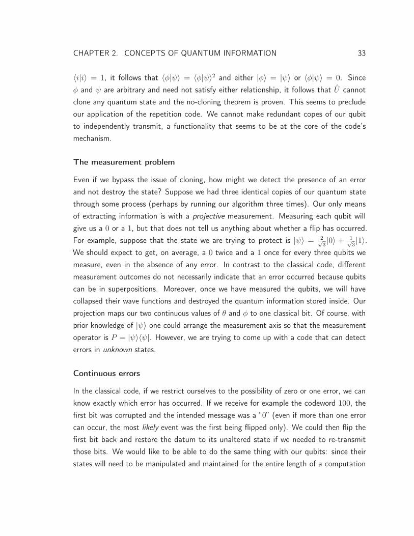
CHAPTER 2. CONCEPTS OF QUANTUM INFORMATION 33
〈i|i〉 = 1, it follows that 〈φ|ψ〉 = 〈φ|ψ〉2 and either |φ〉 = |ψ〉 or 〈φ|ψ〉 = 0. Sinceφ and ψ are arbitrary and need not satisfy either relationship, it follows that U cannotclone any quantum state and the no-cloning theorem is proven. This seems to precludeour application of the repetition code. We cannot make redundant copes of our qubitto independently transmit, a functionality that seems to be at the core of the code’smechanism.
The measurement problem
Even if we bypass the issue of cloning, how might we detect the presence of an errorand not destroy the state? Suppose we had three identical copies of our quantum statethrough some process (perhaps by running our algorithm three times). Our only meansof extracting information is with a projective measurement. Measuring each qubit willgive us a 0 or a 1, but that does not tell us anything about whether a flip has occurred.For example, suppose that the state we are trying to protect is |ψ〉 = 2√
3|0〉 + 1√
3|1〉.
We should expect to get, on average, a 0 twice and a 1 once for every three qubits wemeasure, even in the absence of any error. In contrast to the classical code, differentmeasurement outcomes do not necessarily indicate that an error occurred because qubitscan be in superpositions. Moreover, once we have measured the qubits, we will havecollapsed their wave functions and destroyed the quantum information stored inside. Ourprojection maps our two continuous values of θ and φ to one classical bit. Of course, withprior knowledge of |ψ〉 one could arrange the measurement axis so that the measurementoperator is P = |ψ〉〈ψ|. However, we are trying to come up with a code that can detecterrors in unknown states.
Continuous errors
In the classical code, if we restrict ourselves to the possibility of zero or one error, we canknow exactly which error has occurred. If we receive for example the codeword 100, thefirst bit was corrupted and the intended message was a “0” (even if more than one errorcan occur, the most likely event was the first being flipped only). We could then flip thefirst bit back and restore the datum to its unaltered state if we needed to re-transmitthose bits. We would like to be able to do the same thing with our qubits: since theirstates will need to be manipulated and maintained for the entire length of a computation
CHAPTER 2. CONCEPTS OF QUANTUM INFORMATION 34
(which may take months), we must periodically refresh their state by applying the inverseof the error that has occurred∗.
For quantum errors, this seems to pose a daunting challenge. We started this sectionby arguing that qubits were especially sensitive to errors exactly because there are so manyways that things can go wrong. While a classical bit can undergo only one discrete error –being flipped – a qubit could undergo any spurious evolution in two continuous dimensions.If we need to correct a qubit to some high precision, it would seem that we would needto know the precise unitary that caused the error to equal precision. And because thereare in some sense an infinite number of different errors, does that imply that we need aninfinite set of resources to distinguish each one?
2.3.4 The quantum repetition code
Somewhat miraculously, none of these issues are prohibitive. There is a simple quantumcode that can correct for arbitrary bit-rotations of a qubit. To explain it, we first notethat the bit-flip code we described actually uses more information than is necessary tofix an error. We do not need to know the value of the bits being sent, we only need toknow whether they are the same as the other bits. For example, whether our code word is101 or 010 does not change the identification of the error – the middle bit was flipped inboth cases. In the language we have developed, we need not know 〈Z〉 for each qubit,but rather 〈ZZ〉 for both pairs. This key observation turns out to save us from all threeproblems previously identified.
The quantum repetition code encodes a single qubit on a manifold of three qubits, asdoes its classical analog. What is this encoding? We already know that we cannot copy ourstate three times because of the no-cloning theorem, but we can do something even betterusing entanglement. We map (α|0〉1 + β|1〉1)|0〉2|0〉3 → α|000〉 + β|111〉, where the firstqubit stores some state we would like to protect, the second and third qubits are known asancillas and are initialized in the ground state, and the notation |abc〉 refers to the stateof the first, second, and third qubit respectively. This state, where the three qubits areall in the same state as one another but individually are pointing in no definite direction,is a three-qubit entangled state known as a “GHZ-like” state. When |α| = |β| = 1√
2it
∗ In some codes, simply keeping track of exactly which error has occurred to each qubit and incorporatingthat knowledge into future operations or in interpreting the final result is enough. You do not necessarilyhave to correct the error in-situ, but you do have to know exactly what happened.

CHAPTER 2. CONCEPTS OF QUANTUM INFORMATION 35
is maximally entangled and the state is a GHZ state without qualification, as defined insection 2.1.6.
The unitary responsible for mapping α|0〉+ β|1〉 to this state is two controlled-NOTgates between qubits 1 and 2 and 1 and 3, U = N2
1N31 . The operation of a single
controlled-NOT flips the target qubit if and only if the control qubit is excited. Becausethe operation is coherent, it will act on only the subspace where this is true. Thus,N2
1 (α|0〉1+β|1〉1)|0〉2 = α|00〉+β|11〉 and the extension to three qubits is obvious. Notethat the state is not being copied; if any one of the qubits were measured, the entire statewould be projected. Interestingly, this kind of state is actually more susceptible to noisebecause if any single one of the qubits is dephased, all three states are lost. For the samereason, an entangled state may be interesting for applications to sensing or detection sinceits sensitivity to fields that affect all the qubits grows like N instead of
√N , as found
classically∗.
GHZ-like states
These states have the valuable property that they are simultaneous eigenstates of thethree Pauli ZZ operators. For example, Z1Z2|φ0〉 = Z1Z2α|000〉 + Z1Z2β|111〉 =
(+1)(+1)α|000〉 + (−1)(−1)β|111〉 = α|000〉 + β|111〉, so the state |φ0〉 has eigenvalue+1 for the operator Z1Z2 (and also for Z1Z3 and Z2Z3, though knowing any two ofthese correlations implies you know the third; we omit Z1Z3 henceforth). Somethingvery interesting happens if we suppose that one of the qubits was flipped, so we have|φ1〉 = α|100〉 + β|011〉. We calculate that Z1Z2 now equals −1 (and Z2Z3 = +1). Thesign of the eigenvalue has changed in response to the error. We list the eigenvalues for allfour possible cases – either no error or a bit-flip of exactly one of the three qubits – intable 2.1. Luckily, each of these errors has a distinct set of values of the ZZ eigenvalue –a unique error syndrome. Moreover, we can in principle measure these error syndromeswithout learning anything about the encoded state – these syndromes are independent ofthe values of α and β. We have thus made a huge amount of progress. Not only have wecome up with an encoding that does not violate the no-cloning theorem, but there are a
∗ Affecting all the qubits equally would correspond to correlated noise, which would diminish our ability tocorrect errors. For example, if the noise channel never caused a single flip but instead always flipped twobits at a time, the code we have described would fail. A similar pattern holds true with quantum codes;correlations in noise that make double errors more likely than they would otherwise be must be limited orat least well-understood if we hope to build a quantum computer.
CHAPTER 2. CONCEPTS OF QUANTUM INFORMATION 36
State Error Z1Z2 Z2Z3
|φ0〉 = α|000〉 + β|111〉 None +1 +1|φ1〉 = α|100〉 + β|011〉 Q1 −1 +1|φ2〉 = α|010〉 + β|101〉 Q2 −1 −1|φ3〉 = α|001〉 + β|110〉 Q3 +1 −1
Table 2.1: Eigenvalues of the GHZ states. Each of the four error syndromes has a uniquesignature in the values of Z1Z2 and Z2Z3 which can be determined without knowledge of αor β. This fact is the basis of the quantum repetition code.
set of observables∗ that unambiguously identify which error has occurred on that state(assuming that there was at most one error). We have thus gotten around two of thethree major problems we had identified with correcting quantum errors. We see how tocircumvent the third problem in the next section.
Measurement-based quantum repetition code
We saw in the last section that if we know the values of both ZZ eigenvalues of ourGHZ-like state, we can unambiguously detect the presence of a single bit-flip. But whathappens if a finite rotation (that is, a superposition of a bit-flip and no bit-flip) occurs? Itturns out that this is also correctable by the three-qubit quantum repetition code. To seethis, we need to be specific about how the code works. The code is shown as a “quantumcircuit” in Fig. 2.4, where each horizontal line represents the action on a single qubit asa function of “time.” The code begins with the situation that we have a qubit in somestate that we wish to protect, |ψ〉 = α|0〉 + β|1〉, here the second qubit, and two “ancilla”qubits – one and three – in their ground state. As described above, the circuit that mapsthis state α|0〉 + β|1〉 → α|000〉 + β|111〉 consists of two controlled-NOT gates, depictedby black dots and crossed, open circles connected by a line. The qubit that has the opencircle is flipped if and only if the qubit with the black dot is excited. After these two gates,the three-qubit manifold is in the encoded GHZ-like state. Suppose now that one of the
∗ The operators Z1Z2 and Z2Z3 are known as stabilizer operators, following the formalism of DanielGottesman [88]. They have the property that they commute both with one another and that our GHZ-likestate is an eigenstate of them both. Our manifold of three qubits is reduced to a single-qubit degreeof freedom with the constraint that the three-qubit state must be an eigenstate with eigenvalue +1 forboth operations. The stabilizer operators also commute with the “logical qubit operators” Xl = X1X2X3,Yl = iXlZl, and Zl = Z1Z2Z3 which perform rotations on the encoded qubit α|0〉l + β|1〉l, where|0〉l = |000〉 and |1〉l = |111〉.

CHAPTER 2. CONCEPTS OF QUANTUM INFORMATION 37
|0〉 ��� X |0〉α|0〉 + β|1〉 • • E • • X α|0〉 + β|1〉
|0〉 ��� X |0〉
LogicZ2Z3
Z1Z2
encode error diagonise fix
α|000〉 + β|111〉
|α| = |β|GHZ state for
|Z1Z2 Z2Z3〉α|111〉 + β|101〉
α|010〉 + β|101〉
= (α|1〉 + β|0〉) ⊗ |11〉
Figure 2.4: Measurement-based QEC circuit. The code begins by mapping a single-qubitstate α|0〉 + β|1〉 to the three-qubit entangled state α|000〉 + β|111〉. A single bit-flip isshown on the middle qubit, making the state α|010〉+β|101〉. The encoding is then reversed,leaving the middle qubit in a quantum state, related to its original state possibly by an errorrotation, and the ancilla qubits with the values of the error syndromes. These qubits are thenmeasured and the results processed with classical logic, which triggers conditional rotationsthat return the quantum register to its original state. Small error rotations are projected tofull flips or nothing by the measurement process. This quantum code corrects for a singleerroneous rotation of any qubit.
qubits is fully flipped; for concreteness, say the second qubit, so the manifold will now bein the state α|010〉 + β|101〉.
At this point, we wish to detect the presence of an error. We do this by reversing theencoding step with two more controlled-NOT gates∗. For our case of the second qubitbeing flipped, the qubits will now be in the state (α|1〉 + β|0〉)⊗ |11〉, where we have firstlisted the state of the second qubit followed by the state of the first and third qubit. Noticethat the ancilla qubits are no longer in their ground state. Instead, the ancilla qubits nowcontain the values of the ZZ eigenvalues between themselves and the middle bit – theexact error syndromes that we wish to measure. To see this, consider only two qubits insome state α|00〉 + β|11〉. If we perform a cNOT gate on the second qubit, the statewill be given by α|00〉 + β|10〉 = (α|0〉 + β|1〉) ⊗ |0〉. If the first qubit were flipped, theresulting state α|10〉+ β|01〉 would be mapped to α|11〉+ β|01〉 = (α|1〉+ β|0〉)⊗ |1〉 bythe cNOTs. If the second qubit were flipped instead, the resulting state would be given by
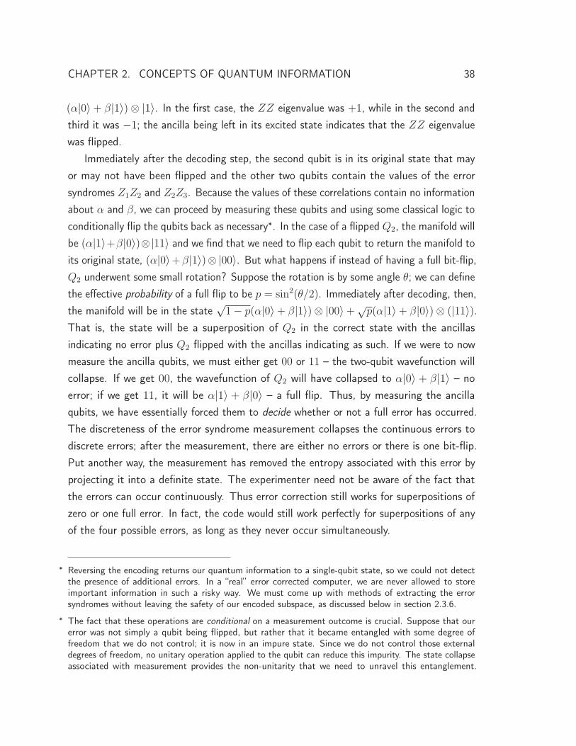
CHAPTER 2. CONCEPTS OF QUANTUM INFORMATION 38
(α|0〉 + β|1〉) ⊗ |1〉. In the first case, the ZZ eigenvalue was +1, while in the second andthird it was −1; the ancilla being left in its excited state indicates that the ZZ eigenvaluewas flipped.
Immediately after the decoding step, the second qubit is in its original state that mayor may not have been flipped and the other two qubits contain the values of the errorsyndromes Z1Z2 and Z2Z3. Because the values of these correlations contain no informationabout α and β, we can proceed by measuring these qubits and using some classical logic toconditionally flip the qubits back as necessary∗. In the case of a flipped Q2, the manifold willbe (α|1〉+β|0〉)⊗|11〉 and we find that we need to flip each qubit to return the manifold toits original state, (α|0〉+β|1〉)⊗ |00〉. But what happens if instead of having a full bit-flip,Q2 underwent some small rotation? Suppose the rotation is by some angle θ; we can definethe effective probability of a full flip to be p = sin2(θ/2). Immediately after decoding, then,the manifold will be in the state
√1 − p(α|0〉+ β|1〉)⊗ |00〉+√
p(α|1〉+ β|0〉)⊗ (|11〉).That is, the state will be a superposition of Q2 in the correct state with the ancillasindicating no error plus Q2 flipped with the ancillas indicating as such. If we were to nowmeasure the ancilla qubits, we must either get 00 or 11 – the two-qubit wavefunction willcollapse. If we get 00, the wavefunction of Q2 will have collapsed to α|0〉 + β|1〉 – noerror; if we get 11, it will be α|1〉 + β|0〉 – a full flip. Thus, by measuring the ancillaqubits, we have essentially forced them to decide whether or not a full error has occurred.The discreteness of the error syndrome measurement collapses the continuous errors todiscrete errors; after the measurement, there are either no errors or there is one bit-flip.Put another way, the measurement has removed the entropy associated with this error byprojecting it into a definite state. The experimenter need not be aware of the fact thatthe errors can occur continuously. Thus error correction still works for superpositions ofzero or one full error. In fact, the code would still work perfectly for superpositions of anyof the four possible errors, as long as they never occur simultaneously.
∗ Reversing the encoding returns our quantum information to a single-qubit state, so we could not detectthe presence of additional errors. In a “real” error corrected computer, we are never allowed to storeimportant information in such a risky way. We must come up with methods of extracting the errorsyndromes without leaving the safety of our encoded subspace, as discussed below in section 2.3.6.
∗ The fact that these operations are conditional on a measurement outcome is crucial. Suppose that ourerror was not simply a qubit being flipped, but rather that it became entangled with some degree offreedom that we do not control; it is now in an impure state. Since we do not control those externaldegrees of freedom, no unitary operation applied to the qubit can reduce this impurity. The state collapseassociated with measurement provides the non-unitarity that we need to unravel this entanglement.
CHAPTER 2. CONCEPTS OF QUANTUM INFORMATION 39
Figure 2.5: Autonomous QEC circuit. The three-qubit bit-flip code can be modified toeliminate the need for a measurement by implementing the classical logic operation with acoherent controlled-controlled-NOT gate and a non-unitary unconditional reset of the ancillaqubits.
Autonomous error correction
The previous section showed how measurement can be used to extract the entropy associatedwith an error from our quantum state. In practice, however, it can be challenging to extractinformation from our quantum state with high fidelity, perform a classical calculationwith that information, and manipulate our qubits conditioned on the result, all within atime brief compared to T2. Fortunately, it is possible to modify the code to eliminate theneed for this measurement by using a combination of a coherent multi-qubit operationand an unconditional qubit reset. As shown in Fig. 2.5, the first half of the code – theencoding, error, and decoding steps – are all the same as shown previously in Fig. 2.4. Thedifference comes after the unencoding and imprinting of the error syndromes in the ancillaqubits. There, we apply a three-qubit controlled-controlled NOT (ccNOT, also knownas Toffoli) gate which flips the target qubit if and only if both control qubits are excited.This implements the classical logic that would be used in the measurement-based case. Ifthe “protected” qubit were flipped, the ccNOT will flip it back since both ZZ eigenvalueswill be −1 and the ancillae will be left in their excited state after the unencoding. Thisapproach will still work with continuous errors because it acts coherently on each subspace.For example, if we again had |ψ〉 = √
1 − p(α|0〉+β|1〉)⊗|00〉+√p(α|1〉+β|0〉)⊗ (|11〉)
and applied our ccNOT on it, we would be left with the state |ψ′〉 =√1 − p(α|0〉 +
As soon we measure the ancilla, any entanglement with the bath is eliminated. As we will see later,unconditionally resetting a qubit can serve this purpose as well.
CHAPTER 2. CONCEPTS OF QUANTUM INFORMATION 40
β|1〉)⊗ |00〉+√p(α|0〉+ β|1〉)⊗ (|11〉) = (α|0〉+ β|1〉)⊗ (
√1 − p|00〉+√
p|11〉). Thatis, the protected qubit will be in its correct state and the ancillae will contain the entropyof the error.
At this point, the middle qubit will be in its original state (as long as there were zeroor one errors), but we still must return the ancillae to their ground state if we hope tore-encode and correct another error. Unfortunately, it is not possible to also do this withsome multi-qubit unitary gate. There are two arguments demonstrating this is true: first,a unitary operation cannot reduce the amount of entropy in a system since it would violatethe laws of thermodynamics (nor could the amount of entropy change since a unitary isinvertible and if entropy increased, its inverse must cause a corresponding decrease). Sincewe are treating these errors as random∗, they increase the entropy of our wavefunction,and therefore cannot be eliminated (only shuffled around, as we have done so far). Second,if the error we are correcting originates with an interaction with the environment – perhapsour qubit partially swapped an excitation with some other degree of freedom and is nowentangled – the error will not be correctable because our unitary by convention does notaddress that subsystem. Thus, we must introduce some non-unitary operation to extractthis entropy. One method is to reset the ancillae to the ground state |ψ〉 → |0〉 as shownin the final step of the code, by putting them in contact with a cold bath. (One exampleof this is described in section 6.2.4.)
Phase-flip correction
The code described thus far corrects only bit-flip errors, described by the Pauli operatorX. That represents only one of the possible rotations we can perform on a qubit. We canalso have Z errors. (Y errors can be thought of as simultaneous X and Z errors becauseiXZ = Y and do not count as an additional axis.) Moreover, Z errors are a much morecommon type of error for many types of qubits. For example, a superconducting qubit’sfrequency can sometimes be changed with applied flux and so noise in that parameterscrambles the phase of a superposition, producing a Z error. Fortunately, it is possible to
∗ “Errors” are not necessarily random. For example, a systematic under or over-rotation would look to thecode like a bit-flip error. Similarly, if we had some always-on coherent coupling to some other degree offreedom (e.g. the environment), it also would be correctable in principle, even though nothing about it istruly “random.” Its preferrable to actually eliminate such errors and reduce the overall error rate, but ifthat’s impossible, error correction could serve as a last line of defense. Nevertheless, there is no loss ofgenerality of labeling these systematic errors “entropy” since they are unknown from the point of view ofthe code.

CHAPTER 2. CONCEPTS OF QUANTUM INFORMATION 41
|ψ〉 • • H • •
E
• • H • • |ψ〉|0〉 •|0〉 •|0〉 H • • • • H •|0〉 •|0〉 •|0〉 H • • • • H •|0〉 •|0〉 •
Figure 2.6: Nine-qubit Shor code. Arbitrary single-qubit errors can be corrected byconcatenating the phase- and bit-flip codes. This is done by replacing each qubit used in thephase-flip code with three qubits that are bit-flip corrected. The measurement-free version isshown here; the eight bottom qubits would need to be reset at the end of this operation.
modify the bit-flip code to instead correct for phase-flips by changing coordinate systems.If immediately before (and after) the “error” portion of the code we applied a π/2 (−π/2)rotation around the y-axis (or a Hadamard), the code will correct for phase-flips instead ofbit-flips. This happens because the rotations will map Z errors to X errors and vice versa,since XY = iZ, or, more explicitly, Rπ/2
y RπzR
−π/2y = Rπ
x and Rπ/2y Rπ
xR−π/2y = Rπ
z (up toa global phase). These extra rotations can be commuted with the other rotations of thecode, so its requirements are no greater than the bit-flip code.
2.3.5 The Shor code
We have shown how the three-qubit code can correct bit-flip or phase-flip errors. Butwhat if we wish to correct both at the same time? In principle, being able to correct forboth X and Z errors (and thus also Y errors) would account for any possible error on asingle qubit, including particularly nasty errors like the depolarizing channel. We can seethat this is not possible to achieve with only three qubits by using a counting argument:we need one qubit to store the state we are protecting and two more classical bits toencode the four error syndromes of a single bit or phase flip. Thus, in order to correct forboth errors simultaneously we need more qubits. One conceptually straightforward way ofdoing this is the nine-qubit Shor code [17]. The idea of the Shor code is to concatenate
CHAPTER 2. CONCEPTS OF QUANTUM INFORMATION 42
the bit-flip and phase-flip codes together. As shown in Fig. 2.5, each “qubit” used in thephase-flip code will actually be a composite of three qubits which are themselves bit-flipcorrected, so any bit or phase flip of any one of the qubits will be corrected. The logicalbasis is then given by |0〉L = 1√
8(|000〉 + |111〉) ⊗ (|000〉 + |111〉) ⊗ (|000〉 + |111〉) and
|1〉L = 1√8(|000〉 − |111〉) ⊗ (|000〉 − |111〉) ⊗ (|000〉 − |111〉), where we would write our
encoded state as α|0〉L + β|1〉L. We can manipulate this logical qubit with the logicaloperators XL = XXXXXXXXX and ZL = ZZZZZZZZZ (which are not the sameas simultaneous rotations on each qubit individually – XL and ZL are nine-qubit gates).The error syndromes are given by the operators S1 = ZZIIIIIII, S2 = ZIZIIIIII,S3 = IIIZZIIII, S4 = IIIZIZIII, S5 = IIIIIIZZI, S6 = IIIIIIZIZ, S7 =
XXXXXXIII, and S8 = XXXIIIXXX, where the first six discriminate bit-flips ofeach individual physical qubit and the remaining two detect phase-flips of the three bit-flipcorrected composite qubits. This was one of the first error correcting codes discovered,but is unlikely to be the most practical given its relatively large overhead and complicatedlogical operations.
The five-qubit code
The Shor code is “inefficient” in that it can correct for more than one error on a singlequbit at a time. For example, because there is so much redundancy you could have abit-flip of one of all three “composite” qubits and still recover. It is actually possible tomake do with only five qubits to recover from an arbitrary single-qubit error [19] using theaptly named “five-qubit code.” The error syndromes (that is, stabilizer operators) are givenby S1 = XZZXI, S2 = IXZZX, S3 = XIXZZ and S4 = ZXIXZ, and the logicaloperators are XL = XXXXX and ZL = ZZZZZ. This is the smallest code possiblethat can correct any single-qubit error. Its efficiency can be proven by a simple countingargument. There are 3× 5 + 1 = 16 = 24 errors to detect (a Z, X, or Y error on eachqubit, or no error) and the information of one qubit to encode, thus giving us a total of4 + 1 = 5 required qubits.
Other error correcting codes
There are numerous other error correcting codes that have been discovered over the years.The 7-qubit Steane code is most similar to those we have previously discussed [18]. Thoughrequiring two more qubits than minimally necessary for an arbitrary single-qubit error, it
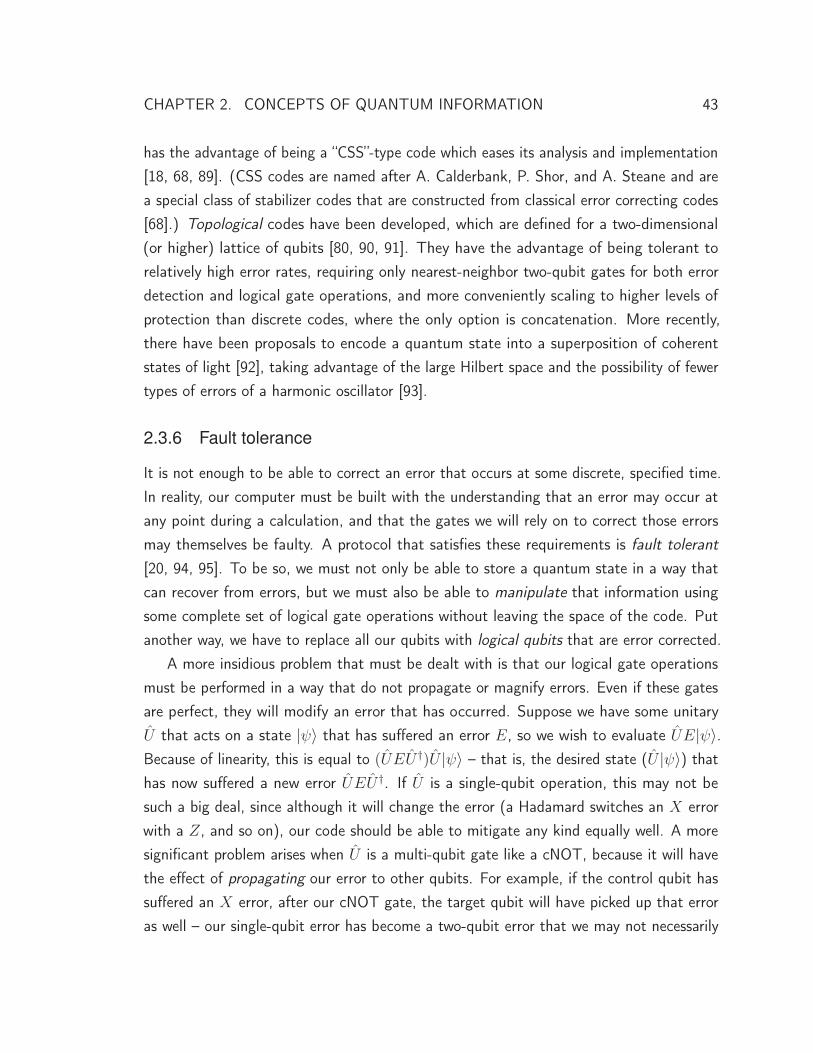
CHAPTER 2. CONCEPTS OF QUANTUM INFORMATION 43
has the advantage of being a “CSS”-type code which eases its analysis and implementation[18, 68, 89]. (CSS codes are named after A. Calderbank, P. Shor, and A. Steane and area special class of stabilizer codes that are constructed from classical error correcting codes[68].) Topological codes have been developed, which are defined for a two-dimensional(or higher) lattice of qubits [80, 90, 91]. They have the advantage of being tolerant torelatively high error rates, requiring only nearest-neighbor two-qubit gates for both errordetection and logical gate operations, and more conveniently scaling to higher levels ofprotection than discrete codes, where the only option is concatenation. More recently,there have been proposals to encode a quantum state into a superposition of coherentstates of light [92], taking advantage of the large Hilbert space and the possibility of fewertypes of errors of a harmonic oscillator [93].
2.3.6 Fault tolerance
It is not enough to be able to correct an error that occurs at some discrete, specified time.In reality, our computer must be built with the understanding that an error may occur atany point during a calculation, and that the gates we will rely on to correct those errorsmay themselves be faulty. A protocol that satisfies these requirements is fault tolerant[20, 94, 95]. To be so, we must not only be able to store a quantum state in a way thatcan recover from errors, but we must also be able to manipulate that information usingsome complete set of logical gate operations without leaving the space of the code. Putanother way, we have to replace all our qubits with logical qubits that are error corrected.
A more insidious problem that must be dealt with is that our logical gate operationsmust be performed in a way that do not propagate or magnify errors. Even if these gatesare perfect, they will modify an error that has occurred. Suppose we have some unitaryU that acts on a state |ψ〉 that has suffered an error E, so we wish to evaluate UE|ψ〉.Because of linearity, this is equal to (UEU †)U |ψ〉 – that is, the desired state (U |ψ〉) thathas now suffered a new error UEU †. If U is a single-qubit operation, this may not besuch a big deal, since although it will change the error (a Hadamard switches an X errorwith a Z, and so on), our code should be able to mitigate any kind equally well. A moresignificant problem arises when U is a multi-qubit gate like a cNOT, because it will havethe effect of propagating our error to other qubits. For example, if the control qubit hassuffered an X error, after our cNOT gate, the target qubit will have picked up that erroras well – our single-qubit error has become a two-qubit error that we may not necessarily
CHAPTER 2. CONCEPTS OF QUANTUM INFORMATION 44
encode correct decode
|ψ〉 • •E
• • X • • |ψ〉|0〉 • X |0〉|0〉 • X |0〉
|0〉 ���
|0〉 ���
� � � � ���������
��������
� � � � �
� � � � � � � � � � � � � ���������������
��������������� � � � � � � � � � � � � �
� � � � ���������
��������
� � � � �
Figure 2.7: Fault-tolerant three-qubit bit-flip code. Rather than decoding the qubitsafter the error, one can use two additional ancillae to extract and measure the error syndromes.This way the quantum information is always protected from bit-flip errors. Combined withlogical gate operations, this constitutes a fault-tolerant implementation of the three-qubitcode.
be able to correct. In order to be fault-tolerant, then, we must be very careful with ourmulti-qubit gates so as to avoid this problem.
The solutions to all these problems will not be fully explained here, but we can getthe flavor of the necessary changes by looking at how we might modify the three-qubitcode. Since we can never leave the code space, we no longer have the luxury of recyclingthe ancilla qubits to also extract the error syndromes. As shown in Fig. 2.7, we insteadmeasure the correlations Z1Z2 and Z2Z3 with two additional ancillae through the use ofcontrolled-NOT gates. In addition to not having our logical qubit leave the subspace, thishas the further advantage of potentially allowing us to measure the syndromes severaltimes before making a decision, since the logical qubit is an eigenstate of those operators.This is helpful if our cNOT or measurement operations are not perfect. It is also inprinciple possible to make a fault-tolerant version of autonomous error correction wheremeasurements are not necessary, but it requires a great deal more overhead since the“classical” logic can no longer be assumed to be perfect.
2.4 Conclusions
This chapter was intended to serve as a brief introduction to quantum information sciencefor people with a background in physics but no particular knowledge of the subject. We

CHAPTER 2. CONCEPTS OF QUANTUM INFORMATION 45
started with a survey of the tools and language used in quantum information: the Blochsphere, Pauli matrices and operators, the density matrix, and entanglement, to name a few.This led into a discussion of what makes quantum information processing so powerful butalso that harnessing that power to run quantum algorithms has many stringent hardwarerequirements. Finally, we showed why quantum information is particularly sensitive toerrors, and explained the simplest model of how we might correct them without losing theiradvantages. We concluded with a discussion of more sophisticated codes that can correctfor arbitrary errors and have different hardware and parameter requirements, and gavean outline of fault tolerant error correction. With the tools introduced here established,we can now proceed with an explanation of our particular implementation of quantuminformation processing. In the next chapter, we discuss superconducting qubits coupled tomicrowave resonators, known as circuit quantum electrodynamics, with the goal of layingthe framework to present our recent experimental achievements.

CHAPTER 3
Superconducting Qubits and cQED
The previous chapter introduced the requirements that a quantum computer mustsatisfy; however, there was no corresponding statement about the particular physical
manifestation of such a machine. In fact, significant experimental progress has been madeusing a variety of systems [96] including nuclear spins [97, 98], trapped ions [26, 27, 29–31],linear optics [99, 100], solid state quantum dots [40–44], diamond color centers [44, 46–48], and superconducting circuits [49]. In addition, there have been dozens of proposals[101] for additional systems like topologically protected qubits [102–104]. Demonstratingthe basic building blocks of quantum information science like single-qubit control andon-demand entanglement is a lot different than mastering a system that could be scaledto a fault-tolerant million-qubit system, however. Thus, the history of quantum computinghas seen the rise and fall of several technologies at the experimental forefront. Thoughliquid-state NMR systems were always known not to be scalable [25], they made rapid initialprogress before being superseded by trapped ions. Recent advances with superconductingcircuits[61, 62] and quantum dots [42, 43] are now threatening the primacy of ions. Thefield is increasingly concerned not only with basic quantum information experiments, butalso with which system has a chance to scale to the large number of qubits required toperform calculations or simulations not otherwise possible.
This thesis reports on one of the most promising technologies: superconducting qubits.
47
CHAPTER 3. SUPERCONDUCTING QUBITS AND CQED 48
Compared to its competitors, superconducting circuits have certain advantages, such asbeing relatively simple to fabricate using standard lithography techniques [105], havingall-electrical quantum control using microwave light fields [52, 106], and large, controllablenonlinearities at small energy scales [107]. They require being cooled in a helium dilutionrefrigerator to milliKelvin temperatures, however, and until recently there were majorquestions about the limits of their coherence. There is still a lot of work necessary to builda scalable quantum architecture with these devices, but progress has been very rapid andthere is no known reason that will inhibit this technology from advancing further. Moreover,it has enabled a new class of quantum physics experiments [107–111] that, in addition tobeing useful for information processing, are intrinsically interesting and beautiful.
This chapter begins with a theoretical introduction to the physics of superconductingqubits and the architecture with which we study them. These two topics have beendiscussed in great detail in previous theses [112–114] and papers [106, 115, 116], and sowe summarize rather than exhaustively derive those results. We focus on the particular kindof qubit, the transmon [115, 117], that we are studying in our lab. It is conveniently modeledas a nonlinear LC oscillator that has non-degenerate transition frequencies between higherexcited states. These additional levels play an important role in generating entanglement, aswill be discussed in chapter 7. We couple these qubits to standing-wave modes of microwaveresonators in the circuit quantum electrodynamics (cQED) architecture [118, 119]. Thedynamics of cQED are described by the Jaynes-Cummings Hamiltonian [120]. While beingstraightforward to derive, it must be approximated and transformed in order to mostclearly see the properties we regularly take advantage of for readout, single-qubit gates,and qubit-qubit coupling. We complete this section by discussing dissipation and thestrong dispersive limit, which defines a regime of parameter space where even high-orderqubit-cavity coupling terms dominate over decoherence, enabling additional control throughthe use those effects.
Many of our devices employ flux bias lines (FBLs), which are current-carrying wiresused to thread magnetic flux through the qubit SQUID loop. They allow us to tunequbit transition frequencies in-situ and have been used successfully in the planar cQEDarchitecture [55, 121]. The final section of this chapter will discuss our recent extensionof FBLs to the 3D cQED architecture. We will show how to calculate the flux couplingthat we can expect for a given geometry, which has been a concern due to the screeningeffects of the superconducting 3D box, and show that for reasonable geometries it shouldbe possible to thread a flux quantum with a sufficiently small amount of current. Doing
CHAPTER 3. SUPERCONDUCTING QUBITS AND CQED 49
so requires a drastic expansion of the size of the FBL and the SQUID loop that greatlyincreases the capacitance between the two, creating a new channel for qubit decay. Weshow how to calculate the expected qubit lifetime using an effective circuit model and howwe can add simple filtering to fix the problem.
3.1 Superconducting qubits
One thing that distinguishes superconducting qubits from virtually all of their competitorsis the fact that the quantum degree of freedom is not that of a single or small numberof discrete particles. Instead, superconducting qubits employ the collective motion of amacroscopic number of paired electrons known as Cooper pairs. These particles havecondensed into a single collective ground state. Electrical circuits built using superconduc-tors will exhibit quantum behavior with energy levels set by their geometric parameters.They can in principle be lossless if we limit ourselves to dissipationless elements like thecapacitor and the inductor. However, because these are both linear elements, the onlyHamiltonian we could engineer with them is the harmonic oscillator. They would havehave precisely evenly spaced levels and the only free parameter is the frequency of thatoscillator. A system must have individually addressable transitions if we intend to controltwo of its levels as a qubit; linear elements are insufficient.
To our great fortune, superconductors are endowed with the only known simultaneouslynonlinear and non-dissipative circuit element∗, the Josephson junction [122, 123]. It is thesource of anharmonicity used by all types of superconducting qubits. There are severalways of making a Josephson junction, which is most generally any weak link betweentwo superconductors. By far the most common method is via two superconducting wiresseparated by a thin insulating oxide. Cooper pairs may coherently tunnel across this barrier,which leads to a phase difference φ between the macroscopic wavefunction on one side ofthe barrier compared with the other. The condensates on either side are in the ground stateof the BCS Hamiltonian, so this phase difference is the only possible low-energy degree offreedom. The tunneling supercurrent is given by I = Icsinφ(t), where the critical currentIc is the maximum current that may flow through the junction and is set by parameterslike the effective barrier transparency. The phase φ(t) evolves in time in the presence of apotential difference V across the junction according to
�∂φ
∂t= 2eV. (3.1)

CHAPTER 3. SUPERCONDUCTING QUBITS AND CQED 50
Taking the full time derivative of I, we have
I = (Iccosφ)∂φ
∂t=
2eV Ic�
cosφ. (3.2)
We note that this equation looks like the inductor relationship V = −LI with a Josephsoninductance given by
LJ =�
2eV Iccosφ=
Φ0
2πIccosφ(3.3)
where Φ0 = h/2e is the magnetic flux quantum. Thus, the Josephson junction can bethought of as an inductor with an inductance that depends on φ, and thus the appliedcurrent, and is therefore nonlinear.
3.1.1 The Transmon qubit
In the early days of superconducting quantum information science, there was a proliferationof qubit circuit topologies that were classified as flux [129–131], phase [132, 133], andcharge qubits [50, 134, 135] based on which degree of freedom was a good quantum number.As time went on, these distinctions became less and less relevant as “hybrid” superconductingqubits were developed that had better properties (e.g. decreased susceptibility to specificsources of noise) and whose eigenstates were no longer number states of any of the threequantities [52, 115, 117]. One such hybrid qubit is known as the transmon. Thoughnormally classified as a charge qubit, it enjoys an exponentially suppressed sensitivity tocharge noise because its eigenstates are superpositions of several charge states [115]. It isoften sufficient to consider this qubit as a slightly anharmonic LC oscillator, though as wewill see, calculating the detailed level structure requires a more careful treatment.
The Cooper-pair box
The transmon qubit is a derivative of the Cooper-pair box qubit (CPB). The CPB istopologically simple, consisting of two superconducting islands connected by a Josephsonjunction [50, 134]. Cooper pairs may tunnel across this junction, and since there is onlyone path for this transit, the number of tunneled pairs is an integer quantity. This also
∗ One possibly exception to this statement is the field of cavity quantum optomechanics, where the low-energy interaction between light and mechanical objects is studied [124–128]. The radiation pressureof light couples to the mechanical motion of some oscillator, which can endow the Hamiltonian with anonlinearity.
CHAPTER 3. SUPERCONDUCTING QUBITS AND CQED 51
implies that the junction phase φ is “compact” or periodic in 2π. (This would not be true if,for example, the junction was shorted out by an inductor as it is with a phase qubit. There,the potential energy landscape has an overall φ2 dependence on top of the Josephsonsinusoid. φ is then non-compact due to the closed-loop topology of the circuit.) There aretwo relevant energy scales: EC = e2
2CΣ, the charging energy of a single electron stored on
the capacitance, and EJ = ICΦ0
2π, the energy associated with an electron tunneling across
the junction. CΣ = Cg + CJ is the total capacitance of the CPB to ground, given by thesum of the geometric capacitance and the capacitance of the Josephson junction itself.The CPB Hamiltonian is then
H = 4EC(n − ng)2 − EJcosφ (3.4)
where n is the integer number of Cooper pairs that have tunneled through the junction,ng is some offset “gate” charge representing an external voltage bias, and φ is the phaseacross the junction and is periodic in 2π. n and φ are canonically conjugate variables,where n = ∂
∂φand [n, e±iφ] = ±e±iφ ∗.
We can build some intuition for this Hamiltonian with a physical analog of a chargedquantum rotor, following the argument of Koch et al. [115]. Suppose we have somepoint-mass m attached to a massless rod of length l, which is free to rotate around a fixedpivot. The potential energy of the mass in a uniform gravitational field is V = −mglcos(φ),where φ is the angle of the rod relative to its equilibrium position. Angular momentum isgiven by Lz = (�r × �p) · z = i� ∂
∂φ, so our full Hamiltonian is
Hrotor =L2z
2ml2− mglcosφ. (3.5)
Since Lz/� has integer eigenvalues, we can map n ↔ Lz/�, EJ ↔ mgl, EC ↔ �2/8ml2,and we find that this is identical to Eq. 3.4 with ng = 0. We can add that term bystipulating that the mass carries some charge and is in a uniform magnetic field parallelto the rotor’s pivot, and thus �p → �p − q �A, giving Lz → Lz +
12qB0l
2, where the vectorpotential A = B0(−y, x, 0)/2. This gives ng ↔ qB0l
2/2�, completing our one-to-onemapping of the Cooper-pair box Hamiltonian to the charged quantum rotor.
∗ If φ is non-compact, we would have [n, φ] = 1. When φ is compact, only operators like eiφ that respectthe periodicity of φ are valid.

CHAPTER 3. SUPERCONDUCTING QUBITS AND CQED 52
8
6
4
2
0
Ener
gy /E
C
-1.0 -0.5 0.0 0.5 1.0
EJ/EC = 0
|0> |1> |2>
10
8
6
4
2
0
-2
-1.0 -0.5 0.0 0.5 1.0
EJ/EC = 5
|0> |1> |2>
8
4
0
-4
Ener
gy /E
C
-1.0 -0.5 0.0 0.5 1.0Gate charge ng
EJ/EC = 10
|0> |1> |2>
-90
-80
-70
-60
-50
-40
-30
-1.0 -0.5 0.0 0.5 1.0Gate charge ng
EJ/EC = 100
|0> |1> |2>
f01
f12
Figure 3.1: Transmon energies as a function of gate charge. We plot the energy ofthe solutions to Eq. 3.4 as a function of gate charge ng. We show the results for variousvalues of EJ/EC , demonstrating the reduction in gate charge sensitivity.
Transmon regime
The gate charge ng is actually a major nuisance because its value is subject to chargenoise. Electrons drifting around in the environment will cause it to change at random. Ifthat changes the transition frequency of our qubit, it will induce dephasing. Fortunately,we can suppress our sensitivity to gate charge by operating our qubit in the “transmon”regime where the ratio EJ/EC is large. In this limit, variation in transition frequencybetween two subsequent levels as a function of gate charge∗ scales as e−
√8EJ/EC . The
cost, a small EC , reduces the anharmonicity of the qubit. However, this effect scales onlygeometrically with EC whereas our sensitivity to charge noise scales exponentially – ahuge net win [115]. We show numerically-evaluated energies for various values of EJ/EC
CHAPTER 3. SUPERCONDUCTING QUBITS AND CQED 53
as a function of ng in Fig. 3.1. This shows that for low values of EJ/EC the transitionenergies depend strongly on ng, but for larger values the dependence flattens out.
Large EJ/EC corresponds to limiting our junction to small phase excursions fromφ = 0. For our rotor model, this is imposed when both the gravitational pull and momentof inertia are very large, so the angle φ only experiences small fluctuations. In this limit,we can expand the cosine potential as H = H0 + V , where H0 is a linear term given by4EC n
2 + EJ
2φ2 and V is the perturbation
V = EJ
(− 1
4!φ4 +
1
6!φ6 + ...
). (3.6)
We identify H0 as a simple harmonic oscillator with frequency �ω =√8EJEC . As we
mentioned earlier, to zeroth order, the transmon is an LC oscillator with the Josephsonjunction serving as a large linear inductor. Importantly, the gate charge ng does not enterinto this calculation. By limiting ourselves to small values of φ, the boundary conditionthat φ = φ+ 2π becomes irrelevant, meaning that φ can be treated as non-compact. Weare free to impose vanishing boundary conditions on our wavefunction for φ → ∞. Thistransforms the conjugate momentum n from an integer-valued discrete quantity into acontinuous quantity and we can therefore neglect the offset term ng. Limiting ourselves tosmall phase fluctuations corresponds to large charge fluctuations, which in turn dispersethe discreteness of charge [136].
We continue our calculation in second quantization with the substitution φ = φZP(a+
a†), where φ2ZP = �ω
2EJ=√
2EC
EJ. Plugging this in, we have H0 = �ωa†a, the normal
harmonic oscillator equation, and V ≈ −112EC(a + a†)4. Expanding the term (a + a†)4
and dropping rapidly-rotating terms like a†a† (the rotating-wave approximation), we getV ≈ −EC
2(a†a†aa+ 2a†a) [137]. Combining terms, we find that the oscillator frequency
has been renormalized to�ω′ =
√8EJEC − EC (3.7)
and has an anharmonicity given by
α = −EC . (3.8)
∗ In the WKB approximation, the Mathieu characteristic values can be approximated to give the charge
dispersion for the mth level of the transmon as εm ∼ (−1)mEC24m+5
m!
√2π
(EJ
2EC
)m2 + 3
4
e−8√
8EJ/EC .Note that the size of charge dispersion increases with the excitation level.
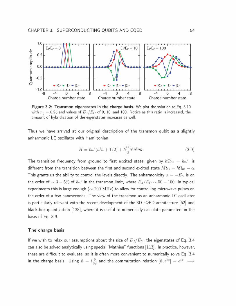
CHAPTER 3. SUPERCONDUCTING QUBITS AND CQED 54
-4 0 4 8Charge number state
|0> |1> |2>
EJ/EC = 100
-4 0 4 8Charge number state
|0> |1> |2>
EJ/EC = 10
-1.0
-0.5
0.0
0.5
1.0
Qua
ntum
am
plitu
de
-8 -4 0 4 8Charge number state
|0> |1> |2>
EJ/EC = 0
Figure 3.2: Transmon eigenstates in the charge basis. We plot the solution to Eq. 3.10with ng = 0.25 and values of EJ/EC of 0, 10, and 100. Notice as this ratio is increased, theamount of hybridization of the eigenstates increases as well.
Thus we have arrived at our original description of the transmon qubit as a slightlyanharmonic LC oscillator with Hamiltonian
H = �ω′(a†a+ 1/2) + �α
2a†a†aa. (3.9)
The transition frequency from ground to first excited state, given by �Ω01 = �ω′, isdifferent from the transition between the first and second excited state �Ω12 = �Ω01 − α.This grants us the ability to control the levels directly. The anharmonicity α = −EC is onthe order of ∼ 3− 5% of �ω′ in the transmon limit, where EJ/EC ∼ 50− 100. In typicalexperiments this is large enough (∼ 200 MHz) to allow for controlling microwave pulses onthe order of a few nanoseconds. The view of the transmon as an anharmonic LC oscillatoris particularly relevant with the recent development of the 3D cQED architecture [62] andblack-box quantization [138], where it is useful to numerically calculate parameters in thebasis of Eq. 3.9.
The charge basis
If we wish to relax our assumptions about the size of EJ/EC , the eigenstates of Eq. 3.4can also be solved analytically using special “Mathieu” functions [113]. In practice, however,these are difficult to evaluate, so it is often more convenient to numerically solve Eq. 3.4in the charge basis. Using n = i ∂
∂φand the commutation relation [n, eiφ] = eiφ =⇒

CHAPTER 3. SUPERCONDUCTING QUBITS AND CQED 55
eiφ|n〉 = |n+ 1〉, we rewrite the Hamiltonian as
H = 4EC
N∑j=−N
(j − ng)2|j〉〈j| − EJ
N−1∑J=−N
|j + 1〉〈j| + |j〉〈j + 1| (3.10)
where we truncate the Hilbert space at some size N large enough to encompass the levelswe are interested in evaluating. In this representation, the underlying tunneling of Cooperpairs is clear, with the first term corresponding to the capacitive energy stored in thecharge configuration and the second term to the tunneling across the junction. We writethe solution to this equation in the transmon basis which diagonalizes it, given by
Hq = �∑k
ωk|k〉〈k| (3.11)
where |k〉 are the exact solutions to the CPB Hamiltonian (e.g. in the φ basis, the Mathieufunctions) and ωk = Ek� are the eigenenergies. We will often approximate the |k〉 withthe numerical solutions of equation 3.10, with which we can compute much faster. Severalsuch solutions for various values of EJ/EC are shown in Fig. 3.2.
When the higher excited states are not important, we can approximate the transmonoscillator as a two-level qubit by restricting our sum to only the ground and first excitedstate. Ignoring the existence of the higher levels (for example, taking the limit that theanharmonicity goes to infinity), we approximate the qubit Hamiltonian as a spin-1/2particle with
Hq =�
2ωqσz. (3.12)
Here, we would assign ωq = ω′, the value that we calculated in the previous section. Thisapproach lends itself more readily to the language of quantum information science, as wediscussed in chapter 2.
Flux sensitivity
Both the Cooper-pair box and the transmon are often designed with a pair of Josephsonjunctions connecting the islands rather than only one. This configuration, known as asuperconducting quantum interference device or SQUID, allows for the tuning of theeffective EJ by changing the magnetic flux Φ threading through the loop formed by thetwo junctions. The Josephson contribution to the CPB Hamiltonian with two junctions is
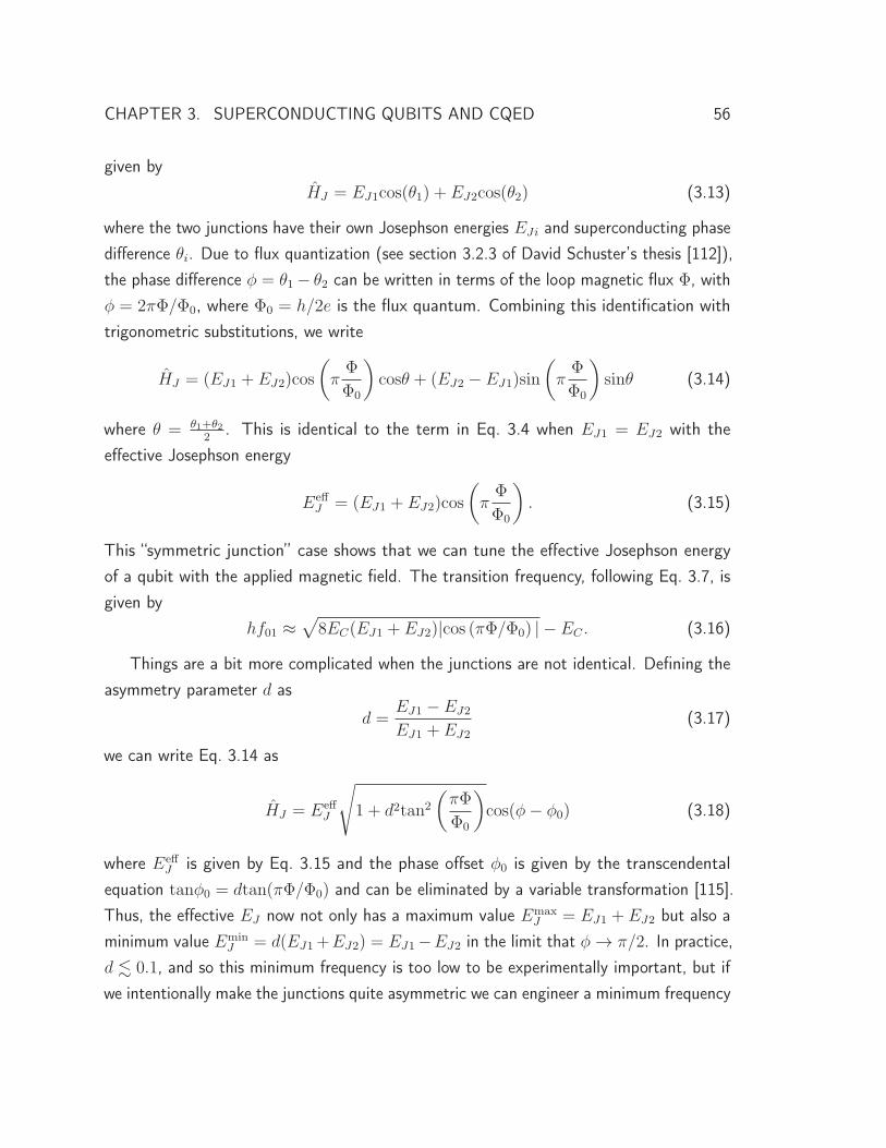
CHAPTER 3. SUPERCONDUCTING QUBITS AND CQED 56
given byHJ = EJ1cos(θ1) + EJ2cos(θ2) (3.13)
where the two junctions have their own Josephson energies EJi and superconducting phasedifference θi. Due to flux quantization (see section 3.2.3 of David Schuster’s thesis [112]),the phase difference φ = θ1 − θ2 can be written in terms of the loop magnetic flux Φ, withφ = 2πΦ/Φ0, where Φ0 = h/2e is the flux quantum. Combining this identification withtrigonometric substitutions, we write
HJ = (EJ1 + EJ2)cos
(πΦ
Φ0
)cosθ + (EJ2 − EJ1)sin
(πΦ
Φ0
)sinθ (3.14)
where θ = θ1+θ22
. This is identical to the term in Eq. 3.4 when EJ1 = EJ2 with theeffective Josephson energy
EeffJ = (EJ1 + EJ2)cos
(πΦ
Φ0
). (3.15)
This “symmetric junction” case shows that we can tune the effective Josephson energyof a qubit with the applied magnetic field. The transition frequency, following Eq. 3.7, isgiven by
hf01 ≈√
8EC(EJ1 + EJ2)|cos (πΦ/Φ0) | − EC . (3.16)
Things are a bit more complicated when the junctions are not identical. Defining theasymmetry parameter d as
d =EJ1 − EJ2
EJ1 + EJ2
(3.17)
we can write Eq. 3.14 as
HJ = EeffJ
√1 + d2tan2
(πΦ
Φ0
)cos(φ − φ0) (3.18)
where EeffJ is given by Eq. 3.15 and the phase offset φ0 is given by the transcendental
equation tanφ0 = dtan(πΦ/Φ0) and can be eliminated by a variable transformation [115].Thus, the effective EJ now not only has a maximum value Emax
J = EJ1 + EJ2 but also aminimum value Emin
J = d(EJ1+EJ2) = EJ1 −EJ2 in the limit that φ → π/2. In practice,d � 0.1, and so this minimum frequency is too low to be experimentally important, but ifwe intentionally make the junctions quite asymmetric we can engineer a minimum frequency
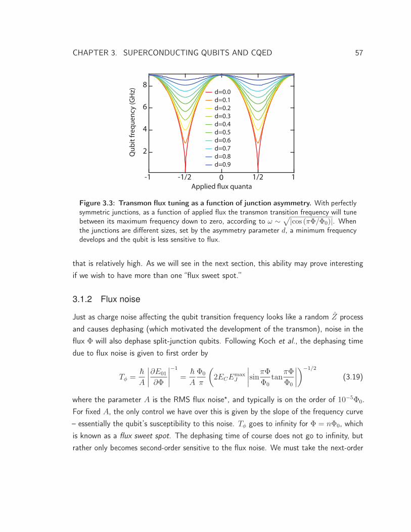
CHAPTER 3. SUPERCONDUCTING QUBITS AND CQED 57
8
6
4
2
2.01.51.00.50.0
d=0.0 d=0.1 d=0.2 d=0.3 d=0.4 d=0.5 d=0.6 d=0.7 d=0.8 d=0.9
Qub
it fr
eque
ncy
(GH
z)
-1 10-1/2 1/2Applied flux quanta
Figure 3.3: Transmon flux tuning as a function of junction asymmetry. With perfectlysymmetric junctions, as a function of applied flux the transmon transition frequency will tunebetween its maximum frequency down to zero, according to ω ∼ √|cos (πΦ/Φ0)|. Whenthe junctions are different sizes, set by the asymmetry parameter d, a minimum frequencydevelops and the qubit is less sensitive to flux.
that is relatively high. As we will see in the next section, this ability may prove interestingif we wish to have more than one “flux sweet spot.”
3.1.2 Flux noise
Just as charge noise affecting the qubit transition frequency looks like a random Z processand causes dephasing (which motivated the development of the transmon), noise in theflux Φ will also dephase split-junction qubits. Following Koch et al., the dephasing timedue to flux noise is given to first order by
Tφ =�
A
∣∣∣∣∂E01
∂Φ
∣∣∣∣−1
=�
A
Φ0
π
(2ECE
maxJ
∣∣∣∣sinπΦΦ0
tanπΦ
Φ0
∣∣∣∣)−1/2
(3.19)
where the parameter A is the RMS flux noise∗, and typically is on the order of 10−5Φ0.For fixed A, the only control we have over this is given by the slope of the frequency curve– essentially the qubit’s susceptibility to this noise. Tφ goes to infinity for Φ = nΦ0, whichis known as a flux sweet spot. The dephasing time of course does not go to infinity, butrather only becomes second-order sensitive to the flux noise. We must take the next-order
CHAPTER 3. SUPERCONDUCTING QUBITS AND CQED 58
derivative of ω(Φ), giving
Tφ =
∣∣∣∣π2A2
�
∂2E01
∂Φ2
∣∣∣∣−1
Φ=0
=�Φ2
0
A2π4√
2EmaxJ EC
. (3.20)
At a flux bias of Φ = Φ0/4, A = 10−5Φ0, EJ = 30 GHz, and EC = 350 MHz, Eq. 3.19gives Tφ ∼ 1 μs, while at the flux sweet spot Φ = 0, these same parameters give Tφ ∼ 3 ms.Thus, it is always preferable to operate as close as possible to a flux sweet spot; a lotof effort has gone into engineering fmax for this exact reason. As we saw in the previoussection, any amount of junction asymmetry gives rise to two sweet spots. In principle, onecould choose the junction sizes carefully to set these two frequencies at experimentallyrelevant values.
3.2 Circuit quantum electrodynamics
The field of circuit quantum electrodynamics (cQED) concerns the study of superconductingqubits that are strongly coupled to a mode of light [106, 118]. Conventionally, this mode wasa standing wave in a 1-dimensional microwave-frequency transmission line [118, 119, 121],but more recently the resonant modes of a 3D box have supplanted that role [62]. Thismode, commonly known as the “cavity” in reference to the older and recently Nobelprize-winning field of cavity quantum electrodynamics, fills many important roles. First,because the frequency of the cavity mode is sensitive to the state of the qubit(s), wecan infer those states with a cavity transmission measurement [58, 116]. Second, thecavity gives us an easy way to perform single-qubit rotations with resonant microwavetones [53]. Third, as we will see in section 6.2.1, it protects the qubit from spontaneousdecay by changing the density of photon states [139]. Fourth, and finally, it mediatesqubit-qubit coupling via a virtual coupling [119, 121]. We do not seek to re-derive all theproperties of cQED here given the plentiful pre-existing resources that do an excellent job[106, 112–115, 137]. We will instead briefly summarize the results of these sources thatwe will reference in later chapters.
∗ Treating flux noise properly is a bit difficult. Equation 3.19 is a statement that T−1φ = δωRMS = ∂ω
∂ΦΦRMS.Our job is to define ΦRMS in a reasonable way. Since we are assuming the noise follows a 1/f frequencydependence, we have to define some frequency range that we care about. Thus, Φ2
RMS =∫ fmax
fmin
A2
f df =
A2ln( fmax
fmin). This logarithmic factor is of order unity, so we usually approximate ΦRMS = A. Strictly
speaking, however, A sets only the scale of noise and not its precise magnitude.
CHAPTER 3. SUPERCONDUCTING QUBITS AND CQED 59
3.2.1 Harmonic oscillators
Both transmission lines and 3D cavity modes are, in the absence of a qubit, linear harmonicoscillators∗. The Hamiltonian of a single harmonic oscillator is given by
HHO = �ω(a†a+ 1/2
)= �ω
(N + 1/2
)(3.21)
where a† and a are the raising and lowering operators and N = a†a is the number operator.The operators satisfy the relation [a, a†] = 1. We can define a number basis |n〉 which isan eigenvector of the number operator with N |n〉 = n|n〉. We can also define a conjugateset of variables, charge Q and magnetic flux Φ (or equivalently, position and momentum)as Q = −iQZPF(a− a†) and Φ = ΦZPF(a+ a†), where QZPF and ΦZPF are the magnitudeof the zero-point fluctuations of each variable and can be defined in terms of the physicalparameters of the oscillator. These variables correspond to physical observables of thecharge on the capacitor and the flux through the inductor of the effective circuit of theoscillator, and obey the relation [Φ, Q] = i�.
We can calculate the eigenstates of this Hamiltonian in second quantization [140].First, we note that a†|n〉 = √
n+ 1|n + 1〉 and a|n〉 = √n|n − 1〉, which implies that
a|0〉 = 0. Writing a = 12
(Φ
ΦZPF+ i Q
QZPF
), and noting that Q = �
i∂
∂Φ, we have
〈Φ|a|0〉 = 1
2〈Φ|
(Φ
ΦZPF
+ iQ
QZPF
)|0〉 = 1
2〈Φ|
(Φ
ΦZPF
+i
QZPF
�
i
∂
∂Φ
)|0〉
=1
2
(Φ
ΦZPF
〈Φ|0〉 + �
QZPF
∂
∂Φ〈Φ|0〉
)= 0
(3.22)
where in the second line we have used 〈Φ|Φ|0〉 = Φ〈Φ|0〉 and 〈Φ| ∂
∂Φ|0〉 = ∂
∂Φ〈Φ|0〉.
∗ See, for example, Chapter 2 of Steven Girvin’s 2011 Les Houches notes for a modern approach to howcircuits are quantized [137]. Other useful resources are Chapter 3 of David Schuster’s 2008 thesis [112]and Chapter 2 of Lev Bishop’s 2010 thesis [113]. Circuit quantization involves assembling a Lagrangianfor the system following an explicit set of instructions and applying a Legendre transformation to get theHamiltonian. A quantum LC oscillator is found to have the Lagrangian L(φ, φ) = Cφ2
2 − φ2
2L , where φis the flux in the inductor and L and C are the inductance and capacitance of the circuit, respectively.From this, the Hamiltonian is found to be the common harmonic oscillator with H = q2
2C + φ2
2L , with q theoperator for charge on the capacitor. This can be written in terms of raising and lowering operators as
H = �ω(a†a+ 1
2
)with [a, a†] = 1, φ =
√�Z2 (a+ a†), q = −i
√�
2Z (a− a†), ω = 1√LC
, and Z =√
LC .

CHAPTER 3. SUPERCONDUCTING QUBITS AND CQED 60
Solving, we find the first-order single-variable differential equation
∂
∂Φ〈Φ|0〉 = −QZPF
�ΦZPF
Φ〈Φ|0〉 (3.23)
whose solution is given by the gaussian
〈Φ|0〉 = Ne−QZPF2�ΦZPF
Φ2
= Ne− Φ2
2Φ2ZPF (3.24)
with the normalization factor N =(
QZPF
π�ΦZPF
)1/4
and noting that QZPFΦZPF = �. Wecan also get the higher excited states of the harmonic oscillator by applying the raisingoperator a† = 1
2
(Φ
ΦZPF− i Q
QZPF
), so that
〈Φ|n〉 = 1√n!
〈Φ|(a†)n|0〉
=1
2n√n!
(Φ
ΦZPF
− �
QZPF
∂
∂Φ
)n(QZPF
π�ΦZPF
)1/4
e−QZPF2�ΦZPF
Φ2
.
(3.25)
Omitting normalization, we find for example
〈Φ|1〉 = Φe−QZPF2�ΦZPF
Φ2
. (3.26)
In the absence of some nonlinearity, this quantization of photon number is not physicallyobvious. The classical controls that we possess over a cavity are not sources of a definitenumber of photons, but rather perform what is known as a displacement on the oscillator.This is because the oscillator’s levels are exactly evenly spaced so we cannot addressindividual transitions. For example, if we apply a resonant drive to a cavity in its groundstate, we will initially transfer population from |0〉 to |1〉. However, as soon as there ispopulation in |1〉, transitions to |2〉 are possible, which then turns on transitions to |3〉,and so on. Thus, we can only create some Poisson-distributed superposition of numberstates. The unitary displacement operator describing this process is given by
D(α) = eαa†−α∗a. (3.27)
The parameter α is a complex number, with α = |α|eiφ. Working in the photon numberbasis, if we apply this displacement operator on the ground state, we will produce a

CHAPTER 3. SUPERCONDUCTING QUBITS AND CQED 61
coherent state
D(α)|0〉 = |α〉 = e−|α|22
∞∑n=0
αn
√n!
|n〉. (3.28)
This state is an eigenstate of the lowering operator, with
a|α〉 = α|α〉. (3.29)
A real-valued displacement corresponds to adding a constant to the flux (position) coordi-nate of the harmonic oscillator, while an imaginary value corresponds to adding charge(momentum). For example, a displaced ground state wavefunction is given by
〈Φ|D(λ)|0〉 = 〈(Φ − λ)|0〉 = 〈Φ|λ〉 = ψλ(Φ) (3.30)
where λ is some real-valued displacement along the flux axis. As a function of time, adisplaced state will oscillate between being displaced in flux and in charge, with
a(t)|α〉 = eiωtα|α〉=⇒ |α(t)〉 = |αeiωt〉.
(3.31)
It can be shown that any possible linear drive of the form Hd = f(t)(a+ a†) can only everproduce a coherent state, independent of the form of f(t)∗.
Both the transmission line and 3D box have higher modes (e.g. the first mode of thetransmission line has voltage nodes only at the capacitors, but higher modes will haveadditional nodes), so we can expand our treatment to explicitly take them into accountwith
HnHO = �∑n
ωn
(a†nan + 1/2
)(3.32)
where ωn is the frequency of the nth mode. Enumerating these modes can be doneanalytically in the case of a transmission line†, but is more complicated with a 3D box andgenerally requires a numerical simulation of the actual box geometry. These higher modesare often neglected, but understanding them can be important because they can be a
∗ As a corollary, if we ever want to have some interesting “non-classical” state of light, we require somesort of nonlinearity to get out of coherent state purgatory. A qubit turns out to be a great source ofnonlinearity, with several recent results creating and detecting photon number Fock states [109, 141] andSchrödinger cat states [107, 142].
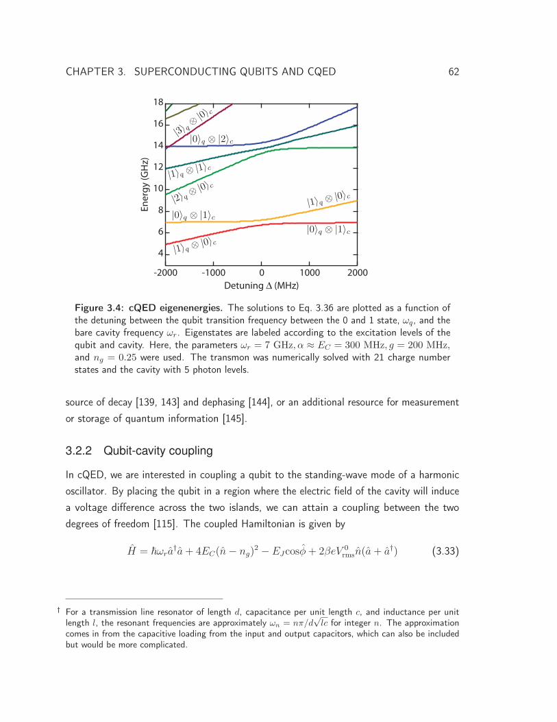
CHAPTER 3. SUPERCONDUCTING QUBITS AND CQED 62
18
16
14
12
10
8
6
4
Ener
gy (G
Hz)
-2000 -1000 0 1000 2000Detuning (MHz)
|1〉q ⊗ |0〉c
|0〉q ⊗ |1〉c|2〉q ⊗
|0〉c|1〉q ⊗ |1〉c
|0〉q ⊗ |2〉c|3〉q⊗ |0〉c
|1〉q ⊗ |0〉c
|0〉q ⊗ |1〉c
Figure 3.4: cQED eigenenergies. The solutions to Eq. 3.36 are plotted as a function ofthe detuning between the qubit transition frequency between the 0 and 1 state, ωq, and thebare cavity frequency ωr. Eigenstates are labeled according to the excitation levels of thequbit and cavity. Here, the parameters ωr = 7 GHz, α ≈ EC = 300 MHz, g = 200 MHz,and ng = 0.25 were used. The transmon was numerically solved with 21 charge numberstates and the cavity with 5 photon levels.
source of decay [139, 143] and dephasing [144], or an additional resource for measurementor storage of quantum information [145].
3.2.2 Qubit-cavity coupling
In cQED, we are interested in coupling a qubit to the standing-wave mode of a harmonicoscillator. By placing the qubit in a region where the electric field of the cavity will inducea voltage difference across the two islands, we can attain a coupling between the twodegrees of freedom [115]. The coupled Hamiltonian is given by
H = �ωra†a+ 4EC(n − ng)
2 − EJcosφ+ 2βeV 0rmsn(a+ a†) (3.33)
† For a transmission line resonator of length d, capacitance per unit length c, and inductance per unitlength l, the resonant frequencies are approximately ωn = nπ/d
√lc for integer n. The approximation
comes in from the capacitive loading from the input and output capacitors, which can also be includedbut would be more complicated.

CHAPTER 3. SUPERCONDUCTING QUBITS AND CQED 63
where ωr is the cavity frequency, β = Cg/CΣ the ratio of the effective capacitance Cg ofone side of the transmon to the cavity to total capacitance∗, and V 0
rms is the root-meansquared voltage at the qubit position per photon of the oscillator. We can re-write thisHamiltonian in the transmon basis |i〉 as
H = �ωra†a+ �
∑j
ωj|j〉〈j| + �∑i,j
gij|i〉〈j|(a+ a†) (3.34)
where the dipole coupling energies are
�gij = 2βeV 0rms〈i|n|j〉. (3.35)
The first term of Eq. 3.34 is the energy of the harmonic oscillator, the second the energy ofthe transmon, and the third a term that couples the two. This equation further simplifiesif we apply the rotating wave approximation (RWA), where we drop rapidly-rotating termsthat do not conserve energy (for example, terms that promote the energy of both thetransmon and the photon), giving
H = �ωra†a+ �
∑j
ωj|j〉〈j| +(�∑i
gi,i+1|i〉〈i| + 1|a† + h.c.
). (3.36)
We have plotted the solutions to this Hamiltonian as a function of qubit frequency inFig. 3.4.
In the limit of a small number of transmon levels, we can simplify this expressionby substituting the qubit with the anharmonic oscillator of Eq. 3.9. Labeling the cavitydegrees of freedom with the operator a and the qubit with b, we have
H = �ωra†a+ �ωq b
†b − α
2b†b†bb+ �g
(a†b+ ab†
). (3.37)
We can further simplify this by ignoring the higher levels entirely and, following Eq. 3.12,treat it like a spin. The result is the Jaynes-Cummings Hamiltonian
H = �ωr
(a†a+
1
2
)+
�ωq
2σz + �g
(a†σ− + aσ+
)(3.38)
∗ For the planar architecture, this gate capacitance Cg can be worked out by inverting a five by fivecapacitance network of the two islands of the transmon and the center pin and two ground planes of thecoplanar waveguide cavity. See, for example, Figure 2.8 in Lev Bishop’s 2010 thesis [113]. In the case ofthe 3D resonator, this geometric picture is no longer correct and it is necessary to numerically simulatethe impedances seen by the junctions.
CHAPTER 3. SUPERCONDUCTING QUBITS AND CQED 64
where g = g0,1, σ± is the raising and lowering operator of the spin, and where we haveagain included the vacuum energy of the harmonic oscillator for arbitrary reasons.
Studying these equations is arguably the goal of the remainder of this thesis, but we canimmediately highlight some physics by diagonalizing the Jaynes-Cummings Hamiltonian.Because of our simplifications, the Hamiltonian is a 2 by 2 block diagonal matrix, withdressed eigenstates
|n,+〉 = cos(θn)|n − 1, e〉 + sin(θn)|n, g〉|n,−〉 = − sin(θn)|n − 1, e〉 + cos(θn)|n, g〉
(3.39)
where tan(2θn) =2g
√n
Δ. This pair of states constitute the Jaynes-Cummings ladder and
parametrized by the total number of excitations ntot = a†a + σ+σ− > 0. Each pairconstitutes an excitation manifold∗, though for n = 0, we have only one state |0〉 = |0, g〉.The energies of these states are given by E0 = −�Δ
2and En,± = n�ωr ± �
2
√4g2n+Δ2
where Δ = ωq − ωr is the detuning between the qubit and cavity. When Δ = 0 and thequbit and cavity are in resonance, we are in the vacuum-Rabi regime, where the eigenstatesare symmetrically-weighted odd and even combinations of |n− 1, e〉 and |n, g〉. If you wereto prepare one of the undressed eigenstates at this point, the excitation would oscillatebetween the qubit and cavity at the rate g – a “vacuum-Rabi oscillation.”
3.2.3 Dispersive limit and qubit readout
We can further approximate the full transmon Hamiltonian (Eq. 3.38) in the dispersivelimit, where gj,j+1 � ωj+1,j − ωc. Using a unitary transformation [115], we can expand
∗ When talking about multiple-level transmon qubits, the number of states per excitation manifold growswith the excitation number. As we saw in Fig. 3.4, with only one excitation, we have (in the undressedbasis) only two states: |n = 1, q = 0〉 or |n = 0, q = 1〉. For two excitations, we now can have|n = 2, q = 0〉, |n = 1, q = 1〉, or |n = 0, q = 2〉, and so on. As you can imagine, with several multi-levelqubits at some reasonable level of excitation, the level diagram becomes very complicated (see, forexample, Fig. 8.5).
Incidentally, the reason that the Hamiltonian is block diagonal is that it commutes with the totalnumber of excitations Nex ≡ a†a+ 1+σz
2 . This structure gives this ladder of states. Each block is givenby
H(n+1)2x2 /� =
(nωc +
12ω01 g
√n+ 1
g√n+ 1 (n+ 1)ωc − 1
2ω01
).
CHAPTER 3. SUPERCONDUCTING QUBITS AND CQED 65
the Hamiltonian in powers of g/Δ, giving to second order [113]
H/� = ωra†a+
∑i
(ωi|i〉〈i| + χi,i+1|i+ 1〉〈i+ 1|)
− χ01a†a|0〉〈0| +
∞∑i=1
(χi−1,i − χi,i+1a
†a) |i〉〈i| (3.40)
where χij =g2ij
ωij−ωcare known as dispersive couplings. Here, the first term is again the
cavity and the second the transmon qubit energy. The third and fourth terms constitute arenormalization of the transmon and cavity energy levels due to their coupling; the fifthterm corresponds to the state-selective dispersive shifts. We can again take the two-levelapproximation of the qubit, giving the dispersive Jaynes-Cummings or number splittingHamiltonian
H = � (ω′c + χσz) a
†a+�
2ω′qσz. (3.41)
Here, both the qubit transition frequency ω′q = ω01+χ01 and the cavity transition frequency
ω′c = ωc − χ12/2 are renormalized by a quantity known as the Lamb shift. The dispersive
cavity shift χ = χ01 − χ12
2can be approximated for transmons as χ ≈ g2
ΔEC
�Δ−EC, with
Δ = ω01 − ωC .
Number splitting
Equation 3.41 deserves some analysis. We see that the term corresponding to the exchangeof excitations between the qubit and cavity is gone, replaced by the term χσza
†a. Thereare two ways of interpreting this term. First, we could group it with the qubit σz operator,giving Hlq = �σz
2
(ωq + 2χa†a
). The qubit frequency then depends on the number of
photons in the cavity. Explicitly, the qubit transition frequency will be ωq if the cavity isin its ground state, but ωq + 2χ if there is one photon, ωq + 4χ for two, and so on. Ifthere is a superposition of photon number states in the cavity (for example, if there isa coherent or thermal state), the qubit transition frequency will split into many peaks,a phenomenon known as number splitting [146]. When these peaks are resolved (in thestrong dispersive limit, discussed below), it is possible to perform number-selective pulseson the qubit, thus entangling the qubit with the number state of the cavity. This turns outto be extremely useful for a variety of quantum optics [92, 109] and quantum informationprocessing applications, as we will discuss in chapter 9.
CHAPTER 3. SUPERCONDUCTING QUBITS AND CQED 66
Qubit readout
Alternatively, we could group this extra term with the cavity number operator, giving usHc = � (ωc + χσz) a
†a. The cavity frequency now depends on the qubit state, moving 2χ
lower in frequency when the qubit is excited. For the case of transmon qubits, both theground and excited state peaks are moved up in frequency relative to the undressed cavityfrequency, but the ground state is shifted more, by what we call 2χ. Thus, in that case,ωc does not have physical significance and is instead a convenient frequency with which towrite the Hamiltonian. This dispersive shift is the mechanism that we will use to measurethe qubit: by measuring the frequency of the cavity, we can infer the state of the qubit.
Consider the situation where we pulse on a drive of strength εrf at some detuningδrf = ωRF − ωr from the bare cavity frequency. Ignoring any nonlinearity of the cavityitself, the resulting coherent state in the cavity will depend on the state of the qubit, andwill be given by [112, 147]
α± =εrf
κin+κout
2+ i(δrf ± χ)
(3.42)
where the subscript denotes the state of the qubit. This state has an amplitude
|α±|2 = n± =ε2rf
(κin+κout)2
4+ (δrf ± χ)2
. (3.43)
The amplitude inside the cavity is given by the product of the drive power with the inputcoupling strength, εrf = εin
√κin. We can detect these states by measuring the power
leaking out of the cavity in a transmission experiment. In the simple case where χ � κ,if we drive on resonance with the ground state cavity peak and get a relatively hightransmission, the qubit is in its ground state; if we get a relatively low transmission, thequbit is in its excited state. It is also possible to drive such that the amplitudes of α± arethe same, but the phase is different; which choice is optimal depends on system parameters.The distinguishability of these two states in either case is given by D = e−|α+−α−|2 , andcorresponds to the overlap of two gaussians on the complex plane. As we will see insection 6.1, optimizing this dispersive readout is a complicated task, especially whenaccounting for the nonlinearity that the cavity inherits from its qubit coupling.
The measurement operator corresponding to this operation is |0〉〈0|. What happensif more than one qubit is coupled to the single cavity? We can generalize the dispersive

CHAPTER 3. SUPERCONDUCTING QUBITS AND CQED 67
Hamiltonian as
H/� =
(ω′c +
∑i
χ(i)σ(i)z
)a†a+
1
2
∑i
ω(i)q σ(i)
z . (3.44)
The cavity frequency will then have a distinct frequency for each eigenstate of thecomputational state manifold. For example, with two qubits, the cavity will be found at ω′
c
for |00〉 but ω′c+χ(1) for |10〉, ω′
c+χ(2) for |01〉, and ω′c+χ(1)+χ(2) for |11〉. Then, if we
measure at ω′c and get a high transmission in the limit that the peaks are well-resolved, we
will have projected the system with the operator |00〉〈00|. For N qubits the measurementoperator can be understood to first order as |0⊗N〉〈0⊗N |. As we will see in section 7.3, itis somewhat more complicated when we include the fact that the cavity responses havefinite overlaps.
3.2.4 Single-qubit gates
The Jaynes-Cummings Hamiltonian is not the complete story: we must also include theeffect of a microwave drive. Conceptually, a drive can be understood as a coupled secondcavity mode that is displaced [113] and will leak energy into our primary cavity. We canapproximate its state in the limit that its displacement is large and coupling small as beingconstant and write
Hd = (a+ a†)(ξe−iωdt + ξ∗eiωdt
)= aξ∗eiωdt + a†ξe−iωdt (3.45)
where ξ is a parameter that defines the strength of the driving (given, in our toy model,by the product of the coupling times the displacement) and in the second part we haveapplied the rotating wave approximation (assuming ξ is much smaller than any relevanttransition frequency). We can add this term to equation 3.36, and by applying a unitarytransformation to go into the rotating frame of the drive, have
Hr/� = (ωr−ωd)a†a+
∑j
(ωj −jωd)|j〉〈j|+(∑
i
gi,i+1|i〉〈i+ 1|a† + h.c.
)+ aξ∗+ a†ξ.
(3.46)In this form the drive is acting on the cavity state, but we are interested in the dynamics
of the transmon. To see those instead, we can make another unitary transformation, the
CHAPTER 3. SUPERCONDUCTING QUBITS AND CQED 68
Glauber displacement transformation [113, 147], producing
H/� = Δra†a+
∑j
Δj|j〉〈j| +(∑
i
gi,i+1|i〉〈i+ 1|a† + |i+ 1〉〈i|a)
+1
2
∑j
(Ω∗R(t)|j〉〈j + 1| + ΩR(t)|j + 1〉〈j|)
(3.47)
where Δr = ωr − ωd, and Δj = ωj − jωd. ΩR(t) = 2gα(t) is the Rabi frequency of thedrive with α(t) the applied displacement as a function of time; we have ΩR = 2ξg/Δr forthe case of a time-independent drive. Taking the dispersive limit as we did in the previoussection, this further simplifies to
H/� = Δra†a+
∑j
Δj|j〉〈j| +∑j
χj,j+1|j + 1〉〈j + 1| − χ01a†a|0〉〈0|
+∑j=1
(χj−1,j − χj,j+1a†a)|j〉〈j|) + 1
2
∑j
(Ω∗R(t)|j〉〈j + 1| + ΩR(t)|j + 1〉〈j|).
(3.48)
Finally, treating the qubit as a two-level system, we arrive at the driven dispersive Jaynes-Cummings Hamiltonian
H =�
2Δqσz + �(Δr + χσz)a
†a+ �(Ω∗R(t)σ− + ΩR(t)σ+). (3.49)
Choosing ΩR(t) = ΩxR(t)cos(ωdt) + Ωy
R(t)sin(ωdt),
H =�
2Δqσz + �(Δr + χσz)a
†a+�
2(Ωx
R(t)σx + ΩyR(t)σy) (3.50)
and we see that by choosing the phase and amplitude of the drive, we can perform arbitraryrotations of our qubit about the x- and y-axes (defined in the rotating frame).
CHAPTER 3. SUPERCONDUCTING QUBITS AND CQED 69
3.2.5 Qubit-qubit coupling
We can generalize Eq. 3.40 to N transmons coupled to a single cavity by writing
H/� =N∑
n=1
{∑i
(ω(n)i |i〉n〈i|n + χ
(n)i,i+1|i+ 1〉n〈i+ 1|n
)− χ
(n)01 a
†a|0〉n〈0|n
+∞∑i=1
(χ(n)i−1,i − χ
(n)i,i+1a
†a)|i〉n〈i|n
+∑m>n
⎛⎝∑ij
g(n)j,j+1g
(m)i,i+1
(Δ
(n)j +Δ
(m)i
)2Δ
(n)j Δ
(m)i )
[|j〉n〈j + 1|n ⊗ |i+ 1〉m〈i|m+
+|j + 1〉n〈j|n ⊗ |i〉m〈i+ 1|m])}
+ ωra†a
(3.51)
where |i〉n denotes the ith level of the nth transmon, and the superscript (n) labels theparameters of the nth transmon. The first two lines are the sum of single transmonenergies and cavity couplings and the third and fourth lines control interactions betweentransmons and the cavity energy. This equation is a bit intimidating, so let us simplify tothe case of N = 2 and the two-level qubit approximation. Thus, equation 3.51 simplifiesto
H/� =(ωc + χ1σ
(1)z + χ2σ
(2)z
)a†a+
1
2ω1σ
(1)z +
1
2ω2σ
(2)z
+g1g2 (Δ1 +Δ2)
2Δ1Δ2
(σ(1)+ σ
(2)− + σ
(1)− σ
(2)+
).
(3.52)
We can identify these terms as, respectively, the cavity which may be dispersively shiftedby both qubits, the two bare qubit Hamiltonians, and a two-qubit swap interaction thatoccurs via a virtual interaction with the cavity. The direct qubit-qubit interaction strengthis known as J splitting∗, and could potentially be used to generate entanglement, as wewill discuss in section 7.2.1.
The full expression of equation 3.51 indicates that there will be interactions involvingthe higher excited states of transmons as well. We have found that the interaction of thecomputational state |11〉 with the non-computational state |02〉 is of particular experimental
∗ For more about this interaction, see section 4.3.2 of Jerry Chow’s 2010 thesis [114].

CHAPTER 3. SUPERCONDUCTING QUBITS AND CQED 70
relevance. As described in section 4.3.3 of Jerry Chow’s thesis [114], we can estimate thesize of this interaction with fourth-order perturbation theory and by approximating thetransmons as three-level systems [121]. Defining the parameter ξ as the magnitude of aneffective σ
(1)z ⊗ σ
(2)z interaction between the qubits, we have
ξ = −2g21g22
(1
δAΔ21
+1
δBΔ22
+1
Δ1Δ22
+1
Δ2Δ21
)(3.53)
where δA = ω(2)01 − ω
(1)12 , δB = ω
(1)01 − ω
(2)12 , and Δi = ω
(i)01 − ωr. This expression is only
valid when the 0 ↔ 1 transition of one qubit is far from the 1 ↔ 2 transition of the other,and it diverges when the transitions are in resonance. A full numerical diagonalizationof Eq. 3.51 accurately predicts the experimentally-measured ξ all the way through theavoided crossing [121]. This interaction is the basis of two different implementations of atwo-qubit entangling gate, one using the crossing off-resonantly and the other directly inresonance. We discuss both implementations in section 7.2.1 and section 7.2.2 respectively.Moreover, the virtual interaction of |102〉 and |003〉 in a three-qubit register is the basis ofa fast three-qubit gate we use to demonstrate quantum error correction, as we will discussin chapter 8.
3.2.6 Dissipation and the strong dispersive limit
So far we have not mentioned that these quantum objects are also coupled to theirenvironment and therefore suffer from dissipation. In the case of the cavity, we oftenexplicitly control this dissipation with the input and output RF coupling strengths becausewe want our measurement photons to be transmitted (see chapter 6). This will give thecavity a finite line width κ/2π, which is related to its lifetime by Tcav = 1/κ. (If we reduceour coupling enough, κ will no longer be dominated by our intentional coupling and insteadby, for example, photon absorption on the walls of the cavity.) The qubit also has a finitelifetime, parametrized by T1 = 1/γ. This is often set by either off-resonant decay throughthe cavity known as the “Purcell effect,” [139, 148] (section 6.2.1) or some uncontrolleddegree of freedom like lossy dielectric.
We define the strong dispersive limit as occurring when χ > γ, κ. There, the cavitywill move by more than a linewidth in response to a change of the qubit state, makingour measurement highly projective. More interestingly, in the case of photon number
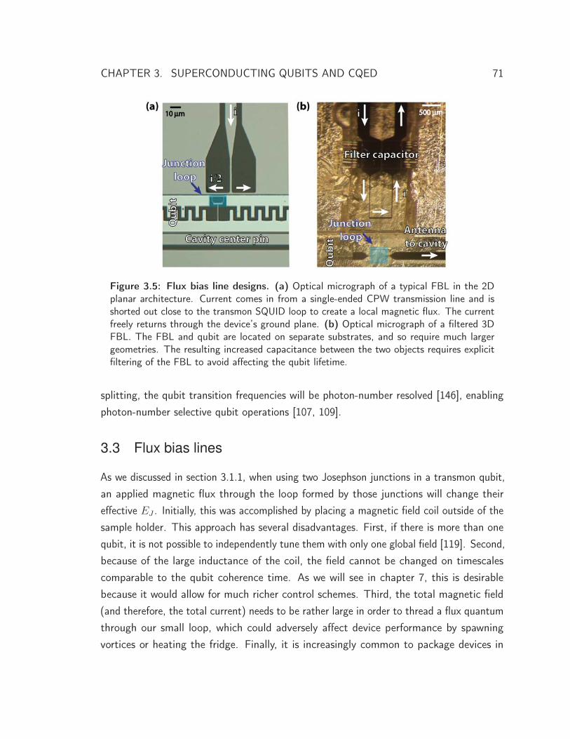
CHAPTER 3. SUPERCONDUCTING QUBITS AND CQED 71
Figure 3.5: Flux bias line designs. (a) Optical micrograph of a typical FBL in the 2Dplanar architecture. Current comes in from a single-ended CPW transmission line and isshorted out close to the transmon SQUID loop to create a local magnetic flux. The currentfreely returns through the device’s ground plane. (b) Optical micrograph of a filtered 3DFBL. The FBL and qubit are located on separate substrates, and so require much largergeometries. The resulting increased capacitance between the two objects requires explicitfiltering of the FBL to avoid affecting the qubit lifetime.
splitting, the qubit transition frequencies will be photon-number resolved [146], enablingphoton-number selective qubit operations [107, 109].
3.3 Flux bias lines
As we discussed in section 3.1.1, when using two Josephson junctions in a transmon qubit,an applied magnetic flux through the loop formed by those junctions will change theireffective EJ . Initially, this was accomplished by placing a magnetic field coil outside of thesample holder. This approach has several disadvantages. First, if there is more than onequbit, it is not possible to independently tune them with only one global field [119]. Second,because of the large inductance of the coil, the field cannot be changed on timescalescomparable to the qubit coherence time. As we will see in chapter 7, this is desirablebecause it would allow for much richer control schemes. Third, the total magnetic field(and therefore, the total current) needs to be rather large in order to thread a flux quantumthrough our small loop, which could adversely affect device performance by spawningvortices or heating the fridge. Finally, it is increasingly common to package devices in
CHAPTER 3. SUPERCONDUCTING QUBITS AND CQED 72
superconducting boxes (be it the sample holder or the 3D cavity itself), eliminating thepossibility of applying an external field because of the Meissner effect [149].
These issues prompted the development of flux bias lines or FBLs. Broadly speaking,FBLs are wires that get very close to the SQUID loop of a single qubit. Running currentthrough this wire will produce a magnetic field that changes the SQUID flux. To date, therehave been two implementations of these devices: one in the two-dimensional architecture[121], and much more recently, a second implementation that works for inline transmonqubits coupled to 3D cavities which we will introduced in section 4.2. As shown inFig. 3.5(a), the 2D FBL is implemented with a short-circuited transmission line thatis terminated near the loop. To place the maximum of current close to the loop, thetermination is off-center, and is symmetric about the center line in an attempt to controlthe impedance. The current returns in an uncontrolled way through the ground plane ofthe device. This simplifies things by requiring only one microwave port, though, as we willsee in section 7.1, it has the disadvantage of having finite DC flux coupling to other qubits.
The design of the 3D FBL is a bit different because the flux line and qubit are onseparate substrates, as shown in Fig. 3.5(b). As with the 2D case, a current-carrying wirecomes as close as possible to the qubit SQUID loop, but the size of the loop is significantlylarger as a result of the increased distance owing to being on different substrates. As wewill see below, it is necessary to add explicit filtering to these lines to prevent the qubitfrom decaying due to the substantial capacitance of this geometry. This FBL design alsohas two ports so the current flows along a well-defined path in and out of the sampleholder. As a result, there is zero measurable flux cross-coupling between qubits.
This section will focus primarily on the design considerations for extending FBLs tothe 3D architecture. Specifically, we wish to calculate whether it is possible to thread aflux quantum through the superconducting loop with a reasonable geometry and currentmagnitude. Initially, this was a major concern because the loop and FBL are so muchfarther apart than the 2D case and because of the flux screening of the Meissner effect.We will show that a flux quantum should be attainable using with an analytic calculation.We then discuss the consequence of the much larger geometry necessary: an increasedcapacitive coupling between the qubit and FBL leading to qubit relaxation. We calculatethat the qubit should decay in only a few microseconds due to this effect, but that it canbe eliminated with the addition of explicit low-pass filtering on the FBL.

CHAPTER 3. SUPERCONDUCTING QUBITS AND CQED 73
Figure 3.6: Flux bias line geometry. A current-carrying wire approaches a SQUID loopof width W and height H at a distance D away. The closest approach of the wire has alength L. The magnetic field of the wire coming to and from this length is cancelled out bysymmetry.
3.3.1 Flux coupling
One major question when designing the 3D FBLs was whether it would be possible tocouple a flux quantum into the SQUID loop without an excessive amount of current∗.Applying more than a few milliamps would constitute an unacceptable heat load on thefridge because of finite cable resistance. Following the work of Nissim Ofek and KevinChou (see appendix A), we can estimate the flux coupling analytically using the Biot-SavartLaw
B =
∫μ0I
4π
�dl × �r
|r|3 . (3.54)
The geometry in question is shown in Fig. 3.6, where we have a SQUID loop of width w
and height h positioned a distance d away from a wire of length L. The field at a position(x, y) due to the length of wire is given by
B(x, y) =μ0Iz
4π
∫ L/2
−L/2
y
((x − l)2 + y2)3/2dl
=μ0Iz
4πy
⎡⎣ L2− x√(
L2− x
)2+ y2
+L2+ x√(
L2+ x
)2+ y2
⎤⎦ .
(3.55)
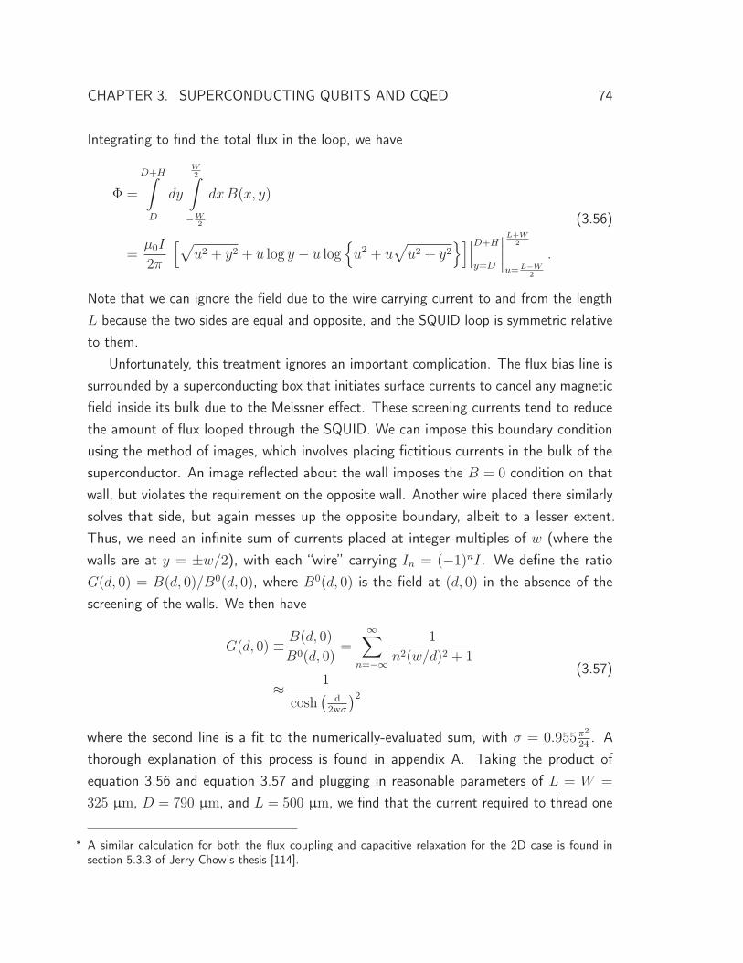
CHAPTER 3. SUPERCONDUCTING QUBITS AND CQED 74
Integrating to find the total flux in the loop, we have
Φ =
D+H∫D
dy
W2∫
−W2
dxB(x, y)
=μ0I
2π
[√u2 + y2 + u log y − u log
{u2 + u
√u2 + y2
}]∣∣∣D+H
y=D
∣∣∣∣L+W2
u=L−W2
.
(3.56)
Note that we can ignore the field due to the wire carrying current to and from the lengthL because the two sides are equal and opposite, and the SQUID loop is symmetric relativeto them.
Unfortunately, this treatment ignores an important complication. The flux bias line issurrounded by a superconducting box that initiates surface currents to cancel any magneticfield inside its bulk due to the Meissner effect. These screening currents tend to reducethe amount of flux looped through the SQUID. We can impose this boundary conditionusing the method of images, which involves placing fictitious currents in the bulk of thesuperconductor. An image reflected about the wall imposes the B = 0 condition on thatwall, but violates the requirement on the opposite wall. Another wire placed there similarlysolves that side, but again messes up the opposite boundary, albeit to a lesser extent.Thus, we need an infinite sum of currents placed at integer multiples of w (where thewalls are at y = ±w/2), with each “wire” carrying In = (−1)nI. We define the ratioG(d, 0) = B(d, 0)/B0(d, 0), where B0(d, 0) is the field at (d, 0) in the absence of thescreening of the walls. We then have
G(d, 0) ≡ B(d, 0)
B0(d, 0)=
∞∑n=−∞
1
n2(w/d)2 + 1
≈ 1
cosh(
d2wσ
)2 (3.57)
where the second line is a fit to the numerically-evaluated sum, with σ = 0.955π2
24. A
thorough explanation of this process is found in appendix A. Taking the product ofequation 3.56 and equation 3.57 and plugging in reasonable parameters of L = W =
325 μm, D = 790 μm, and L = 500 μm, we find that the current required to thread one
∗ A similar calculation for both the flux coupling and capacitive relaxation for the 2D case is found insection 5.3.3 of Jerry Chow’s thesis [114].
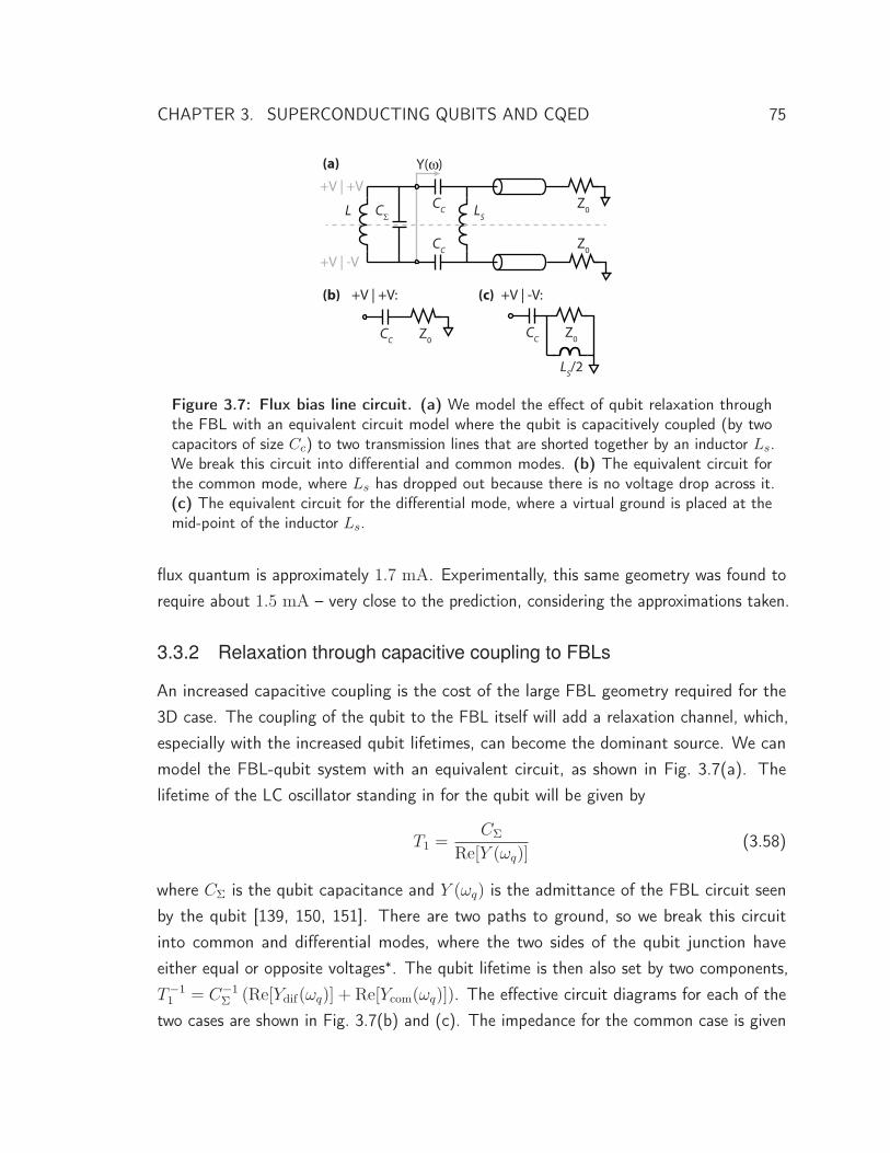
CHAPTER 3. SUPERCONDUCTING QUBITS AND CQED 75
L C CC
CC
LS
(a)
(b) (c)
Z0
Z0
CC Z0CC Z0
LS/2
Y( )+V | +V
+V | -V
+V | +V: +V | -V:
Figure 3.7: Flux bias line circuit. (a) We model the effect of qubit relaxation throughthe FBL with an equivalent circuit model where the qubit is capacitively coupled (by twocapacitors of size Cc) to two transmission lines that are shorted together by an inductor Ls.We break this circuit into differential and common modes. (b) The equivalent circuit forthe common mode, where Ls has dropped out because there is no voltage drop across it.(c) The equivalent circuit for the differential mode, where a virtual ground is placed at themid-point of the inductor Ls.
flux quantum is approximately 1.7 mA. Experimentally, this same geometry was found torequire about 1.5 mA – very close to the prediction, considering the approximations taken.
3.3.2 Relaxation through capacitive coupling to FBLs
An increased capacitive coupling is the cost of the large FBL geometry required for the3D case. The coupling of the qubit to the FBL itself will add a relaxation channel, which,especially with the increased qubit lifetimes, can become the dominant source. We canmodel the FBL-qubit system with an equivalent circuit, as shown in Fig. 3.7(a). Thelifetime of the LC oscillator standing in for the qubit will be given by
T1 =CΣ
Re[Y (ωq)](3.58)
where CΣ is the qubit capacitance and Y (ωq) is the admittance of the FBL circuit seenby the qubit [139, 150, 151]. There are two paths to ground, so we break this circuitinto common and differential modes, where the two sides of the qubit junction haveeither equal or opposite voltages∗. The qubit lifetime is then also set by two components,T−11 = C−1
Σ (Re[Ydif(ωq)] + Re[Ycom(ωq)]). The effective circuit diagrams for each of thetwo cases are shown in Fig. 3.7(b) and (c). The impedance for the common case is given
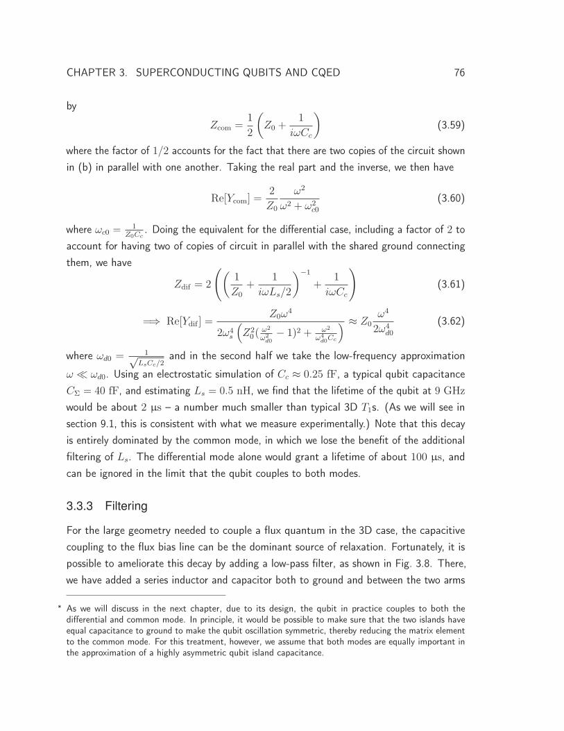
CHAPTER 3. SUPERCONDUCTING QUBITS AND CQED 76
by
Zcom =1
2
(Z0 +
1
iωCc
)(3.59)
where the factor of 1/2 accounts for the fact that there are two copies of the circuit shownin (b) in parallel with one another. Taking the real part and the inverse, we then have
Re[Ycom] =2
Z0
ω2
ω2 + ω2c0
(3.60)
where ωc0 =1
Z0Cc. Doing the equivalent for the differential case, including a factor of 2 to
account for having two of copies of circuit in parallel with the shared ground connectingthem, we have
Zdif = 2
((1
Z0
+1
iωLs/2
)−1
+1
iωCc
)(3.61)
=⇒ Re[Ydif ] =Z0ω
4
2ω4s
(Z2
0(ω2
ω2d0
− 1)2 + ω2
ω4d0Cc
) ≈ Z0ω4
2ω4d0
(3.62)
where ωd0 = 1√LsCc/2
and in the second half we take the low-frequency approximation
ω � ωd0. Using an electrostatic simulation of Cc ≈ 0.25 fF, a typical qubit capacitanceCΣ = 40 fF, and estimating Ls = 0.5 nH, we find that the lifetime of the qubit at 9 GHz
would be about 2 μs – a number much smaller than typical 3D T1s. (As we will see insection 9.1, this is consistent with what we measure experimentally.) Note that this decayis entirely dominated by the common mode, in which we lose the benefit of the additionalfiltering of Ls. The differential mode alone would grant a lifetime of about 100 μs, andcan be ignored in the limit that the qubit couples to both modes.
3.3.3 Filtering
For the large geometry needed to couple a flux quantum in the 3D case, the capacitivecoupling to the flux bias line can be the dominant source of relaxation. Fortunately, it ispossible to ameliorate this decay by adding a low-pass filter, as shown in Fig. 3.8. There,we have added a series inductor and capacitor both to ground and between the two arms
∗ As we will discuss in the next chapter, due to its design, the qubit in practice couples to both thedifferential and common mode. In principle, it would be possible to make sure that the two islands haveequal capacitance to ground to make the qubit oscillation symmetric, thereby reducing the matrix elementto the common mode. For this treatment, however, we assume that both modes are equally important inthe approximation of a highly asymmetric qubit island capacitance.
CHAPTER 3. SUPERCONDUCTING QUBITS AND CQED 77
L CCC
CC
LSZ0
Z0
Cg
Cg
CS
Lf
Lf
(a)
+V | +V
+V | -V
Y( )
(b) +V | +V:Cg
LfZ0
(c) +V | -V:
Lf
2Cs
CC
LS/2
CC
Cg
Z0
Figure 3.8: Filtered flux bias line circuit. (a) In order to reduce qubit relaxation viacapacitive coupling to the outside world, we add a low-pass filter to the FBL. We are free todo this because the FBL control signals are always below 1 GHz while the qubit transitionfrequencies are typically 5− 10 GHz. The filter is implemented with a series inductor andparallel capacitor, and again can be split into common and differential modes, shown in (b)and (c).
of the bias line. We can again calculate the impedance for the common and differentialmodes of this structure, with
Zcom =1
2
((1
Z0
+ iωCg
)−1
+ iωLf +1
iωCc
)(3.63)
Zdif = 2
⎛⎝(( 1
Z0
+ iω (Cg + 2Cs)
)−1
+ iωLf
)−1
+1
iωLs/2
⎞⎠−1
+2
iωCc
. (3.64)
As before, inverting these equations and taking their real part gives us the expectedqubit lifetime using Eq. 3.58. The largest geometric inductance that can be madeon this scale without being affected by self-resonances is about Lmax
f ≈ 1 nH. Thus,the job of filtering comes down to the capacitance. Experimentally, it is possible toget a large capacitance by using a three-layer lithography process, where Cg can beas large as tens of pF. Evaluating Eq. 3.63 and Eq. 3.64 with reasonable parameters(Cc = 0.25 fF, CΣ = 40 fF, Ls = 0.5 nH, Cg = 10 pF, Lf = 1 nH), and assuming Cs = 0
since it is much smaller than Cg, we predict a common mode lifetime of ∼ 1.6 ms and
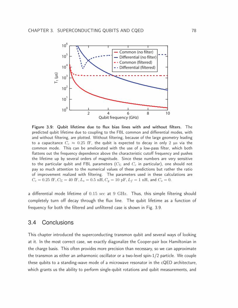
CHAPTER 3. SUPERCONDUCTING QUBITS AND CQED 78
100
101
102
103
104
105
106
T 1 (μ
s)
108642Qubit frequency (GHz)
Common (no filter) Differential (no filter) Common (filtered) Differential (filtered)
Figure 3.9: Qubit lifetime due to flux bias lines with and without filters. Thepredicted qubit lifetime due to coupling to the FBL common and differential modes, withand without filtering, are plotted. Without filtering, because of the large geometry leadingto a capacitance Cc ≈ 0.25 fF, the qubit is expected to decay in only 2 μs via thecommon mode. This can be ameliorated with the use of a low-pass filter, which bothflattens out the frequency dependence above the characteristic cutoff frequency and pushesthe lifetime up by several orders of magnitude. Since these numbers are very sensitiveto the particular qubit and FBL parameters (CΣ and Cc in particular), one should notpay so much attention to the numerical values of these predictions but rather the ratioof improvement realized with filtering. The parameters used in these calculations areCc = 0.25 fF, CΣ = 40 fF, Ls = 0.5 nH, Cg = 10 pF, Lf = 1 nH, and Cs = 0.
a differential mode lifetime of 0.15 sec at 9 GHz. Thus, this simple filtering shouldcompletely turn off decay through the flux line. The qubit lifetime as a function offrequency for both the filtered and unfiltered case is shown in Fig. 3.9.
3.4 Conclusions
This chapter introduced the superconducting transmon qubit and several ways of lookingat it. In the most correct case, we exactly diagonalize the Cooper-pair box Hamiltonian inthe charge basis. This often provides more precision than necessary, so we can approximatethe transmon as either an anharmonic oscillator or a two-level spin-1/2 particle. We couplethese qubits to a standing-wave mode of a microwave resonator in the cQED architecture,which grants us the ability to perform single-qubit rotations and qubit measurements, and

CHAPTER 3. SUPERCONDUCTING QUBITS AND CQED 79
mediates couplings between qubits that will be used to generate entanglement. The termsresponsible for these properties are found in the Jaynes-Cummings Hamiltonian, thoughsome work is required to convert them into a transparent form. We use flux bias lines tocontrol the frequency of qubits in-situ, and recently extended them to the 3D architecture.There, the geometry required to couple a flux quantum results in a substantial capacitancebetween the FBL and qubit and therefore a new channel for qubit decay that can dominatefor typical parameters. We have the capacity to to eliminate this channel with the additionof a low-pass filter to the FBL. In the next chapter, we will explain the actual experimentalrealization of both planar and tunable 3D cQED.

CHAPTER 4
Experimental Design and Setup
Now that we have a solid theoretical background in both quantum information processingand superconducting qubits, we can shift our attention to the experiment. This
chapter begins by introducing the planar cQED architecture [106, 118] which has been theprimary focus of the Schoelkopf lab for many years. It uses a coplanar waveguide geometrythat is entirely specified with optical lithography. We will introduce the basic features ofthis geometry and conclude with how such devices are fabricated and packaged.
More recently, our lab has shifted to a new architecture that replaces the CPWcavity with a three-dimensional superconducting box [62]. This change has realized hugeimprovements in qubit coherence, though it initially came the a cost of reduced control.We seek to re-introduce the ability to tune the qubits using flux without giving up thelifetime gains of the 3D transmon. This motivation sets the stage to introduce the tunable3D cQED architecture, which integrates flux tunability by utilizing a vertical transmonwhose Josephson junction is located in the bulk aluminum rather than inside the cavityitself. We can therefore access the junction with a wire placed on a separate piece ofsapphire. We will first introduce the design principles of the tunable architecture and showhow it is assembled. We next explain the design of the cavity, sample box, qubits, and fluxbias lines.
We then discuss more broadly the experimental details of measuring any cQED device.
81

CHAPTER 4. EXPERIMENTAL DESIGN AND SETUP 82
Cin Cout
l
ah
t
b
top view side view
substrate
Figure 4.1: Coplanar waveguide geometry. (top) The planar cavity is implemented witha coplanar waveguide terminated with two capacitors. The length between these capacitorssets the resonance frequency of the cavity, and the size of the capacitors determines itscoupling Qc. (side) The waveguide is patterned on top of a sapphire substrate with thicknessh ≈ 420 μm. The width a of the CPW is typically 10 μm, with a spacing from the groundplane b = 4.2 μm. The thickness of the niobium film t = 200 nm. These parameters willgive an impedance Z ≈ 50 Ω.
We use a helium dilution fridge to cool the device to ∼ 20 mK. The cables going into andout of the fridge must be thoroughly filtered, with attenuation on the incoming lines andcirculators on the outgoing ones. We then examine a typical wiring diagram used bothto generate control pulses and measure a cQED device, and explain common areas forvariants and recent improvements. We conclude with a description of how mixers can beused to implement pulse modulation much more cheaply than using a full vector generator,but how doing so requires a series of calibrations.
4.1 Planar design
The planar or “2D” geometry used in most of the experiments presented in this thesishas been developed for several years, beginning with the first realization of cQED withCooper-pair boxes in 2004 [118]. Other than the transition to transmon qubits and theintroduction of flux bias lines, the overall geometry has not changed significantly in theyears since. Therefore, instead of introducing all the details of the architecture which havebeen thoroughly discussed in previous papers [118, 119, 121] and theses [112, 114, 152],we will instead summarize the features of planar cQED.
The resonators in planar cQED are implemented with a coplanar waveguide (CPW)geometry, as shown in Fig. 4.1. The length of the center pin between two capacitors setsthe frequency of the resonator and the magnitude of those capacitances sets the coupling
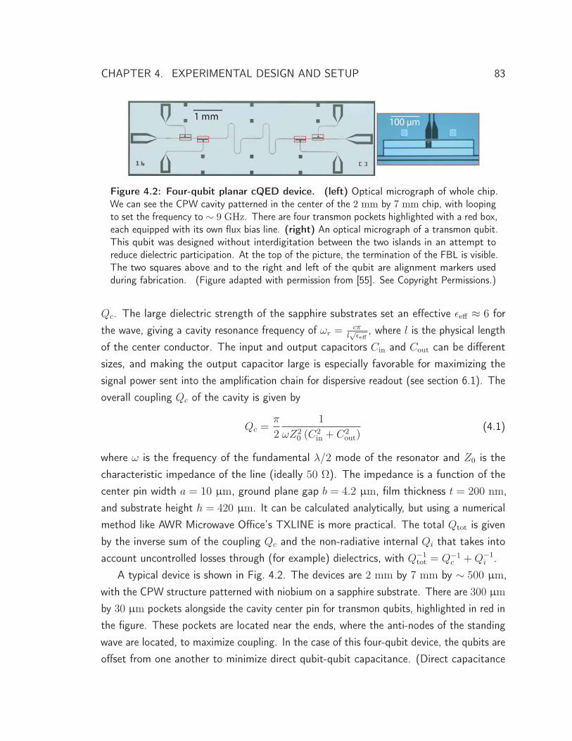
CHAPTER 4. EXPERIMENTAL DESIGN AND SETUP 83
Figure 4.2: Four-qubit planar cQED device. (left) Optical micrograph of whole chip.We can see the CPW cavity patterned in the center of the 2 mm by 7 mm chip, with loopingto set the frequency to ∼ 9 GHz. There are four transmon pockets highlighted with a red box,each equipped with its own flux bias line. (right) An optical micrograph of a transmon qubit.This qubit was designed without interdigitation between the two islands in an attempt toreduce dielectric participation. At the top of the picture, the termination of the FBL is visible.The two squares above and to the right and left of the qubit are alignment markers usedduring fabrication. (Figure adapted with permission from [55]. See Copyright Permissions.)
Qc. The large dielectric strength of the sapphire substrates set an effective εeff ≈ 6 forthe wave, giving a cavity resonance frequency of ωr =
cπl√εeff
, where l is the physical lengthof the center conductor. The input and output capacitors Cin and Cout can be differentsizes, and making the output capacitor large is especially favorable for maximizing thesignal power sent into the amplification chain for dispersive readout (see section 6.1). Theoverall coupling Qc of the cavity is given by
Qc =π
2
1
ωZ20 (C
2in + C2
out)(4.1)
where ω is the frequency of the fundamental λ/2 mode of the resonator and Z0 is thecharacteristic impedance of the line (ideally 50 Ω). The impedance is a function of thecenter pin width a = 10 μm, ground plane gap b = 4.2 μm, film thickness t = 200 nm,and substrate height h = 420 μm. It can be calculated analytically, but using a numericalmethod like AWR Microwave Office’s TXLINE is more practical. The total Qtot is givenby the inverse sum of the coupling Qc and the non-radiative internal Qi that takes intoaccount uncontrolled losses through (for example) dielectrics, with Q−1
tot = Q−1c +Q−1
i .A typical device is shown in Fig. 4.2. The devices are 2 mm by 7 mm by ∼ 500 μm,
with the CPW structure patterned with niobium on a sapphire substrate. There are 300 μm
by 30 μm pockets alongside the cavity center pin for transmon qubits, highlighted in red inthe figure. These pockets are located near the ends, where the anti-nodes of the standingwave are located, to maximize coupling. In the case of this four-qubit device, the qubits areoffset from one another to minimize direct qubit-qubit capacitance. (Direct capacitance
CHAPTER 4. EXPERIMENTAL DESIGN AND SETUP 84
would add an undesirable constant ZZ interaction between the qubits.) These devicesemploy flux bias lines that are similarly implemented with 50 Ω CPW but short-circuitednear the location of the transmon SQUID as described in section 3.3. The figure showsthat each of the transmon pockets is equipped with a FBL, making this a six-port devicewhen the input and output cavity ports are counted. On the right, a zoom-in of one of thetransmon qubits is shown. Engineering the parameters EC and β of the transmon qubitrequires inverting a 5 by 5 capacitance matrix (see Ref. 115). However, to first order, βcan be controlled with the long dimension of the qubit (closest to the center pin) and EC
with spacing between the two islands. In this picture, the end of the FBL is visible, alignedso that one of the two current paths is centered on the transmon SQUID loop.
4.1.1 Planar fabrication
All planar resonators in this thesis were produced by a similar process [105]. It beginswith sputtering a ∼ 200 nm thick niobium film on 2-inch C-plane corundum (α − Al2O3)wafer using a d.c.-magnetron. This wafer is covered with S1808 photoresist, on which theresonator structures are patterned with contact UV optical lithography. The niobium is dryetched with a fluorine-based reactive ion etcher, followed by lift-off in acetone. The waferis diced into 2 mm x 7 mm chips. To create the qubits, each individual chip is coveredwith two additional layers of photoresist (top 100 nm of 950K PMMA A3, bottom 550 nmMMA(8.5)-MAA EL13 copolymer) and patterned with electron-beam lithography. Thebottom layer is more sensitive to electrons than the top, giving a natural ∼ 80 nm undercutwhich eases lift-off. After development, aluminum is deposited with a double-angle electronbeam evaporation to create the Al−AlOx −Al Josephson junctions and qubit capacitors,with a 15% O2 15 torr 12-minute oxidation step between subsequent depositions. Finally,the undeveloped photoresist is removed with lift-off, leaving behind only the aluminumthat was defined by electron lithography. Junction resistances (which are related to Emax
J )can be tested by either fabricating explicit test junctions alongside the qubits or by directlyprobing the transmon islands. As long as appropriate precautions are taken to limit thetest current and prevent static shocks, this measurement does not appear to harm thejunction.
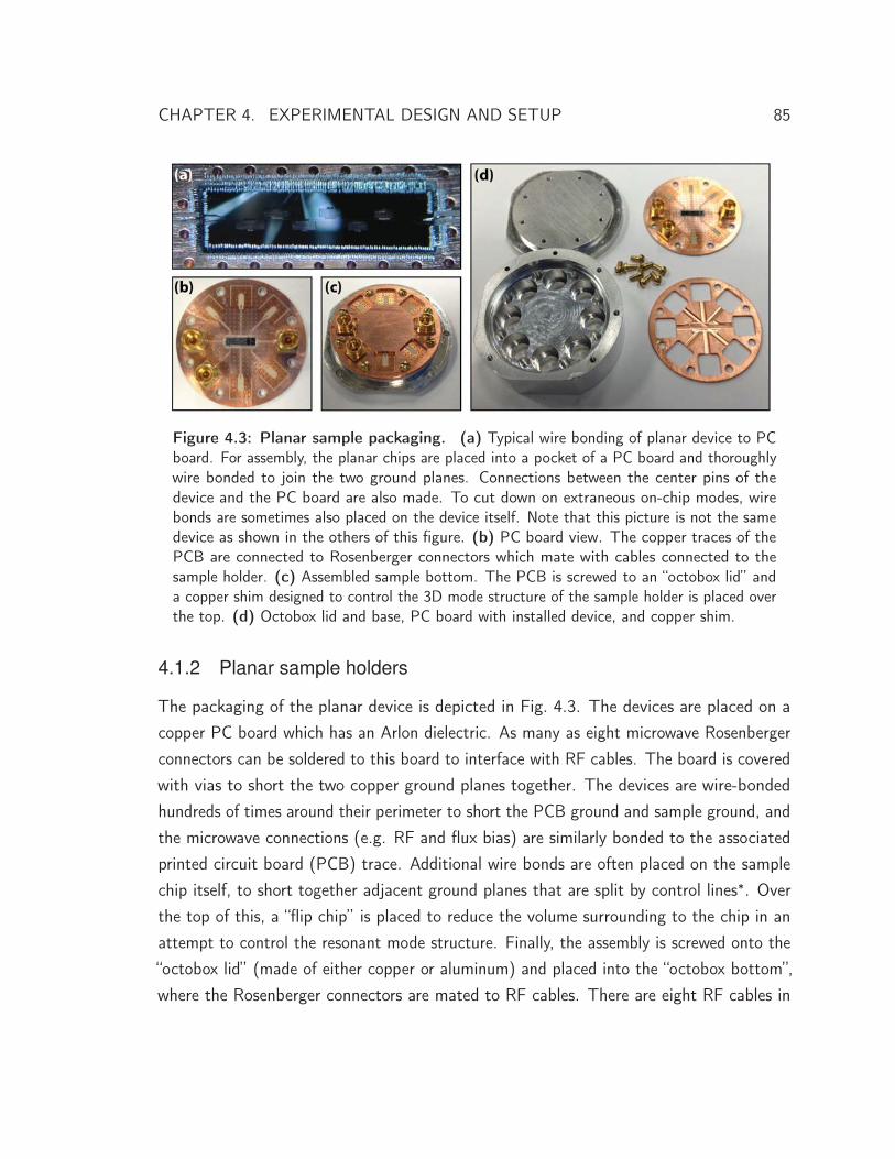
CHAPTER 4. EXPERIMENTAL DESIGN AND SETUP 85
Figure 4.3: Planar sample packaging. (a) Typical wire bonding of planar device to PCboard. For assembly, the planar chips are placed into a pocket of a PC board and thoroughlywire bonded to join the two ground planes. Connections between the center pins of thedevice and the PC board are also made. To cut down on extraneous on-chip modes, wirebonds are sometimes also placed on the device itself. Note that this picture is not the samedevice as shown in the others of this figure. (b) PC board view. The copper traces of thePCB are connected to Rosenberger connectors which mate with cables connected to thesample holder. (c) Assembled sample bottom. The PCB is screwed to an “octobox lid” anda copper shim designed to control the 3D mode structure of the sample holder is placed overthe top. (d) Octobox lid and base, PC board with installed device, and copper shim.
4.1.2 Planar sample holders
The packaging of the planar device is depicted in Fig. 4.3. The devices are placed on acopper PC board which has an Arlon dielectric. As many as eight microwave Rosenbergerconnectors can be soldered to this board to interface with RF cables. The board is coveredwith vias to short the two copper ground planes together. The devices are wire-bondedhundreds of times around their perimeter to short the PCB ground and sample ground, andthe microwave connections (e.g. RF and flux bias) are similarly bonded to the associatedprinted circuit board (PCB) trace. Additional wire bonds are often placed on the samplechip itself, to short together adjacent ground planes that are split by control lines∗. Overthe top of this, a “flip chip” is placed to reduce the volume surrounding to the chip in anattempt to control the resonant mode structure. Finally, the assembly is screwed onto the“octobox lid” (made of either copper or aluminum) and placed into the “octobox bottom”,where the Rosenberger connectors are mated to RF cables. There are eight RF cables in
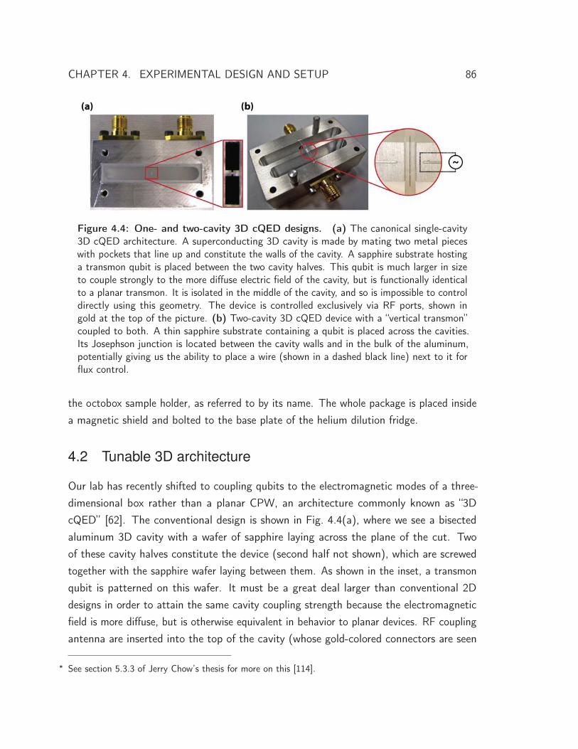
CHAPTER 4. EXPERIMENTAL DESIGN AND SETUP 86
Figure 4.4: One- and two-cavity 3D cQED designs. (a) The canonical single-cavity3D cQED architecture. A superconducting 3D cavity is made by mating two metal pieceswith pockets that line up and constitute the walls of the cavity. A sapphire substrate hostinga transmon qubit is placed between the two cavity halves. This qubit is much larger in sizeto couple strongly to the more diffuse electric field of the cavity, but is functionally identicalto a planar transmon. It is isolated in the middle of the cavity, and so is impossible to controldirectly using this geometry. The device is controlled exclusively via RF ports, shown ingold at the top of the picture. (b) Two-cavity 3D cQED device with a “vertical transmon”coupled to both. A thin sapphire substrate containing a qubit is placed across the cavities.Its Josephson junction is located between the cavity walls and in the bulk of the aluminum,potentially giving us the ability to place a wire (shown in a dashed black line) next to it forflux control.
the octobox sample holder, as referred to by its name. The whole package is placed insidea magnetic shield and bolted to the base plate of the helium dilution fridge.
4.2 Tunable 3D architecture
Our lab has recently shifted to coupling qubits to the electromagnetic modes of a three-dimensional box rather than a planar CPW, an architecture commonly known as “3DcQED” [62]. The conventional design is shown in Fig. 4.4(a), where we see a bisectedaluminum 3D cavity with a wafer of sapphire laying across the plane of the cut. Twoof these cavity halves constitute the device (second half not shown), which are screwedtogether with the sapphire wafer laying between them. As shown in the inset, a transmonqubit is patterned on this wafer. It must be a great deal larger than conventional 2Ddesigns in order to attain the same cavity coupling strength because the electromagneticfield is more diffuse, but is otherwise equivalent in behavior to planar devices. RF couplingantenna are inserted into the top of the cavity (whose gold-colored connectors are seen
∗ See section 5.3.3 of Jerry Chow’s thesis for more on this [114].
CHAPTER 4. EXPERIMENTAL DESIGN AND SETUP 87
at the top of the picture), and are also functionally identical to the RF drive ports ofthe planar devices. (See Adam Sears’s thesis [153] for a more detailed description of thegeometry of these devices.)
This 3D architecture has realized huge gains in coherence time, with measured T1 andT2 in excess of 100 μs. The reason for this nearly two orders of magnitude improvementis thought to be primarily due to reduced energy storage in lossy materials [154–157],though quasiparticle dynamics may also play a role [158–161]. The dielectric quality ofsurfaces and interfaces of materials are suspected to be of poor quality compared to thebulk. Relatively small features like those found in the planar architecture tend to focus alarge fraction of stored energy near these surfaces, while large features will have a smallerparticipation ratio in that lossy material because the field lines will penetrate deeper intothe bulk. Thus, instead of attempting to improve the material properties as many believedwas required, the 3D architecture bypasses the issue by reducing the qubit’s susceptibilityto the problem. In the process of studying these qubits, it also became clear that properthermalization and filtering was crucial to getting good performance and is responsible foranother factor of two in coherence [144, 162].
These improvements come at some cost. The qubit is suspended in the middle of asuperconducting cavity, greatly limiting our ability to have direct control of it. We cannot,for example, run wires for flux bias to the qubit nor interface these wires through the wallof the cavity without modifying the mode structure (and, likely the lifetime) of the cavity.Since the cavity is typically superconducting, threading external flux is also not a possibility.(We could instead use a copper cavity [64], but the cavity quality factor will be much lower,requiring a much larger qubit-cavity detuning to limit Purcell relaxation.) Is this a significantdisadvantage? Though flux bias lines are extensively used in this thesis for the purposeof entangling gates, that is unlikely to be their most important application∗. However,fast tunability would play a critical role in demonstrations of hardware-efficient quantumerror correction [93], entanglement distillation between distant pairs of qubits [163–165],and distribution of quantum information between subsystems [166]. The coupling ofa qubit to the cavity bus could be modulated to control the inherited nonlinearity andthe dispersive shift of the oscillator in real time, useful for continuous-variable quantuminformation processing [92, 93, 167]. Controlling the interactions between individual qubits,particularly those coupled to more than one cavity, could be used to shuttle quantuminformation between distant subsystems. Fine-tuning system parameters would ease theimplementation of schemes that have strict parameter requirements [168]. Individual QND

CHAPTER 4. EXPERIMENTAL DESIGN AND SETUP 88
qubit readout, reset, or drives also requires individual qubit addressability, and are crucialfor quantum error correction and are some of the DiVincenzo criteria [79] enumerated insection 2.2.2.
The capacity to address individual qubits is a desirable capability, but we would like toregain it without sacrificing the improvements of 3D cQED. Fortunately, work on couplinga single 3D qubit to two different cavities [107] has suggested a solution. As shown inFig. 4.4(b), a “vertical transmon” can be laid across two cavities, with antennas stickinginto both, and yielding strong coupling∗. (This has also been done previously in the planararchitecture, as reported in Ref. 109.) As a result, the Josephson junction of the qubit islocated between these two cavities in the bulk of the aluminum and it is no longer isolated.We could potentially thread in a current-carrying wire from the side to apply magnetic flux,as shown by the dashed lines on the right of (b). This is the principle concept behind thetunable 3D cQED architecture. In this section, we first show how the tunable architectureis assembled which will give a broad overview of the design principles. We then introducethe specific design of the tunable cavities themselves, the two versions of the verticaltransmon qubits, and the flux bias lines.
4.2.1 Tunable 3D cQED assembly
To implement the idea inspired by the two-cavity 3D device for the tunable 3D architecture,we place flux bias control wires adjacent to the vertical transmon qubits in the bulk ofthe cavity material. Both single-cavity and two-cavity variants of the architecture exist.As shown in Fig. 4.5(a), the single-cavity device has pockets for as many as four tunablevertical transmon qubits. Adjacent to each pocket are trenches for flux bias lines that arepatterned on separate slivers of sapphire and abut against the qubit at the location of itsjunction (middle inset). The slivers protrude from the side of the cavity and are received bytwo copper PC boards attached to the sample holder surrounding the cavity (right inset).In a manner identical to the planar devices, these FBLs are wire-bonded to copper traces
∗ Recently, an all-RF entangling gate which requires no qubit tunability has been demonstrated [169]. Thequbits used in that experiment were single-junction devices and not susceptible to flux noise, thereforeenjoying longer T2 times.
∗ The vertical transmon is actually a middle-ground between the full 3D qubit shown Fig. 4.4(a) and theplanar geometry in the sense that its participation in surfaces is somewhat higher than the 3D geometry.Though other differences may be responsible, this increased participation could be the reason that verticaltransmons thus far seem to be limited to T1 ≈ 20− 40 μs. So, for now at least, we have compromisedsome coherence for improved control.

CHAPTER 4. EXPERIMENTAL DESIGN AND SETUP 89
Figure 4.5: Single-cavity tunable 3D architecture assembly. (a) As described in thebody of the text, the tunable 3D architecture employs vertical transmons located in trenchestraversing the cavity that are coupled via antenna that stick in. These qubits are controlledwith separately fabricated flux bias lines, which are able to access the qubit SQUID loopbecause it is located in the bulk of the material. The FBLs attach to conventional PC boardslocated outside the cavity, on a sample holder that surrounds it. (b) Assembly diagram ofthe four components of the architect, showing the “3D octobox” sample holder in copper(though it most commonly made of aluminum), inside which the cavity is placed. (c) Pictureof a fully-assembled device, showing the eight cables that can be used to control flux bias.(d) Picture of a coaxial RF coupler used to address the cavity, inserted through a hole in thebottom of the sample holder and into the cavity.
that are themselves soldered to a Rosenberger connector. The qubits and the flux biaslines are held in place by flattening indium metal around them at several locations. This isshown in the right inset for the case of the flux bias line and in the middle inset for thequbit (the latter case is more difficult to see due to the low contrast between aluminumand indium). For additional shielding and to better connect the two cavity halves, indiumwire can also be placed around the cavity in a rounded-rectangular groove.
The architecture is assembled in four main sections, as shown in Fig. 4.5(b). Thecavity is placed in the pocket of a sample holder box (copper-colored in the figure) and issecured with three screws. To the sides of the cavity are placed the copper PC boards,which are similarly screwed to the sample holder. In this configuration, the qubits andflux bias lines can be inserted and secured with indium, the FBLs wirebonded, and theindium seal placed. The second half of the cavity is placed over the top, which must becarefully aligned by scrutinizing the matching flux bias line trenches on the top, and issecured with four more screws. Finally, the sample holder lid which mates the PC board

CHAPTER 4. EXPERIMENTAL DESIGN AND SETUP 90
Figure 4.6: Two-cavity 3D octobox assembly. The two-cavity version of the tunable 3Darchitecture can support as many as five tunable qubits, with a pair of qubits coupled to eachcavity and a fifth qubit coupled to both. It is compatible with the single-cavity sample holder,and so its assembly is essentially identical. Here, a variant of the architecture is shown thatmerges the bottom cavity with the bottom of the sample holder in an attempt to cut downon RF crosstalk of the couplers via the small gap between the cavity and sample holder thatotherwise arises.
connectors to conventional cables is placed over the top and screwed to the bottom part.Since this lid has eight flux bias line ports, it is known as a “3D octobox.” A picture of afully-assembled device is shown in Fig. 4.5(c), where the eight cables have been installed.RF cavity control is achieved in a similar way as with conventional 3D cQED, with anRF coaxial cable sticking into the side of the cavity through a corresponding hole in theoctobox. As shown in Fig. 4.5(d), the coupler soldered to a copper bar that is used forthermalization, shorting of ground planes, and securing it to the octobox.
The two-cavity version of the tunable architecture is shown in Fig. 4.6. It is designedand assembled much like the single-cavity version. The primary difference is that thedifferent locations for the qubits and flux bias lines require a distinct PC board design.Each cavity supports two local tunable qubits, with a fifth tunable qubit located betweenthe two cavities in the same geometry as the original two-cavity vertical transmon. Thereis room for two RF couplers on either side of the octobox, enabling full RF control of bothcavities. Since the octobox has only four ports on either side, two of the flux bias lines onthe side with the fifth qubit’s FBL are shorted to the PC board instead of returning theircurrent through a cable. The two-cavity device also omits the indium trench for lack ofspace.
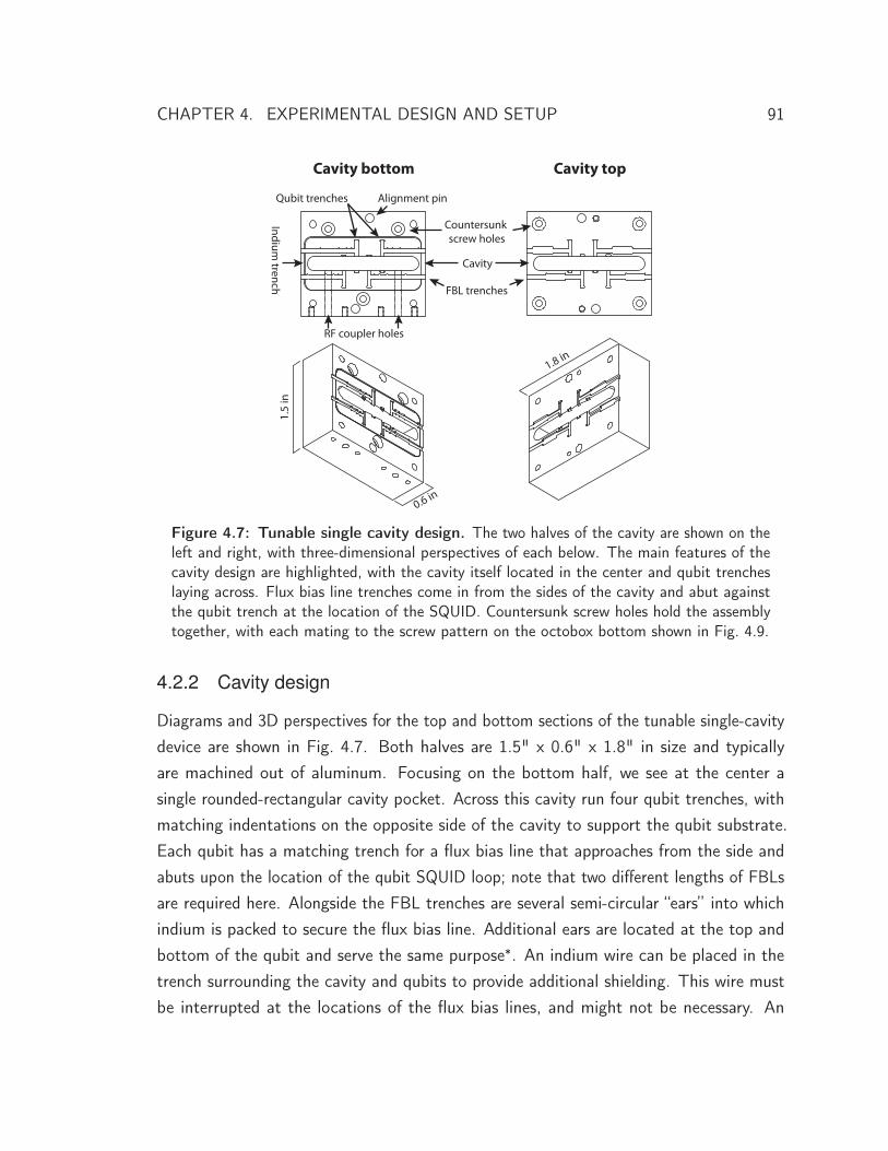
CHAPTER 4. EXPERIMENTAL DESIGN AND SETUP 91
FBL trenches
Indium trench
RF coupler holes
Qubit trenches
Cavity
Alignment pin
Countersunk screw holes
Cavity bottom Cavity top
1.5
in
0.6 in
1.8 in
Figure 4.7: Tunable single cavity design. The two halves of the cavity are shown on theleft and right, with three-dimensional perspectives of each below. The main features of thecavity design are highlighted, with the cavity itself located in the center and qubit trencheslaying across. Flux bias line trenches come in from the sides of the cavity and abut againstthe qubit trench at the location of the SQUID. Countersunk screw holes hold the assemblytogether, with each mating to the screw pattern on the octobox bottom shown in Fig. 4.9.
4.2.2 Cavity design
Diagrams and 3D perspectives for the top and bottom sections of the tunable single-cavitydevice are shown in Fig. 4.7. Both halves are 1.5" x 0.6" x 1.8" in size and typicallyare machined out of aluminum. Focusing on the bottom half, we see at the center asingle rounded-rectangular cavity pocket. Across this cavity run four qubit trenches, withmatching indentations on the opposite side of the cavity to support the qubit substrate.Each qubit has a matching trench for a flux bias line that approaches from the side andabuts upon the location of the qubit SQUID loop; note that two different lengths of FBLsare required here. Alongside the FBL trenches are several semi-circular “ears” into whichindium is packed to secure the flux bias line. Additional ears are located at the top andbottom of the qubit and serve the same purpose∗. An indium wire can be placed in thetrench surrounding the cavity and qubits to provide additional shielding. This wire mustbe interrupted at the locations of the flux bias lines, and might not be necessary. An

CHAPTER 4. EXPERIMENTAL DESIGN AND SETUP 92
alignment pin similar to the one shown in Fig. 4.4(b) can also ease assembly. There arethree countersunk screw holes used to attach the cavity to the octobox sample holder;due to the countersinking, the head of the screw is below the cavity plane and does notinterfere with assembly. There are four clear holes on the corners of the device, throughwhich we inserted the screws securing the top cavity. Finally, there are two holes drilledfrom the outer wall of the device to the cavity for RF coupling (dashed lines). Adjacent toboth holes are tapped holes to which the RF couplers are fastened.
The top of the cavity is designed in much the same way. There is a matching rounded-rectangular cavity pocket and matching trenches for the qubit and flux bias lines. Thosebias line trenches flare out to make room for wirebonding of the flux bias line filters tothe body of the cavity. Without the extra room, the wirebonds would be sheared off bythe wall of the trench during assembly. There are four countersunk screw holes to holdthe cavity together, with the countersinking on the back side surface (not shown in theperspective view). Finally, next to the alignment pin holes are tapped screw holes that maybe used to separate the two cavities in a controlled manner if they become stuck together.
We show the two-cavity device in Fig. 4.8. There, we see two cavities of slightlydifferent size (with unloaded bare cavity frequencies of about 7.8 GHz and 9.2 GHz).Both the top and bottom cavities have qubit trenches traversing them, positioned at thesame location as the single-cavity devices so that the same flux bias lines can be recycled.A fifth tunable qubit is located between the two cavities at the exact center. The FBL andqubit trenches also have the “ears” used to secure their contents with indium. There arefour RF coupling holes with matching tapped screw holes for two cavities. Countersunkscrew holes are located at the top and bottom of the devices, used for assembly, though thebottom device has two screws rather than three due to lack of space. For the same reason,the indium seal trench has been omitted. There are also alignment pins and correspondingtapped screw holes on the top of the device to ease assembly and disassembly.
4.2.3 Octobox design
A diagram of the 3D octobox sample holder is shown in Fig. 4.9. As before, we showseparate diagrams for the top and bottom of the device, each with 3D perspective views
∗ In addition to making it possible to machine. Since this trench will be milled out with a circular tool, ifwe did not have these ears, the edges of the trench would be rounded and a rectangular substrate wouldnot fit.
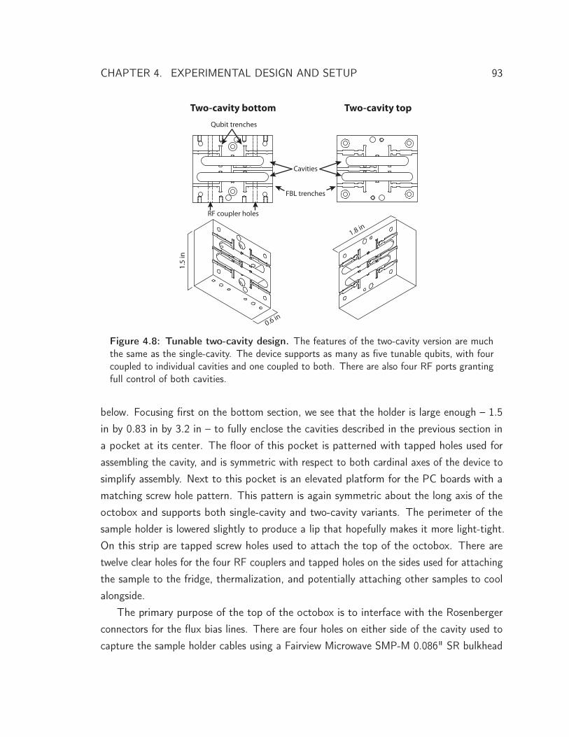
CHAPTER 4. EXPERIMENTAL DESIGN AND SETUP 93
FBL trenches
RF coupler holes
Qubit trenches
Cavities
Two-cavity bottom Two-cavity top
1.5
in
0.6 in
1.8 in
Figure 4.8: Tunable two-cavity design. The features of the two-cavity version are muchthe same as the single-cavity. The device supports as many as five tunable qubits, with fourcoupled to individual cavities and one coupled to both. There are also four RF ports grantingfull control of both cavities.
below. Focusing first on the bottom section, we see that the holder is large enough – 1.5in by 0.83 in by 3.2 in – to fully enclose the cavities described in the previous section ina pocket at its center. The floor of this pocket is patterned with tapped holes used forassembling the cavity, and is symmetric with respect to both cardinal axes of the device tosimplify assembly. Next to this pocket is an elevated platform for the PC boards with amatching screw hole pattern. This pattern is again symmetric about the long axis of theoctobox and supports both single-cavity and two-cavity variants. The perimeter of thesample holder is lowered slightly to produce a lip that hopefully makes it more light-tight.On this strip are tapped screw holes used to attach the top of the octobox. There aretwelve clear holes for the four RF couplers and tapped holes on the sides used for attachingthe sample to the fridge, thermalization, and potentially attaching other samples to coolalongside.
The primary purpose of the top of the octobox is to interface with the Rosenbergerconnectors for the flux bias lines. There are four holes on either side of the cavity used tocapture the sample holder cables using a Fairview Microwave SMP-M 0.086" SR bulkhead
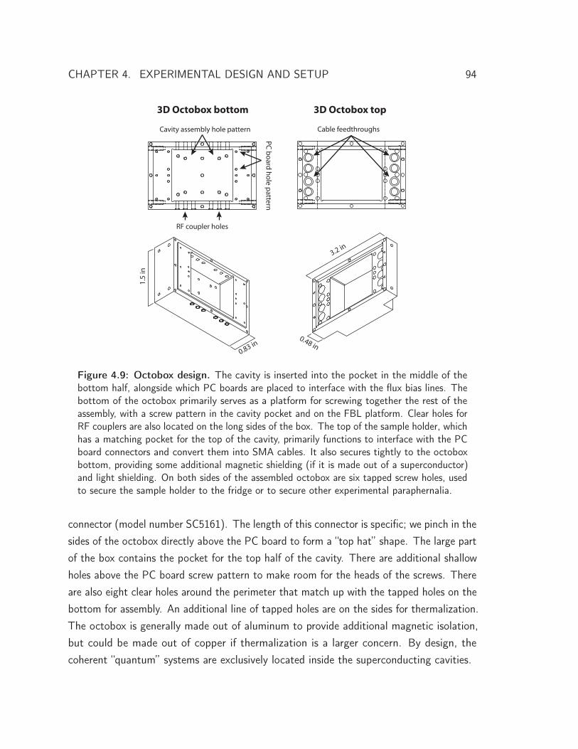
CHAPTER 4. EXPERIMENTAL DESIGN AND SETUP 94
RF coupler holes
3D Octobox bottom 3D Octobox top
1.5
in
0.83 in
3.2 in
Cavity assembly hole pattern
PC board hole pattern
Cable feedthroughs
0.48 in
Figure 4.9: Octobox design. The cavity is inserted into the pocket in the middle of thebottom half, alongside which PC boards are placed to interface with the flux bias lines. Thebottom of the octobox primarily serves as a platform for screwing together the rest of theassembly, with a screw pattern in the cavity pocket and on the FBL platform. Clear holes forRF couplers are also located on the long sides of the box. The top of the sample holder, whichhas a matching pocket for the top of the cavity, primarily functions to interface with the PCboard connectors and convert them into SMA cables. It also secures tightly to the octoboxbottom, providing some additional magnetic shielding (if it is made out of a superconductor)and light shielding. On both sides of the assembled octobox are six tapped screw holes, usedto secure the sample holder to the fridge or to secure other experimental paraphernalia.
connector (model number SC5161). The length of this connector is specific; we pinch in thesides of the octobox directly above the PC board to form a “top hat” shape. The large partof the box contains the pocket for the top half of the cavity. There are additional shallowholes above the PC board screw pattern to make room for the heads of the screws. Thereare also eight clear holes around the perimeter that match up with the tapped holes on thebottom for assembly. An additional line of tapped holes are on the sides for thermalization.The octobox is generally made out of aluminum to provide additional magnetic isolation,but could be made out of copper if thermalization is a larger concern. By design, thecoherent “quantum” systems are exclusively located inside the superconducting cavities.
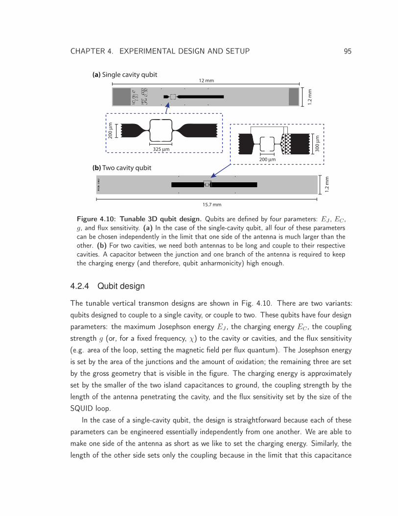
CHAPTER 4. EXPERIMENTAL DESIGN AND SETUP 95
12 mm
1.2
mm
15.7 mm
1.2
mm
325 m
200
m
(a) Single cavity qubit
(b) Two cavity qubit
300
m
200 m
Figure 4.10: Tunable 3D qubit design. Qubits are defined by four parameters: EJ , EC ,g, and flux sensitivity. (a) In the case of the single-cavity qubit, all four of these parameterscan be chosen independently in the limit that one side of the antenna is much larger than theother. (b) For two cavities, we need both antennas to be long and couple to their respectivecavities. A capacitor between the junction and one branch of the antenna is required to keepthe charging energy (and therefore, qubit anharmonicity) high enough.
4.2.4 Qubit design
The tunable vertical transmon designs are shown in Fig. 4.10. There are two variants:qubits designed to couple to a single cavity, or couple to two. These qubits have four designparameters: the maximum Josephson energy EJ , the charging energy EC , the couplingstrength g (or, for a fixed frequency, χ) to the cavity or cavities, and the flux sensitivity(e.g. area of the loop, setting the magnetic field per flux quantum). The Josephson energyis set by the area of the junctions and the amount of oxidation; the remaining three are setby the gross geometry that is visible in the figure. The charging energy is approximatelyset by the smaller of the two island capacitances to ground, the coupling strength by thelength of the antenna penetrating the cavity, and the flux sensitivity set by the size of theSQUID loop.
In the case of a single-cavity qubit, the design is straightforward because each of theseparameters can be engineered essentially independently from one another. We are able tomake one side of the antenna as short as we like to set the charging energy. Similarly, thelength of the other side sets only the coupling because in the limit that this capacitance

CHAPTER 4. EXPERIMENTAL DESIGN AND SETUP 96
is much larger than the other side, the smaller one drops out∗. The flux loop size isalso mostly irrelevant to both parameters and can be changed without redesigning theentire qubit. Thus, as we shown in Fig. 4.10(a), we can see that the left antenna ismuch smaller than the right, which sticks into the cavity by approximately 1.5 mm. (Thelocation of the rightmost pair of arrows on the qubit denotes the wall of the cavity whenit is installed.) Though we have this design freedom, quantitatively predicting the qubitparameters requires numerical simulation of the geometry using a program like AnsoftHFSS. This qubit also demonstrates an unusual feature: silver pads bookending the 12mm by 1.2 mm sapphire substrate. When shorted to the cavity with indium wire, this wasintended to better thermalize the qubit and act as a quasiparticle drain.
Since we need both antennas to strongly couple to both cavities, we do not have thefreedom of making one side of the qubit tiny for a two-cavity device. In the first two-cavity3D cQED device [107], this trick was still viable given the possibility of spacing the cavitiesmore closely (only 2 mm apart), placing the junction off-center, and making the antennavery thin. In the case of the tunable architecture, however, we must have the cavities atleast 4 mm apart to fit the flux bias line and require that the SQUID loop is near the centerso that we can couple sufficient flux (see Fig. 4.6). In order to circumvent this problem,we add a new sophistication: a capacitor that couples one side of the qubit island to itsantenna. As seen in the inset of (b), there is a very short piece of metal on the right sideadjacent to a long antenna. The holes surrounding the capacitive gap between these twofeatures are present for technical reasons: to help avoid overdosing during electron beamlithography and shorting out the capacitor as a result. The size of this capacitor and thelength of the antenna then sets the size of the coupling to the right cavity and the positionof the gap relative to the SQUID loop sets the charging energy. We are free to choosethe length of the opposite antenna to address other concerns. The wires connecting thetwo sides of the junction and the auxiliary antenna are there to prevent the junctions fromgetting destroyed by static discharge during dicing, and are removed prior to installation.Comparing the two qubit designs, we also see that the SQUID loop in the case of thesingle-cavity device is a great deal larger than the two-cavity device. This is due to the
∗ A corollary of this is when the two island capacitances are very different, the mode of the transmon isquite asymmetric as well. It will therefore couple to both the common and differential modes of a fluxbias line. We calculated in section 3.3.2 that the contribution to T1 of the common mode dominatesthat of the differential mode, which is unfortunate, since that is exactly the component we become moresensitive to as we utilize this trick. One way to solve that problem is to use filtering, as we have done,but it may have been unnecessary if we were more clever about qubit design.
CHAPTER 4. EXPERIMENTAL DESIGN AND SETUP 97
fact that the single-cavity qubit was designed first, when we were not yet confident in ourability to thread flux. As it became clear that flux coupling was not a problem, we choseto reduce the size of the loop in an attempt to reduce the magnitude of flux noise. Wealso increased the pitch size of the antenna from 200 μm to 300 μm to reduce surfaceparticipation.
4.2.5 Flux bias line design
The flux bias lines used in the tunable 3D architecture are on their own 1.5 mm by∼ 20 mm sapphire substrates. The simplest form of these, shown in Fig. 4.11(a), is awire that passes from one of the PCB ports to the other, coming as close as possible tothe qubit SQUID to maximize coupling. As explained in section 3.3.2, however, this typeof bias line design is unacceptable because it will shorten the lifetime of the qubit viacapacitive coupling. The solution to this problem is to add a low-pass filter (section 3.3.3)to the line in the form of an inductor and capacitor. In Fig. 4.11(b-c), we show twoversions of this filter. In both cases, the inductance of the low-pass filter is produced by alength of wire 1 mm long, corresponding to approximately 1 nH. It is not possible to getsubstantially more than this from a wire at this frequency without running into problemsof self-resonances. As a result, the two bias line designs differ only in their capacitorimplementation.
The first-generation filter design, shown in Fig. 4.11(b), uses an interdigitated capacitor.The center pin of the FBL fans out with numerous fingers, which are interleaved withfingers of metal islands above and below the line. There are also fingers between thetwo lines, granting extra capacitance to the differential mode. During operation, theislands on the top and bottom are shorted to the electrical ground of the cavity usingeither compressed indium or wire bonds. This filter helps somewhat by increasing themeasured T1 by approximately a factor of four. It cannot, however, provide sufficientcapacitance to solve the problem. The surface length of the fingers sets the frequencyscale of self-resonance; adding more fingers to get more capacitance would push thisself-resonance frequency down, violating the lumped-element approximation, and makingit inoperable as a capacitor at the relevant frequencies. We knew this would be the caseprior to measuring it, however, and only tested it because the fabrication was no morecomplicated than the unfiltered FBL found in (a). We also enlarged the width of thetransmission line used for the filtered FBLs to attempt a better impedance match.
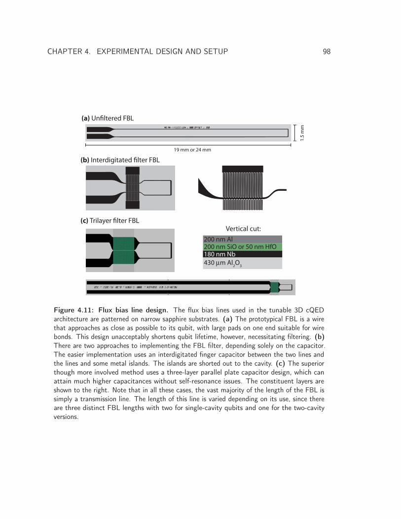
CHAPTER 4. EXPERIMENTAL DESIGN AND SETUP 98
(a) Unfiltered FBL
(b) Interdigitated filter FBL
(c) Trilayer filter FBL
19 mm or 24 mm
1.5
mm
200 nm Al200 nm SiO or 50 nm HfO180 nm Nb430 m Al2O3
Vertical cut:
Figure 4.11: Flux bias line design. The flux bias lines used in the tunable 3D cQEDarchitecture are patterned on narrow sapphire substrates. (a) The prototypical FBL is a wirethat approaches as close as possible to its qubit, with large pads on one end suitable for wirebonds. This design unacceptably shortens qubit lifetime, however, necessitating filtering. (b)There are two approaches to implementing the FBL filter, depending solely on the capacitor.The easier implementation uses an interdigitated finger capacitor between the two lines andthe lines and some metal islands. The islands are shorted out to the cavity. (c) The superiorthough more involved method uses a three-layer parallel plate capacitor design, which canattain much higher capacitances without self-resonance issues. The constituent layers areshown to the right. Note that in all these cases, the vast majority of the length of the FBL issimply a transmission line. The length of this line is varied depending on its use, since thereare three distinct FBL lengths with two for single-cavity qubits and one for the two-cavityversions.
CHAPTER 4. EXPERIMENTAL DESIGN AND SETUP 99
A superior filter is shown in Fig. 4.11(c), which uses a three-layer lithography process.Instead of relying on the capacitance between two pieces of metal on the same plane (whichis extremely inefficient) this approach uses the third dimension to produce a canonicalparallel plate capacitor with a dielectric in between. The lithography is straightforward:first, as shown in black in (c), the flux bias line is patterned in niobium. It flares outconsiderably at the point where we wish to have our capacitor. Next, a thin layer ofdielectric – we have tried 200 nm of silicon monoxide or 50 nm of hafnium oxide – isdeposited in the area designated in green. Finally, a 200 nm thick strip of aluminum isdeposited over the whole thing (denoted in gray), which constitutes the other side of thecapacitor. The aluminum is shorted to the bulk of the cavity with wire bonds. (This typeof filter is shown in both Fig. 4.5 and Fig. 4.6.) This approach has the advantage ofgetting a capacitance many times higher before being concerned about self-resonances. Inpractice, it seems to eliminate any relaxation through the FBL (section 9.1).
4.3 Dilution fridges and wiring diagram
Most of the experiments detailed in this thesis were performed in a Cryoconcept “wet”helium dilution refrigerator. The fridge uses a bath of liquid helium to get to 4 Kelvinand a standard closed-circuit 3He-4He dilution unit to attain its base temperature ofTb ∼ 10 − 15 mK. The advertised cooling power at 100 mK is 200 μW. The heliumbath must be filled approximately twice a week with 50 L of liquid. The level of this bathconstantly changes, as does the fridge temperature profile, causing the attenuation of thecables to drift slightly in time. More recently, the lab has shifted toward using OxfordInstruments brand “dry” fridges that use a high-performance pulse tube to reach 4 K.These have the advantage of being much cheaper to run as they do not require liquidhelium. This provides both more experimental space and less overall bulk; it also requiresmuch less work to cool (due to e.g. the lack of need for an indium seal) and operate.Given the rapidly increasing price of helium in the context of these advantages, it is likelythat many cryogenic labs will shift toward these dry fridges if experimentally possible∗.
The wiring diagram used to produce GHZ states, as described in chapter 7, is shownin Fig. 4.12 and is representative of all the experiments. Let us first explain what happensinside the fridge, as denoted by the dashed blue box. Thermal Johnson noise coming down
∗ One example of where this is unfeasible is for experiments that are extremely sensitive to vibration.
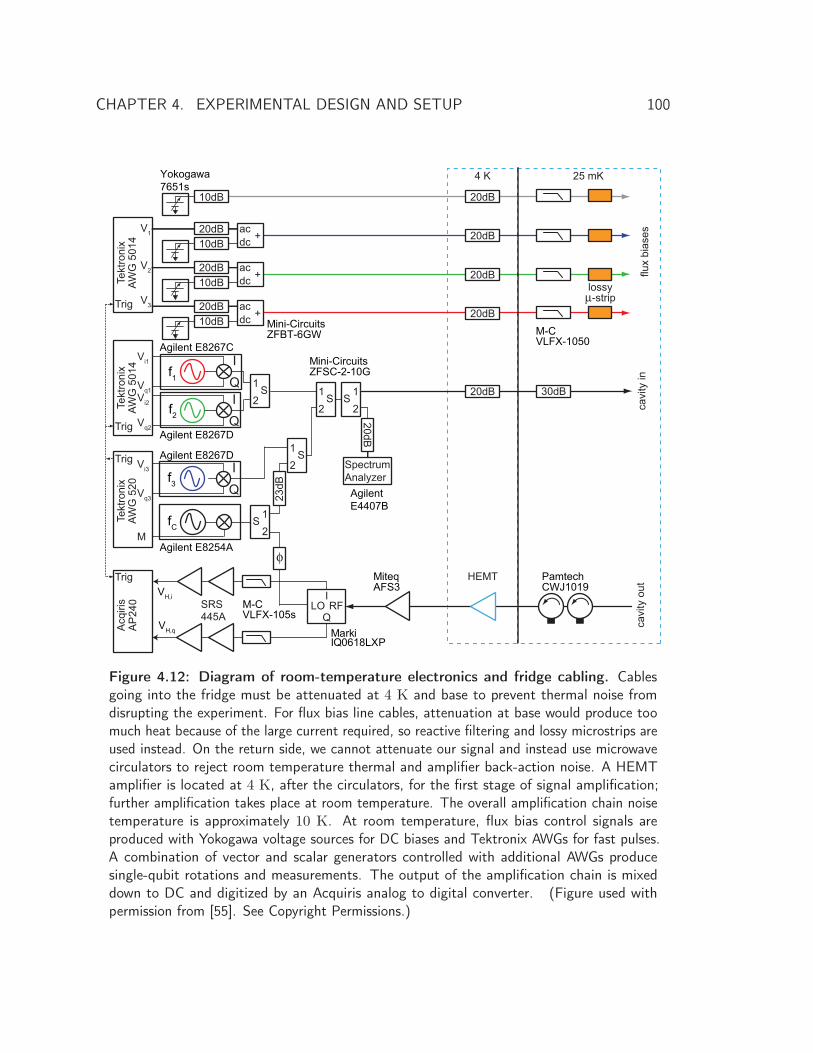
CHAPTER 4. EXPERIMENTAL DESIGN AND SETUP 100
Figure 4.12: Diagram of room-temperature electronics and fridge cabling. Cablesgoing into the fridge must be attenuated at 4 K and base to prevent thermal noise fromdisrupting the experiment. For flux bias line cables, attenuation at base would produce toomuch heat because of the large current required, so reactive filtering and lossy microstrips areused instead. On the return side, we cannot attenuate our signal and instead use microwavecirculators to reject room temperature thermal and amplifier back-action noise. A HEMTamplifier is located at 4 K, after the circulators, for the first stage of signal amplification;further amplification takes place at room temperature. The overall amplification chain noisetemperature is approximately 10 K. At room temperature, flux bias control signals areproduced with Yokogawa voltage sources for DC biases and Tektronix AWGs for fast pulses.A combination of vector and scalar generators controlled with additional AWGs producesingle-qubit rotations and measurements. The output of the amplification chain is mixeddown to DC and digitized by an Acquiris analog to digital converter. (Figure used withpermission from [55]. See Copyright Permissions.)
CHAPTER 4. EXPERIMENTAL DESIGN AND SETUP 101
cables would constitute an unacceptable noise source to the sample, and must be “filtered”by lowering its effective temperature via cold attenuation. In the low effective-temperaturelimit, voltage noise is linear in temperature SV (ω) ≈ 4kbTR, so we can attenuate at acold stage by a factor α = Thot/Tcold. Thus, cables carrying signals into the fridge areattenuated by 20 dB at 4 Kelvin to cut down room temperature 290 K noise. The RFdrive line used for measurement and single-qubit rotations (black) is further attenuated by30 dB to go from 4 K to base. The lossy stainless steel cables themselves (which are usedfor their minimal thermal conduction) constitute an additional 10 dB of attenuation, for atotal of ∼ 80 dB. Since resistively attenuating the large DC currents used for flux biaswould generate too much heat at base, the flux bias line cables (gray, blue, green, red) usereactive low-pass and lossy strip-line filters. They reject Johnson noise as well as preventerroneous qubit coupling, while maintaining a 50 Ω impedance match at low frequency.
On the amplification (output) side, we do not have the luxury of attenuating our smallsignals, and instead use microwave circulators. Circulators are three-port non-reciprocaldevices by which microwaves going into one port are transmitted only to the port to theright [170, 171]. Waves going to port 1 would come out port 2, those going into port 2would go to port 3, and into 3, out 1. We terminate one of these ports with a matched 50 Ω
load to absorb the noise coming down from room temperature, but the signal coming upfrom the sample is transmitted. This effective two-port device is also known as an isolatorand can be purchased by itself. Reverse-isolation is not perfect, so we typically use two ormore in series. In addition to rejecting noise from room temperature, circulators also blockthe back-action noise produced by the high electron mobility transistor (HEMT) amplifier.This amplifier has about 40 dB of gain and a noise temperature of 5 K. If we include cablelosses and reflections between the device and the amplifier, the total amplification chainnoise temperature is closer to 10 K. We use additional room temperature amplification aswell, bringing the total output gain to ∼ 70 dB.
Outside of the fridge, there are three sets of equipment. Starting from the top ofFig. 4.12, we have the four flux bias line channels. This wiring diagram is for a cQEDsample with four flux-tunable qubits. In the GHZ experiment described in chapter 7, onlythree of these qubits were used and the fourth tuned far away and left in its ground state.The first FBL channel (in gray) provides a quiescent DC bias for this unused qubit, whichneeds no fast control. It is attenuated at room temperature by 10 dB to reduce the noisecoming from the Yokogawa 7651s voltage source. The remaining three flux channels (inblue, green, and red) have a Yokogawa voltage source to provide DC offsets, but are also
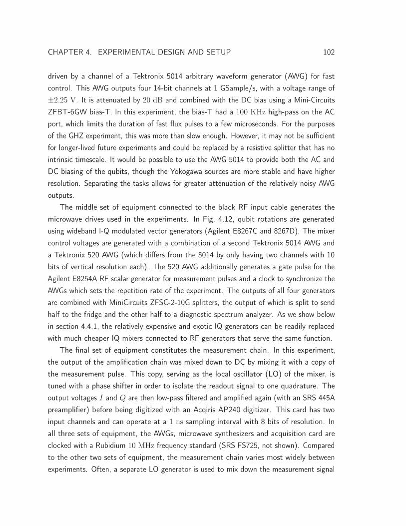
CHAPTER 4. EXPERIMENTAL DESIGN AND SETUP 102
driven by a channel of a Tektronix 5014 arbitrary waveform generator (AWG) for fastcontrol. This AWG outputs four 14-bit channels at 1 GSample/s, with a voltage range of±2.25 V. It is attenuated by 20 dB and combined with the DC bias using a Mini-CircuitsZFBT-6GW bias-T. In this experiment, the bias-T had a 100 KHz high-pass on the ACport, which limits the duration of fast flux pulses to a few microseconds. For the purposesof the GHZ experiment, this was more than slow enough. However, it may not be sufficientfor longer-lived future experiments and could be replaced by a resistive splitter that has nointrinsic timescale. It would be possible to use the AWG 5014 to provide both the AC andDC biasing of the qubits, though the Yokogawa sources are more stable and have higherresolution. Separating the tasks allows for greater attenuation of the relatively noisy AWGoutputs.
The middle set of equipment connected to the black RF input cable generates themicrowave drives used in the experiments. In Fig. 4.12, qubit rotations are generatedusing wideband I-Q modulated vector generators (Agilent E8267C and 8267D). The mixercontrol voltages are generated with a combination of a second Tektronix 5014 AWG anda Tektronix 520 AWG (which differs from the 5014 by only having two channels with 10bits of vertical resolution each). The 520 AWG additionally generates a gate pulse for theAgilent E8254A RF scalar generator for measurement pulses and a clock to synchronize theAWGs which sets the repetition rate of the experiment. The outputs of all four generatorsare combined with MiniCircuits ZFSC-2-10G splitters, the output of which is split to sendhalf to the fridge and the other half to a diagnostic spectrum analyzer. As we show belowin section 4.4.1, the relatively expensive and exotic IQ generators can be readily replacedwith much cheaper IQ mixers connected to RF generators that serve the same function.
The final set of equipment constitutes the measurement chain. In this experiment,the output of the amplification chain was mixed down to DC by mixing it with a copy ofthe measurement pulse. This copy, serving as the local oscillator (LO) of the mixer, istuned with a phase shifter in order to isolate the readout signal to one quadrature. Theoutput voltages I and Q are then low-pass filtered and amplified again (with an SRS 445Apreamplifier) before being digitized with an Acqiris AP240 digitizer. This card has twoinput channels and can operate at a 1 ns sampling interval with 8 bits of resolution. Inall three sets of equipment, the AWGs, microwave synthesizers and acquisition card areclocked with a Rubidium 10 MHz frequency standard (SRS FS725, not shown). Comparedto the other two sets of equipment, the measurement chain varies most widely betweenexperiments. Often, a separate LO generator is used to mix down the measurement signal
CHAPTER 4. EXPERIMENTAL DESIGN AND SETUP 103
to some finite frequency to avoid low frequency noise. The Acqiris digitizer card hasincreasingly been phased out in favor of a card made by AlazarTech that has a much fasterconnection to its host computer and can acquire and process data in real time. The useof field programmable gate arrays (FPGAs) for real-time data acquisition, analysis, andconditional pulse sequencing has also recently become possible [172, 173].
4.4 Pulse generation at room temperature
Precise generation of microwave pulses at room temperature is required for high-fidelitysingle-qubit control. Learning the most effective way to do this took considerable effort,but can now be easily reproduced with standard components. Broadly speaking, microwavepulse generation is done by modulating the amplitude of a CW microwave tone in timewith voltages provided by an AWG or APS (arbitrary pulse sequencer). As shown above inFig. 4.12, one approach to applying this modulation is to use a vector signal generator suchas the Agilent E8267D to both generate and shape a microwave tone. The modulation istaken care of internally, and so one only needs to supply the modulation voltages froman AWG. This approach works well: the instruments have built-in amplitude and pulsemodulation, IQ leakage cancellation, and can control output power over fifteen decades,accurate to the hundredth of a dB. Unfortunately, they are as expensive as they arecapable. They typically cost three times as much as an equivalent scalar generator (evenwithout options, a new generator lists at $101,192). As we scale up both the number andcomplexity of our qubit experiments, it is impractical to continue relying on vector signalgenerators.
Fortunately, the relevant functionality of the vector generator can be replicated withmuch cheaper components. A judicious combination of a microwave mixer, band-passfilters, a power amplifier, an arbitrary waveform generator, and a scalar generator, pairedwith a robust calibration scheme, can deliver performance essentially indistinguishable froma vector generator for a third of the price or less. These components are also not a “blackbox” with layers of proprietary (and potentially unnecessary) Agilent technology betweenthe experimentalist and the output, so more reliable and less noisy performance can alsobe expected. The following section will serve to explain the various calibrations necessaryand the reasoning behind them, as well as considerations to make when assembling thecomponents.
CHAPTER 4. EXPERIMENTAL DESIGN AND SETUP 104
4.4.1 Calibrating the mixer
The heart of our pulse modulation scheme is a microwave IQ mixer (here, the MarkiIQ0618MXP). These are four-port passive microwave devices which take a local oscillator(LO) microwave tone and convert it to an amplitude and phase-modulated radio frequency(RF) tone based on the applied voltage on the I (in-phase) and Q (out-of-phase) modulationports. Specifically, an ideal mixer’s RF output should be proportional to the instantaneouslow-frequency (e.g. DC to a few hundred MHz) voltage on the modulation ports (producedby an AWG), with the sine component of the RF given by I and the cosine by Q. However,like all things in experimental physics, microwave mixers are not perfect. We now introduceand explain the resolution to five important non-idealities.
Nonlinearity
The simplest problem to fix is related to the nonlinearity of the mixer. The proportionalitybetween applied voltage and output power is only linear in the low-voltage limit. Theoutput power will compress (similar to the gain of a microwave amplifier when too muchpower is applied) if this voltage is too large, leading to distortions of the pulse. For example,the voltage corresponding to a π pulse will not be exactly twice that of a π/2 pulse. Thetransfer function could be measured and inverted, but that is more trouble than it is worth.A better solution is to ensure that you not apply very large voltages, staying well withinthe linear limit. This comes at a cost of maximum output power. Even when using ahigh-power mixer (sourced with a 16 dBm LO), it is not possible to drive a fast 8 ns π
pulse for a typical experiment when limited to low, linear voltages. For that reason, weuse a power amplifier.
The power amplifier we typically use is the Mini-Circuits ZVE-3W-183+, which has amaximum output power of 3 W, a gain of 35 dB, and bandwidth of 6 − 18 GHz∗. Thisamplifier requires a lot of power (2 A at 15 V) so a special power supply is necessary.Its gain has proved sufficient to drive fast pulses on typical planar or 3D qubits whilestaying well within the linear regime of the mixer. As with most amplifiers, however,its gain is not adjustable. Since the input power to the mixer must be fixed (at e.g.16 dBm), the course-grain tuning of the pulse power is done by adding attenuation tosome combination of the output of the mixer, amplifier, or AWG. Fine-tuning can be doneby changing the amplitude of the AWG output. This is somewhat inconvenient if youintend to move your qubit around in frequency significantly (correspondingly requiring
CHAPTER 4. EXPERIMENTAL DESIGN AND SETUP 105
large changes in spectroscopy power). During those situations, it may be best to invest ina computer-controlled variable attenuator if a vector generator is unavailable. Once thequbit’s frequency is fixed for the purposes of an experiment, tuning up is straightforward.
One convenient way of ensuring that you do not apply too much voltage to the mixeris to add 20 dB of attenuation to the output of the AWG. Then, even when the AWG is atits maximum output voltage (4.5 V for the Tektronix 5014), the mixer is still guaranteedto be sufficiently linear. This also has a significant advantage of increasing the effectiveDC voltage resolution seen by the mixer, which, as we will see, is crucial for effectivelycanceling the IQ leakage. It may be preferable to split this into two 10 dB attenuatorsplaced on either end of the cable going from the AWG to the mixer to minimize reflectiondelays.
IQ leakage
Finite LO leakage is one of the less trivial non-idealities of the mixer. Even when there iszero applied voltage to both modulation ports, some LO will couple to the RF port of themixer. Uncorrected, this leakage is too large for our purposes – on the order of 30 dB
lower than the maximum output power – which, if in resonance with the qubit, would drivea huge population. Fortunately, this leakage can be significantly diminished by applyingDC “offset” voltages to both of the mixer ports.
The optimal voltages are a function of LO frequency and power, and can drift by asmall amount with time. The easiest way to determine the voltages is with a spectrumanalyzer. With an AWG, you would run a sequence that applies zero nominal voltage tothe mixer. You then adjust the AWG’s offset voltages to minimize the mixer output bymonitoring the leakage on the spectrum analyzer. The leakage drops off sharply as youapproach the optimal offset voltages, so the efficacy of this cancellation is a strong functionof available voltage resolution. As mentioned in the previous section, the cancellationcan be significantly improved by attenuating the output of the AWG by 20 dB, whicheffectively increases the voltage resolution by a factor of ten. Further attenuation does notseem to improve cancellation beyond that, possibly due to noise of the AWG output. Itmay be possible that a less noisy voltage source could improve cancellation, though otherconsiderations then become important as well.
∗ The ZVE-3W-183+ has a relatively high noise temperature and probably has more gain than is necessaryso other amplifiers might be better suited to this task if a large output power is not required.
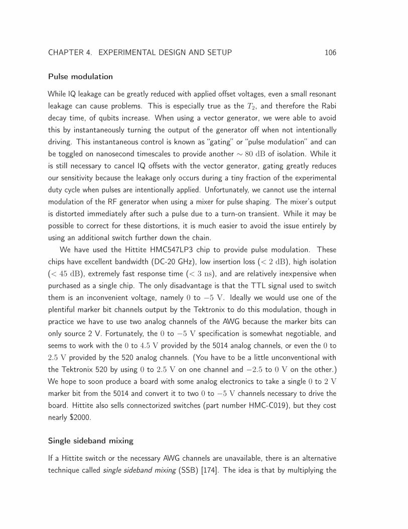
CHAPTER 4. EXPERIMENTAL DESIGN AND SETUP 106
Pulse modulation
While IQ leakage can be greatly reduced with applied offset voltages, even a small resonantleakage can cause problems. This is especially true as the T2, and therefore the Rabidecay time, of qubits increase. When using a vector generator, we were able to avoidthis by instantaneously turning the output of the generator off when not intentionallydriving. This instantaneous control is known as “gating” or “pulse modulation” and canbe toggled on nanosecond timescales to provide another ∼ 80 dB of isolation. While itis still necessary to cancel IQ offsets with the vector generator, gating greatly reducesour sensitivity because the leakage only occurs during a tiny fraction of the experimentalduty cycle when pulses are intentionally applied. Unfortunately, we cannot use the internalmodulation of the RF generator when using a mixer for pulse shaping. The mixer’s outputis distorted immediately after such a pulse due to a turn-on transient. While it may bepossible to correct for these distortions, it is much easier to avoid the issue entirely byusing an additional switch further down the chain.
We have used the Hittite HMC547LP3 chip to provide pulse modulation. Thesechips have excellent bandwidth (DC-20 GHz), low insertion loss (< 2 dB), high isolation(< 45 dB), extremely fast response time (< 3 ns), and are relatively inexpensive whenpurchased as a single chip. The only disadvantage is that the TTL signal used to switchthem is an inconvenient voltage, namely 0 to −5 V. Ideally we would use one of theplentiful marker bit channels output by the Tektronix to do this modulation, though inpractice we have to use two analog channels of the AWG because the marker bits canonly source 2 V. Fortunately, the 0 to −5 V specification is somewhat negotiable, andseems to work with the 0 to 4.5 V provided by the 5014 analog channels, or even the 0 to2.5 V provided by the 520 analog channels. (You have to be a little unconventional withthe Tektronix 520 by using 0 to 2.5 V on one channel and −2.5 to 0 V on the other.)We hope to soon produce a board with some analog electronics to take a single 0 to 2 V
marker bit from the 5014 and convert it to two 0 to −5 V channels necessary to drive theboard. Hittite also sells connectorized switches (part number HMC-C019), but they costnearly $2000.
Single sideband mixing
If a Hittite switch or the necessary AWG channels are unavailable, there is an alternativetechnique called single sideband mixing (SSB) [174]. The idea is that by multiplying the
CHAPTER 4. EXPERIMENTAL DESIGN AND SETUP 107
pulse waveform a sine and cosine of some frequency on the I and Q channels respectively,the resulting pulse frequency will be offset from the local oscillator. Typical SSB frequenciesare 50 to 200 MHz, which means that the LO can be that far detuned from the qubit.The maximum SSB frequency is set by the bandwidth of the Tektronix and the mixer,and was about 300 MHz for the equipment used in this thesis. Additionally, it is possibleto use a single mixer chain to pulse at more than one frequency. This is very useful forpulsing multiple number-split peaks or two separate qubits that are close in frequency.The mathematical details can be found in Blake Johnson’s thesis [152], and have beenimplemented in the Mathematica and Matlab pulse generation code used in the Schoelkopflab. Sideband modulation is also sensitive to two additional non-idealities of the mixer,which, as we will discuss in the next subsection, gives us a convenient method of tuningup their corrections.
IQ skewness and amplitude imbalance
When single sideband mixing is working properly, the only tone going through the mixershould be at the intended frequency (e.g. the LO minus the SSB frequency). However,there are two more tones: one at the LO frequency, and one at the opposite sideband (LOplus the SSB frequency). The tone at the LO frequency is due to IQ leakage, and can becancelled as described in the previous section. The upper sideband, however, is due to twomore sources of mixer imperfection: skewness and amplitude imbalance. The presence ofeither of these errors will cause power to be delivered at this unwanted frequency.
Applied voltages on the I and Q ports should produce RF tones exactly out of phasefrom one another. However, the two ports will not actually be perfectly orthogonal. Wedescribe this imperfection by imagining that the Q axis is rotated by some angle relativeto where it should be, so there is some projection of Q onto I. This skewness syndromecan be corrected by rotating Q back using a linear transformation. (The mathematics ofthis have already been worked out and are included in the pulse generation notebook.)
The same voltages on the I and Q ports should produce the same amount of power atthe RF port. In reality, there is often a small amplitude imbalance between these ports. Ifyou are attenuating the output of the AWG, small differences in the size of the variousattenuators can cause the same error. This will result in a rotation around the x-axis beingdifferent than one around the y-axis for the same nominal voltage. This error is correctedby multiplying one quadrature voltage by some factor.

CHAPTER 4. EXPERIMENTAL DESIGN AND SETUP 108
How do we determine this rotation angle and scale factor? It turns out to be easilydone, as with IQ leakage, using a spectrum analyzer and Tektronix 5014 AWG. First, setthe AWG to play a sequence of a very long (e.g. 15 μs) single-sideband shifted squarewave. Then, using a spectrum analyzer, monitor the power coming out of the mixer atthe unwanted sideband frequency. We then want to adjust the scale factor and angleto minimize this leakage. Changing the scale factor is accomplished by adjusting theamplitude of only one of your two AWG outputs.
Controlling the rotation angle is a bit more subtle. The AWG 5014 has the capabilityof delaying the output of channels relative to one another. This delay is set in multiplesof 5 ps, up to a maximum of several nanoseconds. In the limit of a long SSB-shiftedtone, this delay turns out to be mathematically equivalent to a phase shift according toΔφ = 2πfssbΔt. (Both the Tektronix AWG 520 and the BBN Arbitrary Pulse Sequencerslack this feature, so some other method of determining φ is necessary when using thoseinstruments.) Thus, you can extract the rotation angle and scale factor by iterativelyadjusting the amplitude and channel delay to minimize the upper sideband leakage. Onceknown, these parameters should be incorporated into the sequence file and not left enabledon the AWG. (For short pulses, the AWG delay is not the same as a skewness rotation.)
Filtering
The final mixer correction is also the simplest. The mixers we use (the Marki IQ0618MXP)have a very large RF output at twice the LO frequency. This frequency is so high that it isnot immediately obvious that it would cause problems, but is unsettling in the contextof higher excited states and multi-photon transitions. Fortunately, it is simple to remove:add a band-pass or low-pass filter to the output of either the mixer or power amplifier.For qubits between 6 and 8 GHz, a pair of Mini-Circuits VBFZ-6260-S+ filters work well,but other filters would certainly be acceptable. Where best to place these filters relativeto the amplifier is not obvious. It is beneficial to prevent the large tones from going intothe amplifier to cut down on higher-order products, but it is also advantageous to havethe filters after the amplifier to reduce the noise sent to the fridge. In practice, we havesimply had one filter before and one filter after the amplifier, but it is not clear that itmatters either way.

CHAPTER 4. EXPERIMENTAL DESIGN AND SETUP 109
Tektronix AW
G 5014
20dB
20dB
2Marki IQ0618MXP
Agilent E8257D
I
Q
LORF
Mini-CircuitsZFSC-2-10G
SplitterFrom other mixers
Mini-CircuitsZVE-3W-183+
Mini-CircuitsVBFZ-6260-S+
Splitter
Mini-CircuitsZFSC-2-10G
Meas.tone
Splitter To spectrumanalyzer
To fridge
Mini-CircuitsZFSC-2-10G
Am
p
Figure 4.13: Typical mixer assembly scheme. The components discussed so far areassembled as shown. Multiple qubit channels can be made via the addition of more mixersto the first splitter. To better control reflections, it may be better to split the 20 dB AWGattenuation between either end of the cable – that is, 10 dB at the AWG and 10 dB at themixer. In this scheme, an extra splitter is added right before sending the output to the fridgefor attaching a spectrum analyzer to. It is important to terminate this port when not activelyusing the spectrum analyzer, as the additional cable length going to it can cause problemswith reflections.
4.4.2 Assembly and reflections
A schematic of a typical setup is shown in Fig. 4.13. This scheme is scalable to manyqubits – simply duplicate everything to the right of the first splitter as necessary. If onlyone spectroscopy tone is necessary, omit the first splitter and plug the mixer’s RF portdirectly into the power amplifier. It should be noted that additional savings (compared toa vector generator) can be had by using a cheaper scalar microwave generator known asa LabBrick. It costs a tenth the price or less of a full-featured Agilent scalar generator –$3,000 vs. $35,000 or more. However, compared to Agilent generators, LabBricks havesignificantly worse phase noise, frequency resolution, power precision, and dynamic range.Fortunately, these disadvantages are irrelevant for the single-qubit rotations, though likelyare unacceptable for qubit measurements or biasing of quantum-limited amplifiers.
In addition to knowing which components to use and effective ways of tuning them upindividually, it is important to consider reflections when assembling the apparatus. Anyimpedance mismatch between components can cause reflections of time-dependent pulses,which, when combined with significant lengths of cabling, will result in “ghosts” of yourpulse arriving as much as tens of nanoseconds after the intended pulse. This can causesignificant rotation errors and can be very difficult to diagnose. While it would be best to
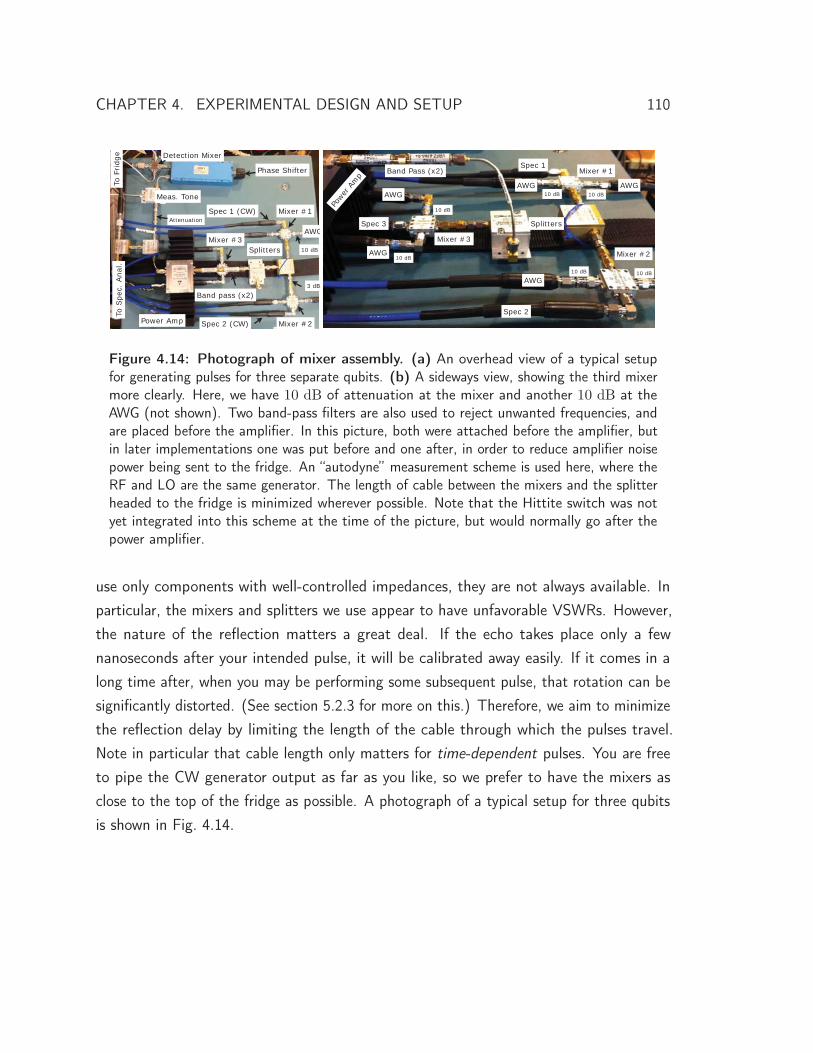
CHAPTER 4. EXPERIMENTAL DESIGN AND SETUP 110
Mixer #1
Mixer #2
Mixer #3
Spec 1 (CW)
Spec 2 (CW)
Splitters
3 dB
Band pass (x2)
10 dB
Power Amp
AWG
To S
pec.
Ana
l.To
Fridg
e
Meas. Tone
Attenuation
Phase Shifter
Detection Mixer
Mixer #2
Mixer #1
Mixer #3
AWG
AWGAWG
Spec 1
Spec 2
Spec 3
AWG
AWG
Splitters
Band Pass (x2)
Power
Am
p
10 dB 10 dB
10 dB10 dB
10 dB
10 dB
Figure 4.14: Photograph of mixer assembly. (a) An overhead view of a typical setupfor generating pulses for three separate qubits. (b) A sideways view, showing the third mixermore clearly. Here, we have 10 dB of attenuation at the mixer and another 10 dB at theAWG (not shown). Two band-pass filters are also used to reject unwanted frequencies, andare placed before the amplifier. In this picture, both were attached before the amplifier, butin later implementations one was put before and one after, in order to reduce amplifier noisepower being sent to the fridge. An “autodyne” measurement scheme is used here, where theRF and LO are the same generator. The length of cable between the mixers and the splitterheaded to the fridge is minimized wherever possible. Note that the Hittite switch was notyet integrated into this scheme at the time of the picture, but would normally go after thepower amplifier.
use only components with well-controlled impedances, they are not always available. Inparticular, the mixers and splitters we use appear to have unfavorable VSWRs. However,the nature of the reflection matters a great deal. If the echo takes place only a fewnanoseconds after your intended pulse, it will be calibrated away easily. If it comes in along time after, when you may be performing some subsequent pulse, that rotation can besignificantly distorted. (See section 5.2.3 for more on this.) Therefore, we aim to minimizethe reflection delay by limiting the length of the cable through which the pulses travel.Note in particular that cable length only matters for time-dependent pulses. You are freeto pipe the CW generator output as far as you like, so we prefer to have the mixers asclose to the top of the fridge as possible. A photograph of a typical setup for three qubitsis shown in Fig. 4.14.
CHAPTER 4. EXPERIMENTAL DESIGN AND SETUP 111
4.5 Conclusions
This chapter introduced the two specific architectures for realizing cQED. The planar or 2Darchitecture, which has been studied extensively in this lab for many years, is the subjectof much of the remaining content of this thesis. We summarized its properties and showedhow the devices are fabricated and packaged. We also introduced a new tunable 3D cQEDarchitecture, which has the useful flux control found in the 2D architecture but also enjoysthe improved qubit lifetimes of 3D qubits. Getting this to work involves re-engineeringevery constituent part, including the “samples” (of which there were two variants, with oneor two cavities), the sample holders, the qubits, and the flux bias lines. We also showedthree generations of flux bias line designs, each implementing more sophisticated filteringthan its predecessor. Finally, we discussed how these samples are cooled in dilution fridgesand operated with an overview of the room-temperature control equipment involved. It ispossible to use either a vector-modulated RF generator to generate our microwave controlpulses, or, with proper calibrations, a much cheaper scalar generator and RF mixer. Inthe next chapter, we will go into detail about the initial measurements to bring a newqubit experiment online, the best way to accurately tune-up single-qubit rotations, and willintroduce the basic single-qubit experiments that we will use as tools in future chapters.

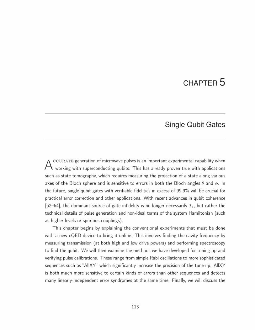
CHAPTER 5
Single Qubit Gates
Accurate generation of microwave pulses is an important experimental capability whenworking with superconducting qubits. This has already proven true with applications
such as state tomography, which requires measuring the projection of a state along variousaxes of the Bloch sphere and is sensitive to errors in both the Bloch angles θ and φ. Inthe future, single qubit gates with verifiable fidelities in excess of 99.9% will be crucial forpractical error correction and other applications. With recent advances in qubit coherence[62–64], the dominant source of gate infidelity is no longer necessarily T1, but rather thetechnical details of pulse generation and non-ideal terms of the system Hamiltonian (suchas higher levels or spurious couplings).
This chapter begins by explaining the conventional experiments that must be donewith a new cQED device to bring it online. This involves finding the cavity frequency bymeasuring transmission (at both high and low drive powers) and performing spectroscopyto find the qubit. We will then examine the methods we have developed for tuning up andverifying pulse calibrations. These range from simple Rabi oscillations to more sophisticatedsequences such as “AllXY” which significantly increase the precision of the tune-up. AllXYis both much more sensitive to certain kinds of errors than other sequences and detectsmany linearly-independent error syndromes at the same time. Finally, we will discuss the
113
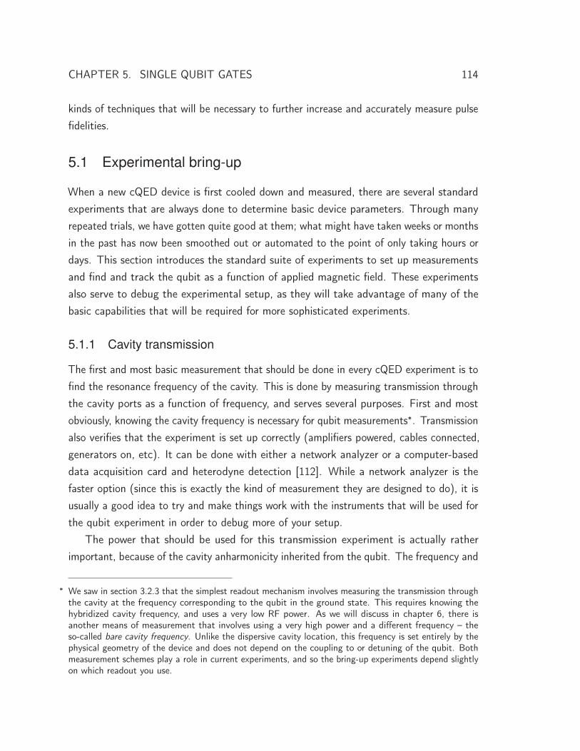
CHAPTER 5. SINGLE QUBIT GATES 114
kinds of techniques that will be necessary to further increase and accurately measure pulsefidelities.
5.1 Experimental bring-up
When a new cQED device is first cooled down and measured, there are several standardexperiments that are always done to determine basic device parameters. Through manyrepeated trials, we have gotten quite good at them; what might have taken weeks or monthsin the past has now been smoothed out or automated to the point of only taking hours ordays. This section introduces the standard suite of experiments to set up measurementsand find and track the qubit as a function of applied magnetic field. These experimentsalso serve to debug the experimental setup, as they will take advantage of many of thebasic capabilities that will be required for more sophisticated experiments.
5.1.1 Cavity transmission
The first and most basic measurement that should be done in every cQED experiment is tofind the resonance frequency of the cavity. This is done by measuring transmission throughthe cavity ports as a function of frequency, and serves several purposes. First and mostobviously, knowing the cavity frequency is necessary for qubit measurements∗. Transmissionalso verifies that the experiment is set up correctly (amplifiers powered, cables connected,generators on, etc). It can be done with either a network analyzer or a computer-baseddata acquisition card and heterodyne detection [112]. While a network analyzer is thefaster option (since this is exactly the kind of measurement they are designed to do), it isusually a good idea to try and make things work with the instruments that will be used forthe qubit experiment in order to debug more of your setup.
The power that should be used for this transmission experiment is actually ratherimportant, because of the cavity anharmonicity inherited from the qubit. The frequency and
∗ We saw in section 3.2.3 that the simplest readout mechanism involves measuring the transmission throughthe cavity at the frequency corresponding to the qubit in the ground state. This requires knowing thehybridized cavity frequency, and uses a very low RF power. As we will discuss in chapter 6, there isanother means of measurement that involves using a very high power and a different frequency – theso-called bare cavity frequency. Unlike the dispersive cavity location, this frequency is set entirely by thephysical geometry of the device and does not depend on the coupling to or detuning of the qubit. Bothmeasurement schemes play a role in current experiments, and so the bring-up experiments depend slightlyon which readout you use.
CHAPTER 5. SINGLE QUBIT GATES 115
0.06
0.04
0.02
0.009.169.139.109.07
Frequency (GHz)
-34 dBm0.6
0.4
0.2
0.09.169.139.109.07
Frequency (GHz)
+6 dBm
30
20
10
0Msm
't vo
ltage
(mV
)
9.169.139.109.07Frequency (GHz)
+20 dBm
(a) (b) (c)
Figure 5.1: Cavity transmission for various drive strengths. (a) Transmission using arelatively large drive strength (+20 dBm), showing the “bare cavity” frequency and linearresponse of the resonator. (b) As we turn down power (to +6 dBm), the cavity revealsa strongly nonlinear response, indicating the presence of a qubit which is hybridizing withthe cavity mode. (c) At sufficiently low drive strengths (-34 dBm), the cavity has a meanoccupation of only one photon and returns to linear response at its “low power” frequencyused for dispersive readout. Notice the differing y-scales for each case.
structure of cavity transmission depends very strongly on input power, which is the basisof the high-power readout scheme [59] described in section 6.3. As shown in Fig. 5.1(a-c),we see that, as we lower the drive power, the lineshape of transmission changes froma lorentzian response at the bare cavity frequency at high power, to a highly nonlinearresponse at medium power, and finally to a weak lorentzian response at the dispersivelyshifted frequency at very low (∼ 1 photon mean excitation) power. This behavior is onlypresent when a qubit is strongly coupled to the cavity, so seeing any non-linear powerdependence of the cavity frequency and response is an easy way to detect the presenceof qubits. It makes sense to first use a relatively large amount of power to find the barecavity frequency and then repeat the measurement with substantially less power to tryand detect the presence of nonlinearity.
In experiments where a low-power dispersive readout mechanism is going to be used,measuring the frequency of the cavity at ∼ 1 photon mean occupation is necessary. Sinceknowing the input power required to drive one photon is a function of line attenuation,cavity Q, and other parameters that may only be roughly known, a good tactic is to turndown the drive power until the apparent cavity frequency stops changing. Especially in thecase of high Q cavities, this may become impractical if the signal becomes too small. Inthat case, once the qubit is found, number splitting (section 3.2.3) can be used to moreefficiently measure the ultra-low power cavity frequency. In experiments where the qubit
CHAPTER 5. SINGLE QUBIT GATES 116
9.6
9.4
9.2
9.0
8.8
Freq
uenc
y (G
Hz)
-1.2 -0.8 -0.4 0.0Vbias [V]
Figure 5.2: Transmission vs. applied qubit flux. When the qubit frequency is tunedthrough the cavity, the two hybridize and make an avoided crossing. This is known asa vacuum-Rabi splitting. These data were taken using the four-qubit device described insection 7.1.
frequency can be changed, the low-power cavity frequency will also move, and must befound at every magnetic flux. This is in contrast to the high-power bare cavity frequency,which is independent of qubit detuning. It is also worth noting that the difference betweenthe high-power and low-power cavity frequencies and the approximate coupling strength ofthe qubit and cavity can be used to calculate the qubit detuning. If these frequencies arealmost the same, the qubit is weakly coupled and/or far detuned.
Measuring transmission as a function of qubit frequency can also inform you aboutdevice parameters. If the qubit’s maximum frequency (at the zero SQUID flux point) isabove the cavity, tuning the qubit through the cavity will produce vacuum-Rabi splittingcurve like the one shown in Fig. 5.2. There, as described in section 3.2.2, the cavityresponse splits into two peaks because of the avoided crossing between the cavity andqubit. The size of this splitting indicates the coupling strength between the two. Evenif the qubit does not actually come into resonance, the cavity will still shift in frequencyaway from the qubit as it approaches. This can be useful for finding the magnetic fieldcorresponding to the maximum qubit frequency since it is usually offset from 0 by ambientmagnetic fields. In either case of maximum qubit frequency, the conversion of appliedcontrol voltage to SQUID flux quanta can be measured by tuning over a full period of flux.

CHAPTER 5. SINGLE QUBIT GATES 117
5.1.2 Spectroscopy
The next experiment generally performed to bring-up an experiment is spectroscopy. Thereare several variations commonly used in the field, but they all involve applying a microwavepulse at some frequency followed by a qubit measurement∗. The frequency of the pulse istypically scanned and, when it drives transitions of the qubit, the subsequent measurementwill indicate as such. The simplest conceptual version of spectroscopy is known as pulsedspectroscopy, where the qubit pulse is turned off prior to a measurement being turned on.The qubit pulse could either be some fast gaussian rotation, or more commonly, a longsaturation tone. A tone that is much longer than the qubit T2 will drive some equilibriumincoherent population of the qubit, and is convenient because that population is relativelyinsensitive to the pulse power. (A short, coherent drive would require carefully tuning theπ pulse power at each detuning to maximize fidelity, and could even eliminate signal if weinadvertently drive a 2nπ pulse. However, this approach can yield a larger signal if SNR isa challenge.) The spectral width of a long pulse is much smaller than the faster gaussian,which allows for narrower line widths. An example of saturation pulsed spectroscopy isshown in Fig. 5.3(a).
Prior to the high-power readout coming into common usage [59], spectroscopy wasmore often done with both the qubit saturation and measurement tones on continuously.One would step the frequency of a continuous-wave (CW) microwave tone while monitoringthe transmission of second tone at the low-power dressed cavity frequency to detect qubittransitions [114]. This is known as “CW spectroscopy.” Since this approach does notrequire time-domain control it is quite straightforward to set up. It has the disadvantageof producing a more-complicated spectrum than pulsed spectroscopy, however. There isan equilibrium population of photons in the cavity, so qubit transitions that depend on thenumber of photons will be visible. The most concrete example of this is qubit number-splitting (section 3.2.3) which will either split or broaden the qubit response, thoughhigher-order transitions may also be visible. This is in contrast to pulsed spectroscopy,where only one microwave pulse at a time is ever on and many of these complications areabsent. CW spectroscopy is also incompatible with the high-power readout mechanism,
∗ In addition to pulsed and CW spectroscopy discussed here, we will later introduce “swap spectroscopy”as well as “flux spectroscopy” which add a fast-flux pulse to the mix. They serve to measure avoidedcrossings in the time domain, which is vital to calibrating sudden entangling gates or to calibrate fluxpulse amplitudes. The second of these is a requirement when using fast flux to quantitatively measure asystem.

CHAPTER 5. SINGLE QUBIT GATES 118
since the qubit state is scrambled by the measurement tone, so finding the dressed cavityfrequency for each detuning is necessary. The experimental simplicity of CW spectroscopyis often out-weighed by the convenience and high fidelity of the high-power readout, soCW spectroscopy is seldom performed anymore.
When using a long saturation tone for spectroscopy, the drive strength is an importantconsideration. As described in Ref. 175, at low drive power, the spectroscopic linewidth ofthe qubit is set by the pure dephasing time T ∗
2 . This is because the inverse of this numbercan be taken as the intrinsic uncertainty of the qubit frequency. As the power of the drive isincreased, the observed linewidth will also grow, a phenomenon known as power broadening.The expected power dependence is given by 2πΔfHWHM =
√1/T 2
2 + 4Ω2RT1/T2, where
T1 and T2 are the qubit lifetime and dephasing time and ΩR is the drive Rabi rate [175].It can be understood as the drive causing stimulated emission of the qubit, shortening itslifetime and therefore T ∗
2 . Power broadening is actually a useful effect, since recent 3Dqubits can have intrinsic linewidths less than 10 KHz [62] and would be difficult to findwithout substantial broadening. Moreover, as the applied power is increased, the averageexcited state qubit population initially grows linearly, and so its response gets stronger. Forlarger drive strengths, the average qubit population approaches 1/2 and saturates. Thepower dependence of the qubit transition is shown in Fig. 5.3(b-c).
A large spectroscopy power can also drive higher-order qubit transitions. For example, atwo-photon transition directly from the ground state to the second excited state (|0〉 → |2〉)is allowed, but requires substantially more drive power than it takes to saturate |0〉 → |1〉.This is shown in the blue trace of Fig. 5.3(a). This effect is very useful in that it isthe easiest way to directly measure qubit anharmonicity. The transition frequencies arerelated by ω02/2 = (ω01 + ω12) /2, and ω12 = ω01 + α, where α is defined as the qubitanharmonicity. Finding both the ω01 and ω02/2 transitions, therefore, also determinesα. The fact that this is the anharmonicity can be verified by saturating the 0 → 1
transition with a CW tone and then repeating spectroscopy, directly revealing the 1 → 2
transition. Even higher-order qubit transitions, such as a three-photon transition directlyfrom |0〉 → |3〉 are also allowed. When two qubits are coupled to the same cavity, atwo-photon transition between |00〉 → |11〉 is also possible at the exact average of thetwo qubit transition frequencies, and is sometimes referred to a “Bell-Rabi” transitionbecause it can be used to directly prepare an entangled Bell state [176]. Thus, if you seea spurious transition in your spectrum it is often a good idea to first try turning down

CHAPTER 5. SINGLE QUBIT GATES 119
Figure 5.3: Qubit spectroscopy. (a) In black, spectroscopy of a 3D qubit is performedwith a low drive power. Blue shows the same trace with significantly more power, broadeningthe 0 → 1 qubit transition and turning on a two-photon transition directly between |0〉 and|2〉. Knowing both of these frequencies tells you the qubit anharmonicity. This is verified witha third experiment, shown in red, where the 0 → 1 transition is saturated with a CW toneand spectroscopy is done with a second tone, revealing the 1 → 2 transition. The differencebetween these two frequencies is a direct measure of anharmonicity, with the f02/2 transitionlocated directly between. (b) The f01 transition as a function of drive power, demonstratingpower broadening. (c) The FWHM of the qubit transition as a function of spectroscopy drivepower, fit to the expected power dependence. (Figure adapted with permission from [62].See Copyright Permissions.).
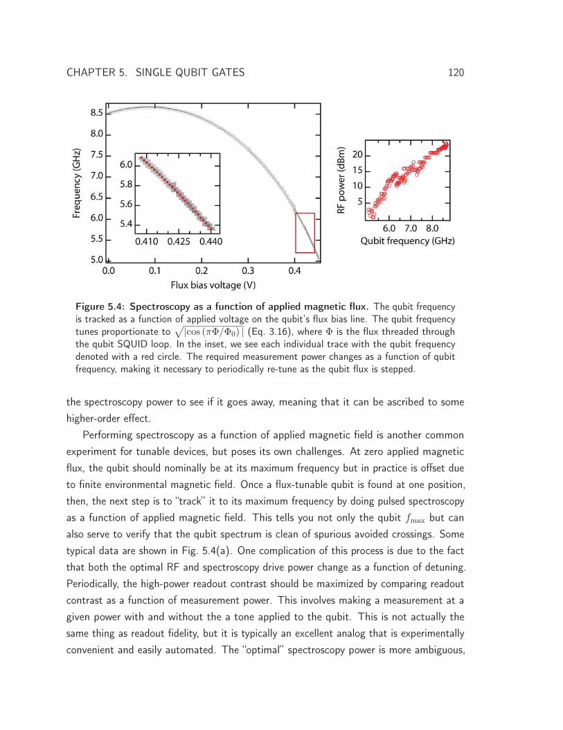
CHAPTER 5. SINGLE QUBIT GATES 120
Figure 5.4: Spectroscopy as a function of applied magnetic flux. The qubit frequencyis tracked as a function of applied voltage on the qubit’s flux bias line. The qubit frequencytunes proportionate to
√|cos (πΦ/Φ0) | (Eq. 3.16), where Φ is the flux threaded throughthe qubit SQUID loop. In the inset, we see each individual trace with the qubit frequencydenoted with a red circle. The required measurement power changes as a function of qubitfrequency, making it necessary to periodically re-tune as the qubit flux is stepped.
the spectroscopy power to see if it goes away, meaning that it can be ascribed to somehigher-order effect.
Performing spectroscopy as a function of applied magnetic field is another commonexperiment for tunable devices, but poses its own challenges. At zero applied magneticflux, the qubit should nominally be at its maximum frequency but in practice is offset dueto finite environmental magnetic field. Once a flux-tunable qubit is found at one position,then, the next step is to “track” it to its maximum frequency by doing pulsed spectroscopyas a function of applied magnetic field. This tells you not only the qubit fmax but canalso serve to verify that the qubit spectrum is clean of spurious avoided crossings. Sometypical data are shown in Fig. 5.4(a). One complication of this process is due to the factthat both the optimal RF and spectroscopy drive power change as a function of detuning.Periodically, the high-power readout contrast should be maximized by comparing readoutcontrast as a function of measurement power. This involves making a measurement at agiven power with and without the a tone applied to the qubit. This is not actually thesame thing as readout fidelity, but it is typically an excellent analog that is experimentallyconvenient and easily automated. The “optimal” spectroscopy power is more ambiguous,
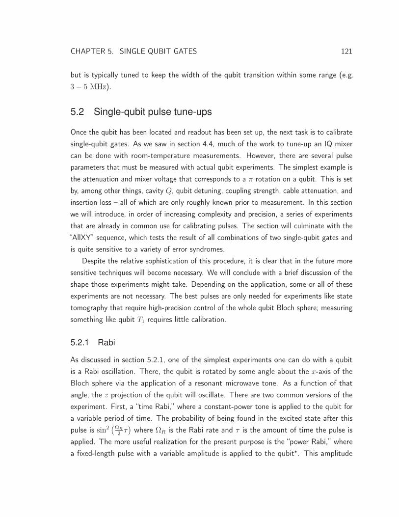
CHAPTER 5. SINGLE QUBIT GATES 121
but is typically tuned to keep the width of the qubit transition within some range (e.g.3 − 5 MHz).
5.2 Single-qubit pulse tune-ups
Once the qubit has been located and readout has been set up, the next task is to calibratesingle-qubit gates. As we saw in section 4.4, much of the work to tune-up an IQ mixercan be done with room-temperature measurements. However, there are several pulseparameters that must be measured with actual qubit experiments. The simplest example isthe attenuation and mixer voltage that corresponds to a π rotation on a qubit. This is setby, among other things, cavity Q, qubit detuning, coupling strength, cable attenuation, andinsertion loss – all of which are only roughly known prior to measurement. In this sectionwe will introduce, in order of increasing complexity and precision, a series of experimentsthat are already in common use for calibrating pulses. The section will culminate with the“AllXY” sequence, which tests the result of all combinations of two single-qubit gates andis quite sensitive to a variety of error syndromes.
Despite the relative sophistication of this procedure, it is clear that in the future moresensitive techniques will become necessary. We will conclude with a brief discussion of theshape those experiments might take. Depending on the application, some or all of theseexperiments are not necessary. The best pulses are only needed for experiments like statetomography that require high-precision control of the whole qubit Bloch sphere; measuringsomething like qubit T1 requires little calibration.
5.2.1 Rabi
As discussed in section 5.2.1, one of the simplest experiments one can do with a qubitis a Rabi oscillation. There, the qubit is rotated by some angle about the x-axis of theBloch sphere via the application of a resonant microwave tone. As a function of thatangle, the z projection of the qubit will oscillate. There are two common versions of theexperiment. First, a “time Rabi,” where a constant-power tone is applied to the qubit fora variable period of time. The probability of being found in the excited state after thispulse is sin2
(ΩR
2τ)
where ΩR is the Rabi rate and τ is the amount of time the pulse isapplied. The more useful realization for the present purpose is the “power Rabi,” wherea fixed-length pulse with a variable amplitude is applied to the qubit∗. This amplitude
CHAPTER 5. SINGLE QUBIT GATES 122
8.5
8.4
8.3
8.2
8.1
8.0Spec
. fre
quen
cy (G
Hz)
1.351.301.25Virtual yoko voltage (V)
4
3
2
806040200Rabi sequence number
8.29 GHz(a) (b) (c)
47
46
45
Msm
't vo
ltage
(mV
)
806040200Rabi sequence number
Figure 5.5: Rabi oscillations. (a) A qubit is rotated by some angle θ, controlled by theamplitude of a resonant gaussian microwave pulse, and measured. The x-axis of this plot isexperiment number, where 41 has no rotation, experiments greater than 41 have positiverotation angles, and lesser have negative ones. For example, point 19 corresponds to a −πrotation. (b) A “bad” Rabi oscillation showing that the qubit is hybridized with some otherHilbert space. A 2π (e.g. sequence number 0 or 80) pulse does not return the qubit to theground state, indicating leakage from the qubit computational space. (c) Spectroscopy in thevicinity of an avoided crossing. The red arrow indicates the frequency and bias of the qubitin (b), showing that the system is indeed hybridized with some spurious degree of freedom.
is swept, again yielding a sinusoidal response. To tune-up the sequence, we adjust theRabi rate so that a π rotation happens at some desired voltage or DAC value. All possiblerotation angles can be interpolated from that calibration as long as the pulse amplitudemodulation is linear in voltage. An example of this is shown in Fig. 5.5(a).
A Rabi experiment also serves as a general check of whether a qubit is behaving well.The oscillation is only perfect in the limit of addressing a true two-level system, and so ifthis assumption is violated, the resulting curve will be distorted. This may come about,for example, if the bandwidth of the qubit pulse is comparable to the anharmonicity of thequbit or if the qubit is hybridized with some other degree of freedom (such as a two-levelsystem or a cavity mode). An example of this second case is shown in Fig. 5.5(b). Thisqubit was near a spurious avoided crossing, shown in (c), distorting the oscillation. A 2π
pulse does not return the qubit to its ground state, indicating that there is leakage fromthe two-level qubit Hilbert space. Another common distortion is an overall offset of thecurve along the x-axis because of mixer IQ leakage (which drives an equilibrium qubit
∗ A time Rabi is exactly equivalent to a power Rabi from the point of view of the physics, but it isexperimentally convenient to impose a constant time for pulses and vary amplitudes. This is true notonly because it is easier to time things out when you have “clock cycles,” but also because the amplituderesolution of AWGs is typically much better than their time resolution.
CHAPTER 5. SINGLE QUBIT GATES 123
excited state population). It is also not unusual to see that a negative and positive pulseamplitude drive different apparent rotations, which might be due to a mixer nonlinearity orimbalance. Generally, a Rabi oscillation will not look as good as shown in Fig. 5.5(a) unlessboth the mixer (see section 4.4.1) and pulse parameters (enumerated in section 5.2.3)have been tuned carefully.
5.2.2 Ramsey
As we described in section 5.1.2, the rough frequency of the qubit is first determined withpulsed spectroscopy. However, because of power broadening and finite pulse bandwidth,this procedure typically enjoys a precision of only ∼ 1 MHz. That experiment typicallywill not use a mixer, and so the frequency measured there might also have a systematicoffset from the one you will have in the “real” time-domain experiment. This might be dueto Stark shifts from IQ leakage or equilibrium cavity photon population due to a too-fastexperimental repetition rate. Thus, the precise qubit frequency must be measured using aRamsey experiment.
A Ramsey oscillation is the gold-standard of frequency calibration for qubits as wellas for precision instruments like atomic clocks [177]. The idea is to use the fact that adetuning Δ of the qubit from the RF generator frequency reference looks like a z-gatebeing continuously applied at a rate Δ. Thus, even tiny detunings can be measured byintegrating this detuning as a function of time, limited only by the pure dephasing rate T ∗
2 .The procedure begins by putting the qubit on the equator of the Bloch sphere with a π/2
pulse. (Though errors in this rotation angle merely reduces the contrast of the Ramseyfringes.) The qubit is then allowed to evolve for some period of time before a second π/2
rotation is applied. For a finite detuning, the qubit will oscillate between being rotatedback to the ground state and the excited state as a function of the delay time. Because ofdephasing, the amplitude of this oscillation will exponentially decay∗ at a rate T ∗
2 .In order to distinguish between the exponential decay due to dephasing and the
oscillation due to detuning, it is desirable to have four or five full oscillations in the firsttwo 1/e times. Thus, you should either intentionally detune from where you think the
∗ This is also the standard method of measuring the qubit decoherence time T ∗2 . Another common version
of this procedure includes a π pulse on the qubit exactly between the two π/2 pulses – this is knownas a Hahn echo. The π pulse flips the direction of evolution, thereby making the qubit insensitive tolow-frequency noise [178]. This will increase the effective coherence time, known as T echo
2 , when thespectrum of the qubit noise is skewed toward lower frequencies, as it often is.
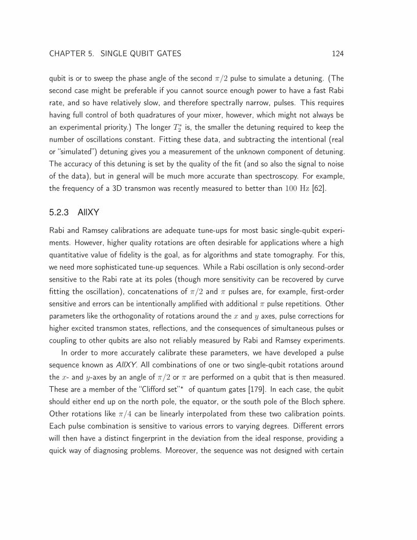
CHAPTER 5. SINGLE QUBIT GATES 124
qubit is or to sweep the phase angle of the second π/2 pulse to simulate a detuning. (Thesecond case might be preferable if you cannot source enough power to have a fast Rabirate, and so have relatively slow, and therefore spectrally narrow, pulses. This requireshaving full control of both quadratures of your mixer, however, which might not always bean experimental priority.) The longer T ∗
2 is, the smaller the detuning required to keep thenumber of oscillations constant. Fitting these data, and subtracting the intentional (realor “simulated”) detuning gives you a measurement of the unknown component of detuning.The accuracy of this detuning is set by the quality of the fit (and so also the signal to noiseof the data), but in general will be much more accurate than spectroscopy. For example,the frequency of a 3D transmon was recently measured to better than 100 Hz [62].
5.2.3 AllXY
Rabi and Ramsey calibrations are adequate tune-ups for most basic single-qubit experi-ments. However, higher quality rotations are often desirable for applications where a highquantitative value of fidelity is the goal, as for algorithms and state tomography. For this,we need more sophisticated tune-up sequences. While a Rabi oscillation is only second-ordersensitive to the Rabi rate at its poles (though more sensitivity can be recovered by curvefitting the oscillation), concatenations of π/2 and π pulses are, for example, first-ordersensitive and errors can be intentionally amplified with additional π pulse repetitions. Otherparameters like the orthogonality of rotations around the x and y axes, pulse corrections forhigher excited transmon states, reflections, and the consequences of simultaneous pulses orcoupling to other qubits are also not reliably measured by Rabi and Ramsey experiments.
In order to more accurately calibrate these parameters, we have developed a pulsesequence known as AllXY. All combinations of one or two single-qubit rotations aroundthe x- and y-axes by an angle of π/2 or π are performed on a qubit that is then measured.These are a member of the “Clifford set”∗ of quantum gates [179]. In each case, the qubitshould either end up on the north pole, the equator, or the south pole of the Bloch sphere.Other rotations like π/4 can be linearly interpolated from these two calibration points.Each pulse combination is sensitive to various errors to varying degrees. Different errorswill then have a distinct fingerprint in the deviation from the ideal response, providing aquick way of diagnosing problems. Moreover, the sequence was not designed with certain
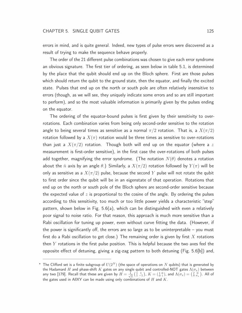
CHAPTER 5. SINGLE QUBIT GATES 125
errors in mind, and is quite general. Indeed, new types of pulse errors were discovered as aresult of trying to make the sequence behave properly.
The order of the 21 different pulse combinations was chosen to give each error syndromean obvious signature. The first tier of ordering, as seen below in table 5.1, is determinedby the place that the qubit should end up on the Bloch sphere. First are those pulseswhich should return the qubit to the ground state, then the equator, and finally the excitedstate. Pulses that end up on the north or south pole are often relatively insensitive toerrors (though, as we will see, they uniquely indicate some errors and so are still importantto perform), and so the most valuable information is primarily given by the pulses endingon the equator.
The ordering of the equator-bound pulses is first given by their sensitivity to over-rotations. Each combination varies from being only second-order sensitive to the rotationangle to being several times as sensitive as a normal π/2 rotation. That is, a X(π/2)
rotation followed by a X(π) rotation would be three times as sensitive to over-rotationsthan just a X(π/2) rotation. Though both will end up on the equator (where a z
measurement is first-order sensitive), in the first case the over-rotations of both pulsesadd together, magnifying the error syndrome. (The notation N(θ) denotes a rotationabout the n axis by an angle θ.) Similarly, a X(π/2) rotation followed by Y (π) will beonly as sensitive as a X(π/2) pulse, because the second Y pulse will not rotate the qubitto first order since the qubit will be in an eigenstate of that operation. Rotations thatend up on the north or south pole of the Bloch sphere are second-order sensitive becausethe expected value of z is proportional to the cosine of the angle. By ordering the pulsesaccording to this sensitivity, too much or too little power yields a characteristic “step”pattern, shown below in Fig. 5.6(a), which can be distinguished with even a relativelypoor signal to noise ratio. For that reason, this approach is much more sensitive than aRabi oscillation for tuning up power, even without curve fitting the data. (However, ifthe power is significantly off, the errors are so large as to be uninterpretable – you mustfirst do a Rabi oscillation to get close.) The remaining order is given by first X rotationsthen Y rotations in the first pulse position. This is helpful because the two axes feel theopposite effect of detuning, giving a zig-zag pattern to both detuning (Fig. 5.6[b]) and,
∗ The Clifford set is a finite subgroup of U(2N ) (the space of operations on N qubits) that is generated bythe Hadamard H and phase-shift K gates on any single qubit and controlled-NOT gates Λ(σx) betweenany two [179]. Recall that these are given by H = 1√
2
(1 11 −1
), K = ( 1 0
0 i ), and Λ(σx) =(I 00 σx
). All of
the gates used in AllXY can be made using only combinations of H and K.

CHAPTER 5. SINGLE QUBIT GATES 126
Ideal 〈z〉 First pulse Second pulse Power dependence Detuning dependence1 Id Id 1 11 X(π) X(π) 1 − 8ε2 + O(ε4) 1 − π2ε4
32 + O(ε6)
1 Y (π) Y (π) 1 − 8ε2 + O(ε4) 1 − π2ε4
32 + O(ε6)
1 X(π) Y (π) 1 − 4ε2 + O(ε4) 1 − ε2 + O(ε3)
1 Y (π) X(π) 1 − 4ε2 + O(ε4) 1 − ε2 − O(ε3)
0 X(π/2) Id −ε+ O(ε3) (1 − π2 )ε
2 − O(ε4)
0 Y (π/2) Id −ε+ O(ε3) (1 − π2 )ε
2 − O(ε4)
0 X(π/2) Y (π/2) ε2 − O(ε4) −2ε+ O(ε3)
0 Y (π/2) X(π/2) ε2 − O(ε4) 2ε − O(ε3)
0 X(π/2) Y (π) ε − O(ε3) −ε − O(ε2)
0 Y (π/2) X(π) ε − O(ε3) ε − O(ε2)
0 X(π) Y (π/2) ε − O(ε3) −ε − O(ε2)
0 Y (π) X(π/2) ε − O(ε3) ε − O(ε2)
0 X(π/2) X(π) 3ε − O(ε3) 3πε2
8 + O(ε4)
0 X(π) X(π/2) 3ε − O(ε3) 3πε2
8 + O(ε4)
0 Y (π/2) Y (π) 3ε − O(ε3) 3πε2
8 + O(ε4)
0 Y (π) Y (π/2) 3ε − O(ε3) 3πε2
8 + O(ε4)
-1 X(π) Id −1 + 2ε2 + O(ε4) −1 + ε2
2 + O(ε4)
-1 Y (π) Id −1 + 2ε2 + O(ε4) −1 + ε2
2 + O(ε4)
-1 X(π/2) X(π/2) −1 + 2ε2 + O(ε4) −1 + 2ε2 + O(ε4)
-1 Y (π/2) Y (π/2) −1 + 2ε2 + O(ε4) −1 + 2ε2 + O(ε4)
Table 5.1: AllXY pulse sequence. The first and second pulse are listed and orderedaccording to where the qubit should ideally end up (on the north, equator, or south poleof the Bloch sphere). The analytically calculated leading-order power and detuning errordependence of the qubit z projection are shown.
as we will see later, an additional pulse parameter used to compensate for phase errorsdue to the presence of higher excited-state levels being incorrect [180]. The leading-orderdependence on small errors of amplitude and detuning are listed in the table (the codeused to produce these equations is found in appendix B).
Single-qubit error syndromes
As mentioned in the previous section, the AllXY sequence is set up so that the myriadpulse error types produce distinct error syndromes. While many of these syndromes canbe calculated with unitary matrix multiplication, others are due to either physical flaws in
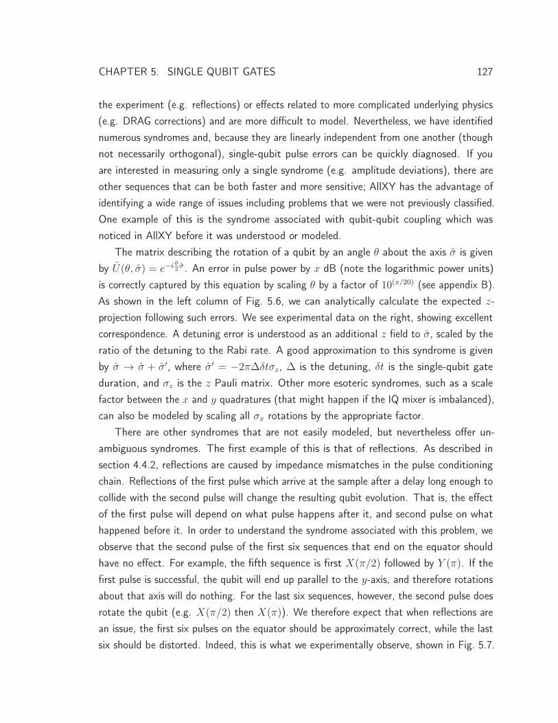
CHAPTER 5. SINGLE QUBIT GATES 127
the experiment (e.g. reflections) or effects related to more complicated underlying physics(e.g. DRAG corrections) and are more difficult to model. Nevertheless, we have identifiednumerous syndromes and, because they are linearly independent from one another (thoughnot necessarily orthogonal), single-qubit pulse errors can be quickly diagnosed. If youare interested in measuring only a single syndrome (e.g. amplitude deviations), there areother sequences that can be both faster and more sensitive; AllXY has the advantage ofidentifying a wide range of issues including problems that we were not previously classified.One example of this is the syndrome associated with qubit-qubit coupling which wasnoticed in AllXY before it was understood or modeled.
The matrix describing the rotation of a qubit by an angle θ about the axis σ is givenby U(θ, σ) = e−i θ
2σ. An error in pulse power by x dB (note the logarithmic power units)
is correctly captured by this equation by scaling θ by a factor of 10(x/20) (see appendix B).As shown in the left column of Fig. 5.6, we can analytically calculate the expected z-projection following such errors. We see experimental data on the right, showing excellentcorrespondence. A detuning error is understood as an additional z field to σ, scaled by theratio of the detuning to the Rabi rate. A good approximation to this syndrome is givenby σ → σ + σ′, where σ′ = −2πΔδtσz, Δ is the detuning, δt is the single-qubit gateduration, and σz is the z Pauli matrix. Other more esoteric syndromes, such as a scalefactor between the x and y quadratures (that might happen if the IQ mixer is imbalanced),can also be modeled by scaling all σx rotations by the appropriate factor.
There are other syndromes that are not easily modeled, but nevertheless offer un-ambiguous syndromes. The first example of this is that of reflections. As described insection 4.4.2, reflections are caused by impedance mismatches in the pulse conditioningchain. Reflections of the first pulse which arrive at the sample after a delay long enough tocollide with the second pulse will change the resulting qubit evolution. That is, the effectof the first pulse will depend on what pulse happens after it, and second pulse on whathappened before it. In order to understand the syndrome associated with this problem, weobserve that the second pulse of the first six sequences that end on the equator shouldhave no effect. For example, the fifth sequence is first X(π/2) followed by Y (π). If thefirst pulse is successful, the qubit will end up parallel to the y-axis, and therefore rotationsabout that axis will do nothing. For the last six sequences, however, the second pulse doesrotate the qubit (e.g. X(π/2) then X(π)). We therefore expect that when reflections arean issue, the first six pulses on the equator should be approximately correct, while the lastsix should be distorted. Indeed, this is what we experimentally observe, shown in Fig. 5.7.

CHAPTER 5. SINGLE QUBIT GATES 128
-1.0
-0.5
0.0
0.5
1.0
Z pr
ojec
tion
IdId
XpXp
YpYp
XpYp
YpXp
X9Id
Y9Id
X9Y9
Y9X9
X9Yp
Y9Xp
XpY9
YpX9
X9Xp
XpX9
Y9Yp
YpY9
XpId
YpId
X9X9
Y9Y9
IdId
XpXp
YpYp
XpYp
YpXp
X9Id
Y9Id
X9Y9
Y9X9
X9Yp
Y9Xp
XpY9
YpX9
X9Xp
XpX9
Y9Yp
YpY9
XpId
YpId
X9X9
Y9Y9
Power Scale +1.0 dB +0.8 dB +0.6 dB +0.4 dB +0.2 dB 0.0 dB -0.2 dB -0.4 dB -0.6 dB -0.8 dB -1.0 dB
-1.0
-0.5
0.0
0.5
1.0
Z pr
ojec
tion
IdId
XpXp
YpYp
XpYp
YpXp
X9Id
Y9Id
X9Y9
Y9X9
X9Yp
Y9Xp
XpY9
YpX9
X9Xp
XpX9
Y9Yp
YpY9
XpId
YpId
X9X9
Y9Y9
IdId
XpXp
YpYp
XpYp
YpXp
X9Id
Y9Id
X9Y9
Y9X9
X9Yp
Y9Xp
XpY9
YpX9
X9Xp
XpX9
Y9Yp
YpY9
XpId
YpId
X9X9
Y9Y9
Detuning -10MHz -8 MHz -6 MHz -4 MHz -2 MHz 0 MHz +2 MHz +4 MHz +6 MHz +8 MHz +10MHz
IdId
XpXp
YpYp
XpYp
YpXp
X9Id
Y9Id
X9Y9
Y9X9
X9Yp
Y9Xp
XpY9
YpX9
X9Xp
XpX9
Y9Yp
YpY9
XpId
YpId
X9X9
Y9Y9
Pulse sequence
X Scaling 1.05 1.04 1.03 1.02 1.01 1.00 0.99 0.98 0.97 0.96 0.95
-1.0
-0.5
0.0
0.5
1.0
Z pr
ojec
tion
IdId
XpXp
YpYp
XpYp
YpXp
X9Id
Y9Id
X9Y9
Y9X9
X9Yp
Y9Xp
XpY9
YpX9
X9Xp
XpX9
Y9Yp
YpY9
XpId
YpId
X9X9
Y9Y9
Pulse sequence
Calculation Experiment(a)
(b)
(c)
Figure 5.6: Experimental and simulated syndromes for amplitude, detuning, andskew-type errors. On the left, a calculation using unitary matrix evolution for each typeof error are shown. The right shows the experimental reproduction of these same errors,showing excellent correspondence. Each error signature is distinct, making it possible todetect several error syndromes simultaneously.
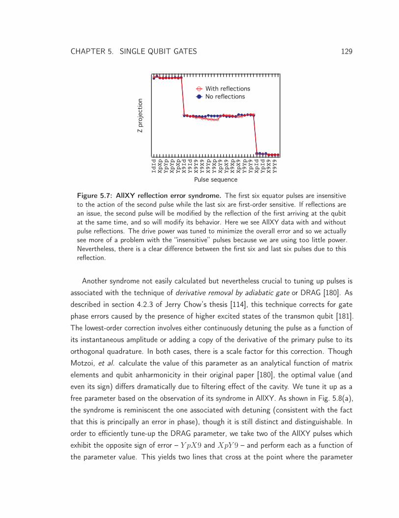
CHAPTER 5. SINGLE QUBIT GATES 129
IdId
XpXp
YpYp
XpYp
YpXp
X9Id
Y9Id
X9Y9
Y9X9
X9Yp
Y9Xp
XpY9
YpX9
X9Xp
XpX9
Y9Yp
YpY9
XpId
YpId
X9X9
Y9Y9
Figure 5.7: AllXY reflection error syndrome. The first six equator pulses are insensitiveto the action of the second pulse while the last six are first-order sensitive. If reflections arean issue, the second pulse will be modified by the reflection of the first arriving at the qubitat the same time, and so will modify its behavior. Here we see AllXY data with and withoutpulse reflections. The drive power was tuned to minimize the overall error and so we actuallysee more of a problem with the “insensitive” pulses because we are using too little power.Nevertheless, there is a clear difference between the first six and last six pulses due to thisreflection.
Another syndrome not easily calculated but nevertheless crucial to tuning up pulses isassociated with the technique of derivative removal by adiabatic gate or DRAG [180]. Asdescribed in section 4.2.3 of Jerry Chow’s thesis [114], this technique corrects for gatephase errors caused by the presence of higher excited states of the transmon qubit [181].The lowest-order correction involves either continuously detuning the pulse as a function ofits instantaneous amplitude or adding a copy of the derivative of the primary pulse to itsorthogonal quadrature. In both cases, there is a scale factor for this correction. ThoughMotzoi, et al. calculate the value of this parameter as an analytical function of matrixelements and qubit anharmonicity in their original paper [180], the optimal value (andeven its sign) differs dramatically due to filtering effect of the cavity. We tune it up as afree parameter based on the observation of its syndrome in AllXY. As shown in Fig. 5.8(a),the syndrome is reminiscent the one associated with detuning (consistent with the factthat this is principally an error in phase), though it is still distinct and distinguishable. Inorder to efficiently tune-up the DRAG parameter, we take two of the AllXY pulses whichexhibit the opposite sign of error – Y pX9 and XpY 9 – and perform each as a function ofthe parameter value. This yields two lines that cross at the point where the parameter
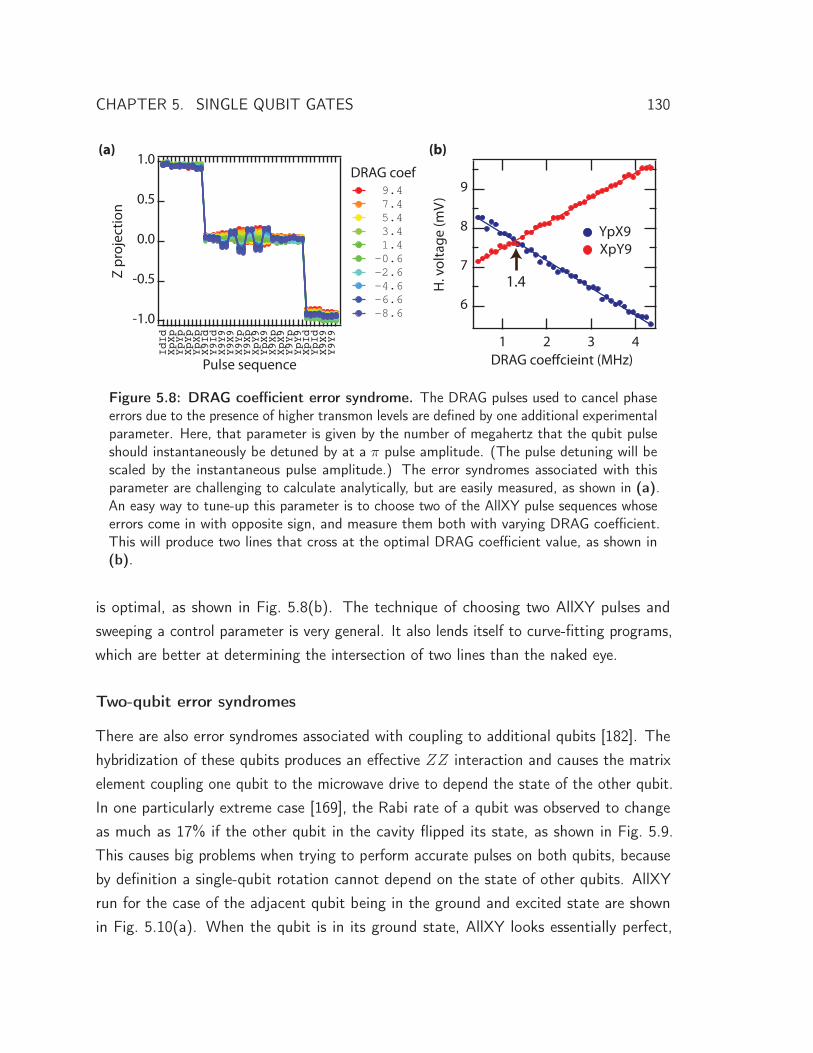
CHAPTER 5. SINGLE QUBIT GATES 130
IdId
XpXp
YpYp
XpYp
YpXp
X9Id
Y9Id
X9Y9
Y9X9
X9Yp
Y9Xp
XpY9
YpX9
X9Xp
XpX9
Y9Yp
YpY9
XpId
YpId
X9X9
Y9Y9
Pulse sequence
-1.0
-0.5
0.0
0.5
1.0
Z pr
ojec
tion
DRAG coef 9.4 7.4 5.4 3.4 1.4 -0.6 -2.6 -4.6 -6.6 -8.6
9
8
7
6
H. v
olta
ge (m
V)
4321DRAG coeffcieint (MHz)
YpX9 XpY9
(a) (b)
1.4
Figure 5.8: DRAG coefficient error syndrome. The DRAG pulses used to cancel phaseerrors due to the presence of higher transmon levels are defined by one additional experimentalparameter. Here, that parameter is given by the number of megahertz that the qubit pulseshould instantaneously be detuned by at a π pulse amplitude. (The pulse detuning will bescaled by the instantaneous pulse amplitude.) The error syndromes associated with thisparameter are challenging to calculate analytically, but are easily measured, as shown in (a).An easy way to tune-up this parameter is to choose two of the AllXY pulse sequences whoseerrors come in with opposite sign, and measure them both with varying DRAG coefficient.This will produce two lines that cross at the optimal DRAG coefficient value, as shown in(b).
is optimal, as shown in Fig. 5.8(b). The technique of choosing two AllXY pulses andsweeping a control parameter is very general. It also lends itself to curve-fitting programs,which are better at determining the intersection of two lines than the naked eye.
Two-qubit error syndromes
There are also error syndromes associated with coupling to additional qubits [182]. Thehybridization of these qubits produces an effective ZZ interaction and causes the matrixelement coupling one qubit to the microwave drive to depend the state of the other qubit.In one particularly extreme case [169], the Rabi rate of a qubit was observed to changeas much as 17% if the other qubit in the cavity flipped its state, as shown in Fig. 5.9.This causes big problems when trying to perform accurate pulses on both qubits, becauseby definition a single-qubit rotation cannot depend on the state of other qubits. AllXYrun for the case of the adjacent qubit being in the ground and excited state are shownin Fig. 5.10(a). When the qubit is in its ground state, AllXY looks essentially perfect,
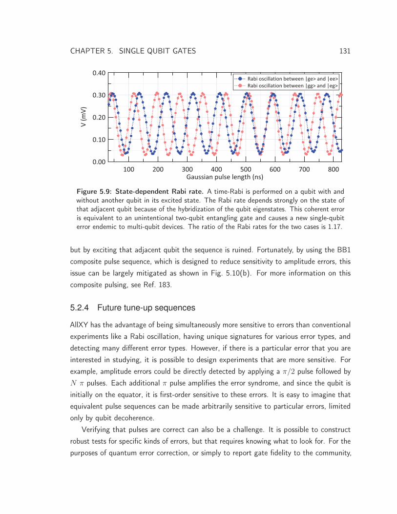
CHAPTER 5. SINGLE QUBIT GATES 131
Figure 5.9: State-dependent Rabi rate. A time-Rabi is performed on a qubit with andwithout another qubit in its excited state. The Rabi rate depends strongly on the state ofthat adjacent qubit because of the hybridization of the qubit eigenstates. This coherent erroris equivalent to an unintentional two-qubit entangling gate and causes a new single-qubiterror endemic to multi-qubit devices. The ratio of the Rabi rates for the two cases is 1.17.
but by exciting that adjacent qubit the sequence is ruined. Fortunately, by using the BB1composite pulse sequence, which is designed to reduce sensitivity to amplitude errors, thisissue can be largely mitigated as shown in Fig. 5.10(b). For more information on thiscomposite pulsing, see Ref. 183.
5.2.4 Future tune-up sequences
AllXY has the advantage of being simultaneously more sensitive to errors than conventionalexperiments like a Rabi oscillation, having unique signatures for various error types, anddetecting many different error types. However, if there is a particular error that you areinterested in studying, it is possible to design experiments that are more sensitive. Forexample, amplitude errors could be directly detected by applying a π/2 pulse followed byN π pulses. Each additional π pulse amplifies the error syndrome, and since the qubit isinitially on the equator, it is first-order sensitive to these errors. It is easy to imagine thatequivalent pulse sequences can be made arbitrarily sensitive to particular errors, limitedonly by qubit decoherence.
Verifying that pulses are correct can also be a challenge. It is possible to constructrobust tests for specific kinds of errors, but that requires knowing what to look for. For thepurposes of quantum error correction, or simply to report gate fidelity to the community,
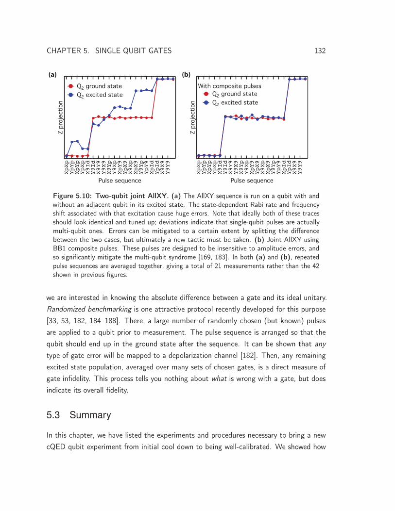
CHAPTER 5. SINGLE QUBIT GATES 132
Z pr
ojec
tion
XpXp
YpYp
XpYp
YpXp
X9Id
Y9Id
X9Y9
Y9X9
X9Yp
Y9Xp
XpY9
YpX9
X9Xp
XpX9
Y9Yp
YpY9
XpId
YpId
X9X9
Y9Y9
Pulse sequence
With composite pulses Q2 ground state Q2 excited state
Z pr
ojec
tion
XpXp
YpYp
XpYp
YpXp
X9Id
Y9Id
X9Y9
Y9X9
X9Yp
Y9Xp
XpY9
YpX9
X9Xp
XpX9
Y9Yp
YpY9
XpId
YpId
X9X9
Y9Y9
Pulse sequence
Q2 ground state Q2 excited state
(a) (b)
Figure 5.10: Two-qubit joint AllXY. (a) The AllXY sequence is run on a qubit with andwithout an adjacent qubit in its excited state. The state-dependent Rabi rate and frequencyshift associated with that excitation cause huge errors. Note that ideally both of these tracesshould look identical and tuned up; deviations indicate that single-qubit pulses are actuallymulti-qubit ones. Errors can be mitigated to a certain extent by splitting the differencebetween the two cases, but ultimately a new tactic must be taken. (b) Joint AllXY usingBB1 composite pulses. These pulses are designed to be insensitive to amplitude errors, andso significantly mitigate the multi-qubit syndrome [169, 183]. In both (a) and (b), repeatedpulse sequences are averaged together, giving a total of 21 measurements rather than the 42shown in previous figures.
we are interested in knowing the absolute difference between a gate and its ideal unitary.Randomized benchmarking is one attractive protocol recently developed for this purpose[33, 53, 182, 184–188]. There, a large number of randomly chosen (but known) pulsesare applied to a qubit prior to measurement. The pulse sequence is arranged so that thequbit should end up in the ground state after the sequence. It can be shown that anytype of gate error will be mapped to a depolarization channel [182]. Then, any remainingexcited state population, averaged over many sets of chosen gates, is a direct measure ofgate infidelity. This process tells you nothing about what is wrong with a gate, but doesindicate its overall fidelity.
5.3 Summary
In this chapter, we have listed the experiments and procedures necessary to bring a newcQED qubit experiment from initial cool down to being well-calibrated. We showed how

CHAPTER 5. SINGLE QUBIT GATES 133
to measure the cavity frequency with a transmission measurement, and how measuringtransmission as a function of drive power can quickly detect the presence and approximatedetuning of a qubit. With the measurement set up, the qubit can be found by usingspectroscopy. Of the several variants, by far the most common and conceptually simpleversion is pulsed spectroscopy. With the qubit found, we can then go about tuning upsingle-qubit rotations. Gross calibrations are done with Rabi and Ramsey oscillations toget the pulse power and qubit frequency correct, respectively. We have developed a moresophisticated sequence known as AllXY which is both more sensitive to detuning and pulsepower and detects numerous other error syndromes that the earlier sequences cannot.However, if you are interested in tuning up a particular pulse parameter, there are otherprotocols that can be made much more sensitive than AllXY by concatenating multiplerotations together. Quantifying the fidelity of pulses is challenging, but one promisingapproach is to use randomized benchmarking. In the next chapter, we will discuss ingreater detail the various measurement schemes that we previously alluded to.

CHAPTER 6
Qubit Measurement
The measurement of qubits has been a major line of research for the last several years,both for the field in general and this thesis specifically. Broadly speaking, quantum
measurement involves entangling a qubit with some other degree of freedom which canbe measured to infer the qubit state. Measuring the pointer state of our ancillary degreeof freedom projects the qubit along some axis, which is usually defined to be the qubitz-axis. In cQED, the extra degree of freedom is the cavity and the pointer state is itsdisplacement. The fundamental mechanism for measurement in cQED is shown in thedispersive Jaynes-Cummings Hamiltonian (section 3.2.3). There, the cavity frequencydepends on the state of the qubit, so driving the cavity entangles the cavity and qubitstates since the cavity displacement depends on the detuning of the drive. This physicsis straightforward in principle, but we will see that optimizing readout, when faced withexperimental realities, can be subtle and complicated.
There are three main sections to this chapter. The first introduces the experimentaluse of the low-power dispersive measurement (see section 3.2.3). There, we apply a weaktone to the cavity and measure the resulting transmission. Since the cavity displacementdepends on the qubit due to the dispersive coupling, the amount of transmitted lightsimilarly encodes the qubit state. When used with a conventional microwave amplifier,however, and especially in experiments that do not explicitly optimize system parameters for
135
CHAPTER 6. QUBIT MEASUREMENT 136
measurement, the resulting fidelity can be low. The situation has improved recently with thedevelopment of practical quantum-limited microwave amplifiers which dramatically reduceadded noise at the cost of increased complexity. This section will introduce experimentalquantum measurement in cQED, and will provide much of the language and intuition usedlater.
The second section seeks to optimize the fidelity of the dispersive readout. As wewill see, under normal circumstances the qubit and cavity lifetimes are interrelated by thePurcell effect. This inhibits our ability to increase measurement fidelity by independentlyoptimizing those lifetimes. In response, we introduce the Purcell filter, which breaks (or atleast, engineers improvements in) the relationship between the qubit and cavity lifetime. Itcan significantly increase qubit lifetime and therefore dispersive measurement fidelity, andhas the advantage of being compatible with quantum-limited amplifiers. As an ancillarybenefit, we will discover that the Purcell filter can also enable efficient reset of the qubitby swapping long-lived qubit excitations into the short-lived cavity mode.
The third and final section concerns an unexpected behavior which was accidentallydiscovered when measuring the first Purcell filter device. As a function of drive strength,cavity transmission initially looks linear and lorentzian at low drive strengths but rapidlydevelops anharmonic behavior as the inherited qubit nonlinearity comes into play withhigher excitations. It was long thought that these nonlinearities, which eliminate readoutcontrast, set the maximum drive strength that could be used to measure. However, we findthat if you drive even harder, the cavity eventually restores to a linear lorentzian responseat a different frequency. The power required to reach this bright state depends on theinitial qubit state, providing what turns out to be a very high fidelity qubit measurementthat is not affected by following amplifier noise. While this mechanism works well for awide range in qubit and cavity parameters, it scrambles the qubit and cavity state (e.g. isnot quantum non-demolition) and is not applicable to some experiments.
6.1 Dispersive readout
We saw in section 3.2.3 that, in the dispersive limit, the Jaynes-Cummings Hamiltoniansimplifies to
H = �ωra†a+ �
ωq
2σz + �χa†aσz (6.1)

CHAPTER 6. QUBIT MEASUREMENT 137
where ωr is the cavity frequency, ωq the qubit frequency, and χ the dispersive shift. Recallthat the first term is responsible for the cavity oscillator (with the zero-point energyincluded, but suppressed from now on), the second responsible for the two-level qubit∗, andthe third responsible for the state-dependent frequency shift. In the case of a true two-levelqubit, χ = g2/Δ, but for transmon qubits, this parameter becomes χ = g2
Δα
Δ−α[115]. We
have already taken the rotating wave approximation, ignoring terms like a†σ+ and aσ−
which do not conserve energy, and assumed that the detuning Δ = |ωr − ωq| � g, whereg is the vacuum-Rabi splitting.
For the purposes of qubit readout, we group the dispersive term with the cavity numberoperator, giving us Hc = �a†a (ωr + χσz) (section 3.2.3). This shows that cavity frequencydepends on the qubit state; the frequency when the qubit is in the ground state is 2χ higherthan when it is in the excited state. In the case of transmon qubits, ωr is a convenientfrequency with which to write the Hamiltonian and has no physical significance. Boththe ground and excited state peaks are shifted up in frequency relative to the bare cavityfrequency, but the ground state shift is larger, by what we call 2χ. (In the Cooper-pairbox limit, the two χ shifts are actually equal and opposite, but this symmetry is broken bythe higher transmon levels.)
We can demonstrate the dispersive cavity shift with a simple pulsed transmissionexperiment. We first prepare the qubit in either its ground or excited state and thenmeasure the transmission of a short RF tone, as shown in Fig. 6.1. There, the dispersiveshift 2χ is much larger than the cavity linewidth κ, so the two cavity frequencies arewell-resolved. The qubit has some chance of decaying during the measurement, so we seea small peak in the blue curve corresponding to the qubit being in the ground state. Thismeasurement was done with a drive power small enough that the mean cavity occupationis approximately one photon so as to avoid the nonlinear cavity effects discussed insection 6.3.1.
In order to measure the qubit, we apply a tone at the ground-state cavity frequency andmeasure how much is transmitted. If we get a relatively large transmission, we can inferthat the qubit must be in the ground state, while a relatively small signal indicates thatthe qubit is excited. That is, we take advantage of a state-dependent cavity transmission.If we send a single photon of the relevant frequency through the cavity and see it come
∗ If we include higher transmon levels, we find that each has a different dispersive shift to the cavity. Itis therefore possible, if you can measure both the phase and amplitude of the transmitted signal, todiscriminate between several qubit states in a single shot [189].
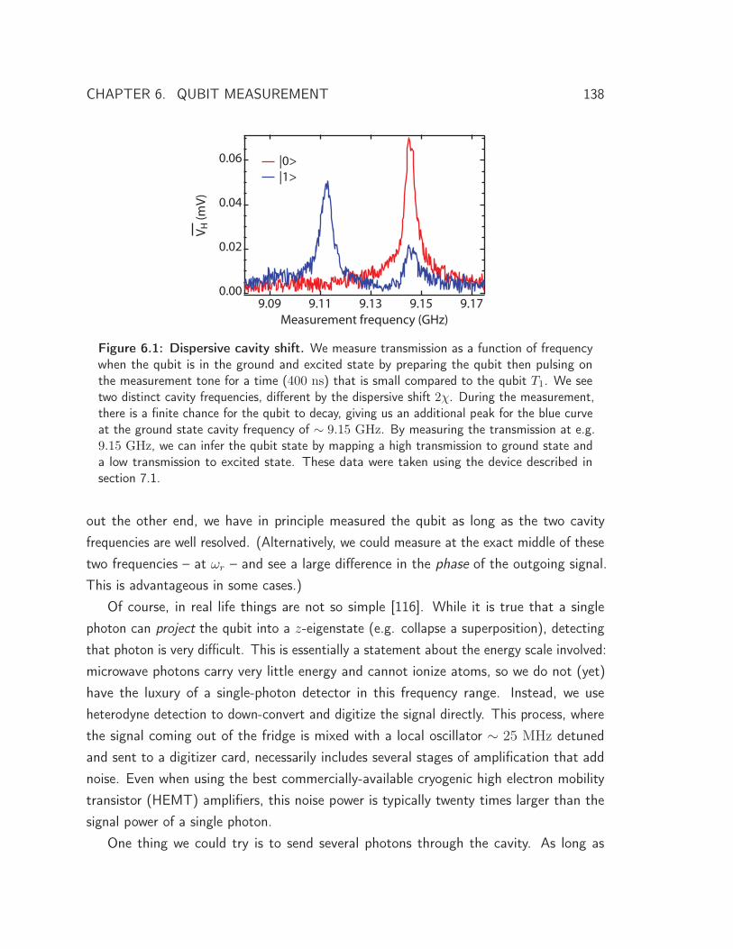
CHAPTER 6. QUBIT MEASUREMENT 138
Figure 6.1: Dispersive cavity shift. We measure transmission as a function of frequencywhen the qubit is in the ground and excited state by preparing the qubit then pulsing onthe measurement tone for a time (400 ns) that is small compared to the qubit T1. We seetwo distinct cavity frequencies, different by the dispersive shift 2χ. During the measurement,there is a finite chance for the qubit to decay, giving us an additional peak for the blue curveat the ground state cavity frequency of ∼ 9.15 GHz. By measuring the transmission at e.g.9.15 GHz, we can infer the qubit state by mapping a high transmission to ground state anda low transmission to excited state. These data were taken using the device described insection 7.1.
out the other end, we have in principle measured the qubit as long as the two cavityfrequencies are well resolved. (Alternatively, we could measure at the exact middle of thesetwo frequencies – at ωr – and see a large difference in the phase of the outgoing signal.This is advantageous in some cases.)
Of course, in real life things are not so simple [116]. While it is true that a singlephoton can project the qubit into a z-eigenstate (e.g. collapse a superposition), detectingthat photon is very difficult. This is essentially a statement about the energy scale involved:microwave photons carry very little energy and cannot ionize atoms, so we do not (yet)have the luxury of a single-photon detector in this frequency range. Instead, we useheterodyne detection to down-convert and digitize the signal directly. This process, wherethe signal coming out of the fridge is mixed with a local oscillator ∼ 25 MHz detunedand sent to a digitizer card, necessarily includes several stages of amplification that addnoise. Even when using the best commercially-available cryogenic high electron mobilitytransistor (HEMT) amplifiers, this noise power is typically twenty times larger than thesignal power of a single photon.
One thing we could try is to send several photons through the cavity. As long as
CHAPTER 6. QUBIT MEASUREMENT 139
the qubit does not decay, we are free to do this because the third term in equation 6.1commutes with the the other terms. (Formally, this is because the measurement is QNDto the qubit state; when we measure the qubit, it remains in the same state in whichwe had measured it.) How much signal could we gather with this process? We mustremember that we can only send photons through the cavity as long as the qubit hasnot decayed. Since we cannot know when that has happened, we aim to integrate fora time Δt which is on the order of the T1 of the qubit. (Exactly how long you shouldmeasure turns out to be a bit complicated, and is touched on in a footnote below.) Next,the amount of information we extract per photon is not necessarily one full bit. If thedispersive shift is smaller than the cavity linewidth, for example, we will gain an amount ofinformation expressed as sin2(θ), where θ = tan−1
(2χκ
), which is bounded between 0 and
1 bit. (We get a full bit when the state-dependent shift χ is much larger than the cavitybandwidth κ.) Finally, each of these photons will give us �ωr of energy and the rate ofphoton collection is set by the bandwidth of the cavity κ. If we have 〈n〉 equilibrium cavityphotons, our information gain (in units of energy) during a measurement will be given by
Esignal = 〈n〉�ωrsin2(θ)T1κ. (6.2)
If we specify the noise of our measurement chain with an effective noise temperature TN
our signal to noise ratio is given by SNR = Esignal/kBTN .For most devices, this number turns out to be rather small. Assuming fairly favorable
numbers of a mean cavity occupation 〈n〉 = 10 photons∗, an 8 GHz measurement cavity,an integration time of 3 μs, κ = 5 MHz, and a 10 K noise temperature (typical whenusing only a HEMT), we have SNR ∼ 1. (In Cooper-pair box devices or more recent 3Dtransmon devices with longer lifetimes, this number can be more like 5 − 10.) As a result,for a conventional amplification chain, the fraction of the time you can correctly identifythe qubit state with a dispersive measurement is bounded to about 70%. For devices withparameters less favorable for dispersive measurement (e.g. a longer cavity lifetime), fidelityvalues have been observed as low as 5− 10%, though this is atypical. Robust quantumerror correction requires fidelities in excess of 99%, so this performance must be improved.
Fortunately, significant progress has recently been made in the development of spe-cialized quantum-limited amplifiers [190–192]. The idea is to put an extremely low-noise
∗ The reason we cannot just increase the number of intra-cavity photons will be discussed in section 6.3.Ten photons is approximately where cavity nonlinearity and a reduction in qubit T1 start to dominate.

CHAPTER 6. QUBIT MEASUREMENT 140
amplifier like a Josephson parametric converter (JPC) or Josephson bifurcation amplifier(JBA) between the cavity and the cryogenic commercial amplifier, so as to boost thesignal and drown out the added HEMT noise. This significantly reduces the effectiveamplification chain noise temperature, increasing SNR and measurement fidelity. Forexample, if we reduce the noise temperature to three times the quantum limit, or 100 mK,and re-calculate the signal to noise ratio with the parameters as above, we find SNR ∼ 50
(or, with state-of-the-art lifetimes, several hundred). As a result, dispersive measurementscan now resolve individual quantum jumps of the qubit state in real time [60] and areapproaching 99.5% fidelity [61]. This comes at a cost of complexity. The amplifiers haveto be biased with a very stable RF source, require extra circulators, and have narrowamplification bandwidth that must be matched with the cavity. Nevertheless, it is clearthat as the engineering challenges are overcome, the use of these devices will become moreroutine (a process which is coinciding with the writing of this thesis), enabling high fidelityQND measurement and real-time feedback. For the purposes of this chapter, however, wefocus on improvements we can make without using these special devices.
Another method to circumvent amplifier noise is to intentionally make the cavityextremely nonlinear with the addition of a Josephson junction. The cavity will then exhibita “latching” Kerr bistability between two long-lived and classically distinguishable states.The qubit state can be mapped onto the choice of cavity state and read out over a relativelylong period of time, yielding higher fidelity [193–196]. As with low-noise amplifiers, thisapproach also increases complexity of both fabrication and the physics of the device sincethe cavities require an additional junction. Though we will not further discuss this approach,it is as an interesting context for section 6.3, in which we produce a qualitatively similarbehavior without the need of an extra cavity junction.
6.2 The Purcell filter
In considering how to optimize the fidelity of dispersive readout, we quickly reach animpasse. On the one hand, we would like to have the fastest possible cavity (e.g. a large κ)to maximize the rate of measurement photon transmission; on the other hand, decreasingcavity lifetime can also reduce qubit lifetime due to the Purcell effect [139, 148]. For afixed signal to noise ratio, the optimal measurement time is a fixed fraction of T1. HigherSNRs require shorter and shorter integration times to optimize the resulting measurementfidelity [116]. The reason for this is simple: the readout is QND but the qubit is free to
CHAPTER 6. QUBIT MEASUREMENT 141
decay during the measurement. When this happens, all measurement integration followingthe decay event will actually lower the measurement faithfulness, because we are interestedin what the qubit state was at the beginning of the measurement and not what it iscurrently∗. Thus, lowering qubit T1 will lower measurement fidelity.
6.2.1 The Purcell effect
The Purcell effect modifies the lifetime of any quantized system coupled to a resonantcircuit or cavity [148]. Depending on the detuning of the system transition frequency fromthe cavity resonance frequency and the lifetime of the cavity, the rate of decay of thequantum system can be strongly enhanced [148, 197] or suppressed [198–200] relative tothe decay rate to the electromagnetic continuum. In cQED, qubits are often sufficientlydetuned to have suppressed decay rates compared with the continuum, but T1 can stillbe limited by radiative decay through the cavity. That is, the qubit decaying throughthe cavity is always a possible mode of relaxation, but it may or may not be dominantdepending on the coupling strength and cavity lifetime. When a significant fraction ofqubit relaxation is decay through the cavity, we say that the qubit is “Purcell-limited.”
We can make a rough approximation of the Purcell lifetime with the single-modeJaynes-Cummings Hamiltonian (equation 3.38). In this case, H = �ωr
(a†a+ 1
2
)+
�ωq
2σz + �g
(a†σ− + aσ+
), with g the coupling strength, ωr the cavity frequency, and ωq
the qubit frequency. Using first-order non-degenerate perturbation theory (expanding inpowers of g
Δ), we find that the dressed qubit-like eigenstate of the system is given by
|dressed〉 ≈ |e, 0〉 + gΔ|g, 1〉 (see Appendix B of David Schuster’s thesis [112]). There,
|e, 0〉 is the undressed eigenstate of an excited qubit and zero photons, |g, 1〉 is the
∗ The optimal length of integration is complicated by the possibility of both linear and nonlinear filtering.One example of linear filtering is to multiply the measurement tone by an exponential decay. The data atthe beginning of the measurement will then count for more than that of later measurements, amelioratingthe effect of finite qubit lifetime. Indeed, such a filter can improve with low SNRs, though its effectivenessdrops rapidly for larger SNRs [116].
Processing data in real time with a nonlinear filter can do even better if you have knowledge of thedistribution of measurement outcomes as a function of integration time [61]. For example, if, shortly afterthe measurement is started, the integrated homodyne voltage is already located far down one of the tailsof the “S-curve” distribution, then you already know with high confidence what the qubit state was andthe measurement is complete.
In the case of the simple boxcar integration of the measurement tone that is used in most experiments,the x% of T1 integration time for 1-x fidelity rule of thumb is a good approximation. That is, in order toget 99% measurement fidelity, you need high enough SNR to accurately read out the qubit within nomore than 1% of T1.

CHAPTER 6. QUBIT MEASUREMENT 142
10-1
100
101
102
103
104
105
T 1 (μ
s)
2015105Frequency (GHz)
Single-mode Purcell Multi-mode Purcell
Figure 6.2: Multi-mode vs single-mode Purcell decay rates. We calculate the Purcelllifetime for a single mode with T−1
1 = γκ = (g/Δ)2κ for a device with g = 300 MHz. Weconsider a symmetric device where Cin = Cout = 1 fF. We use the relation qi = ωCiZ0,κi =
(2π
)q2i ω and κ = κin + κout. Qtot = 124, 000. We compare this to a multi-mode
circuit model using a transmission line of length l = 7650 μm, an impedance Z0 = 50 Ω, acapacitive qubit coupling Cc = 20 fF and a qubit capacitance Cq = 55 fF. In both cases,the resonance frequency of the cavity is 8.02 GHz. Note the significant difference betweenthe two predictions when substantially detuned from the first cavity resonance.
undressed qubit in the ground state and one photon, and Δ the qubit-cavity detuning (seesection 3.2.2). We can then say that the Purcell decay rate is given by the decay of thephoton-like component of this state at the cavity decay rate κ, γκ =
(gΔ
)2κ.
This is an excellent approximation for the case of a single-mode cavity. However, weare coupling to a transmission line or 3D cavity that has many independent spatial modeswhich can also couple strongly to and induce decay of the qubit [139]. As a result, whenthe qubit is appreciably detuned from any particular mode, the single-mode approximationis very poor, as shown in Fig. 6.2. To correctly calculate the Purcell effect, we mustincorporate the full impedance environment seen by the qubit. As explained in section 3.3.2,the relationship between qubit T1 due to spontaneous emission and admittance Y of thecoupled environment is
TPurcell1 =
Cq
Re[Y (ωq)], (6.3)
where Cq is the qubit capacitance [Fig. 6.3(a)] [150, 151]. This equation, which isequivalent to Fermi’s golden rule, has previously been used to accurately model TPurcell
1
when all modes of the cavity are taken into account in the calculation of Y [139] and the
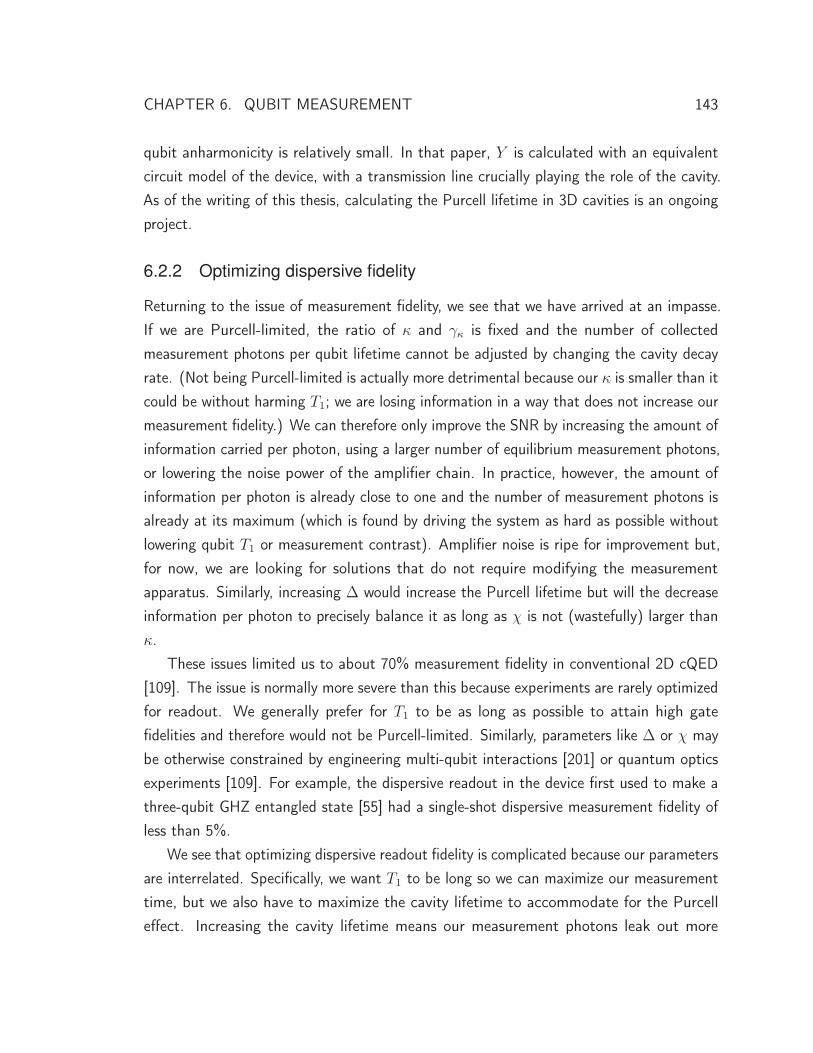
CHAPTER 6. QUBIT MEASUREMENT 143
qubit anharmonicity is relatively small. In that paper, Y is calculated with an equivalentcircuit model of the device, with a transmission line crucially playing the role of the cavity.As of the writing of this thesis, calculating the Purcell lifetime in 3D cavities is an ongoingproject.
6.2.2 Optimizing dispersive fidelity
Returning to the issue of measurement fidelity, we see that we have arrived at an impasse.If we are Purcell-limited, the ratio of κ and γκ is fixed and the number of collectedmeasurement photons per qubit lifetime cannot be adjusted by changing the cavity decayrate. (Not being Purcell-limited is actually more detrimental because our κ is smaller than itcould be without harming T1; we are losing information in a way that does not increase ourmeasurement fidelity.) We can therefore only improve the SNR by increasing the amount ofinformation carried per photon, using a larger number of equilibrium measurement photons,or lowering the noise power of the amplifier chain. In practice, however, the amount ofinformation per photon is already close to one and the number of measurement photons isalready at its maximum (which is found by driving the system as hard as possible withoutlowering qubit T1 or measurement contrast). Amplifier noise is ripe for improvement but,for now, we are looking for solutions that do not require modifying the measurementapparatus. Similarly, increasing Δ would increase the Purcell lifetime but will the decreaseinformation per photon to precisely balance it as long as χ is not (wastefully) larger thanκ.
These issues limited us to about 70% measurement fidelity in conventional 2D cQED[109]. The issue is normally more severe than this because experiments are rarely optimizedfor readout. We generally prefer for T1 to be as long as possible to attain high gatefidelities and therefore would not be Purcell-limited. Similarly, parameters like Δ or χ maybe otherwise constrained by engineering multi-qubit interactions [201] or quantum opticsexperiments [109]. For example, the dispersive readout in the device first used to make athree-qubit GHZ entangled state [55] had a single-shot dispersive measurement fidelity ofless than 5%.
We see that optimizing dispersive readout fidelity is complicated because our parametersare interrelated. Specifically, we want T1 to be long so we can maximize our measurementtime, but we also have to maximize the cavity lifetime to accommodate for the Purcelleffect. Increasing the cavity lifetime means our measurement photons leak out more
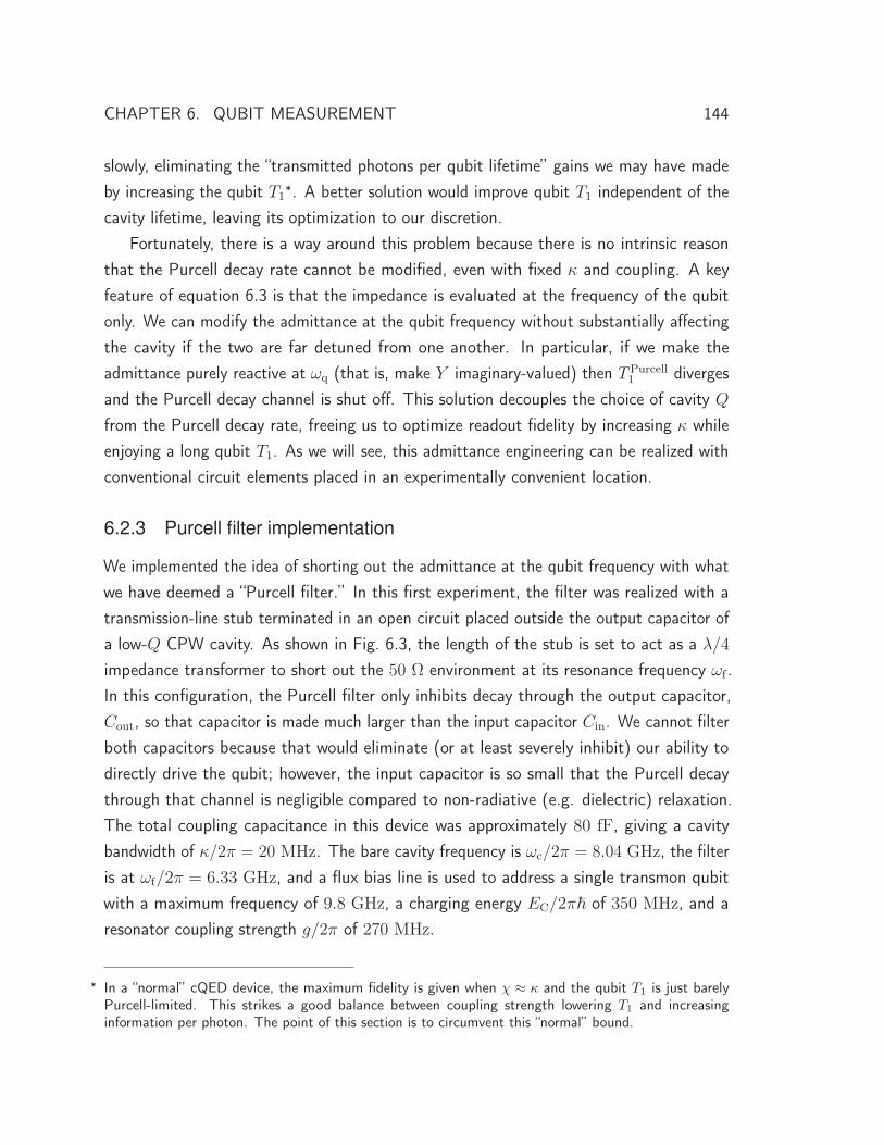
CHAPTER 6. QUBIT MEASUREMENT 144
slowly, eliminating the “transmitted photons per qubit lifetime” gains we may have madeby increasing the qubit T1
∗. A better solution would improve qubit T1 independent of thecavity lifetime, leaving its optimization to our discretion.
Fortunately, there is a way around this problem because there is no intrinsic reasonthat the Purcell decay rate cannot be modified, even with fixed κ and coupling. A keyfeature of equation 6.3 is that the impedance is evaluated at the frequency of the qubitonly. We can modify the admittance at the qubit frequency without substantially affectingthe cavity if the two are far detuned from one another. In particular, if we make theadmittance purely reactive at ωq (that is, make Y imaginary-valued) then TPurcell
1 divergesand the Purcell decay channel is shut off. This solution decouples the choice of cavity Q
from the Purcell decay rate, freeing us to optimize readout fidelity by increasing κ whileenjoying a long qubit T1. As we will see, this admittance engineering can be realized withconventional circuit elements placed in an experimentally convenient location.
6.2.3 Purcell filter implementation
We implemented the idea of shorting out the admittance at the qubit frequency with whatwe have deemed a “Purcell filter.” In this first experiment, the filter was realized with atransmission-line stub terminated in an open circuit placed outside the output capacitor ofa low-Q CPW cavity. As shown in Fig. 6.3, the length of the stub is set to act as a λ/4
impedance transformer to short out the 50 Ω environment at its resonance frequency ωf .In this configuration, the Purcell filter only inhibits decay through the output capacitor,Cout, so that capacitor is made much larger than the input capacitor Cin. We cannot filterboth capacitors because that would eliminate (or at least severely inhibit) our ability todirectly drive the qubit; however, the input capacitor is so small that the Purcell decaythrough that channel is negligible compared to non-radiative (e.g. dielectric) relaxation.The total coupling capacitance in this device was approximately 80 fF, giving a cavitybandwidth of κ/2π = 20 MHz. The bare cavity frequency is ωc/2π = 8.04 GHz, the filteris at ωf/2π = 6.33 GHz, and a flux bias line is used to address a single transmon qubitwith a maximum frequency of 9.8 GHz, a charging energy EC/2π� of 350 MHz, and aresonator coupling strength g/2π of 270 MHz.
∗ In a “normal” cQED device, the maximum fidelity is given when χ ≈ κ and the qubit T1 is just barelyPurcell-limited. This strikes a good balance between coupling strength lowering T1 and increasinginformation per photon. The point of this section is to circumvent this “normal” bound.
CHAPTER 6. QUBIT MEASUREMENT 145
Figure 6.3: Design and realization of the Purcell filter. (a) Circuit model of thePurcell-filtered cavity design. The Purcell filter, implemented with λ/4 open-circuitedtransmission-line stubs, inhibits decay through Cout near its resonance ωf . We use twoidentical stubs above and below the major axis of the chip to maximize the symmetry of thedevice, in an effort to suppress undesired on-chip resonances. A flux bias line is includedto tune the frequency of the qubit in-situ by changing the magnetic flux through the qubitSQUID loop. (b) Optical micrograph of the device with inset zoom on transmon qubit. Notethe correspondence of the circuit elements directly above in (a). The device is made withstandard 2D cQED fabrication techniques: the resonator and filter structure are niobiumpatterned on a sapphire substrate, while the single transmon qubit (shown in the inset, topleft) is fabricated using standard shadow masked double-angle aluminum deposition. Thedevice is 2 by 7 mm and is wire-bonded to a copper PC board and cooled in a standardoctobox sample holder in a helium dilution fridge. (Figure used with permission from [143].See Copyright Permissions.)
CHAPTER 6. QUBIT MEASUREMENT 146
Figure 6.4: Diagnostic transmission data of the Purcell filter. We measured transmis-sion through the Purcell-filtered cavity at 4.2 K. At ωf (arrow) the Purcell filter shorts outthe 50 Ω output environment, producing a 30 dB drop in transmission. The high frequencyoscillations visible are due to a small impedance mismatch along the measurement cables. Acircuit model incorporating only the experimental parameters Cin, Cout, ωc, and ωf showsexcellent correspondence. This gives us confidence our design and understanding of thePurcell filter. (Figure used with permission from [143]. See Copyright Permissions.)
It is worth emphasizing that the concept of a Purcell filter does not imply a particularimplementation. One might consider any structure that additionally modifies the impedanceenvironment of a cavity for the purposes of reducing the Purcell decay rate of a subsystemto be a filter. Indeed, a waveguide below cutoff has recently been constructed for use witha 3D cavity [202].
We can verify that our device is working as expected by first measuring transmissionat 4.2 K (below the superconducting transition temperature of the Niobium resonator)and comparing it with the circuit model used in design. As seen in Fig. 6.4, there is a dipcorresponding to inhibited decay through Cout at ωf . A circuit model accurately predictsthis dip and the overall structure of the transmission. The model only misses the highfrequency oscillations that are due to slight impedance mismatches (e.g. reflections) inthe measurement chain. The model used four input parameters: the input and outputcapacitance (which were simulated with the ANSYS Maxwell software package) and thefrequencies of the cavity and filter (free parameters based on the measurement), lendingconfidence to our ability to predict and engineer the impedance of the structure.
Finally, to demonstrate the filtering effect, we measured the qubit T1 as function of
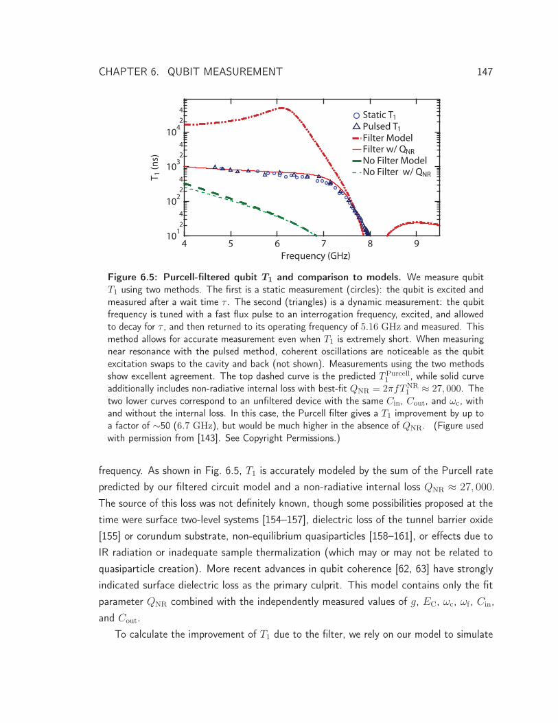
CHAPTER 6. QUBIT MEASUREMENT 147
Figure 6.5: Purcell-filtered qubit T1 and comparison to models. We measure qubitT1 using two methods. The first is a static measurement (circles): the qubit is excited andmeasured after a wait time τ . The second (triangles) is a dynamic measurement: the qubitfrequency is tuned with a fast flux pulse to an interrogation frequency, excited, and allowedto decay for τ , and then returned to its operating frequency of 5.16 GHz and measured. Thismethod allows for accurate measurement even when T1 is extremely short. When measuringnear resonance with the pulsed method, coherent oscillations are noticeable as the qubitexcitation swaps to the cavity and back (not shown). Measurements using the two methodsshow excellent agreement. The top dashed curve is the predicted TPurcell
1 , while solid curveadditionally includes non-radiative internal loss with best-fit QNR = 2πfTNR
1 ≈ 27, 000. Thetwo lower curves correspond to an unfiltered device with the same Cin, Cout, and ωc, withand without the internal loss. In this case, the Purcell filter gives a T1 improvement by up toa factor of ∼50 (6.7 GHz), but would be much higher in the absence of QNR. (Figure usedwith permission from [143]. See Copyright Permissions.)
frequency. As shown in Fig. 6.5, T1 is accurately modeled by the sum of the Purcell ratepredicted by our filtered circuit model and a non-radiative internal loss QNR ≈ 27, 000.The source of this loss was not definitely known, though some possibilities proposed at thetime were surface two-level systems [154–157], dielectric loss of the tunnel barrier oxide[155] or corundum substrate, non-equilibrium quasiparticles [158–161], or effects due toIR radiation or inadequate sample thermalization (which may or may not be related toquasiparticle creation). More recent advances in qubit coherence [62, 63] have stronglyindicated surface dielectric loss as the primary culprit. This model contains only the fitparameter QNR combined with the independently measured values of g, EC, ωc, ωf , Cin,and Cout.
To calculate the improvement of T1 due to the filter, we rely on our model to simulate
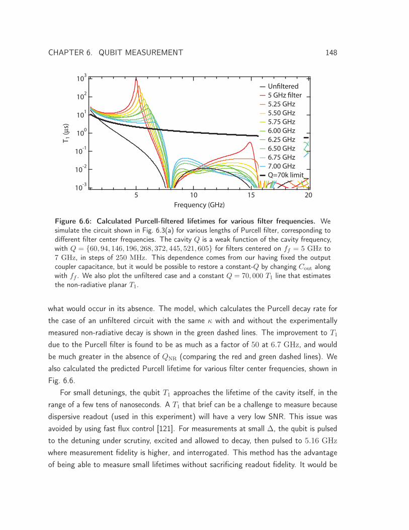
CHAPTER 6. QUBIT MEASUREMENT 148
10-3
10-2
10-1
100
101
102
103
T 1 (μ
s)
2015105Frequency (GHz)
Unfiltered 5 GHz filter 5.25 GHz 5.50 GHz 5.75 GHz 6.00 GHz 6.25 GHz 6.50 GHz 6.75 GHz 7.00 GHz Q=70k limit
Figure 6.6: Calculated Purcell-filtered lifetimes for various filter frequencies. Wesimulate the circuit shown in Fig. 6.3(a) for various lengths of Purcell filter, corresponding todifferent filter center frequencies. The cavity Q is a weak function of the cavity frequency,with Q = {60, 94, 146, 196, 268, 372, 445, 521, 605} for filters centered on ff = 5 GHz to7 GHz, in steps of 250 MHz. This dependence comes from our having fixed the outputcoupler capacitance, but it would be possible to restore a constant-Q by changing Cout alongwith ff . We also plot the unfiltered case and a constant Q = 70, 000 T1 line that estimatesthe non-radiative planar T1.
what would occur in its absence. The model, which calculates the Purcell decay rate forthe case of an unfiltered circuit with the same κ with and without the experimentallymeasured non-radiative decay is shown in the green dashed lines. The improvement to T1
due to the Purcell filter is found to be as much as a factor of 50 at 6.7 GHz, and wouldbe much greater in the absence of QNR (comparing the red and green dashed lines). Wealso calculated the predicted Purcell lifetime for various filter center frequencies, shown inFig. 6.6.
For small detunings, the qubit T1 approaches the lifetime of the cavity itself, in therange of a few tens of nanoseconds. A T1 that brief can be a challenge to measure becausedispersive readout (used in this experiment) will have a very low SNR. This issue wasavoided by using fast flux control [121]. For measurements at small Δ, the qubit is pulsedto the detuning under scrutiny, excited and allowed to decay, then pulsed to 5.16 GHz
where measurement fidelity is higher, and interrogated. This method has the advantageof being able to measure small lifetimes without sacrificing readout fidelity. It would be
CHAPTER 6. QUBIT MEASUREMENT 149
easier to pulse the qubit at the home position and only then flux it because the qubit pulsefrequency would be fixed, but the prescribed order also verifies that the qubit frequency ata given flux amplitude is truly known.
6.2.4 Qubit reset
One consequence of the Purcell filter is that the device exhibits an exceptionally largedynamic range in T1. We realize about a factor of 80 between the longest and shortesttimes measured (a ratio that would be significantly larger if not for QNR). This can beviewed as a major ancillary benefit, one so substantial that it might be advertised asenabling the primary application of the Purcell filter. That benefit is for qubit reset. As wehave already seen with the example of measurement-free [203] quantum error correction(section 2.3.4), there are many applications that benefit from or require on-demand resetof qubit state. Experimental repetition rates can be greatly enhanced when they areotherwise limited by T1. At the end of a calculation, our qubit state will in general be insome unknown superposition of its ground and excited state. If we want to do anothercalculation, we need to restore the qubit state unconditionally to some known state. Thisis normally done by waiting for the qubit to decay back to the ground state at a rate1/T1. As qubit lifetimes increase [62], this can be inconveniently slow. Resetting the qubitwould greatly increase experimental bandwidth. Similarly, experiments that use a qubit tomake repeated measurements of a coupled system also require resetting the qubit betweeninterrogations [109].
With our Purcell filtered device, we can exploit the sudden drop in qubit lifetime inthe vicinity of the cavity to perform reset. We normally operate far detuned from thecavity, where the qubit T1 is not Purcell-limited. To reset, we can quickly move the qubitfrequency near resonance with the cavity using a fast flux pulse. The qubit excitationis dumped into the cavity and quickly decays to the environment∗. Though this couldwork for any flux-tunable cQED device, the Purcell filter greatly improves the flexibility ofthis process. It can exhibit a dramatically increased “lifetime contrast” – the ratio of thelongest to shortest qubit T1 – through the use of a low-Q cavity that does not limit qubitT1 at its operating frequency. This concept has been used in other experiments, but byresetting through a spurious lossy two-level system that couples to the qubit rather thanan engineered cavity mode [204].
∗ It is worth noting that reseting with the Purcell filter need not require fast flux tunability. There are
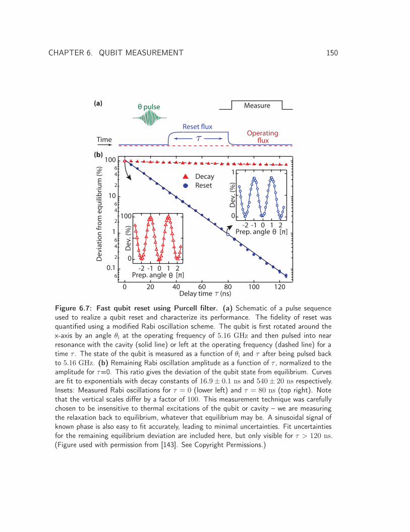
CHAPTER 6. QUBIT MEASUREMENT 150
τ
(a)
(b)
Time
Measureθ pulse
Reset fluxOperating
flux
θ
θ
Figure 6.7: Fast qubit reset using Purcell filter. (a) Schematic of a pulse sequenceused to realize a qubit reset and characterize its performance. The fidelity of reset wasquantified using a modified Rabi oscillation scheme. The qubit is first rotated around thex-axis by an angle θi at the operating frequency of 5.16 GHz and then pulsed into nearresonance with the cavity (solid line) or left at the operating frequency (dashed line) for atime τ . The state of the qubit is measured as a function of θi and τ after being pulsed backto 5.16 GHz. (b) Remaining Rabi oscillation amplitude as a function of τ , normalized to theamplitude for τ=0. This ratio gives the deviation of the qubit state from equilibrium. Curvesare fit to exponentials with decay constants of 16.9± 0.1 ns and 540± 20 ns respectively.Insets: Measured Rabi oscillations for τ = 0 (lower left) and τ = 80 ns (top right). Notethat the vertical scales differ by a factor of 100. This measurement technique was carefullychosen to be insensitive to thermal excitations of the qubit or cavity – we are measuringthe relaxation back to equilibrium, whatever that equilibrium may be. A sinusoidal signal ofknown phase is also easy to fit accurately, leading to minimal uncertainties. Fit uncertaintiesfor the remaining equilibrium deviation are included here, but only visible for τ > 120 ns.(Figure used with permission from [143]. See Copyright Permissions.)
CHAPTER 6. QUBIT MEASUREMENT 151
The efficacy of reset in this device is readily quantified using a modified Rabi oscillationsequence. As shown in Fig. 6.7(a), the qubit is rotated by some angle and then resetfor some time before being measured. The amplitude of the remaining sinusoidal Rabioscillation indicates the degree to which the qubit is out of equilibrium after the reset timeτ . The protocol was chosen so as to be insensitive to any equilibrium thermal populationof the qubit. The non-equilibrium population is found to exhibit pure exponential decayover three orders of magnitude. The qubit can be reset to 99.9% in 120 ns or any otherfidelity depending on τ (e.g. 99% for 80 ns or one “9” every 40 ns). The sequence isalso performed with the qubit remaining at the operating frequency during the delay todemonstrate the large dynamic range of T1 available in this system. The dynamic rangewould be much higher in the absence of the non-radiative QNR limiting qubit lifetimes towell below the Purcell limit when far detuned.
One potential concern with using this technique in larger systems is what would happenwere we to reset one qubit by transferring its population into the cavity, which is itselfcoupled to other qubits. This photon would cause a χ shift on all the others, and since thedecay of that excitation out of the cavity is stochastic (e.g. the time it takes to decay, andtherefore the phase it evolves, is random), would result in dephasing of all the other qubits[144]. This could be avoided by either turning off the χs of the other cavities by detuningthem or by using separate reset cavities for each qubit. Having separate cavities mightseem a bit extravagant, but it should not be any more costly (and it could potentiallybe much more useful) than a flux bias line per qubit. This is especially attractive givenrecent methods of entangling subsets of qubits with all-microwave drives [169, 176, 209]which may eliminate the need for flux bias lines. This extra cavity mode could also beimplemented for individual qubit readout, a functionality that fulfills one of the DiVincenzocriteria (section 2.2.2).
several methods of unconditionally swapping excitations from the qubit into the cavity [205–207], butthey all benefit from a large dynamic range between cavity and qubit lifetimes. We need some non-unitaryevolution to reset the qubit, which can be granted by the cavity decay. Another possible non-unitaryinitialization is to measure the qubit and use that classical information to feed back and set the state[172, 208]. This has the advantage of being something that we will need to do anyway in a “real” quantumcomputer, giving us initialization essentially for free.
CHAPTER 6. QUBIT MEASUREMENT 152
6.2.5 Purcell filter summary
The Purcell filter seeks to solve the problem of radiative decay of the qubit through thecavity to which it is coupled. We approached this problem in the context of measurementfidelity, but it should be understood as a general problem of maximizing qubit coherencewhen coupled to a lossy external impedance (section 3.3.2). One can always reducecoupling or increase cavity lifetime, but doing so will have unwelcome implications formeasurement fidelity. Fortunately, there is no reason that the qubit needs to decay througha coupled cavity at all. As long as the frequencies of the respective modes are sufficientlydetuned, the cavity and qubit sample distinct impedance environments. We exploited thisfact by creating a Purcell filter using a piece of shorted transmission line. This objectshorts out the coupled environment at the qubit frequency while minimally changing it atthe cavity frequency. The resulting device demonstrated that the Purcell effect was shutoff in accordance with our expectations and also exhibited a very large dynamic range inqubit T1. Combining this resource with fast flux, we showed the ability to reset our qubitback to equilibrium very rapidly by dumping the excitation into the cavity.
You may have noticed that we introduced the design of the Purcell filter for increasingmeasurement fidelity, but we did not actually demonstrated that it helps. This is due tothe fact that we were never able to carefully study its effect. During our exploration andoptimization of measurement performance in the first Purcell device, we discovered a newreadout mechanism. It is found only at very high drive strengths and at an unusual cavityfrequency, but can deliver very high measurement fidelity. This phenomenon diverted ourattention from the applications of the Purcell filter to dispersive readout and is the subjectof the next section of this chapter.
6.3 Jaynes-Cummings readout
One aspect of measurement that we have not yet explored is what happens as a functionof measurement power. It seems rather crucial – why not simply increase the drive power,increasing the signal while keeping noise constant? Unfortunately, as alluded to earlier inthe chapter, there is an optimal number of measurement photons that you may use, beyondwhich the overall measurement fidelity will decrease. There are several underlying causes ofthis fact, but the one we focus on in this section is inherited cavity nonlinearity∗. For thepurposes of qubit readout, we like to model the cavity as a perfectly harmonic oscillator
CHAPTER 6. QUBIT MEASUREMENT 153
whose transition frequency happens to depend on the qubit state (e.g. equation 6.1), butthe reality is more complicated. The cavity mode hybridizes with the qubit itself, suchthat photons stored in the cavity mode drive currents not only in the coplanar strip line(or the walls of your 3D resonator) but across the Josephson junction of the qubit as well.Thus the cavity inherits some qubit-like behavior – nonlinearity – that is not contained inthe typical dispersive Hamiltonian.
This section will introduce what happens, experimentally, to the cavity transmissionas a function of drive power. We will find that the cavity initially becomes stronglynonlinear and loses state-selective readout contrast. When we drive much harder, thecavity eventually reaches a high-transmission bright state where its nonlinearity has shutoff and it is restored to a harmonic oscillator. We observe that the power required to drivethe cavity to this state depends strongly on the initial qubit state. We use this fact tomake a qubit measurement, which, because of the large number of equilibrium photons inthe bright cavity state, has a very large signal-to-noise ratio and a fidelity not limited byamplifier noise. We conclude with a discussion of the underlying physics, which until thatpoint will have been described only phenomenologically, and offer an intuitive (if simplified)explanation of the dynamics. All of the data in this section are the result of measurementsdone on the four-qubit device described in section 7.1.
6.3.1 Cavity nonlinearity
The framework we most often employ to describe the mechanism of qubit readout is thatof a perfect harmonic oscillator cavity with a qubit state-dependent frequency. This is agood approximation in the limit of few excitations (e.g. less than one mean photon), but itrapidly breaks down as the cavity occupation increases. As mentioned in the introductionto this section, this is because the cavity mode is hybridized with the qubit and therefore“inherits” some nonlinearity. There are two equivalent ways of viewing this hybridization: aseither a quantum mechanical effect where the eigenmodes of the system are hybridizationsof the undressed qubit-like and photon-like excitations, or as a classical effect where theEM mode of the cavity routes some finite current through the qubit’s Josephson junction.
∗ The other primary reason is that the qubit T1 is observed to reduce as a function of incident drive inmany systems. The reason for this is not well understood. Typical values of where the qubit lifetimeis significantly affected is on the order of ∼ 10− 20 photons. For dispersive measurement, the SNR isdirectly proportional to this number. Fortunately, for the purposes of the JCR readout scheme describedin this section, this effect seems to be irrelevant.
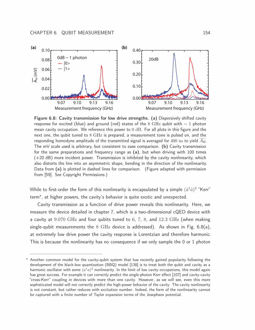
CHAPTER 6. QUBIT MEASUREMENT 154
(b)(a)
Figure 6.8: Cavity transmission for low drive strengths. (a) Dispersively shifted cavityresponse for excited (blue) and ground (red) states of the 8 GHz qubit with ∼ 1 photonmean cavity occupation. We reference this power to 0 dB. For all plots in this figure and thenext one, the qubit tuned to 8 GHz is prepared, a measurement tone is pulsed on, and theresponding homodyne amplitude of the transmitted signal is averaged for 400 ns to yield AH.The mV scale used is arbitrary, but consistent to ease comparison. (b) Cavity transmissionfor the same preparations and frequency range as (a), but when driving with 100 times(+20 dB) more incident power. Transmission is inhibited by the cavity nonlinearity, whichalso distorts the line into an asymmetric shape, bending in the direction of the nonlinearity.Data from (a) is plotted in dashed lines for comparison. (Figure adapted with permissionfrom [59]. See Copyright Permissions.)
While to first-order the form of this nonlinearity is encapsulated by a simple (a†a)2 “Kerr”term∗, at higher powers, the cavity’s behavior is quite exotic and unexpected.
Cavity transmission as a function of drive power reveals this nonlinearity. Here, wemeasure the device detailed in chapter 7, which is a two-dimensional cQED device witha cavity at 9.070 GHz and four qubits tuned to 6, 7, 8, and 12.3 GHz (when makingsingle-qubit measurements the 8 GHz device is addressed). As shown in Fig. 6.8(a),at extremely low drive power the cavity response is Lorentzian and therefore harmonic.This is because the nonlinearity has no consequence if we only sample the 0 or 1 photon
∗ Another common model for the cavity-qubit system that has recently gained popularity following thedevelopment of the black-box quantization (BBQ) model [138] is to treat both the qubit and cavity as aharmonic oscillator with some (a†a)2 nonlinearity. In the limit of low cavity occupations, this model againhas great success. For example it can correctly predict the single-photon Kerr effect [107] and cavity-cavity“cross-Kerr” coupling in devices with more than one cavity. However, as we will see, even this moresophisticated model will not correctly predict the high-power behavior of the cavity. The cavity nonlinearityis not constant, but rather reduces with excitation number. Indeed, the form of the nonlinearity cannotbe captured with a finite number of Taylor expansion terms of the Josephson potential.

CHAPTER 6. QUBIT MEASUREMENT 155
states. (The fact that two photons are not exactly twice the energy of one photon is notnoticed if we never populate the second photon). We also observe the dispersive shift,with transmission for the qubit prepared in the ground state in red and the excited state inblue. If we wanted to make a conventional measurement, we would drive at this power atabout 9.145 GHz (the red peak), inferring that the qubit was in the ground state if wegot a relatively high transmission and vice versa.
When we drive much harder, we start to see evidence of the cavity being non-harmonic.This is shown in Fig. 6.8(b), in which we have increased the drive power by a factor of100. We refer to this power as being +20 dB, where 0 dB is defined by the power thatproduces a one-photon mean cavity occupation. The cavity line shape is asymmetric, withthe slope on the low-frequency side being much steeper than that of the high-frequencyside. This is the canonical behavior of a Kerr-Duffing oscillator, where the negative cavityanharmonicity pushes the resonance down in frequency as the occupation increases. Thepeak transmitted homodyne amplitude would be a factor of 10 higher if the cavity werelinear but has only increased by a factor of 4. This is attributable to either pure cavitydephasing or a photon-blockading effect, where further excitation is inhibited when anadditional photon shifts the transition frequency of the cavity out of resonance with thedrive. Photon blockading would be correctly predicted by an (a†a)2 anharmonicity.
The photon-blockade or dephasing effect is even more dramatically illustrated inFig. 6.9(a). There we have increased the drive power by another factor of 100 but seean increase in homodyne voltage by less than a factor of two. (Note the presence of asquare root here, with the drive measured in power units but the transmission in voltageunits; we should expect only ten times more voltage in linear response.) The line shape nolonger resembles that of a conventional resonance: it is quite broad and rough and theexcited-state cavity transmission has shifted back toward the ground state, reducing thestate-dependent transmission difference. There is also a sharp dip at lower frequencies,possibly due to an interference between the multiple solutions of the now-bifurcated cavity[211].
For a long time, it was believed that this bifurcation was the end of the cavity-transmission-vs-power story. For the purposes of readout, increasing power would initiallyhelp, but not as much as it “should” if the cavity were linear because of photon blockadingeffects. Beyond a certain point, the cavity would be so distorted that the state-dependenttransmission difference would drop, and fidelity would suffer. Indeed, this would be trueif the cavity had a constant Kerr-type nonlinearity, which is well understood and even
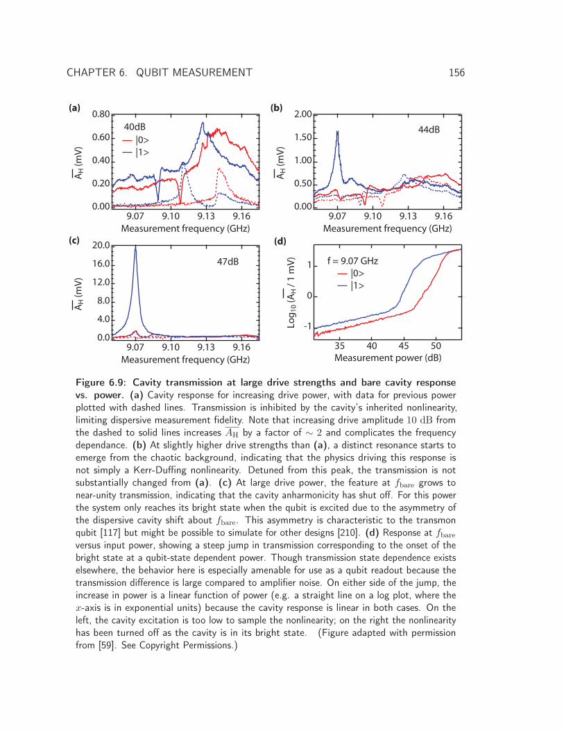
CHAPTER 6. QUBIT MEASUREMENT 156
(a) (b)
(c) (d)
Figure 6.9: Cavity transmission at large drive strengths and bare cavity responsevs. power. (a) Cavity response for increasing drive power, with data for previous powerplotted with dashed lines. Transmission is inhibited by the cavity’s inherited nonlinearity,limiting dispersive measurement fidelity. Note that increasing drive amplitude 10 dB fromthe dashed to solid lines increases AH by a factor of ∼ 2 and complicates the frequencydependance. (b) At slightly higher drive strengths than (a), a distinct resonance starts toemerge from the chaotic background, indicating that the physics driving this response isnot simply a Kerr-Duffing nonlinearity. Detuned from this peak, the transmission is notsubstantially changed from (a). (c) At large drive power, the feature at fbare grows tonear-unity transmission, indicating that the cavity anharmonicity has shut off. For this powerthe system only reaches its bright state when the qubit is excited due to the asymmetry ofthe dispersive cavity shift about fbare. This asymmetry is characteristic to the transmonqubit [117] but might be possible to simulate for other designs [210]. (d) Response at fbareversus input power, showing a steep jump in transmission corresponding to the onset of thebright state at a qubit-state dependent power. Though transmission state dependence existselsewhere, the behavior here is especially amenable for use as a qubit readout because thetransmission difference is large compared to amplifier noise. On either side of the jump, theincrease in power is a linear function of power (e.g. a straight line on a log plot, where thex-axis is in exponential units) because the cavity response is linear in both cases. On theleft, the cavity excitation is too low to sample the nonlinearity; on the right the nonlinearityhas been turned off as the cavity is in its bright state. (Figure adapted with permissionfrom [59]. See Copyright Permissions.)
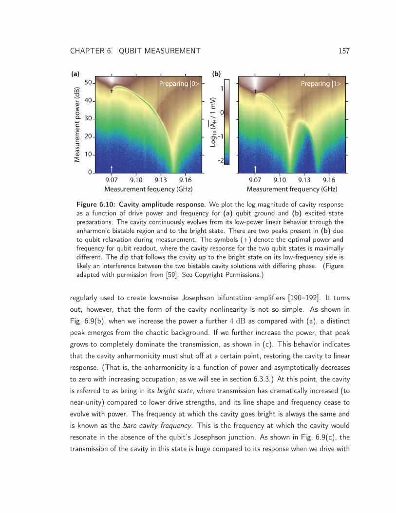
CHAPTER 6. QUBIT MEASUREMENT 157
(b)(a)
Figure 6.10: Cavity amplitude response. We plot the log magnitude of cavity responseas a function of drive power and frequency for (a) qubit ground and (b) excited statepreparations. The cavity continuously evolves from its low-power linear behavior through theanharmonic bistable region and to the bright state. There are two peaks present in (b) dueto qubit relaxation during measurement. The symbols (+) denote the optimal power andfrequency for qubit readout, where the cavity response for the two qubit states is maximallydifferent. The dip that follows the cavity up to the bright state on its low-frequency side islikely an interference between the two bistable cavity solutions with differing phase. (Figureadapted with permission from [59]. See Copyright Permissions.)
regularly used to create low-noise Josephson bifurcation amplifiers [190–192]. It turnsout, however, that the form of the cavity nonlinearity is not so simple. As shown inFig. 6.9(b), when we increase the power a further 4 dB as compared with (a), a distinctpeak emerges from the chaotic background. If we further increase the power, that peakgrows to completely dominate the transmission, as shown in (c). This behavior indicatesthat the cavity anharmonicity must shut off at a certain point, restoring the cavity to linearresponse. (That is, the anharmonicity is a function of power and asymptotically decreasesto zero with increasing occupation, as we will see in section 6.3.3.) At this point, the cavityis referred to as being in its bright state, where transmission has dramatically increased (tonear-unity) compared to lower drive strengths, and its line shape and frequency cease toevolve with power. The frequency at which the cavity goes bright is always the same andis known as the bare cavity frequency. This is the frequency at which the cavity wouldresonate in the absence of the qubit’s Josephson junction. As shown in Fig. 6.9(c), thetransmission of the cavity in this state is huge compared to its response when we drive with
CHAPTER 6. QUBIT MEASUREMENT 158
only a few dBs lower power. Transmission for the two qubit preparations is summarized inFig. 6.10.
The strongly-driven Jaynes-Cummings Hamiltonian has been previously studied for thecase of the cavity and qubit in resonance [210]. There, at drive strengths so high thatthey would be inaccessible with essentially any other system, higher-order photon numberresonances with characteristic
√n spacing appear, in excellent agreement with theory. The
dispersive limit was not studied for the reasons described in the previous paragraph, butthe story is similar. We can reach a regime of the Hamiltonian where the drive strength(or, excitation level) is so high that qualitatively new physics emerges [59, 210, 212]. Incontrast to the resonant case and to our great fortune and surprise, this new physics haspractical applications for the purposes of qubit measurement.
6.3.2 Single and multi-qubit measurement
The ability to use this phenomenon to read out the qubit was demonstrated in Fig. 6.9(c).There, we have driven the cavity to the bright state for the qubit in the excited state,but not for the ground state. The transmission difference at the bare cavity frequencyis therefore huge. We get a small signal driving at 9.070 GHz with 47 dB if the qubitis in its ground state but a very large one if it is excited. Qualitatively, this is the samemechanism we use for the dispersive readout. The primary difference here is that we aredealing with much larger signals. In the case of the dispersive readout, we have a meancavity occupation of approximately ten photons; in this device, there are thousands oftimes more. Thus, our measurement fidelity is not dominated by the signal-to-noise ratio,nor set by things like amplifier noise. (Let us hasten to point out that a very large SNRfor distinguishing the bright state from the dim state does not imply unity measurementfidelity; the mapping of the qubit state onto the semi-classical cavity pointer state can stillbe imperfect.)
The emergence of the high-power peak, we postulated, results from the fact that at acertain occupation the cavity anharmonicity reduces to zero (or at least to less than thecavity linewidth). This explanation made no mention of the qubit state, however, so whydo we see a state dependence of the critical power? It originates from the same underlyingphysics as the conventional low-power readout: the qubit-state selective dispersive cavityshift. In our prescription for measurement using this effect, we drive at the bare cavityfrequency with a certain power. This means that we are initially driving far off-resonant
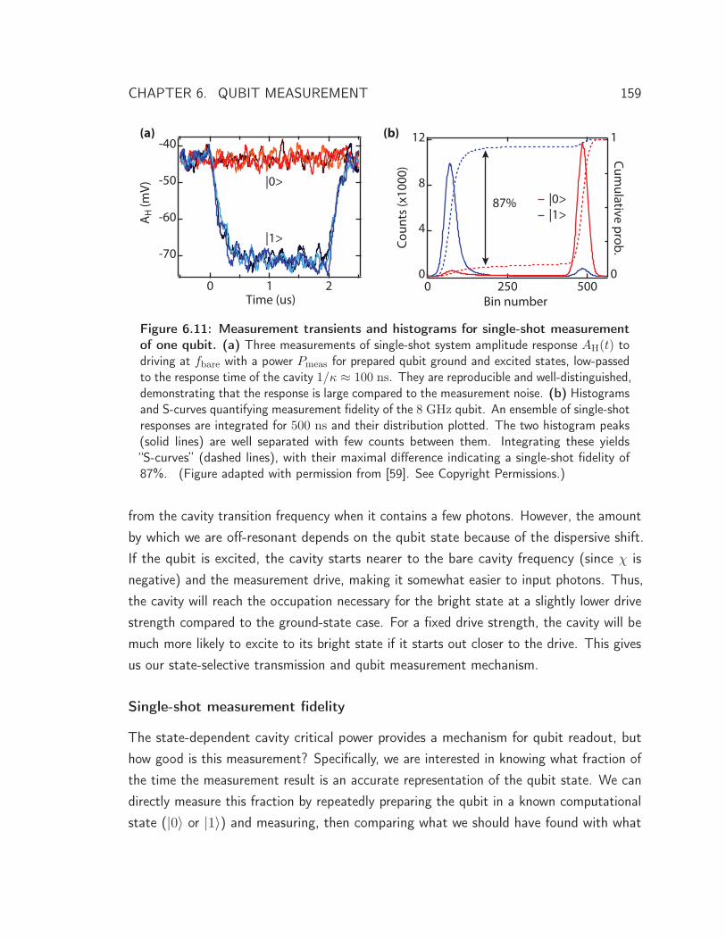
CHAPTER 6. QUBIT MEASUREMENT 159
(a) (b)
87%
Figure 6.11: Measurement transients and histograms for single-shot measurementof one qubit. (a) Three measurements of single-shot system amplitude response AH(t) todriving at fbare with a power Pmeas for prepared qubit ground and excited states, low-passedto the response time of the cavity 1/κ ≈ 100 ns. They are reproducible and well-distinguished,demonstrating that the response is large compared to the measurement noise. (b) Histogramsand S-curves quantifying measurement fidelity of the 8 GHz qubit. An ensemble of single-shotresponses are integrated for 500 ns and their distribution plotted. The two histogram peaks(solid lines) are well separated with few counts between them. Integrating these yields“S-curves” (dashed lines), with their maximal difference indicating a single-shot fidelity of87%. (Figure adapted with permission from [59]. See Copyright Permissions.)
from the cavity transition frequency when it contains a few photons. However, the amountby which we are off-resonant depends on the qubit state because of the dispersive shift.If the qubit is excited, the cavity starts nearer to the bare cavity frequency (since χ isnegative) and the measurement drive, making it somewhat easier to input photons. Thus,the cavity will reach the occupation necessary for the bright state at a slightly lower drivestrength compared to the ground-state case. For a fixed drive strength, the cavity will bemuch more likely to excite to its bright state if it starts out closer to the drive. This givesus our state-selective transmission and qubit measurement mechanism.
Single-shot measurement fidelity
The state-dependent cavity critical power provides a mechanism for qubit readout, buthow good is this measurement? Specifically, we are interested in knowing what fraction ofthe time the measurement result is an accurate representation of the qubit state. We candirectly measure this fraction by repeatedly preparing the qubit in a known computationalstate (|0〉 or |1〉) and measuring, then comparing what we should have found with what
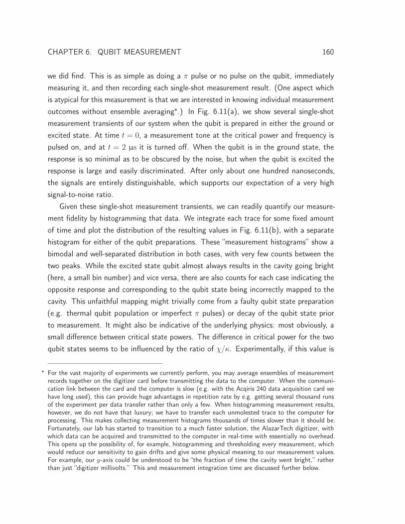
CHAPTER 6. QUBIT MEASUREMENT 160
we did find. This is as simple as doing a π pulse or no pulse on the qubit, immediatelymeasuring it, and then recording each single-shot measurement result. (One aspect whichis atypical for this measurement is that we are interested in knowing individual measurementoutcomes without ensemble averaging∗.) In Fig. 6.11(a), we show several single-shotmeasurement transients of our system when the qubit is prepared in either the ground orexcited state. At time t = 0, a measurement tone at the critical power and frequency ispulsed on, and at t = 2 μs it is turned off. When the qubit is in the ground state, theresponse is so minimal as to be obscured by the noise, but when the qubit is excited theresponse is large and easily discriminated. After only about one hundred nanoseconds,the signals are entirely distinguishable, which supports our expectation of a very highsignal-to-noise ratio.
Given these single-shot measurement transients, we can readily quantify our measure-ment fidelity by histogramming that data. We integrate each trace for some fixed amountof time and plot the distribution of the resulting values in Fig. 6.11(b), with a separatehistogram for either of the qubit preparations. These “measurement histograms” show abimodal and well-separated distribution in both cases, with very few counts between thetwo peaks. While the excited state qubit almost always results in the cavity going bright(here, a small bin number) and vice versa, there are also counts for each case indicating theopposite response and corresponding to the qubit state being incorrectly mapped to thecavity. This unfaithful mapping might trivially come from a faulty qubit state preparation(e.g. thermal qubit population or imperfect π pulses) or decay of the qubit state priorto measurement. It might also be indicative of the underlying physics: most obviously, asmall difference between critical state powers. The difference in critical power for the twoqubit states seems to be influenced by the ratio of χ/κ. Experimentally, if this value is
∗ For the vast majority of experiments we currently perform, you may average ensembles of measurementrecords together on the digitizer card before transmitting the data to the computer. When the communi-cation link between the card and the computer is slow (e.g. with the Acqiris 240 data acquisition card wehave long used), this can provide huge advantages in repetition rate by e.g. getting several thousand runsof the experiment per data transfer rather than only a few. When histogramming measurement results,however, we do not have that luxury; we have to transfer each unmolested trace to the computer forprocessing. This makes collecting measurement histograms thousands of times slower than it should be.Fortunately, our lab has started to transition to a much faster solution, the AlazarTech digitizer, withwhich data can be acquired and transmitted to the computer in real-time with essentially no overhead.This opens up the possibility of, for example, histogramming and thresholding every measurement, whichwould reduce our sensitivity to gain drifts and give some physical meaning to our measurement values.For example, our y-axis could be understood to be “the fraction of time the cavity went bright,” ratherthan just “digitizer millivolts.” This and measurement integration time are discussed further below.
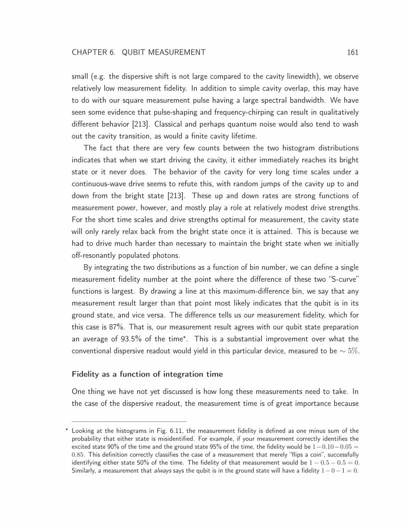
CHAPTER 6. QUBIT MEASUREMENT 161
small (e.g. the dispersive shift is not large compared to the cavity linewidth), we observerelatively low measurement fidelity. In addition to simple cavity overlap, this may haveto do with our square measurement pulse having a large spectral bandwidth. We haveseen some evidence that pulse-shaping and frequency-chirping can result in qualitativelydifferent behavior [213]. Classical and perhaps quantum noise would also tend to washout the cavity transition, as would a finite cavity lifetime.
The fact that there are very few counts between the two histogram distributionsindicates that when we start driving the cavity, it either immediately reaches its brightstate or it never does. The behavior of the cavity for very long time scales under acontinuous-wave drive seems to refute this, with random jumps of the cavity up to anddown from the bright state [213]. These up and down rates are strong functions ofmeasurement power, however, and mostly play a role at relatively modest drive strengths.For the short time scales and drive strengths optimal for measurement, the cavity statewill only rarely relax back from the bright state once it is attained. This is because wehad to drive much harder than necessary to maintain the bright state when we initiallyoff-resonantly populated photons.
By integrating the two distributions as a function of bin number, we can define a singlemeasurement fidelity number at the point where the difference of these two “S-curve”functions is largest. By drawing a line at this maximum-difference bin, we say that anymeasurement result larger than that point most likely indicates that the qubit is in itsground state, and vice versa. The difference tells us our measurement fidelity, which forthis case is 87%. That is, our measurement result agrees with our qubit state preparationan average of 93.5% of the time∗. This is a substantial improvement over what theconventional dispersive readout would yield in this particular device, measured to be ∼ 5%.
Fidelity as a function of integration time
One thing we have not yet discussed is how long these measurements need to take. Inthe case of the dispersive readout, the measurement time is of great importance because
∗ Looking at the histograms in Fig. 6.11, the measurement fidelity is defined as one minus sum of theprobability that either state is misidentified. For example, if your measurement correctly identifies theexcited state 90% of the time and the ground state 95% of the time, the fidelity would be 1−0.10−0.05 =0.85. This definition correctly classifies the case of a measurement that merely “flips a coin”, successfullyidentifying either state 50% of the time. The fidelity of that measurement would be 1− 0.5− 0.5 = 0.Similarly, a measurement that always says the qubit is in the ground state will have a fidelity 1−0−1 = 0.
CHAPTER 6. QUBIT MEASUREMENT 162
(a) (b) (c)
(d) (e) (f)
(g)
Figure 6.12: Measurement histograms and fidelity versus integration time. (a-f)Histograms of single-qubit measurements as a function of integration time. Here, thesame measurement transient dataset are processed and histogrammed, but with a variableintegration as specified in each window. At short times, the histograms are essentiallyoverlapping, but for longer measurements they evolve apart and entirely separate. (g)Measurement fidelity as a function of integration time. Integrating VH(t) for 120 ns yields80% fidelity, while 240 ns yields 87%. After that point, the fidelity has saturated andincreasing the SNR does not improve the result. We are limited by the cavity pointer stateincorrectly mapping the qubit state, rather than an inability to distinguish the pointer state.Additional integration does increase the histogram separation, however, which may be usefulif we are thresholding the data to convert a voltage to an estimated qubit state. (Figureadapted with permission from [59]. See Copyright Permissions.)
CHAPTER 6. QUBIT MEASUREMENT 163
the qubit can decay, so further integration after this occurs lowers the fidelity. In the caseof the bright state readout, however, once the cavity has decided to go bright or not, ittends to stay that way – that is, this is a latching readout. As a result, we have the luxuryof integrating as long as we like to get whatever SNR we desire. In Fig. 6.12, we showthe resulting measurement fidelity for varying measurement integration times. For thisdevice, the measurement fidelity smoothly increases from 0 to 80% in the first 100 ns,and levels off at its final value of 87% by 175 ns. This time is likely due to either thespeed with which the system excites to the bright state, or simply how long it takes forthe measurement chain noise to be drowned out by our growing signal.
Integrating for more than 240 ns does not increase fidelity in this device because weare limited by unfaithful qubit state mapping; it does, however, increase the signal-to-noiseratio. We can see this increase by plotting the measurement histograms as a function ofintegration time. After only 20 ns the distributions are virtually identical, but they splitinto our bimodal distribution as we integrate longer. By 120 ns, the fidelity has almostreached its final value, but the distributions remain close to one another. Integrating for300 ns or 500 ns does not substantially change the measurement fidelity but does increasethe open space between the peaks. This has one practical benefit. If we were to use afast digitizer to “threshold” the data at our optimal fidelity point, turning distributions ofmeasurements into ones and zeros, having extra open space around the threshold valuemakes that process more robust. Drifts in the gain or offsets of the measurement chainwill not tend to change the thresholded measurement outcome for long integration times,while they might for smaller SNRs of the same nominal fidelity.
Multi-qubit measurement
We can extend this readout scheme to simultaneously measure multiple qubits. The physicsof multi-qubit readout is similar to the single-qubit case, but generalized for multiple basisstates. Each qubit has its own dispersive shift χi, and since for e.g. three qubits there areeight separate basis states, there will be eight zero-power cavity frequencies. For example,the state |011〉, where the second and third qubits are excited, will shift the cavity by2χ2 + 2χ3. Since each basis state induces a different net dispersive cavity shift, there willbe a hierarchy of drive strengths necessary to drive each cavity to the bright state. Readoutis done by choosing a measurement drive power above the onset power for all except thestate or states one is trying to distinguish. That way, the cavity should go bright for the

CHAPTER 6. QUBIT MEASUREMENT 164
Figure 6.13: Pulsed cavity response AH for |111〉 state. The eight (23) regis-ter states of three qubits induce a different dispersive cavity shift, each discernible atlow power due to decay of the |111〉 state during measurement. These frequencieswere independently measured to be (f|000〉, f|100〉, f|010〉, f|001〉, f|110〉, f|101〉, f|011〉, f|111〉) =(9.145, 9.139, 9.131, 9.112, 9.124, 9.105, 9.097, 9.090) GHz, with fbare = 9.070 GHz. Themost prominent secondary cavity position corresponds to the third qubit (at 8 GHz) relaxingduring measurement, consistent with its Purcell-limited [139] T1 being the shortest of thethree, with TQ1
1 = 1.2 μs, TQ21 = 1.0 μs, and TQ3
1 = 0.6 μs. The system excites to itsbright state at lower power here than seen in Fig. 6.10 because of the smaller initial cavitydetuning from fbare. The color scale is identical to that in Fig. 6.10. (Figure adapted withpermission from [59]. See Copyright Permissions.)
states with critical powers below the selected drive power, and stay dim otherwise, againgiving us a single classical bit of information. This scheme is especially convenient forperforming qubit state tomography [214], which requires inferring multi-qubit correlations[121, 215, 216]. As discussed in section 7.3, the effective measurement operator for thisscheme is
∣∣0⊗N⟩⟨0⊗N
∣∣ and contains all Z correlations. As we will see, this fact has beenexploited to efficiently detect tripartite entanglement [55].
The device that we first demonstrated this effect with had a total of four qubits.Three were tuned to 6, 7, and 8 GHz, with the fourth at high frequency and unused(section 7.1). In Fig. 6.13, we show transmission as a function of frequency and powerwhen the |111〉 state (where all three qubits are in their first excited state) is prepared. Atlow drive strengths, eight separate cavity peaks are visible because |111〉 has the possibilityof decaying into each of the other seven basis states. The cavity reaches its bright state at
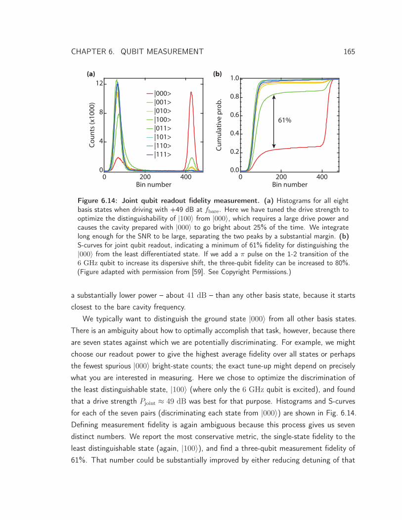
CHAPTER 6. QUBIT MEASUREMENT 165
61%
(a) (b)
Figure 6.14: Joint qubit readout fidelity measurement. (a) Histograms for all eightbasis states when driving with +49 dB at fbare. Here we have tuned the drive strength tooptimize the distinguishability of |100〉 from |000〉, which requires a large drive power andcauses the cavity prepared with |000〉 to go bright about 25% of the time. We integratelong enough for the SNR to be large, separating the two peaks by a substantial margin. (b)S-curves for joint qubit readout, indicating a minimum of 61% fidelity for distinguishing the|000〉 from the least differentiated state. If we add a π pulse on the 1-2 transition of the6 GHz qubit to increase its dispersive shift, the three-qubit fidelity can be increased to 80%.(Figure adapted with permission from [59]. See Copyright Permissions.)
a substantially lower power – about 41 dB – than any other basis state, because it startsclosest to the bare cavity frequency.
We typically want to distinguish the ground state |000〉 from all other basis states.There is an ambiguity about how to optimally accomplish that task, however, because thereare seven states against which we are potentially discriminating. For example, we mightchoose our readout power to give the highest average fidelity over all states or perhapsthe fewest spurious |000〉 bright-state counts; the exact tune-up might depend on preciselywhat you are interested in measuring. Here we chose to optimize the discrimination ofthe least distinguishable state, |100〉 (where only the 6 GHz qubit is excited), and foundthat a drive strength Pjoint ≈ 49 dB was best for that purpose. Histograms and S-curvesfor each of the seven pairs (discriminating each state from |000〉) are shown in Fig. 6.14.Defining measurement fidelity is again ambiguous because this process gives us sevendistinct numbers. We report the most conservative metric, the single-state fidelity to theleast distinguishable state (again, |100〉), and find a three-qubit measurement fidelity of61%. That number could be substantially improved by either reducing detuning of that

CHAPTER 6. QUBIT MEASUREMENT 166
qubit or by performing a π pulse on the 1-2 transition of that qubit prior to measurementto increase its effective dispersive shift. When that pulse is included in the measurementprocess, the joint fidelity here is increased to about 80%. Note that optimizing againstthis state necessarily reduces the fidelity to the others. That optimization leads us to driverather strongly, giving a ∼ 25% chance of the cavity exciting for the ground state; allother fidelities are reduced by this factor.
6.3.3 Theory of the Jaynes-Cummings nonlinearity
Now that we have presented the experimental observations of the high-power cavity responseand its application to measurement, let us return to the discussion of the underlying physics.This section will largely summarize the result of [210], which qualitatively predicts the mainfeatures of the Jaynes-Cummings readout from first principles. Bishop et al. consider theJaynes-Cummings Hamiltonian of a two-level qubit coupled to a cavity under the influenceof a drive:
H = ωra†a+
ωq
2σz + g
(aσ+ + a†σ−
)+
ξ(t)√2
(a+ a†
)(6.4)
where ωr/2π is the cavity frequency, ωq/2π the qubit frequency, g the coupling strength,and ξ(t) = ξcos(ωdt) is the drive of amplitude ξ and frequency ωd. They then makethe “bad-cavity” and strong-dispersive approximations, where the cavity lifetime is shortcompared to the qubit decay and dephasing rates (κ > γ, γφ) and the qubit-cavity dispersiveshift χ is greater than κ, respectively. Dropping small terms, this yields the effectiveHamiltonian
˜H = ωra
†a+ (ωr − Δ)σz
2+
ξ√2
(a+ a†
)cos(ωdt). (6.5)
This equation could be (and has been) integrated numerically with a quantum masterequation [210]. That is challenging here because there will be a large number of photons forrelevant drive strengths and so the Hilbert space is huge. Instead, if the cavity anharmonicityis smaller than its linewidth (e.g. the N − 1 ↔ N and N ↔ N + 1 transition peaksoverlap, or N � g4/κδ3), a semiclassical model will be a good approximation. This isespecially attractive given that the typical approach of perturbatively expanding Eq. 6.4 inpowers of N/Ncrit will not converge when N > Ncrit. There, the critical photon numberNcrit = δ2/4g2 and δ is the cavity-qubit detuning. For the parameters of this device,Ncrit ∼ 6, so this is a very stringent limit.
Bishop rewrites Eq. 6.4 using canonical variables X =√
1/2(a† + a
)and P =
CHAPTER 6. QUBIT MEASUREMENT 167
i√
1/2(a† − a
)to give
H =ωr
2
(X2 + P 2 + σz
)+ ξXcos(ωdt) − σz
2
√2g2 (X2 + P 2 + σz) + δ2. (6.6)
Treating X and P as numbers (and not operators) in the semiclassical approximation, andincorporating cavity decay with an additional damping term, we solve for the steady stateamplitude A =
√X2 + P 2 as
A2 =ω2rξ
2
{ω2d − [ωr − χ(A)]2}2 + κ2ω2
d
(6.7)
with the cavity dispersive shift χ(A) depending on cavity amplitude as
χ(A) = σzg2√
2g2 (A2 + σz) + δ2. (6.8)
This equation satisfies the normal approximation for the dispersive shift for a Cooper-pairbox (e.g. two-level qubit) with χ(0) ≈ ±g2/δ. Crucially, under strong driving it alsosaturates with limA→∞χ(A) = 0.
With this result, we can start predicting the behavior of the cavity as a function ofdrive strength. We expect the anharmonicity of the cavity (e.g. the difference in χ for Nand N + 1 excitations) to be maximal at low power and continuously diminish as the drivestrength is increased. At the zero-power limit, we will see a linear response because weare only populating the 0 and 1 photon states and never sample the nonlinearity. As weincrease the drive strength, however, the anharmonicity will turn on and distort our lineshape, consistent with Fig. 6.8.
At slightly higher drive strengths, based on our experience with Kerr nonlinearities,we expect the frequency response to bifurcate into two solutions. The phases of the twosolutions, one “dim” and one “bright,” will be almost opposite since they are effectively onalternate sides of the resonance. This bifurcation is observed in the numerical simulationsof Eq. 6.7 done by Bishop, et al. As the drive strength is turned up, rather than thebistable region growing forever with power as with a Kerr oscillator, the region shrinks andeventually vanishes, emphasizing that this cavity’s nonlinearity is not constant. This pointcorresponds exactly with the bare cavity frequency and critical power. As a consequence,when driving at the bare cavity frequency, the system is never bistable (at least in thismodel’s approximation). Moreover, this bifurcation is responsible for the appearance of thedip in Fig. 6.10 that traces up to the high-power peak. We expect destructive interference
CHAPTER 6. QUBIT MEASUREMENT 168
at the point where the populations of the two solutions are similar, weighted by theswitching rates [211]. This occurs where our heterodyne detection coherently averagesover the ensemble of experiments.
Finally, for increasing drive strength at the bare cavity frequency, the cavity populationincreases and anharmonicity shrinks. At some critical power, where χ(N) � κ, we drivehard enough for the cavity to shift into resonance with the drive. At this point, itspopulation (and therefore transmission) rapidly grow while its anharmonicity shrinks – thusreaching the bright state. Note that this point (where we say N = Nbare) necessarilyhappens at a much larger drive strength than Ncrit, so a perturbative expansion wouldfail to reveal this behavior. It is unsurprising that this phenomenon was not theoreticallypredicted prior to its experimental discovery. By looking at the numerical solution shownin the Bishop paper, we also see that the semiclassical model predicts the qualitativeresponse as a function of drive power at the bare cavity frequency shown in Fig. 6.10(a).The success of this model at predicting essentially all of the behavior of the cavity isquite remarkable considering that it is a vast simplification relative to the actual systemHamiltonian.
One detail worth mentioning is that the model presented above does not predict thatthis would work as a readout mechanism. The model assumes a two-level atom, implyingthat the dispersive cavity shift will be symmetric about the bare cavity frequency. Withoutan asymmetry, the critical power for both cases would be essentially the same (brokenonly by qubit relaxation), eliminating our state-dependent transmission. In order to havecontrast, this symmetry must be broken. For our system, this is accomplished by the factthat our qubits are actually weakly anharmonic transmon oscillators with higher excitedstates. The repulsion of the states |e, n+ 1〉 and |f, n〉 (where e is the first excited qubitstate and f the second) of the undressed Hamiltonian would, for example, be sufficientasymmetry. Alternatively, if more than one two-level system were available, the extra shiftfrom that qubit would give contrast to any single qubit, though not both jointly (since e.g.the |00〉 and |11〉 states would have the same shift).
6.3.4 JCR summary
Using the Jaynes-Cummings cavity nonlinearity to measure qubits has the significantadvantage of delivering high fidelity without requiring any additional experimental hardwareor change of sample design. Essentially, we are using the qubit as its own amplifier. Its
CHAPTER 6. QUBIT MEASUREMENT 169
fidelity is virtually independent of cavity Q as long as χ > κ. We have observed excellentmeasurement fidelities with cavity Q’s ranging from a few hundred to several million. (Notethat this would not be true of a dispersive measurement, since its information collectionrate is proportional to κ.) The effect is seen in every cavity coupled to a transmon qubit.As discussed in section 5.1.1, it can even serve as a quick verification that qubits arepresent. We can measure the cavity at high power and then see if it either disappearsabruptly or shifts in frequency as the power is lowered to detect the presence of a qubit,and estimate how strongly it is coupled or how far it is detuned using the difference infrequency between the high- and low-power cavity frequencies.
There are some practical aspects which are not fully understood. Occasionally, thecritical power seems to have a “switchy” behavior, seeming to randomly jump between twoor more values. The source of this tendency is unknown, but it is seemingly mitigated byeither using slightly lower measurement power or by waiting for the system to “calm down”(it seems to happen more frequently shortly after the device is cooled). When a qubitis positively detuned from the cavity, the readout is typically not as reliable because thecavity nonlinearity will have to change its sign. The gain curve analogous to Fig. 6.9(d)can also exhibit a double-step behavior where the cavity seems to go bright in two distincttransitions when the qubit is far detuned or weakly coupled. There, the understandingof an asymptotically decreasing anharmonicity is no longer true. Though the physics aresignificantly more complex, it still seems to work as a reliable measurement mechanism.
Experimental repetition rates and qubit T1s can also be affected by the high-powerreadout. We did not initially notice any difference between the dispersive and high-powerreadout when using a relatively low-Q cavity. However, the 3D cQED architecture featuresphoton lifetimes so long that the difference between waiting for a few dozen and a fewthousand measurement photons to decay can be meaningful. We have seen that if therepetition rate is not slow enough, the qubit T1 and T2 can be adversely affected. Therepetition rate required can also sometimes be much longer than one would expect fromeither the qubit or cavity decay time. Since the 3D architecture generally operates in amuch larger value of χ/κ, the drive power needed to off-resonantly drive the cavity to itsbright state can be extremely large and populate a huge number of photons if the cavityis allowed to come into equilibrium. We therefore speculate that we might be drivingthe qubit junction to its normal state, and so are required to wait for quasiparticles torecombine. One way of mitigating this effect would be to chirp the frequency of the drivetone from the low-power cavity down to the bare cavity frequency while its amplitude is
CHAPTER 6. QUBIT MEASUREMENT 170
increased [213]. This would lower the effective critical power as well as the total energyneeded for measurement.
This readout mechanism is only appropriate for the end of an experiment because it isnot QND to the qubit state. In order to drive the cavity to its bright state, it is necessaryto dump so much power into the cavity that the qubit state seems to be scrambled andlikely left in a highly excited state. This is likely due to some combination of dresseddephasing, qubit dressing [212], or direct qubit transitions. For experiments in whichmeasurements must be QND, the Jaynes-Cummings readout is not an option.
6.4 Conclusion
Qubit measurement in cQED is accomplished by taking advantage of the dispersive shiftof the cavity frequency. Applying a displacement to the cavity therefore entangles thecavity together with the qubit state. This displacement leaks out and is absorbed by ouramplifier chain, projecting the qubit superposition along the z-axis. If we have a highenough signal to noise ratio, we can detect this transmitted light to infer the state of thequbit. With a conventional amplifier chain, this transmission is combined with a largeamount of amplifier noise which obscures our ability to distinguish the signal. The signalpower is also limited by the cavity lifetime, which cannot be made too short because thePurcell effect will reduce qubit lifetime. One solution to this is to use a so-called Purcellfilter, which breaks the cavity-qubit lifetime relationship. This apparatus has the ancillarybenefit of increasing the dynamic range in qubit lifetime, which can be used for efficientqubit reset.
For conventional dispersive readout, the equilibrium number of cavity photons is limitedby cavity anharmonicity. Beyond a certain drive strength, the cavity’s inherited nonlinearitywill corrupt its response, reducing measurement fidelity as power is increased. The natureof this nonlinearity is quite special since it turns off at extremely high drive strengths, givingthe cavity a linear response at its bare cavity frequency. Because the drive strength requiredto drive the cavity to this high-transmission state depends on the initial cavity detuningand thus on the qubit state, the effect can be used to readout the qubit state. Thismechanism, known as the Jaynes-Cummings or simply high-power readout∗, is extremely
CHAPTER 6. QUBIT MEASUREMENT 171
robust to device parameters. Moreover, because the cavity is so highly excited and emits alarge signal, its fidelity is not limited by amplifier chain noise and can be quite high.
The question of which readout mechanism is the “best” arises. The choice often comesdown to experimental requirements. If a QND measurement is not required and fidelitiesof ∼ 90% are acceptable, the high-power JC readout is extremely attractive. It does notrequire any special hardware and will deliver relatively high fidelity across a wide range inqubit and cavity parameters. Additionally, it always operates at the same cavity frequencyindependent of qubit detuning, and thus is easy to tune up. Its main disadvantage is thatit is not QND to the qubit state. If you wish to make a qubit measurement and thenmanipulate the system as a result of that measurement (a function that will be extremelycommon in a “real” error-corrected quantum computer), the JCR will not work since thelarge number of cavity photons seem to scramble the qubit state. There are other potentialdownsides to this scheme as well: the large amount of energy deposited in the cavity issuspected to heat up the system and create quasiparticles that may adversely affect qubitcoherence. The system also seems to require a long time to relax back to its ground state,reducing the experimental repetition rate that can be used.
The dispersive readout mechanism solves many of these issues, but introduces someof its own. Since an extremely small amount of power is used, it can be QND to thequbit state and allow for repeated feed-forward measurements. This small amount ofenergy decays quickly, which potentially speeds up experimental repetitions. However, thesmall signal power is difficult to distinguish from conventional amplifier noise, requiringsophistications like the Purcell filter or ultra-low noise amplifiers to attain high measurementfidelity. Fidelity is also a strong function of system parameters (cavity Q, qubit couplingand detuning, etc), which complicates sample design, especially for experiments that arenot strictly about qubit measurement. Nevertheless, it is clear that when implementedcorrectly, the dispersive mechanism can provide a well-understood, high-fidelity, and QNDqubit measurement. If a cQED quantum computer is ever built, it will certainly use someform of the dispersive readout mechanism.
∗ Calling it the “Reedout” has also been known to happen, as a play on words with my last name.


CHAPTER 7
Tripartite Entanglement on Demand
We now turn our attention to generating and measuring entanglement in the cQEDarchitecture. This chapter serves two primary purposes. First: to report our result
of generating an entangled state of three qubits known as a Greenberger-Horne-Zeilingeror GHZ state. As we saw in section 2.3.4, this state is of great interest because it is aprerequisite for demonstrating the simplest form of quantum error correction. In showinghow we generate a GHZ state, we will explain how to engineer and tune up entanglinggates and introduce the distinction between adiabatic and sudden quantum trajectories.The second purpose of this chapter is to introduce the idea of measuring quantum systemswith tomography, which is useful for verifying the states and processes we claim to control.Virtually everything discussed here will be revisited when we demonstrate quantum errorcorrection in chapter 8. Many ideas presented here are also not specific to cQED, and canbe applied to any quantum computing platform.
In the first section, we introduce the four-qubit device used to generate GHZ statesand explain how the device is operated and calibrated. Each qubit has its own flux bias linewhich is used to tune qubit frequencies in-situ. We use them in two different limits: DCand fast-flux, respectively used to set the default frequency of each qubit and to tune theirfrequency rapidly to generate entanglement. The flux lines must be calibrated for bothtasks. In the case of DC flux, there is substantial cross-coupling between each flux line
173
CHAPTER 7. TRIPARTITE ENTANGLEMENT ON DEMAND 174
and the neighboring qubits which can be measured and inverted to make virtual controlknobs that address only one qubit. For fast-flux, we need to apply a deconvolution kernelto compensate for ringing and finite bandwidth. Using these linearized control knobs, weshow pulsed spectroscopy of Q1 moving up in frequency through avoided crossings withQ2, Q3, and the cavity.
Taking the qubit-qubit avoided crossings as an impetus, we then discuss how to engineerthe controlled-phase gates used to generate entanglement between qubits. We start byproposing a hypothetical “J-swap” gate that directly accesses the interaction zone betweentwo qubits. While this process would work to generate entanglement [217], we find that itfails to be the desired gate in the case of |11〉 due to an interaction that was not revealedin single-tone pulsed spectroscopy. Using two-tone spectroscopy technique, we measurethe additional avoided crossing between the higher-excited |11〉 and |02〉 states, thusaccounting for the failure of the J-swap. We show how this crossing, rather than being anobstacle, can be used to produce two different kinds of controlled-phase entangling gatesby moving into the crossing either adiabatically or suddenly.
Having established our ability to entangle qubits, we then describe how we measureand prove that the intended state was produced. We reconstruct the density matrix ofan ensemble of our states by repeatedly measuring certain correlations, a process knownas state tomography. The conventional method of obtaining these correlations involvesmeasuring each of the three qubits individually and calculating the correlations withclassical post-processing. However, because we lack the ability to measure the qubitsindividually, we use an alternate method. Our measurement operator is (approximately)M =
∣∣0⊗N⟩⟨0⊗N
∣∣, which can be expressed as a sum of all combinations of Z and I Paulioperators. By rotating the qubits immediately prior to measurement, we can effectivelymodify this measurement operator to contain all the Pauli correlations we seek. Applyinga full set of rotations, we produce sufficient linearly-independent measurement operatorsto infer every Pauli correlation and fully specify the experimental density matrix. Wedemonstrate this capability with several simple test states.
We can extend this idea to perform tomography on a quantum process. This techniquetells us the full action of any quantum process by measuring state tomograms of a sufficientnumber of states to span the full Hilbert space. These data can be converted to a χ-matrixwhich maps input density matrices to output density matrices. We demonstrate thistechnique by measuring the process matrix of a two-qubit controlled-phase gate. Theconventional χ-matrix representation is difficult to interpret beyond its fidelity and is
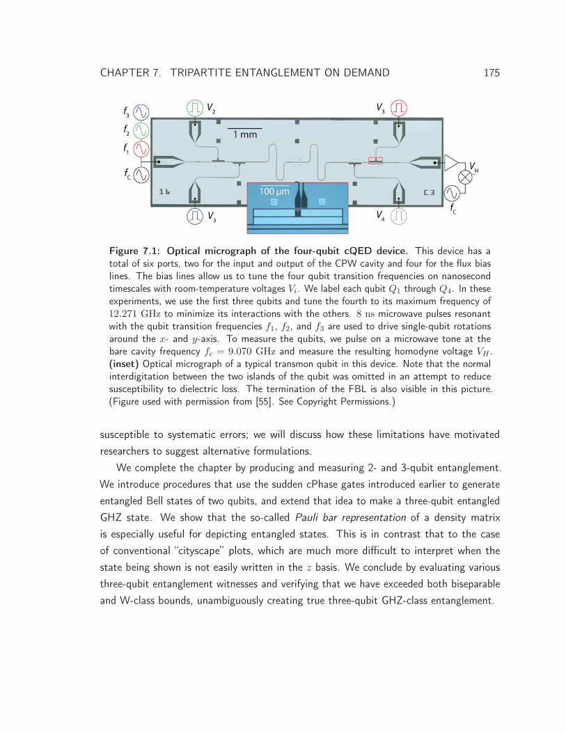
CHAPTER 7. TRIPARTITE ENTANGLEMENT ON DEMAND 175
Figure 7.1: Optical micrograph of the four-qubit cQED device. This device has atotal of six ports, two for the input and output of the CPW cavity and four for the flux biaslines. The bias lines allow us to tune the four qubit transition frequencies on nanosecondtimescales with room-temperature voltages Vi. We label each qubit Q1 through Q4. In theseexperiments, we use the first three qubits and tune the fourth to its maximum frequency of12.271 GHz to minimize its interactions with the others. 8 ns microwave pulses resonantwith the qubit transition frequencies f1, f2, and f3 are used to drive single-qubit rotationsaround the x- and y-axis. To measure the qubits, we pulse on a microwave tone at thebare cavity frequency fc = 9.070 GHz and measure the resulting homodyne voltage VH .(inset) Optical micrograph of a typical transmon qubit in this device. Note that the normalinterdigitation between the two islands of the qubit was omitted in an attempt to reducesusceptibility to dielectric loss. The termination of the FBL is also visible in this picture.(Figure used with permission from [55]. See Copyright Permissions.)
susceptible to systematic errors; we will discuss how these limitations have motivatedresearchers to suggest alternative formulations.
We complete the chapter by producing and measuring 2- and 3-qubit entanglement.We introduce procedures that use the sudden cPhase gates introduced earlier to generateentangled Bell states of two qubits, and extend that idea to make a three-qubit entangledGHZ state. We show that the so-called Pauli bar representation of a density matrixis especially useful for depicting entangled states. This is in contrast that to the caseof conventional “cityscape” plots, which are much more difficult to interpret when thestate being shown is not easily written in the z basis. We conclude by evaluating variousthree-qubit entanglement witnesses and verifying that we have exceeded both biseparableand W-class bounds, unambiguously creating true three-qubit GHZ-class entanglement.
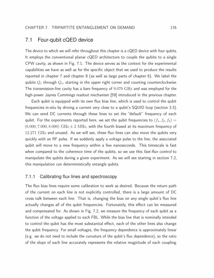
CHAPTER 7. TRIPARTITE ENTANGLEMENT ON DEMAND 176
7.1 Four-qubit cQED device
The device to which we will refer throughout this chapter is a cQED device with four qubits.It employs the conventional planar cQED architecture to couple the qubits to a singleCPW cavity, as shown in Fig. 7.1. The device serves as the context for the experimentalcapabilities we have as well as for the specific object that we used to produce the resultsreported in chapter 7 and chapter 8 (as well as large parts of chapter 6). We label thequbits Q1 through Q4, starting in the upper right corner and counting counterclockwise.The transmission-line cavity has a bare frequency of 9.070 GHz and was employed for thehigh-power Jaynes Cummings readout mechanism [59] introduced in the previous chapter.
Each qubit is equipped with its own flux bias line, which is used to control the qubitfrequencies in-situ by driving a current very close to a qubit’s SQUID loop (section 3.3).We can send DC currents through these lines to set the “default” frequency of eachqubit. For the experiments reported here, we set the qubit frequencies to (f1, f2, f3) =
(6.000, 7.000, 8.000) GHz ± 2 MHz, with the fourth biased at its maximum frequency of12.271 GHz and unused. As we will see, these flux lines can also move the qubits veryquickly with an RF pulse. If we suddenly apply a voltage pulse to the line, the associatedqubit will move to a new frequency within a few nanoseconds. This timescale is fastwhen compared to the coherence time of the qubits, so we use this fast-flux control tomanipulate the qubits during a given experiment. As we will see starting in section 7.2,this manipulation can deterministically entangle qubits.
7.1.1 Calibrating flux lines and spectroscopy
The flux bias lines require some calibration to work as desired. Because the return pathof the current on each line is not explicitly controlled, there is a large amount of DCcross talk between each line. That is, changing the bias on any single qubit’s flux lineactually changes all of the qubit frequencies. Fortunately, this effect can be measuredand compensated for. As shown in Fig. 7.2, we measure the frequency of each qubit as afunction of the voltage applied to each FBL. While the bias line that is nominally intendedto control the qubit has the most substantial effect, each of the other lines also changethe qubit frequency. For small voltages, the frequency dependence is approximately linear(e.g. we do not need to include the curvature of the qubit’s flux dependence), so the ratioof the slope of each line accurately represents the relative magnitude of each coupling.

CHAPTER 7. TRIPARTITE ENTANGLEMENT ON DEMAND 177
(a) (b) (c)
6.1
6.0
5.9
5.8
Fre
quen
cy (
GH
z)
-40 -20 0 20 40
Yoko voltage (mV)
V1 : -0.01 V2 : -0.01 V3 : 1.00 V4 : 0.07
Q1 orthogonalization 7.10
7.05
7.00
6.95
6.90
-40 -20 0 20 40
Yoko voltage (mV)
V1 : 0.05 V2 : 1.00 V3 : -0.05 V4 : -0.19
Q2 orthogonalization 8.10
8.05
8.00
7.95
7.90
7.85
-40 -20 0 20 40
Yoko voltage (mV)
V1 : 1.00 V2 : -0.02 V3 : -0.03 V4 : -0.09
Q3 orthogonalization
Figure 7.2: Flux bias line orthogonalization. For each qubit, we measure its frequency asa function of the applied voltage on each flux bias line. In each case, the strongest responseis given by the flux line closest to that qubit, though we also observe that voltages applied toneighboring flux lines cause a frequency shift due to cross-coupling. By measuring the slopesof these lines, we can orthogonalize the control scheme to produce “virtual” voltage sourcesthat move one qubit at a time. The fourth qubit was also measured, but is not shown. Welist the slopes of each line, normalized to the steepest response.
We insert each slope, combined with the analogous data for the fourth qubit (not shownhere), into a matrix which we invert. By multiplying our desired excursion by this matrix,we control “virtual” voltage sources that are orthogonalized to move only the desired qubit.Properly done, this process can reduce cross-talk from 40% to less than 1%.
The second calibration necessary for our flux lines concerns fast time scales. Whilewe experimentally observe that the orthogonalization described in the previous chapter isnot necessary for fast-flux pulses (e.g. less than ∼ 1 μs), we do need to compensate forfinite rise time and ringing. Without any compensation, a square flux pulse can move aqubit several gigahertz in 2− 4 ns, but will take 10− 100 ns to settle down to its finalfrequency, ∼ 10 MHz away, as shown in Fig. 7.3. The waveform generator we typicallyuse to generate these pulses, the Tektronix AWG 5014, also has ∼ 1% transients for∼ 1 μs both before and after the flux pulse (e.g. it is acausal due to some internal signalprocessing). Fortunately, again because of the linearity of the FBL, an integral transformcan deconvolve away both of these effects. The procedure for generating and using adeconvolution kernel, which describes the system’s response to a delta-function impulse,
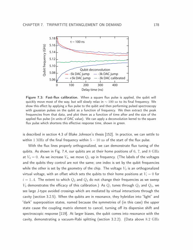
CHAPTER 7. TRIPARTITE ENTANGLEMENT ON DEMAND 178
5.18
5.16
5.14
5.12
5.10
5.08
5.06
Qub
it fr
eque
ncy
(GH
z)
4003002001000Delay time (ns)
~ 100 ns
Qubit deconvolution -5k DAC jump -3k DAC jump +5k DAC jump -3k DAC calibrated
Figure 7.3: Fast-flux calibration. When a square flux pulse is applied, the qubit willquickly move most of the way, but will slowly relax in ∼ 100 ns to its final frequency. Weshow this effect by applying a flux pulse to the qubit and then performing pulsed spectroscopywith gaussian pulses on the qubit as a function of frequency. We then extract the peakfrequencies from that data, and plot them as a function of time after and the size of theapplied flux pulse (in units of DAC value). We can apply a deconvolution kernel to the squareflux pulse which shortens this effective response time, shown in green.
is described in section 4.3 of Blake Johnson’s thesis [152]. In practice, we can settle towithin 1 MHz of the final frequency within 5 − 10 ns of the start of the flux pulse.
With the flux lines properly orthogonalized, we can demonstrate flux tuning of thequbits. As shown in Fig. 7.4, our qubits are at their home positions of 6, 7, and 8 GHz
at V3 = 0. As we increase V3, we move Q1 up in frequency. (The labels of the voltagesand the qubits they control are not the same; one index is set by the qubit frequencieswhile the other is set by the geometry of the chip. The voltage V3 is an orthogonalizedvirtual voltage, with an offset which sets the qubits to their home positions at Vi = 0 fori = 1..4. The extent to which Q2 and Q3 do not change their frequencies as we sweepV3 demonstrates the efficacy of this calibration.) As Q1 tunes through Q2 and Q3, wesee large J-type avoided crossings which are mediated by virtual interactions through thecavity (section 3.2.5). When the qubits are in resonance, they hybridize into “light” and“dark” superposition states, named because the symmetries of (in this case) the upperstate cause the coupling matrix element to cancel, turning off its dispersive shift andspectroscopic response [119]. At larger biases, the qubit comes into resonance with thecavity, demonstrating a vacuum-Rabi splitting (section 3.2.2). (Data above 8.2 GHz
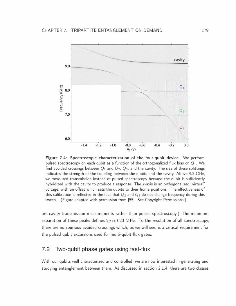
CHAPTER 7. TRIPARTITE ENTANGLEMENT ON DEMAND 179
Figure 7.4: Spectroscopic characterization of the four-qubit device. We performpulsed spectroscopy on each qubit as a function of the orthogonalized flux bias on Q1. Wefind avoided crossings between Q1 and Q2, Q3, and the cavity. The size of these splittingsindicates the strength of the coupling between the qubits and the cavity. Above 8.2 GHz,we measured transmission instead of pulsed spectroscopy because the qubit is sufficientlyhybridized with the cavity to produce a response. The x-axis is an orthogonalized “virtual”voltage, with an offset which sets the qubits to their home positions. The effectiveness ofthis calibration is reflected in the fact that Q2 and Q3 do not change frequency during thissweep. (Figure adapted with permission from [55]. See Copyright Permissions.)
are cavity transmission measurements rather than pulsed spectroscopy.) The minimumseparation of these peaks defines 2g ≈ 620 MHz. To the resolution of all spectroscopy,there are no spurious avoided crossings which, as we will see, is a critical requirement forthe pulsed qubit excursions used for multi-qubit flux gates.
7.2 Two-qubit phase gates using fast-flux
With our qubits well characterized and controlled, we are now interested in generating andstudying entanglement between them. As discussed in section 2.1.4, there are two classes
CHAPTER 7. TRIPARTITE ENTANGLEMENT ON DEMAND 180
of two-qubit gates: controlled-NOT and controlled-phase gates. When the control qubitis in its excited state, the target qubit is flipped around the x-axis (e.g. a bit-flip) by acNOT gate and is flipped around the z-axis (e.g. a phase-flip) by a cPhase gate. Thetwo gates are related to one another with single-qubit pulses – for example, a cPhase isturned into a cNOT by bookending the target qubit with π/2 or Hadamard pulses. Thekey concept is that they are controlled: something happens if and only if the qubits are ina particular state.
There are numerous ways of producing controlled operations in cQED, each with theirown strengths and weaknesses. The primary concern is the ultimate fidelity with whichthe operation can be performed∗. In the case of the four-qubit device, our qubit lifetimeswere only on the order of 1 μs, so fidelity of any operation is well approximated by theT1 decay during its execution. We are therefore interested in using interactions that areas fast (e.g. strong) as possible. We aim to use FBLs to tune interactions terms of thesystem Hamiltonian on and off by moving the qubits together and apart from one another.We will also only consider cPhase gates, which have fewer parameters to calibrate andmore naturally generated in our architecture.
This section will explain two methods of generating controlled-phase gates and entan-glement using fast-flux lines. They exploit an avoided level crossing of non-computationalstates which is accessible only when both qubits are excited, thus providing the conditionalnature of the gate. The first method approaches this crossing adiabatically, which hasthe advantage of being less sensitive to parameters and to compensation of the fluxbias line response function, but is relatively slow. The second approaches the crossingsuddenly, which saves time (and commensurately increases fidelity), but is more technicallychallenging. Both of these techniques will ultimately be used in the next chapter togenerate a three-qubit gate which we use to demonstrate basic quantum error correction.
∗ Other concerns include how easy it is to calibrate the gate, whether it can be trivially repeated (e.g. thesystem has no memory of its application, outside of the qubit states), whether the gate requires extrahardware or engineering either at room temperature or in the device itself, how precisely you need to hitdevice parameters, and so on. In this device, the coherence times were so short that essentially the onlyconcern was gate time, but recently our qubits have become so coherent that we are afforded the luxuryof optimizing for other considerations [169]. Gate fidelities also depend on parameters other than gateduration, though this is often only relevant when qubits are very coherent; this is explored in the citedpaper.
CHAPTER 7. TRIPARTITE ENTANGLEMENT ON DEMAND 181
7.2.1 Adiabatic controlled-phase gate
To generate entanglement, broadly speaking, we require interactions between qubits∗. Basedon the spectroscopy of Fig. 7.4, one obvious place where we would expect interactionsis when they are near resonance with one another other, for example with Q1 and Q2 atV3 = 0.25 V. Indeed, this is a viable way of preparing an entangled state. Imagine that Q2
is initialized in its excited state and Q1 in its ground state (or vice versa) and we quicklymove Q1 into resonance with Q2 with a fast-flux pulse. If we are sudden, the state ofour qubits will not change, but the eigenstates of the Hamiltonian will. That is, thoughwe begin in an energy eigenstate, by changing the Hamiltonian quickly with our fast fluxbias, our wavefunction will no longer be an eigenstate, but rather a mixture of the newlyhybridized eigenbasis. Thus, as a function of time, the excitation that started in Q2 willoscillate between qubits at the rate of the splitting between them. Ideally, this interactionwould produce a J-swap gate, with a unitary⎛⎜⎜⎜⎜⎝
1 0 0 0
0 cos(Jt) isin(Jt) 0
0 isin(Jt) cos(Jt) 0
0 0 0 1
⎞⎟⎟⎟⎟⎠where J is again the interaction strength between the two qubits. If we were to wait forhalf of the oscillation time t = π/4J , we would be left with the excitation half in Q1 andhalf in Q2, giving us a (|01〉 + |10〉) /√2 maximally-entangled Bell state. (Indeed, afterthis section was written, a paper was published that demonstrates the J-swap “gate” [217],and it works exactly as we predicted.) Unfortunately, as we will see, this interaction doesnot work if we start with both qubits simultaneously in their excited states (e.g. the |11〉state); the lower right element of the J-swap unitary is not simply 1. This denigrates theoperation from a true quantum gate (which must work for all inputs) to a method ofpreparing a particular Bell state. It turns out that on the path of Q1 toward Q2, there isan extra interaction that only involves the |11〉 state, which causes this J-swap gate to failbecause quantum amplitude leaks out of the computational Hilbert space.
We can investigate this extra interaction by performing two-tone spectroscopy. Spec-troscopy only detects transitions involving the prepared qubit state (typically the ground
∗ A measurement protocol could also be used, where, for example, the joint properties of the two qubits areinterrogated in such a way that the state is projected onto the Bell basis [218–220].
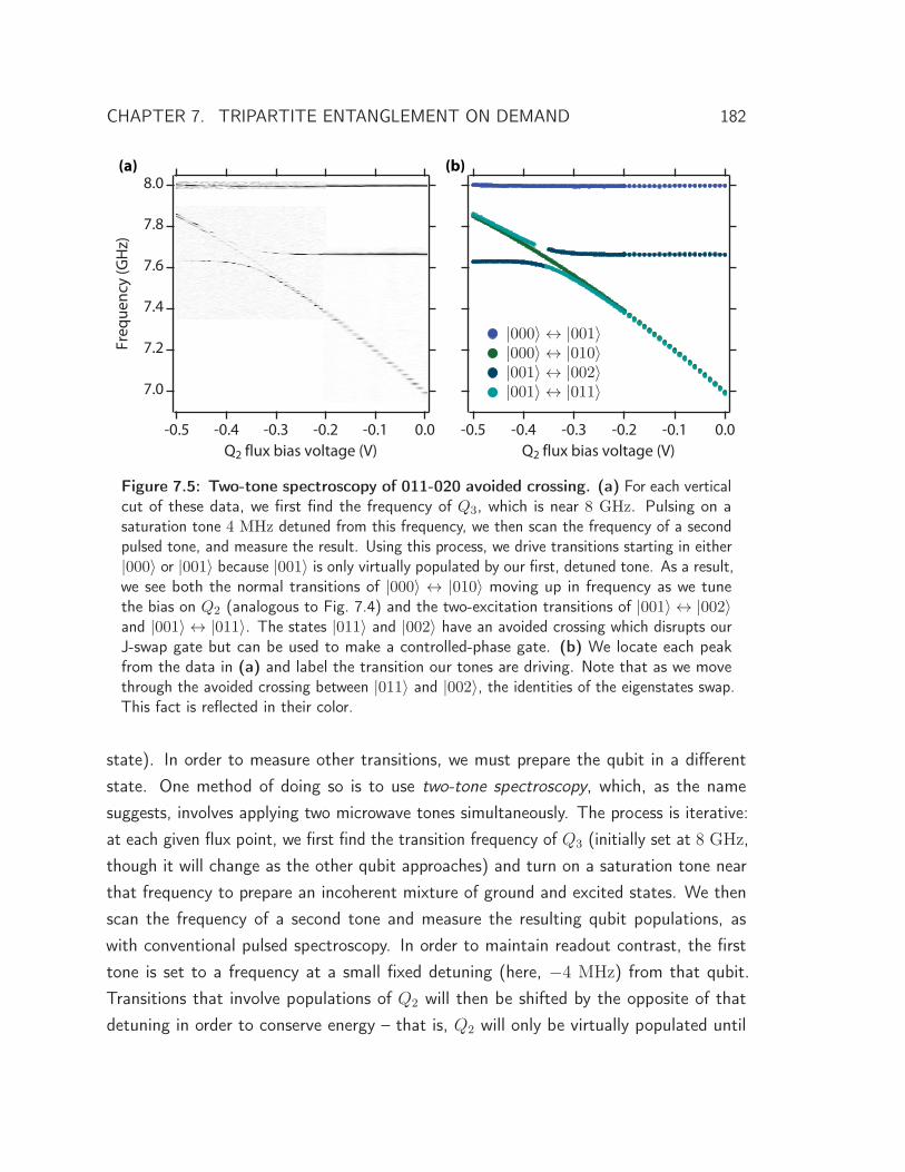
CHAPTER 7. TRIPARTITE ENTANGLEMENT ON DEMAND 182
(a) (b)
|000〉 ↔ |001〉|000〉 ↔ |010〉|001〉 ↔ |002〉|001〉 ↔ |011〉
Figure 7.5: Two-tone spectroscopy of 011-020 avoided crossing. (a) For each verticalcut of these data, we first find the frequency of Q3, which is near 8 GHz. Pulsing on asaturation tone 4 MHz detuned from this frequency, we then scan the frequency of a secondpulsed tone, and measure the result. Using this process, we drive transitions starting in either|000〉 or |001〉 because |001〉 is only virtually populated by our first, detuned tone. As a result,we see both the normal transitions of |000〉 ↔ |010〉 moving up in frequency as we tunethe bias on Q2 (analogous to Fig. 7.4) and the two-excitation transitions of |001〉 ↔ |002〉and |001〉 ↔ |011〉. The states |011〉 and |002〉 have an avoided crossing which disrupts ourJ-swap gate but can be used to make a controlled-phase gate. (b) We locate each peakfrom the data in (a) and label the transition our tones are driving. Note that as we movethrough the avoided crossing between |011〉 and |002〉, the identities of the eigenstates swap.This fact is reflected in their color.
state). In order to measure other transitions, we must prepare the qubit in a differentstate. One method of doing so is to use two-tone spectroscopy, which, as the namesuggests, involves applying two microwave tones simultaneously. The process is iterative:at each given flux point, we first find the transition frequency of Q3 (initially set at 8 GHz,though it will change as the other qubit approaches) and turn on a saturation tone nearthat frequency to prepare an incoherent mixture of ground and excited states. We thenscan the frequency of a second tone and measure the resulting qubit populations, aswith conventional pulsed spectroscopy. In order to maintain readout contrast, the firsttone is set to a frequency at a small fixed detuning (here, −4 MHz) from that qubit.Transitions that involve populations of Q2 will then be shifted by the opposite of thatdetuning in order to conserve energy – that is, Q2 will only be virtually populated until

CHAPTER 7. TRIPARTITE ENTANGLEMENT ON DEMAND 183
the energy deficit is paid by the second tone. (If Q2 were actually populated, we wouldnot see these two-excitation transitions because the difference in measurement contrastbetween whichever final state and |010〉 would likely be small. Our measurement operatoris approximately |000〉〈000|, which does not discriminate between those states.) As aresult, we will also see transitions that start from the qubit in the ground state – essentially,we are turning on sensitivity to extra transitions for free.
The result of this measurement is shown in Fig. 7.5. There, we move Q2 up towardresonance with Q3. We have switched to examining the crossing between Q2 and Q3
instead of Q1 and Q2 because our data for the first case were cleaner; the physics is exactlyanalogous for either pair. We observe the normal single-tone transitions of |000〉 ↔ |010〉(dark green) and |000〉 ↔ |001〉 (blue), but also detect an extra avoided crossing at7.62 GHz and −0.33 V . For small voltages, we see a horizontal line 334 MHz below the|000〉 ↔ |001〉 transition (dark blue). This frequency is exactly the anharmonicity of Q3
(modulo the 4 MHz offset), indicating that this transition is from the first excited stateof Q3 to the second excited state, |001〉 ↔ |002〉. We also observe an extra line that isinitially parallel to |000〉 ↔ |010〉 (teal), but peels off in a crossing with what we nowunderstand to be |002〉. This is the |001〉 ↔ |011〉 transition, and so the avoided crossingis between |011〉 and |002〉. We can now explain why our proposed J-swap gate will notwork: because the qubits have negative anharmonicity, there will always be a large avoidedcrossing between |11x〉 and |02x〉 prior to the |01x〉 ↔ |10x〉 swap. (Recall that weestimated the size of this interaction in section 3.2.5.) If we move through this transitionwith population in |11x〉, we cause quantum amplitude to leak into the non-computationalstate |02x〉. As we will see below, the |11x〉 state will also evolve an additional phasedifference during this process, further distorting it from the ideal J-swap.
Far from being a nuisance as we have characterized it thus far, this extra avoidedcrossing is actually a valuable resource. Consider the energies of the |011〉 state comparedwith the sum of its constituents, |010〉 and |001〉. Initially, as shown in Fig. 7.6(a), the twoenergies will be very similar because we are far from |002〉. As we approach the avoidedcrossing, however, the energy of |011〉 will bend over and lag behind that of |010〉 and|001〉. At this point, the phase evolution of |011〉 will be substantially different than itsconstituents, giving us a conditional phase – evolution that only occurs when both qubitsare excited. We define the difference between the energies of the |011〉 state and itsconstituents to be a parameter ζ, as shown in Fig. 7.6(b).
To explain how we can use this interaction, it is helpful to first write out the unitary
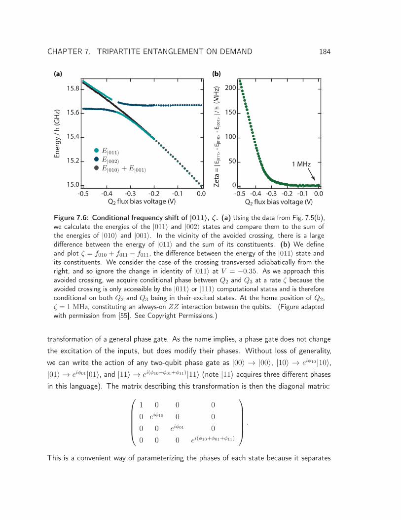
CHAPTER 7. TRIPARTITE ENTANGLEMENT ON DEMAND 184
(a) (b)
1 MHz
E|011〉E|002〉E|010〉 + E|001〉
Figure 7.6: Conditional frequency shift of |011〉, ζ. (a) Using the data from Fig. 7.5(b),we calculate the energies of the |011〉 and |002〉 states and compare them to the sum ofthe energies of |010〉 and |001〉. In the vicinity of the avoided crossing, there is a largedifference between the energy of |011〉 and the sum of its constituents. (b) We defineand plot ζ = f010 + f011 − f011, the difference between the energy of the |011〉 state andits constituents. We consider the case of the crossing transversed adiabatically from theright, and so ignore the change in identity of |011〉 at V = −0.35. As we approach thisavoided crossing, we acquire conditional phase between Q2 and Q3 at a rate ζ because theavoided crossing is only accessible by the |011〉 or |111〉 computational states and is thereforeconditional on both Q2 and Q3 being in their excited states. At the home position of Q2,ζ = 1 MHz, constituting an always-on ZZ interaction between the qubits. (Figure adaptedwith permission from [55]. See Copyright Permissions.)
transformation of a general phase gate. As the name implies, a phase gate does not changethe excitation of the inputs, but does modify their phases. Without loss of generality,we can write the action of any two-qubit phase gate as |00〉 → |00〉, |10〉 → eiφ10 |10〉,|01〉 → eiφ01 |01〉, and |11〉 → ei(φ10+φ01+φ11)|11〉 (note |11〉 acquires three different phasesin this language). The matrix describing this transformation is then the diagonal matrix:⎛⎜⎜⎜⎜⎝
1 0 0 0
0 eiφ10 0 0
0 0 eiφ01 0
0 0 0 ei(φ10+φ01+φ11)
⎞⎟⎟⎟⎟⎠ .
This is a convenient way of parameterizing the phases of each state because it separates
CHAPTER 7. TRIPARTITE ENTANGLEMENT ON DEMAND 185
the origins of each phase. The first two, φ10 and φ01, are known as single-qubit phases,and as we will see are due to the trivial phase evolution of any one qubit. φ11, on theother hand, is a two-qubit phase, which is a phase evolution that occurs only when bothqubits are exited and is associated with two-qubit interactions and entanglement. Thisparametrization properly distributes phases; if we did a z-gate on a single qubit such thatφ10 = π, any state with the first qubit excited (that is, both |10〉 and |11〉) should haveits phase flipped and we would have the unitary diag{1,−1, 1,−1}∗.
Let us first consider how we would get a “single-qubit” phase. The quantum amplitudeof a state with energy E = �ω0 evolves proportional to eiω0t. This evolution is normallyeliminated because we work in the rotating frame of an RF generator tuned to the qubittransition frequency. However, if the qubit were to be detuned from its reference framewith a flux pulse, the difference between the qubit’s instantaneous energy and its referencewould be responsible for a phase evolution. As a function of time, the overall phase delaywould be given by φsq =
∫ t
0(ω0 − ω(τ))dτ =
∫ t
0Δ(τ)dτ . It is worth noting that to control
a single-qubit phase, we do not actually need to change the associated qubit’s frequency.It is only defined relative to the rotating frame of its respective drive, so we need onlyadvance or retard the phase of that oscillator to control it. This is easily done in softwareby changing what defines the x- and y-axes for all pulses following a “virtual” z-gate, whichcomes down to changing the distribution of voltages on the I and Q ports of our mixer.The fact that we are free to do this reveals the triviality of these single-qubit phases.
In contrast, a two-qubit phase is a more subtle beast that can have real physicalimplications. As you may have anticipated, one way of acquiring such a two-qubit phaseinvolves the avoided crossing between |11〉 and |02〉. As we have defined it above, thetwo-qubit phase is the difference in phase between |11〉 and its constituents. Thus, wewill acquire conditional phase at a rate proportional to the difference in energy between|11〉 and the sum of |10〉 and |01〉. Having previously defined this quantity as ζ, if weagain tune Q2’s frequency over some trajectory, the conditional phase acquired would beφ11 =
∫ t
0ζ(τ)dτ . Importantly, two-qubit phases are phase differences between qubits and
cannot be generated in software†. Multi-qubit phase is very precious!We have thus far neglected to emphasize that this mechanism relies on all of our flux
∗ Note that our definition of single- and two-qubit phases is slightly different than the one found in Ref. 121.† We can make an analogy between qubit phases and potential energies. Physically, the only thing that
matters is the energy difference between a starting and ending state of some process. We are free torenormalize an energy scale to whatever convenient zero we choose. This is similar with phases: a
CHAPTER 7. TRIPARTITE ENTANGLEMENT ON DEMAND 186
pulses being adiabatic to the avoided crossing. Adiabatic means that our qubit alwaysremains in an instantaneous eigenstate of the time-dependent Hamiltonian. This is onlyan issue when there are avoided level crossings, where eigenstates mix and change identity.If we approach these splittings slowly enough, our wavefunction will evolve exactly withthe changing eigenstate and stay on the same energy “track.” The timescale (or, energychange per unit of time) that we must be slow compared to is determined by the sizeof the splitting. “Slow” depends on the details of the Hamiltonian, but in practice ourapproach must take a few times longer than the splitting period. The larger the avoidedcrossing, the easier it is to be adiabatic to it. The more closely you approach a crossing,the slower you must be to inhibit undesired tunneling. Optimally acquiring two-qubit phaseis a matter of finding the best trade-off between the magnitude of ζ and speed; the largerζ, the slower our trajectory must be. The best solution is one in which you never stopmoving the qubit, since any stationary time would be cut down by bringing the qubit closerto the crossing.
With our source of two-qubit phase established, we can now construct a cPhase gate.The canonical conditional-phase gate is, as mentioned earlier, one which flips the phaseof the qubit manifold if and only if both qubits are excited∗. Thus, the unitary matrixshould be diag{1, 1, 1,−1} and we can immediately see that we need φ10 = φ01 = 0 andφ11 = π. To get the two-qubit phase, we apply a flux pulse that tunes the qubits close toone another (where ζ is large) while maintaining our adiabaticity to the avoided crossing.We can fine-tune the time and amplitude of the pulse to satisfy φ11 =
∫ t
0ζ(τ)dτ = π.
This conditional phase can be measured by applying a Ramsey sequence on one qubitwhile preparing the other in either its ground or excited state. (This “conditional Ramsey”experiment is very useful whenever you are interested in measuring conditional phaseevolution and will be discussed in more detail in section 8.1.5.) We satisfy our conditionwhen the resulting oscillations are exactly π out of phase from one another. During theflux pulse, we will also get large single-qubit phases, since the qubits will be detuned fromtheir phase references. These are no problem, though, because we can simply measurethem (using a procedure similar to that for two-qubit phases, where instead of toggling
single-qubit phase is like an energy that can be arbitrarily changed in our book-keeping, while a two-qubitphase is an energy difference that has physical implications.
CHAPTER 7. TRIPARTITE ENTANGLEMENT ON DEMAND 187
the excitation of one of the qubits we measure the qubit phase with and without the gateapplied) and unwrap them in software.
There are four equivalent cPhase gates, differing only by which computational statepicks up the −1 sign. All the gates have π conditional phase, but differ in their valuesof single-qubit phase. For example, if we wished to put the −1 sign on the ground state,we would set φ10 = φ01 = π, in addition to φ11 = π (in this case we have the matrixdiag{1,−1,−1,−1} which is equal to diag{−1, 1, 1, 1} when we factor out a globalphase). Similarly, we can move the minus sign to |10〉 by setting φ10 = π and φ01 = 0 orput it on |01〉 with the opposite configuration. These gates are not different evolutionssince we can apply our z-gates in software. Instead, you should consider them to be ameans of keeping track of the single-qubit phase evolution that may be necessary to createa particular quantum state.
An adiabatic cPhase gate was used in the first demonstration of on-demand entangle-ment and quantum algorithms with superconducting qubits [121]. It has the advantage ofbeing straightforward to tune-up and insensitive both to pulse timings and flux trajectory.However, it is relatively slow because we must be adiabatic to the qubit-qubit interactionwe are using to generate conditional phase. These gates typically take about 30 − 40 ns,which is several times the 10− 15 ns splitting period. Since the coherence time of thesedevices was so low, this inefficiency is undesirable. Fortunately, there is another version ofthis gate that operates at full speed which we describe in the next section.
7.2.2 Sudden controlled-phase gate
Now that we have explored what happens when approaching the |11〉 ↔ |02〉 avoidedcrossing adiabatically, it is interesting to consider the case of moving suddenly. This is theopposite limit, where we move so fast that our state wavefunction does not have a chanceto evolve in response to the changing Hamiltonian. In the vicinity of the avoided crossing,where eigenstates change their identities, our wavefunction will become a hybridization
∗ There is no sense of individual “target” or “control” qubits with a cPhase gate. Each computational basisstate has only one phase degree of freedom and only |11〉 gets the extra phase. Each qubit thereforeacts as both a control and a target. This is in contrast to the controlled-NOT gate, where each qubitcan individually flip and the gate can transmute one basis state to another. Since a phase-flip gate canbe easily converted to a bit-flip gate and vice versa, there is no substantive meaning underlying thisasymmetry – it is just an artifact of the basis we choose for computation. This fact is the origin of theidea of a “phase kickback” and can complicate the interpretation of a quantum circuit diagram if you arenot looking for it.
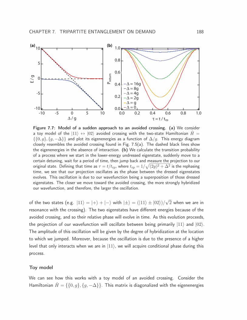
CHAPTER 7. TRIPARTITE ENTANGLEMENT ON DEMAND 188
Δ τ
ΔΔΔΔΔΔ
(a) (b)
Figure 7.7: Model of a sudden approach to an avoided crossing. (a) We considera toy model of the |11〉 ↔ |02〉 avoided crossing with the two-state Hamiltonian H ={{0, g}, {g,−Δ}} and plot its eigenenergies as a function of Δ/g. This energy diagramclosely resembles the avoided crossing found in Fig. 7.5(a). The dashed black lines showthe eigenenergies in the absence of interaction. (b) We calculate the transition probabilityof a process where we start in the lower-energy undressed eigenstate, suddenly move to acertain detuning, wait for a period of time, then jump back and measure the projection to ouroriginal state. Defining that time as τ = t/trp, where trp = 1/
√(2g)2 +Δ2 is the rephasing
time, we see that our projection oscillates as the phase between the dressed eigenstatesevolves. This oscillation is due to our wavefunction being a superposition of those dressedeigenstates. The closer we move toward the avoided crossing, the more strongly hybridizedour wavefunction, and therefore, the larger the oscillation.
of the two states (e.g. |11〉 = |+〉 + |−〉 with |±〉 = (|11〉 ± |02〉)/√2 when we are inresonance with the crossing). The two eigenstates have different energies because of theavoided crossing, and so their relative phase will evolve in time. As this evolution proceeds,the projection of our wavefunction will oscillate between being primarily |11〉 and |02〉.The amplitude of this oscillation will be given by the degree of hybridization at the locationto which we jumped. Moreover, because the oscillation is due to the presence of a higherlevel that only interacts when we are in |11〉, we will acquire conditional phase during thisprocess.
Toy model
We can see how this works with a toy model of an avoided crossing. Consider theHamiltonian H = {{0, g}, {g,−Δ}}. This matrix is diagonalized with the eigenenergies

CHAPTER 7. TRIPARTITE ENTANGLEMENT ON DEMAND 189
E± =(±√(2g)2 +Δ2 − Δ
)/2, as plotted in Fig. 7.7(a), and has associated eigenvectors
v± = {cos (θ±m) , sin (θ±m)} with θ±m = cot−1
(2g
Δ±√
(2g)2+Δ2
). If we start far detuned from
the crossing, with Δ → ∞, we have v− ≈ {0, 1} and E− ≈ −Δ. We are interested inwhat happens when we suddenly jump to a certain detuning and wait for some period oftime. The operator describing this evolution is given by
U = |v+〉〈v+|eiE+t/h + |v−〉〈v−|eiE−t/h (7.1)
where we evaluate the eigenvectors and eigenenergies at the Δ to which we are jumping.Starting in a pure state |v0〉 = {0, 1}, we say the probability that we return to ourinitial state is given by Preturn (t,Δ, g) = |〈v0|U |v0〉|2. The “rephasing” time, defined bythe first time that Preturn (trp,Δ, g) = 1 and physically corresponding to one full periodof oscillation, is given by trp = 1/
√(2g)2 +Δ2. Defining τ = t/trp, we can plot this
return probability as a function of time for several values of Δ, shown in Fig. 7.7(b). Asanticipated, the amplitude of this oscillation is given by the degree of hybridization; farfrom the avoided crossing, there is very little transfer of population, while in resonance thestate is fully transferred to the other eigenstate and back.
What is the conditional phase acquired during this process? One thing that is initiallyconfusing is that if we calculate the phase angle of 〈v0|U |v0〉 at t = trp, we get φ0 =
−π
(1 + Δ√
(2g)2+Δ2
). Does that mean we are getting more than π of two-qubit phase
when we wait off-resonance and so are maximally entangled at some intermediate time?The answer is no – we actually acquire less conditional phase for finite Δ – but to seethat we must consider what would happen if the avoided crossing were not there. Wehave added dashed lines alongside the eigenenergies plotted in Fig. 7.7(a) to indicate theenergies for the case of no interaction between the states. This is our analog for theenergies of the constituent computational states in the adiabatic case described in theprevious section; it defines the single-qubit phase that we must subtract to determine ourconditional phase. The phase acquired by this state is given by φ1 = Eg=0
− t = −2πΔt. Ifwe consider only the times that cause full oscillations, we have φ1 = −2πΔtrp = −2πΔ√
(2g)2+Δ2.
Our conditional phase is then φc = φ0 − φ1 = π
(1 − Δ√
(2g)2+Δ2
). This has the expected
limits of φc → 0 as Δ → −∞ and φc = π when Δ = 0. We show the behavior of thetwo-qubit phase as a function of time and Δ (at t = trp) in Fig. 7.8.
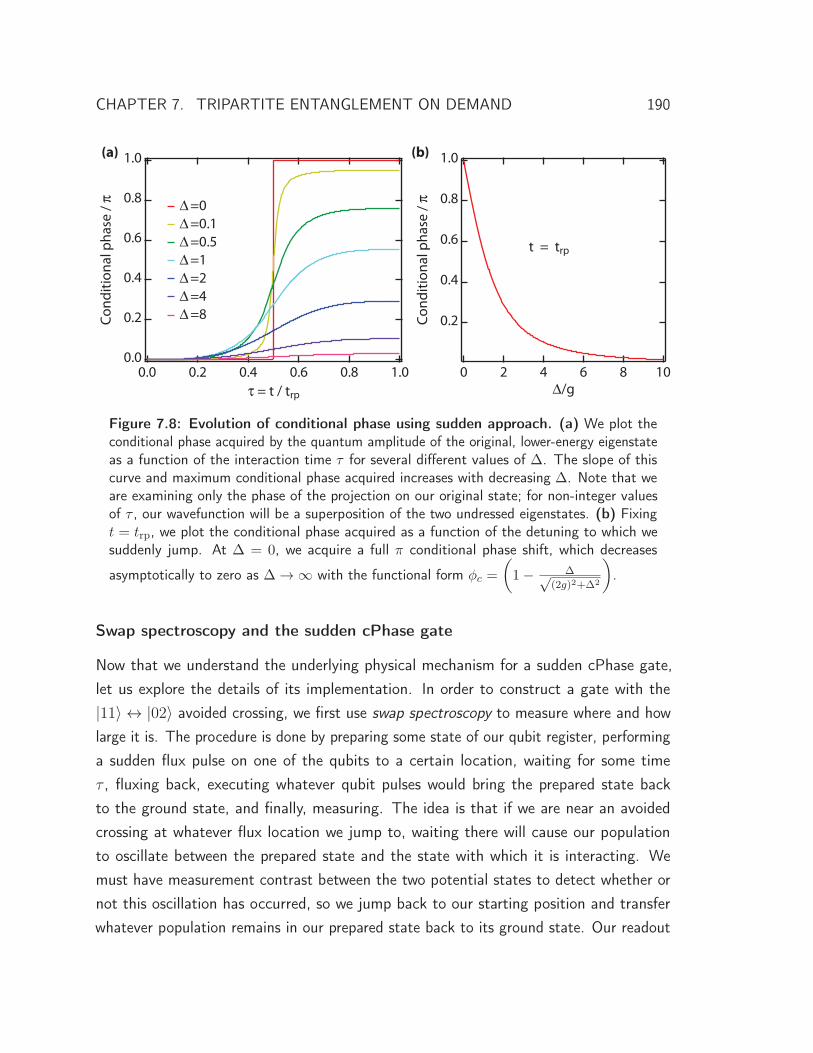
CHAPTER 7. TRIPARTITE ENTANGLEMENT ON DEMAND 190
π
Δ
π
τ
Δ Δ Δ Δ Δ Δ Δ
(a) (b)
Figure 7.8: Evolution of conditional phase using sudden approach. (a) We plot theconditional phase acquired by the quantum amplitude of the original, lower-energy eigenstateas a function of the interaction time τ for several different values of Δ. The slope of thiscurve and maximum conditional phase acquired increases with decreasing Δ. Note that weare examining only the phase of the projection on our original state; for non-integer valuesof τ , our wavefunction will be a superposition of the two undressed eigenstates. (b) Fixingt = trp, we plot the conditional phase acquired as a function of the detuning to which wesuddenly jump. At Δ = 0, we acquire a full π conditional phase shift, which decreases
asymptotically to zero as Δ → ∞ with the functional form φc =
(1 − Δ√
(2g)2+Δ2
).
Swap spectroscopy and the sudden cPhase gate
Now that we understand the underlying physical mechanism for a sudden cPhase gate,let us explore the details of its implementation. In order to construct a gate with the|11〉 ↔ |02〉 avoided crossing, we first use swap spectroscopy to measure where and howlarge it is. The procedure is done by preparing some state of our qubit register, performinga sudden flux pulse on one of the qubits to a certain location, waiting for some timeτ , fluxing back, executing whatever qubit pulses would bring the prepared state backto the ground state, and finally, measuring. The idea is that if we are near an avoidedcrossing at whatever flux location we jump to, waiting there will cause our populationto oscillate between the prepared state and the state with which it is interacting. Wemust have measurement contrast between the two potential states to detect whether ornot this oscillation has occurred, so we jump back to our starting position and transferwhatever population remains in our prepared state back to its ground state. Our readout
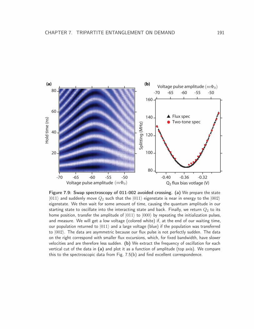
CHAPTER 7. TRIPARTITE ENTANGLEMENT ON DEMAND 191
(mΦ0)
(mΦ0)(a) (b)
Figure 7.9: Swap spectroscopy of 011-002 avoided crossing. (a) We prepare the state|011〉 and suddenly move Q2 such that the |011〉 eigenstate is near in energy to the |002〉eigenstate. We then wait for some amount of time, causing the quantum amplitude in ourstarting state to oscillate into the interacting state and back. Finally, we return Q2 to itshome position, transfer the amplitude of |011〉 to |000〉 by repeating the initialization pulses,and measure. We will get a low voltage (colored white) if, at the end of our waiting time,our population returned to |011〉 and a large voltage (blue) if the population was transferredto |002〉. The data are asymmetric because our flux pulse is not perfectly sudden. The dataon the right correspond with smaller flux excursions, which, for fixed bandwidth, have slowervelocities and are therefore less sudden. (b) We extract the frequency of oscillation for eachvertical cut of the data in (a) and plot it as a function of amplitude (top axis). We comparethis to the spectroscopic data from Fig. 7.5(b) and find excellent correspondence.

CHAPTER 7. TRIPARTITE ENTANGLEMENT ON DEMAND 192
will then discriminate between the qubit in the ground state (indicating that no leakagehas occurred) and the qubit in some other state that it tunneled into during the waitingtime.
In Fig. 7.9(a) we show the result of performing swap spectroscopy on the |110〉 ↔ |020〉avoided crossing when preparing |110〉. We observe the characteristic “chevron” pattern ofa suddenly-approached avoided crossing. We plot the measurement result as a function ofboth flux pulse amplitude and the time we hold at each applied voltage. Where we get arelatively small voltage, indicated in white, the qubit’s wavefunction is unchanged; a darkpixel corresponds to a large voltage and population transfer to |020〉. The frequency ofthis oscillation corresponds well with the prediction from our simple model. The frequencyof oscillation is minimal (86 MHz) when we move into resonance with the avoided crossing(V = −55 mΦ0). As we detune, the frequency increases according to f =
√(2g)2 +Δ2.
The amplitude of oscillation also decreases in a similar way. In Fig. 7.9(a) we plot theoscillation frequency extracted from the chevron data (top and right axes) and overlaythe spectroscopically measured splittings from Fig. 7.6 (bottom and left axes), showingexcellent correspondence between the two methods. Flux spectroscopy is much moreprecise since we have the luxury of fitting a sinusoid rather than two Lorentzians.
With this information, it is simple to construct our cPhase gate. The amplitude ofour flux pulse is given by the voltage corresponding to the slowest oscillation frequencywe found in swap spectroscopy, V ≈ 55 mΦ0. (Note that we have converted to units ofΦ0 to have physical meaning, but experimentally we specify a voltage amplitude.) Weapply a square flux pulse with the fastest possible rise time to be maximally sudden for atime of t = 1/f ∼ 12 ns, where f = 86 MHz is the splitting of the avoided crossing. Aswith the adiabatic case, we must also measure and correct single-qubit phases in software.The resulting gate is of relatively high fidelity owing to its fast speed, as we will see insection 7.4.
One potential concern is whether we are able to precisely time our excursion, sinceany error would cause some leakage into |020〉. We can be neither perfectly sudden, norcan we exactly hit the timing of 11.62 ns corresponding to one oscillation. While thereare methods of detecting and compensating for these small timing errors (discussed insection 8.1.2), for the purposes of a cPhase gate on qubits with relatively short T1s, theseerrors are negligible enough to disregard.
CHAPTER 7. TRIPARTITE ENTANGLEMENT ON DEMAND 193
7.2.3 Other two-qubit gates
The adiabatic and sudden fluxed cPhase gates that we have discussed are by no meansthe only methods of generating entanglement in cQED. In fact, though they were the firstpractical gates demonstrated, they will almost certainly not represent the best approachgoing forward. Our ideal gate is fast (as these are), but also has high “intrinsic” gatefidelity and does not require additional hardware in the device or at room temperature.The intrinsic gate fidelity is a vague term which refers, in this context, to the infidelityof the gate unrelated to T1 or T2. For example, non-adiabaticity or timing errors mightcause leakage into the |02x〉 state, the size of which directly reduces the gate’s fidelity.These errors are also quite insidious, because they would not be corrected by most formsof quantum error correction [221]. More importantly, these gates require fast flux lines. Inaddition to requiring an extra cryogenic microwave line and room temperature electronics,making the qubits sensitive to flux inexorably decreases their T2 coherence times becauseof flux noise.
One appealing gate that we have recently developed [169] works by utilizing thedispersive shift of the cavity frequency – exactly the same mechanism used in qubit readout.We adiabatically apply a microwave pulse far detuned from the cavity such that the cavitystate is instantaneously proportional to the drive state, and turn it on and off slowly so thatthe cavity returns to its ground state. Each dispersively shifted cavity will take a differenttrajectory in Hilbert space and therefore will acquire a different phase (of both geometricand Stark-shift origins). Decomposing these phases into single- and two-qubit types, wecan tune-up a cPhase gate in the same way as normal. This gate is interesting becauseit only requires microwave tones on the cavity – something we automatically have forperforming readout – and has high intrinsic fidelity. The two main sources – measurementinduced dephasing and non-adiabaticity – can be made extremely small with appropriatechoice of device parameters.
There are other attractive microwave-only gates that have been developed [222–224],including the Bell-Rabi gate [176] that directly drives the |00〉 ↔ |11〉 transition, and thecross-resonance gate [209], which relies on a state-dependent Rabi rate of the two qubits.This is by no means an exhaustive list; indeed, superconducting qubits in cQED seem tolove entangling with one another since they have large spatial wave functions. Ratherthan being difficult to entangle, in fact, it seems that the challenge in moving toward
CHAPTER 7. TRIPARTITE ENTANGLEMENT ON DEMAND 194
high-fidelity gates will be to make sure the qubits do not unintentionally entangle with oneanother.
7.3 State tomography
Now that we have the ability to generate entanglement, how can we prove that we have doneso? If we are given many copies of some unknown state, how can we determine what thatstate is? The act of reconstructing the density matrix from an ensemble of states is calledstate tomography. Constructing a state tomogram involves measuring some property of aquantum state; by averaging the result of that and other measurements over an ensembleof identically prepared states, we can infer every entry of the matrix. We can express an N
qubit density matrix as a sum of Pauli correlations times their associated operator. For a sin-gle qubit, we have ρ = 1
2
∑tr (ρI) + tr (ρX)X + tr (ρY )Y + tr (ρZ)Z. We define the
quantity 〈O〉 ≡ tr(ρO). This generalizes, for N qubits, to ρ = 1
2N
∑O∈{I⊗N ..Z⊗N}〈O〉O
where the sum is taken over every N -qubit Pauli operator∗. Thus, reconstructing thedensity matrix is the same as knowing each of the quantities 〈O〉.
The most conceptually straightforward way to measure these Pauli correlations is withsingle-shot single-qubit measurements. If we have the ability to measure 〈O〉 for eachqubit individually, we can calculate the correlations in software with classical processing.For example, we would find 〈ZZ〉 by calculating the probability that, when we measuredthe Z projection of both qubits at the same time, we found that both pointed in thesame direction, and subtract from that the probability that they were both pointingin the opposite direction. Similarly, calculating quantities such as 〈XY 〉 would requiremeasuring the X projection of Q1 simultaneous with the Y projection of Q2. In our system,however, we do not have the capability of measuring each qubit individually. Instead,our measurement operator (under normal circumstances) is one which projects the qubitmanifold to the ground state: M = |0⊗N〉〈0⊗N |. We get a 0 if all the qubits are in theirground state, and a 1 otherwise. Taking the case of two qubits, we can express thisoperator in terms of Pauli operators as M2 = |00〉〈00| = (II + ZI + IZ + ZZ) /4, where
∗ For example, for two qubits there are 16 Pauli operators: II, XI, Y I, ZI, IX, IY , IZ, XX, Y X,ZX, XY , Y Y , ZY ,XZ, Y Z, and ZZ. For three qubits there are 64, and for N , there are 4N . That is,the amount of information stored in a manifold of qubits grows exponentially with the number N . Thenotation I⊗N denotes the tensor product of N Pauli I operators, e.g. I...I.
CHAPTER 7. TRIPARTITE ENTANGLEMENT ON DEMAND 195
Z is the Pauli z matrix∗. We see in this representation that our measurement operatorinexorably projects all of them.
This measurement operator is actually ideal for tomography because it eliminates theneed for single-shot measurements and for manually calculating correlations. Considerwhat would happen if we performed qubit rotations – say, a π pulse on the first qubit –just prior to measuring. If we view that π pulse as acting on the measurement operatorrather than the qubit state, we would flip all of the Z correlations of the second qubit,making M
R1π
2 = II − ZI + IZ − ZZ. If we instead were to pulse only the secondqubit, we would have M
R2π
2 = II + ZI − IZ − ZZ. Taking the sum of the ensembleaveraged values of these two cases, we would have 〈MR1
π2 〉 + 〈MR2
π2 〉 = 〈II〉 − 〈ZI〉 +
〈IZ〉 − 〈ZZ〉 + 〈II〉 + 〈ZI〉 − 〈IZ〉 − 〈ZZ〉 = 2〈II〉 − 2〈ZZ〉. Since 〈II〉 ≡ 1, wecan directly calculate 〈ZZ〉 = 1
2
(2 − 〈MR1
π2 〉 − 〈MR2
π2 〉
). Thus, by performing rotations
on the ensemble immediately prior to measurement, we can calculate any single-qubit ortwo-qubit correlation with linear combinations of our measurement results.
The measurement operator is actually more complicated than∣∣0⊗N
⟩⟨0⊗N
∣∣ because offinite measurement fidelity and differing sensitivity to the various basis states. For example,recalling the case of multi-qubit readout with the high-power Jaynes-Cummings readoutmechanism described in section 6.3.2, we had ∼ 67% fidelity to the least-distinguishable|100〉 state, but in excess of 80% fidelity to others. This disparity could have been madeeven more extreme had we optimized for a state other than |100〉: the difference in fidelitycould be two-to-one or more. Taken in the ensemble, we will measure slightly differentvoltages for each basis state. (Indeed, if we are in an eigenstate and given enough averaging,we can know not just whether or not we have the ground state, but also exactly whatstate we are in.) Since our experiment gives us voltages and not measurement operatorexpectation values, we must compensate for this fact.
One simple way of calibrating the differing sensitivity to basis states is to modifyour Pauli expansion of the measurement operator. Rather than saying that M2 =
(II + ZI + IZ + ZZ) /2, we add coefficients in front of each term of the operatorand take the ensemble average such that our measurement voltage is given by V M
2 ≡
∗ The operator |00〉〈00| =(
1 0 0 00 0 0 00 0 0 00 0 0 0
)if we assume the qubit amplitude is confined to the computational
subspace. We have II =
(1 0 0 00 1 0 00 0 1 00 0 0 1
), ZI =
(1 0 0 00 −1 0 00 0 1 00 0 0 −1
), IZ =
(1 0 0 00 1 0 00 0 −1 00 0 0 −1
), and ZZ =
(1 0 0 00 −1 0 00 0 −1 00 0 0 1
).
Thus |00〉〈00| = (II + IZ + ZI + ZZ) /4. Similarly, the measurement operator for three qubits M3 =|000〉〈000| = III + ZII + IZI + IIZ + ZZI + ZIZ + IZZ + ZZZ, and so on for more qubits.
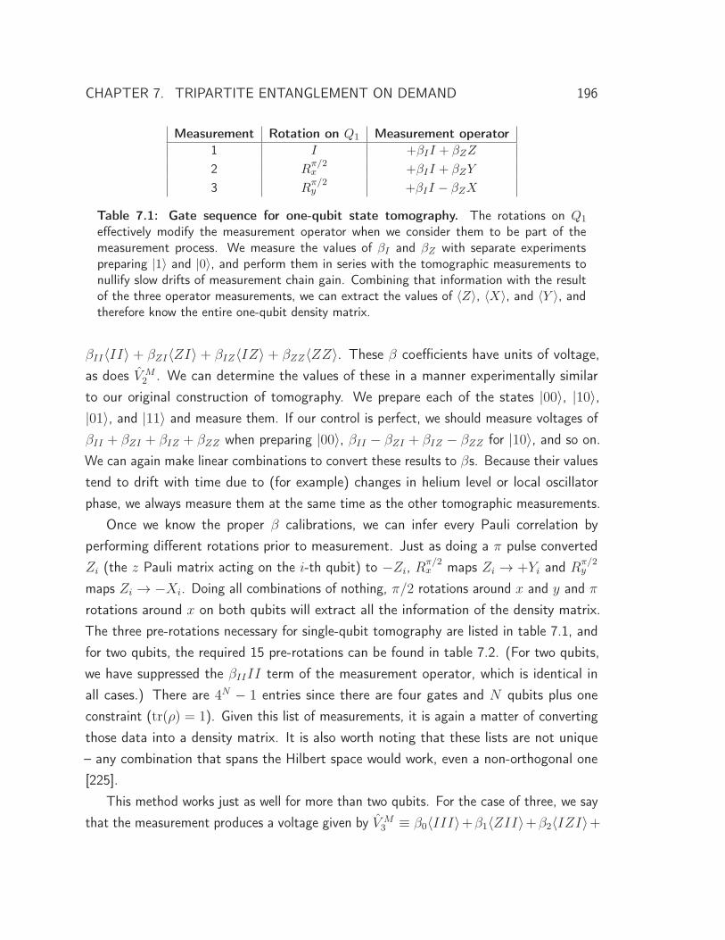
CHAPTER 7. TRIPARTITE ENTANGLEMENT ON DEMAND 196
Measurement Rotation on Q1 Measurement operator1 I +βII + βZZ
2 Rπ/2x +βII + βZY
3 Rπ/2y +βII − βZX
Table 7.1: Gate sequence for one-qubit state tomography. The rotations on Q1
effectively modify the measurement operator when we consider them to be part of themeasurement process. We measure the values of βI and βZ with separate experimentspreparing |1〉 and |0〉, and perform them in series with the tomographic measurements tonullify slow drifts of measurement chain gain. Combining that information with the resultof the three operator measurements, we can extract the values of 〈Z〉, 〈X〉, and 〈Y 〉, andtherefore know the entire one-qubit density matrix.
βII〈II〉 + βZI〈ZI〉 + βIZ〈IZ〉 + βZZ〈ZZ〉. These β coefficients have units of voltage,as does V M
2 . We can determine the values of these in a manner experimentally similarto our original construction of tomography. We prepare each of the states |00〉, |10〉,|01〉, and |11〉 and measure them. If our control is perfect, we should measure voltages ofβII + βZI + βIZ + βZZ when preparing |00〉, βII − βZI + βIZ − βZZ for |10〉, and so on.We can again make linear combinations to convert these results to βs. Because their valuestend to drift with time due to (for example) changes in helium level or local oscillatorphase, we always measure them at the same time as the other tomographic measurements.
Once we know the proper β calibrations, we can infer every Pauli correlation byperforming different rotations prior to measurement. Just as doing a π pulse convertedZi (the z Pauli matrix acting on the i-th qubit) to −Zi, R
π/2x maps Zi → +Yi and R
π/2y
maps Zi → −Xi. Doing all combinations of nothing, π/2 rotations around x and y and π
rotations around x on both qubits will extract all the information of the density matrix.The three pre-rotations necessary for single-qubit tomography are listed in table 7.1, andfor two qubits, the required 15 pre-rotations can be found in table 7.2. (For two qubits,we have suppressed the βIIII term of the measurement operator, which is identical inall cases.) There are 4N − 1 entries since there are four gates and N qubits plus oneconstraint (tr(ρ) = 1). Given this list of measurements, it is again a matter of convertingthose data into a density matrix. It is also worth noting that these lists are not unique– any combination that spans the Hilbert space would work, even a non-orthogonal one[225].
This method works just as well for more than two qubits. For the case of three, we saythat the measurement produces a voltage given by V M
3 ≡ β0〈III〉+β1〈ZII〉+β2〈IZI〉+
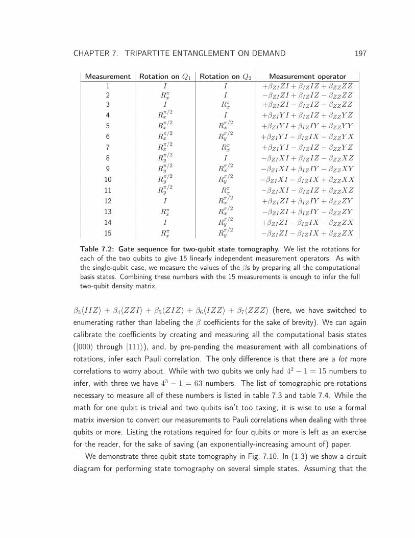
CHAPTER 7. TRIPARTITE ENTANGLEMENT ON DEMAND 197
Measurement Rotation on Q1 Rotation on Q2 Measurement operator1 I I +βZIZI + βIZIZ + βZZZZ2 Rπ
x I −βZIZI + βIZIZ − βZZZZ3 I Rπ
x +βZIZI − βIZIZ − βZZZZ
4 Rπ/2x I +βZIY I + βIZIZ + βZZY Z
5 Rπ/2x R
π/2x +βZIY I + βIZIY + βZZY Y
6 Rπ/2x R
π/2y +βZIY I − βIZIX − βZZY X
7 Rπ/2x Rπ
x +βZIY I − βIZIZ − βZZY Z
8 Rπ/2y I −βZIXI + βIZIZ − βZZXZ
9 Rπ/2y R
π/2x −βZIXI + βIZIY − βZZXY
10 Rπ/2y R
π/2y −βZIXI − βIZIX + βZZXX
11 Rπ/2y Rπ
x −βZIXI − βIZIZ + βZZXZ
12 I Rπ/2x +βZIZI + βIZIY + βZZZY
13 Rπx R
π/2x −βZIZI + βIZIY − βZZZY
14 I Rπ/2y +βZIZI − βIZIX − βZZZX
15 Rπx R
π/2y −βZIZI − βIZIX + βZZZX
Table 7.2: Gate sequence for two-qubit state tomography. We list the rotations foreach of the two qubits to give 15 linearly independent measurement operators. As withthe single-qubit case, we measure the values of the βs by preparing all the computationalbasis states. Combining these numbers with the 15 measurements is enough to infer the fulltwo-qubit density matrix.
β3〈IIZ〉 + β4〈ZZI〉 + β5〈ZIZ〉 + β6〈IZZ〉 + β7〈ZZZ〉 (here, we have switched toenumerating rather than labeling the β coefficients for the sake of brevity). We can againcalibrate the coefficients by creating and measuring all the computational basis states(|000〉 through |111〉), and, by pre-pending the measurement with all combinations ofrotations, infer each Pauli correlation. The only difference is that there are a lot morecorrelations to worry about. While with two qubits we only had 42 − 1 = 15 numbers toinfer, with three we have 43 − 1 = 63 numbers. The list of tomographic pre-rotationsnecessary to measure all of these numbers is listed in table 7.3 and table 7.4. While themath for one qubit is trivial and two qubits isn’t too taxing, it is wise to use a formalmatrix inversion to convert our measurements to Pauli correlations when dealing with threequbits or more. Listing the rotations required for four qubits or more is left as an exercisefor the reader, for the sake of saving (an exponentially-increasing amount of) paper.
We demonstrate three-qubit state tomography in Fig. 7.10. In (1-3) we show a circuitdiagram for performing state tomography on several simple states. Assuming that the

CHAPTER 7. TRIPARTITE ENTANGLEMENT ON DEMAND 198
# RQ1 RQ2 RQ3 Measurement operator1 I I I +β1ZII+β2IZI+β3IIZ+β4ZZI+β5ZIZ+β6IZZ+β7ZZZ
2 I I Rπ/2x +β1ZII+β2IZI+β3IIY+β4ZZI+β5ZIY+β6IZY+β7ZZY
3 I I Rπ/2y +β1ZII+β2IZI−β3IIX+β4ZZI−β5ZIX−β6IZX−β7ZZX
4 I I Rπx +β1ZII+β2IZI−β3IIZ+β4ZZI−β5ZIZ−β6IZZ−β7ZZZ
5 I Rπ/2x I +β1ZII+β2IY I+β3IIZ+β4ZY I+β5ZIZ+β6IY Z+β7ZY Z
6 I Rπ/2x R
π/2x +β1ZII+β2IY I+β3IIY+β4ZY I+β5ZIY+β6IY Y+β7ZY Y
7 I Rπ/2x R
π/2y +β1ZII+β2IY I−β3IIX+β4ZY I−β5ZIX−β6IY X−β7ZY X
8 I Rπ/2x Rπ
x +β1ZII+β2IY I−β3IIZ+β4ZY I−β5ZIZ−β6IY Z−β7ZY Z
9 I Rπ/2y I +β1ZII−β2IXI+β3IIZ−β4ZXI+β5ZIZ−β6IXZ−β7ZXZ
10 I Rπ/2y R
π/2x +β1ZII−β2IXI+β3IIY−β4ZXI+β5ZIY−β6IXY−β7ZXY
11 I Rπ/2y R
π/2y +β1ZII−β2IXI−β3IIX−β4ZXI−β5ZIX+β6IXX+β7ZXX
12 I Rπ/2y Rπ
x +β1ZII−β2IXI−β3IIZ−β4ZXI−β5ZIZ+β6IXZ+β7ZXZ
13 I Rπx I +β1ZII−β2IZI+β3IIZ−β4ZZI+β5ZIZ−β6IZZ−β7ZZZ
14 I Rπx R
π/2x +β1ZII−β2IZI+β3IIY−β4ZZI+β5ZIY−β6IZY−β7ZZY
15 I Rπx R
π/2y +β1ZII−β2IZI−β3IIX−β4ZZI−β5ZIX+β6IZX+β7ZZX
16 I Rπx Rπ
x +β1ZII−β2IZI−β3IIZ−β4ZZI−β5ZIZ+β6IZZ+β7ZZZ
17 Rπ/2x I I +β1Y II+β2IZI+β3IIZ+β4Y ZI+β5Y IZ+β6IZZ+β7Y ZZ
18 Rπ/2x I R
π/2x +β1Y II+β2IZI+β3IIY+β4Y ZI+β5Y IY+β6IZY+β7Y ZY
19 Rπ/2x I R
π/2y +β1Y II+β2IZI−β3IIX+β4Y ZI−β5Y IX−β6IZX−β7Y ZX
20 Rπ/2x I Rπ
x +β1Y II+β2IZI−β3IIZ+β4Y ZI−β5Y IZ−β6IZZ−β7Y ZZ
21 Rπ/2x R
π/2x I +β1Y II+β2IY I+β3IIZ+β4Y Y I+β5Y IZ+β6IY Z+β7Y Y Z
22 Rπ/2x R
π/2x R
π/2x +β1Y II+β2IY I+β3IIY+β4Y Y I+β5Y IY+β6IY Y+β7Y Y Y
23 Rπ/2x R
π/2x R
π/2y +β1Y II+β2IY I−β3IIX+β4Y Y I−β5Y IX−β6IY X−β7Y Y X
24 Rπ/2x R
π/2x Rπ
x +β1Y II+β2IY I−β3IIZ+β4Y Y I−β5Y IZ−β6IY Z−β7Y Y Z
25 Rπ/2x R
π/2y I +β1Y II−β2IXI+β3IIZ−β4Y XI+β5Y IZ−β6IXZ−β7Y XZ
26 Rπ/2x R
π/2y R
π/2x +β1Y II−β2IXI+β3IIY−β4Y XI+β5Y IY−β6IXY−β7Y XY
27 Rπ/2x R
π/2y R
π/2y +β1Y II−β2IXI−β3IIX−β4Y XI−β5Y IX+β6IXX+β7Y XX
28 Rπ/2x R
π/2y Rπ
x +β1Y II−β2IXI−β3IIZ−β4Y XI−β5Y IZ+β6IXZ+β7Y XZ
29 Rπ/2x Rπ
x I +β1Y II−β2IZI+β3IIZ−β4Y ZI+β5Y IZ−β6IZZ−β7Y ZZ
30 Rπ/2x Rπ
x Rπ/2x +β1Y II−β2IZI+β3IIY−β4Y ZI+β5Y IY−β6IZY−β7Y ZY
31 Rπ/2x Rπ
x Rπ/2y +β1Y II−β2IZI−β3IIX−β4Y ZI−β5Y IX+β6IZX+β7Y ZX
32 Rπ/2x Rπ
x Rπx +β1Y II−β2IZI−β3IIZ−β4Y ZI−β5Y IZ+β6IZZ+β7Y ZZ
Table 7.3: Gate sequence for three-qubit state tomography, part 1. State tomographyfor three qubits is again analogous to the cases of one and two qubits, but needs 63 linearlyindependent measurement operators to infer all the Pauli correlators. Only 32 fit on thispage; the remaining 31 can be found on the following page. As before, we measure the βsby preparing and measuring all 8 computational basis states.
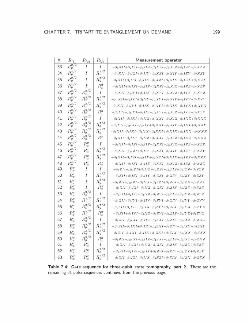
CHAPTER 7. TRIPARTITE ENTANGLEMENT ON DEMAND 199
# RQ1 RQ2 RQ3 Measurement operator33 R
π/2y I I −β1XII+β2IZI+β3IIZ−β4XZI−β5XIZ+β6IZZ−β7XZZ
34 Rπ/2y I R
π/2x −β1XII+β2IZI+β3IIY−β4XZI−β5XIY+β6IZY−β7XZY
35 Rπ/2y I R
π/2y −β1XII+β2IZI−β3IIX−β4XZI+β5XIX−β6IZX+β7XZX
36 Rπ/2y I Rπ
x −β1XII+β2IZI−β3IIZ−β4XZI+β5XIZ−β6IZZ+β7XZZ
37 Rπ/2y R
π/2x I −β1XII+β2IY I+β3IIZ−β4XY I−β5XIZ+β6IY Z−β7XY Z
38 Rπ/2y R
π/2x R
π/2x −β1XII+β2IY I+β3IIY−β4XY I−β5XIY+β6IY Y−β7XY Y
39 Rπ/2y R
π/2x R
π/2y −β1XII+β2IY I−β3IIX−β4XY I+β5XIX−β6IY X+β7XYX
40 Rπ/2y R
π/2x Rπ
x −β1XII+β2IY I−β3IIZ−β4XY I+β5XIZ−β6IY Z+β7XY Z
41 Rπ/2y R
π/2y I −β1XII−β2IXI+β3IIZ+β4XXI−β5XIZ−β6IXZ+β7XXZ
42 Rπ/2y R
π/2y R
π/2x −β1XII−β2IXI+β3IIY+β4XXI−β5XIY−β6IXY+β7XXY
43 Rπ/2y R
π/2y R
π/2y −β1XII−β2IXI−β3IIX+β4XXI+β5XIX+β6IXX−β7XXX
44 Rπ/2y R
π/2y Rπ
x −β1XII−β2IXI−β3IIZ+β4XXI+β5XIZ+β6IXZ−β7XXZ
45 Rπ/2y Rπ
x I −β1XII−β2IZI+β3IIZ+β4XZI−β5XIZ−β6IZZ+β7XZZ
46 Rπ/2y Rπ
x Rπ/2x −β1XII−β2IZI+β3IIY+β4XZI−β5XIY−β6IZY+β7XZY
47 Rπ/2y Rπ
x Rπ/2y −β1XII−β2IZI−β3IIX+β4XZI+β5XIX+β6IZX−β7XZX
48 Rπ/2y Rπ
x Rπx −β1XII−β2IZI−β3IIZ+β4XZI+β5XIZ+β6IZZ−β7XZZ
49 Rπx I I −β1ZII+β2IZI+β3IIZ−β4ZZI−β5ZIZ+β6IZZ−β7ZZZ
50 Rπx I R
π/2x −β1ZII+β2IZI+β3IIY−β4ZZI−β5ZIY+β6IZY−β7ZZY
51 Rπx I R
π/2y −β1ZII+β2IZI−β3IIX−β4ZZI+β5ZIX−β6IZX+β7ZZX
52 Rπx I Rπ
x −β1ZII+β2IZI−β3IIZ−β4ZZI+β5ZIZ−β6IZZ+β7ZZZ
53 Rπx R
π/2x I −β1ZII+β2IY I+β3IIZ−β4ZY I−β5ZIZ+β6IY Z−β7ZY Z
54 Rπx R
π/2x R
π/2x −β1ZII+β2IY I+β3IIY−β4ZY I−β5ZIY+β6IY Y−β7ZY Y
55 Rπx R
π/2x R
π/2y −β1ZII+β2IY I−β3IIX−β4ZY I+β5ZIX−β6IY X+β7ZY X
56 Rπx R
π/2x Rπ
x −β1ZII+β2IY I−β3IIZ−β4ZY I+β5ZIZ−β6IY Z+β7ZY Z
57 Rπx R
π/2y I −β1ZII−β2IXI+β3IIZ+β4ZXI−β5ZIZ−β6IXZ+β7ZXZ
58 Rπx R
π/2y R
π/2x −β1ZII−β2IXI+β3IIY+β4ZXI−β5ZIY−β6IXY+β7ZXY
59 Rπx R
π/2y R
π/2y −β1ZII−β2IXI−β3IIX+β4ZXI+β5ZIX+β6IXX−β7ZXX
60 Rπx R
π/2y Rπ
x −β1ZII−β2IXI−β3IIZ+β4ZXI+β5ZIZ+β6IXZ−β7ZXZ
61 Rπx Rπ
x I −β1ZII−β2IZI+β3IIZ+β4ZZI−β5ZIZ−β6IZZ+β7ZZZ
62 Rπx Rπ
x Rπ/2x −β1ZII−β2IZI+β3IIY+β4ZZI−β5ZIY−β6IZY+β7ZZY
63 Rπx Rπ
x Rπ/2y −β1ZII−β2IZI−β3IIX+β4ZZI+β5ZIX+β6IZX−β7ZZX
Table 7.4: Gate sequence for three-qubit state tomography, part 2. These are theremaining 31 pulse sequences continued from the previous page.
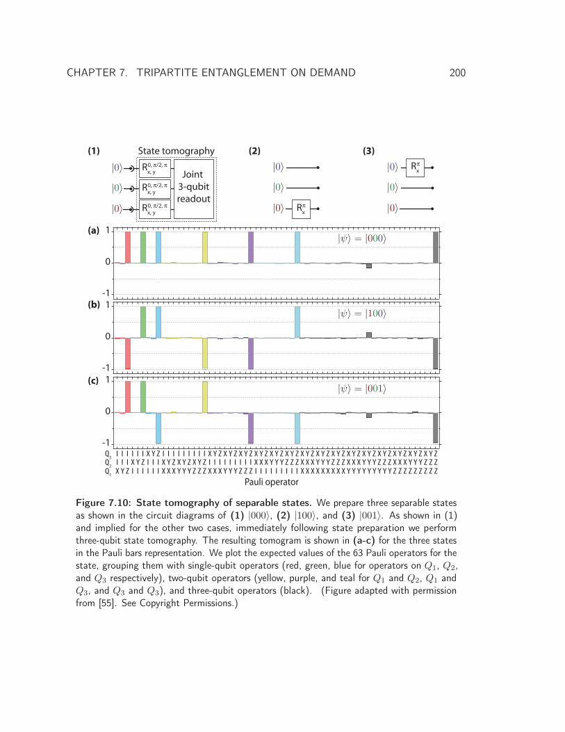
CHAPTER 7. TRIPARTITE ENTANGLEMENT ON DEMAND 200
State tomography
Joint 3-qubitreadout
(1)
|0〉|0〉|0〉
Rx, y0, /2,
Rx, y0, /2,
Rx, y0, /2,
|0〉|0〉|0〉 Rx
|0〉|0〉|0〉
Rx
(a)
(2)
(b)
(c)
(3)
IIX
IIY
IIZ
IXI
IYI
IZI
XII
YII
ZII
IXX
IYX
IZX
IXY
IYY
IZY
IXZ
IYZ
IZZI I I I I I I I I
I I I I I I I I IX X X Y Y Y Z Z Z
X Y Z X Y Z X Y Z X Y Z X Y Z X Y ZX X X Y Y Y Z Z Z
X Y Z X Y Z X Y Z X Y Z X Y Z X Y Z X Y Z X Y Z X Y ZX X X Y Y Y Z Z Z X X X Y Y Y Z Z Z X X X Y Y Y Z Z ZX X X X X X X X X Y Y Y Y Y Y Y Y Y Z Z Z Z Z Z Z Z Z
Pauli operatorQ1Q2Q3
|ψ〉 = |000〉
|ψ〉 = |100〉
|ψ〉 = |001〉
Figure 7.10: State tomography of separable states. We prepare three separable statesas shown in the circuit diagrams of (1) |000〉, (2) |100〉, and (3) |001〉. As shown in (1)and implied for the other two cases, immediately following state preparation we performthree-qubit state tomography. The resulting tomogram is shown in (a-c) for the three statesin the Pauli bars representation. We plot the expected values of the 63 Pauli operators for thestate, grouping them with single-qubit operators (red, green, blue for operators on Q1, Q2,and Q3 respectively), two-qubit operators (yellow, purple, and teal for Q1 and Q2, Q1 andQ3, and Q3 and Q3), and three-qubit operators (black). (Figure adapted with permissionfrom [55]. See Copyright Permissions.)
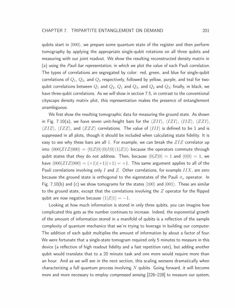
CHAPTER 7. TRIPARTITE ENTANGLEMENT ON DEMAND 201
qubits start in |000〉, we prepare some quantum state of the register and then performtomography by applying the appropriate single-qubit rotations on all three qubits andmeasuring with our joint readout. We show the resulting reconstructed density matrix in(a) using the Pauli bar representation, in which we plot the value of each Pauli correlation.The types of correlations are segregated by color: red, green, and blue for single-qubitcorrelations of Q1, Q2, and Q3 respectively, followed by yellow, purple, and teal for two-qubit correlations between Q1 and Q2, Q1 and Q3, and Q2 and Q3; finally, in black, wehave three-qubit correlations. As we will show in section 7.5, in contrast to the conventionalcityscape density matrix plot, this representation makes the presence of entanglementunambiguous.
We first show the resulting tomographic data for measuring the ground state. As shownin Fig. 7.10(a), we have seven unit-height bars for the 〈ZII〉, 〈IZI〉, 〈IIZ〉, 〈ZZI〉,〈ZIZ〉, 〈IZZ〉, and 〈ZZZ〉 correlations. The value of 〈III〉 is defined to be 1 and issuppressed in all plots, though it should be included when calculating state fidelity. It iseasy to see why these bars are all 1. For example, we can break the ZIZ correlator upinto 〈000|ZIZ|000〉 = 〈0|Z|0〉〈0|I|0〉〈1|Z|1〉 because the operators commute throughqubit states that they do not address. Then, because 〈0|Z|0〉 = 1 and 〈0|0〉 = 1, wehave 〈000|ZIZ|000〉 = (+1)(+1)(+1) = +1. This same argument applies to all of thePauli correlations involving only I and Z. Other correlations, for example IIX, are zerobecause the ground state is orthogonal to the eigenstates of the Pauli σx operator. InFig. 7.10(b) and (c) we show tomograms for the states |100〉 and |001〉. These are similarto the ground state, except that the correlations involving the Z operator for the flippedqubit are now negative because 〈1|Z|1〉 = −1.
Looking at how much information is stored in only three qubits, you can imagine howcomplicated this gets as the number continues to increase. Indeed, the exponential growthof the amount of information stored in a manifold of qubits is a reflection of the samplecomplexity of quantum mechanics that we’re trying to leverage in building our computer.The addition of each qubit multiplies the amount of information by about a factor of four.We were fortunate that a single-state tomogram required only 5 minutes to measure in thisdevice (a reflection of high readout fidelity and a fast repetition rate), but adding anotherqubit would translate that to a 20 minute task and one more would require more thanan hour. And as we will see in the next section, this scaling worsens dramatically whencharacterizing a full quantum process involving N qubits. Going forward, it will becomemore and more necessary to employ compressed sensing [226–228] to measure our system,
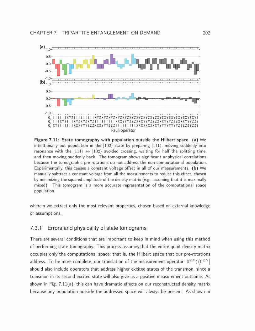
CHAPTER 7. TRIPARTITE ENTANGLEMENT ON DEMAND 202
(a)
(b)
IIX
IIY
IIZ
IXI
IYI
IZI
XII
YII
ZII
IXX
IYX
IZX
IXY
IYY
IZY
IXZ
IYZ
IZZI I I I I I I I I
I I I I I I I I IX X X Y Y Y Z Z Z
X Y Z X Y Z X Y Z X Y Z X Y Z X Y ZX X X Y Y Y Z Z Z
X Y Z X Y Z X Y Z X Y Z X Y Z X Y Z X Y Z X Y Z X Y ZX X X Y Y Y Z Z Z X X X Y Y Y Z Z Z X X X Y Y Y Z Z ZX X X X X X X X X Y Y Y Y Y Y Y Y Y Z Z Z Z Z Z Z Z Z
Pauli operatorQ1Q2Q3
Figure 7.11: State tomography with population outside the Hilbert space. (a) Weintentionally put population in the |102〉 state by preparing |111〉, moving suddenly intoresonance with the |111〉 ↔ |102〉 avoided crossing, waiting for half the splitting time,and then moving suddenly back. The tomogram shows significant unphysical correlationsbecause the tomographic pre-rotations do not address the non-computational population.Experimentally, this causes a constant voltage offset in all of our measurements. (b) Wemanually subtract a constant voltage from all the measurements to reduce this effect, chosenby minimizing the squared amplitude of the density matrix (e.g. assuming that it is maximallymixed). This tomogram is a more accurate representation of the computational spacepopulation.
wherein we extract only the most relevant properties, chosen based on external knowledgeor assumptions.
7.3.1 Errors and physicality of state tomograms
There are several conditions that are important to keep in mind when using this methodof performing state tomography. This process assumes that the entire qubit density matrixoccupies only the computational space; that is, the Hilbert space that our pre-rotationsaddress. To be more complete, our translation of the measurement operator
∣∣0⊗N⟩⟨0⊗N
∣∣should also include operators that address higher excited states of the transmon, since atransmon in its second excited state will also give us a positive measurement outcome. Asshown in Fig. 7.11(a), this can have dramatic effects on our reconstructed density matrixbecause any population outside the addressed space will always be present. As shown in
CHAPTER 7. TRIPARTITE ENTANGLEMENT ON DEMAND 203
Fig. 7.11(b), it will cause an offset voltage, as if our value for β0 is incorrect. (In Ref. 55,this was explicitly excised with the addition of a best-fit parameter to β0 that was chosento minimize the sum of the magnitude of the bars. This strategy was not used in Ref. 201.)We also assume that our β values are calibrated with perfectly prepared test states. Ifthere is some thermal equilibrium qubit population, for example, we will only address the“pure” quantum amplitude given by P (|0〉)− P (|1〉). Thus, the fidelities we claim fromtomography do not take into account the impurity of our ground state. Finally, if ourmeasurement pre-rotations are imperfect, our inferred values will also be flawed [169, 225].
All of these issues contribute to the un-physicality of our reconstructed density matrix.Our density matrix automatically has the required property tr (ρ) = 1 since 〈I⊗N〉 ≡ 1.However, a physical matrix must additionally have all positive eigenvalues, which is notguaranteed here. For example, nothing prevents the inferred value of a Pauli correlationfrom being larger than ±1, be it due to noise or systematic errors. This adds ambiguityto the definition of things like state fidelities, which involve taking a dot product of themeasured Pauli correlations with their ideal values. This is an especially large problemwhen fidelities approach 100%, since there is a significant difference in a state fidelity of99.9% and 99.0% from the point of view of fault tolerant error correction. Estimating thesize of both systematic and random errors presents a challenge.
There are several strategies to deal with these sources of error. You want your statetomograms to be as reliable as possible. This involves calibrating single-qubit rotations aswell as you can, both when addressing a single qubit and when simultaneously rotatingmultiple qubits. Running sequences like AllXY with and without auxiliary π pulses, asdescribed in section 5.2.3, can help, as can its more sensitive derivatives. In a recentpaper [169], it was also necessary to use NMR-inspired composite rotations that are lesssusceptible to certain types of errors.
It has become common to perform a maximum likelihood estimation of the densitymatrix [229, 230]. This process applies Lagrange multipliers to the inferred Pauli correlationvalues to enforce the physicality. As described in section 2.5.2 of Jerry Chow’s thesis[114], this involves evaluating polynomial functions of measurement results and is thereforenonlinear. This complicates the estimation of uncertainties. A maximum likelihoodestimation makes the smallest possible changes to the matrix to make it physical, whichis most justifiable when random errors are the dominant source of un-physicality [231].These changes are arbitrary, however. If we have systematic rather than random errors,there is no particular reason to trust the maximum-likelihood matrix more than the original
CHAPTER 7. TRIPARTITE ENTANGLEMENT ON DEMAND 204
one. Nevertheless, many research groups [216, 231, 232] use this process and argue thatwithout enforcing physicality, metrics like state fidelity have no meaning.
Finally, there has been a recent proposal to perform tomography in a self-consistent wayby oversampling the action of our measurement pre-rotations [225]. The idea is to relaxthe assumption that the unitary rotations we perform prior to measurement are perfect,and instead to infer their effect by extensively sampling measurement results following theirapplication. While this approach should mitigate one source of systematic error, it stillrequires nonlinear convex optimization. Though there exists a linear map of measurementresults to the process matrix of each of our rotations, measurements have finite noisewhich will be magnified in the state tomogram unless it is mitigated. In order to makethis optimization tractable, the authors linearize the involved equations. This has theeffect of simplifying the math, but also requires that the rotations used are fairly closeto the intended rotations around which the equations were expanded. Nevertheless, thismethod promises to reduce sensitivity to errors and enforce physicality in a more realisticand thoughtful way than a relatively crude maximum likelihood estimation.
7.4 Process tomography
What if we are interested not in the density matrix of a state, but rather, in the unitaryevolution of a process. For example, suppose someone gives us a black box which takes asan input N qubits and gives the same number as an output, but with a modified state.How can we determine the action of the box? To begin, we might insert the ground state(|00〉, supposing for now that N = 2) and measure the density matrix of the output state.We must perform many measurements to perform state tomography, so we prepare anensemble of our test ground states and apply the process to each. This will tell us onlya tiny amount about what the box does: we will learn its affect on the ground state.For two qubits, that accounts for only one point in 4-dimensional Hilbert space with 16orthogonal basis vectors. We send another state through, selecting this time the statein which the first qubit is pointing along the x-axis and the other is in its ground state((|00〉 + |10〉) /√2). This is actually a huge improvement over having only one pointbecause quantum mechanics is linear. Since we know the output density matrix for bothstates, we also know what happens to any superposition of those states: the result of anyrotation about the y-axis on the first qubit alone. If we know how the process affects eachof the 4N basis states for N qubits, in principle, we know everything about the process.
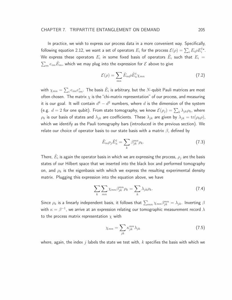
CHAPTER 7. TRIPARTITE ENTANGLEMENT ON DEMAND 205
In practice, we wish to express our process data in a more convenient way. Specifically,following equation 2.12, we want a set of operators Ei for the process E(ρ) =∑
i EiρE†i∗.
We express these operators Ei in some fixed basis of operators Ei such that Ei =∑m eimEm, which we may plug into the expression for E above to give
E(ρ) =∑mn
EmρE†nχmn (7.2)
with χmn =∑
i eime∗im. The basis Ei is arbitrary, but the N -qubit Pauli matrices are most
often chosen. The matrix χ is the “chi-matrix representation” of our process, and measuringit is our goal. It will contain d4 − d2 numbers, where d is the dimension of the system(e.g. d = 2 for one qubit). From state tomography, we know E(ρj) =
∑k λjkρk, where
ρk is our basis of states and λjk are coefficients. These λjk are given by λjk = tr(ρkρ),which we identify as the Pauli tomography bars (introduced in the previous section). Werelate our choice of operator basis to our state basis with a matrix β, defined by
EmρjE†n =
∑k
βmnjk ρk. (7.3)
There, Ei is again the operator basis in which we are expressing the process, ρj are the basisstates of our Hilbert space that we inserted into the black box and performed tomographyon, and ρk is the eigenbasis with which we express the resulting experimental densitymatrix. Plugging this expression into the equation above, we have∑
k
∑mn
χmnβmnjk ρk =
∑k
λjkρk. (7.4)
Since ρk is a linearly independent basis, it follows that∑
mn χmnβmnjk = λjk. Inverting β
with κ = β−1, we arrive at an expression relating our tomographic measurement record λ
to the process matrix representation χ with
χmn =∑jk
κmnjk λjk (7.5)
where, again, the index j labels the state we test with, k specifies the basis with which we
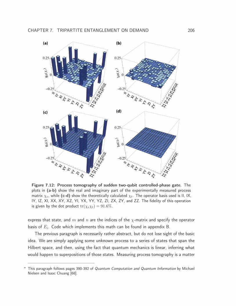
CHAPTER 7. TRIPARTITE ENTANGLEMENT ON DEMAND 206
Figure 7.12: Process tomography of sudden two-qubit controlled-phase gate. Theplots in (a-b) show the real and imaginary part of the experimentally measured processmatrix χe, while (c-d) show the theoretically calculated χt. The operator basis used is II, IX,IY, IZ, XI, XX, XY, XZ, YI, YX, YY, YZ, ZI, ZX, ZY, and ZZ. The fidelity of this operationis given by the dot product tr(χeχt) = 91.6%.
express that state, and m and n are the indices of the χ-matrix and specify the operatorbasis of Ei. Code which implements this math can be found in appendix B.
The previous paragraph is necessarily rather abstract, but do not lose sight of the basicidea. We are simply applying some unknown process to a series of states that span theHilbert space, and then, using the fact that quantum mechanics is linear, inferring whatwould happen to superpositions of those states. Measuring process tomography is a matter
∗ This paragraph follows pages 390-392 of Quantum Computation and Quantum Information by MichaelNielsen and Isaac Chuang [68].
CHAPTER 7. TRIPARTITE ENTANGLEMENT ON DEMAND 207
of measuring state tomography many times. In Fig. 7.12, we show the experimental andtheoretical process matrix for a sudden two-qubit controlled-phase gate. The matrix χ
can be complex-valued, depending on the operator basis used, and so we plot both thereal and imaginary parts. Just as with state tomography, process tomography can alsosuffer from unphysical errors. For this reason, significant effort has been made recently indeveloping more robust and efficient ways to characterize processes [188, 232–236].
7.5 Entanglement on demand
Now that we have the tools of entangling gates and efficient state tomography, we candemonstrate entanglement. We begin with the simple case of generating entanglementbetween only two qubits. The gate sequence for generating a Bell state between Q2 andQ3 is shown in Fig. 7.13(a). We start by putting both qubits in a superposition of |0〉and |1〉 with π/2 rotations about the y-axis of the Bloch sphere, with Q1 unused. Thistransfers |000〉 → |0〉 ⊗ (|00〉 + |10〉 + |01〉 + |11〉) /2. We then apply a cPhase gate (inthis case, we use the sudden version described above) with the −1 sign set to the |01〉state, giving us |ψ〉 = |0〉 ⊗ (|00〉 + |10〉 − |01〉 + |11〉) /2. At this point, we are in amaximally entangled Bell state of the top two qubits, though it is not yet in an easilyrecognizable configuration. To achieve that, we finish with a second π/2 rotation about yon Q3 to give us |Bell23〉 = |0〉 ⊗ (|00〉 + |11〉) /√2 – the canonical Bell state.
We perform state tomography on the result of this procedure, shown in Fig. 7.13(b).The order of the Pauli correlations emphasizes entanglement. As previously mentioned, thefirst three sets, denoted in red, green, and blue, show single-qubit correlations. Note thatwhile there is a strong (ideally, +1) Z correlation for Q1, there are no nonzero single-qubitcorrelations for either Q2 or Q3. This might be an indication that both of those qubitsare in a fully mixed state; however, looking further down the tomogram, we find thatwe have strong two-qubit correlations between these qubits (in IXX, IY Y , and IZZ).This is an unambiguous sign of entanglement between those two qubits: neither qubit hasany individual character, but considered simultaneously with its pair, we observe strongcorrelations. We also see that the two-qubit correlations involving Q1 and either Q2 orQ3 are zero, again reinforcing the idea that Q2 and Q3 cannot be described separately.Finally, we have three-qubit correlations which are a trivial extension of our two-qubitcorrelations plus Q1 in its ground state. The fidelity of this state to the intended state is
CHAPTER 7. TRIPARTITE ENTANGLEMENT ON DEMAND 208
(1)
|0〉|0〉|0〉
Ry/2
(a)
(b)
IIX
IIY
IIZ
IXI
IYI
IZI
XII
YII
ZII
IXX
IYX
IZX
IXY
IYY
IZY
IXZ
IYZ
IZZI I I I I I I I I
I I I I I I I I IX X X Y Y Y Z Z Z
X Y Z X Y Z X Y Z X Y Z X Y Z X Y ZX X X Y Y Y Z Z Z
X Y Z X Y Z X Y Z X Y Z X Y Z X Y Z X Y Z X Y Z X Y ZX X X Y Y Y Z Z Z X X X Y Y Y Z Z Z X X X Y Y Y Z Z ZX X X X X X X X X Y Y Y Y Y Y Y Y Y Z Z Z Z Z Z Z Z Z
Pauli operatorQ1Q2Q3
Ry/2
01Ry
/2(2)
|0〉|0〉|0〉
Ry/2
Ry/2
01Ry
/2
Ry/2
10Ry
/2
|ψ〉 = |0〉 ⊗ (|00〉 + |11〉) /√2
|ψ〉 = (|000〉 + |111〉) /√2
= 94%
= 88%
Figure 7.13: Circuit model and state tomography of Bell and GHZ states. In (1)we show the circuit for preparing a Bell state between Q2 and Q3. Lines between qubittracks terminating in circles indicates a controlled-phase gate, with the state receiving the −1sign indicated adjacent to the line. In (a) we show the Pauli bar tomogram of the resultingstate. Q1 still has a single-qubit Z correlation of +1 because it is in the ground state, butQ2 and Q3 have no single-qubit correlation since they are entangled. They do have strongtwo-qubit correlations, however, which are echoed in the three-qubit correlations. The fidelityof this state to its target, calculated by taking a dot product of the Pauli bar vector with theideal one (including the value of +1 for 〈III〉), is 94%. In (2) we show a circuit to extendthe entanglement to all three qubits, and plot the measured tomogram in (b). The lack ofsingle-qubit correlations and presence of strong two- and three-qubit correlations indicatesthat this is a three-qubit entangled GHZ state. The resulting state fidelity is 88%. (Figureadapted with permission from [55]. See Copyright Permissions.)

CHAPTER 7. TRIPARTITE ENTANGLEMENT ON DEMAND 209
94%, calculated by taking the dot product of the ideal state vector with the measuredvalues (including the III bar) and dividing by 8.
To entangle all three qubits, we can extend this procedure with an additional cPhasegate. As shown in Fig. 7.13(2), we first put all three qubits on the equator of their Blochsphere. The state at this point will be an equal superposition of all computational states,given by
|ψ〉 = (|000〉 + |100〉 + |010〉 + |001〉 + |110〉 + |101〉 + |011〉 + |111〉) /2√2.
Performing conditional phase gates between Q2 and Q3 with the conditional phase on01 flips the phase of |001〉 and |101〉 (since the state of Q1 is irrelevant for that gate),and the second conditional phase gate between Q1 and Q2 with the phase on 10 flips thephase of |100〉 and |101〉. The concatenation of these two gates will thus flip |001〉 and|100〉 only, since |101〉 is flipped twice, yielding
|ψ〉 = (|000〉 − |100〉 + |010〉 − |001〉 + |110〉 + |101〉 + |011〉 + |111〉) /2√2.
As in the two-qubit case, this state is already a maximally entangled three-qubit state,though in this basis it is difficult to see that. Thus, to finish, we apply π/2 rotationsabout y on Q1 and Q3, which give us the simple and unambiguously entangled state|GHZ〉 = (|000〉 + |111〉) /√2. Like the Bell state, this state also has a special name: athree-qubit Greenberger-Horne-Zeilinger or GHZ state [70] (section 2.1.6).
The presence of three-qubit entanglement is clear when looking at the measured statetomogram depicted in Fig. 7.13(d). Following the argument we made for the case ofthe two-qubit Bell state, we see here that there are no nonzero single-qubit correlations.There are, however, strong two-qubit ZZ correlations of any pair of qubits. This alonetells us that all three qubits are entangled with one another. Though they do not pointin any particular direction by themselves, when measured as a group they have a definitedirection. There are also nontrivial three-qubit correlations of XXX, Y Y X, Y XY , andXY Y , which, as we will see later, are sufficient to witness three-qubit entanglement. Thefidelity of this state to the state we intended to create is 88%.

CHAPTER 7. TRIPARTITE ENTANGLEMENT ON DEMAND 210
Figure 7.14: Calculated separable and entangled state tomograms. We calculate thedensity matrices of the states produced by the circuits shown in (a) and (b) and plot theircityscape density matrices in (c) and (d). The state shown in (c) is separable and the statein (d) is a maximally-entangled Bell state between qubits 1 and 3, but it is very difficult todistinguish them in this representation (here ρ is real). The Pauli representation of the samestates, shown in (e) and (f) unambiguously communicates that the first state is separableand the second entangled because the first has strong single-qubit correlations and fewtwo-qubit ones, while the second is the opposite. This demonstrates the advantage of thePauli representation.
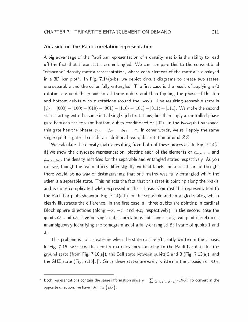
CHAPTER 7. TRIPARTITE ENTANGLEMENT ON DEMAND 211
An aside on the Pauli correlation representation
A big advantage of the Pauli bar representation of a density matrix is the ability to readoff the fact that these states are entangled. We can compare this to the conventional“cityscape” density matrix representation, where each element of the matrix is displayedin a 3D bar plot∗. In Fig. 7.14(a-b), we depict circuit diagrams to create two states,one separable and the other fully-entangled. The first case is the result of applying π/2
rotations around the y-axis to all three qubits and then flipping the phase of the topand bottom qubits with π rotations around the z-axis. The resulting separable state is|ψ〉 = |000〉− |100〉+ |010〉− |001〉− |110〉+ |101〉− |011〉+ |111〉. We make the secondstate starting with the same initial single-qubit rotations, but then apply a controlled-phasegate between the top and bottom qubits conditioned on |00〉. In the two-qubit subspace,this gate has the phases φ10 = φ01 = φ11 = π. In other words, we still apply the samesingle-qubit z gates, but add an additional two-qubit rotation around ZZ.
We calculate the density matrix resulting from both of these processes. In Fig. 7.14(c-d) we show the cityscape representation, plotting each of the elements of ρseparable andρentangled, the density matrices for the separable and entangled states respectively. As youcan see, though the two matrices differ slightly, without labels and a lot of careful thoughtthere would be no way of distinguishing that one matrix was fully entangled while theother is a separable state. This reflects the fact that this state is pointing along the x-axis,and is quite complicated when expressed in the z basis. Contrast this representation tothe Pauli bar plots shown in Fig. 7.14(e-f) for the separable and entangled states, whichclearly illustrates the difference. In the first case, all three qubits are pointing in cardinalBloch sphere directions (along +x, −x, and +x, respectively); in the second case thequbits Q1 and Q3 have no single-qubit correlations but have strong two-qubit correlations,unambiguously identifying the tomogram as of a fully-entangled Bell state of qubits 1 and3.
This problem is not as extreme when the state can be efficiently written in the z basis.In Fig. 7.15, we show the density matrices corresponding to the Pauli bar data for theground state (from Fig. 7.10[a]), the Bell state between qubits 2 and 3 (Fig. 7.13[a]), andthe GHZ state (Fig. 7.13[b]). Since these states are easily written in the z basis as |000〉,
∗ Both representations contain the same information since ρ =∑
O∈{III...ZZZ}〈O〉O. To convert in the
opposite direction, we have 〈0〉 = tr(ρO).

CHAPTER 7. TRIPARTITE ENTANGLEMENT ON DEMAND 212
0
1
-1
00.5
-0.5
00.5
-0.5
(a)
000
110
111
000001010011100101110
001010011100101111
Im( )Re( )
(b)
(c)
Figure 7.15: Cityscape density matrix representations of experimentally createdstates. These are the same states shown in the Pauli representation in Fig. 7.10(a) andFig. 7.13(a,b). Entangled states of two z eigenstates show the characteristic four corners ofa square pattern. These density matrices are simple because their states are easily written inthe z basis. (Figure used with permission from [55]. See Copyright Permissions.)
|0〉 ⊗ (|00〉 + |11〉) /√2, and (|000〉 + |111〉) /√2, the cityscape density matrices are notterribly complicated. Nevertheless, because this symmetry is not necessarily present for anygiven quantum state, we strongly favor the Pauli bar representation. This representationhas also been extended to more naturally express process matrices [54], though thatpractice has not yet been adopted by Schoelkopf lab.
Why entangle three qubits?
Why is three-qubit entanglement interesting? There are several reasons, but the primarilyone is the prospect of doing error correction. As we saw in section 2.3.4, the most basicquantum error correcting code requires three qubits. This code starts identically to theprocedure we have just demonstrated, encoding a quantum state in a three-qubit GHZstate. If we change the rotation axis of the π/2 rotation on Q2, we will create a different
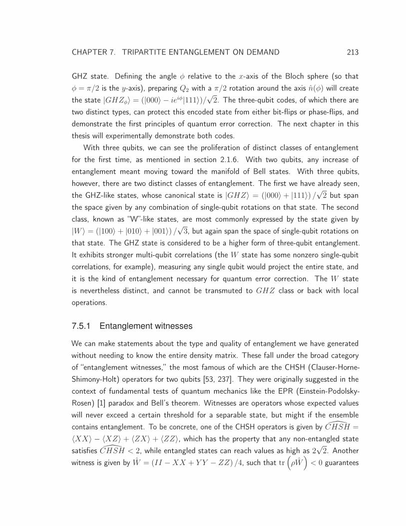
CHAPTER 7. TRIPARTITE ENTANGLEMENT ON DEMAND 213
GHZ state. Defining the angle φ relative to the x-axis of the Bloch sphere (so thatφ = π/2 is the y-axis), preparing Q2 with a π/2 rotation around the axis n(φ) will createthe state |GHZφ〉 = (|000〉 − ieiφ|111〉)/√2. The three-qubit codes, of which there aretwo distinct types, can protect this encoded state from either bit-flips or phase-flips, anddemonstrate the first principles of quantum error correction. The next chapter in thisthesis will experimentally demonstrate both codes.
With three qubits, we can see the proliferation of distinct classes of entanglementfor the first time, as mentioned in section 2.1.6. With two qubits, any increase ofentanglement meant moving toward the manifold of Bell states. With three qubits,however, there are two distinct classes of entanglement. The first we have already seen,the GHZ-like states, whose canonical state is |GHZ〉 = (|000〉 + |111〉) /√2 but spanthe space given by any combination of single-qubit rotations on that state. The secondclass, known as “W”-like states, are most commonly expressed by the state given by|W 〉 = (|100〉 + |010〉 + |001〉) /√3, but again span the space of single-qubit rotations onthat state. The GHZ state is considered to be a higher form of three-qubit entanglement.It exhibits stronger multi-qubit correlations (the W state has some nonzero single-qubitcorrelations, for example), measuring any single qubit would project the entire state, andit is the kind of entanglement necessary for quantum error correction. The W stateis nevertheless distinct, and cannot be transmuted to GHZ class or back with localoperations.
7.5.1 Entanglement witnesses
We can make statements about the type and quality of entanglement we have generatedwithout needing to know the entire density matrix. These fall under the broad categoryof “entanglement witnesses,” the most famous of which are the CHSH (Clauser-Horne-Shimony-Holt) operators for two qubits [53, 237]. They were originally suggested in thecontext of fundamental tests of quantum mechanics like the EPR (Einstein-Podolsky-Rosen) [1] paradox and Bell’s theorem. Witnesses are operators whose expected valueswill never exceed a certain threshold for a separable state, but might if the ensemblecontains entanglement. To be concrete, one of the CHSH operators is given by CHSH =
〈XX〉 − 〈XZ〉 + 〈ZX〉 + 〈ZZ〉, which has the property that any non-entangled statesatisfies CHSH < 2, while entangled states can reach values as high as 2
√2. Another
witness is given by W = (II − XX + Y Y − ZZ) /4, such that tr(ρW
)< 0 guarantees
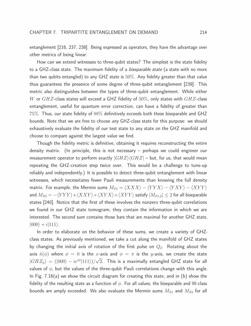
CHAPTER 7. TRIPARTITE ENTANGLEMENT ON DEMAND 214
entanglement [216, 237, 238]. Being expressed as operators, they have the advantage overother metrics of being linear.
How can we extend witnesses to three-qubit states? The simplest is the state fidelityto a GHZ-class state. The maximum fidelity of a biseparable state (a state with no morethan two qubits entangled) to any GHZ state is 50%. Any fidelity greater than that valuethus guarantees the presence of some degree of three-qubit entanglement [239]. Thismetric also distinguishes between the types of three-qubit entanglement. While eitherW or GHZ-class states will exceed a GHZ fidelity of 50%, only states with GHZ-classentanglement, useful for quantum error correction, can have a fidelity of greater than75%. Thus, our state fidelity of 88% definitively exceeds both these biseparable and GHZbounds. Note that we are free to choose any GHZ-class state for this purpose: we shouldexhaustively evaluate the fidelity of our test state to any state on the GHZ manifold andchoose to compare against the largest value we find.
Though the fidelity metric is definitive, obtaining it requires reconstructing the entiredensity matrix. (In principle, this is not necessary – perhaps we could engineer ourmeasurement operator to perform exactly |GHZ〉〈GHZ| – but, for us, that would meanrepeating the GHZ-creation step twice over. This would be a challenge to tune-upreliably and independently.) It is possible to detect three-qubit entanglement with linearwitnesses, which necessitates fewer Pauli measurements than knowing the full densitymatrix. For example, the Mermin sums MS1 = 〈XXX〉 − 〈Y Y X〉 − 〈Y XY 〉 − 〈XY Y 〉and MS2 = −〈Y Y Y 〉+〈XXY 〉+〈XYX〉+〈XY Y 〉 satisfy |MS1,2| ≤ 2 for all biseparablestates [240]. Notice that the first of these involves the nonzero three-qubit correlationswe found in our GHZ state tomogram; they contain the information in which we areinterested. The second sum contains those bars that are maximal for another GHZ state,|000〉 + i|111〉.
In order to elaborate on the behavior of these sums, we create a variety of GHZ-class states. As previously mentioned, we take a cut along the manifold of GHZ statesby changing the initial axis of rotation of the first pulse on Q2. Rotating about theaxis n(φ) where φ = 0 is the x-axis and φ = π is the y-axis, we create the state|GHZφ〉 = (|000〉 − ieiφ|111〉)/√2. This is a maximally entangled GHZ state for allvalues of φ, but the values of the three-qubit Pauli correlations change with this angle.In Fig. 7.16(a) we show the circuit diagram for creating this state, and in (b) show thefidelity of the resulting state as a function of φ. For all values, the biseparable and W-classbounds are amply exceeded. We also evaluate the Mermin sums MS1 and MS2 for all

CHAPTER 7. TRIPARTITE ENTANGLEMENT ON DEMAND 215
xy
z
n
(b)
quan
tum
clas
sica
l
Mer
min
sum
Fide
lity
(%)
100
75
50
-180 -90 0 90 180
4.0
2.0
0.0
4.0
2.0
Azimuthal angle (deg)
(c)
(a)
|0〉|0〉
|0〉Rn( )
/2
Ry/2
01Ry
/2
Ry/2
10Ry
/2
Repetition code|0〉
|1〉
MS1
MS2
Figure 7.16: Witnessing entanglement with fidelity and Mermin sum inequalities.(a) We map
(|0〉 − ieiφ|1〉) /√2 superpositions of Q2 into GHZ-class states |GHZφ〉 =(|000〉 − ieiφ|111〉) /√2 using the circuit shown. The indicated section constitutes theencoding step of the three-qubit quantum error correcting “repetition” code that will bediscussed in the following chapter. The fidelity of these states F = 〈GHZφ|ρ|GHZφ〉 as afunction of the azimuthal angle φ of the initial π/2 rotation of Q2 is plotted in (b) and hasan average value of 87%. This fidelity far exceeds biseparable and W-class bounds, witnessingstringent GHZ-class three-qubit entanglement. (c) Evolution of Mermin sums MS1 =〈XXX〉−〈Y Y X〉−〈Y XY 〉−〈XY Y 〉 and MS2 = −〈Y Y Y 〉+〈XXY 〉+〈XYX〉+〈XY Y 〉as a function of φ. Allowed values for quantum and biseparable states are labeled. For allvalues of φ, at least one of the sums exceeds the biseparable bound. For (b) and (c), thesolid lines result from a master equation simulation including only qubit decay during the81 ns pulse sequence. The fact that it predicts a similar fidelity to our experimental resultsuggests that pure dephasing and other errors are small contributions to infidelity. (Figureused with permission from [55]. See Copyright Permissions.)

CHAPTER 7. TRIPARTITE ENTANGLEMENT ON DEMAND 216
quan
tum
clas
sica
l
Mer
min
pro
duct
1.0
0.5
0.0
-1.0
-0.5
-180 -90 0 90 180Azimuthal angle (deg)
MP1 MP2
Figure 7.17: Witnessing three-qubit entanglement with Mermin product inequalities.The values of the Mermin products MP1 = 〈XXX〉〈Y Y X〉〈Y XY 〉〈XY Y 〉 and MP2 =〈Y Y Y 〉〈XXY 〉〈XYX〉〈Y XX〉 are plotted as a function of the angle φ of the preparedstate |GHZφ〉 =
(|000〉 − ieiφ|111〉) /√2. The most negative value measured, −0.52±0.05,violates the biseparable and LHV bound of −1/16 by 830±80%. The solid lines are the resultof a master equation simulation that includes qubit relaxation during the pulse sequence.(Figure used with permission from [55]. See Copyright Permissions.)
angles, shown in (c), and exceed the biseparable bound of at least one of the sums for allφ. It should be clear that although we defined only two Mermin sums, it is possible tocreate a MSφ, which is maximally violated for each value of φ. |MS1,2| ≤ 2 also defines alocal-hidden-variable (LHV) bound in the same way as the Bell test, which our extremalvalue of 3.4 ± 0.1 violates by 14 standard deviations [241]. However, we cannot refutelocal realism because we are not free of detection loopholes [242].
Figure 7.16(c) clearly demonstrates one downside of the Mermin sums: for most ofits allowed range of values, a sum will not distinguish between classical behavior andquantum behavior. Formally, this indicates that for three qubits, the biseparable rangesignificantly overlaps with the quantum range. We can compress this overlap by usinga nonlinear metric, amplifying three-qubit correlations that are due to entanglement.We define the Mermin products MP1 = 〈XXX〉〈Y Y X〉〈Y XY 〉〈XY Y 〉 and MP2 =
〈Y Y Y 〉〈XXY 〉〈XYX〉〈Y XX〉, which are a function of the same correlations as theMermin sums. For these metrics, we found through numerical exploration that biseparablestates obey −1/16 ≤ MP1,2 ≤ 1/64, which is small compared to the range spanned bythree-qubit quantum states, −1 ≤ MP1,2 ≤ 1/16 [55]. The LHV range for the Mermin
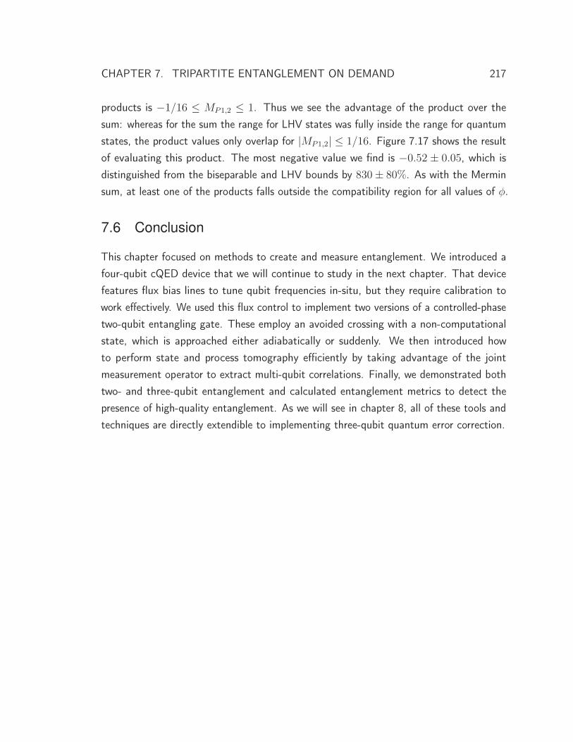
CHAPTER 7. TRIPARTITE ENTANGLEMENT ON DEMAND 217
products is −1/16 ≤ MP1,2 ≤ 1. Thus we see the advantage of the product over thesum: whereas for the sum the range for LHV states was fully inside the range for quantumstates, the product values only overlap for |MP1,2| ≤ 1/16. Figure 7.17 shows the resultof evaluating this product. The most negative value we find is −0.52 ± 0.05, which isdistinguished from the biseparable and LHV bounds by 830 ± 80%. As with the Merminsum, at least one of the products falls outside the compatibility region for all values of φ.
7.6 Conclusion
This chapter focused on methods to create and measure entanglement. We introduced afour-qubit cQED device that we will continue to study in the next chapter. That devicefeatures flux bias lines to tune qubit frequencies in-situ, but they require calibration towork effectively. We used this flux control to implement two versions of a controlled-phasetwo-qubit entangling gate. These employ an avoided crossing with a non-computationalstate, which is approached either adiabatically or suddenly. We then introduced howto perform state and process tomography efficiently by taking advantage of the jointmeasurement operator to extract multi-qubit correlations. Finally, we demonstrated bothtwo- and three-qubit entanglement and calculated entanglement metrics to detect thepresence of high-quality entanglement. As we will see in chapter 8, all of these tools andtechniques are directly extendible to implementing three-qubit quantum error correction.


CHAPTER 8
Quantum Error Correction with cQED
This chapter explains how we have implemented the most basic form of quantum errorcorrection in a cQED device. Though this demonstration has been done before in NMR
[243–246] and trapped ions [30, 247], this was the first realization in the solid state. Weperform the quantum repetition code that was introduced in section 2.3.4, implementingthe measurement-free version because we do not yet have the ability to individually measureand feed-forward ancilla states. As we saw, the key to this code is the three-qubit ccNOTor Toffoli gate, which coherently reverses an error on the primary qubit after decoding.Though this gate can be constructed with four of our existing cPhase gates, we insteadimplement a faster version using the higher level structure of the transmon qubits. Ourgate uses both adiabatic and sudden interactions, leveraging our understanding of the twocPhase gates that we have discussed previously. In the first half of this chapter, we willdetail how our gate works and is tuned up before verifying its action with both state andprocess tomography.
We combine this gate with our ability to create GHZ-like states to implement quantumerror correction in the second half of the chapter. After encoding an arbitrary quantumstate into the three-qubit manifold using the GHZ circuit, we apply intentional bit-rotationerrors to one of the qubits. We then reverse the encoding step, correct the errors with theToffoli gate, and perform state tomography on the output to verify our success. We also
219

CHAPTER 8. QUANTUM ERROR CORRECTION WITH CQED 220
demonstrate phase-flip error correction, which only requires a small change to the bit-flipcode. To more realistically evaluate its performance, we apply errors on all three qubitssimultaneously with some effective probability. The signature of success is a quadraticdependence of the fidelity of the final quantum state on this error probability, whichunambiguously verifies that errors are being corrected as expected.
8.1 Toffoli gate
As shown in section 2.3.4, the key ingredient to the autonomous three-qubit QEC code isthe Toffoli gate which implements the correction. This operation, which is also knownas the controlled-controlled-NOT or ccNOT gate, acts on a manifold of three qubitssimultaneously and is therefore a three-qubit gate. In addition to QEC, this gate isimportant for a variety of applications such as Shor’s factoring algorithm [14]. For thatreason, it has attracted significant experimental interest with recent implementations inlinear optics [248], trapped ions [249], and superconducting circuits [232, 250]. Thoughwe have not yet encountered such a gate in this thesis, since the combination of thecPhase gate and single-qubit rotations is universal, we know that we can directly constructa Toffoli gate from techniques already established. One possible construction is shownin Fig. 8.1, comprised of six cNOTs. (We could equivalently use cPhase gates here, withappropriate changes to the single-qubit rotations.) We can optimize this gate for thepurpose of autonomous error correction by taking advantage of the fact that the codecalls for two of the qubits to be measured or reset at the end of the operation. Thus, anyspurious entanglement between the ancillas is harmless and need not be corrected. Thisfreedom enables us to make a smaller construction using only four cNOTs, also in Fig. 8.1by omitting the red gates (which involve only the top two ancilla qubits) and swappingthe bottom corner of the resulting unitary matrix with diag{−i, i}.
Even this optimized pseudo-Toffoli takes quite a long time, however. If we assume thecPhase gates take 18 ns and the single-qubit rotations 12 ns (including 2 ns of paddingfor each), it requires at least 130 ns. This is quite intimidating, given that the coherencetimes for these qubits were less than 1 μs and including the cost of making and unmakinga GHZ state to perform the error correction code. Can we do better? While it has beenproven that a six-gate Toffoli is the shortest possible construction using cNOT gates [251],that fortunately only applies to two-level qubits. We can potentially use the higher levelstructure of the transmon qubits to engineer a more efficient gate.
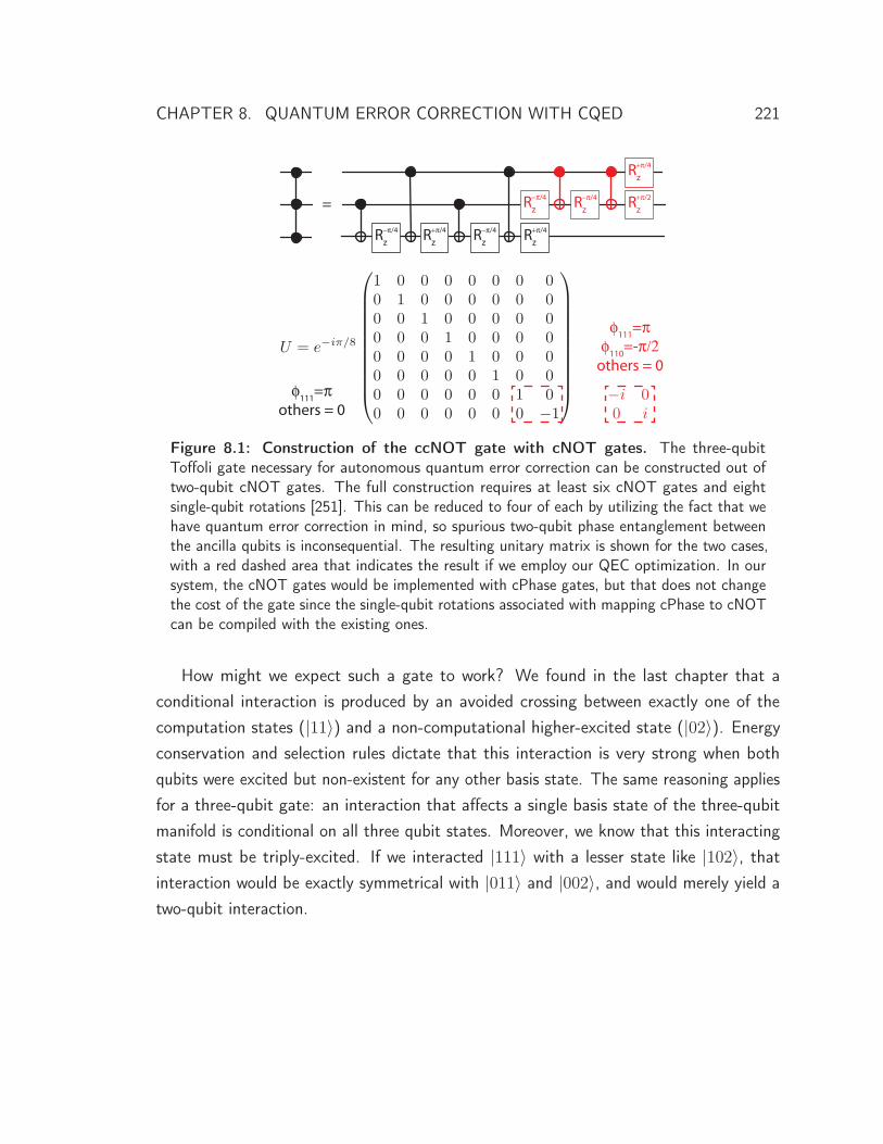
CHAPTER 8. QUANTUM ERROR CORRECTION WITH CQED 221
Rz/4 Rz
/4 Rz/4 Rz
/4
Rz/4 Rz
/4
Rz/4
Rz/2=
U = e−iπ/8
⎛⎜⎜⎜⎜⎜⎜⎜⎜⎜⎜⎝
1 0 0 0 0 0 0 00 1 0 0 0 0 0 00 0 1 0 0 0 0 00 0 0 1 0 0 0 00 0 0 0 1 0 0 00 0 0 0 0 1 0 00 0 0 0 0 0 1 00 0 0 0 0 0 0 −1
⎞⎟⎟⎟⎟⎟⎟⎟⎟⎟⎟⎠ −i 00 i
111=others = 0
111=
110=-others = 0
Figure 8.1: Construction of the ccNOT gate with cNOT gates. The three-qubitToffoli gate necessary for autonomous quantum error correction can be constructed out oftwo-qubit cNOT gates. The full construction requires at least six cNOT gates and eightsingle-qubit rotations [251]. This can be reduced to four of each by utilizing the fact that wehave quantum error correction in mind, so spurious two-qubit phase entanglement betweenthe ancilla qubits is inconsequential. The resulting unitary matrix is shown for the two cases,with a red dashed area that indicates the result if we employ our QEC optimization. In oursystem, the cNOT gates would be implemented with cPhase gates, but that does not changethe cost of the gate since the single-qubit rotations associated with mapping cPhase to cNOTcan be compiled with the existing ones.
How might we expect such a gate to work? We found in the last chapter that aconditional interaction is produced by an avoided crossing between exactly one of thecomputation states (|11〉) and a non-computational higher-excited state (|02〉). Energyconservation and selection rules dictate that this interaction is very strong when bothqubits were excited but non-existent for any other basis state. The same reasoning appliesfor a three-qubit gate: an interaction that affects a single basis state of the three-qubitmanifold is conditional on all three qubit states. Moreover, we know that this interactingstate must be triply-excited. If we interacted |111〉 with a lesser state like |102〉, thatinteraction would be exactly symmetrical with |011〉 and |002〉, and would merely yield atwo-qubit interaction.

CHAPTER 8. QUANTUM ERROR CORRECTION WITH CQED 222
8.1.1 Efficient Toffoli using higher levels
Here we will show how we used exactly that interaction of |111〉 with |003〉 to buildan efficient Toffoli-sign gate. This gate, also known as the controlled-controlled-Phaseor ccPhase, is related to the Toffoli by single-qubit rotations, just as the cPhase is tothe cNOT. We must discuss two major complications in getting it to work. The firstcomplication is that the direct interaction of these two states is extremely weak. There isno coupling of |111〉 to any state that changes its excitation by more than one to first order(e.g. there are strong interactions with states like |201〉 but not with |300〉). Higher-orderterms do enable some coupling, but will be less than 1 MHz and too slow to be useful. Insection 8.1.3, we will see the signature of this interaction and will verify that it is indeedtiny. To avoid this, we begin by swapping the quantum amplitude of the state |111〉 into|102〉, and, because the state of Q1 is irrelevant, |011〉 to |002〉. The |102〉 state hasa large avoided crossing with |003〉 that we use to generate our three-qubit conditionalphase. We then reverse the swap to transfer back to the computational space.
The second complication is that a three-qubit phase gate has seven independentparameters, four of which are due to nontrivial multi-qubit interactions. We can seethis by generalizing the notation that we introduced for the case of a two-qubit phasegate. We distinguish between types of phases, again mapping singly-excited states like|100〉 to eiφ100 |100〉 and doubly-excited states like |110〉 to ei(φ100+φ010+φ110)|110〉, thelatter of which has the conditional phase φ110, as seen with two-qubit gates. Onedifference here, however, is that there are three independent two-qubit phases betweeneach pair of qubits (φ110, φ101, and φ011), so |101〉 maps to ei(φ100+φ001+φ101)|101〉, witha phase linearly independent from the others. Finally, there is also a three-qubit phaseφ111 that is conditional on all three qubits being excited, so that the state |111〉 mapsto ei(φ100+φ010+φ001+φ110+φ101+φ011+φ111)|111〉. We can summarize this by saying that any
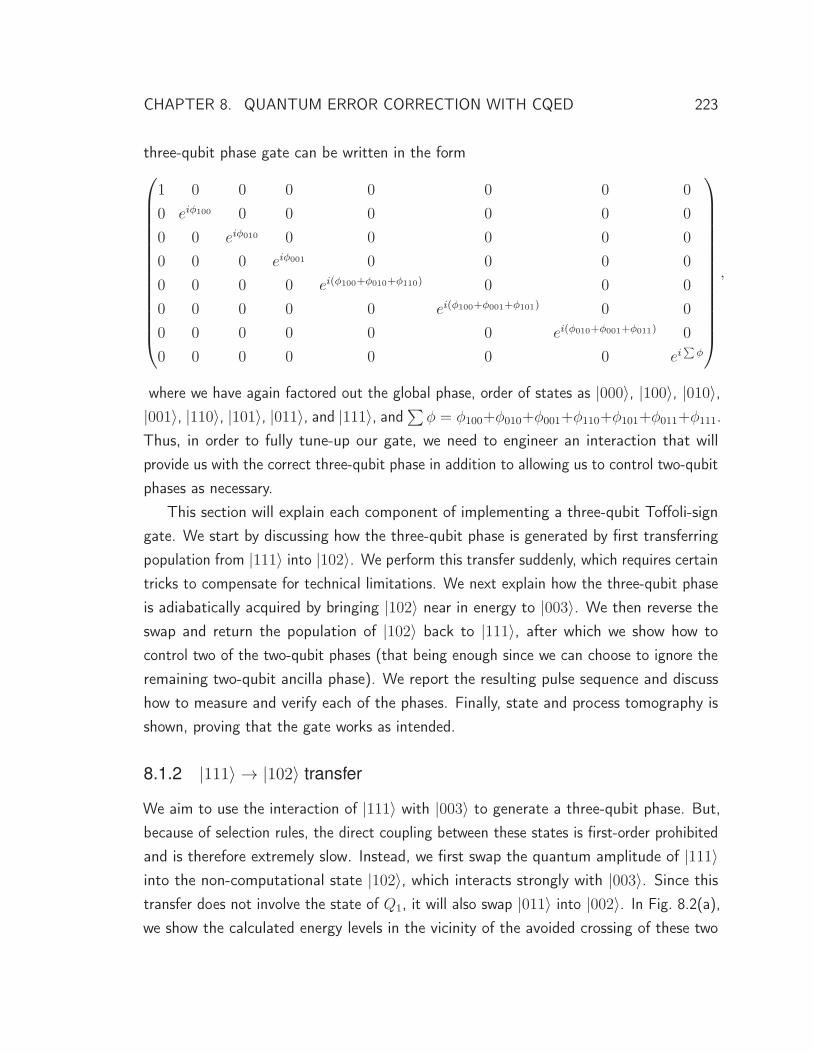
CHAPTER 8. QUANTUM ERROR CORRECTION WITH CQED 223
three-qubit phase gate can be written in the form⎛⎜⎜⎜⎜⎜⎜⎜⎜⎜⎜⎜⎜⎜⎜⎝
1 0 0 0 0 0 0 0
0 eiφ100 0 0 0 0 0 0
0 0 eiφ010 0 0 0 0 0
0 0 0 eiφ001 0 0 0 0
0 0 0 0 ei(φ100+φ010+φ110) 0 0 0
0 0 0 0 0 ei(φ100+φ001+φ101) 0 0
0 0 0 0 0 0 ei(φ010+φ001+φ011) 0
0 0 0 0 0 0 0 ei∑
φ
⎞⎟⎟⎟⎟⎟⎟⎟⎟⎟⎟⎟⎟⎟⎟⎠,
where we have again factored out the global phase, order of states as |000〉, |100〉, |010〉,|001〉, |110〉, |101〉, |011〉, and |111〉, and
∑φ = φ100+φ010+φ001+φ110+φ101+φ011+φ111.
Thus, in order to fully tune-up our gate, we need to engineer an interaction that willprovide us with the correct three-qubit phase in addition to allowing us to control two-qubitphases as necessary.
This section will explain each component of implementing a three-qubit Toffoli-signgate. We start by discussing how the three-qubit phase is generated by first transferringpopulation from |111〉 into |102〉. We perform this transfer suddenly, which requires certaintricks to compensate for technical limitations. We next explain how the three-qubit phaseis adiabatically acquired by bringing |102〉 near in energy to |003〉. We then reverse theswap and return the population of |102〉 back to |111〉, after which we show how tocontrol two of the two-qubit phases (that being enough since we can choose to ignore theremaining two-qubit ancilla phase). We report the resulting pulse sequence and discusshow to measure and verify each of the phases. Finally, state and process tomography isshown, proving that the gate works as intended.
8.1.2 |111〉 → |102〉 transfer
We aim to use the interaction of |111〉 with |003〉 to generate a three-qubit phase. But,because of selection rules, the direct coupling between these states is first-order prohibitedand is therefore extremely slow. Instead, we first swap the quantum amplitude of |111〉into the non-computational state |102〉, which interacts strongly with |003〉. Since thistransfer does not involve the state of Q1, it will also swap |011〉 into |002〉. In Fig. 8.2(a),we show the calculated energy levels in the vicinity of the avoided crossing of these two
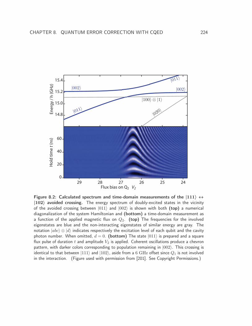
CHAPTER 8. QUANTUM ERROR CORRECTION WITH CQED 224
|100〉 ⊗ |1〉
|020〉|011〉
|002〉 |002〉|011〉
Figure 8.2: Calculated spectrum and time-domain measurements of the |111〉 ↔|102〉 avoided crossing. The energy spectrum of doubly-excited states in the vicinityof the avoided crossing between |011〉 and |002〉 is shown with both (top) a numericaldiagonalization of the system Hamiltonian and (bottom) a time-domain measurement asa function of the applied magnetic flux on Q2. (top) The frequencies for the involvedeigenstates are blue and the non-interacting eigenstates of similar energy are gray. Thenotation |abc〉 ⊗ |d〉 indicates respectively the excitation level of each qubit and the cavityphoton number. When omitted, d = 0. (bottom) The state |011〉 is prepared and a squareflux pulse of duration t and amplitude V2 is applied. Coherent oscillations produce a chevronpattern, with darker colors corresponding to population remaining in |002〉. This crossing isidentical to that between |111〉 and |102〉, aside from a 6 GHz offset since Q1 is not involvedin the interaction. (Figure used with permission from [201]. See Copyright Permissions.)
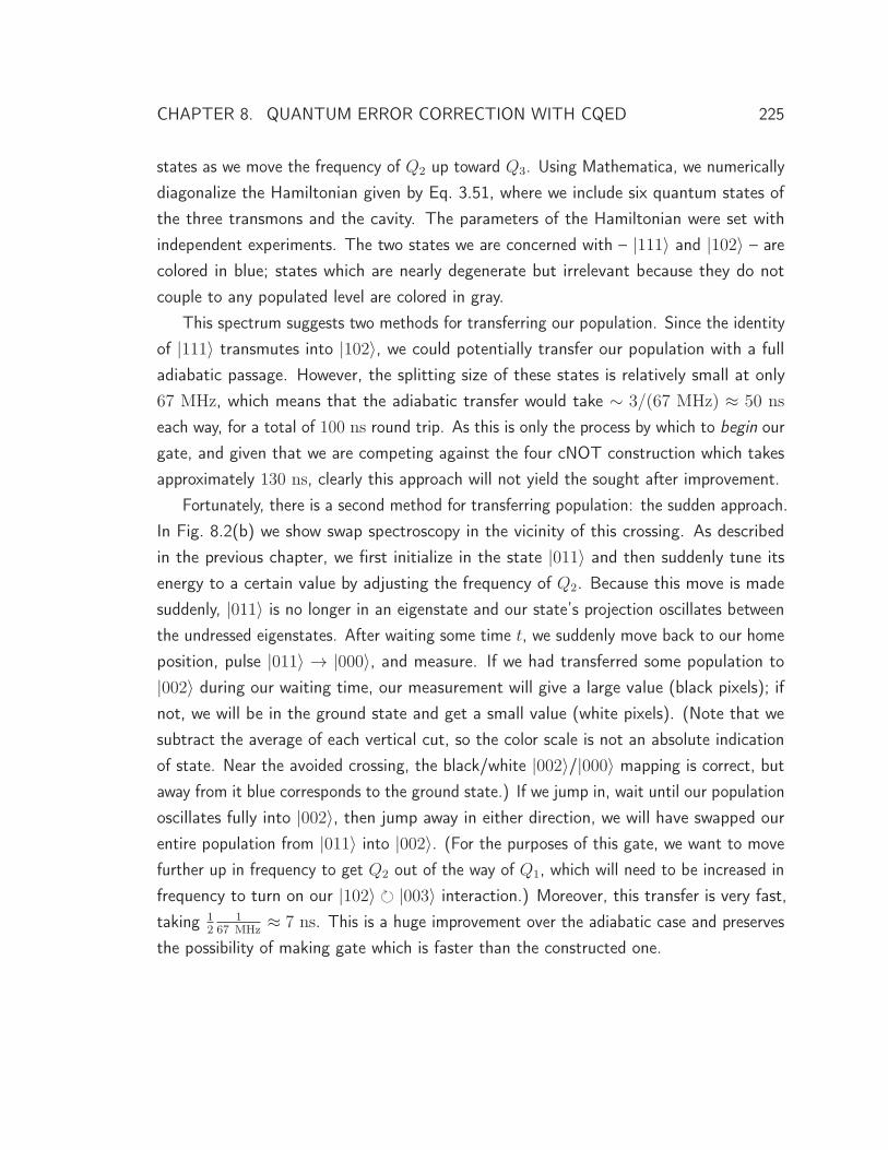
CHAPTER 8. QUANTUM ERROR CORRECTION WITH CQED 225
states as we move the frequency of Q2 up toward Q3. Using Mathematica, we numericallydiagonalize the Hamiltonian given by Eq. 3.51, where we include six quantum states ofthe three transmons and the cavity. The parameters of the Hamiltonian were set withindependent experiments. The two states we are concerned with – |111〉 and |102〉 – arecolored in blue; states which are nearly degenerate but irrelevant because they do notcouple to any populated level are colored in gray.
This spectrum suggests two methods for transferring our population. Since the identityof |111〉 transmutes into |102〉, we could potentially transfer our population with a fulladiabatic passage. However, the splitting size of these states is relatively small at only67 MHz, which means that the adiabatic transfer would take ∼ 3/(67 MHz) ≈ 50 ns
each way, for a total of 100 ns round trip. As this is only the process by which to begin ourgate, and given that we are competing against the four cNOT construction which takesapproximately 130 ns, clearly this approach will not yield the sought after improvement.
Fortunately, there is a second method for transferring population: the sudden approach.In Fig. 8.2(b) we show swap spectroscopy in the vicinity of this crossing. As describedin the previous chapter, we first initialize in the state |011〉 and then suddenly tune itsenergy to a certain value by adjusting the frequency of Q2. Because this move is madesuddenly, |011〉 is no longer in an eigenstate and our state’s projection oscillates betweenthe undressed eigenstates. After waiting some time t, we suddenly move back to our homeposition, pulse |011〉 → |000〉, and measure. If we had transferred some population to|002〉 during our waiting time, our measurement will give a large value (black pixels); ifnot, we will be in the ground state and get a small value (white pixels). (Note that wesubtract the average of each vertical cut, so the color scale is not an absolute indicationof state. Near the avoided crossing, the black/white |002〉/|000〉 mapping is correct, butaway from it blue corresponds to the ground state.) If we jump in, wait until our populationoscillates fully into |002〉, then jump away in either direction, we will have swapped ourentire population from |011〉 into |002〉. (For the purposes of this gate, we want to movefurther up in frequency to get Q2 out of the way of Q1, which will need to be increased infrequency to turn on our |102〉 � |003〉 interaction.) Moreover, this transfer is very fast,taking 1
21
67 MHz≈ 7 ns. This is a huge improvement over the adiabatic case and preserves
the possibility of making gate which is faster than the constructed one.
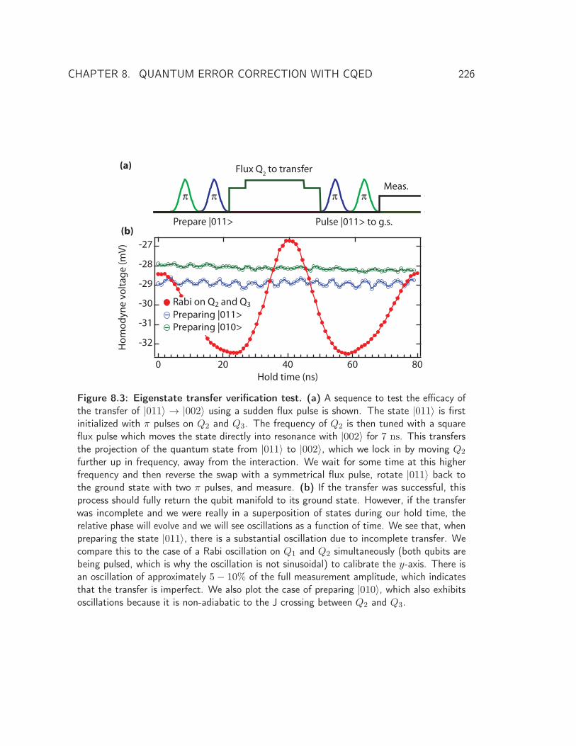
CHAPTER 8. QUANTUM ERROR CORRECTION WITH CQED 226
Prepare |011>
Flux Q2 to transfer
Pulse |011> to g.s.
Meas.
(a)
(b)
Figure 8.3: Eigenstate transfer verification test. (a) A sequence to test the efficacy ofthe transfer of |011〉 → |002〉 using a sudden flux pulse is shown. The state |011〉 is firstinitialized with π pulses on Q2 and Q3. The frequency of Q2 is then tuned with a squareflux pulse which moves the state directly into resonance with |002〉 for 7 ns. This transfersthe projection of the quantum state from |011〉 to |002〉, which we lock in by moving Q2
further up in frequency, away from the interaction. We wait for some time at this higherfrequency and then reverse the swap with a symmetrical flux pulse, rotate |011〉 back tothe ground state with two π pulses, and measure. (b) If the transfer was successful, thisprocess should fully return the qubit manifold to its ground state. However, if the transferwas incomplete and we were really in a superposition of states during our hold time, therelative phase will evolve and we will see oscillations as a function of time. We see that, whenpreparing the state |011〉, there is a substantial oscillation due to incomplete transfer. Wecompare this to the case of a Rabi oscillation on Q1 and Q2 simultaneously (both qubits arebeing pulsed, which is why the oscillation is not sinusoidal) to calibrate the y-axis. There isan oscillation of approximately 5 − 10% of the full measurement amplitude, which indicatesthat the transfer is imperfect. We also plot the case of preparing |010〉, which also exhibitsoscillations because it is non-adiabatic to the J crossing between Q2 and Q3.
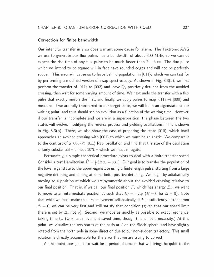
CHAPTER 8. QUANTUM ERROR CORRECTION WITH CQED 227
Correction for finite bandwidth
Our intent to transfer in 7 ns does warrant some cause for alarm. The Tektronix AWGwe use to generate our flux pulses has a bandwidth of about 300 MHz, so we cannotexpect the rise time of any flux pulse to be much faster than 2 − 3 ns. The flux pulsewhich we intend to be square will in fact have rounded edges and will not be perfectlysudden. This error will cause us to leave behind population in |011〉, which we can test forby performing a modified version of swap spectroscopy. As shown in Fig. 8.3(a), we firstperform the transfer of |011〉 to |002〉 and leave Q2 positively detuned from the avoidedcrossing, then wait for some varying amount of time. We next undo the transfer with a fluxpulse that exactly mirrors the first, and finally, we apply pulses to map |011〉 → |000〉 andmeasure. If we are fully transferred to our target state, we will be in an eigenstate at ourwaiting point, and thus should see no evolution as a function of the waiting time. However,if our transfer is incomplete and we are in a superposition, the phase between the twostates will evolve, modifying the reverse process and yielding oscillations. This is shownin Fig. 8.3(b). There, we also show the case of preparing the state |010〉, which itselfapproaches an avoided crossing with |001〉 to which we must be adiabatic. We compare itto the contrast of a |000〉 � |011〉 Rabi oscillation and find that the size of the oscillationis fairly substantial – almost 10% – which we must mitigate.
Fortunately, a simple theoretical procedure exists to deal with a finite transfer speed.Consider a test Hamiltonian H = 1
2(Δσz + gσx). Our goal is to transfer the population of
the lower eigenstate to the upper eigenstate using a finite-length pulse, starting from a largenegative detuning and ending at some finite positive detuning. We begin by adiabaticallymoving to a position at which we are symmetric about the avoided crossing relative toour final position. That is, if we call our final position F , which has energy EF , we wantto move to an intermediate position I, such that EI = −EF (E = 0 for Δ = 0). Notethat while we must make this first movement adiabatically, if F is sufficiently distant fromΔ = 0, we can be very fast and still satisfy that condition (given that our speed limitthere is set by Δ, not g). Second, we move as quickly as possible to exact resonance,taking time ts. (Our fast movement saved time, though this is not a necessity.) At thispoint, we visualize the two states of the basis at I on the Bloch sphere, and have slightlyrotated from the north pole in some direction due to our non-sudden trajectory. This smallrotation is directly accountable for the error that we are trying to correct.
At this point, our goal is to wait for a period of time τ that will bring the qubit to the
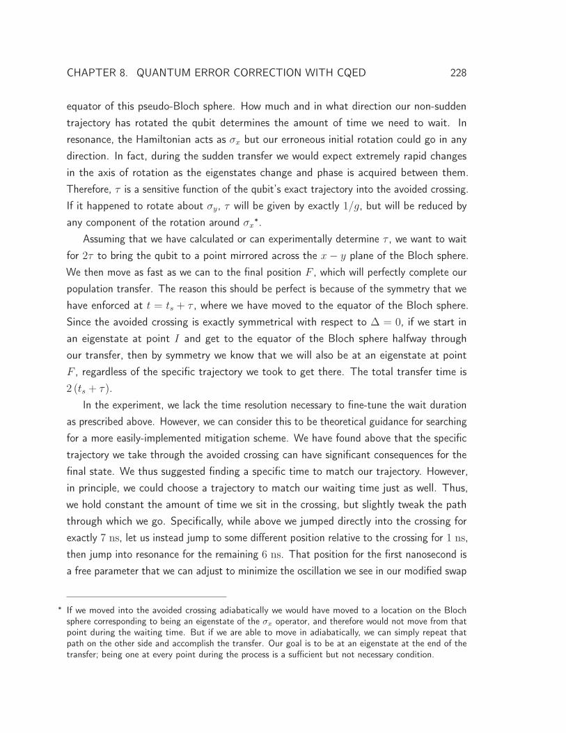
CHAPTER 8. QUANTUM ERROR CORRECTION WITH CQED 228
equator of this pseudo-Bloch sphere. How much and in what direction our non-suddentrajectory has rotated the qubit determines the amount of time we need to wait. Inresonance, the Hamiltonian acts as σx but our erroneous initial rotation could go in anydirection. In fact, during the sudden transfer we would expect extremely rapid changesin the axis of rotation as the eigenstates change and phase is acquired between them.Therefore, τ is a sensitive function of the qubit’s exact trajectory into the avoided crossing.If it happened to rotate about σy, τ will be given by exactly 1/g, but will be reduced byany component of the rotation around σx
∗.Assuming that we have calculated or can experimentally determine τ , we want to wait
for 2τ to bring the qubit to a point mirrored across the x − y plane of the Bloch sphere.We then move as fast as we can to the final position F , which will perfectly complete ourpopulation transfer. The reason this should be perfect is because of the symmetry that wehave enforced at t = ts + τ , where we have moved to the equator of the Bloch sphere.Since the avoided crossing is exactly symmetrical with respect to Δ = 0, if we start inan eigenstate at point I and get to the equator of the Bloch sphere halfway throughour transfer, then by symmetry we know that we will also be at an eigenstate at pointF , regardless of the specific trajectory we took to get there. The total transfer time is2 (ts + τ).
In the experiment, we lack the time resolution necessary to fine-tune the wait durationas prescribed above. However, we can consider this to be theoretical guidance for searchingfor a more easily-implemented mitigation scheme. We have found above that the specifictrajectory we take through the avoided crossing can have significant consequences for thefinal state. We thus suggested finding a specific time to match our trajectory. However,in principle, we could choose a trajectory to match our waiting time just as well. Thus,we hold constant the amount of time we sit in the crossing, but slightly tweak the paththrough which we go. Specifically, while above we jumped directly into the crossing forexactly 7 ns, let us instead jump to some different position relative to the crossing for 1 ns,then jump into resonance for the remaining 6 ns. That position for the first nanosecond isa free parameter that we can adjust to minimize the oscillation we see in our modified swap
∗ If we moved into the avoided crossing adiabatically we would have moved to a location on the Blochsphere corresponding to being an eigenstate of the σx operator, and therefore would not move from thatpoint during the waiting time. But if we are able to move in adiabatically, we can simply repeat thatpath on the other side and accomplish the transfer. Our goal is to be at an eigenstate at the end of thetransfer; being one at every point during the process is a sufficient but not necessary condition.
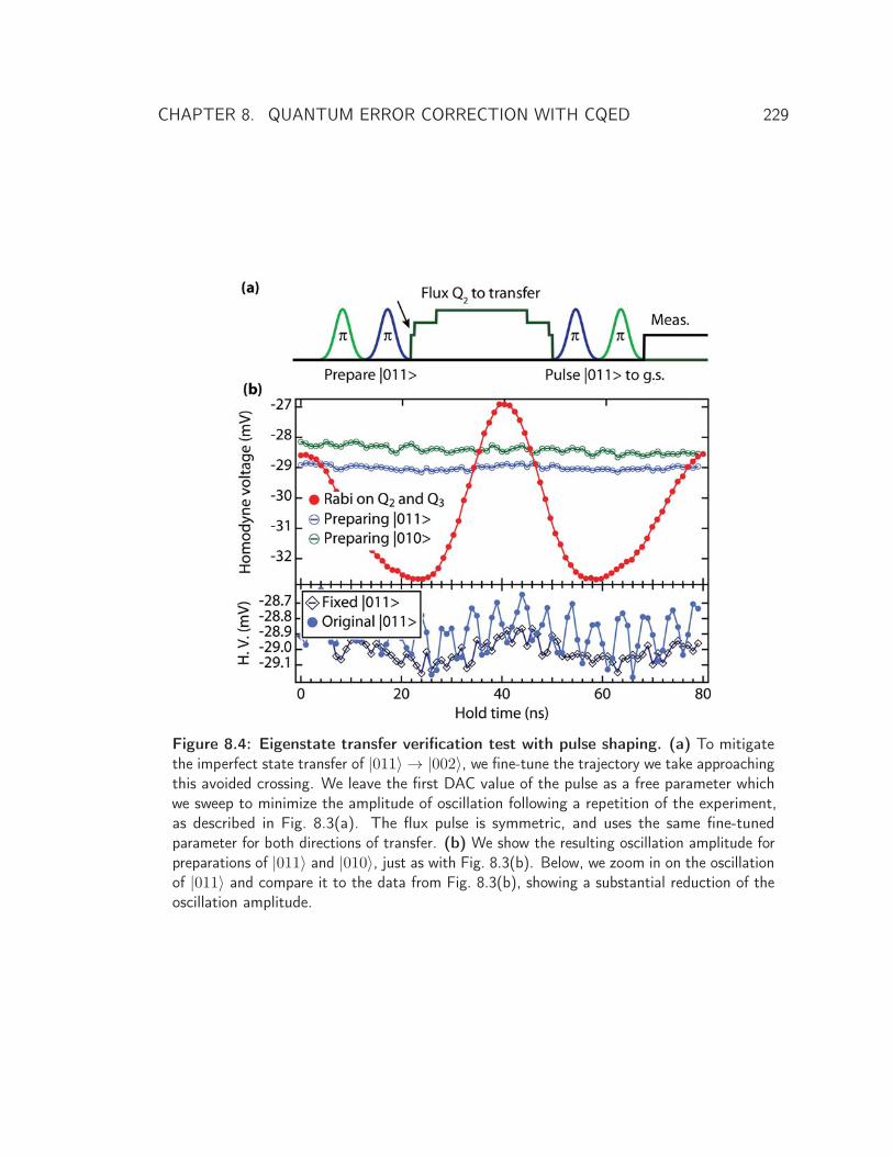
CHAPTER 8. QUANTUM ERROR CORRECTION WITH CQED 229
Figure 8.4: Eigenstate transfer verification test with pulse shaping. (a) To mitigatethe imperfect state transfer of |011〉 → |002〉, we fine-tune the trajectory we take approachingthis avoided crossing. We leave the first DAC value of the pulse as a free parameter whichwe sweep to minimize the amplitude of oscillation following a repetition of the experiment,as described in Fig. 8.3(a). The flux pulse is symmetric, and uses the same fine-tunedparameter for both directions of transfer. (b) We show the resulting oscillation amplitude forpreparations of |011〉 and |010〉, just as with Fig. 8.3(b). Below, we zoom in on the oscillationof |011〉 and compare it to the data from Fig. 8.3(b), showing a substantial reduction of theoscillation amplitude.

CHAPTER 8. QUANTUM ERROR CORRECTION WITH CQED 230
|102〉
|003〉|110〉
⊗ |1〉|200
〉 ⊗|1〉|012〉
|021〉
|030〉 |111〉
|120〉 |201〉
|210〉 |300
〉
Figure 8.5: Calculated spectrum and time-domain measurements of the |102〉 ↔|003〉 avoided crossing. The spectrum of triply-excited states showing the avoided crossingbetween |102〉 and |003〉 as a function of the flux bias on Q1 is characterized in the sameway as in Fig. 8.2. |102〉 is prepared by first making |111〉 and then performing the swapas described in Fig. 8.4. As before, the relevant eigenstates are highlighted in blue. Manyadditional eigenstates (shown in gray) are close in energy but are irrelevant because theydo not interact with the populated states. The large avoided crossing between |102〉 and|003〉 that is used to produce an adiabatic three-qubit interaction happens near 28 mΦ0.Extra lines near 31 mΦ0 and 29 mΦ0 are due to higher-order interactions predicted by theHamiltonian (|102〉 with |030〉 and |003〉 with |111〉), as is the larger first-order interactionat 25 mΦ0 (|102〉 with a hybridization of |021〉 and |111〉), but their impact on the gateprotocol is negligible. (Figure used with permission from [201]. See Copyright Permissions.)
spectroscopy sequence. We show this exact result in Fig. 8.4, thus reducing the amplitudeof spurious oscillation by a factor of three with this simple modification. Additionally, thischange does not worsen the non-adiabaticity of the |010〉 state approaching |001〉.

CHAPTER 8. QUANTUM ERROR CORRECTION WITH CQED 231
8.1.3 |102〉 � |003〉 interaction
Now that we are able to efficiently transfer |111〉 into |102〉, we can turn on the interactionwith |003〉 to acquire three-qubit phase. We show the energy levels in the vicinity of the|102〉 ↔ |003〉 avoided crossing in Fig. 8.5(a), calculated, as before, with a numericaldiagonalization of the system Hamiltonian. We highlight the relevant states, |102〉 and|003〉, in blue. In contrast to the previous plot which showed states with only twoexcitations, there is now a vast proliferation of nearly-degenerate states, shown in gray.We label each state. Note how the slope of each line is approximately proportional to theexcitation of Q1 (the qubit being tuned). Several of these states have finite coupling toour populated states, though the coupling is high-order and therefore very weak.
We can demonstrate the coupling, as before, with swap spectroscopy. We preparethe state |102〉 following the procedure we worked out in the previous section. After wehave moved to the final position F of Q2, we suddenly move Q1 up in frequency, waitsome time, flux back, undo the preparation of |102〉, and measure. If our state leaks intosome other eigenstate during the wait time, our process mapping |102〉 → |000〉 at theend will not address that population and our measurement will indicate that the qubitmanifold is excited. In Fig. 8.5(b) we show the result of performing this measurementover the same range as (a). The primary feature is a large avoided crossing at 27.5 mΦ0,which corresponds precisely with the location of where we expect |102〉 and |003〉 to bein resonance. The splitting is extremely large, at 121 MHz. The size of this crossing isalso reflected in the asymmetry of the coloring: the contrast on the lower-frequency side issmaller than on the larger-frequency side because we are more sudden the further we jump.
We see several other features in the swap spectrogram. At 25 mΦ0 we have anotherfairly large (∼ 35 MHz) crossing, corresponding to an interaction between the state |102〉and a hybridization of |021〉 and |111〉. This region is clearly very complicated, giventhe simultaneous interaction of several states. Moreover, because we are not completelysudden to the crossing of |102〉 and |003〉, |102〉 is likely not fully populated at this point.The contrast of that chevron will be reduced by the fraction of population not in |102〉,though the frequency and location of the oscillation will be unchanged. We also see threemore faint lines, with two near 31 mΦ0 and the third at 29 mΦ0. These correspond tointeractions of |102〉 with |030〉, the residual population of |111〉 with |200〉 ⊗ |1〉 (thesecond excited state of Q1 plus one photon in the cavity), and |003〉 with |111〉.
The fact that these last two interactions are visible is a bit surprising. In the first
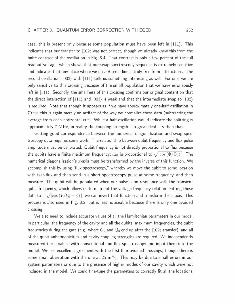
CHAPTER 8. QUANTUM ERROR CORRECTION WITH CQED 232
case, this is present only because some population must have been left in |111〉. Thisindicates that our transfer to |102〉 was not perfect, though we already knew this from thefinite contrast of the oscillation in Fig. 8.4. That contrast is only a few percent of the fullreadout voltage, which shows that our swap spectroscopy sequence is extremely sensitiveand indicates that any place where we do not see a line is truly free from interactions. Thesecond oscillation, |003〉 with |111〉 tells us something interesting as well. For one, we areonly sensitive to this crossing because of the small population that we have erroneouslyleft in |111〉. Secondly, the smallness of this crossing confirms our original contention thatthe direct interaction of |111〉 and |003〉 is weak and that the intermediate swap to |102〉is required. Note that though it appears as if we have approximately one-half oscillation in70 ns, this is again merely an artifact of the way we normalize these data (subtracting theaverage from each horizontal cut). While a half-oscillation would indicate the splitting isapproximately 7 MHz, in reality the coupling strength is a great deal less than that.
Getting good correspondence between the numerical diagonalization and swap spec-troscopy data requires some work. The relationship between qubit frequency and flux pulseamplitude must be calibrated. Qubit frequency is not directly proportional to flux becausethe qubits have a finite maximum frequency; ω01 is proportional to
√|cos (Φ/Φ0) |. Thenumerical diagonalization’s x-axis must be transformed by the inverse of this function. Weaccomplish this by using “flux spectroscopy,” whereby we move the qubit to some locationwith fast-flux and then send in a short spectroscopy pulse at some frequency, and thenmeasure. The qubit will be populated when our pulse is on resonance with the transientqubit frequency, which allows us to map out the voltage-frequency relation. Fitting thosedata to a
√|cos (V/V0 + φ) |, we can invert that function and transform the x-axis. Thisprocess is also used in Fig. 8.2, but is less noticeable because there is only one avoidedcrossing.
We also need to include accurate values of all the Hamiltonian parameters in our model.In particular, the frequency of the cavity and all the qubits’ maximum frequencies, the qubitfrequencies during the gate (e.g. where Q2 and Q3 end up after the |102〉 transfer), and allof the qubit anharmonicities and cavity coupling strengths are required. We independentlymeasured these values with conventional and flux spectroscopy and input them into themodel. We see excellent agreement with the first four avoided crossings, though there issome small aberration with the one at 25 mΦ0. This may be due to small errors in oursystem parameters or due to the presence of higher modes of our cavity which were notincluded in the model. We could fine-tune the parameters to correctly fit all the locations,
CHAPTER 8. QUANTUM ERROR CORRECTION WITH CQED 233
but that process is a bit unscientific. Nevertheless, the quality of correspondence indicatesthat our simple Hamiltonian accurately models the system even for these relatively highlyexcited states.
Now that we have mapped out the flux spectrum of the |102〉 state, it is straightforwardto acquire three-qubit phase. We adiabatically move Q1 up in frequency to move |102〉close to resonance with the |003〉 state. As in the case of the adiabatic two-qubit gate,|102〉 experiences a frequency shift relative to its constituents (|100〉 plus |002〉) due tothe avoided crossing, thus yielding three-qubit phase. In principle this phase could also beacquired suddenly, but the size of the avoided crossing is too large for our room temperatureelectronics to approach. Moreover, the large size makes an adiabatic approach both easyand fast. We can acquire π three-qubit phase in only 20 ns, tuning with the location ofthe closest approach. We might also be concerned that being adiabatic would give usproblems with the three spurious avoided crossings we found along the way. Fortunately,however, these are so small that even while we are adiabatic to |102〉-|003〉, we will besudden to these other interactions, making them wholly irrelevant.
8.1.4 Two-qubit phases
We have now seen how the combination of a sudden transfer to |102〉 and an adiabaticinteraction with |003〉 can give us full control over the three-qubit phase φ111. But, as wediscussed in section 8.1.1, there are three more two-qubit phases that describe a three-qubitphase gate. These phases, φ101, φ011, and φ110, must be dealt with as well. Fortunately,because we reset or measure the ancilla qubits at the end of the QEC code, conditionalphase between those qubits does not matter. Moreover, the code is entirely symmetricwith respect to the qubits until the correction step (and with the exception of the very firstsingle-qubit pulses), so we can use whichever two qubits are most convenient for ancillas.For reasons that will soon become clear, we choose Q1 and Q3. Thus, the value of φ101 isinconsequential and we need only to control φ011 and φ110.
In order to tune-up the remaining two phases, we need to find a location where we willvery rapidly acquire the relevant two-qubit phase so we can control it by changing someparameter by a small amount. It is important that this small adjustment does not changethe other two- or three-qubit phases significantly. Otherwise, it would be difficult to finda location where all of our conditions are simultaneously satisfied. That is, we might beable to get φ110 = 0, but then find that φ111 �= π, so we tune that back up, but then
CHAPTER 8. QUANTUM ERROR CORRECTION WITH CQED 234
φ110 might be wrong again, and so on. While this process may eventually converge withsufficient iterations, it would be time consuming and laborious.
To our great fortune, there is automatically such a point in this gate where the phaseφ011 is acquired rapidly. After we have transferred the population of |011〉 to |002〉 and|111〉 to |102〉, we move to a point positively detuned from that crossing, where thetransition frequency of Q2 is even closer to Q3. At that point, the state |x11〉 is detunedfrom |x02〉 (x = 0, 1) by approximately 100 MHz, and so the phase φ011 is wrappingextremely rapidly. While we do not necessarily have much freedom to control the amountof time we wait at this location (the minimum time is set by making φ111 = π andwe would not want to wait any longer than necessary), we do have a large amount offreedom in choosing the exact frequency to which we tune Q2 (using the language of theprevious subsection on finite bandwidth, we are choosing the location of point F ). Byfinely adjusting this, we change the difference in the energy of |x11〉 and |x02〉 and socontrol the conditional phase. Moreover, since we acquire φ111 adiabatically, this changedoesn’t do much to the other two conditional phases. Therefore, it is fairly insensitive tothe exact location of the |102〉 − |003〉 avoided crossing; Q1 need not get very close toQ2 during the process and so will not interact strongly.
We are not quite as lucky in regard to the remaining phase φ110. The qubits Q1 andQ2 are only close together when we are acquiring three-qubit phase, so we cannot finetune their interaction there independently. Instead, we must append an extra controlledinteraction between these qubits to control their mutual phase. In principle, we could dothis correction suddenly by going on a revolution at the exact detuning from the avoidedcrossing that cancels the spurious phase (as described in section 7.2.2); in practice, however,this is too much trouble since we would need to choose a different pulse detuning andduration every time φ110 changes, which it does frequently during the tune-up process.We instead perform this interaction adiabatically so we can adjust the phase by simplychanging the minimum detuning between Q1 and Q2. Since the uncorrected phase φ110
turns out to be small, we can save time by performing a π pulse on Q2 prior to the adiabaticinteraction, so the phase evolves in the opposite direction and we need not phase-wrap.At this point, it is clear why we chose to ignore the φ101 phase. Those two qubits are notnearest-neighbors so bringing them close to each other to control their conditional phasewould inexorably cause large changes in the other conditional phases.
CHAPTER 8. QUANTUM ERROR CORRECTION WITH CQED 235
8.1.5 Pulse sequence and the cRamsey phase tune-up procedure
We now have all the ingredients of the efficient Toffoli-sign gate. Before we continue,let us briefly recap our decisions thus far. The gate is initiated by suddenly transferring|011〉 to |002〉 and |111〉 to |102〉 with a flux pulse on Q2. The first nanosecond of thetransfer is fine-tuned to compensate for our finite control bandwidth and time resolution.We then wait in the state |102〉, and choose the location of Q2 during this time to set thefirst of our two-qubit phases φ011 = 0. Simultaneously, we move Q1 up in frequency tobring the state |102〉 close to an avoided crossing with |003〉. This causes the energy of|102〉 to diverge from the sum of its components, |100〉 and |002〉, giving us a three-qubitconditional phase. We tune this to equal π by adjusting the time and the detuning ofthis pulse. Moving Q1 back to its home position, we then reverse the swap, dumping theamplitude of |102〉 back into |111〉 (and |002〉 back to |011〉). Finally, we perform a π
pulse on Q2 and adiabatically move Q1 up to bring the states |11x〉 close to resonancewith |02x〉, thus fixing the φ110 conditional phase. A cartoon depicting the resulting pulsesequence is shown in Fig. 8.6.
Looking at the pulse sequence, it is clear that there are quite a few parameters thatwe need to experimentally measure in order to perform this gate. First of all, we needto know precisely what voltage we must apply to our flux line to bring the |111〉 stateinto resonance with |102〉 as well as approximately how long we need to wait to efficientlytransfer our quantum amplitude. Swap spectroscopy is the best way of doing this, as waspreviously shown in Fig. 8.2. We also need to fine-tune the transfer to |102〉, which isdone by repeatedly measuring the oscillation in population while waiting at position F , asshown in Fig. 8.4. We also measure swap spectrograms for all other computational statepreparations as a function of the frequency of Q2 to make sure there aren’t any unknowninteractions that are approaching. We also need to approximate the distance we need tomove Q1 up to acquire three-qubit phase, and verify the absence of any extra crossingsthat affect our other basis states. To do this, we again perform swap spectroscopy for the|111〉 state, as shown in Fig. 8.5. In principle, we have now proven that we can acquirethree-qubit phase, though we still need to work out how to go about measuring it andother conditional phases.
How do we measure these conditional phases? In the previous chapter, we mentionedthat a modified Ramsey oscillation can be used to measure the conditional phase betweentwo qubits. In this sequence, we prepare one of our qubits along the equator of the Bloch
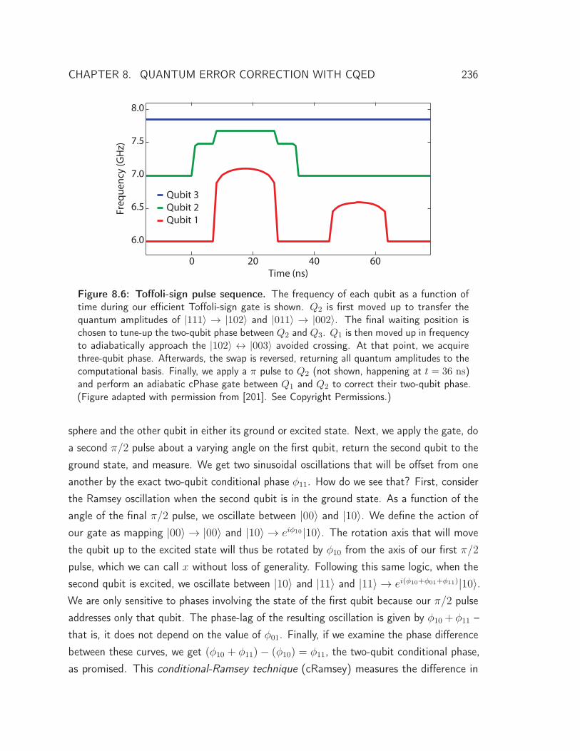
CHAPTER 8. QUANTUM ERROR CORRECTION WITH CQED 236
Figure 8.6: Toffoli-sign pulse sequence. The frequency of each qubit as a function oftime during our efficient Toffoli-sign gate is shown. Q2 is first moved up to transfer thequantum amplitudes of |111〉 → |102〉 and |011〉 → |002〉. The final waiting position ischosen to tune-up the two-qubit phase between Q2 and Q3. Q1 is then moved up in frequencyto adiabatically approach the |102〉 ↔ |003〉 avoided crossing. At that point, we acquirethree-qubit phase. Afterwards, the swap is reversed, returning all quantum amplitudes to thecomputational basis. Finally, we apply a π pulse to Q2 (not shown, happening at t = 36 ns)and perform an adiabatic cPhase gate between Q1 and Q2 to correct their two-qubit phase.(Figure adapted with permission from [201]. See Copyright Permissions.)
sphere and the other qubit in either its ground or excited state. Next, we apply the gate, doa second π/2 pulse about a varying angle on the first qubit, return the second qubit to theground state, and measure. We get two sinusoidal oscillations that will be offset from oneanother by the exact two-qubit conditional phase φ11. How do we see that? First, considerthe Ramsey oscillation when the second qubit is in the ground state. As a function of theangle of the final π/2 pulse, we oscillate between |00〉 and |10〉. We define the action ofour gate as mapping |00〉 → |00〉 and |10〉 → eiφ10 |10〉. The rotation axis that will movethe qubit up to the excited state will thus be rotated by φ10 from the axis of our first π/2pulse, which we can call x without loss of generality. Following this same logic, when thesecond qubit is excited, we oscillate between |10〉 and |11〉 and |11〉 → ei(φ10+φ01+φ11)|10〉.We are only sensitive to phases involving the state of the first qubit because our π/2 pulseaddresses only that qubit. The phase-lag of the resulting oscillation is given by φ10 + φ11 –that is, it does not depend on the value of φ01. Finally, if we examine the phase differencebetween these curves, we get (φ10 + φ11) − (φ10) = φ11, the two-qubit conditional phase,as promised. This conditional-Ramsey technique (cRamsey) measures the difference in
CHAPTER 8. QUANTUM ERROR CORRECTION WITH CQED 237
phase acquired by a single qubit depending on the state of the other qubit during someprocess.
What happens when we apply cRamsey to three qubits? If we only excite two qubits,the above description remains unchanged. We can therefore use this technique withoutmodification to measure and tune-up the two two-qubit phases of the gate. Measuring thethree-qubit phase is more complicated, however. Consider what happens if we perform aRamsey sequence on Q2 with Q1 excited and Q3 excited or not, as described in Fig. 8.7.The first oscillation will be between |100〉 and |110〉, and tells us φ010 + φ110. The secondoscillation is between |101〉 and |111〉, giving us φ010 + φ110 + φ011 + φ111. Subtractingthese two, we see the phase delay is given by φ011 + φ111. This indicates that we cannotonly measure the three-qubit phase in which we are interested. Unfortunately, the onlymeans to circumvent this is to independently measure φ011.
The cRamsey technique provides another important piece of information about yourgate: its approximate fidelity. The contrast of the Ramsey curves after a gate, normalizedto a Ramsey where nothing happens between the two π/2 pulses, is given by the remainingcoherence of the target qubit. Contrast can be reduced if quantum amplitude leaks outof the Hilbert space or for any other reason that the control qubits are not returned totheir ground state. Almost nothing except technical problems with the measurementapparatus will increase contrast. This is a good first test; measuring the ratio of Ramseycontrast is much faster than the more formal methods determining gate fidelity (such asquantum process tomography), so verifying with this method before proceeding with thosetechniques can prevent a lot of wasted effort.
With the two techniques of swap spectroscopy and cRamsey, we can fully tune-up theToffoli-sign gate. After extracting the parameters from swap spectroscopy as describedabove, we tune-up the phases φ011 by adjusting the waiting position of Q2, represented bythe flat portion of the green curve in Fig. 8.6. Since we acquire phase so rapidly at thatposition, there are usually several waiting locations that will satisfy φ011 = 0, which wechoose between experimentally to maximize the Ramsey contrast of the other basis states.We set φ111 with the height of the first pulse on Q1 (the red curve). Finally, we adjustφ110 with the height of the second pulse on Q1. This tune-up is iterated several times untilall the phase values are stable. Given that, we can also measure the single-qubit phasesfor unwrapping in software.

CHAPTER 8. QUANTUM ERROR CORRECTION WITH CQED 238
Red:
Blue:
Green:
Aga
te
Aco
ntro
l
010 + 110+ 011+ 111 010 + 110
(a)
(b)
Q1 Q3 Q2 Q2 Q3 Q1Gate / no gate
X X
X
X X
X
X
X X X
X
X X
X
X
X
Figure 8.7: Conditional-Ramsey phase tune-up sequence for measuring φ111+φ011.(a) The pulse sequence for three Ramsey experiments is shown. For red and green, asuperposition of the states |101〉 and |111〉 is prepared; a superposition of |100〉 and |110〉 ismade for blue. The Toffoli gate we are testing is applied to the red and blue cases. After each,a π/2 pulse around the φ-axis is applied to Q2, and, before being measured, the remainingqubits are pulsed back to their ground states. This procedure tells us the phase differencebetween the two prepared states. In red, we measure the phase φ010 + φ110 + φ011 + φ111;in blue, we measure φ010 + φ110. Subtracting the two will give us the value of φ111 + φ011,which, combined with similar experiments with different qubit preparations, fully specifies theccPhase gate. We are not interested in the phase of the green experiment in this case, butthe amplitude of oscillation indicates any loss in fidelity. (b) The result of performing theexperiment described in (a). We indicate the phase delays of the red and blue experimentswhich we fit and subtract from one another to extract φ111 + φ011. We also highlight theamplitudes of the red and green experiments. Ideally, these amplitudes should be identical,which would indicate that the gate is working properly. Additional decoherence because ofbeing highly excited and imperfect state transfer slightly reduces the amplitude of red byabout 4%.

CHAPTER 8. QUANTUM ERROR CORRECTION WITH CQED 239
π-ccPhase
Rπ/2xRπ/2
x Rπx
ccNOT
Figure 8.8: ccNOT implemented with Toffoli-sign gate. The full pulse sequence forgenerating a controlled-controlled-NOT gate with our efficient Toffoli-sign gate is shown. Q2
is pulsed by π/2 around the x-axis before the Toffoli-sign gate is applied. Because of our πpulse on Q2 to save time on the unwrapping of the φ011 phase, we refer to this operation asa π-ccPhase. Afterwards, another π/2 gate is applied to Q2. If the ccPhase flipped the signof the manifold, this gate will combine with the other rotations on Q2 to flip its state. If not,it will rotate Q2 back to its original value. (Figure used with permission from [201]. SeeCopyright Permissions.)
8.1.6 Toffoli-sign gate tomography
We first demonstrate our tuned-up gate by measuring its classical action. The ccPhasegate, which maps |111〉 to −|111〉, has no effect on pure computational states becausethe extra phase acts globally. Instead, we can implement a ccNOT gate by appending±π/2 pulses on Q2 both before and after a ccPhase gate, in the same way that we havepreviously mapped a cPhase to a cNOT. For the two input states where both ancillas areexcited (|101〉, |111〉, becoming |101〉 ± |111〉 after the pulse), Q2 acquires a π phaseshift which flips the phase of the second pulse, and so the two pulses combine for a fullrotation. (The uncorrected φ101 phase is irrelevant because it does not affect Q2.) Othercomputational states do not see the phase of Q2 shifted, so the pulses cancel. We showthe actual phase in the shaded region of Fig. 8.8, which differs slightly from a pure ccPhasebecause of the π pulse used to speed the unwrapping of φ110. A ccNOT is thus constructedby making both the pre- and post-rotations a positive π/2 rotation.
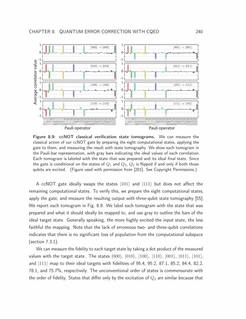
CHAPTER 8. QUANTUM ERROR CORRECTION WITH CQED 240
|000〉 → |000〉
|010〉 → |010〉
|100〉 → |100〉
|110〉 → |110〉
|001〉 → |001〉
|011〉 → |011〉
|101〉 → |111〉
|111〉 → |101〉Aver
age
corr
elat
or v
alue
IIX
IIY
YZZ
XZZ
ZYZ
YYZ
XYZ
ZXZ
YXZ
XXZ
ZZY
YZY
XZY
ZYY
YYY
XYY
ZXY
YXY
XXY
ZZX
YZX
XZX
ZYX
YYX
XYX
ZXX
YXX
XXX
ZZI
YZI
XZI
ZYI
YYI
ZXI
YXI
XXI
ZIZ
YIZ
XIZ
ZIY
YIY
XIY
ZIX
YIX
XIX
IZZ
IYZ
IXZ
IZY
IYY
IXY
IZX
IYX
IXX
ZII
YII
XII
IZI
IYI
IXI
IIZ
ZZZ
XYI
Pauli operator
IIX
IIY
YZZ
XZZ
ZYZ
YYZ
XYZ
ZXZ
YXZ
XXZ
ZZY
YZY
XZY
ZYY
YYY
XYY
ZXY
YXY
XXY
ZZX
YZX
XZX
ZYX
YYX
XYX
ZXX
YXX
XXX
ZZI
YZI
XZI
ZYI
YYI
ZXI
YXI
XXI
ZIZ
YIZ
XIZ
ZIY
YIY
XIY
ZIX
YIX
XIX
IZZ
IYZ
IXZ
IZY
IYY
IXY
IZX
IYX
IXX
ZII
YII
XII
IZI
IYI
IXI
IIZ
ZZZ
XYI
Pauli operator
Figure 8.9: ccNOT classical verification state tomograms. We can measure theclassical action of our ccNOT gate by preparing the eight computational states, applying thegate to them, and measuring the result with state tomography. We show each tomogram inthe Pauli-bar representation, with gray bars indicating the ideal values of each correlation.Each tomogram is labeled with the state that was prepared and its ideal final state. Sincethe gate is conditional on the states of Q1 and Q3, Q2 is flipped if and only if both thosequbits are excited. (Figure used with permission from [201]. See Copyright Permissions.)
A ccNOT gate ideally swaps the states |101〉 and |111〉 but does not affect theremaining computational states. To verify this, we prepare the eight computational states,apply the gate, and measure the resulting output with three-qubit state tomography [55].We report each tomogram in Fig. 8.9. We label each tomogram with the state that wasprepared and what it should ideally be mapped to, and use gray to outline the bars of theideal target state. Generally speaking, the more highly excited the input state, the lessfaithful the mapping. Note that the lack of erroneous two- and three-qubit correlationsindicates that there is no significant loss of population from the computational subspace(section 7.3.1).
We can measure the fidelity to each target state by taking a dot product of the measuredvalues with the target state. The states |000〉, |010〉, |100〉, |110〉, |001〉, |011〉, |101〉,and |111〉 map to their ideal targets with fidelities of 95.4, 95.2, 87.1, 85.2, 84.4, 82.2,78.1, and 75.7%, respectively. The unconventional order of states is commensurate withthe order of fidelity. States that differ only by the excitation of Q2 are similar because that
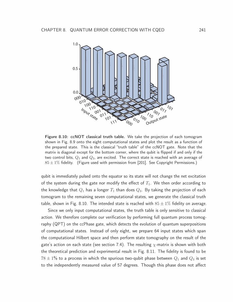
CHAPTER 8. QUANTUM ERROR CORRECTION WITH CQED 241
011Input state
Output state
101011001110100010000
010100
110001
101111
0000.0
1.0
0.5
Figure 8.10: ccNOT classical truth table. We take the projection of each tomogramshown in Fig. 8.9 onto the eight computational states and plot the result as a function ofthe prepared state. This is the classical “truth table” of the ccNOT gate. Note that thematrix is diagonal except for the bottom corner, where the qubit is flipped if and only if thetwo control bits, Q1 and Q3, are excited. The correct state is reached with an average of85 ± 1% fidelity. (Figure used with permission from [201]. See Copyright Permissions.)
qubit is immediately pulsed onto the equator so its state will not change the net excitationof the system during the gate nor modify the effect of T1. We then order according tothe knowledge that Q1 has a longer T1 than does Q3. By taking the projection of eachtomogram to the remaining seven computational states, we generate the classical truthtable, shown in Fig. 8.10. The intended state is reached with 85 ± 1% fidelity on average.
Since we only input computational states, the truth table is only sensitive to classicalaction. We therefore complete our verification by performing full quantum process tomog-raphy (QPT) on the ccPhase gate, which detects the evolution of quantum superpositionsof computational states. Instead of only eight, we prepare 64 input states which spanthe computational Hilbert space and then perform state tomography on the result of thegate’s action on each state (see section 7.4). The resulting χ-matrix is shown with boththe theoretical prediction and experimental result in Fig. 8.11. The fidelity is found to be78 ± 1% to a process in which the spurious two-qubit phase between Q1 and Q3 is setto the independently measured value of 57 degrees. Though this phase does not affect
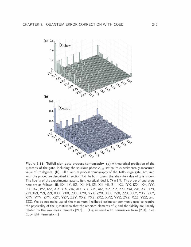
CHAPTER 8. QUANTUM ERROR CORRECTION WITH CQED 242
Figure 8.11: Toffoli-sign gate process tomography. (a) A theoretical prediction of theχ-matrix of the gate, including the spurious phase φ101 set to its experimentally-measuredvalue of 57 degrees. (b) Full quantum process tomography of the Toffoli-sign gate, acquiredwith the procedure described in section 7.4. In both cases, the absolute value of χ is shown.The fidelity of the experimental gate to its theoretical ideal is 78±1%. The order of operatorshere are as follows: III, IIX, IIY, IIZ, IXI, IYI, IZI, XII, YII, ZII, IXX, IYX, IZX, IXY, IYY,IZY, IXZ, IYZ, IZZ, XIX, YIX, ZIX, XIY, YIY, ZIY, XIZ, YIZ, ZIZ, XXI, YXI, ZXI, XYI, YYI,ZYI, XZI, YZI, ZZI, XXX, YXX, ZXX, XYX, YYX, ZYX, XZX, YZX, ZZX, XXY, YXY, ZXY,XYY, YYY, ZYY, XZY, YZY, ZZY, XXZ, YXZ, ZXZ, XYZ, YYZ, ZYZ, XZZ, YZZ, andZZZ. We do not make use of the maximum-likelihood estimator commonly used to requirethe physicality of the χ-matrix so that the reported elements of χ and the fidelity are linearlyrelated to the raw measurements [216]. (Figure used with permission from [201]. SeeCopyright Permissions.)
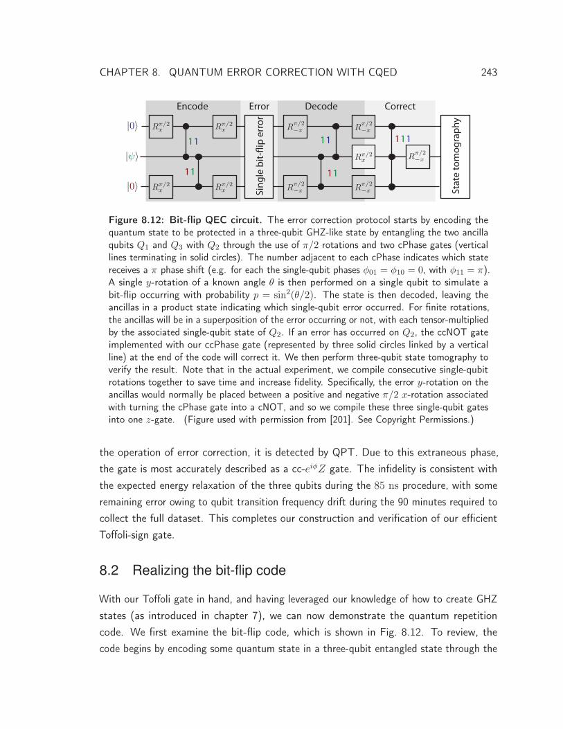
CHAPTER 8. QUANTUM ERROR CORRECTION WITH CQED 243
Sing
le b
it-fli
p er
ror
Stat
e to
mog
raph
y
111
Encode Error Decode Correct
11
11
11
11
Rπ/2x Rπ/2
x
Rπ/2xRπ/2
x Rπ/2−x R
π/2−x
Rπ/2−x R
π/2−x
Rπ/2−xRπ/2
x|ψ〉
|0〉
|0〉
Figure 8.12: Bit-flip QEC circuit. The error correction protocol starts by encoding thequantum state to be protected in a three-qubit GHZ-like state by entangling the two ancillaqubits Q1 and Q3 with Q2 through the use of π/2 rotations and two cPhase gates (verticallines terminating in solid circles). The number adjacent to each cPhase indicates which statereceives a π phase shift (e.g. for each the single-qubit phases φ01 = φ10 = 0, with φ11 = π).A single y-rotation of a known angle θ is then performed on a single qubit to simulate abit-flip occurring with probability p = sin2(θ/2). The state is then decoded, leaving theancillas in a product state indicating which single-qubit error occurred. For finite rotations,the ancillas will be in a superposition of the error occurring or not, with each tensor-multipliedby the associated single-qubit state of Q2. If an error has occurred on Q2, the ccNOT gateimplemented with our ccPhase gate (represented by three solid circles linked by a verticalline) at the end of the code will correct it. We then perform three-qubit state tomography toverify the result. Note that in the actual experiment, we compile consecutive single-qubitrotations together to save time and increase fidelity. Specifically, the error y-rotation on theancillas would normally be placed between a positive and negative π/2 x-rotation associatedwith turning the cPhase gate into a cNOT, and so we compile these three single-qubit gatesinto one z-gate. (Figure used with permission from [201]. See Copyright Permissions.)
the operation of error correction, it is detected by QPT. Due to this extraneous phase,the gate is most accurately described as a cc-eiφZ gate. The infidelity is consistent withthe expected energy relaxation of the three qubits during the 85 ns procedure, with someremaining error owing to qubit transition frequency drift during the 90 minutes required tocollect the full dataset. This completes our construction and verification of our efficientToffoli-sign gate.
8.2 Realizing the bit-flip code
With our Toffoli gate in hand, and having leveraged our knowledge of how to create GHZstates (as introduced in chapter 7), we can now demonstrate the quantum repetitioncode. We first examine the bit-flip code, which is shown in Fig. 8.12. To review, thecode begins by encoding some quantum state in a three-qubit entangled state through the
CHAPTER 8. QUANTUM ERROR CORRECTION WITH CQED 244
use of cPhase gates. This is an exact replica of the code we used to create GHZ statesin chapter 7, but now modified so the state of Q2 is arbitrary. (When Q2 is located onthe equator, the resulting state is a maximally-entangled GHZ state [55, 70, 252]; for anyother state, the resulting state may or may not exhibit some level of entanglement.) Asbefore, we use the sudden cPhase gates that employ the |11〉 ↔ |02〉 avoided crossingbetween the involved qubits. The state α|0〉 + β|1〉 is thus encoded as α|000〉 + β|111〉.
Recall that this state has the property that any two-qubit ZZ product is +1 regardlessof the values of α and β. Moreover, if any single qubit is flipped, one or both of theseZZ products will flip this sign as well. For example, if Q3 were flipped, we will have thestate α|001〉 + β|110〉, whose Z1Z2 expectation value is +1 but whose Z2Z3 productis −1. As seen in table 2.1, if no more than one qubit flips, knowledge of the two ZZ
products uniquely specifies which error occurred. Since we do not have extra ancilla qubitsto extract these error syndromes in a fault-tolerant way, we instead reverse the encoding,leaving Q2 in a state that may or may not have been flipped and Q1 and Q3 containingthe values of the Z1Z2 and Z2Z3 products (as explained in section 2.3.4). Specifically, ifQ2 were flipped, both of the ancillas will be left in their excited state. As discussed insection 2.3.4, we can then use these qubits as the control bits of our three-qubit Toffoligate to rotate Q2 back to its original state conditional on the error. At this point, theancillas store the entropy associated with the error. If we wished to apply another roundof QEC, we would need to reset them to return the qubit register to its original state,perhaps by using the method described in section 6.2.4. Thus, we see that this code cancorrect for full bit-flips.
8.2.1 Finite rotation errors
With classical bits, the only errors that may occur are full bit-flips, mapping 0 ↔ 1. Withquantum bits, however, finite rotations may occur because superpositions of 0 and 1 areallowed. Luckily, the code we just introduced works for finite errors as well. To show this,we will step through the evolution of the quantum register at each point in the code. Priorto encoding, Q2 is in an unknown state α|0〉 + β|1〉 and the ancilla are in their groundstate, so the system state is |ψ〉 = (α|0〉+ β|1〉)⊗ |00〉, where we list Q2 followed by thetwo-qubit ancilla state of Q1 and Q3. After the encoding step, we are in the canonical state|ψ〉 = α|000〉+β|111〉, which is sensitive to errors. Suppose we now perform a rotation onQ2, not of π, but some finite angle θ. Though we implement this as a coherent rotation,
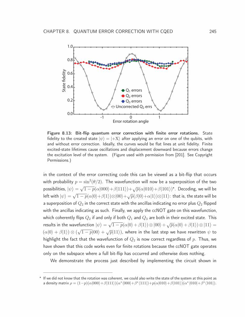
CHAPTER 8. QUANTUM ERROR CORRECTION WITH CQED 245
1.0
0.8
0.6
0.4
0.2
0.0
Stat
e fid
elity
-1 0 1Error rotation angle
Q1 errorsQ2 errorsQ3 errors
Uncorrected Q2 errs
Figure 8.13: Bit-flip quantum error correction with finite error rotations. Statefidelity to the created state |ψ〉 = |+X〉 after applying an error on one of the qubits, withand without error correction. Ideally, the curves would be flat lines at unit fidelity. Finiteexcited-state lifetimes cause oscillations and displacement downward because errors changethe excitation level of the system. (Figure used with permission from [201]. See CopyrightPermissions.)
in the context of the error correcting code this can be viewed as a bit-flip that occurswith probability p = sin2(θ/2). The wavefunction will now be a superposition of the twopossibilities, |ψ〉 = √
1 − p(α|000〉+β|111〉)+√p(α|010〉+β|101〉)∗. Decoding, we will be
left with |ψ〉 = √1 − p(α|0〉+β|1〉)⊗|00〉+√
p(β|0〉+α|1〉)⊗|11〉: that is, the state will bea superposition of Q2 in the correct state with the ancillas indicating no error plus Q2 flippedwith the ancillas indicating as such. Finally, we apply the ccNOT gate on this wavefunction,which coherently flips Q2 if and only if both Q1 and Q3 are both in their excited state. Thisresults in the wavefunction |ψ〉 = √
1 − p(α|0〉+β|1〉)⊗|00〉+√p(α|0〉+β|1〉)⊗|11〉 =
(α|0〉 + β|1〉) ⊗ (√1 − p|00〉 + √
p|11〉), where in the last step we have rewritten ψ tohighlight the fact that the wavefunction of Q2 is now correct regardless of p. Thus, wehave shown that this code works even for finite rotations because the ccNOT gate operatesonly on the subspace where a full bit-flip has occurred and otherwise does nothing.
We demonstrate the process just described by implementing the circuit shown in
∗ If we did not know that the rotation was coherent, we could also write the state of the system at this point asa density matrix ρ = (1−p)(α|000〉+β|111〉)(α∗〈000|+β∗〈111|)+p(α|010〉+β|101〉)(α∗〈010|+β∗〈101|).
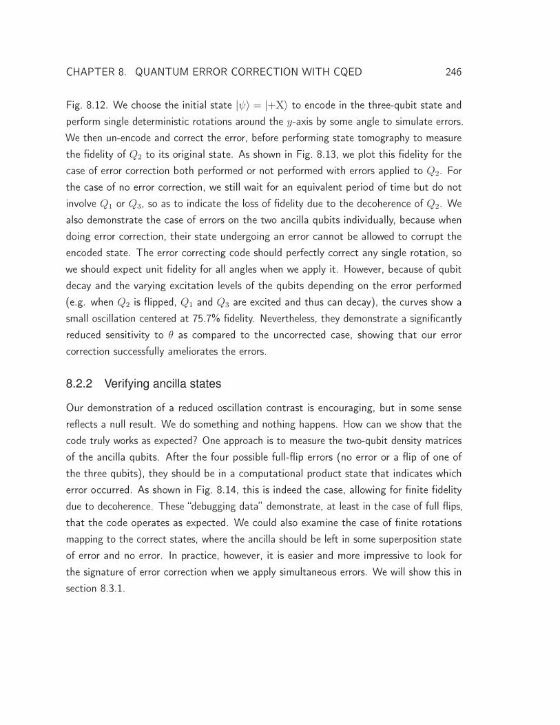
CHAPTER 8. QUANTUM ERROR CORRECTION WITH CQED 246
Fig. 8.12. We choose the initial state |ψ〉 = |+X〉 to encode in the three-qubit state andperform single deterministic rotations around the y-axis by some angle to simulate errors.We then un-encode and correct the error, before performing state tomography to measurethe fidelity of Q2 to its original state. As shown in Fig. 8.13, we plot this fidelity for thecase of error correction both performed or not performed with errors applied to Q2. Forthe case of no error correction, we still wait for an equivalent period of time but do notinvolve Q1 or Q3, so as to indicate the loss of fidelity due to the decoherence of Q2. Wealso demonstrate the case of errors on the two ancilla qubits individually, because whendoing error correction, their state undergoing an error cannot be allowed to corrupt theencoded state. The error correcting code should perfectly correct any single rotation, sowe should expect unit fidelity for all angles when we apply it. However, because of qubitdecay and the varying excitation levels of the qubits depending on the error performed(e.g. when Q2 is flipped, Q1 and Q3 are excited and thus can decay), the curves show asmall oscillation centered at 75.7% fidelity. Nevertheless, they demonstrate a significantlyreduced sensitivity to θ as compared to the uncorrected case, showing that our errorcorrection successfully ameliorates the errors.
8.2.2 Verifying ancilla states
Our demonstration of a reduced oscillation contrast is encouraging, but in some sensereflects a null result. We do something and nothing happens. How can we show that thecode truly works as expected? One approach is to measure the two-qubit density matricesof the ancilla qubits. After the four possible full-flip errors (no error or a flip of one ofthe three qubits), they should be in a computational product state that indicates whicherror occurred. As shown in Fig. 8.14, this is indeed the case, allowing for finite fidelitydue to decoherence. These “debugging data” demonstrate, at least in the case of full flips,that the code operates as expected. We could also examine the case of finite rotationsmapping to the correct states, where the ancilla should be left in some superposition stateof error and no error. In practice, however, it is easier and more impressive to look forthe signature of error correction when we apply simultaneous errors. We will show this insection 8.3.1.
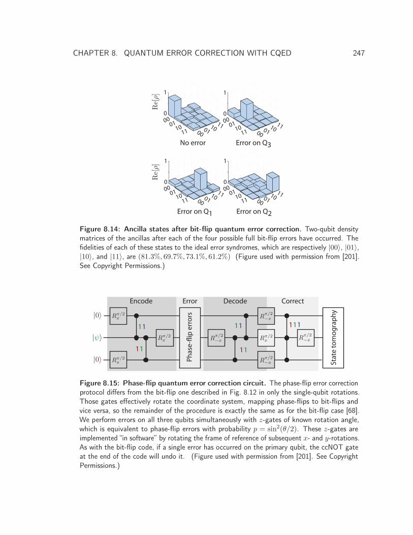
CHAPTER 8. QUANTUM ERROR CORRECTION WITH CQED 247
IIIZ
ZIZZ
IIIZ
ZIZZ
0
1
IIIZ
ZIZZ
IIIZ
ZIZZ
0
1
Error on Q3
Error on Q2Error on Q1
No error
0001
1011 00
0110
11
0
1
IIIZ
ZIZZ
IIIZ
ZIZZ
0
1
IIIZ
ZIZZ
IIIZ
ZIZZ
0
1
0001
1011 00
0110
11
0
1
0001
1011 00
0110
11
0
1
0001
1011 00
0110
11
0
1Re[ρ]
Re[ρ]
Figure 8.14: Ancilla states after bit-flip quantum error correction. Two-qubit densitymatrices of the ancillas after each of the four possible full bit-flip errors have occurred. Thefidelities of each of these states to the ideal error syndromes, which are respectively |00〉, |01〉,|10〉, and |11〉, are (81.3%, 69.7%, 73.1%, 61.2%) (Figure used with permission from [201].See Copyright Permissions.)
Phas
e-fli
p er
rors
Stat
e to
mog
raph
y111
Encode Error Decode Correct
11
11
11
11
Rπ/2x
Rπ/2x
Rπ/2x R
π/2−x
Rπ/2−x
Rπ/2−x
Rπ/2−xRπ/2
x|ψ〉
|0〉
|0〉
Figure 8.15: Phase-flip quantum error correction circuit. The phase-flip error correctionprotocol differs from the bit-flip one described in Fig. 8.12 in only the single-qubit rotations.Those gates effectively rotate the coordinate system, mapping phase-flips to bit-flips andvice versa, so the remainder of the procedure is exactly the same as for the bit-flip case [68].We perform errors on all three qubits simultaneously with z-gates of known rotation angle,which is equivalent to phase-flip errors with probability p = sin2(θ/2). These z-gates areimplemented “in software” by rotating the frame of reference of subsequent x- and y-rotations.As with the bit-flip code, if a single error has occurred on the primary qubit, the ccNOT gateat the end of the code will undo it. (Figure used with permission from [201]. See CopyrightPermissions.)
CHAPTER 8. QUANTUM ERROR CORRECTION WITH CQED 248
8.3 Realizing the phase-flip code
The quantum repetition code can correct for one type of error: bit-flips or phase-flips.Thus far, we have discussed the case of bit-flip errors. These have the advantage of beingintuitive because of their direct classical analog. However, they are in some sense a lessimportant error in our system. Bit errors only occur on their own if we have incorrectlytuned-up pulses (or, perhaps, some spurious mixer leakage, etc). They also happen duringspontaneous emission, but only in combination with phase-flip errors. (That is, the T1
process is not a bit-flip and it can only be described as a combination of bit- and phase-errors; see section 2.1.5.) Phase-flips, on the other hand, are a much more common kind oferror associated with inhomogeneous dephasing (Tφ dephasing not due to T1). Therefore,we are interested in implementing the phase-flip error correcting code. Fortunately, asshown in Fig. 8.15, the phase-flip code is a very straightforward modification of the bit-flipcode. The only difference is in the rotations performed after the entanglement. Ratherthan rotating the primary qubit as in phase-flip correction, the ancillas are π/2 pulsed.This can be understood as a change in coordinate system, converting phase-flips to bit-flipsand vice versa; the remainder of the code is exactly the same as in the previous case[30, 68, 253].
8.3.1 Simultaneous errors
We originally introduced the quantum repetition code in the context of a classical binarysymmetric channel (section 2.3.2). We wished to transmit a bit through a noisy communi-cation channel that had a probability p of flipping it. We found that we could reduce oursensitivity to this error if we communicated each bit three times. The resulting error ratewas a quadratic function of p, given by 3p2 − 2p3. Critically, as long as p was small – lessthan 1/2, which is not a very strict requirement, since a channel with error probability 1/2has zero information carrying capacity – then the overall error rate of this approach wassmaller than sending only one bit. The reason p must be small is that by transmittingmore bits of information, we are also adding ways for the information to be corrupted.
This is also true for quantum error correction. When we add extra qubits to encodeour quantum state, we also add extra ways by which the system could be corrupted. Thequbits we use to encode are no less likely to experience an error than the qubit we are tryingto protect. This idea shows that our demonstration of error correction is quite artificial
CHAPTER 8. QUANTUM ERROR CORRECTION WITH CQED 249
because we intentionally apply exactly one error at a time. A more realistic error modelwould account for the fact that in real physical systems, errors occur at approximately thesame rate on all qubits rather than on one at a time. Our error correction scheme can onlysucceed if no more than error happens, and will fail if there are two or three coincidenterrors. As in the classical case, if we have a single-qubit error rate p, the probability oftwo or more errors is given by 3p2 − 2p3 and so the fidelity of the error correction processshould be given by 1 − 3p2 + 2p3. For a scheme with gate fidelity limited by decoherence,these coefficients will be smaller, but crucially, any linear dependence on p will be stronglysuppressed. If the qubits experience errors at different rates, these coefficients would againbe modified, but the linear dependence would remain abated. This suppression of lineardependence on p is the unambiguous signature of quantum error correction.
8.3.2 Process tomography
We demonstrate the procedure shown in Fig. 8.15 by creating some state |ψ〉 of Q2,applying the protocol, and then measuring the state of Q2 using state tomography. Incontrast to the bit-flip case, we are now going to do something slightly more sophisticated.Instead of testing some specific chosen state |ψ〉 that could be more or less susceptible tothe errors that are being applied, we instead perform full quantum process tomographyon the protocol (section 7.4). To do so, we create four states (|0〉, |1〉, |+X〉 and |+Y 〉)that span the single-qubit Hilbert space of Q2. We apply the QEC circuit to each ofthese states and measure the result with state tomography. The resulting state fidelitiesfor the case of performing or not performing error correction are plotted in the insets ofFig. 8.16. For the case of no error correction, we apply identical single-qubit rotations toQ2 without involving the ancillas. We insert appropriate delays to have the same totalprocedure duration to indicate the infidelity due to the decoherence of Q2, then combineeach of these state tomograms into a single process matrix and calculate the fidelity ofthat process matrix to the identity. The two process fidelities are plotted and fit to apolynomial in Fig. 8.16.
For no error correction, we find a purely linear dependence on error probability givenby f = 0.81 − 0.79p. However, when we apply the correction, we suppress all lineardependence, finding that the data are well-fit by f = 0.76− 1.46p2 +0.72p3. If we includea linear term in this function, its best-fit value is found to be consistent with zero. Thesuppression of linear dependence on p when performing error correction was precisely the
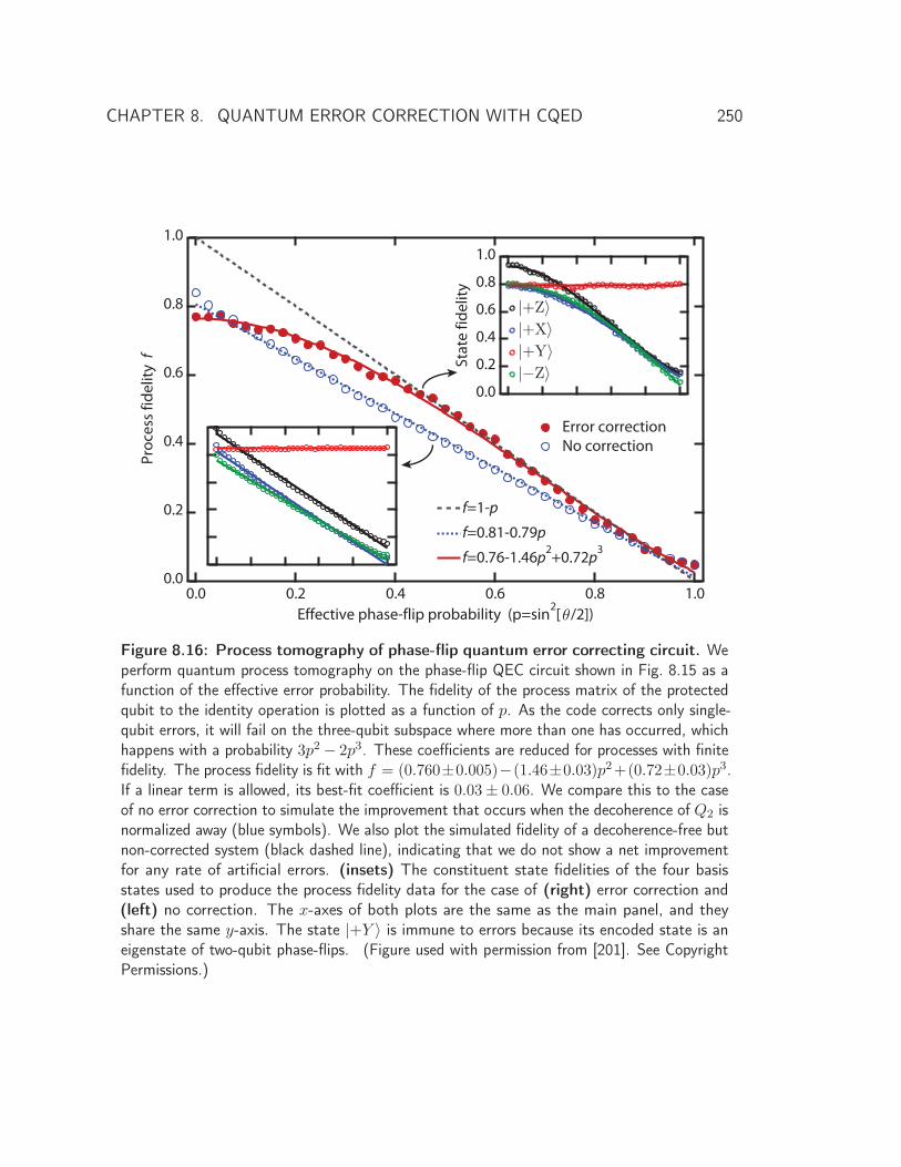
CHAPTER 8. QUANTUM ERROR CORRECTION WITH CQED 250
θ
|+Z〉|+X〉|+Y〉|−Z〉
Figure 8.16: Process tomography of phase-flip quantum error correcting circuit. Weperform quantum process tomography on the phase-flip QEC circuit shown in Fig. 8.15 as afunction of the effective error probability. The fidelity of the process matrix of the protectedqubit to the identity operation is plotted as a function of p. As the code corrects only single-qubit errors, it will fail on the three-qubit subspace where more than one has occurred, whichhappens with a probability 3p2 − 2p3. These coefficients are reduced for processes with finitefidelity. The process fidelity is fit with f = (0.760±0.005)−(1.46±0.03)p2+(0.72±0.03)p3.If a linear term is allowed, its best-fit coefficient is 0.03± 0.06. We compare this to the caseof no error correction to simulate the improvement that occurs when the decoherence of Q2 isnormalized away (blue symbols). We also plot the simulated fidelity of a decoherence-free butnon-corrected system (black dashed line), indicating that we do not show a net improvementfor any rate of artificial errors. (insets) The constituent state fidelities of the four basisstates used to produce the process fidelity data for the case of (right) error correction and(left) no correction. The x-axes of both plots are the same as the main panel, and theyshare the same y-axis. The state |+Y 〉 is immune to errors because its encoded state is aneigenstate of two-qubit phase-flips. (Figure used with permission from [201]. See CopyrightPermissions.)

CHAPTER 8. QUANTUM ERROR CORRECTION WITH CQED 251
signature that we had hoped to find, and proves that the circuit works as expected. Weanticipated that the fidelity of the process would only be improved by error correctionif the error probability was less than 1/2, below which it should be reduced. However,in Fig. 8.16, we see that the error corrected case is always better than the non-errorcorrected case. This is the result of an accident: below 50% fidelity, decoherence of ourstate actually improves our state fidelity since a fully-mixed state has 50% fidelity to anystate. (Its II Pauli correlation is always defined to be +1, and is included in the fidelity.)Moreover, when we are performing quantum error correction, we are much more susceptibleto decoherence since three qubits are involved rather than one. Thus, we get a boost infidelity that pushes us above the uncorrected case. Nevertheless, if the code was perfectand decoherence was nonexistent, when p > 1/2, the protocol should indeed reduce ournet fidelity.
In Fig. 8.16, we also plot the fidelity of a process without error correction in the absenceof any overhead. This simulates a process in which we perfectly prepare some state andimmediately apply an error before measuring the resulting fidelity. As you can see, this lineis always above the experimental lines, which indicates that our error correction protocolnever actually improves effective error rates. Put another way: while the protocol correctserrors, the associated overhead is so large that the net fidelity of some process will neverbe improved. This is not the fault of the code, but rather of the system itself. The qubitswe used in this planar structure are simply too error-prone. Their coherence times were onthe order of 1 μs, which is on the order of the time it takes to run the correction protocol.In order for error correction to make sense, the overhead needs to be small compared tothe improvement associated with going from a linear dependence on p to a quadratic one.Thus, in order to show an actual improvement (and perform error correction for a reasonother than its own sake), we need substantially better qubits.
8.4 Conclusion
In this chapter, we have demonstrated the first realization of the most basic form ofquantum error correction – the quantum repetition code – in a superconducting circuit. Werealized both bit- and phase-flip error correction, testing both major conceptual componentsof the nine-qubit Shor code [17] which can protect from arbitrary single-qubit errors byconcatenating the two codes. The key to our implementation was an efficient three-qubitToffoli-sign gate, which is required for the autonomous repetition code. Our gate made use
CHAPTER 8. QUANTUM ERROR CORRECTION WITH CQED 252
of an avoided crossing between the |102〉 and |003〉 non-computational states to acquirethree-qubit conditional phase. Accessing this avoided crossing required intentionally leavingthe computational space with a sudden swap operation. We characterized our gate withboth quantum state and quantum process tomography, and found fidelities approaching80%. The gate requires approximately half the time of an equivalent construction withone- and two-qubit gates.
Combining this gate with a sudden cPhase gate, we implemented the bit-flip QECcode. We began by encoding the qubit state that we wished to protect in a three-qubitGHZ-like state and then applied a deterministic rotation on one of the qubits to simulate abit-flip error. We showed how the code works with finite error rotations and that the errorsyndromes are being correctly encoded in the ancilla qubits. We also implemented thephase-flip code, but used a more sophisticated error model that simulated simultaneouserrors on all three qubits. We performed process tomography on this circuit, and found theexpected suppression of linear dependence of process fidelity on error probability. Thoughthis proved that the code was working as expected, the fidelity never exceeded the case ofno error correction without overhead, which indicates that the improvement of the fidelityof a real physical process will require significant advances in both gate fidelity and devicecomplexity.
CHAPTER 9
The Tunable 3D cQED Architecture
In the previous chapter, we showed that we have built up the sophistication to performbasic quantum error correction with superconducting qubits. We concluded by noting
that although the circuit worked as anticipated, it did not improve error rates because ourqubits were too short-lived. We need much more coherent qubits that are as controllableas those we have already used. Our answer to this requirement is the tunable 3D cQEDarchitecture, first introduced in section 4.2. That architecture combines the extremelyhigh coherence times of 3D cQED with the ability to tune the system in-situ with fast fluxbias lines. In this chapter, we will summarize the experimental results attained thus farwith tunable 3D cQED. Though the results are unpublished, we aim to give a flavor of thepossibilities enabled by this architecture.
We begin by showing that our flux bias lines constitute a significant relaxation channel.We measure qubit T1 as a function of frequency. Both the magnitude and structure ofthese data provide strong support for our hypothesis that the qubit relaxes through theFBL because of capacitive coupling. We confirm this by adding a low-pass filter to theFBL, and demonstrate that the qubit’s relaxation is significantly ameliorated when wefabricate a big enough filter capacitor. We also use flux spectroscopy to confirm that thislow-pass filter does not adversely affect the response time of our fast flux bias lines.
In the second part of this chapter, we introduce several experiments to measure the
253
CHAPTER 9. THE TUNABLE 3D CQED ARCHITECTURE 254
system Hamiltonian parameters as a function of qubit frequency. In the device we aredescribing, the cavity inherits enough anharmonicity from the qubit when it is at itsmaximum frequency that we can prepare photon number states. By combining this abilitywith fast flux control, we show how to measure cavity lifetime, coherence time, nonlinearity,and dispersive shift as a function of qubit frequency. While the results are of interest in andof themselves, this section primarily serves as an instruction manual for building up andunderstanding sophisticated experiments using fast flux. In particular, when measuring thecavity dispersive shift χ, we choose to perform a sequence that is much more challengingthan necessary, in order to demonstrate the technical capabilities of the architecture.
We focus the last third of the chapter on using the cavity as a quantum resource.Our cavity, being a harmonic oscillator, has an infinitely large Hilbert space that makesefficient measurement of its quantum state challenging. We introduce the Husimi Qquasi-probability distribution, known more simply as the Q function, which more naturallyrepresents an oscillator density matrix. We use the Q function to measure the unusualevolution of a coherent state subject to the Kerr-type nonlinearity our cavity inherits fromthe qubit. After a particular duration of this evolution, our coherent state is mappedto a superposition of two coherent states known as a Schrödinger cat state. By tuningour qubit away, we show that we can stop this Kerr evolution and freeze the cat state.This demonstrates our ability to control the cavity Hamiltonian on demand by tuning itcontinuously between qubit-like and cavity-like limits. It also highlights the possibility ofusing the cavity as an efficient quantum memory. We conclude the chapter by noting thatthese capabilities enable a host of new experiments. These will be the topic of the thesis’sfinal chapter.
9.1 Qubit lifetimes and FBL filtering
The central feature of the tunable 3D cQED architecture is the flux bias line. In section 3.3.2,we showed that in the absence of additional filtering, the capacitive coupling of the qubitto the FBL will create an unacceptable channel for relaxation. We measured the qubitlifetime when controlled with such an unfiltered FBL to confirm our expectations. InFig. 9.1(b), we see that the unfiltered lifetime T1 is approximately 2 μs, which is consistentwith the predictions of our circuit model. There is also a prominent oscillation with aperiod of about 300 MHz. We associate this oscillation with an impedance mismatchsome distance d = nc/f ≈ 2 m from the qubit. This indicates that the qubit is affected
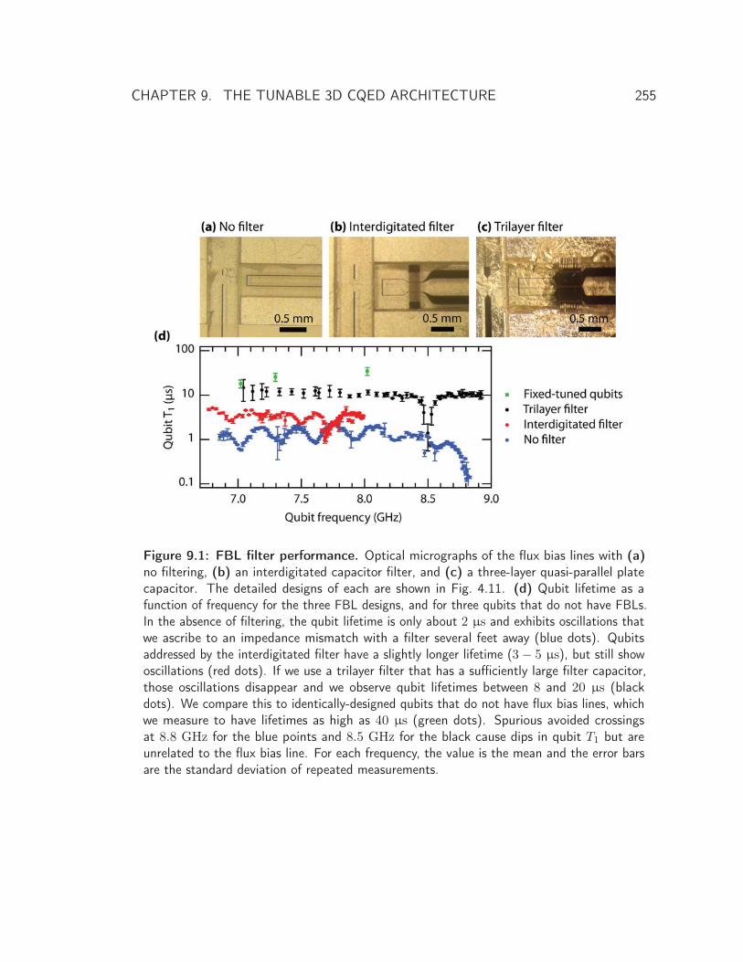
CHAPTER 9. THE TUNABLE 3D CQED ARCHITECTURE 255
Figure 9.1: FBL filter performance. Optical micrographs of the flux bias lines with (a)no filtering, (b) an interdigitated capacitor filter, and (c) a three-layer quasi-parallel platecapacitor. The detailed designs of each are shown in Fig. 4.11. (d) Qubit lifetime as afunction of frequency for the three FBL designs, and for three qubits that do not have FBLs.In the absence of filtering, the qubit lifetime is only about 2 μs and exhibits oscillations thatwe ascribe to an impedance mismatch with a filter several feet away (blue dots). Qubitsaddressed by the interdigitated filter have a slightly longer lifetime (3 − 5 μs), but still showoscillations (red dots). If we use a trilayer filter that has a sufficiently large filter capacitor,those oscillations disappear and we observe qubit lifetimes between 8 and 20 μs (blackdots). We compare this to identically-designed qubits that do not have flux bias lines, whichwe measure to have lifetimes as high as 40 μs (green dots). Spurious avoided crossingsat 8.8 GHz for the blue points and 8.5 GHz for the black cause dips in qubit T1 but areunrelated to the flux bias line. For each frequency, the value is the mean and the error barsare the standard deviation of repeated measurements.
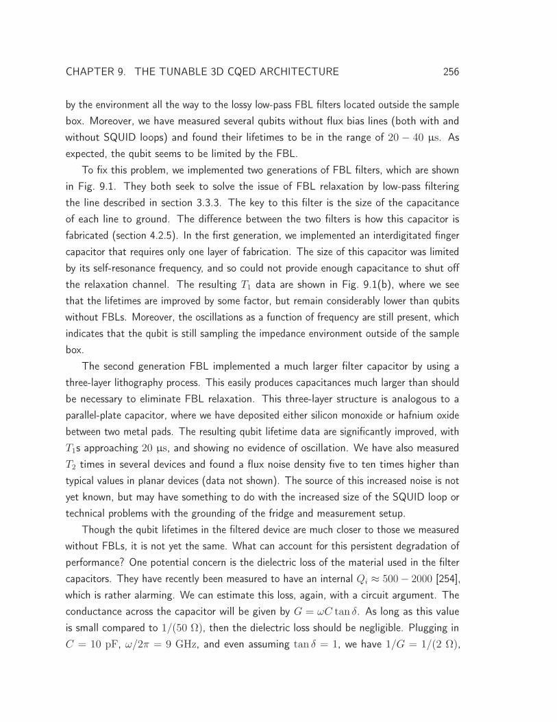
CHAPTER 9. THE TUNABLE 3D CQED ARCHITECTURE 256
by the environment all the way to the lossy low-pass FBL filters located outside the samplebox. Moreover, we have measured several qubits without flux bias lines (both with andwithout SQUID loops) and found their lifetimes to be in the range of 20 − 40 μs. Asexpected, the qubit seems to be limited by the FBL.
To fix this problem, we implemented two generations of FBL filters, which are shownin Fig. 9.1. They both seek to solve the issue of FBL relaxation by low-pass filteringthe line described in section 3.3.3. The key to this filter is the size of the capacitanceof each line to ground. The difference between the two filters is how this capacitor isfabricated (section 4.2.5). In the first generation, we implemented an interdigitated fingercapacitor that requires only one layer of fabrication. The size of this capacitor was limitedby its self-resonance frequency, and so could not provide enough capacitance to shut offthe relaxation channel. The resulting T1 data are shown in Fig. 9.1(b), where we seethat the lifetimes are improved by some factor, but remain considerably lower than qubitswithout FBLs. Moreover, the oscillations as a function of frequency are still present, whichindicates that the qubit is still sampling the impedance environment outside of the samplebox.
The second generation FBL implemented a much larger filter capacitor by using athree-layer lithography process. This easily produces capacitances much larger than shouldbe necessary to eliminate FBL relaxation. This three-layer structure is analogous to aparallel-plate capacitor, where we have deposited either silicon monoxide or hafnium oxidebetween two metal pads. The resulting qubit lifetime data are significantly improved, withT1s approaching 20 μs, and showing no evidence of oscillation. We have also measuredT2 times in several devices and found a flux noise density five to ten times higher thantypical values in planar devices (data not shown). The source of this increased noise is notyet known, but may have something to do with the increased size of the SQUID loop ortechnical problems with the grounding of the fridge and measurement setup.
Though the qubit lifetimes in the filtered device are much closer to those we measuredwithout FBLs, it is not yet the same. What can account for this persistent degradation ofperformance? One potential concern is the dielectric loss of the material used in the filtercapacitors. They have recently been measured to have an internal Qi ≈ 500− 2000 [254],which is rather alarming. We can estimate this loss, again, with a circuit argument. Theconductance across the capacitor will be given by G = ωC tan δ. As long as this valueis small compared to 1/(50 Ω), then the dielectric loss should be negligible. Plugging inC = 10 pF, ω/2π = 9 GHz, and even assuming tan δ = 1, we have 1/G = 1/(2 Ω),
CHAPTER 9. THE TUNABLE 3D CQED ARCHITECTURE 257
160
120
80
40
0
Tim
e (n
s)
8.708.658.608.558.50Spec frequency (GHz)
6.5
6.0
5.5
5.0
4.5
Volta
ge (m
V)
16012080400Time (ns)
7.5
7.0
6.5
6.0
5.5
5.0
4.5
8.5370 GHz 8.6565 GHz
Measure
Qub
it p
ulse Flux pulse(a)
(b) (c)
Figure 9.2: Fast flux characterization with flux spectroscopy. (a) To perform fluxspectroscopy, we suddenly detune the qubit from its starting position with a square flux pulse,depicted in blue. After holding for some time, the qubit is returned to its home position andmeasured. During this time, we apply a gaussian spectroscopy pulse at some frequency anddelay relative to the flux pulse. Here, the width of that gaussian is σ = 20 ns and its totalduration is 4σ. (b) The ensemble-averaged measurement is plotted as a function of the delayand frequency of the spectroscopy pulse. We see features for small times at 8.537 GHz andfor large times at 8.657 GHz, indicating that the qubit initially starts at the first frequencybut jumps to the second upon the application of the flux pulse. (c) Taking cuts along the tworelevant frequencies, we see that these features are rounded in time. The rounding is due tothe temporal extent of the gaussian pulses. Fitting them to error functions, we find that theoffset between the centers of the two curves is only a few nanoseconds. This indicates thatthe qubit is moving between the two positions in that time. Note that the two y-scales aredifferent for the two plots because the spectroscopy pulse drives a slightly different rotationat the two frequencies because of the cavity filtering.
indicating that the dielectric loss of this capacitor is irrelevant. This treatment does notaccount for direct hybridization of the qubit mode with this dielectric, however. If thequbit stores as little as 0.1% of its energy there, it could constitute the dominant sourceof relaxation. Whether or not this is a prominent effect remains an open question as ofthe writing of this thesis.
CHAPTER 9. THE TUNABLE 3D CQED ARCHITECTURE 258
9.1.1 Fast flux performance
The addition of the low-pass filter to the flux bias line potentially slows down its responsetime. The characteristic frequency of the filter is set by the size of the capacitor, whichwe aim to control with lithography. What if we accidentally make a much larger capacitorthan we intend? Evidence would not appear in the T1 data nor in the static flux tuning; itwould only become apparent in a slowing of the rise time of an applied flux pulse. We candirectly measure this time with flux spectroscopy. As shown in the cartoon of Fig. 9.2(a),we perform pulsed spectroscopy simultaneous with a flux pulse. Some fixed time after theexperiment begins, we move the qubit from its home position to another frequency as fastas possible with a square flux pulse. We wait there for a few microseconds, flux back, andmeasure the qubit. During this time, we apply a gaussian π pulse of some frequency atsome delay relative to the flux pulse. We then ensemble average as a function of bothpulse frequency and delay.
The result of this experiment is shown in Fig. 9.2(b). We see that the qubit initiallystarts at 8.537 GHz and, at t ≈ 50 ns, jumps to a frequency of 8.657 GHz. We take cutsalong both frequencies and plot them, shown in (b). The observed rounding is due to thetemporal width of the qubit spectroscopy pulse used to interrogate the system. To seethis, suppose that the qubit moves suddenly away during the application of the pulse, attf . If its final position is far detuned from the spectroscopy frequency, the rotation thatthe qubit experiences will be given by the integral of the pulse from t = 0 to tf . Since thepulse is gaussian and the rotation angle is given by the integral of the applied amplitude,the rotation angle is specified by the integral of that gaussian: an error function. Wefit both sets of data to that function with time constants of t = 20 ns. The differencebetween the centers of the two fits gives the transit time of the qubit, here being 5 ns.
This experiment is a bit unusual in that it aims to be sensitive to both frequency andtime. Since we use relatively long 20 ns pulses in Fig. 9.2(b), the data is relatively smoothin time and spectrally narrow. However, as we show in Fig. 9.3, by using faster 5 ns
pulses, we substantially broaden the qubit response. This increases our temporal resolution,revealing fast ringing of the qubit frequency once it has neared its final frequency. Asdescribed in section 7.1.1, this ringing is due to the response function of the TektronixAWG and the flux line itself, and can be mitigated with linear deconvolution.

CHAPTER 9. THE TUNABLE 3D CQED ARCHITECTURE 259
160
120
80
40
0Ti
me
(ns)
8.708.658.608.558.50Spec frequency (GHz)
Figure 9.3: Flux spectroscopy with 5 ns gaussian pulse width. We repeat the experi-ment shown in Fig. 9.2 with 5 ns gaussian pulses instead of 20 ns. The spectral width ofthe qubit response is significantly broadened, but the temporal resolution is commensuratelyhigher. As a result, we can resolve ringing of the qubit frequency once it reaches its finalfrequency. These dynamics can be mitigated with linear deconvolution (section 7.1.1).
9.2 Device characterization with Fock states
Since our flux bias line filtering is working as desired, we now turn our attention toperforming experiments with a particular device. This section reports on a single-cavity3D device with a single trilayer-filtered tunable qubit. The Hamiltonian of this system iswell-approximated by
H/� = ωq b†b − α
2b†b†bb+ ωca
†a − K
2a†a†aa − χa†ab†b, (9.1)
where b†/b are the qubit raising and lowering operators, a†/a are the cavity raising andlowering operators, α is the qubit anharmonicity, K is the cavity anharmonicity (alsoknown as the self-Kerr term), and χ is the state-dependent dispersive shift [138, 255]. Inthis treatment, the cavity and qubit are governed by the same dynamics, differentiatedonly by the magnitude of α and K. Note that this is a slightly different definition ofχ than the one used in previous chapters. Here we adopt the more modern conventionwhere number split peaks are separated by χ [107, 138]. In previous chapters, includingsection 3.2.3, we had defined that separation to be 2χ.
The qubit in this device has a maximum frequency that is very close to vacuum-Rabi.The cavity therefore inherits enough K anharmonicity that we can directly pulse it to create
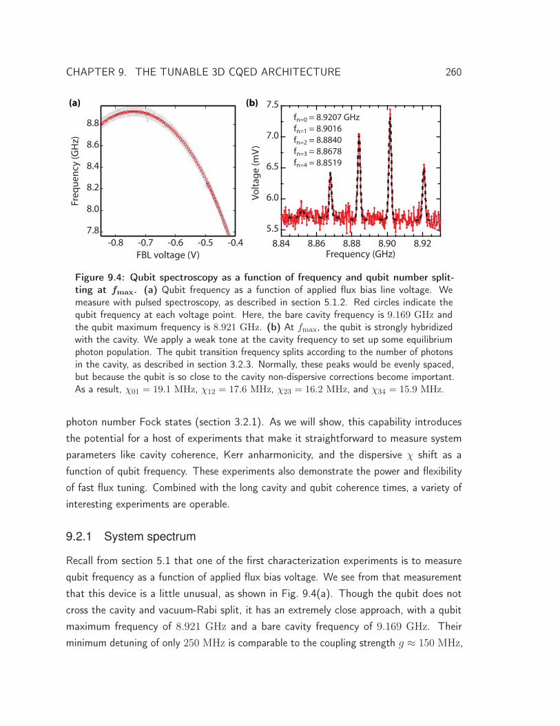
CHAPTER 9. THE TUNABLE 3D CQED ARCHITECTURE 260
7.5
7.0
6.5
6.0
5.5
Volta
ge (m
V)
8.928.908.888.868.84Frequency (GHz)
fn=0 = 8.9207 GHzfn=1 = 8.9016fn=2 = 8.8840fn=3 = 8.8678fn=4 = 8.8519
8.8
8.6
8.4
8.2
8.0
7.8
Freq
uenc
y (G
Hz)
-0.8 -0.7 -0.6 -0.5 -0.4FBL voltage (V)
(a) (b)
Figure 9.4: Qubit spectroscopy as a function of frequency and qubit number split-ting at fmax. (a) Qubit frequency as a function of applied flux bias line voltage. Wemeasure with pulsed spectroscopy, as described in section 5.1.2. Red circles indicate thequbit frequency at each voltage point. Here, the bare cavity frequency is 9.169 GHz andthe qubit maximum frequency is 8.921 GHz. (b) At fmax, the qubit is strongly hybridizedwith the cavity. We apply a weak tone at the cavity frequency to set up some equilibriumphoton population. The qubit transition frequency splits according to the number of photonsin the cavity, as described in section 3.2.3. Normally, these peaks would be evenly spaced,but because the qubit is so close to the cavity non-dispersive corrections become important.As a result, χ01 = 19.1 MHz, χ12 = 17.6 MHz, χ23 = 16.2 MHz, and χ34 = 15.9 MHz.
photon number Fock states (section 3.2.1). As we will show, this capability introducesthe potential for a host of experiments that make it straightforward to measure systemparameters like cavity coherence, Kerr anharmonicity, and the dispersive χ shift as afunction of qubit frequency. These experiments also demonstrate the power and flexibilityof fast flux tuning. Combined with the long cavity and qubit coherence times, a variety ofinteresting experiments are operable.
9.2.1 System spectrum
Recall from section 5.1 that one of the first characterization experiments is to measurequbit frequency as a function of applied flux bias voltage. We see from that measurementthat this device is a little unusual, as shown in Fig. 9.4(a). Though the qubit does notcross the cavity and vacuum-Rabi split, it has an extremely close approach, with a qubitmaximum frequency of 8.921 GHz and a bare cavity frequency of 9.169 GHz. Theirminimum detuning of only 250 MHz is comparable to the coupling strength g ≈ 150 MHz,

CHAPTER 9. THE TUNABLE 3D CQED ARCHITECTURE 261
11.0
10.0
9.0
8.0
Volta
ge (m
V)
9.19609.19569.19529.1948Frequency (GHz)
f01 = 9.1956 GHzf02/2 = 9.1951 GHz
Cav. sat. tone
0-photon pulse
2nd mode msm’t
(a)
(b)
Figure 9.5: Pulsed spectroscopy of anharmonic cavity. (a) In order to measure thespectrum of the cavity, we must slightly modify our conventional pulsed spectroscopy sequence.We begin with a long cavity saturation tone, as with normal spectroscopy. In order to besensitive to the resulting cavity state, we map its population onto the qubit by applyinga π pulse on the 0-photon number-split peak at 8.9207 GHz. To detect the state of thequbit, we measure with the second spatial mode of the cavity at 11.244 GHz. We do thisto avoid our qubit measurement contrast being sensitive to the number of photons storedin the first mode. The qubit is also strongly coupled to the second mode because it isphysically offset from the center of the cavity, a symmetry point usually used to eliminate thecoupling strength. We will continue using this trick to measure the cavity state throughoutthis chapter. (b) The resulting cavity spectrum reveals resolved f01 and f02/2 transitions,just as we see with a strongly-driven qubit (section 5.1.2). This indicates that the cavity hasinherited an anharmonicity of about 1 MHz due to its hybridization with the qubit. Notethat the y-axis is inverted because we get a large voltage when the qubit pulse conditional onzero photons succeeds. When our spectroscopy tone is in resonance with a cavity transition,we populate the cavity, causing the qubit pulse to fail and giving us a dip in measurementvoltage.
making the qubit strongly non-dispersive at fmax. This fact is illustrated clearly whenwe measure qubit number splitting, shown in Fig. 9.4(b). As described in section 3.2.3,normal number-split peaks are evenly spaced by χ. However, here the splitting is not evenlyspaced, with, for example, the difference between the qubit transition frequency with 0and 1 photons of 19.1 MHz, but only 17.6 MHz between 1 and 2 photons. This is anindication that the qubit and cavity are so strongly hybridized at fmax that the dispersiveapproximation has broken down.

CHAPTER 9. THE TUNABLE 3D CQED ARCHITECTURE 262
We observe another indication of this non-dispersive behavior in the spectrum ofthe cavity with the qubit at its maximum frequency. The procedure to perform cavityspectroscopy is shown in Fig. 9.5(a), where we make use of qubit number splitting aswell as the fact that the qubit couples to more than one spatial mode of the cavity. Theresulting data are shown in (b), demonstrating that we can resolve the individual f01and f02/2 transitions. The cavity is so strongly hybridized with the qubit that it inheritsappreciable anharmonicity; in essence, the cavity behaves like a transmon qubit. At fmax,this anharmonicity is approximately 1 MHz, which is substantially larger than the cavitylinewidth. This is known as a Kerr nonlinearity, and, as we will see in section 9.3, it hasinteresting consequences for the dynamics of the cavity [107, 167, 256].
9.2.2 Cavity Rabi oscillation
The substantial anharmonicity of the cavity makes it possible to directly populate Focknumber states. Just as with a qubit, we apply a gaussian pulse to the cavity resonancefrequency that is sufficiently spectrally narrow to address only the desired transition. Thedifference here is that the anharmonicity is so small that we must use extremely slowpulses, here a gaussian σ = 1 μs. The procedure to do a Rabi oscillation on the cavity isshown in Fig. 9.6(a). After this slow gaussian pulse, we again map the resulting cavitystate to the qubit by performing a π pulse on the 0-photon peak and measuring its statewith the second cavity mode, done previously with cavity spectroscopy. As shown in (b),we can extend this procedure by applying a rotation on the 1-2 transition of the cavity aswell. The resulting oscillations shown in (c) are consistent with our expectations, with the1-2 oscillation sped up by
√2 and its amplitude reduced due to the longer pulse sequence
length.
9.2.3 Cavity lifetime
The ability to create single Fock states in the cavity is extremely useful for characterizingits properties. The simplest example experiment is to measure the cavity lifetime. Dueto cavity anharmonicity and the glassy physics that sometimes dominates its loss, theapparent lifetime of the cavity can be a strong function of the magnitude of its excitation[156]. Since we are normally interested in the low-power lifetime, we can only displace withan extremely weak tone that populates at most ∼ 1 photon. We can then either watch thisenergy leak out in the time domain or measure the cavity spectral width in the frequency
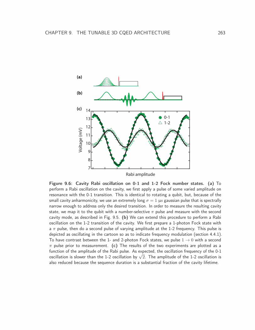
CHAPTER 9. THE TUNABLE 3D CQED ARCHITECTURE 263
14
13
12
11
10
9
8
7
Volta
ge (m
V)
Rabi amplitude
0-1 1-2
(a)
(b)
(c)
Figure 9.6: Cavity Rabi oscillation on 0-1 and 1-2 Fock number states. (a) Toperform a Rabi oscillation on the cavity, we first apply a pulse of some varied amplitude onresonance with the 0-1 transition. This is identical to rotating a qubit, but, because of thesmall cavity anharmonicity, we use an extremely long σ = 1 μs gaussian pulse that is spectrallynarrow enough to address only the desired transition. In order to measure the resulting cavitystate, we map it to the qubit with a number-selective π pulse and measure with the secondcavity mode, as described in Fig. 9.5. (b) We can extend this procedure to perform a Rabioscillation on the 1-2 transition of the cavity. We first prepare a 1-photon Fock state witha π pulse, then do a second pulse of varying amplitude at the 1-2 frequency. This pulse isdepicted as oscillating in the cartoon so as to indicate frequency modulation (section 4.4.1).To have contrast between the 1- and 2-photon Fock states, we pulse 1 → 0 with a secondπ pulse prior to measurement. (c) The results of the two experiments are plotted as afunction of the amplitude of the Rabi pulse. As expected, the oscillation frequency of the 0-1oscillation is slower than the 1-2 oscillation by
√2. The amplitude of the 1-2 oscillation is
also reduced because the sequence duration is a substantial fraction of the cavity lifetime.

CHAPTER 9. THE TUNABLE 3D CQED ARCHITECTURE 264
3.0
2.5
2.0
1.5
Volta
ge (m
V)
100806040200Delay time (μs)
Cavity T1 = 31.4 ± 0.8 μs
(a)
(b)
Figure 9.7: Cavity T1 measured with Fock state. (a) To measure the cavity lifetime,we first prepare a 1-photon Fock state with a π pulse on the cavity and wait for some amountof time. We then measure the resulting cavity state with a number-selective π pulse andsecond-mode measurement, as before. (b) We plot the average remaining cavity populationas a function of the delay time. The cavity lifetime is found to be 31.4 ± 0.8 μs with thequbit at fmax.
domain with transmission. (The second tactic actually measures some combination of T1
and T2.) Both approaches suffer from a low SNR since the signal we are looking for isvery small. It can also be difficult to ascertain that you are driving with a small enoughpower. A superior method for measuring cavity lifetime is shown in Fig. 9.7(a). There, wereplicate the normal sequence for measuring qubit T1 by applying a π pulse to the cavitywith our slow gaussian and delaying for a variable length of time prior to measurement.As before, we measure by mapping the cavity state to the qubit with a number-selective π
pulse. The result is shown in (b), where we find a cavity lifetime of about 30 μs when thequbit is at its maximum frequency.
We can extend this protocol to measure the cavity lifetime as its hybridization withthe qubit is turned off. If the qubit is lossier than the cavity, the dispersive couplingmay limit the cavity’s lifetime. The procedure is shown in Fig. 9.8(a). The sequence isidentical to the one described in Fig. 9.7, except that during the waiting time, the qubitis moved away to some other detuning with a flux pulse. In Fig. 9.8(b), we show theresulting measurement when the flux pulse amplitude is chosen to move the qubit near itsminimum frequency, estimated to be 2− 3 GHz. The cavity lifetime is found to be 40 μs,
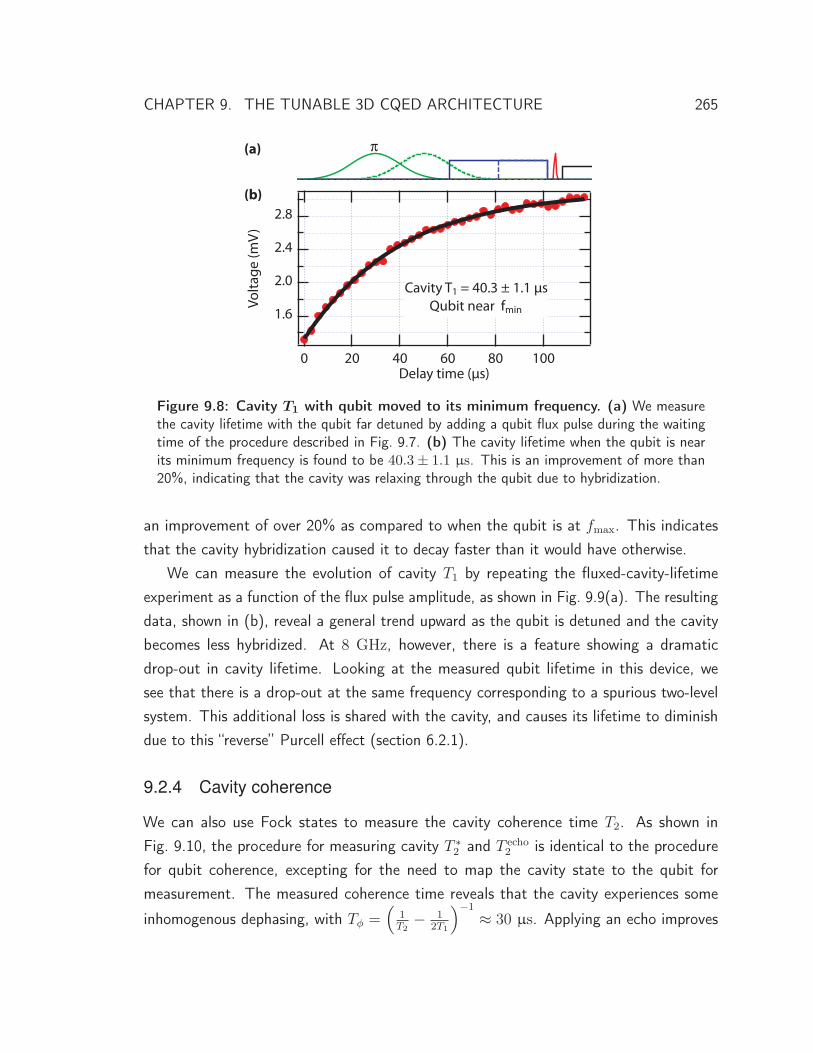
CHAPTER 9. THE TUNABLE 3D CQED ARCHITECTURE 265
2.8
2.4
2.0
1.6
Volta
ge (m
V)
100806040200Delay time (μs)
Cavity T1 = 40.3 ± 1.1 μs Qubit near fmin
(a)
(b)
Figure 9.8: Cavity T1 with qubit moved to its minimum frequency. (a) We measurethe cavity lifetime with the qubit far detuned by adding a qubit flux pulse during the waitingtime of the procedure described in Fig. 9.7. (b) The cavity lifetime when the qubit is nearits minimum frequency is found to be 40.3± 1.1 μs. This is an improvement of more than20%, indicating that the cavity was relaxing through the qubit due to hybridization.
an improvement of over 20% as compared to when the qubit is at fmax. This indicatesthat the cavity hybridization caused it to decay faster than it would have otherwise.
We can measure the evolution of cavity T1 by repeating the fluxed-cavity-lifetimeexperiment as a function of the flux pulse amplitude, as shown in Fig. 9.9(a). The resultingdata, shown in (b), reveal a general trend upward as the qubit is detuned and the cavitybecomes less hybridized. At 8 GHz, however, there is a feature showing a dramaticdrop-out in cavity lifetime. Looking at the measured qubit lifetime in this device, wesee that there is a drop-out at the same frequency corresponding to a spurious two-levelsystem. This additional loss is shared with the cavity, and causes its lifetime to diminishdue to this “reverse” Purcell effect (section 6.2.1).
9.2.4 Cavity coherence
We can also use Fock states to measure the cavity coherence time T2. As shown inFig. 9.10, the procedure for measuring cavity T ∗
2 and T echo2 is identical to the procedure
for qubit coherence, excepting for the need to map the cavity state to the qubit formeasurement. The measured coherence time reveals that the cavity experiences some
inhomogenous dephasing, with Tφ =(
1T2
− 12T1
)−1
≈ 30 μs. Applying an echo improves
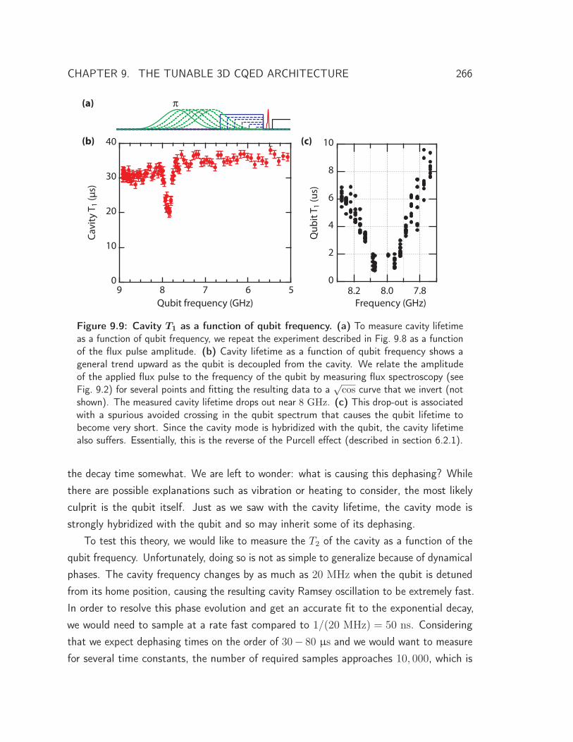
CHAPTER 9. THE TUNABLE 3D CQED ARCHITECTURE 266
40
30
20
10
0
Cavi
ty T
1 (μs
)
9 8 7 6 5Qubit frequency (GHz)
10
8
6
4
2
0
Qub
it T 1
(us)
8.2 8.0 7.8Frequency (GHz)
(a)
(b) (c)
Figure 9.9: Cavity T1 as a function of qubit frequency. (a) To measure cavity lifetimeas a function of qubit frequency, we repeat the experiment described in Fig. 9.8 as a functionof the flux pulse amplitude. (b) Cavity lifetime as a function of qubit frequency shows ageneral trend upward as the qubit is decoupled from the cavity. We relate the amplitudeof the applied flux pulse to the frequency of the qubit by measuring flux spectroscopy (seeFig. 9.2) for several points and fitting the resulting data to a
√cos curve that we invert (not
shown). The measured cavity lifetime drops out near 8 GHz. (c) This drop-out is associatedwith a spurious avoided crossing in the qubit spectrum that causes the qubit lifetime tobecome very short. Since the cavity mode is hybridized with the qubit, the cavity lifetimealso suffers. Essentially, this is the reverse of the Purcell effect (described in section 6.2.1).
the decay time somewhat. We are left to wonder: what is causing this dephasing? Whilethere are possible explanations such as vibration or heating to consider, the most likelyculprit is the qubit itself. Just as we saw with the cavity lifetime, the cavity mode isstrongly hybridized with the qubit and so may inherit some of its dephasing.
To test this theory, we would like to measure the T2 of the cavity as a function of thequbit frequency. Unfortunately, doing so is not as simple to generalize because of dynamicalphases. The cavity frequency changes by as much as 20 MHz when the qubit is detunedfrom its home position, causing the resulting cavity Ramsey oscillation to be extremely fast.In order to resolve this phase evolution and get an accurate fit to the exponential decay,we would need to sample at a rate fast compared to 1/(20 MHz) = 50 ns. Consideringthat we expect dephasing times on the order of 30− 80 μs and we would want to measurefor several time constants, the number of required samples approaches 10, 000, which is

CHAPTER 9. THE TUNABLE 3D CQED ARCHITECTURE 267
(a) (b)
12
11
10
9
8
Volta
ge (m
V)
3020100Delay time (μs)
Cav T2* = 21.3 ± 1.2 μs
12080400Delay time (μs)
Cav T2echo = 30.6 ± 1.2 μs
/2 /2 /2 /2
Figure 9.10: Cavity T ∗2 and T echo
2 . (a) The cavity coherence time T ∗2 is measured in the
same way as with a qubit. We prepare a superposition of 0 and 1 photons by applying a π/2pulse to the cavity. We then delay for some period of time before applying a second π/2pulse and measure by mapping the cavity state to the qubit with a number-selective qubitrotation. The cavity pulses are slightly detuned so as to see an oscillation. The resultingdephasing time is found to be 21.3 ± 1.2 μs, with the uncertainty given by the fit. Thiscorresponds to a pure dephasing time of approximately 30 μs. (b) We can also perform aHahn echo experiment with the addition of a π pulse on the cavity exactly half way throughthe experiment. The dephasing time increases to 30.6± 1.2 μs. Here, we sweep the angle ofthe final π/2 pulse to see an oscillation, though that fact is not indicated in the cartoon forclarity.
quite unfeasible. Alternatively, we can use the method shown in Fig. 9.11(a). There, wechoose several fixed times and repeat the Ramsey experiment for each while sweepingthe angle of the final π/2 pulse. At each time we get a sinusoid with a phase that, fromour point of view, is random. The amplitude of this oscillation tells us the amount ofphase coherence remaining at that time. As shown in (b), we can plot the amplitudes foreach time and fit them to an exponential decay. We see that when we have detuned thequbit by about 2 GHz, the cavity coherence time has improved to more than 60 μs. This
corresponds to a pure dephasing time of Tφ =(
160 μs
− 12·35 μs
)−1
≈ 400 μs. Clearly, theinherited dephasing from the qubit was dominating the cavity coherence.
As before, we can reveal the evolution of this decoupling by measuring T2 as a functionof qubit frequency. As shown in Fig. 9.12, this is done by repeating the procedure fromFig. 9.11 for a variety of flux pulse amplitudes. The resulting data show two general trends.At first, as we detune the qubit from its maximum frequency, the cavity coherence time is
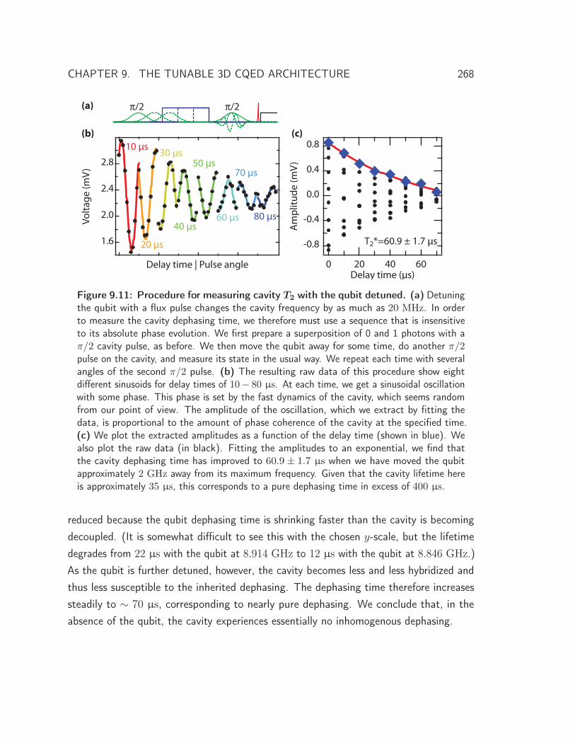
CHAPTER 9. THE TUNABLE 3D CQED ARCHITECTURE 268
2.8
2.4
2.0
1.6
Volta
ge (m
V)
Delay time | Pulse angle
10 μs
20 μs
30 μs
40 μs
50 μs
60 μs
70 μs
80 μs
-0.8
-0.4
0.0
0.4
0.8
Am
plitu
de (m
V)
6040200Delay time (μs)
T2*=60.9 ± 1.7 μs
(a)
(c)(b)
/2 /2
Figure 9.11: Procedure for measuring cavity T2 with the qubit detuned. (a) Detuningthe qubit with a flux pulse changes the cavity frequency by as much as 20 MHz. In orderto measure the cavity dephasing time, we therefore must use a sequence that is insensitiveto its absolute phase evolution. We first prepare a superposition of 0 and 1 photons with aπ/2 cavity pulse, as before. We then move the qubit away for some time, do another π/2pulse on the cavity, and measure its state in the usual way. We repeat each time with severalangles of the second π/2 pulse. (b) The resulting raw data of this procedure show eightdifferent sinusoids for delay times of 10− 80 μs. At each time, we get a sinusoidal oscillationwith some phase. This phase is set by the fast dynamics of the cavity, which seems randomfrom our point of view. The amplitude of the oscillation, which we extract by fitting thedata, is proportional to the amount of phase coherence of the cavity at the specified time.(c) We plot the extracted amplitudes as a function of the delay time (shown in blue). Wealso plot the raw data (in black). Fitting the amplitudes to an exponential, we find thatthe cavity dephasing time has improved to 60.9 ± 1.7 μs when we have moved the qubitapproximately 2 GHz away from its maximum frequency. Given that the cavity lifetime hereis approximately 35 μs, this corresponds to a pure dephasing time in excess of 400 μs.
reduced because the qubit dephasing time is shrinking faster than the cavity is becomingdecoupled. (It is somewhat difficult to see this with the chosen y-scale, but the lifetimedegrades from 22 μs with the qubit at 8.914 GHz to 12 μs with the qubit at 8.846 GHz.)As the qubit is further detuned, however, the cavity becomes less and less hybridized andthus less susceptible to the inherited dephasing. The dephasing time therefore increasessteadily to ∼ 70 μs, corresponding to nearly pure dephasing. We conclude that, in theabsence of the qubit, the cavity experiences essentially no inhomogenous dephasing.

CHAPTER 9. THE TUNABLE 3D CQED ARCHITECTURE 269
/2 /2
100
80
60
40
20
0
Tim
e (μ
s)
9 8 7Qubit frequency (GHz)
T1
T2*
Figure 9.12: Cavity T1 and T2 as a function of qubit frequency. We perform theexperiment described in Fig. 9.11 as a function of qubit frequency by varying the amplitudeof the qubit flux pulse. We plot the measured cavity dephasing time, revealing that itinitially decreases as the qubit lifetime rapidly degrades away from fmax. When the qubit is at8.914 GHz, the cavity T2 is 22 μs, but reduces to only 12 μs with the qubit at 8.846 GHz. Forlarger detunings, however, the dephasing time increases as the cavity becomes less hybridizedand therefore becomes less susceptible to qubit dephasing. Error bars are the standarddeviation of several repeated measurements. Uncertainties are larger for big detuningsbecause we are unable to measure for larger delay times than 80 μs due to the memorylimitations of our AWG. Therefore, we do not sample far on the exponential curve when thecavity coherence time gets long. As before, we relate the applied flux pulse amplitude toqubit frequency with flux spectroscopy. We also plot the previously-measured cavity T1 forcomparison, which shows that the cavity approaches T2 = 2T1 for large detunings.
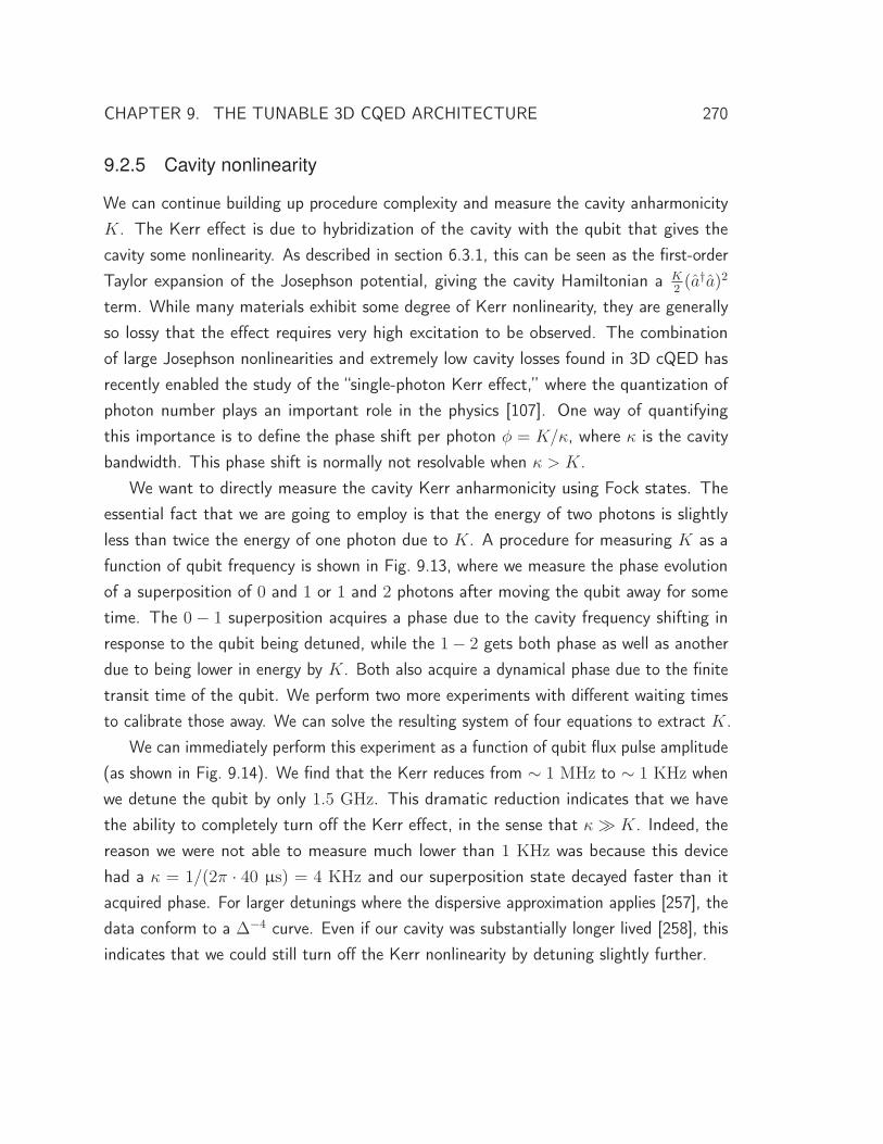
CHAPTER 9. THE TUNABLE 3D CQED ARCHITECTURE 270
9.2.5 Cavity nonlinearity
We can continue building up procedure complexity and measure the cavity anharmonicityK. The Kerr effect is due to hybridization of the cavity with the qubit that gives thecavity some nonlinearity. As described in section 6.3.1, this can be seen as the first-orderTaylor expansion of the Josephson potential, giving the cavity Hamiltonian a K
2(a†a)2
term. While many materials exhibit some degree of Kerr nonlinearity, they are generallyso lossy that the effect requires very high excitation to be observed. The combinationof large Josephson nonlinearities and extremely low cavity losses found in 3D cQED hasrecently enabled the study of the “single-photon Kerr effect,” where the quantization ofphoton number plays an important role in the physics [107]. One way of quantifyingthis importance is to define the phase shift per photon φ = K/κ, where κ is the cavitybandwidth. This phase shift is normally not resolvable when κ > K.
We want to directly measure the cavity Kerr anharmonicity using Fock states. Theessential fact that we are going to employ is that the energy of two photons is slightlyless than twice the energy of one photon due to K. A procedure for measuring K as afunction of qubit frequency is shown in Fig. 9.13, where we measure the phase evolutionof a superposition of 0 and 1 or 1 and 2 photons after moving the qubit away for sometime. The 0 − 1 superposition acquires a phase due to the cavity frequency shifting inresponse to the qubit being detuned, while the 1− 2 gets both phase as well as anotherdue to being lower in energy by K. Both also acquire a dynamical phase due to the finitetransit time of the qubit. We perform two more experiments with different waiting timesto calibrate those away. We can solve the resulting system of four equations to extract K.
We can immediately perform this experiment as a function of qubit flux pulse amplitude(as shown in Fig. 9.14). We find that the Kerr reduces from ∼ 1 MHz to ∼ 1 KHz whenwe detune the qubit by only 1.5 GHz. This dramatic reduction indicates that we havethe ability to completely turn off the Kerr effect, in the sense that κ � K. Indeed, thereason we were not able to measure much lower than 1 KHz was because this devicehad a κ = 1/(2π · 40 μs) = 4 KHz and our superposition state decayed faster than itacquired phase. For larger detunings where the dispersive approximation applies [257], thedata conform to a Δ−4 curve. Even if our cavity was substantially longer lived [258], thisindicates that we could still turn off the Kerr nonlinearity by detuning slightly further.
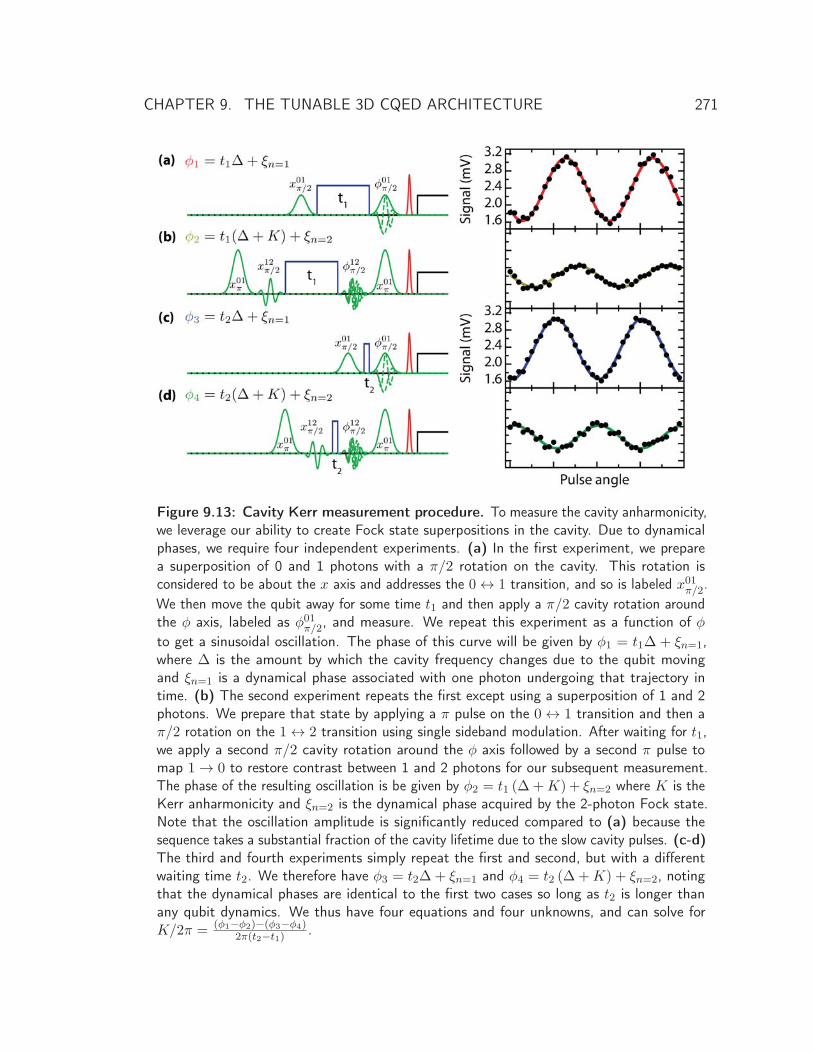
CHAPTER 9. THE TUNABLE 3D CQED ARCHITECTURE 271
Figure 9.13: Cavity Kerr measurement procedure. To measure the cavity anharmonicity,we leverage our ability to create Fock state superpositions in the cavity. Due to dynamicalphases, we require four independent experiments. (a) In the first experiment, we preparea superposition of 0 and 1 photons with a π/2 rotation on the cavity. This rotation isconsidered to be about the x axis and addresses the 0 ↔ 1 transition, and so is labeled x01π/2.We then move the qubit away for some time t1 and then apply a π/2 cavity rotation aroundthe φ axis, labeled as φ01
π/2, and measure. We repeat this experiment as a function of φto get a sinusoidal oscillation. The phase of this curve will be given by φ1 = t1Δ+ ξn=1,where Δ is the amount by which the cavity frequency changes due to the qubit movingand ξn=1 is a dynamical phase associated with one photon undergoing that trajectory intime. (b) The second experiment repeats the first except using a superposition of 1 and 2photons. We prepare that state by applying a π pulse on the 0 ↔ 1 transition and then aπ/2 rotation on the 1 ↔ 2 transition using single sideband modulation. After waiting for t1,we apply a second π/2 cavity rotation around the φ axis followed by a second π pulse tomap 1 → 0 to restore contrast between 1 and 2 photons for our subsequent measurement.The phase of the resulting oscillation is be given by φ2 = t1 (Δ +K) + ξn=2 where K is theKerr anharmonicity and ξn=2 is the dynamical phase acquired by the 2-photon Fock state.Note that the oscillation amplitude is significantly reduced compared to (a) because thesequence takes a substantial fraction of the cavity lifetime due to the slow cavity pulses. (c-d)The third and fourth experiments simply repeat the first and second, but with a differentwaiting time t2. We therefore have φ3 = t2Δ+ ξn=1 and φ4 = t2 (Δ +K) + ξn=2, notingthat the dynamical phases are identical to the first two cases so long as t2 is longer thanany qubit dynamics. We thus have four equations and four unknowns, and can solve forK/2π = (φ1−φ2)−(φ3−φ4)
2π(t2−t1).

CHAPTER 9. THE TUNABLE 3D CQED ARCHITECTURE 272
0.0012
46
0.012
46
0.12
46
1Ca
vity
Ker
r / 2
(MH
z)
9.0 8.5 8.0 7.5Qubit frequency (GHz)
Figure 9.14: Cavity Kerr as a function of qubit frequency. We perform the experimentdescribed in Fig. 9.13 as a function of the qubit flux pulse amplitude. As before, we relate theflux amplitude to the resulting qubit frequency with flux spectroscopy. We plot the measuredKerr value as a function of qubit frequency. Note that the y-axis is logarithmic, and that theKerr parameter drops three orders of magnitude when we detune the qubit by only 1.5 GHz.We plot a Δ−4 curve fit to data starting at 8.5 GHz where the dispersive approximationshould hold. The data is well-fit by this power law, indicating that the Kerr effect can bereduced arbitrarily low with further detuning.
9.2.6 Cavity dispersive shift
We can measure the cavity χ-shift as a function of qubit frequency. As described inFig. 9.15, the sequence is quite similar to the one we used to measure the cavity Kerr. Weprepare either 0 or 1 photon, put the qubit on its equator, flux the qubit to the frequencyat which we want to know χ, wait for some time, then move the qubit back home andinterrogate its phase with a Ramsey experiment. Just as was necessary with Kerr, we haveto perform four experiments to cancel out dynamical phases.
This sequence is somewhat more complicated than is necessary. It calls for performingπ/2 pulses on the qubit at a frequency fhome that was distinct from fmax. By choosingfhome to be far from the cavity, the qubit number splitting can be smaller than our qubitpulse bandwidth. That way we can successfully apply a number insensitive π/2 pulseregardless of the number of cavity photons. This requires high-quality flux deconvolution(see section 7.1.1) because we perform a qubit pulse shortly after the qubit has moved downfrom fmax. Operating at fhome is a requirement if, for example, we wanted to interrogate
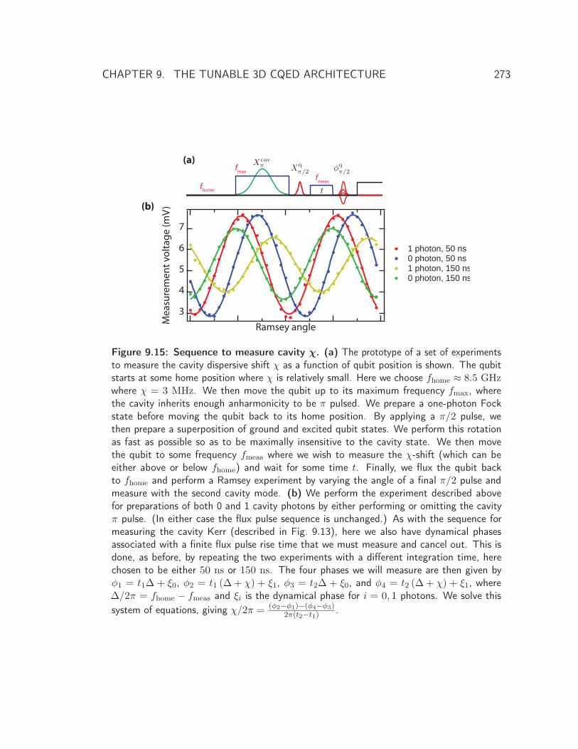
CHAPTER 9. THE TUNABLE 3D CQED ARCHITECTURE 273
7
6
5
4
3
Mea
sure
men
t vol
tage
(mV
)
Ramsey angle
Xcavπ Xq
π/2 φqπ/2
t
1 photon, 50 ns 0 photon, 50 ns 1 photon, 150 ns 0 photon, 150 ns
(a)
(b)
fmax
fhome
fmeas
Figure 9.15: Sequence to measure cavity χ. (a) The prototype of a set of experimentsto measure the cavity dispersive shift χ as a function of qubit position is shown. The qubitstarts at some home position where χ is relatively small. Here we choose fhome ≈ 8.5 GHzwhere χ = 3 MHz. We then move the qubit up to its maximum frequency fmax, wherethe cavity inherits enough anharmonicity to be π pulsed. We prepare a one-photon Fockstate before moving the qubit back to its home position. By applying a π/2 pulse, wethen prepare a superposition of ground and excited qubit states. We perform this rotationas fast as possible so as to be maximally insensitive to the cavity state. We then movethe qubit to some frequency fmeas where we wish to measure the χ-shift (which can beeither above or below fhome) and wait for some time t. Finally, we flux the qubit backto fhome and perform a Ramsey experiment by varying the angle of a final π/2 pulse andmeasure with the second cavity mode. (b) We perform the experiment described abovefor preparations of both 0 and 1 cavity photons by either performing or omitting the cavityπ pulse. (In either case the flux pulse sequence is unchanged.) As with the sequence formeasuring the cavity Kerr (described in Fig. 9.13), here we also have dynamical phasesassociated with a finite flux pulse rise time that we must measure and cancel out. This isdone, as before, by repeating the two experiments with a different integration time, herechosen to be either 50 ns or 150 ns. The four phases we will measure are then given byφ1 = t1Δ + ξ0, φ2 = t1 (Δ + χ) + ξ1, φ3 = t2Δ + ξ0, and φ4 = t2 (Δ + χ) + ξ1, whereΔ/2π = fhome − fmeas and ξi is the dynamical phase for i = 0, 1 photons. We solve thissystem of equations, giving χ/2π = (φ2−φ1)−(φ4−φ3)
2π(t2−t1).
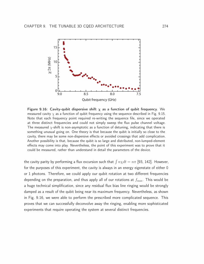
CHAPTER 9. THE TUNABLE 3D CQED ARCHITECTURE 274
15
10
5
0
/2 (M
Hz)
9.0 8.5 8.0 7.5
Qubit frequency (GHz)
Figure 9.16: Cavity-qubit dispersive shift χ as a function of qubit frequency. Wemeasured cavity χ as a function of qubit frequency using the sequence described in Fig. 9.15.Note that each frequency point required re-writing the sequence file, since we operatedat three distinct frequencies and could not simply sweep the flux pulse channel voltage.The measured χ-shift is non-asymptotic as a function of detuning, indicating that there issomething unusual going on. One theory is that because the qubit is initially so close to thecavity, there may be some non-dispersive effects or avoided crossings that add complication.Another possibility is that, because the qubit is so large and distributed, non-lumped-elementeffects may come into play. Nevertheless, the point of this experiment was to prove that itcould be measured, rather than understand in detail the parameters of the device.
the cavity parity by performing a flux excursion such that∫nχdt = nπ [93, 142]. However,
for the purposes of this experiment, the cavity is always in an energy eigenstate of either 0or 1 photons. Therefore, we could apply our qubit rotation at two different frequenciesdepending on the preparation, and thus apply all of our rotations at fmax. This would bea huge technical simplification, since any residual flux bias line ringing would be stronglydamped as a result of the qubit being near its maximum frequency. Nevertheless, as shownin Fig. 9.16, we were able to perform the prescribed more complicated sequence. Thisproves that we can successfully deconvolve away the ringing, enabling more sophisticatedexperiments that require operating the system at several distinct frequencies.
CHAPTER 9. THE TUNABLE 3D CQED ARCHITECTURE 275
9.3 Cavity dynamics
Our lab has recently become interested in using the cavity itself as a quantum resource.Cavities may be longer-lived than even the best 3D qubits [258], have a infinitely-largeHilbert space that can store huge amounts of quantum information [92, 107, 142, 250,259, 260], and suffer from only simple error processes that could potentially be monitoredand reversed in real time [93, 261]. These properties are very attractive for using thecavity as a quantum memory, which may be error correctable [93] and fault-tolerant. Thissection introduces some of the basic building blocks to store and interrogate quantuminformation in a cavity. We measure as an example the Kerr evolution of a coherent statestored in the cavity, and show how we can shut off this evolution using fast flux. As withthe last section, the control and techniques we demonstrate here generalize directly tofuture experiments.
9.3.1 The Husimi Q function
How do we measure the quantum state of a cavity? Since its Hilbert space is infinitelylarge, coming up with an efficient and physically-motivated representation is crucial tomaking good use of this resource. As we saw in section 3.2.1, one possible route is to usethe photon number Fock basis [109]. This is most analogous to how we think of qubitquantum states, but is not a very natural choice for cavities. The canonical cavity state isa “coherent state,” which has a complicated representation in the Fock basis. Since weare likely to use coherent states frequently, it makes sense to use a representation thatacknowledges that fact. We therefore seek to use coherent states as the fundamental basis,rather than Fock states. One consequence of representing our infinite Hilbert space withthose states is that we must now explicitly represent our state using continuous, ratherthan discrete, variables [262, 263]. This reflects the physical reality that two coherentstates always have finite overlap, with 〈α|β〉 = e−|α−β|2 �= δ (α − β).
The simplest “quasiprobability” distribution for representing quantum states of lightis known as the Husimi Q function [264]. It is defined∗ as the modulus squared ofthe resonator state |ψ〉 with a coherent state |α〉, Q(α) = 1
π|〈α|ψ〉|2. The coefficient
1/π is included for normalization, such that∫α∈C Q(α)dα2 = 1. That is, Q(α) is
proportional to the probability that |ψ〉 is the coherent state |α〉. As expected, if ourcavity contains a coherent state |ψ〉 = |β〉, then Q(α) = 1
πe−|α−β|2 . We can also represent
CHAPTER 9. THE TUNABLE 3D CQED ARCHITECTURE 276
Q using the displacement operator D(α) = eαa†−α∗a. Recall from section 3.2.1 that the
displacement operator represents the action of a coherent tone on a harmonic oscillator,and creates coherent states as |α〉 = D(α)|0〉. Using D†(α) = D†(−α), we can writeQ(α) = 1
π|〈0|D(−α)|ψ〉|2.
This expression for Q is highly suggestive of an experimental procedure. To measureQ(α), we could displace the cavity by −α and measure the probability that there are zerophotons using a number-selective qubit π pulse conditioned on n = 0. As before, we usethe first cavity mode as storage for the quantum state and use the second cavity mode tomeasure the qubit. This plan will work, though we must acknowledge a complication ∗.Due to the cross-Kerr effect, there is a direct dispersive coupling between the first andsecond cavity mode. Our second-mode measurement voltage will therefore depend on thenumber of photons in the first cavity mode. This dependence will corrupt our measurementbecause the answer to whether or not the cavity has zero photons should not change if ithas one photon or one hundred. For relatively small displacements at least, the linearity ofthe measurement can be used to compensate for this effect (demonstrated in Fig. 9.17).For each measurement of Q, we measure both with and without the qubit π pulse andsubtract the two measurements, which effectively cancels the cross-Kerr component. Weuse this strategy to measure the Q function of a coherent state in Fig. 9.18.
9.3.2 Kerr evolution
The Q function is not limited to measuring coherent states. How might we create someother quantum state of light? As we mentioned in section 3.2.1, any coherent tone appliedto the cavity can only cause a displacement. We require some source of nonlinearityto create a more interesting non-classical state. Interesting non-classical states of lighthave been made before by building up Fock states [141], but this is rather cumbersome.Fortunately, there is an easier way. As we have discussed in section 6.3.1 and section 9.2.5,the cavity automatically has some nonlinearity due to its hybridization with the qubit. Thephase evolution of the nth Fock state is therefore delayed, with |n〉 → ei
K2n2t|n〉. Coherent
∗ This can be generalized to a cavity density matrix as Q(α) = 1π 〈α|ρ|α〉, the normalized trace of the
density matrix over the coherent state basis.∗ Note that we are omitting from our discussion some other details of measuring a Q functions that are
necessary for a quantitative analysis. These complications include the finite bandwidth and selectivity ofour qubit π pulse, thermal population of either the qubit or cavity, the linearity of the cavity displacement,and others. Discussion of these issues can be found in references 107 and 142.
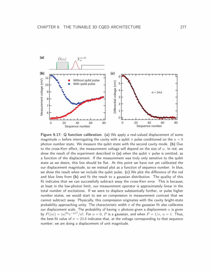
CHAPTER 9. THE TUNABLE 3D CQED ARCHITECTURE 277
6
5
4
3
2
1
0D
iffer
entia
l vol
tage
(mV
)
806040200Sequence number
= 24.6
11
10
9
8
7
6Mea
sure
men
t vol
tage
(mV
)
806040200Sequence number
Without qubit pulse With qubit pulse
(a)
(b) (c)
D(α) Xn=0π
Figure 9.17: Q function calibration. (a) We apply a real-valued displacement of somemagnitude α before interrogating the cavity with a qubit π pulse conditioned on the n = 0photon number state. We measure the qubit state with the second cavity mode. (b) Dueto the cross-Kerr effect, the measurement voltage will depend on the size of α. In red, weshow the result of the experiment described in (a) when the qubit π pulse is omitted, asa function of the displacement. If the measurement was truly only sensitive to the qubitstate as we desire, this line should be flat. At this point we have not yet calibrated theour displacement magnitude, so we instead plot as a function of sequence number. In blue,we show the result when we include the qubit pulse. (c) We plot the difference of the redand blue lines from (b) and fit the result to a gaussian distribution. The quality of thisfit indicates that we can successfully subtract away the cross-Kerr error. This is because,at least in the low-photon limit, our measurement operator is approximately linear in thetotal number of excitations. If we were to displace substantially further, or pulse highernumber states, we would start to see an compression in measurement contrast that wecannot subtract away. Physically, this compression originates with the cavity bright-stateprobability approaching unity. The characteristic width σ of the gaussian fit also calibratesour displacement scale. The probability of having n photons given a displacement α is givenby P (|α|) = |α|2ne−|α|2/n!. For n = 0, P is a gaussian, and when P = 1/e, α = 1. Thus,the best-fit value of σ = 24.6 indicates that, at the voltage corresponding to that sequencenumber, we are doing a displacement of unit magnitude.
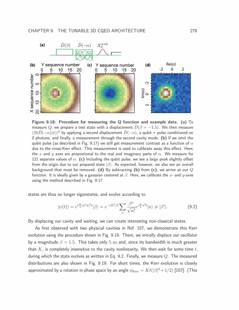
CHAPTER 9. THE TUNABLE 3D CQED ARCHITECTURE 278
Figure 9.18: Procedure for measuring the Q function and example data. (a) Tomeasure Q, we prepare a test state with a displacement D(β = −1.5). We then measure|〈0|D(−α)|ψ〉|2 by applying a second displacement D(−α), a qubit π pulse conditioned on0 photons, and finally, a measurement through the second cavity mode. (b) If we omit thequbit pulse (as described in Fig. 9.17) we still get measurement contrast as a function of αdue to the cross-Kerr effect. This measurement is used to calibrate away this effect. Here,the x and y axes are proportional to the real and imaginary parts of α. We measure for121 separate values of α. (c) Including the qubit pulse, we see a large peak slightly offsetfrom the origin due to our prepared state |β〉. As expected, however, we also see an overallbackground that must be removed. (d) By subtracting (b) from (c), we arrive at our Qfunction. It is ideally given by a gaussian centered at β. Here, we calibrate the x- and y-axesusing the method described in Fig. 9.17.
states are thus no longer eigenstates, and evolve according to
|ψ(t)〉 = eiK2(a†a)2t|β〉 = e−|β|2/2∑
n
βn
√n!ei
K2n2t|n〉 �= |β′〉. (9.2)
By displacing our cavity and waiting, we can create interesting non-classical states.As first observed with two physical cavities in Ref. 107, we demonstrate this Kerr
evolution using the procedure shown in Fig. 9.19. There, we initially displace our oscillatorby a magnitude β = 1.5. This takes only 5 ns and, since its bandwidth is much greaterthan K, is completely insensitive to the cavity nonlinearity. We then wait for some time t,during which the state evolves as written in Eq. 9.2. Finally, we measure Q. The measureddistributions are also shown in Fig. 9.19. For short times, the Kerr evolution is closelyapproximated by a rotation in phase space by an angle φKerr = Kt(|β|2+1/2) [107]. (This
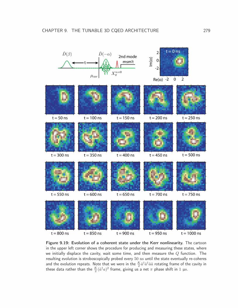
CHAPTER 9. THE TUNABLE 3D CQED ARCHITECTURE 279
Figure 9.19: Evolution of a coherent state under the Kerr nonlinearity. The cartoonin the upper left corner shows the procedure for producing and measuring these states, wherewe initially displace the cavity, wait some time, and then measure the Q function. Theresulting evolution is stroboscopically probed every 50 ns until the state eventually re-coheresand the evolution repeats. Note that we were in the K
2 a†a†aa rotating frame of the cavity in
these data rather than the K2 (a
†a)2 frame, giving us a net π phase shift in 1 μs.
CHAPTER 9. THE TUNABLE 3D CQED ARCHITECTURE 280
fact was used to measure even smaller values of K by compensating with larger α, but inpractice it is considerably more cumbersome than the procedure described in section 9.2.5.)For longer times, the state spreads angularly because amplitude components further fromthe origin rotate with a larger velocity due to the n2 dependence of the Kerr effect. Aftera time Trev = 2π
K≈ 1 μs, the state revives to a coherent state, but with a −1 phase since
eiK2n2t = (−1)n for t = Trev [265]. There a small tail is visible due to inhomogenous cavity
dephasing inherited from the qubit.The state appears to be much more complicated between this early spreading out and
the eventual revival. For example, we see at t ≈ 450 ns that our state is two distinct blobs.This is a superposition of |β〉 and |−β〉, and is known as a “Schrödinger cat” state. Thename refers to the fact that it is a superposition of “alive” and “dead” macroscopic quantumstates. Although it is difficult to resolve with this relatively small initial displacement β,the Kerr evolution in general produces a superposition of an arbitrarily large number ofevenly-spaced coherent states. For integer fractions q of Trev, we can write the quantumstate as [107, 266] ∣∣∣∣ψ(Trev
q
)⟩=
1
2q
2q−1∑p=0
2q−1∑k=0
eik(k−p)πq
∣∣∣βeipπq
⟩. (9.3)
This is a “multi-component Schrödinger cat” state and is made up of q coherent states.Note that the cat shown at t = 450 ns should be exactly symmetric, but is not. Weattribute this to the cavity having substantial higher-order nonlinearity due to its extremelystrong coupling with the qubit. If we move the qubit slightly away to slow down the Kerrevolution, the cats appear to be more symmetric (data not shown).
9.3.3 Freezing Schrödinger cats
The Kerr evolution therefore gives us the ability to create interesting non-classical statesof light. However, the evolution shown in Fig. 9.19 loops around forever, or at leastuntil the state decays to 0 photons and becomes an eigenstate of the Kerr Hamiltonian.If we stored some quantum information in this cavity, it would only be accessible everyTrev. Fortunately, we can eliminate this restriction by using our fast flux control. As weshowed in Fig. 9.14, we can turn K down to essentially zero by detuning the qubit. Wecan therefore start with the qubit near fmax to create some quantum state with the Kerrevolution or direct cavity pulses and then move it away to freeze the evolution of that
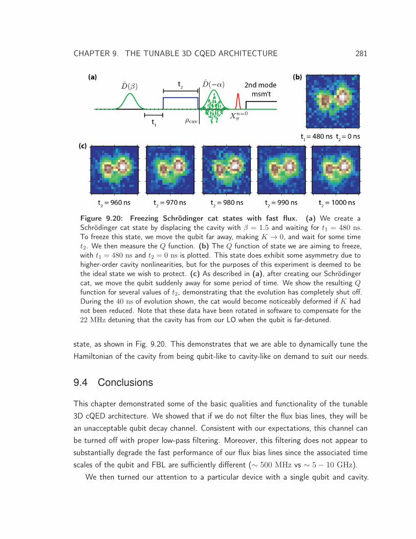
CHAPTER 9. THE TUNABLE 3D CQED ARCHITECTURE 281
Figure 9.20: Freezing Schrödinger cat states with fast flux. (a) We create aSchrödinger cat state by displacing the cavity with β = 1.5 and waiting for t1 = 480 ns.To freeze this state, we move the qubit far away, making K → 0, and wait for some timet2. We then measure the Q function. (b) The Q function of state we are aiming to freeze,with t1 = 480 ns and t2 = 0 ns is plotted. This state does exhibit some asymmetry due tohigher-order cavity nonlinearities, but for the purposes of this experiment is deemed to bethe ideal state we wish to protect. (c) As described in (a), after creating our Schrödingercat, we move the qubit suddenly away for some period of time. We show the resulting Qfunction for several values of t2, demonstrating that the evolution has completely shut off.During the 40 ns of evolution shown, the cat would become noticeably deformed if K hadnot been reduced. Note that these data have been rotated in software to compensate for the22 MHz detuning that the cavity has from our LO when the qubit is far-detuned.
state, as shown in Fig. 9.20. This demonstrates that we are able to dynamically tune theHamiltonian of the cavity from being qubit-like to cavity-like on demand to suit our needs.
9.4 Conclusions
This chapter demonstrated some of the basic qualities and functionality of the tunable3D cQED architecture. We showed that if we do not filter the flux bias lines, they will bean unacceptable qubit decay channel. Consistent with our expectations, this channel canbe turned off with proper low-pass filtering. Moreover, this filtering does not appear tosubstantially degrade the fast performance of our flux bias lines since the associated timescales of the qubit and FBL are sufficiently different (∼ 500 MHz vs ∼ 5 − 10 GHz).
We then turned our attention to a particular device with a single qubit and cavity.
CHAPTER 9. THE TUNABLE 3D CQED ARCHITECTURE 282
The qubit maximum frequency was very close to resonance, making it possible to directlyRabi oscillate the cavity and create photon number Fock states. Combined with fast fluxcontrol, this enabled us to perform a variety of characterization experiments. We showedhow we can directly measure the lifetime and coherence of the cavity as a function of qubitfrequency, demonstrating that the cavity inherits substantial dephasing from the qubit. Wewere able to directly measure and instantaneously control the cavity Kerr anharmonicityand the dispersive χ shift. These experiments primarily serve as an explanation of thekinds of techniques and tools that are available with fast flux control, though also providea rich dataset for validating theoretical predictions.
Finally, motivated by the promising qualities of the 3D cavities, we introduced some basictools for manipulating and measuring continuous-variable quantum states. In particular,we showed how to measure the Husimi Q quasi-probability distribution using the tools wehave already established. Using the Q distribution, we measured the Kerr evolution of acoherent state stored in our nonlinear cavity. At a particular time, this evolution maps usto a superposition of two coherent states known as a Schrödinger cat state. Using fastflux, we froze the evolution of this state, demonstrating our ability to dynamically changethe cavity between an anharmonic qubit-like system to a linear memory. In the next andfinal chapter of this thesis, we will further explore this idea to motivate future applicationsof the tunable 3D architecture.
CHAPTER 10
Conclusions and Future Work
During the last several years, superconducting circuits have made dramatic progressin both complexity and coherence time. We have highlighted these trends in this
thesis, culminating respectively with the demonstration of the most basic form of quantumerror correction and the development of the tunable 3D cQED architecture. Whilesome breakthroughs such as the high-power readout mechanism were unexpected, otherprogressive trends were more purposeful. Increasing from two entangled qubits to threewas primarily a matter of improved engineering. Similarly, the three-qubit Toffoli gaterequired for error correction was a logical progression from the two-qubit gates pioneered inearlier work. (The improved coherence of 3D cQED lies somewhere in between these twoextremes, as it was guided by principle but still exploratory.) The fact that these devicesare so well understood that they can be expanded and built upon speaks to the advantagesof a solid-state quantum architecture. Better understanding of physics and developmentof techniques can be leveraged to do progressively more sophisticated experiments. Indeed,many high-profile results have become standard techniques for later experiments.
The experimental path thus far has largely followed that of earlier systems like NMR andtrapped ions [267]. We have now accomplished many of the “proof-of-principle” experimentswhere any level of functionality can evidence success, but future quantum information goalsare qualitatively different. New landmarks will require combining increased device complexity
283
CHAPTER 10. CONCLUSIONS AND FUTURE WORK 284
with higher gate and measurement fidelity. One such goal is to demonstrate a logical qubitwith a lowered effective error rate using quantum error correction. This has never beenaccomplished in any system despite the fact that the whole future of quantum computing ispredicated on its success. While there are a variety of proposals [17, 18, 68, 80, 90, 91, 93],a great deal of theoretical interest and, more recently, experimental ambition [54, 268] hasconcerned the “surface code” [80, 90, 91]. This code has advantages of a high threshold(∼ 1%) and simple hardware requirements. However, the signature of an operationalsurface code – an improved logical error rate – only emerges from the collective behaviorof a large number of qubits. Even assuming gate fidelities continue to increase, it is hardto imagine fewer than one hundred qubits being used in an initial demonstration. Andif merely controlling one hundred qubits is not challenging enough, each of them mustbe endowed with record-breaking gate fidelity and high fidelity in-situ readout and reset.Progress is being made on each requirement [54, 60, 61, 143, 161, 169, 172, 207], butcombining all those advances with a large number of coupled qubits is a much biggerchallenge.
Fortunately, there are more direct paths to interesting scientific results. One example isthe recent proposal of Leghtas, et al. to error correct a quantum state stored in the Hilbertspace of a harmonic oscillator [92]. It is not yet known to be fault tolerant and does notyet enjoy the considerable theoretical support of the surface code, but it is much simpler toimplement. None of the experimental requirements seem beyond the reach of an academicgroup in the coming years, and several would constitute a high-profile result in their ownright. Moreover, for plausible experimental parameters, this “cat code” could realize animproved effective cavity coherence time. There is also ongoing theoretical developmentof the idea, which might lead to a fault-tolerant implementation that eliminates the needfor a more technical approach like the surface code.
In this chapter, we propose a series of experiments to expand on the work presented inthis thesis. We will start with a list of technical improvements that could be incorporatedinto the tunable 3D cQED architecture (section 10.1). Some of these are straightforwardextensions of what has already been demonstrated, while others are more exploratoryand aspirational. We will then summarize a few exciting qubit experiments that couldbe achieved with an improved 3D cQED or a similar architecture (section 10.2) beforeconcluding with a general outlook on superconducting quantum computing.
CHAPTER 10. CONCLUSIONS AND FUTURE WORK 285
10.1 Tunable 3D cQED development
A considerable amount of development of the 3D cQED architecture has already occurred,but there is room for more. One promising example is to replace the flux bias lines withmicrowave resonators for individual qubit readout. We already have high-bandwidth RFconnectors on the PC board for flux control, so this would be a simple matter of a newlithographic design of the FBL. It may also be possible to design a circuit that could beused for both flux bias and microwave cavity coupling because the relevant frequencies areso different. Additionally, because the FBL wafer is so large, it would be easy to integratecomplications like a Purcell filter to the output of the resonator. This would enable efficientqubit reset, as we saw in section 6.2.4. When combined with a quantum-limited amplifier[61, 190–193, 195, 269, 270], a Purcell-filtered resonator would also enable high-fidelityand QND dispersive measurements.
A resonant structure like the Purcell filter may also represent a better way to design3D FBL lines. In addition to being easier to fabricate, it would eliminate the need for thedielectric capacitors that might currently be limiting coherence. We could also investigatethe dependence of qubit lifetime on physical dimensions. We have already seen that movingfrom a 50 μm to a 300 μm antenna pitch improves qubit lifetime considerably; there maybe other simple and effective changes available to us that have not been tried. Similarly,we could measure flux noise density as a function of the size of our SQUID loop to see ifprogress could be made on that front. Recently, there has also been promising work onusing surface treatments to cut down flux noise [271]. We have not ruled out the possibilitythat our flux noise is the result of a technical problem with the experimental setup, sotesting a tunable 3D cQED device in another fridge would be informative. Improvedcryogenic filtering might also ameliorate qubit lifetimes, and validating our setup againstothers that are known to be of high quality would be reassuring.
Larger architectural design changes are also worth consideration. There have been someissues with RF coupler cross-talk in multi-cavity designs that could be solved by re-designingthe octobox sample holder. We could retrofit the design to support a waveguide Purcellfilter [202] if we wished to measure through a low-Q 3D resonator. A re-design couldalso render more robust the use of high-purity aluminum cavities. The required etchingof these cavities increases physical gaps, which can cause problems when we are relyingon tight fits to confine microwaves in the normal design. An RF choke [170, 272] mayimprove shorting the two sides of the cavity together. Particularly when sapphire wafers

CHAPTER 10. CONCLUSIONS AND FUTURE WORK 286
are present, the quality of the connection between the two sides could dominate the cavityquality factor. Finally, we could scale the architecture to support more cavities and qubitsas experimental requirements dictate.
10.2 Qubit experiments
Though many of the straightforward quantum information experiments have been done,there are a wealth of future directions for superconducting qubits. As ever, we want toimprove qubit gate and measurement fidelity, inventing more robust or scalable multi-qubit gates, and investing in technical capabilities like FPGAs for real-time measurementprocessing [172, 173, 208].
Thinking about the architecture of a large-scale quantum computer has becomeincreasingly necessary. One issue that must soon be addressed is that superconductingqubits tend to interact with one another, particularly when they mutually coupled to thesame cavity. Implementing the surface on a large-scale quantum computer will requirerestricting the length scale of these interactions. As we discuss below, one approach isto make “modules” that interact only through an explicit measurement. This has theadvantages of eliminating any spurious interactions and of being scalable, though it alsosomewhat increases physical overhead.
We will also provide a few examples of interesting experiments that can be done withcurrent (or soon-to-be current) multi-cavity devices. Having multiple cavities enablesconceptually new experiments like entanglement distillation and syndrome extraction, bothof which are necessary for fault-tolerant error correction.
10.2.1 Modules
One challenge with scaling to larger superconducting cQED systems is that qubits tend tointeract with one another over relatively large length scales. While this opens up a varietyof ways to generate multi-qubit gates [55, 121, 169, 176, 201, 209, 232, 252], it presentsa challenge for single-qubit rotations [54, 169, 182, 208]. As we saw in section 5.2.3,even two qubits in a single cavity can have dramatic implications for maintaining controlover each qubit individually. To a certain extent, composite pulses and understandingthe details of these interactions can mitigate the control problem, but these long-rangeinteractions also tend to propagate errors to other qubits, creating a nightmare for fault
CHAPTER 10. CONCLUSIONS AND FUTURE WORK 287
tolerance (section 2.3.6). Though it would be possible to fabricate a device with a largenumber of qubits, accurately controlling and error-correcting such a system will requirelimiting the range of these interactions.
One approach to controlling those interactions is to physically break the connectionbetween qubits. Suppose we have some relatively small system of a few qubits and severalcavities. If we understood the details of all of the (finite number of) interactions wellenough, we might control each qubit with extremely high fidelity. We could then network apair of these smaller devices together via a dispersive measurement that bounces off bothdevices prior to being detected [218–220]. These modules may be separated by relativelylarge distances (the length of an SMA cable) and would only interact via the intentionalmeasurements. Entanglement between devices is heralded by this measurement, whichmight be repeated or “distilled” if the interactions between modules prove faulty. Thisapproach is advantageous in that it is the only currently known way to robustly scalesuperconducting qubits, and because it has a straightforward experimental path.
What are the initial steps along that path? First, we need to develop better toolsfor predicting the higher-order terms of a Hamiltonian and the Purcell effect. Black-boxquantization [138] has been shown to work well for one qubit and cavity, but more workis necessary to take into account multiple qubits and cavities, especially when EC is notsmall. Validating these theoretical calculations will require a detailed measurement of allthe couplings in a system, and performing those measurements as a function of qubitfrequency via flux bias line or external-coil tuning would be even better.
Developing the technology to measure multiple physical cavities is also important. Oneapproach is making two systems with the same cavity frequency and χ-shift, and connectthem with circulators and cables that are as low-loss as possible. As of the writing of thisthesis, the first results of this experiment were just announced out of Irfan Siddiqui’s labin Berkeley [273]. Another approach is to connect the cavities to the signal and idler portsof a JPC amplifier [61, 270], which would eliminate the requirement for circulators priorto amplification and for the cavities to be at the same frequency [274].
10.2.2 Multi-cavity experiments
There are also a variety of interesting qubit experiments which take advantage of havingmore than one cavity which are currently possible or will be soon. Most multi-qubitexperiments conducted so far have involved several qubits in the same cavity. Even if we
CHAPTER 10. CONCLUSIONS AND FUTURE WORK 288
do not use the module approach, we clearly need to limit the number of qubits that directlycouple to one another in order to scale larger. Fortunately, we already have a prototypicalsystem with which to study this idea: the two-cavity 3D cQED device (section 4.2.2).There, we have a single qubit coupled to both cavities, and can have several coupled toeach individual cavity. This enables two conceptual classes of experiments: entanglementdistillation and syndrome extraction.
Entanglement distillation
Entanglement distillation is a process by which we take many imperfect Bell pairs sharedbetween two locations and convert them into a smaller number of higher-fidelity pairs[68, 163–165]. Suppose that we can generate entanglement between distant qubits, perhapsby shuttling excitations through a qubit that is coupled to both. Entanglement generatedin this way will likely be lower fidelity than operations limited to inside a given cavity.For example, the coherence time of the shuttle qubit will be inferior to the single-cavityqubits if the shuttler is flux sensitive and the others fixed-tuned. By repeatedly measuringquantities about the two pairs, we can increase the fidelity of the pairs (conditioned onthe “favorable” outcomes of random measurements).
The most basic type of entanglement distillation would require five qubits in cQED:one ancilla qubit and one communication qubit per cavity, and one shuttle qubit coupledto both cavities∗. We also require the ability to measure both ancilla qubits individually.That protocol [275, 276] begins by entangling two communication qubits by some processthat is assumed to be relatively low fidelity. The communication qubits are then entangledwith the ancilla qubits and subsequently measured along some basis. If the results ofboth measurements are favorable and the fidelity of both the ancilla-communicationentanglement and the measurements are high, then the resulting entanglement fidelitybetween the communication qubits is increased. If the measurement outcome is unfavorable,however, the entanglement may either have been destroyed or reduced in fidelity, dependingon the protocol. Fortunately, with at least some schemes [275], the probability of findingsubsequent favorable measurements increases with each successful repetition.
This general scheme – in which ancillas are measured and a “good” result increasesfidelity – is also used in other QI protocols. For example, there is no known way to
∗ The fifth qubit is not required, but some mechanism to controllably entangle the two distant sets isnecessary.
CHAPTER 10. CONCLUSIONS AND FUTURE WORK 289
fault-tolerantly implement non-Clifford gates like T = e−iπZ/8 in certain error correctionprotocols like the surface code [68]. This gate is needed for universality, so anotherapproach is crucial. One method is known as “magic state distillation” [277, 278]. There, kimperfect copies of the state |A〉 = T |+〉 ∼ |0〉+ eiπ/4|1〉 are generated. These states arethen entangled with one another and various Clifford projections are measured. If all themeasurements are found to have the value +1, we will have k higher-fidelity copies of |A〉.This protocol can be repeated to enhance the fidelity of |A〉 to the effective logical errorrate of our computer, and then teleported into the circuit to implement T as necessary.
Syndrome extraction
All error correction protocols rely on extracting error syndromes from encoded logicalqubits. As we saw in section 2.3.4, this information can either be fed into a quantumgate to implement a correction or it can be measured, classically processed, and fed back.It turns out that measuring the error syndromes is a much more effective method, sinceclassical logic operations can be essentially perfect. This dramatically lowers the overheadassociated with fault-tolerant error correction. However, extracting these syndromes is achallenge itself. In cQED, measurement of transmission through a cavity projects everyqubit coupled to that cavity. If we intend to measure only one ancilla qubit that containssome error syndrome, we would have to use an individual cavity coupled solely to thatqubit. This is one of the motivations for replacing or supplementing FBLs with cavities, aswe have previously discussed.
A method that avoids the need for individual cavities for syndrome extraction wasrecently proposed [168]. There, we have a manifold of N qubits coupled to the samecavity. By using the dispersive χ-shift and a cavity displacement, we can map the valueof any Pauli correlation to the quantum state of the cavity. The cavity will either bein the state |+α〉 or |−α〉 depending on whether the value of some observable is +1
or −1. This observable can be chosen arbitrarily by performing rotations on the qubitsand by echoing away the χ-shifts of qubits that should not be measured. The state ofthe cavity is then read out with some ancilla that is coupled to both the primary cavityand a secondary cavity. It is convenient for that qubit to be flux-tunable to control itsdispersive coupling to the storage cavity. Since this qubit will be entangled with the valueof the syndrome, measuring it will project the system as desired in QEC. Moreover, withrecent developments of fast FPGA logic [172, 173] and low-noise amplifiers [60, 61], a
CHAPTER 10. CONCLUSIONS AND FUTURE WORK 290
high-fidelity QND measurement could be repeated several times. Based on the outcomesof several repetitions, one could, for example, prepare some known entangled Bell or GHZstate.
10.3 Outlook on a superconducting quantum computer
Despite the inevitable challenges, there are many reasons to be optimistic about the futureof superconducting qubits. Only fourteen years have passed since the first Rabi oscillationsof a Cooper pair box were demonstrated at NEC [134]. Since then, there have been vastimprovements to all aspects of the technology. One of the most important advances hasbeen in coherence time. Superconducting qubit coherence has improved nearly five ordersof magnitude since 1999, from 2 ns to ∼ 200 μs. This is of key importance becausecoherence had long been the most pressing open question in evaluating the prospectsof a superconducting quantum computer. In contrast to systems like quantum dots,the source of this decoherence is not known, and it was feared to be an intrinsic limitof Josephson junctions. Recent results [63, 64, 169, 173, 279] have shown that thesejunctions are perfect, at least to the limits of our ability to measure them. Dielectric lossesand thermalization were likely the sources of the previous ∼ μs ceiling. Moreover, sincethe original demonstration of 3D cQED, transmon coherence has improved by anotherfactor of four [162] and further advances are hopefully on their way. Two-dimensionalcQED has also enjoyed impressive advances in coherence, with recent devices exhibiting20−60 μs T2 times [63, 268]. It is fair to say that coherence time no longer represents theprimary obstacle to a superconducting quantum computer, though there always remainsroom for improvement.
In contrast to the problem of coherence time for which the origin and solution wereunknown, many of the current and upcoming challenges are better defined. We need tocontinue making advances with gate fidelity and figure out how to scale to larger systemswithout sacrificing that progress. There is a significant difference between demonstratingfault-tolerant fidelities in a system with only two qubits and demonstrating the same in asystem with a hundred. This creates a conflict: how can we learn to improve gate fidelityin a system that does not yet exist? Or rather, how can we design an architecture thattakes full advantage of the tricks and improvements we have gleaned from smaller devices?One short-term tactic would be to separate the problems of fidelity and scaling into tworesearch avenues. We can continue studying how to improve the coherence and fidelity of

CHAPTER 10. CONCLUSIONS AND FUTURE WORK 291
relatively small systems while simultaneously thinking about ways to scale to large ones[250, 268]. Investigating how to mitigate spurious long-distance communication is animportant concern, but has ample room for innovation and creativity.
Fortunately, the challenge of scaling plays directly into the strengths of superconductingqubits. Unlike previous quantum architectures, cQED devices are solid-state systemsfabricated in a clean room and controlled with electronic signals. (This statement disregardsthe fact that 3D cavities are made in a machine shop, since there is no reason to believethat is a requirement.) These properties of superconducting qubits are reminiscent of thesilicon transistor, the most replicated human-made object in history. It seems likely thatmethods of inhibiting qubit cross-talk, constructing high-fidelity gates, and implementingroom-temperature control will all be soon in coming. These will clear the way to scalingto very large superconducting devices, and potentially, a true quantum computer.
��


Bibliography
1. A. Einstein, B. Podolsky, and N. Rosen, “Can quantum-mechanical description ofphysical reality be considered complete?,” Phys. Rev. 47, 777–780 (1935). Cited onpages 2 & 213.
2. F. Wilczek, “Quantum field theory,” Rev. Mod. Phys. 71, S85–S95 (1999). Cited onpage 2.
3. G. Gabrielse, D. Hanneke, T. Kinoshita, M. Nio, and B. Odom, “New Determinationof the Fine Structure Constant from the Electron g Value and QED,” Phys. Rev.Lett. 97, 030802 (2006). Cited on page 2.
4. G. Gabrielse, D. Hanneke, T. Kinoshita, M. Nio, and B. Odom, “Erratum: NewDetermination of the Fine Structure Constant from the Electron g Value and QED[Phys. Rev. Lett. 97, 030802 (2006)],” Phys. Rev. Lett. 99, 039902 (2007). Citedon page 2.
5. J. S. Bell, “On the Einstein Podolsky Rosen Paradox,” Physics 1, 195–200 (1964).Cited on page 2.
6. A. Aspect, P. Grangier, and G. Roger, “Experimental Tests of Realistic LocalTheories via Bell’s Theorem,” Phys. Rev. Lett. 47, 460–463 (1981). Cited on page 2.
7. W. K. Wootters and W. H. Zurek, “A single quantum cannot be cloned,” Nature299, 802–803 (1982). Cited on pages 3 & 32.
8. S. Wiesner, “Conjugate coding,” Sigact News 15, 78 (1983). Cited on page 3.
9. C. H. Bennett and G. Brassard, “Quantum cryptography: Public key distribution andcoin tossing,” Proceedings of IEEE International Conference on Computers, Systemsand Signal Processing 175–179 (1984). Cited on page 3.
293
BIBLIOGRAPHY 294
10. D. Kaiser, How the Hippies Saved Physics. W. W. Norton & Company, 2012. Citedon page 3.
11. R. P. Feynman, “Simulating physics with computers,” International Journal ofTheoretical Physics 21, 467–488 (1982). Cited on page 3.
12. D. Deutsch, “Quantum Theory, the Church-Turing Principle and the UniversalQuantum Computer,” Proceedings of the Royal Society of London. A. Mathematicaland Physical Sciences 400, 97–117 (1985). Cited on page 3.
13. D. Deutsch and R. Jozsa, “Rapid solution of problems by quantum computation,”Proc. R. Soc. Lond. A 439, 553–558 (1992). Cited on pages 3 & 25.
14. P. W. Shor, “Polynomial-time algorithms for prime factorization and discretelogarithms on a quantum computer,” SIAM J. Sci. Statist. Comput. 26, 1484(1995). Cited on pages 3, 25 & 220.
15. R. Rivest, A. Shamir, and L. Adleman, “A method for obtaining digital signaturesand public-key cryptosystems,” Communications of the ACM 21, 120–126 (1978).Cited on page 3.
16. S. J. Devitt, A. G. Fowler, and L. C. L. Hollenberg, “Robustness of Shor’s algorithm,”Quant. Inf. Comp. 6, 616–629 (2006). Cited on page 4.
17. P. W. Shor, “Scheme for reducing decoherence in quantum computer memory,” Phys.Rev. A 52, R2493–R2496 (1995). Cited on pages 4, 41, 251 & 284.
18. A. Steane, “Multiple-particle interference and quantum error correction,”Proceedings of the Royal Society of London. Series A: Mathematical, Physical andEngineering Sciences 452, 2551–2577 (1996). Cited on pages 4, 42, 43 & 284.
19. R. Laflamme, C. Miquel, J. P. Paz, and W. H. Zurek, “Perfect quantum errorcorrecting code,” Phys. Rev. Lett. 77, 198–201 (1996). Cited on pages 4 & 42.
20. P. W. Shor, “Fault-tolerant quantum computation,” ArXiv e-prints (1996),arXiv:quant-ph/9605011. Cited on pages 4, 28 & 43.
21. I. L. Chuang, N. Gershenfeld, and M. Kubinec, “Experimental implementation of fastquantum searching,” Phys. Rev. Lett. 80, 3408–3411 (1998). Cited on page 4.
22. I. L. Chuang, L. M. K. Vandersypen, X. Zhou, D. W. Leung, and S. Lloyd,“Experimental realization of a quantum algorithm,” Nature 393, 143–146 (1998).Cited on page 4.
23. J. A. Jones, M. Mosca, and R. H. Hansen, “Implementation of a quantum searchalgorithm on a quantum computer,” Nature 393, 344–346 (1998). Cited on page 4.
BIBLIOGRAPHY 295
24. L. M. K. Vandersypen, M. Steffen, G. Breyta, C. S. Yannoni, M. H. Sherwood, andI. L. Chuang, “Experimental realization of Shor’s quantum factoring algorithm usingnuclear magnetic resonance,” Nature 414, 883–887 (2001). Cited on page 4.
25. W. S. Warren, “The usefulness of NMR quantum computing,” Science 277,1688–1690 (1997). Cited on pages 4 & 47.
26. J. I. Cirac and P. Zoller, “Quantum computations with cold trapped ions,” Phys.Rev. Lett. 74, 4091–4094 (1995). Cited on pages 4 & 47.
27. D. Leibfried, R. Blatt, C. Monroe, and D. Wineland, “Quantum dynamics of singletrapped ions,” Rev. Mod. Phys. 75, 281–324 (2003). Cited on pages 4 & 47.
28. D. Leibfried, B. DeMarco, V. Meyer, D. Lucas, M. Barrett, J. Britton, W. M. Itano,B. Jelenković, C. Langer, T. Rosenband, and D. J. Wineland, “Experimentaldemonstration of a robust, high-fidelity geometric two ion-qubit phase gate,” Nature422, 412–415 (2003). Cited on page 4.
29. K. Singer, U. Poschinger, M. Murphy, P. Ivanov, F. Ziesel, T. Calarco, andF. Schmidt-Kaler, “Colloquium : Trapped ions as quantum bits: Essential numericaltools,” Rev. Mod. Phys. 82, 2609–2632 (2010). Cited on pages 4 & 47.
30. P. Schindler, J. T. Barreiro, T. Monz, V. Nebendahl, D. Nigg, M. Chwalla,M. Hennrich, and R. Blatt, “Experimental repetitive quantum error correction,”Science 332, 1059–1061 (2011). Cited on pages 4, 47, 219 & 248.
31. C. Monroe and J. Kim, “Scaling the ion trap quantum processor,” Science 339,1164–1169 (2013). Cited on pages 4 & 47.
32. A. H. Myerson, D. J. Szwer, S. C. Webster, D. T. C. Allcock, M. J. Curtis, G. Imreh,J. A. Sherman, D. N. Stacey, A. M. Steane, and D. M. Lucas, “High-fidelity readoutof trapped-ion qubits,” Phys. Rev. Lett. 100, 200502 (2008). Cited on page 4.
33. J. P. Gaebler, A. M. Meier, T. R. Tan, R. Bowler, Y. Lin, D. Hanneke, J. D. Jost,J. P. Home, E. Knill, D. Leibfried, and D. J. Wineland, “Randomized benchmarkingof multiqubit gates,” Phys. Rev. Lett. 108, 260503 (2012). Cited on pages 4 & 132.
34. T. Monz, P. Schindler, J. T. Barreiro, M. Chwalla, D. Nigg, W. A. Coish,M. Harlander, W. Hänsel, M. Hennrich, and R. Blatt, “14-Qubit Entanglement:Creation and Coherence,” Phys. Rev. Lett. 106, 130506 (2011). Cited onpages 4 & 5.
35. D. Kielpinski, C. Monroe, and D. J. Wineland, “Architecture for a large-scaleion-trap quantum computer,” Nature 417, 709–711 (2002). Cited on page 5.
BIBLIOGRAPHY 296
36. D. Stick, W. K. Hensinger, S. Olmschenk, M. J. Madsen, K. Schwab, andC. Monroe, “Ion trap in a semiconductor chip,” Nature Physics 2, 36–39 (2006).Cited on page 5.
37. S. X. Wang, Y. Ge, J. Labaziewicz, E. Dauler, K. Berggren, and I. L. Chuang,“Superconducting microfabricated ion traps,” Appl. Phys. Lett. 97, 244102 (2010).Cited on page 5.
38. E. Schrodinger, “Are there quantum jumps? Part II,” Brit. J. Phil. Sci. 3, 233–242(1952). Cited on page 5.
39. H.-J. Briegel, T. Calarco, D. Jaksch, J. I. Cirac, and P. Zoller, “Quantum computingwith neutral atoms,” Journal of Modern Optics 47, 415–451 (2000). Cited onpage 5.
40. D. Loss and D. P. DiVincenzo, “Quantum computation with quantum dots,” Phys.Rev. A 57, 120–126 (1998). Cited on pages 5 & 47.
41. R. Hanson, L. P. Kouwenhoven, J. R. Petta, S. Tarucha, and L. M. K. Vandersypen,“Spins in few-electron quantum dots,” Rev. Mod. Phys. 79, 1217–1265 (2007).Cited on pages 5 & 47.
42. B. M. Maune, M. G. Borselli, B. Huang, T. D. Ladd, P. W. Deelman, K. S. Holabird,A. A. Kiselev, I. Alvarado-Rodriguez, R. S. Ross, A. E. Schmitz, M. Sokolich, C. A.Watson, M. F. Gyure, and A. T. Hunter, “Coherent singlet-triplet oscillations in asilicon-based double quantum dot,” Nature 481, 344–347 (2012). Cited onpages 5 & 47.
43. M. D. Shulman, O. E. Dial, S. P. Harvey, H. Bluhm, V. Umansky, and A. Yacoby,“Demonstration of Entanglement of Electrostatically Coupled Singlet-Triplet Qubits,”Science 336, 202– (2012). Cited on pages 5 & 47.
44. D. D. Awschalom, L. C. Bassett, A. S. Dzurak, E. L. Hu, and J. R. Petta, “Quantumspintronics: Engineering and manipulating atom-like spins in semiconductors,”Science 339, 1174–1179 (2013). Cited on pages 5 & 47.
45. D. I. Schuster, A. Fragner, M. I. Dykman, S. A. Lyon, and R. J. Schoelkopf,“Proposal for manipulating and detecting spin and orbital states of trapped electronson helium using cavity quantum electrodynamics,” Phys. Rev. Lett. 105, 040503(2010). Cited on page 5.
46. F. Jelezko and J. Wrachtrup, “Single defect centres in diamond: A review,” physicastatus solidi (a) 203, 3207–3225 (2006). Cited on pages 5 & 47.
BIBLIOGRAPHY 297
47. M. V. G. Dutt, L. Childress, L. Jiang, E. Togan, J. Maze, F. Jelezko, A. S. Zibrov,P. R. Hemmer, and M. D. Lukin, “Quantum register based on individual electronicand nuclear spin qubits in diamond,” Science 316, 1312–1316 (2007). Cited onpages 5 & 47.
48. P. C. Maurer, G. Kucsko, C. Latta, L. Jiang, N. Y. Yao, S. D. Bennett, F. Pastawski,D. Hunger, N. Chisholm, M. Markham, D. J. Twitchen, J. I. Cirac, and M. D. Lukin,“Room-temperature quantum bit memory exceeding one second,” Science 336,1283–1286 (2012). Cited on pages 5 & 47.
49. M. H. Devoret and R. J. Schoelkopf, “Superconducting circuits for quantuminformation: An outlook,” Science 339, 1169–1174 (2013). Cited on pages 5 & 47.
50. V. Bouchiat, D. Vion, P. Joyez, D. Esteve, and M. H. Devoret, “Quantum coherencewith a single Cooper pair,” Physica Scripta 1996, 165 (1998). Cited onpages 5 & 50.
51. Y. Makhlin, G. Schön, and A. Shnirman, “Quantum-state engineering withJosephson-junction devices,” Rev. Mod. Phys. 73, 357–400 (2001). Cited on page 5.
52. D. Vion, A. Aassime, A. Cottet, P. Joyez, H. Pothier, C. Urbina, D. Esteve, andM. H. Devoret, “Manipulating the Quantum State of an Electrical Circuit,” Science296, 886–889 (2002). Cited on pages 5, 48 & 50.
53. J. M. Chow, J. M. Gambetta, L. Tornberg, J. Koch, L. S. Bishop, A. A. Houck,B. R. Johnson, L. Frunzio, S. M. Girvin, and R. J. Schoelkopf, “Randomizedbenchmarking and process tomography for gate errors in a solid-state qubit,” Phys.Rev. Lett. 102, 090502 (2009). Cited on pages 5, 58, 132 & 213.
54. J. M. Chow, J. M. Gambetta, A. D. Córcoles, S. T. Merkel, J. A. Smolin, C. Rigetti,S. Poletto, G. A. Keefe, M. B. Rothwell, J. R. Rozen, M. B. Ketchen, andM. Steffen, “Universal quantum gate set approaching fault-tolerant thresholds withsuperconducting qubits,” Phys. Rev. Lett. 109, 060501 (2012). Cited on pages 5,30, 31, 212, 284 & 286.
55. L. DiCarlo, M. D. Reed, L. Sun, B. R. Johnson, J. M. Chow, J. M. Gambetta,L. Frunzio, S. M. Girvin, M. H. Devoret, and R. J. Schoelkopf, “Preparation andmeasurement of three-qubit entanglement in a superconducting circuit,” Nature467, 574–578 (2010). Cited on pages 5, 48, 83, 100, 143, 164, 175, 179, 184, 200,203, 208, 212, 215, 216, 240, 244 & 286.
56. M. Ansmann, H. Wang, R. C. Bialczak, M. Hofheinz, E. Lucero, M. Neeley, A. D.O’Connell, D. Sank, M. Weides, J. Wenner, A. N. Cleland, and J. M. Martinis,“Violation of Bell’s inequality in Josephson phase qubits,” Nature 461, 504–506(2009). Cited on page 5.
BIBLIOGRAPHY 298
57. R. C. Bialczak, M. Ansmann, M. Hofheinz, E. Lucero, M. Neeley, A. D. O/’Connell,D. Sank, H. Wang, J. Wenner, M. Steffen, A. N. Cleland, and J. M. Martinis,“Quantum process tomography of a universal entangling gate implemented withjosephson phase qubits,” Nat. Phys. 6, 409–413 (2010). Cited on page 5.
58. A. Wallraff, D. I. Schuster, A. Blais, L. Frunzio, J. Majer, M. H. Devoret, S. M.Girvin, and R. J. Schoelkopf, “Approaching unit visibility for control of asuperconducting qubit with dispersive readout,” Phys. Rev. Lett. 95, 060501 (2005).Cited on pages 5 & 58.
59. M. D. Reed, L. DiCarlo, B. R. Johnson, L. Sun, D. I. Schuster, L. Frunzio, and R. J.Schoelkopf, “High-fidelity readout in circuit quantum electrodynamics using theJaynes-Cummings nonlinearity,” Phys. Rev. Lett. 105, 173601 (2010). Cited onpages 5, 115, 117, 154, 156, 157, 158, 159, 162, 164, 165 & 176.
60. R. Vijay, D. H. Slichter, and I. Siddiqi, “Observation of quantum jumps in asuperconducting artificial atom,” Phys. Rev. Lett. 106, 110502 (2011). Cited onpages 5, 140, 284 & 289.
61. M. Hatridge, S. Shankar, M. Mirrahimi, F. Schackert, K. Geerlings, T. Brecht, K. M.Sliwa, B. Abdo, L. Frunzio, S. M. Girvin, R. J. Schoelkopf, and M. H. Devoret,“Quantum back-action of an individual variable-strength measurement,” Science 339,178–181 (2013). Cited on pages 5, 14, 47, 140, 141, 284, 285, 287 & 289.
62. H. Paik, D. I. Schuster, L. S. Bishop, G. Kirchmair, G. Catelani, A. P. Sears, B. R.Johnson, M. J. Reagor, L. Frunzio, L. I. Glazman, S. M. Girvin, M. H. Devoret, andR. J. Schoelkopf, “Observation of High Coherence in Josephson Junction QubitsMeasured in a Three-Dimensional Circuit QED Architecture,” Phys. Rev. Lett. 107,240501 (2011). Cited on pages 5, 7, 47, 54, 58, 81, 86, 113, 118, 119, 124,147 & 149.
63. J. Chang, M. R. Vissers, A. Corcoles, M. Sandberg, J. Gao, D. W. Abraham, J. M.Chow, J. M. Gambetta, M. B. Rothwell, G. A. Keefe, M. Steffen, and D. P. Pappas,“Improved superconducting qubit coherence using titanium nitride,” ArXiv e-prints(2013), arXiv:1303.4071. Cited on pages 5, 113, 147 & 290.
64. C. Rigetti, J. M. Gambetta, S. Poletto, B. L. T. Plourde, J. M. Chow, A. D.Córcoles, J. A. Smolin, S. T. Merkel, J. R. Rozen, G. A. Keefe, M. B. Rothwell,M. B. Ketchen, and M. Steffen, “Superconducting qubit in a waveguide cavity with acoherence time approaching 0.1 ms,” Phys. Rev. B 86, 100506 (2012). Cited onpages 7, 87, 113 & 290.
65. J. P. Groen, D. Ristè, L. Tornberg, J. Cramer, P. C. de Groot, T. Picot,G. Johansson, and L. DiCarlo, “Partial-measurement back-action and non-classical

BIBLIOGRAPHY 299
weak values in a superconducting circuit,” ArXiv e-prints (2013), arXiv:1302.5147.Cited on page 14.
66. T. Toffoli, “Reversible computing,” in Automata, Languages and Programming,J. Bakker and J. Leeuwen, eds., vol. 85 of Lecture Notes in Computer Science,pp. 632–644. Springer Berlin Heidelberg, 1980. Cited on page 16.
67. L. Jiang, “Quantum Information and Computation.” Class at Yale University, Spring,2013. Cited on page 18.
68. M. A. Nielsen and I. L. Chuang, Quantum computation and quantum information.Cambridge Series on Information and the Natural Sciences. Cambridge UniversityPress, 2000. Cited on pages 20, 22, 27, 32, 43, 206, 247, 248, 284, 288 & 289.
69. W. Dür, G. Vidal, and J. I. Cirac, “Three qubits can be entangled in two inequivalentways,” Phys. Rev. A 62, 062314 (2000). Cited on page 23.
70. D. M. Greenberger, M. A. Horne, and A. Zeilinger, “Going beyond Bell’s theorem,”in Bell’s theorem, quantum theory and conceptions of the universe, M. Kafatos, ed.Kluwer Academic, Dordrecht, 1989. Cited on pages 23, 209 & 244.
71. T. Bastin, S. Krins, P. Mathonet, M. Godefroid, L. Lamata, and E. Solano,“Operational families of entanglement classes for symmetric n-qubit states,” Phys.Rev. Lett. 103, 070503 (2009). Cited on page 23.
72. A. Peres, “Separability criterion for density matrices,” Phys. Rev. Lett. 77,1413–1415 (1996). Cited on page 24.
73. M. Horodecki, P. Horodecki, and R. Horodecki, “Separability of mixed states:necessary and sufficient conditions,” Physics Letters A 223, 1 – 8 (1996). Cited onpage 24.
74. P. W. Shor, “Why haven’t more quantum algorithms been found?,” J. ACM 50,87–90 (2003). Cited on page 25.
75. P. W. Shor, “Progress in quantum algorthms,” Quantum Information Processing 3,5–13 (2004). Cited on page 25.
76. L. K. Grover, “A fast quantum mechanical algorithm for database search,”Proceedings, 28th ACM Symposium on Theory of Computation 212 (1996). Citedon page 25.
77. L. K. Grover, “Quantum mechanics helps in searching for a needle in a haystack,”Phys. Rev. Lett. 79, 325–328 (1997). Cited on page 25.
BIBLIOGRAPHY 300
78. S. Jordan, “NIST Quantum Algorithm Zoo.” http://math.nist.gov/quantum/zoo/.Cited on page 25.
79. D. P. DiVincenzo, “The physical implementation of quantum computation,” Fortschr.Phys 48, 2000 (2000). Cited on pages 26 & 88.
80. A. G. Fowler, M. Mariantoni, J. M. Martinis, and A. N. Cleland, “Surface codes:Towards practical large-scale quantum computation,” Phys. Rev. A 86, 032324(2012). Cited on pages 27, 28, 29, 43 & 284.
81. D. Gottesman, “Beyond the DiVincenzo criteria: Requirements and desiderata forfault-tolerance,” in In Joint IPAM/MSRI Workshop on Quantum Computing. 2002.Cited on page 28.
82. Q. A. Turchette, C. J. Hood, W. Lange, H. Mabuchi, and H. J. Kimble,“Measurement of conditional phase shifts for quantum logic,” Phys. Rev. Lett. 75,4710–4713 (1995). Cited on page 28.
83. A. Imamoglu, D. D. Awschalom, G. Burkard, D. P. DiVincenzo, D. Loss,M. Sherwin, and A. Small, “Quantum Information Processing Using Quantum DotSpins and Cavity QED,” Phys. Rev. Lett. 83, 4204–4207 (1999). Cited on page 28.
84. K. M. Svore, B. M. Terhal, and D. P. DiVincenzo, “Local fault-tolerant quantumcomputation,” Phys. Rev. A 72, 022317 (2005). Cited on page 28.
85. T. Szkopek, P. Boykin, H. Fan, V. Roychowdhury, E. Yablonovitch, G. Simms,M. Gyure, and B. Fong, “Threshold error penalty for fault tolerant computation withnearest neighbour communication,” IEEE Trans. Nano. 5, 42–49 (2006). Cited onpage 28.
86. S. J. Devitt, A. G. Fowler, T. Tilma, W. J. Munro, and K. Nemoto, “ClassicalProcessing Requirements for a Topological Quantum Computing System,” ArXive-prints (2009), arXiv:0906.0415. Cited on page 28.
87. K. R. Brown, A. C. Wilson, Y. Colombe, C. Ospelkaus, A. M. Meier, E. Knill,D. Leibfried, and D. J. Wineland, “Single-qubit-gate error below 10−4 in a trappedion,” Phys. Rev. A 84, 030303 (2011). Cited on pages 30 & 31.
88. D. Gottesman, Stabilizer Codes and Quantum Error Correction. PhD thesis,California Institute of Technology, 1997. arXiv:quant-ph/9705052. Cited on page 36.
89. A. R. Calderbank and P. W. Shor, “Good quantum error-correcting codes exist,”Phys. Rev. A 54, 1098–1105 (1996). Cited on page 43.
BIBLIOGRAPHY 301
90. A. Kitaev, “Quantum error correction with imperfect gates,” in Proceedings of theThird International Conference on Quantum Communication and Measurement,A. S. H. O. Hirota and C. M. Caves, eds. Plenum, 1997. Cited on pages 43 & 284.
91. S. B. Bravyi and A. Kitaev, “Quantum codes on a lattice with boundary,” ArXive-prints (1998), arXiv:quant-ph/9811052. Cited on pages 43 & 284.
92. Z. Leghtas, G. Kirchmair, B. Vlastakis, M. H. Devoret, R. J. Schoelkopf, andM. Mirrahimi, “Deterministic protocol for mapping a qubit to coherent statesuperpositions in a cavity,” Phys. Rev. A 87, 042315 (2013). Cited on pages 43, 65,87, 275 & 284.
93. Z. Leghtas, G. Kirchmair, B. Vlastakis, R. J. Schoelkopf, M. H. Devoret, andM. Mirrahimi, “Hardware-efficient autonomous quantum error correction,” ArXive-prints (2012), arXiv:1207.0679. Cited on pages 43, 87, 274, 275 & 284.
94. J. Preskill, “Fault tolerant quantum computation,” in Introduction to QuantumComputation, H. K. Lo, S. Popescu, and T. P. Spiller, eds. World Scientific, 1998.quant-ph/9712048. Cited on page 43.
95. D. Gottesman, “An introduction to quantum error correction and fault-tolerantquantum computation,” ArXiv e-prints (2009), arXiv:0904.2557. Cited on page 43.
96. T. D. Ladd, F. Jelezko, R. Laflamme, Y. Nakamura, C. Monroe, and J. L. O’Brien,“Quantum computers,” Nature 464, 45–53 (2010). Cited on page 47.
97. L. M. K. Vandersypen and I. L. Chuang, “NMR techniques for quantum control andcomputation,” Rev. Mod. Phys. 76, 1037–1069 (2005). Cited on page 47.
98. C. A. Ryan, M. Laforest, and R. Laflamme, “Randomized benchmarking of single-and multi-qubit control in liquid-state NMR quantum information processing,” NewJournal of Physics 11, 013034 (2009). Cited on page 47.
99. P. Kok, W. J. Munro, K. Nemoto, T. C. Ralph, J. P. Dowling, and G. J. Milburn,“Linear optical quantum computing with photonic qubits,” Rev. Mod. Phys. 79,135–174 (2007). Cited on page 47.
100. S. Barz, E. Kashefi, A. Broadbent, J. F. Fitzsimons, A. Zeilinger, and P. Walther,“Demonstration of blind quantum computing,” Science 335, 303–308 (2012). Citedon page 47.
101. M. I. Dyakonov, “State of the art and prospects for quantum computing,” ArXive-prints (2012), arXiv:1212.3562. Cited on page 47.
BIBLIOGRAPHY 302
102. C. Nayak, S. H. Simon, A. Stern, M. Freedman, and S. Das Sarma, “Non-abeliananyons and topological quantum computation,” Rev. Mod. Phys. 80, 1083–1159(2008). Cited on page 47.
103. M. Z. Hasan and C. L. Kane, “Colloquium : Topological insulators,” Rev. Mod.Phys. 82, 3045–3067 (2010). Cited on page 47.
104. A. Stern and N. H. Lindner, “Topological quantum computation—from basicconcepts to first experiments,” Science 339, 1179–1184 (2013). Cited on page 47.
105. L. Frunzio, A. Wallraff, D. Schuster, J. Majer, and R. Schoelkopf, “Fabrication andcharacterization of superconducting circuit QED devices for quantum computation,”IEEE Trans. On Appl. Superc. 15, 860 (2005). Cited on pages 48 & 84.
106. A. Blais, R.-S. Huang, A. Wallraff, S. M. Girvin, and R. J. Schoelkopf, “Cavityquantum electrodynamics for superconducting electrical circuits: An architecture forquantum computation,” Phys. Rev. A 69, 062320 (2004). Cited on pages 48,58 & 81.
107. G. Kirchmair, B. Vlastakis, Z. Leghtas, S. E. Nigg, H. Paik, E. Ginossar,M. Mirrahimi, L. Frunzio, S. M. Girvin, and R. J. Schoelkopf, “Observation ofquantum state collapse and revival due to the single-photon Kerr effect,” Nature495, 205–209 (2013). Cited on pages 48, 61, 71, 88, 96, 154, 259, 262, 270, 275,276, 278 & 280.
108. M. Hofheinz, H. Wang, M. Ansmann, R. C. Bialczak, E. Lucero, M. Neeley, A. D.O’Connell, D. Sank, J. Wenner, J. M. Martinis, and A. N. Cleland, “Synthesizingarbitrary quantum states in a superconducting resonator,” Nature 459, 546–549(2009). Cited on page 48.
109. B. R. Johnson, M. D. Reed, A. A. Houck, D. I. Schuster, L. S. Bishop, E. Ginossar,J. M. Gambetta, L. DiCarlo, L. Frunzio, S. M. Girvin, and R. J. Schoelkopf,“Quantum non-demolition detection of single microwave photons in a circuit,” Nat.Phys. 6, 663–667 (2010). Cited on pages 48, 61, 65, 71, 88, 143, 149 & 275.
110. D. Bozyigit, C. Lang, L. Steffen, J. M. Fink, C. Eichler, M. Baur, R. Bianchetti, P. J.Leek, S. Filipp, M. P. da Silva, A. Blais, and A. Wallraff, “Antibunching ofmicrowave-frequency photons observed in correlation measurements using lineardetectors,” Nat. Phys. 7, 154–158 (2011). Cited on page 48.
111. C. Lang, C. Eichler, L. Steffen, J. M. Fink, M. J. Woolley, A. Blais, and A. Wallraff,“Probing Correlations, Indistinguishability and Entanglement in MicrowaveTwo-Photon Interference,” ArXiv e-prints (2013), arXiv:1301.4458. Cited onpage 48.
BIBLIOGRAPHY 303
112. D. Schuster, Circuit Quantum Electrodynamics. PhD thesis, Yale University, 2007.http://www.eng.yale.edu/rslab/papers/SchusterThesis.pdf. Cited on pages 48, 56,58, 59, 66, 82, 114 & 141.
113. L. S. Bishop, Circuit Quantum Electrodynamics. PhD thesis, Yale University, 2010.http://www.levbishop.org/thesis/. Cited on pages 48, 54, 58, 59, 63, 65, 67 & 68.
114. J. M. Chow, Quantum Information Processing with Superconducting Qubits. PhDthesis, Yale University, 2010. http://www.eng.yale.edu/rslab/papers/jmcthesis.pdf.Cited on pages 48, 58, 69, 70, 74, 82, 86, 117, 129 & 203.
115. J. Koch, T. M. Yu, J. Gambetta, A. A. Houck, D. I. Schuster, J. Majer, A. Blais,M. H. Devoret, S. M. Girvin, and R. J. Schoelkopf, “Charge-insensitive qubit designderived from the cooper pair box,” Phys. Rev. A 76, 042319 (2007). Cited onpages 48, 50, 51, 52, 56, 58, 62, 64, 84 & 137.
116. J. Gambetta, W. A. Braff, A. Wallraff, S. M. Girvin, and R. J. Schoelkopf,“Protocols for optimal readout of qubits using a continuous quantum nondemolitionmeasurement,” Phys. Rev. A 76, 012325 (2007). Cited on pages 48, 58, 138,140 & 141.
117. J. A. Schreier, A. A. Houck, J. Koch, D. I. Schuster, B. R. Johnson, J. M. Chow,J. M. Gambetta, J. Majer, L. Frunzio, M. H. Devoret, S. M. Girvin, and R. J.Schoelkopf, “Suppressing charge noise decoherence in superconducting chargequbits,” Phys. Rev. B 77, 180502 (2008). Cited on pages 48, 50 & 156.
118. A. Wallraff, D. I. Schuster, A. Blais, L. Frunzio, R. S. Huang, J. Majer, S. Kumar,S. M. Girvin, and R. J. Schoelkopf, “Strong coupling of a single photon to asuperconducting qubit using circuit quantum electrodynamics,” Nature 431,162–167 (2004). Cited on pages 48, 58, 81 & 82.
119. J. Majer, J. M. Chow, J. M. Gambetta, J. Koch, B. R. Johnson, J. A. Schreier,L. Frunzio, D. I. Schuster, A. A. Houck, A. Wallraff, A. Blais, M. H. Devoret, S. M.Girvin, and R. J. Schoelkopf, “Coupling superconducting qubits via a cavity bus,”Nature 449, 443–447 (2007). Cited on pages 48, 58, 71, 82 & 178.
120. E. Jaynes and F. W. Cummings, “Comparison of quantum and semiclassicalradiation theories with application to the beam maser,” Proceedings of the IEEE 51,89–109 (1963). Cited on page 48.
121. L. DiCarlo, J. M. Chow, J. M. Gambetta, L. S. Bishop, B. R. Johnson, D. I. Schuster,J. Majer, A. Blais, L. Frunzio, S. M. Girvin, and R. J. Schoelkopf, “Demonstration oftwo-qubit algorithms with a superconducting quantum processor,” Nature 460,240–244 (2009). Cited on pages 48, 58, 70, 72, 82, 148, 164, 185, 187 & 286.
BIBLIOGRAPHY 304
122. B. D. Josephson, “Possible new effects in superconductive tunnelling,” PhysicsLetters 1, 251 – 253 (1962). Cited on page 49.
123. B. D. Josephson, “The discovery of tunnelling supercurrents,” Rev. Mod. Phys. 46,251–254 (1974). Cited on page 49.
124. S. Gigan, H. R. Bohm, M. Paternostro, F. Blaser, G. Langer, J. B. Hertzberg, K. C.Schwab, D. Bauerle, M. Aspelmeyer, and A. Zeilinger, “Self-cooling of a micromirrorby radiation pressure,” Nature 444, 67–70 (2006). Cited on page 50.
125. J. D. Thompson, B. M. Zwickl, A. M. Jayich, F. Marquardt, S. M. Girvin, andJ. G. E. Harris, “Strong dispersive coupling of a high-finesse cavity to amicromechanical membrane,” Nature 452, 72–75 (2008). Cited on page 50.
126. A. D. O’Connell, M. Hofheinz, M. Ansmann, R. C. Bialczak, M. Lenander,E. Lucero, M. Neeley, D. Sank, H. Wang, M. Weides, J. Wenner, J. M. Martinis,and A. N. Cleland, “Quantum ground state and single-phonon control of amechanical resonator,” Nature 464, 697–703 (2010). Cited on page 50.
127. J. D. Teufel, T. Donner, D. Li, J. W. Harlow, M. S. Allman, K. Cicak, A. J. Sirois,J. D. Whittaker, K. W. Lehnert, and R. W. Simmonds, “Sideband cooling ofmicromechanical motion to the quantum ground state,” Nature 475, 359–363(2011). Cited on page 50.
128. T. P. Purdy, R. W. Peterson, and C. A. Regal, “Observation of radiation pressureshot noise on a macroscopic object,” Science 339, 801–804 (2013). Cited onpage 50.
129. J. E. Mooij, T. P. Orlando, L. Levitov, L. Tian, C. H. van der Wal, and S. Lloyd,“Josephson persistent-current qubit,” Science 285, 1036–1039 (1999). Cited onpage 50.
130. J. R. Friedman, V. Patel, W. Chen, S. K. Tolpygo, and J. E. Lukens, “Quantumsuperposition of distinct macroscopic states,” Nature 406, 43–46 (2000). Cited onpage 50.
131. I. Chiorescu, Y. Nakamura, C. J. P. M. Harmans, and J. E. Mooij, “Coherentquantum dynamics of a superconducting flux qubit,” Science 299, 1869–1871(2003). Cited on page 50.
132. Y. Yu, S. Han, X. Chu, S.-I. Chu, and Z. Wang, “Coherent temporal oscillations ofmacroscopic quantum states in a Josephson junction,” Science 296, 889–892(2002). Cited on page 50.
133. J. M. Martinis, S. Nam, J. Aumentado, and C. Urbina, “Rabi Oscillations in a LargeJosephson-Junction Qubit,” Phys. Rev. Lett. 89, 117901 (2002). Cited on page 50.
BIBLIOGRAPHY 305
134. Y. Nakamura, Y. A. Pashkin, and J. S. Tsai, “Coherent control of macroscopicquantum states in a single-Cooper-pair box,” Nature 398, 786–788 (1999). Citedon pages 50 & 290.
135. K. W. Lehnert, K. Bladh, L. F. Spietz, D. Gunnarsson, D. I. Schuster, P. Delsing,and R. J. Schoelkopf, “Measurement of the excited-state lifetime of amicroelectronic circuit,” Phys. Rev. Lett. 90, 027002 (2003). Cited on page 50.
136. S. M. Girvin, Singapore summer school notes. 2013. http://www.ntu.edu.sg/ias/upcomingevents/SSOP12/Pages/Lecture%20Notes.aspx.Cited on page 53.
137. S. M. Girvin, Circuit QED: Superconducting Qubits Coupled to Microwave Photons.Les Houches 2011 Notes. Oxford University Press, 2012.http://physinfo.fr/houches/pdf/Girvin.pdf. Cited on pages 53, 58 & 59.
138. S. E. Nigg, H. Paik, B. Vlastakis, G. Kirchmair, S. Shankar, L. Frunzio, M. H.Devoret, R. J. Schoelkopf, and S. M. Girvin, “Black-box superconducting circuitquantization,” Phys. Rev. Lett. 108, 240502 (2012). Cited on pages 54, 154,259 & 287.
139. A. A. Houck, J. A. Schreier, B. R. Johnson, J. M. Chow, J. Koch, J. M. Gambetta,D. I. Schuster, L. Frunzio, M. H. Devoret, S. M. Girvin, and R. J. Schoelkopf,“Controlling the spontaneous emission of a superconducting transmon qubit,” Phys.Rev. Lett. 101, 080502 (2008). Cited on pages 58, 62, 70, 75, 140, 142 & 164.
140. J. S. Townsend, A Modern Approach to Quantum Mechanics. University ScienceBooks, 2000. Cited on page 59.
141. M. Hofheinz, E. M. Weig, M. Ansmann, R. C. Bialczak, E. Lucero, M. Neeley, A. D.O’Connell, H. Wang, J. M. Martinis, and A. N. Cleland, “Generation of Fock statesin a superconducting quantum circuit,” Nature 454, 310–314 (2008). Cited onpages 61 & 276.
142. B. Vlastakis, et. al, “Manipulating and measuring photon-number parity withsuperconducting qubits,” In Preparation (2013). Cited on pages 61, 274, 275 & 276.
143. M. D. Reed, B. R. Johnson, A. A. Houck, L. DiCarlo, J. M. Chow, D. I. Schuster,L. Frunzio, and R. J. Schoelkopf, “Fast reset and suppressing spontaneous emissionof a superconducting qubit,” Appl. Phys. Lett. 96, 203110 (2010). Cited onpages 62, 145, 146, 147, 150 & 284.
144. A. P. Sears, A. Petrenko, G. Catelani, L. Sun, H. Paik, G. Kirchmair, L. Frunzio, L. I.Glazman, S. M. Girvin, and R. J. Schoelkopf, “Photon shot noise dephasing in thestrong-dispersive limit of circuit QED,” Phys. Rev. B 86, 180504 (2012). Cited onpages 62, 87 & 151.
BIBLIOGRAPHY 306
145. C. Eichler, D. Bozyigit, C. Lang, M. Baur, L. Steffen, J. M. Fink, S. Filipp, andA. Wallraff, “Observation of two-mode squeezing in the microwave frequencydomain,” Phys. Rev. Lett. 107, 113601 (2011). Cited on page 62.
146. D. I. Schuster, A. A. Houck, J. A. Schreier, A. Wallraff, J. M. Gambetta, A. Blais,L. Frunzio, J. Majer, B. Johnson, M. H. Devoret, S. M. Girvin, and R. J. Schoelkopf,“Resolving photon number states in a superconducting circuit,” Nature 445,515–518 (2007). Cited on pages 65 & 71.
147. J. Gambetta, A. Blais, D. I. Schuster, A. Wallraff, L. Frunzio, J. Majer, M. H.Devoret, S. M. Girvin, and R. J. Schoelkopf, “Qubit-photon interactions in a cavity:Measurement-induced dephasing and number splitting,” Phys. Rev. A 74, 042318(2006). Cited on pages 66 & 68.
148. E. M. Purcell, “Spontaneous emission probabilities at radio frequencies,” Phys. Rev.69, 681 (1946). Cited on pages 70, 140 & 141.
149. W. Meissner and R. Ochsenfeld, “Ein neuer effekt bei eintritt der supraleitfähigkeit,”Naturwissenschaften 21, 787–788 (1933). Cited on page 72.
150. D. Esteve, M. H. Devoret, and J. M. Martinis, “Effect of an arbitrary dissipativecircuit on the quantum energy levels and tunneling of a Josephson junction,” Phys.Rev. B 34, 158–163 (1986). Cited on pages 75 & 142.
151. M. Neeley, M. Ansmann, R. C. Bialczak, M. Hofheinz, N. Katz, E. Lucero,A. O’Connell, H. Wang, A. N. Cleland, and J. M. Martinis, “Transformed dissipationin superconducting quantum circuits,” Phys. Rev. B 77, 180508 (2008). Cited onpages 75 & 142.
152. B. R. Johnson, Controlling Photons in Superconducting Electrical Circuits. PhDthesis, Yale University, 2011.http://www.eng.yale.edu/rslab/papers/johnson-thesis.pdf. Cited on pages 82,107 & 178.
153. A. Sears, Extending Coherence of Superconducting Qubits: from microseconds tomilliseconds. PhD thesis, Yale University, 2013. Cited on page 87.
154. A. Shnirman, G. Schön, I. Martin, and Y. Makhlin, “Low- and high-frequency noisefrom coherent two-level systems,” Phys. Rev. Lett. 94, 127002 (2005). Cited onpages 87 & 147.
155. J. M. Martinis, K. B. Cooper, R. McDermott, M. Steffen, M. Ansmann, K. D.Osborn, K. Cicak, S. Oh, D. P. Pappas, R. W. Simmonds, and C. C. Yu,“Decoherence in Josephson Qubits from Dielectric Loss,” Phys. Rev. Lett. 95,210503 (2005). Cited on pages 87 & 147.

BIBLIOGRAPHY 307
156. A. D. O’Connell, M. Ansmann, R. C. Bialczak, M. Hofheinz, N. Katz, E. Lucero,C. McKenney, M. Neeley, H. Wang, E. M. Weig, A. N. Cleland, and J. M. Martinis,“Microwave dielectric loss at single photon energies and millikelvin temperatures,”Appl. Phys. Lett. 92, 112903–3 (2008). Cited on pages 87, 147 & 262.
157. L. Frunzio, et. al, In Preparation (2013). Cited on pages 87 & 147.
158. J. M. Martinis, M. Ansmann, and J. Aumentado, “Energy Decay in SuperconductingJosephson-Junction Qubits from Nonequilibrium Quasiparticle Excitations,” Phys.Rev. Lett. 103, 097002 (2009). Cited on pages 87 & 147.
159. G. Catelani, J. Koch, L. Frunzio, R. J. Schoelkopf, M. H. Devoret, and L. I.Glazman, “Quasiparticle relaxation of superconducting qubits in the presence of flux,”Phys. Rev. Lett. 106, 077002 (2011). Cited on pages 87 & 147.
160. L. Sun, L. DiCarlo, M. D. Reed, G. Catelani, L. S. Bishop, D. I. Schuster, B. R.Johnson, G. A. Yang, L. Frunzio, L. Glazman, M. H. Devoret, and R. J. Schoelkopf,“Measurements of quasiparticle tunneling dynamics in a band-gap-engineeredtransmon qubit,” Phys. Rev. Lett. 108, 230509 (2012). Cited on pages 87 & 147.
161. D. Ristè, C. C. Bultink, M. J. Tiggelman, R. N. Schouten, K. W. Lehnert, andL. DiCarlo, “Millisecond charge-parity fluctuations and induced decoherence in asuperconducting qubit,” ArXiv e-prints (2012), arXiv:1212.5459. Cited on pages 87,147 & 284.
162. A. Petrenko, “Understanding and Reducing Decoherence in 3D Qubits.” APS MarchMeeting presentation, 2013.http://meetings.aps.org/Meeting/MAR13/Event/183472. Cited on pages 87 & 290.
163. C. H. Bennett, H. J. Bernstein, S. Popescu, and B. Schumacher, “Concentratingpartial entanglement by local operations,” Phys. Rev. A 53, 2046–2052 (1996).Cited on pages 87 & 288.
164. C. H. Bennett, G. Brassard, S. Popescu, B. Schumacher, J. A. Smolin, and W. K.Wootters, “Purification of noisy entanglement and faithful teleportation via noisychannels,” Phys. Rev. Lett. 76, 722–725 (1996). Cited on pages 87 & 288.
165. C. H. Bennett, D. P. DiVincenzo, J. A. Smolin, and W. K. Wootters, “Mixed-stateentanglement and quantum error correction,” Phys. Rev. A 54, 3824–3851 (1996).Cited on pages 87 & 288.
166. C. H. Bennett, G. Brassard, C. Crépeau, R. Jozsa, A. Peres, and W. K. Wootters,“Teleporting an unknown quantum state via dual classical andEinstein-Podolsky-Rosen channels,” Phys. Rev. Lett. 70, 1895–1899 (1993). Citedon page 87.
BIBLIOGRAPHY 308
167. Y. Yin, H. Wang, M. Mariantoni, R. C. Bialczak, R. Barends, Y. Chen, M. Lenander,E. Lucero, M. Neeley, A. D. O’Connell, D. Sank, M. Weides, J. Wenner,T. Yamamoto, J. Zhao, A. N. Cleland, and J. M. Martinis, “Dynamic quantum Kerreffect in circuit quantum electrodynamics,” Phys. Rev. A 85, 023826 (2012). Citedon pages 87 & 262.
168. S. E. Nigg and S. M. Girvin, “Stabilizer quantum error correction toolbox forsuperconducting qubits,” ArXiv e-prints (2012), arXiv:1212.4000. Cited onpages 87 & 289.
169. H. Paik, D. Zhou, M. D. Reed, G. Kirchmair, L. Frunzio, S. M. Girvin, and R. J.Schoelkopf, “High fidelity two-qubit phase gate using a state-selective cavitydisplacement,” In Preparation (2013). Cited on pages 88, 130, 132, 151, 180, 193,203, 284, 286 & 290.
170. D. M. Pozar, Microwave Engineering. Willey; 4 edition, 2011. Cited onpages 101 & 285.
171. A. Kamal, J. Clarke, and M. H. Devoret, “Noiseless non-reciprocity in a parametricactive device,” Nat. Phys. 7, 311–315 (2011). Cited on page 101.
172. D. Ristè, J. G. van Leeuwen, H.-S. Ku, K. W. Lehnert, and L. DiCarlo, “Initializationby measurement of a superconducting quantum bit circuit,” Phys. Rev. Lett. 109,050507 (2012). Cited on pages 103, 151, 284, 286 & 289.
173. D. Ristè, C. C. Bultink, K. W. Lehnert, and L. DiCarlo, “Feedback control of asolid-state qubit using high-fidelity projective measurement,” Phys. Rev. Lett. 109,240502 (2012). Cited on pages 103, 286, 289 & 290.
174. J. R. Carson, “Method and means for singaling with high-frequency waves.” PatentUS1449382, December, 1915. http://ip.com/patfam/en/26744048. Cited onpage 106.
175. D. I. Schuster, A. Wallraff, A. Blais, L. Frunzio, R.-S. Huang, J. Majer, S. M. Girvin,and R. J. Schoelkopf, “ac Stark Shift and Dephasing of a Superconducting QubitStrongly Coupled to a Cavity Field,” Phys. Rev. Lett. 94, 123602 (2005). Cited onpage 118.
176. S. Poletto, J. M. Gambetta, S. T. Merkel, J. A. Smolin, J. M. Chow, A. D. Córcoles,G. A. Keefe, M. B. Rothwell, J. R. Rozen, D. W. Abraham, C. Rigetti, andM. Steffen, “Entanglement of two superconducting qubits in a waveguide cavity viamonochromatic two-photon excitation,” Phys. Rev. Lett. 109, 240505 (2012). Citedon pages 118, 151, 193 & 286.

BIBLIOGRAPHY 309
177. L. Essen and J. V. L. Parry, “An atomic standard of frequency and time interval: Acaesium resonator,” Nature 176, 280–282 (1955). Cited on page 123.
178. E. L. Hahn, “Spin Echoes,” Phys. Rev. 80, 580–594 (1950). Cited on page 123.
179. S. Bravyi and A. Kitaev, “Universal quantum computation with ideal clifford gatesand noisy ancillas,” Phys. Rev. A 71, 022316 (2005). Cited on pages 124 & 125.
180. F. Motzoi, J. M. Gambetta, P. Rebentrost, and F. K. Wilhelm, “Simple pulses forelimination of leakage in weakly nonlinear qubits,” Phys. Rev. Lett. 103, 110501(2009). Cited on pages 126 & 129.
181. J. M. Chow, L. DiCarlo, J. M. Gambetta, F. Motzoi, L. Frunzio, S. M. Girvin, andR. J. Schoelkopf, “Optimized driving of superconducting artificial atoms for improvedsingle-qubit gates,” Phys. Rev. A 82, 040305 (2010). Cited on page 129.
182. J. M. Gambetta, A. D. Córcoles, S. T. Merkel, B. R. Johnson, J. A. Smolin, J. M.Chow, C. A. Ryan, C. Rigetti, S. Poletto, T. A. Ohki, M. B. Ketchen, and M. Steffen,“Characterization of addressability by simultaneous randomized benchmarking,” Phys.Rev. Lett. 109, 240504 (2012). Cited on pages 130, 132 & 286.
183. S. Wimperis, “Broadband, Narrowband, and Passband Composite Pulses for Use inAdvanced NMR Experiments,” J. Magn. Reson. Ser. A 109, 221–231 (1994). Citedon pages 131 & 132.
184. J. Emerson, M. Silva, O. Moussa, C. Ryan, M. Laforest, J. Baugh, D. G. Cory, andR. Laflamme, “Symmetrized characterization of noisy quantum processes,” Science317, 1893–1896 (2007). Cited on page 132.
185. E. Knill, D. Leibfried, R. Reichle, J. Britton, R. B. Blakestad, J. D. Jost, C. Langer,R. Ozeri, S. Seidelin, and D. J. Wineland, “Randomized benchmarking of quantumgates,” Phys. Rev. A 77, 012307 (2008). Cited on page 132.
186. E. Magesan, J. M. Gambetta, and J. Emerson, “Characterizing quantum gates viarandomized benchmarking,” Phys. Rev. A 85, 042311 (2012). Cited on page 132.
187. E. Magesan, J. M. Gambetta, B. R. Johnson, C. A. Ryan, J. M. Chow, S. T. Merkel,M. P. da Silva, G. A. Keefe, M. B. Rothwell, T. A. Ohki, M. B. Ketchen, andM. Steffen, “Efficient measurement of quantum gate error by interleaved randomizedbenchmarking,” Phys. Rev. Lett. 109, 080505 (2012). Cited on page 132.
188. A. D. Córcoles, J. M. Gambetta, J. M. Chow, J. A. Smolin, M. Ware, J. Strand,B. L. T. Plourde, and M. Steffen, “Process verification of two-qubit quantum gatesby randomized benchmarking,” Phys. Rev. A 87, 030301 (2013). Cited onpages 132 & 207.
BIBLIOGRAPHY 310
189. Y. Liu, “Real-time digital processing of qubit readout and feedback control.” APSMarch Meeting presentation, 2013.http://meetings.aps.org/Meeting/MAR13/Event/184074. Cited on page 137.
190. L. Spietz, K. Irwin, and J. Aumentado, “Superconducting quantum interferencedevice amplifiers with over 27 GHz of gain-bandwidth product operated in the 4-8GHz frequency range,” Appl. Phys. Lett. 95, 092505 (2009). Cited on pages 139,157 & 285.
191. M. A. Castellanos-Beltran, K. D. Irwin, L. R. Vale, G. C. Hilton, and K. W. Lehnert,“Bandwidth and Dynamic Range of a Widely Tunable Josephson ParametricAmplifier,” IEEE Trans. On Appl. Superc. 19, 944–947 (2009). Cited on pages 139,157 & 285.
192. N. Bergeal, F. Schackert, M. Metcalfe, R. Vijay, V. E. Manucharyan, L. Frunzio,D. E. Prober, R. J. Schoelkopf, S. M. Girvin, and M. H. Devoret, “Phase-preservingamplification near the quantum limit with a Josephson ring modulator,” Nature 465,64–68 (2010). Cited on pages 139, 157 & 285.
193. I. Siddiqi, R. Vijay, F. Pierre, C. M. Wilson, M. Metcalfe, C. Rigetti, L. Frunzio, andM. H. Devoret, “RF-Driven Josephson Bifurcation Amplifier for QuantumMeasurement,” Phys. Rev. Lett. 93, 207002 (2004). Cited on pages 140 & 285.
194. I. Siddiqi, R. Vijay, M. Metcalfe, E. Boaknin, L. Frunzio, R. J. Schoelkopf, and M. H.Devoret, “Dispersive measurements of superconducting qubit coherence with a fastlatching readout,” Phys. Rev. B 73, 054510 (2006). Cited on page 140.
195. N. Boulant, G. Ithier, P. Meeson, F. Nguyen, D. Vion, D. Esteve, I. Siddiqi, R. Vijay,C. Rigetti, F. Pierre, and M. Devoret, “Quantum nondemolition readout using aJosephson bifurcation amplifier,” Phys. Rev. B 76, 014525 (2007). Cited onpages 140 & 285.
196. F. Mallet, F. R. Ong, A. Palacios-Laloy, F. Nguyen, P. Bertet, D. Vion, andD. Esteve, “Single-shot qubit readout in circuit quantum electrodynamics,” Nat.Phys. 5, 791–795 (2009). Cited on page 140.
197. P. Goy, J. M. Raimond, M. Gross, and S. Haroche, “Observation of cavity-enhancedsingle-atom spontaneous emission,” Phys. Rev. Lett. 50, 1903–1906 (1983). Citedon page 141.
198. D. Kleppner, “Inhibited spontaneous emission,” Phys. Rev. Lett. 47, 233–236 (1981).Cited on page 141.
199. R. G. Hulet, E. S. Hilfer, and D. Kleppner, “Inhibited spontaneous emission by aRydberg atom,” Phys. Rev. Lett. 55, 2137–2140 (1985). Cited on page 141.
BIBLIOGRAPHY 311
200. W. Jhe, A. Anderson, E. A. Hinds, D. Meschede, L. Moi, and S. Haroche,“Suppression of spontaneous decay at optical frequencies: Test of vacuum-fieldanisotropy in confined space,” Phys. Rev. Lett. 58, 666–669 (1987). Cited onpage 141.
201. M. D. Reed, L. DiCarlo, S. E. Nigg, L. Sun, L. Frunzio, S. M. Girvin, and R. J.Schoelkopf, “Realization of three-qubit quantum error correction withsuperconducting circuits,” Nature 482, 382–385 (2012). Cited on pages 143, 203,224, 230, 236, 239, 240, 241, 242, 243, 245, 247, 250 & 286.
202. M. Hatridge, et al., “Towards omniscient measurement-induced qubit dynamics,” InPreparation (2013). Cited on pages 146 & 285.
203. N. D. Mermin, Quantum Computer Science. Cambridge Univeristy Press, 2007.Cited on page 149.
204. Y. Shalibo, Y. Rofe, D. Shwa, F. Zeides, M. Neeley, J. M. Martinis, and N. Katz,“Lifetime and Coherence of Two-Level Defects in a Josephson Junction,” Phys. Rev.Lett. 105, 177001 (2010). Cited on page 149.
205. A. Wallraff, D. I. Schuster, A. Blais, J. M. Gambetta, J. Schreier, L. Frunzio, M. H.Devoret, S. M. Girvin, and R. J. Schoelkopf, “Sideband transitions and two-tonespectroscopy of a superconducting qubit strongly coupled to an on-chip cavity,”Phys. Rev. Lett. 99, 050501 (2007). Cited on page 151.
206. A. Schliesser, R. Riviere, G. Anetsberger, O. Arcizet, and T. J. Kippenberg,“Resolved-sideband cooling of a micromechanical oscillator,” Nat. Phys. 4, 415–419(2008). Cited on page 151.
207. K. Geerlings, Z. Leghtas, I. M. Pop, S. Shankar, L. Frunzio, R. J. Schoelkopf,M. Mirrahimi, and M. H. Devoret, “Demonstrating a driven reset protocol for asuperconducting qubit,” Phys. Rev. Lett. 110, 120501 (2013). Cited onpages 151 & 284.
208. J. E. Johnson, C. Macklin, D. H. Slichter, R. Vijay, E. B. Weingarten, J. Clarke, andI. Siddiqi, “Heralded state preparation in a superconducting qubit,” Phys. Rev. Lett.109, 050506 (2012). Cited on pages 151 & 286.
209. J. M. Chow, A. D. Córcoles, J. M. Gambetta, C. Rigetti, B. R. Johnson, J. A.Smolin, J. R. Rozen, G. A. Keefe, M. B. Rothwell, M. B. Ketchen, and M. Steffen,“Simple all-microwave entangling gate for fixed-frequency superconducting qubits,”Phys. Rev. Lett. 107, 080502 (2011). Cited on pages 151, 193 & 286.
210. L. S. Bishop, E. Ginossar, and S. M. Girvin, “Response of the Strongly DrivenJaynes-Cummings Oscillator,” Phys. Rev. Lett. 105, 100505 (2010). Cited onpages 156, 158 & 166.
BIBLIOGRAPHY 312
211. P. D. Drummond and D. F. Walls, “Quantum theory of optical bistability. I.Nonlinear polarisability model,” J. Phys. A: Math. Gen. 13, 725 (1980). Cited onpages 155 & 168.
212. M. Boissonneault, J. M. Gambetta, and A. Blais, “Improved superconducting qubitreadout by qubit-induced nonlinearities,” Phys. Rev. Lett. 105, 100504 (2010).Cited on pages 158 & 170.
213. L. Sun. (private communication). Cited on pages 161 & 170.
214. M. Steffen, M. Ansmann, R. McDermott, N. Katz, R. C. Bialczak, E. Lucero,M. Neeley, E. M. Weig, A. N. Cleland, and J. M. Martinis, “State tomography ofcapacitively shunted phase qubits with high fidelity,” Phys. Rev. Lett. 97, 050502(2006). Cited on page 164.
215. S. Filipp, P. Maurer, P. J. Leek, M. Baur, R. Bianchetti, J. M. Fink, M. Göppl,L. Steffen, J. M. Gambetta, A. Blais, and A. Wallraff, “Two-qubit state tomographyusing a joint dispersive readout,” Phys. Rev. Lett. 102, 200402 (2009). Cited onpage 164.
216. J. M. Chow, L. DiCarlo, J. M. Gambetta, A. Nunnenkamp, L. S. Bishop, L. Frunzio,M. H. Devoret, S. M. Girvin, and R. J. Schoelkopf, “Detecting highly entangledstates with a joint qubit readout,” Phys. Rev. A 81, 062325 (2010). Cited onpages 164, 204, 214 & 242.
217. C. M. Quintana, K. D. Petersson, L. W. McFaul, S. J. Srinivasan, A. A. Houck, andJ. R. Petta, “Cavity-Mediated Entanglement Generation Via Landau-ZenerInterferometry,” ArXiv e-prints (2012), arXiv:1212.0726. Cited on pages 174 & 181.
218. C. Cabrillo, J. I. Cirac, P. García-Fernández, and P. Zoller, “Creation of entangledstates of distant atoms by interference,” Phys. Rev. A 59, 1025–1033 (1999). Citedon pages 181 & 287.
219. A. Kolli, B. W. Lovett, S. C. Benjamin, and T. M. Stace, “Measurement-basedapproach to entanglement generation in coupled quantum dots,” Phys. Rev. B 79,035315 (2009). Cited on pages 181 & 287.
220. W. Pfaff, T. H. Taminiau, L. Robledo, H. Bernien, M. Markham, D. J. Twitchen,and R. Hanson, “Demonstration of entanglement-by-measurement of solid-statequbits,” Nat Phys 9, 29–33 (2013). Cited on pages 181 & 287.
221. A. Fowler, “Overhead considerations of surface codes.” APS March Meetingpresentation, 2013. http://meetings.aps.org/Meeting/MAR13/Event/188058. Citedon page 193.
BIBLIOGRAPHY 313
222. G. S. Paraoanu, “Microwave-induced coupling of superconducting qubits,” Phys. Rev.B 74, 140504 (2006). Cited on page 193.
223. C. Rigetti and M. Devoret, “Fully microwave-tunable universal gates insuperconducting qubits with linear couplings and fixed transition frequencies,” Phys.Rev. B 81, 134507 (2010). Cited on page 193.
224. P. C. de Groot, J. Lisenfeld, R. N. Schouten, S. Ashhab, A. Lupascu, C. J. P. M.Harmans, and J. E. Mooij, “Selective darkening of degenerate transitionsdemonstrated with two superconducting quantum bits,” Nat. Phys. 6, 763–766(2010). Cited on page 193.
225. S. T. Merkel, J. M. Gambetta, J. A. Smolin, A. D. Córcoles, B. R. Johnson, C. A.Ryan, and M. Steffen, “Self-consistent quantum process tomography,” ArXiv e-prints(2012), arXiv:1211.0322. Cited on pages 196, 203 & 204.
226. D. Donoho, “Compressed sensing,” Information Theory, IEEE Transactions on 52,1289–1306 (2006). Cited on page 201.
227. R. L. Kosut, “Quantum process tomography via L1-norm minimization,” ArXive-prints (2009), arXiv:0812.4323. Cited on page 201.
228. D. Gross, Y.-K. Liu, S. T. Flammia, S. Becker, and J. Eisert, “Quantum statetomography via compressed sensing,” Phys. Rev. Lett. 105, 150401 (2010). Citedon page 201.
229. D. F. V. James, P. G. Kwiat, W. J. Munro, and A. G. White, “Measurement ofqubits,” Phys. Rev. A 64, 052312 (2001). Cited on page 203.
230. M. Ježek, J. Fiurášek, and Z. Hradil, “Quantum inference of states and processes,”Phys. Rev. A 68, 012305 (2003). Cited on page 203.
231. M. Riebe, K. Kim, P. Schindler, T. Monz, P. O. Schmidt, T. K. Körber, W. Hänsel,H. Häffner, C. F. Roos, and R. Blatt, “Process tomography of ion trap quantumgates,” Phys. Rev. Lett. 97, 220407 (2006). Cited on pages 203 & 204.
232. A. Fedorov, L. Steffen, M. Baur, M. P. da Silva, and A. Wallraff, “Implementation ofa Toffoli gate with superconducting circuits,” Nature 481, 170–172 (2012). Citedon pages 204, 207, 220 & 286.
233. M. P. da Silva, O. Landon-Cardinal, and D. Poulin, “Practical characterization ofquantum devices without tomography,” Phys. Rev. Lett. 107, 210404 (2011). Citedon page 207.
BIBLIOGRAPHY 314
234. L. Steffen, M. P. da Silva, A. Fedorov, M. Baur, and A. Wallraff, “Experimentalmonte carlo quantum process certification,” Phys. Rev. Lett. 108, 260506 (2012).Cited on page 207.
235. O. Moussa, M. P. da Silva, C. A. Ryan, and R. Laflamme, “Practical experimentalcertification of computational quantum gates using a twirling procedure,” Phys. Rev.Lett. 109, 070504 (2012). Cited on page 207.
236. S. T. Flammia, D. Gross, Y.-K. Liu, and J. Eisert, “Quantum tomography viacompressed sensing: error bounds, sample complexity and efficient estimators,” NewJournal of Physics 14, 095022 (2012). Cited on page 207.
237. J. F. Clauser, M. A. Horne, A. Shimony, and R. A. Holt, “Proposed experiment totest local hidden-variable theories,” Phys. Rev. Lett. 23, 880–884 (1969). Cited onpages 213 & 214.
238. J. Eisert, F. G. S. L. Brandão, and A. K. M. R., “Quantitative entanglementwitnesses,” New Journal of Physics 9, 46 (2007). Cited on page 214.
239. A. Acín, D. Bruß, M. Lewenstein, and A. Sanpera, “Classification of MixedThree-Qubit States,” Phys. Rev. Lett. 87, 040401 (2001). Cited on page 214.
240. G. Tóth and O. Gühne, “Entanglement detection in the stabilizer formalism,” Phys.Rev. A 72, 022340 (2005). Cited on page 214.
241. N. D. Mermin, “Extreme quantum entanglement in a superposition ofmacroscopically distinct states,” Phys. Rev. Lett. 65, 1838–1840 (1990). Cited onpage 216.
242. P. G. Kwiat, P. H. Eberhard, A. M. Steinberg, and R. Y. Chiao, “Proposal for aloophole-free Bell inequality experiment,” Phys. Rev. A 49, 3209–3220 (1994).Cited on page 216.
243. D. G. Cory, M. D. Price, W. Maas, E. Knill, R. Laflamme, W. H. Zurek, T. F. Havel,and S. S. Somaroo, “Experimental quantum error correction,” Phys. Rev. Lett. 81,2152–2155 (1998). Cited on page 219.
244. E. Knill, R. Laflamme, R. Martinez, and C. Negrevergne, “Benchmarking quantumcomputers: The five-qubit error correcting code,” Phys. Rev. Lett. 86, 5811–5814(2001). Cited on page 219.
245. N. Boulant, L. Viola, E. M. Fortunato, and D. G. Cory, “Experimentalimplementation of a concatenated quantum error-correcting code,” Phys. Rev. Lett.94, 130501 (2005). Cited on page 219.
BIBLIOGRAPHY 315
246. O. Moussa, J. Baugh, C. A. Ryan, and R. Laflamme, “Demonstration of sufficientcontrol for two rounds of quantum error correction in a solid state ensemble quantuminformation processor,” Phys. Rev. Lett. 107, 160501 (2011). Cited on page 219.
247. J. Chiaverini, D. Leibfried, T. Schaetz, M. D. Barrett, R. B. Blakestad, J. Britton,W. M. Itano, J. D. Jost, E. Knill, C. Langer, R. Ozeri, and D. J. Wineland,“Realization of quantum error correction,” Nature 432, 602–605 (2004). Cited onpage 219.
248. B. P. Lanyon, M. Barbieri, M. P. Almeida, T. Jennewein, T. C. Ralph, K. J. Resch,G. J. Pryde, J. L. O’Brien, A. Gilchrist, and A. G. White, “Simplifying quantum logicusing higher-dimensional Hilbert spaces,” Nat. Phys. 5, 134–140 (2009). Cited onpage 220.
249. T. Monz, K. Kim, W. Hänsel, M. Riebe, A. S. Villar, P. Schindler, M. Chwalla,M. Hennrich, and R. Blatt, “Realization of the quantum Toffoli gate with trappedions,” Phys. Rev. Lett. 102, 040501 (2009). Cited on page 220.
250. M. Mariantoni, H. Wang, T. Yamamoto, M. Neeley, R. C. Bialczak, Y. Chen,M. Lenander, E. Lucero, A. D. O’Connell, D. Sank, M. Weides, J. Wenner, Y. Yin,J. Zhao, A. N. Korotkov, A. N. Cleland, and J. M. Martinis, “Implementing theQuantum von Neumann Architecture with Superconducting Circuits,” Science 334,61–65 (2011). Cited on pages 220, 275 & 291.
251. V. V. Shende and I. L. Markov, “On the CNOT-cost of TOFFOLI gates,” Quant. Inf.Comp. 9, 461–486 (2009). Cited on pages 220 & 221.
252. M. Neeley, R. C. Bialczak, M. Lenander, E. Lucero, M. Mariantoni, A. D. O’Connell,D. Sank, H. Wang, M. Weides, J. Wenner, Y. Yin, T. Yamamoto, A. N. Cleland, andJ. M. Martinis, “Generation of three-qubit entangled states using superconductingphase qubits,” Nature 467, 570–573 (2010). Cited on pages 244 & 286.
253. L. Tornberg, M. Wallquist, G. Johansson, V. S. Shumeiko, and G. Wendin,“Implementation of the three-qubit phase-flip error correction code withsuperconducting qubits,” Phys. Rev. B 77, 214528 (2008). Cited on page 248.
254. K. Chou. (private communication). Cited on page 256.
255. J. Bourassa, F. Beaudoin, J. M. Gambetta, and A. Blais,“Josephson-junction-embedded transmission-line resonators: From Kerr medium toin-line transmon,” Phys. Rev. A 86, 013814 (2012). Cited on page 259.
256. A. J. Hoffman, S. J. Srinivasan, S. Schmidt, L. Spietz, J. Aumentado, H. E. Türeci,and A. A. Houck, “Dispersive photon blockade in a superconducting circuit,” Phys.Rev. Lett. 107, 053602 (2011). Cited on page 262.
BIBLIOGRAPHY 316
257. M. Boissonneault, J. M. Gambetta, and A. Blais, “Dispersive regime of circuit QED:Photon-dependent qubit dephasing and relaxation rates,” Phys. Rev. A 79, 013819(2009). Cited on page 270.
258. M. J. Reagor, H. Paik, G. Catelani, L. Sun, C. Axline, E. Holland, I. M. Pop, N. A.Masluk, T. Brecht, L. Frunzio, M. Devoret, L. Glazman, and R. J. Schoelkopf,“Reaching 10 ms single photon lifetimes for superconducting aluminum cavities,”Appl. Phys. Lett. 102, 192604 (2013). Cited on pages 270 & 275.
259. D. Gottesman, A. Kitaev, and J. Preskill, “Encoding a qubit in an oscillator,” Phys.Rev. A 64, 012310 (2001). Cited on page 275.
260. X. Maître, E. Hagley, G. Nogues, C. Wunderlich, P. Goy, M. Brune, J. M. Raimond,and S. Haroche, “Quantum memory with a single photon in a cavity,” Phys. Rev.Lett. 79, 769–772 (1997). Cited on page 275.
261. L. Sun et. al, In Preparation (2013). Cited on page 275.
262. K. E. Cahill and R. J. Glauber, “Density Operators and QuasiprobabilityDistributions,” Physical Review 177, 1882–1902 (1969). Cited on page 275.
263. S. L. Braunstein and P. van Loock, “Quantum information with continuousvariables,” Rev. Mod. Phys. 77, 513–577 (2005). Cited on page 275.
264. K. Husimi, “Some formal properties of the density matrix,” Proc. Phys. Math. Soc.Jpn. 22, 264–314 (1940). Cited on page 275.
265. B. Yurke, “The dynamic generation of Schrödinger cats and their detection,” PhysicaB+C 151, 298–301 (1988). Cited on page 280.
266. S. Haroche and J. M. Raimond, Exploring the Quantum: Atoms, Cavities, AndPhotons. Oxford Graduate Texts, 2006. Cited on page 280.
267. Richard Hughes, et. al, “Quantum computation roadmap,” 2009.http://qist.lanl.gov/qcomp_map.shtml. Cited on page 283.
268. R. Barends, J. Kelly, A. Megrant, D. Sank, E. Jeffrey, Y. Chen, Y. Yin, B. Chiaro,J. Mutus, C. Neill, P. O’Malley, J. Wenner, T. C. White, A. N. Cleland, and J. M.Martinis, “Coherent Josephson qubit suitable for scalable quantum integratedcircuits,” ArXiv e-prints (2013), arXiv:1304.2322. Cited on pages 284, 290 & 291.
269. R. Vijay, M. H. Devoret, and I. Siddiqi, “Invited Review Article: The Josephsonbifurcation amplifier,” Rev. Sci. Instrum. 80, 111101 (2009). Cited on page 285.
BIBLIOGRAPHY 317
270. B. Abdo, F. Schackert, M. Hatridge, C. Rigetti, and M. Devoret, “Josephsonamplifier for qubit readout,” Appl. Phys. Lett. 99, 162506 (2011), 1103.1405[cond-mat.supr-con]. Cited on pages 285 & 287.
271. S. M. Anton, C. Müller, J. S. Birenbaum, S. R. O’Kelley, A. D. Fefferman, D. S.Golubev, G. C. Hilton, H.-M. Cho, K. D. Irwin, F. C. Wellstood, G. Schön,A. Shnirman, and J. Clarke, “Pure dephasing in flux qubits due to flux noise withspectral density scaling as 1/fα,” Phys. Rev. B 85, 224505 (2012). Cited onpage 285.
272. T. Brecht. (private communication). Cited on page 285.
273. N. Roch, “Superconducting qubit parameter optimization for remote entanglement.”APS March Meeting presentation, 2013.http://meetings.aps.org/Meeting/MAR13/Event/184078. Cited on page 287.
274. M. H. Devoret. Monday lunch seminar - yale university, April, 2013. Cited onpage 287.
275. E. T. Campbell, “Distributed quantum-information processing with minimal localresources,” Phys. Rev. A 76, 040302 (2007). Cited on page 288.
276. E. T. Campbell and S. C. Benjamin, “Measurement-based entanglement underconditions of extreme photon loss,” Phys. Rev. Lett. 101, 130502 (2008). Cited onpage 288.
277. S. B. Bravyi and A. Kitaev, “Universal quantum computation based on a magicstates distillation,” ArXiv e-prints (2004), arXiv:quant-ph/0403025. Cited onpage 289.
278. S. Bravyi and J. Haah, “Magic-state distillation with low overhead,” Phys. Rev. A86, 052329 (2012). Cited on page 289.
279. K. Geerlings, In Preparation (2013). Cited on page 290.

APPENDIX A
Current-Flux Coupling
In this appendix we reproduce the calculations of Nissim Ofek and Kevin Chou for thecoupling of a flux bias line to a loop in a superconducting box.
Here I try to estimate the flux coupling to a current segment (carrying current I) locatedbetween two SC plates. The distance between the plates is w and I want to calculate thefield at distance d.
Without the plates, the field goes down like 1/d. The effect of the plates is to attenuateit by some factor.
So the current segment if located at (0, 0) and the plates are at y = w/2 and y = −w/2.Zero perpendicular field at the surface of the plates can be attained by current imageslocated at (0, n · w) for n = ±1, 2, 3, . . . with alternating currents In = (−1)nI.
The expression I want to get is the ratio By(d, 0)/B0y(d, 0). Where B0
y(d, 0) is thefield at (d, 0) without the plates, which is proportional to 1/d. And By(d, 0) is the fieldwith the presence of the plates, in terms of the ratio r = w/d.
319

APPENDIX A. CURRENT-FLUX COUPLING 320
G(d, 0) ≡ By(d, 0)
B0y(d, 0)
=∞∑
n=−∞(−1)n
1
(n · r)2 + 1(A.1)
This expression can be analytically solve for the two extreme cases, r � 1 (very closeto the source) and r � 1 (very far from the source).
Case I, r � 1:
∞∑n=−∞
(−1)n1
(n · r)2 + 1≈ 1 +
∑n =0
(−1)n1
(n · r)2 (A.2)
= 1 +2
r2
∞∑n=1
(−1)n
n2(A.3)
= 1 − ζ(2)
r2≈ 1 − π2
6r2(A.4)
So the effect of the plates is negligible near the source (of course ... ).Case II, r � 1:Now n · r increments in small steps. I will rewrite the sum as follows:
∞∑n=−∞
(−1)n1
(n · r)2 + 1= 1 − 2
∞∑m=1
[1
[(2m − 1) · r]2 + 1− 1
[2m · r]2 + 1
](A.5)
= 1 − 2∞∑
m=1
[1
x2 + 1− 1
(x+ r)2 + 1
]x=(2m−1)·r
(A.6)
= � (A.7)
I define:f(x) =
1
x2 + 1− 1
(x+ r)2 + 1,
so
� = 1 − 2∞∑
m=1
f
[(m − 1
2) · 2r
]≡ 1 − 2 · S. (A.8)
It is quite obvious that limr→0 S = 12
and so the whole expression goes to zero. Still,we are interested to see at what rate this occurs.

APPENDIX A. CURRENT-FLUX COUPLING 321
∫ ∞
x=0
f(x)dx =∞∑k=0
[ ∞∑m=1
2r2k+1f (2k)[(m − 12) · 2r]
(2k + 1)!
]
=∞∑
m=1
2r · f[(m − 1
2) · 2r
]+
∞∑k=1
[ ∞∑m=1
2r2k+1f (2k)[(m − 12) · 2r]
(2k + 1)!
]
= 2r · S +∞∑k=1
[ ∞∑m=1
2r2k+1f (2k)[(m − 12) · 2r]
(2k + 1)!
] (A.9)
Now, ∫ ∞
x=0
f(x)dx = [arctan x − arctan(x+ r)]|∞0 = arctan r (A.10)
And so,
S =arctan r
2r−
∞∑k=1
[ ∞∑m=1
r2kf (2k)[(m − 12) · 2r]
(2k + 1)!
](A.11)
For r << 1 we can write:
S =arctan r
2r≈ r − 1
3r3
2r=
1
2·[1 − r2
3
](A.12)
At the beginning I plugged it into get:
1 − 2 · S =r2
3. (A.13)
Obviously, I was sloppy. I should also calculate the big sum at least to order r2. Thisis quite easy in fact:
∞∑m=1
r2kf (2k)[(m − 12) · 2r]
(2k + 1)!=
r2k−1
2(2k + 1)!· f (2k−1)
∣∣∣∣∞0
−∞∑l=1
[r2(l+k)
(2k + 1)!(2l + 1)!
∞∑m=1
f 2(l+k)[(m − 1
2) · 2r]
](A.14)
So, calculating S to the second order in r gives:
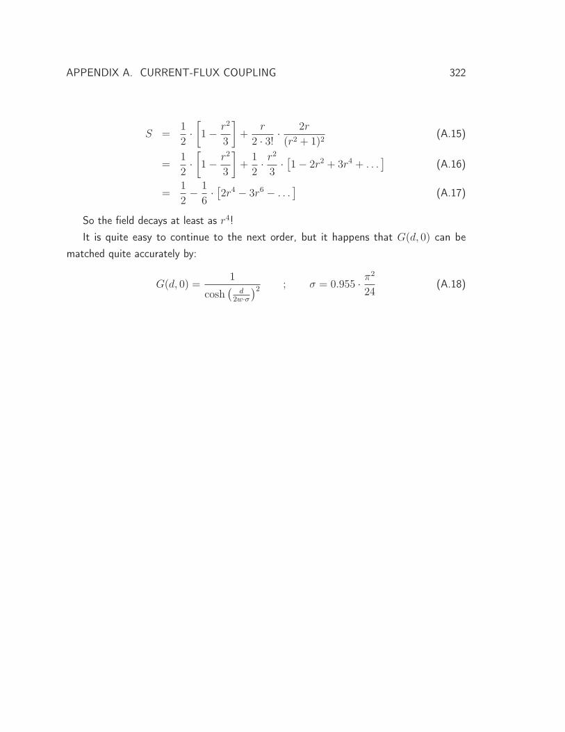
APPENDIX A. CURRENT-FLUX COUPLING 322
S =1
2·[1 − r2
3
]+
r
2 · 3! ·2r
(r2 + 1)2(A.15)
=1
2·[1 − r2
3
]+
1
2· r
2
3· [1 − 2r2 + 3r4 + . . .
](A.16)
=1
2− 1
6· [2r4 − 3r6 − . . .
](A.17)
So the field decays at least as r4!It is quite easy to continue to the next order, but it happens that G(d, 0) can be
matched quite accurately by:
G(d, 0) =1
cosh(
d2w·σ
)2 ; σ = 0.955 · π2
24(A.18)

APPENDIX A. CURRENT-FLUX COUPLING 323
This is OK, but not exactly what I need. I want to see what is the coupling due to afinite segment of current. To do so, I will calculate the flux threading a square of width w
and height h positioned d away from a current segment of length L. I will assume thatthe segment lies on the x-axis.
I start from Biot Savart Lew:
B =
∫μ0I
4π
�dl × �r
|r|3
First, I calculate the field at position (x, y) due to the current segment:
B(x, y) =μ0I
4π
L/2∫−L/2
�dl × �r
|r|3 (A.19)
=μ0Iz
4π
L/2∫−L/2
y
((x − l)2 + y2)3/2dl = ⊗ (A.20)
�r stands for (x, y) − (l, 0) = (x − l, y), and �dl is simply (dl, 0). Hence:

APPENDIX A. CURRENT-FLUX COUPLING 324
By using x − l = y tan θ, this integral is transformed to be:
⊗ =μ0Iz
4πy
arctan( 2x+Ly )∫
arctan( 2x−Ly )
cos θdθ (A.21)
=μ0Iz
4πy
[sin
(arctan
(2x+ L
y
))− sin
(arctan
(2x − L
y
))](A.22)
=μ0Iz
4πy
⎡⎣ L2− x√(
L2− x
)2+ y2
+L2+ x√(
L2+ x
)2+ y2
⎤⎦ (A.23)
For a point very close to the segment, y � L2− x, L
2+ x, this expression reduces to:
μ0Iz
2πy
Which is the field due to infinite current line.The next step is to integrate this field within the area of the squid:
Φ =
D+H∫D
dy
W2∫
−W2
dxB(x, y) (A.24)
=μ0I
4π
D+H∫D
dy
y
W2∫
−W2
⎡⎣ L2− x√(
L2− x
)2+ y2
+L2+ x√(
L2+ x
)2+ y2
⎤⎦ dx (A.25)
=μ0I
2π
D+H∫D
dy
y
W2∫
−W2
L2+ x√(
L2+ x
)2+ y2
dx (A.26)
=μ0I
2π
D+H∫D
dy
y
⎡⎣√(L
2+ x
)2
+ y2
⎤⎦∣∣∣∣∣∣W2
−W2
(A.27)
=μ0I
2π
D+H∫D
dy
y
⎡⎣√(L+W
2
)2
+ y2 −√(
L − W
2
)2
+ y2
⎤⎦ = ⊕ (A.28)
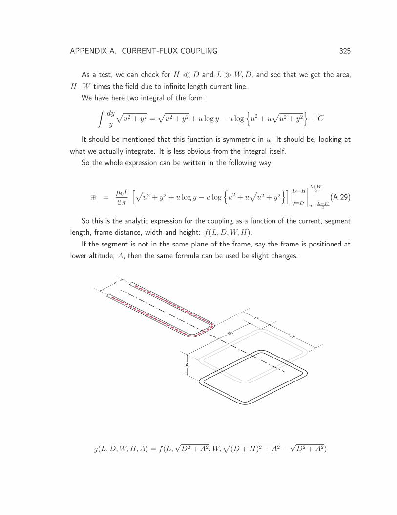
APPENDIX A. CURRENT-FLUX COUPLING 325
As a test, we can check for H � D and L � W,D, and see that we get the area,H · W times the field due to infinite length current line.
We have here two integral of the form:∫dy
y
√u2 + y2 =
√u2 + y2 + u log y − u log
{u2 + u
√u2 + y2
}+ C
It should be mentioned that this function is symmetric in u. It should be, looking atwhat we actually integrate. It is less obvious from the integral itself.
So the whole expression can be written in the following way:
⊕ =μ0I
2π
[√u2 + y2 + u log y − u log
{u2 + u
√u2 + y2
}]∣∣∣D+H
y=D
∣∣∣∣L+W2
u=L−W2
(A.29)
So this is the analytic expression for the coupling as a function of the current, segmentlength, frame distance, width and height: f(L,D,W,H).
If the segment is not in the same plane of the frame, say the frame is positioned atlower altitude, A, then the same formula can be used be slight changes:
g(L,D,W,H,A) = f(L,√D2 + A2,W,
√(D +H)2 + A2 −
√D2 + A2)
APPENDIX A. CURRENT-FLUX COUPLING 326
We can also calculate the flux coupling when the frame is not sitting symmetric relativeto the current segment, say with some offset O:
If W < 2 ∗ O, then:
h(L,D,W,H,O) =1
2[f(L,D,W + 2O,H) + f(L,D,W − 2O,H)]
Otherwise:
h(L,D,W,H,O) =1
2[f(L,D,W + 2O,H) − f(L,D, 2O − W,H)]
.And, of course, we can combine the offset and the altitude together.This will be useful if we want to take into account the image currents cause by the SC
box. As long as the dimensions are of the order of the width and height of the cavity, wecan take the main term alone. For example, a frame of 100 μm by 100 μm located 400 μm
away from a 500 μm current segment carrying 1mA has one flux quantum threading it.For the same parameters, the first image caused by the top SC plane, assuming the cavityis 1mm high, gives 8% of the flux. We have to of these, so taking the first term only hasan error no more than 16% (we have two such images). The error due to the images causeby the side SC planes of the order of 9%, so the total error is of the order of 35%. Wecan still get half a flux out of the same current.
APPENDIX B
Mathematica Code
Here we reproduce the Mathematica code used for state and process tomography andsimulating AllXY syndromes. This code can be used to convert experimental state
tomograms into a χ process matrix, or to simulate the matrix of an ideal process. Thiscode works only for two qubits (section 7.4), but can be easily generalized for any number.However, in practice, Mathematica is too slow to operate on more than two qubits, so thecode was re-written in Matlab for the process tomography of section 8.1.6. That code isnot included here, but is functionally identical.
We also calculate the error syndromes of AllXY both analytically and in comparisonwith data. Since this code was written, a much better method has been developed usingthe QuTiP package for Python∗. We include this code so that the plots from section 5.2.3can be easily reproduced, but going forward it would be wise to port the code over toPython.
∗ https://code.google.com/p/qutip/
327
DefinitonsWe begin by defining our language, including raising and lowering operators, dagger, tensor product, and Pauli operators. We then make functions to create and manipulate single-qubit states, which generalize to two qubits. We also define a function to produce a Pauli tomogram from a density matrix and Β and Κ matrices for converting state tomograms into Χ process matrices.
In[1]:=
Needs�"BarCharts`"�
ident�dim_� :�SparseArray���Poutine$_, Poutine$_� �� 1�, �dim, dim��;
destroy�dim_� :� SparseArray��Poutine$_, Maudite$_� �;Poutine$ � 1 �� Maudite$ �� Sqrt�Poutine$�, �dim, dim��;
dagger�a_� :� ConjugateTranspose�a�;��Transpose�Conjugate�a��; ��
TensProd�a_, b_� :� SparseArray�KroneckerProduct�a, b��;
General::obspkg :BarCharts` is now obsolete. The legacy version being loaded may conflict with current
Mathematica functionality. See the Compatibility Guide for updating information.
APPENDIX B. MATHEMATICA CODE 328
In[6]:= Σp � destroy�2�;Σm � dagger�Σp�;Σx � Σp � Σm;Σy � �1 � ��� Σp � � Σm�; �� ��� ��Σz � � Σm.Σp � Σp.Σm;Σi � ident�2�;
Σii � TensProd�Σi, Σi�;Σxi � TensProd�Σx, Σi�;Σyi � TensProd�Σy, Σi�;Σzi � TensProd�Σz, Σi�;
Σix � TensProd�Σi, Σx�;Σxx � TensProd�Σx, Σx�;Σyx � TensProd�Σy, Σx�;Σzx � TensProd�Σz, Σx�;
Σiy � TensProd�Σi, Σy�;Σxy � TensProd�Σx, Σy�;Σyy � TensProd�Σy, Σy�;Σzy � TensProd�Σz, Σy�;
Σiz � TensProd�Σi, Σz�;Σxz � TensProd�Σx, Σz�;Σyz � TensProd�Σy, Σz�;Σzz � TensProd�Σz, Σz�;
DistributeDefinitions�Σx, Σy, Σz, Σi, Σii, Σxi, Σyi, Σzi,Σix, Σxx, Σyx, Σzx, Σiy, Σxy, Σyy, Σzy, Σiz, Σxz, Σyz, Σzz�;
U�Θ_, Σ_� :� MatrixExp��Θ
2Normal�Σ�;
In[30]:= �� Make a one qubit density matrix with QId,X90p, Y90p, or Xp rotations on the qubits ��makeΡ1�state_� :� Module��o1�,Ρ � �Σi � Σz� � 2; �� start from the ground state ��
o1 � Switch�Characters�state���1��,"I", U�0, Σi�,"X", U�Π � 2, Σx�,"Y", U�Π � 2, Σy�,"Z", U�Π, Σx�,_, U�0, Σi��;
Return�dagger�o1�.Ρ.o1�;�;
�� Get Pauli correlations from density matrix ��paulitomo1�Ρ_� :� �Tr�Ρ.Σi�, Tr�Ρ.Σx�, Tr�Ρ.Σy�, Tr�Ρ.Σz�� � 2;
APPENDIX B. MATHEMATICA CODE 329
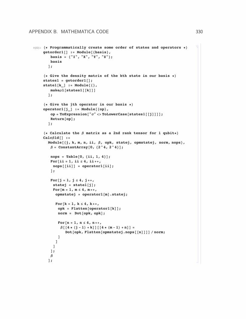
In[32]:= �� Programmatically create some order of states and operators ��getorder1�� :� Module��basis�,
basis � �"I", "X", "Y", "Z"�;basis�;
�� Give the density matrix of the kth state in our basis ��states1 � getorder1��;state1�k_� :� Module���,
makeΡ1�states1��k����;
�� Give the jth operator in our basis ��operator1�j_� :� Module��op�,
op � ToExpression�"Σ" �� ToLowerCase�states1��j����;Return�op�;�;
�� Calculate the Β matrix as a 2nd rank tensor for 1 qubit��CalcΒ1d�� :�
Module��j, k, m, n, ii, Β, opk, statej, opmstatej, norm, nops�,Β � ConstantArray�0, �2^4, 2^4��;
nops � Table�0, �ii, 1, 4��;For�ii � 1, ii � 4, ii��,nops��ii�� � operator1�ii�;�;
For�j � 1, j � 4, j��,statej � state1�j�;For�m � 1, m � 4, m��,opmstatej � operator1�m�.statej;
For�k � 1, k � 4, k��,opk � Flatten�operator1�k��;norm � Dot�opk, opk�;
For�n � 1, n � 4, n��,��4 � �j � 1� � k����4 � �m � 1� � n�� �
Dot�opk, Flatten�opmstatej.nops��n���� � norm;����;�;
APPENDIX B. MATHEMATICA CODE 330
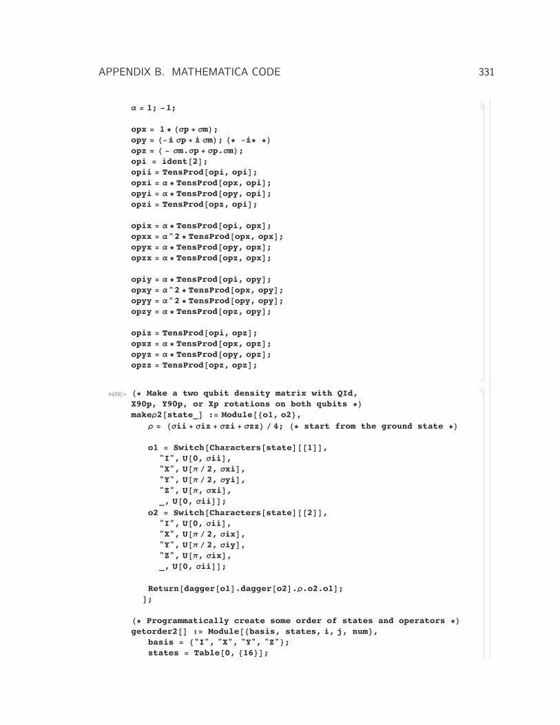
Α � 1; �1;
opx � 1 � �Σp � Σm�;opy � ��� Σp � � Σm�; �� ��� ��opz � � � Σm.Σp � Σp.Σm�;opi � ident�2�;opii � TensProd�opi, opi�;opxi � Α � TensProd�opx, opi�;opyi � Α � TensProd�opy, opi�;opzi � TensProd�opz, opi�;
opix � Α � TensProd�opi, opx�;opxx � Α^2 � TensProd�opx, opx�;opyx � Α � TensProd�opy, opx�;opzx � Α � TensProd�opz, opx�;
opiy � Α � TensProd�opi, opy�;opxy � Α^2 � TensProd�opx, opy�;opyy � Α^2 � TensProd�opy, opy�;opzy � Α � TensProd�opz, opy�;
opiz � TensProd�opi, opz�;opxz � Α � TensProd�opx, opz�;opyz � Α � TensProd�opy, opz�;opzz � TensProd�opz, opz�;
In[59]:= �� Make a two qubit density matrix with QId,X90p, Y90p, or Xp rotations on both qubits ��makeΡ2�state_� :� Module��o1, o2�,Ρ � �Σii � Σiz � Σzi � Σzz� � 4; �� start from the ground state ��
o1 � Switch�Characters�state���1��,"I", U�0, Σii�,"X", U�Π � 2, Σxi�,"Y", U�Π � 2, Σyi�,"Z", U�Π, Σxi�,_, U�0, Σii��;
o2 � Switch�Characters�state���2��,"I", U�0, Σii�,"X", U�Π � 2, Σix�,"Y", U�Π � 2, Σiy�,"Z", U�Π, Σix�,_, U�0, Σii��;
Return�dagger�o1�.dagger�o2�.Ρ.o2.o1�;�;
�� Programmatically create some order of states and operators ��getorder2�� :� Module��basis, states, i, j, num�,
basis � �"I", "X", "Y", "Z"�;states � Table�0, �16��;
APPENDIX B. MATHEMATICA CODE 331

�� First programmatically create some order of states ��num � 1;For�i � 1, i � Length�basis�, i��,For�j � 1, j �� Length�basis�, j��,states��num�� � basis��i�� �� basis��j��;num��;��;states�;
states2 � getorder2��;�� Give the density matrix of the kth state in our basis ��state2�k_� :� Module���,��states � getorder2��;��makeΡ2�states2��k����;
�� Give the jth operator in our basis ��operator2�j_� :� Module���,��states � getorder2��;ToExpression�"Σ"��ToLowerCase�states2��j������ToExpression�"op" �� ToLowerCase�states2��j�����;
��Ρ2�xi_,yi_,zi_,ix_,iy_,iz_,xy_,xz_,yx_,yz_,zx_,zy_,xx_,yy_,zz_� :��Σii�xi�Σxi�yi�Σyi�zi�Σzi�ix�Σix�xx�Σxx�yx�Σyz�zx�Σzx�iy�Σiy�
xy�Σxy�yy�Σyy�zy�Σzy�iz�Σiz�xz�Σxz�yz�Σyz�zz�Σzz�;��
paulitomo2�Ρ_� :� Table�Tr�Ρ.operator2�ii��, �ii, 1, 16�� � 4;
get2QΛs�fullΛ_� :� Module��Α�,Λ � Table�0, �16��;
Α � �1;
Λ��1�� � fullΛ��1��; �� II ��Λ��2�� � Α � fullΛ��5��; �� IX ��Λ��3�� � Α � fullΛ��6��; �� IY ��Λ��4�� � fullΛ��7��; �� IZ ��Λ��5�� � Α � fullΛ��2��; �� XI ��Λ��6�� � fullΛ��11��; �� XX ��Λ��7�� � fullΛ��12��; �� XY ��Λ��8�� � Α � fullΛ��13��; �� XZ ��Λ��9�� � Α � fullΛ��3��; �� YI ��Λ��10�� � fullΛ��14��; �� YX ��Λ��11�� � fullΛ��15��; �� YY ��Λ��12�� � Α � fullΛ��16��; �� YZ ��Λ��13�� � fullΛ��4��; �� ZI ��Λ��14�� � Α � fullΛ��17��; �� ZX ��
APPENDIX B. MATHEMATICA CODE 332
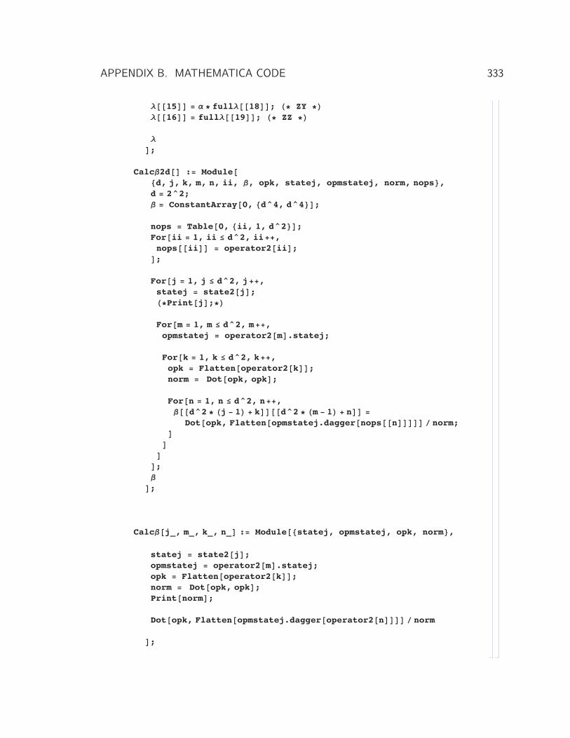
Λ��15�� � Α � fullΛ��18��; �� ZY ��Λ��16�� � fullΛ��19��; �� ZZ ��
Λ�;
CalcΒ2d�� :� Module��d, j, k, m, n, ii, Β, opk, statej, opmstatej, norm, nops�,d � 2^2;Β � ConstantArray�0, �d^4, d^4��;
nops � Table�0, �ii, 1, d^2��;For�ii � 1, ii � d^2, ii��,nops��ii�� � operator2�ii�;�;
For�j � 1, j � d^2, j��,statej � state2�j�;��Print�j�;��
For�m � 1, m � d^2, m��,opmstatej � operator2�m�.statej;
For�k � 1, k � d^2, k��,opk � Flatten�operator2�k��;norm � Dot�opk, opk�;
For�n � 1, n � d^2, n��,��d^2 � �j � 1� � k����d^2 � �m � 1� � n�� �
Dot�opk, Flatten�opmstatej.dagger�nops��n����� � norm;����;�;
Calc�j_, m_, k_, n_� :� Module��statej, opmstatej, opk, norm�,
statej � state2�j�;opmstatej � operator2�m�.statej;opk � Flatten�operator2�k��;norm � Dot�opk, opk�;Print�norm�;
Dot�opk, Flatten�opmstatej.dagger�operator2�n���� � norm
�;
APPENDIX B. MATHEMATICA CODE 333
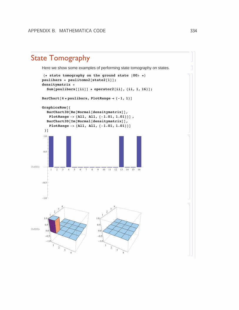
State TomographyHere we show some examples of performing state tomography on states.
�� state tomography on the ground state 00� ��paulibars � paulitomo2�state2�1��;densitymatrix �
Sum�paulibars��ii�� � operator2�ii�, �ii, 1, 16��;
BarChart�4 � paulibars, PlotRange � ��1, 1��
GraphicsRow��BarChart3D�Re�Normal�densitymatrix��,PlotRange �� �All, All, ��1.01, 1.01��� ,
BarChart3D�Im�Normal�densitymatrix��,PlotRange �� �All, All, ��1.01, 1.01���
��
Out[92]=1 2 3 4 5 6 7 8 9 10 11 12 13 14 15 16
�1.0
�0.5
0.5
1.0
Out[93]=
12
34
12
34
�1.0
�0.5
0.0
0.5
1.0
12
34
12
34
�1.0
�0.5
0.0
0.5
1.0
APPENDIX B. MATHEMATICA CODE 334
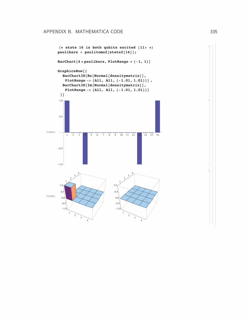
�� state 16 is both qubits excited 11� ��paulibars � paulitomo2�state2�16��;
BarChart�4 � paulibars, PlotRange � ��1, 1��
GraphicsRow��BarChart3D�Re�Normal�densitymatrix��,PlotRange �� �All, All, ��1.01, 1.01��� ,
BarChart3D�Im�Normal�densitymatrix��,PlotRange �� �All, All, ��1.01, 1.01���
��
Out[95]=1 2 3 4 5 6 7 8 9 10 11 12 13 14 15 16
�1.0
�0.5
0.5
1.0
Out[96]=
12
34
12
34
�1.0
�0.5
0.0
0.5
1.0
12
34
12
34
�1.0
�0.5
0.0
0.5
1.0
APPENDIX B. MATHEMATICA CODE 335
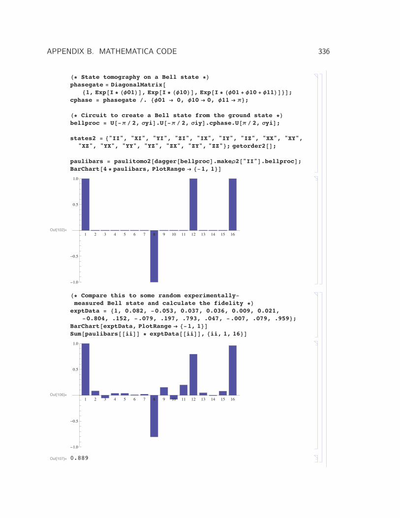
�� State tomography on a Bell state ��phasegate � DiagonalMatrix��1, Exp�I � �Φ01��, Exp�I � �Φ10��, Exp�I � �Φ01 � Φ10 � Φ11����;
cphase � phasegate �. �Φ01 � 0, Φ10 � 0, Φ11 � Π�;
�� Circuit to create a Bell state from the ground state ��bellproc � U��Π � 2, Σyi�.U��Π � 2, Σiy�.cphase.U�Π � 2, Σyi�;
states2 � �"II", "XI", "YI", "ZI", "IX", "IY", "IZ", "XX", "XY","XZ", "YX", "YY", "YZ", "ZX", "ZY", "ZZ"�; getorder2��;
paulibars � paulitomo2�dagger�bellproc�.makeΡ2�"II"�.bellproc�;BarChart�4 � paulibars, PlotRange � ��1, 1��
Out[102]=1 2 3 4 5 6 7 8 9 10 11 12 13 14 15 16
�1.0
�0.5
0.5
1.0
�� Compare this to some random experimentally�measured Bell state and calculate the fidelity ��
exptData � �1, 0.082, �0.053, 0.037, 0.036, 0.009, 0.021,�0.804, .152, �.079, .197, .793, .047, �.007, .079, .959�;
BarChart�exptData, PlotRange � ��1, 1��Sum�paulibars��ii�� � exptData��ii��, �ii, 1, 16��
Out[106]=1 2 3 4 5 6 7 8 9 10 11 12 13 14 15 16
�1.0
�0.5
0.5
1.0
Out[107]= 0.889
APPENDIX B. MATHEMATICA CODE 336
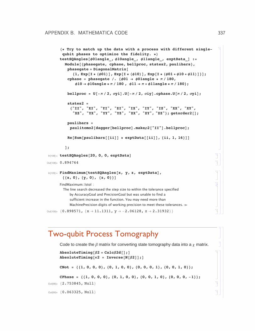
�� Try to match up the data with a process with different single�qubit phases to optimize the fidelity. ��
testSQAngles�Φ01angle_, Φ10angle_, Φ11angle_, exptData_� :�Module��phasegate, cphase, bellproc, states2, paulibars�,phasegate � DiagonalMatrix��1, Exp�I � �Φ01��, Exp�I � �Φ10��, Exp�I � �Φ01 � Φ10 � Φ11����;
cphase � phasegate �. �Φ01 � Φ01angle � Π � 180,Φ10 � Φ10angle � Π � 180 , Φ11 � Π � Φ11angle � Π � 180�;
bellproc � U��Π � 2, Σyi�.U��Π � 2, Σiy�.cphase.U�Π � 2, Σyi�;
states2 ��"II", "XI", "YI", "ZI", "IX", "IY", "IZ", "XX", "XY","XZ", "YX", "YY", "YZ", "ZX", "ZY", "ZZ"�; getorder2��;
paulibars �paulitomo2�dagger�bellproc�.makeΡ2�"II"�.bellproc�;
Re�Sum�paulibars��ii�� � exptData��ii��, �ii, 1, 16���
�;In[108]:= testSQAngles�20, 0, 0, exptData�Out[108]= 0.894764
In[109]:= FindMaximum�testSQAngles�x, y, z, exptData�,��x, 0�, �y, 0�, �z, 0���
FindMaximum::lstol :The line search decreased the step size to within the tolerance specified
by AccuracyGoal and PrecisionGoal but was unable to find asufficient increase in the function. You may need more than MachinePrecision digits of working precision to meet these tolerances. �
Out[109]= �0.898571, �x � 11.1311, y � �2.06128, z � 2.31932��
Two-qubit Process TomographyCode to create the Β matrix for converting state tomography data into a Χ matrix.
AbsoluteTiming�Β2 � CalcΒ2d��;�AbsoluteTiming�Κ2 � Inverse�N�Β2��;�
CNot � ��1, 0, 0, 0�, �0, 1, 0, 0�, �0, 0, 0, 1�, �0, 0, 1, 0��;
CPhase � ��1, 0, 0, 0�, �0, 1, 0, 0�, �0, 0, 1, 0�, �0, 0, 0, �1��;Out[68]= �2.753845, Null�
Out[69]= �0.063325, Null�
APPENDIX B. MATHEMATICA CODE 337
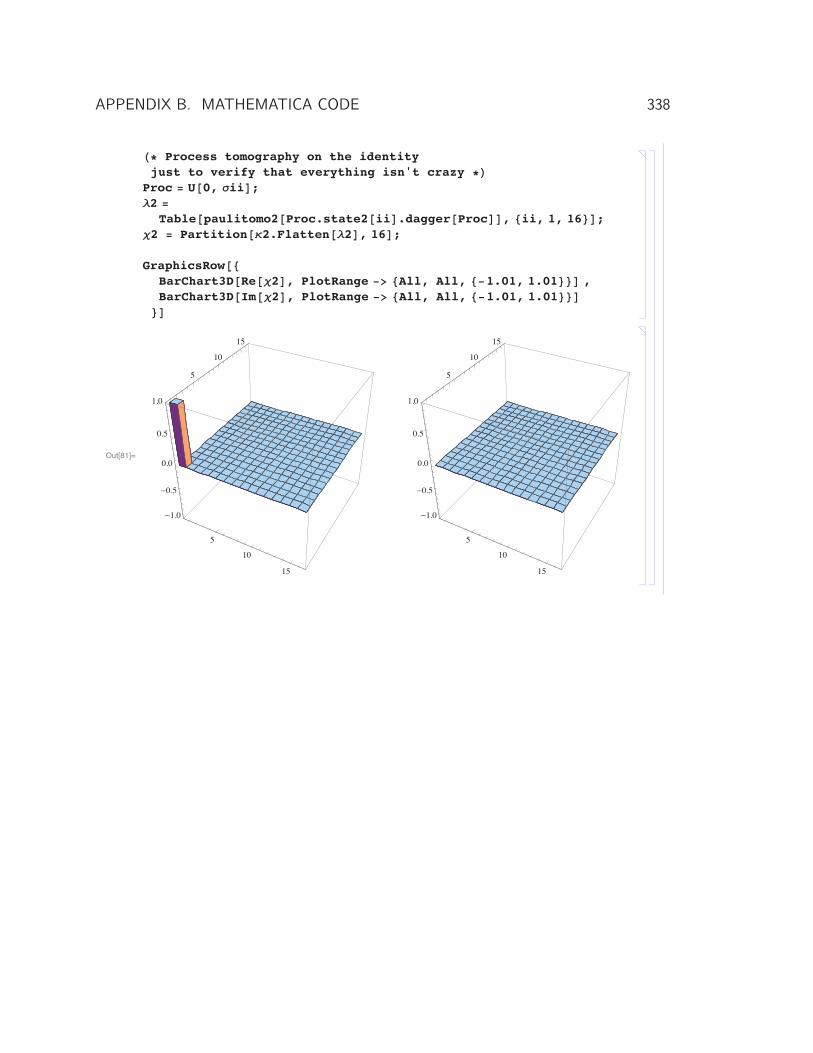
�� Process tomography on the identityjust to verify that everything isn't crazy ��
Proc � U�0, Σii�;Λ2 �
Table�paulitomo2�Proc.state2�ii�.dagger�Proc��, �ii, 1, 16��;Χ2 � Partition�Κ2.Flatten�Λ2�, 16�;
GraphicsRow��BarChart3D�Re�Χ2�, PlotRange �� �All, All, ��1.01, 1.01��� ,BarChart3D�Im�Χ2�, PlotRange �� �All, All, ��1.01, 1.01�����
Out[81]=
5
10
15
5
10
15
�1.0
�0.5
0.0
0.5
1.0
5
10
15
5
10
15
�1.0
�0.5
0.0
0.5
1.0
APPENDIX B. MATHEMATICA CODE 338

�� Proc tomo on the cNOT gate ��Proc � CNot;Λ2 �
Table�paulitomo2�Proc.state2�ii�.dagger�Proc��, �ii, 1, 16��;Χ2 � Partition�Κ2.Flatten�Λ2�, 16�;��Χ2 ��MatrixForm��
GraphicsRow��BarChart3D�Re�Χ2�, PlotRange �� �All, All, ��0.251, 0.251��� ,BarChart3D�Im�Χ2�, PlotRange �� �All, All, ��0.251, 0.251�����
Out[77]=
5
10
15
5
10
15
�0.2
0.0
0.2
5
10
15
5
10
15
�0.2
0.0
0.2
APPENDIX B. MATHEMATICA CODE 339
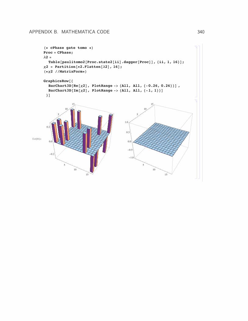
�� cPhase gate tomo ��Proc � CPhase;Λ2 �
Table�paulitomo2�Proc.state2�ii�.dagger�Proc��, �ii, 1, 16��;Χ2 � Partition�Κ2.Flatten�Λ2�, 16�;��Χ2 ��MatrixForm��
GraphicsRow��BarChart3D�Re�Χ2�, PlotRange �� �All, All, ��0.26, 0.26��� ,BarChart3D�Im�Χ2�, PlotRange �� �All, All, ��1, 1�����
Out[85]=
5
10
15
5
10
15
�0.2
0.0
0.2
5
10
15
5
10
15
�1.0
�0.5
0.0
0.5
1.0
APPENDIX B. MATHEMATICA CODE 340
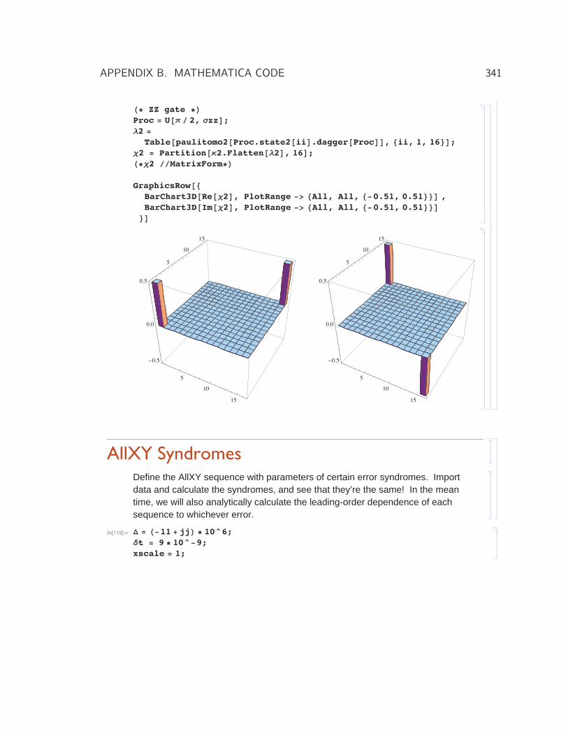
�� ZZ gate ��Proc � U�Π � 2, Σzz�;Λ2 �
Table�paulitomo2�Proc.state2�ii�.dagger�Proc��, �ii, 1, 16��;Χ2 � Partition�Κ2.Flatten�Λ2�, 16�;��Χ2 ��MatrixForm��
GraphicsRow��BarChart3D�Re�Χ2�, PlotRange �� �All, All, ��0.51, 0.51��� ,BarChart3D�Im�Χ2�, PlotRange �� �All, All, ��0.51, 0.51�����
5
10
15
5
10
15
�0.5
0.0
0.5
5
10
15
5
10
15
�0.5
0.0
0.5
AllXY SyndromesDefine the AllXY sequence with parameters of certain error syndromes. Import data and calculate the syndromes, and see that they’re the same! In the mean time, we will also analytically calculate the leading-order dependence of each sequence to whichever error.
In[119]:= � � ��11 � jj� � 10^6;Δt � 9 � 10^�9;xscale � 1;
APPENDIX B. MATHEMATICA CODE 341

In[117]:= zProj�operator_� :� Tr�operator.state1�1�.dagger�operator�.Σz�;
GetAllXY�rs_, �_, Δt_, xscale_� :� Module���,
�op � �2 Π � � � Δt � Σz;
��U�Π, Σi � �op � Π�, U�Π, Σi � �op � Π��,�U�Π, rs � xscale � Σx � �op � Π�, U�Π, rs � xscale � Σx � �op � Π��,�U�Π, rs � Σy � �op � Π�, U�Π, rs � Σy � �op � Π��,�U�Π, rs � xscale � Σx � �op � Π�, U�Π, rs � Σy � �op � Π��,�U�Π, rs � Σy � �op � Π�, U�Π, rs � xscale � Σx � �op � Π��,
�U�Π � 2, rs � xscale � Σx � �op � �Π � 2��, U�Π, Σi � �op � Π��,�U�Π � 2, rs � Σy � �op � �Π � 2��, U�Π, Σi � �op � Π��,�U�Π � 2, rs � xscale � Σx � �op � �Π � 2��,U�Π � 2, rs � Σy � �op � �Π � 2���, �U�Π � 2, rs � Σy � �op � �Π � 2��,U�Π � 2, rs � xscale � Σx � �op � �Π � 2���,�U�Π � 2, rs � xscale � Σx � �op � �Π � 2��, U�Π, rs � Σy � �op � Π��,�U�Π � 2, rs � Σy � �op � �Π � 2��, U�Π, rs � xscale � Σx � �op � Π��,
�U�Π, rs � xscale � Σx � �op � Π�, U�Π � 2, rs � Σy � �op � �Π � 2���,�U�Π, rs � Σy � �op � Π�, U�Π � 2, rs � xscale � Σx � �op � �Π � 2���,
�U�Π � 2, rs � xscale � Σx � �op � �Π � 2��,U�Π, rs � xscale � Σx � �op � Π��, �U�Π, rs � xscale � Σx � �op � Π�,U�Π � 2, rs � xscale � Σx � �op � �Π � 2���,�U�Π � 2, rs � Σy � �op � �Π � 2��, U�Π, rs � Σy � �op � Π��,�U�Π, rs � Σy � �op � Π�, U�Π � 2, rs � Σy � �op � �Π � 2���,
�U�Π, rs � Σy � �op � Π�, U�Π, Σi � �op � Π��,�U�Π, rs � Σy � �op � Π�, U�Π, Σi � �op � Π��,�U�Π � 2, rs � xscale � Σx � �op � �Π � 2��,U�Π � 2, rs � xscale � Σx � �op � �Π � 2���,�U�Π � 2, rs � Σy � �op � �Π � 2��, U�Π � 2, rs � Σy � �op � �Π � 2�����;
APPENDIX B. MATHEMATICA CODE 342
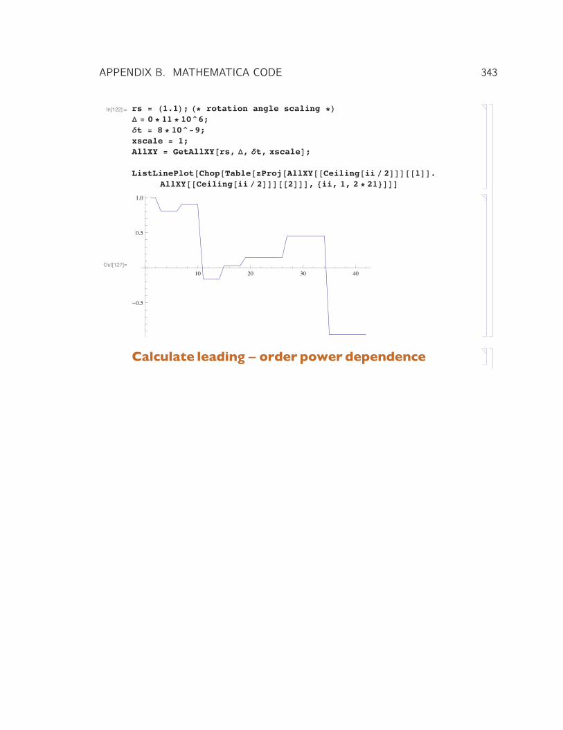
In[122]:= rs � �1.1�; �� rotation angle scaling ��� � 0 � 11 � 10^6;Δt � 8 � 10^�9;xscale � 1;AllXY � GetAllXY�rs, �, Δt, xscale�;
ListLinePlot�Chop�Table�zProj�AllXY��Ceiling�ii � 2�����1��.AllXY��Ceiling�ii � 2�����2���, �ii, 1, 2 � 21����
Out[127]=
10 20 30 40
�0.5
0.5
1.0
Calculate leading � order power dependence
APPENDIX B. MATHEMATICA CODE 343
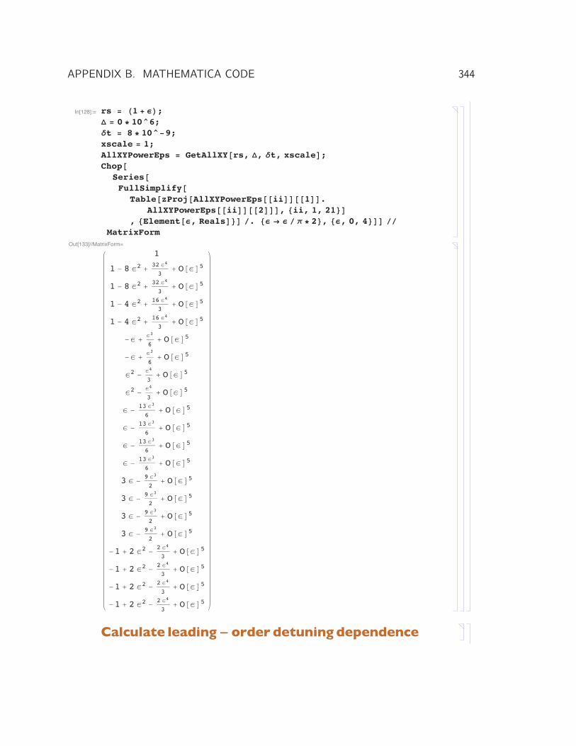
In[128]:= rs � �1 � Ε�;� � 0 � 10^6;Δt � 8 � 10^�9;xscale � 1;AllXYPowerEps � GetAllXY�rs, �, Δt, xscale�;Chop�
Series�FullSimplify�
Table�zProj�AllXYPowerEps��ii����1��.AllXYPowerEps��ii����2���, �ii, 1, 21��
, �Element�Ε, Reals��� �. �Ε � Ε � Π � 2�, �Ε, 0, 4��� ��MatrixForm
Out[133]//MatrixForm=
1
1 � 8 Ε2 � 32 Ε4
3� O�Ε�5
1 � 8 Ε2 � 32 Ε4
3� O�Ε�5
1 � 4 Ε2 � 16 Ε4
3� O�Ε�5
1 � 4 Ε2 � 16 Ε4
3� O�Ε�5
�Ε � Ε3
6� O�Ε�5
�Ε � Ε3
6� O�Ε�5
Ε2 � Ε4
3� O�Ε�5
Ε2 � Ε4
3� O�Ε�5
Ε � 13 Ε3
6� O�Ε�5
Ε � 13 Ε3
6� O�Ε�5
Ε � 13 Ε3
6� O�Ε�5
Ε � 13 Ε3
6� O�Ε�5
3 Ε � 9 Ε3
2� O�Ε�5
3 Ε � 9 Ε3
2� O�Ε�5
3 Ε � 9 Ε3
2� O�Ε�5
3 Ε � 9 Ε3
2� O�Ε�5
�1 � 2 Ε2 � 2 Ε4
3� O�Ε�5
�1 � 2 Ε2 � 2 Ε4
3� O�Ε�5
�1 � 2 Ε2 � 2 Ε4
3� O�Ε�5
�1 � 2 Ε2 � 2 Ε4
3� O�Ε�5
Calculate leading � order detuning dependence
APPENDIX B. MATHEMATICA CODE 344
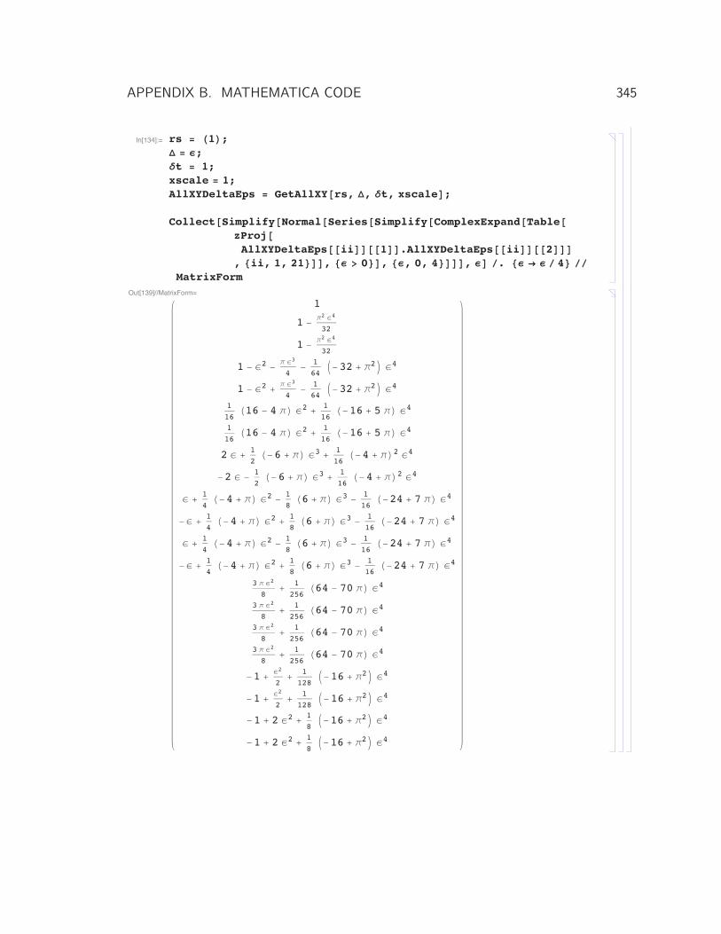
In[134]:= rs � �1�;� � Ε;Δt � 1;xscale � 1;AllXYDeltaEps � GetAllXY�rs, �, Δt, xscale�;
Collect�Simplify�Normal�Series�Simplify�ComplexExpand�Table�zProj�AllXYDeltaEps��ii����1��.AllXYDeltaEps��ii����2���
, �ii, 1, 21���, �Ε � 0��, �Ε, 0, 4����, Ε� �. �Ε � Ε � 4� ��MatrixForm
Out[139]//MatrixForm=
1
1 � Π2 Ε4
32
1 � Π2 Ε4
32
1 � Ε2 � Π Ε3
4� 1
64��32 � Π2� Ε4
1 � Ε2 � Π Ε3
4� 1
64��32 � Π2� Ε4
1
16�16 � 4 Π Ε2 � 1
16��16 � 5 Π Ε4
1
16�16 � 4 Π Ε2 � 1
16��16 � 5 Π Ε4
2 Ε � 1
2��6 � Π Ε3 � 1
16��4 � Π2 Ε4
�2 Ε � 1
2��6 � Π Ε3 � 1
16��4 � Π2 Ε4
Ε � 1
4��4 � Π Ε2 � 1
8�6 � Π Ε3 � 1
16��24 � 7 Π Ε4
�Ε � 1
4��4 � Π Ε2 � 1
8�6 � Π Ε3 � 1
16��24 � 7 Π Ε4
Ε � 1
4��4 � Π Ε2 � 1
8�6 � Π Ε3 � 1
16��24 � 7 Π Ε4
�Ε � 1
4��4 � Π Ε2 � 1
8�6 � Π Ε3 � 1
16��24 � 7 Π Ε4
3 Π Ε2
8� 1
256�64 � 70 Π Ε4
3 Π Ε2
8� 1
256�64 � 70 Π Ε4
3 Π Ε2
8� 1
256�64 � 70 Π Ε4
3 Π Ε2
8� 1
256�64 � 70 Π Ε4
�1 � Ε2
2� 1
128��16 � Π2� Ε4
�1 � Ε2
2� 1
128��16 � Π2� Ε4
�1 � 2 Ε2 � 1
8��16 � Π2� Ε4
�1 � 2 Ε2 � 1
8��16 � Π2� Ε4
APPENDIX B. MATHEMATICA CODE 345
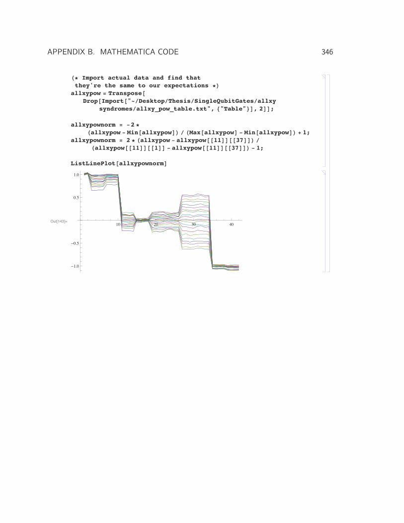
�� Import actual data and find thatthey're the same to our expectations ��
allxypow � Transpose�Drop�Import�"��Desktop�Thesis�SingleQubitGates�allxy
syndromes�allxy_pow_table.txt", �"Table"��, 2��;
allxypownorm � �2 ��allxypow � Min�allxypow�� � �Max�allxypow� � Min�allxypow�� � 1;
allxypownorm � 2 � �allxypow � allxypow��11����37��� ��allxypow��11����1�� � allxypow��11����37��� � 1;
ListLinePlot�allxypownorm�
Out[143]=10 20 30 40
�1.0
�0.5
0.5
1.0
APPENDIX B. MATHEMATICA CODE 346
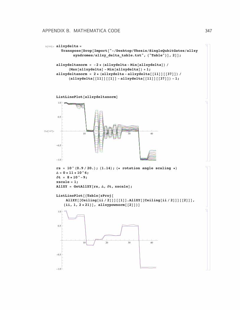
In[144]:= allxydelta �Transpose�Drop�Import�"��Desktop�Thesis�SingleQubitGates�allxy
syndromes�allxy_delta_table.txt", �"Table"��, 2��;
allxydeltanorm � �2 � �allxydelta � Min�allxydelta�� ��Max�allxydelta� � Min�allxydelta�� � 1;
allxydeltanorm � 2 � �allxydelta � allxydelta��11����37��� ��allxydelta��11����1�� � allxydelta��11����37��� � 1;
ListLinePlot�allxydeltanorm�
Out[147]=10 20 30 40
�1.0
�0.5
0.5
1.0
rs � 10^�0.9 � 20.�; �1.14�; �� rotation angle scaling ��� � 0 � 11 � 10^6;Δt � 8 � 10^�9;xscale � 1;AllXY � GetAllXY�rs, �, Δt, xscale�;
ListLinePlot��Table�zProj�AllXY��Ceiling�ii � 2�����1��.AllXY��Ceiling�ii � 2�����2���,�ii, 1, 2 � 21��, allxypownorm��2����
10 20 30 40
�1.0
�0.5
0.5
1.0
APPENDIX B. MATHEMATICA CODE 347
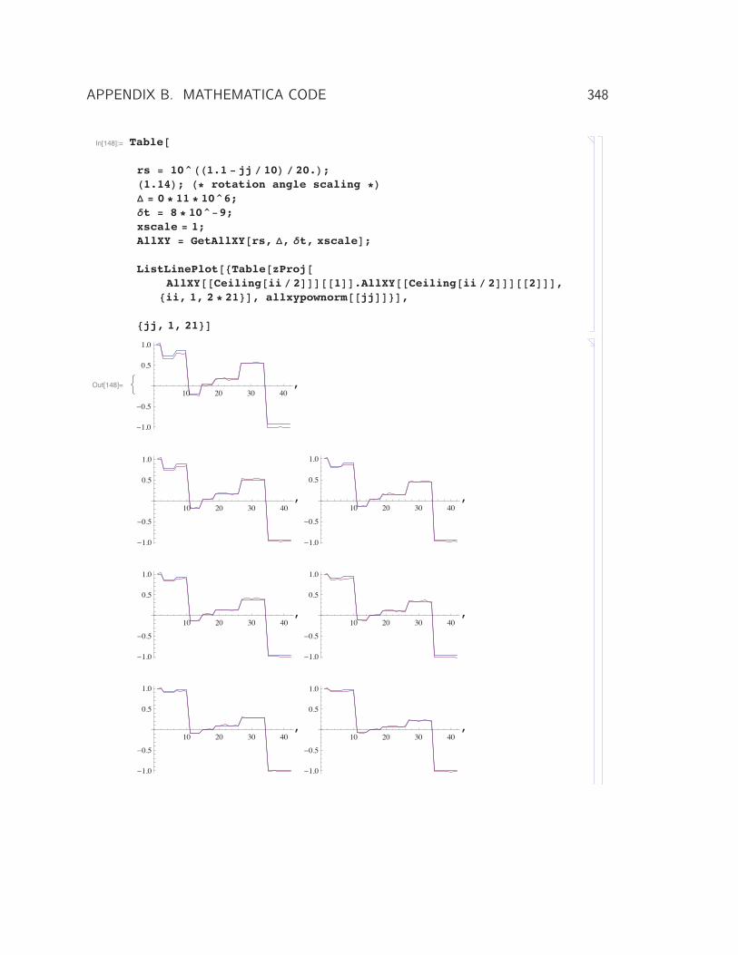
In[148]:= Table�
rs � 10^��1.1 � jj � 10� � 20.�;�1.14�; �� rotation angle scaling ��� � 0 � 11 � 10^6;Δt � 8 � 10^�9;xscale � 1;AllXY � GetAllXY�rs, �, Δt, xscale�;
ListLinePlot��Table�zProj�AllXY��Ceiling�ii � 2�����1��.AllXY��Ceiling�ii � 2�����2���,�ii, 1, 2 � 21��, allxypownorm��jj����,
�jj, 1, 21��
Out[148]= 10 20 30 40
�1.0
�0.5
0.5
1.0
,
10 20 30 40
�1.0
�0.5
0.5
1.0
,10 20 30 40
�1.0
�0.5
0.5
1.0
,
10 20 30 40
�1.0
�0.5
0.5
1.0
,10 20 30 40
�1.0
�0.5
0.5
1.0
,
10 20 30 40
�1.0
�0.5
0.5
1.0
,10 20 30 40
�1.0
�0.5
0.5
1.0
,
APPENDIX B. MATHEMATICA CODE 348

10 20 30 40
�1.0
�0.5
0.5
1.0
,10 20 30 40
�1.0
�0.5
0.5
1.0
,
10 20 30 40
�1.0
�0.5
0.5
1.0
,10 20 30 40
�1.0
�0.5
0.5
1.0
,
10 20 30 40
�1.0
�0.5
0.5
1.0
,10 20 30 40
�1.0
�0.5
0.5
1.0
,
10 20 30 40
�1.0
�0.5
0.5
1.0
,10 20 30 40
�1.0
�0.5
0.5
1.0
,
10 20 30 40
�1.0
�0.5
0.5
1.0
,10 20 30 40
�1.0
�0.5
0.5
1.0
,
10 20 30 40
�1.0
�0.5
0.5
1.0
,10 20 30 40
�1.0
�0.5
0.5
1.0
,
APPENDIX B. MATHEMATICA CODE 349
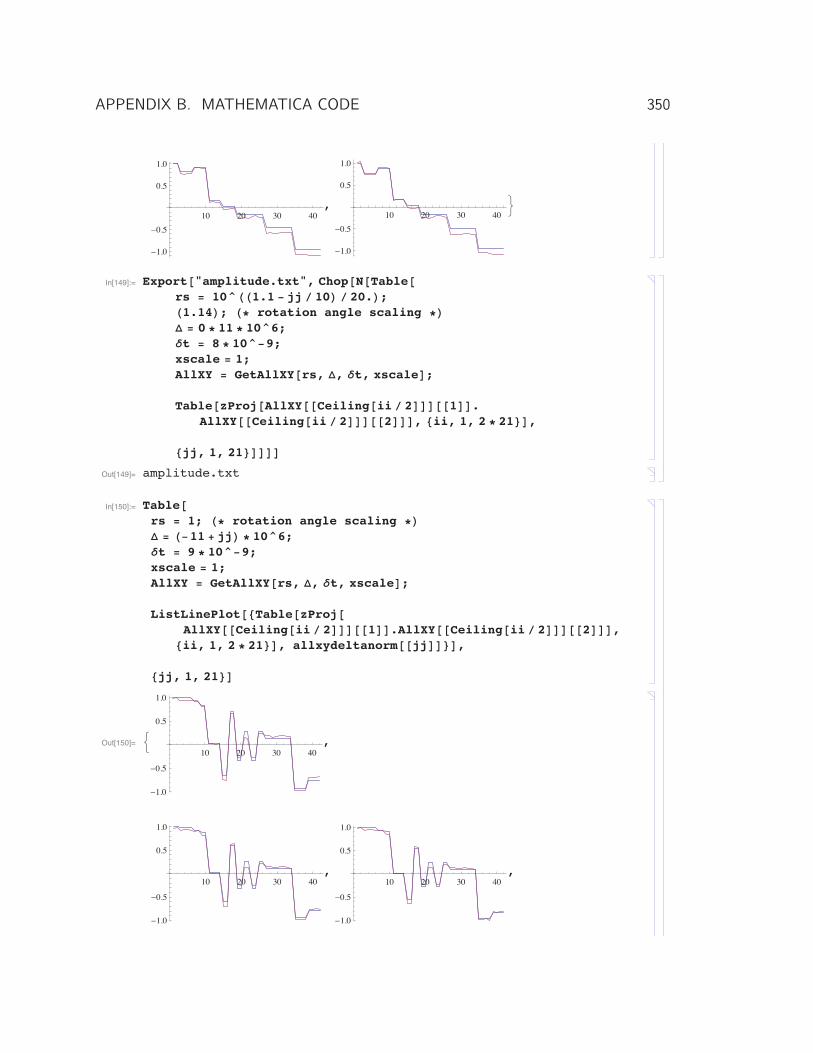
10 20 30 40
�1.0
�0.5
0.5
1.0
,10 20 30 40
�1.0
�0.5
0.5
1.0
�
In[149]:= Export�"amplitude.txt", Chop�N�Table�rs � 10^��1.1 � jj � 10� � 20.�;�1.14�; �� rotation angle scaling ��� � 0 � 11 � 10^6;Δt � 8 � 10^�9;xscale � 1;AllXY � GetAllXY�rs, �, Δt, xscale�;
Table�zProj�AllXY��Ceiling�ii � 2�����1��.AllXY��Ceiling�ii � 2�����2���, �ii, 1, 2 � 21��,
�jj, 1, 21�����Out[149]= amplitude.txt
In[150]:= Table�rs � 1; �� rotation angle scaling ��� � ��11 � jj� � 10^6;Δt � 9 � 10^�9;xscale � 1;AllXY � GetAllXY�rs, �, Δt, xscale�;
ListLinePlot��Table�zProj�AllXY��Ceiling�ii � 2�����1��.AllXY��Ceiling�ii � 2�����2���,�ii, 1, 2 � 21��, allxydeltanorm��jj����,
�jj, 1, 21��
Out[150]= 10 20 30 40
�1.0
�0.5
0.5
1.0
,
10 20 30 40
�1.0
�0.5
0.5
1.0
,10 20 30 40
�1.0
�0.5
0.5
1.0
,
APPENDIX B. MATHEMATICA CODE 350
10 20 30 40
�1.0
�0.5
0.5
1.0
,10 20 30 40
�1.0
�0.5
0.5
1.0
,
10 20 30 40
�1.0
�0.5
0.5
1.0
,10 20 30 40
�1.0
�0.5
0.5
1.0
,
10 20 30 40
�1.0
�0.5
0.5
1.0
,10 20 30 40
�1.0
�0.5
0.5
1.0
,
10 20 30 40
�1.0
�0.5
0.5
1.0
,10 20 30 40
�1.0
�0.5
0.5
1.0
,
10 20 30 40
�1.0
�0.5
0.5
1.0
,10 20 30 40
�1.0
�0.5
0.5
1.0
,
10 20 30 40
�1.0
�0.5
0.5
1.0
,10 20 30 40
�1.0
�0.5
0.5
1.0
,
APPENDIX B. MATHEMATICA CODE 351

10 20 30 40
�1.0
�0.5
0.5
1.0
,10 20 30 40
�1.0
�0.5
0.5
1.0
,
10 20 30 40
�1.0
�0.5
0.5
1.0
,10 20 30 40
�1.0
�0.5
0.5
1.0
,
10 20 30 40
�0.5
0.5
1.0
,10 20 30 40
�0.5
0.5
1.0
�
In[151]:= Export�"detuning.txt", Chop�N�Table�rs � 1; �� rotation angle scaling ��� � ��11 � jj� � 10^6;Δt � 9 � 10^�9;xscale � 1;AllXY � GetAllXY�rs, �, Δt, xscale�;
Table�zProj�AllXY��Ceiling�ii � 2�����1��.AllXY��Ceiling�ii � 2�����2���, �ii, 1, 2 � 21��,
�jj, 1, 21�����Out[151]= detuning.txt
In[153]:= Export�"xscale.txt",Chop�N�Table�rs � 1; �� rotation angle scaling ��� � 0 � 11 � 10^6;Δt � 8 � 10^�9;xscale � �0.96 � jj � 100� � 1.02 ;AllXY � GetAllXY�rs, �, Δt, xscale�;
Table�zProj�AllXY��Ceiling�ii � 2�����1��.AllXY��Ceiling�ii � 2�����2���, �ii, 1, 2 � 21��,
�jj, 0, 11�����Out[153]= xscale.txt
APPENDIX B. MATHEMATICA CODE 352
Copyright Permissions
• Figures 4.2, 4.12, 7.1, 7.4, 7.6, 7.10, 7.13, 7.15, 7.16, and 7.17 reproduced oradapted with permission from:L. DiCarlo, M. D. Reed, L. Sun, B. R. Johnson, J. M. Chow, J. M. Gambetta,L. Frunzio, S. M. Girvin, M. H. Devoret, and R. J. Schoelkopf, Nature 467,574–578 (2010).Copyright © 2010, Nature Publishing Group.
• Figures 6.3, 6.4, 6.5, and 6.7 reproduced with permission from:M. D. Reed, B. R. Johnson, A. A. Houck, L. DiCarlo, J. M. Chow, D. I. Schuster,L. Frunzio, and R. J. Schoelkopf, Appl. Phys. Lett. 96, 203110 (2010).Copyright © 2010, American Institute of Physics.
• Figures 6.8, 6.9, 6.10, 6.11, 6.12, 6.13, and 6.14 adapted with permission from:M. D. Reed, L. DiCarlo, B. R. Johnson, L. Sun, D. I. Schuster, L. Frunzio, and R. J.Schoelkopf, Phys. Rev. Lett. 105, 173601 (2010).Copyright © 2010, the American Physical Society.
• Figure 5.3 adapted with permission from:Hanhee Paik, D. I. Schuster, Lev S. Bishop, G. Kirchmair, G. Catelani, A. P. Sears,B. R. Johnson, M. J. Reagor, L. Frunzio, L. I. Glazman, S. M. Girvin, M. H.Devoret, and R. J. Schoelkopf, Phys. Rev. Lett. 107, 240501 (2011).Copyright © 2011, the American Physical Society.
• Figures 8.2, 8.5, 8.6, 8.8, 8.9, 8.10, 8.11, 8.12, 8.13, 8.14, 8.15, and 8.16reproduced or adapted with permission from:M. D. Reed, L. DiCarlo, S. E. Nigg, L. Sun, L. Frunzio, S. M. Girvin, and R. J.Schoelkopf, Nature 482, 382–385 (2012).Copyright © 2012, Nature Publishing Group.
353
