HEAD MOTION EVALUATION AND CORRECTION IN MAGNETOENCEPHALOGRAPHY

BY

INNA V. MCGOWIN

A Dissertation Submitted to the Graduate Faculty of

WAKE FOREST UNIVERSITY GRADUATE SCHOOL OF ARTS AND SCIENCES

in Partial Fulfillment of the Requirements

for the Degree of

DOCTOR OF PHILOSOPHY

Physics

May 2015

Winston-Salem, North Carolina

Approved By:

J. Daniel Bourland, Ph.D., Advisor

Dwayne W. Godwin, Ph.D., Chair

Daniel B. Kim-Shapiro, Ph.D.

V. Paúl Pauca, Ph.D.

Richard T. Williams, Ph.D.

ii

ACKNOWLEDGEMENTS

First and foremost, I thank my advisor, Dr. J. Daniel Bourland for his constant support,

encouragement, and advice throughout my graduate studies. I also would like to express

my gratitude for all the help, support and feedback I received from Dr. Dwayne W.

Godwin and his laboratory for neuroscience studies. Special thanks are given to Justin

B. Rawley and Greg E. Alberto for participating in the data collection and data analysis

discussions.

Also I would like to acknowledge and thank Dr. V. Paúl Pauca for his insights and

suggestions on my project from computer science perspectives.

I gratefully acknowledge the contribution of the Magnetoencephalography laboratory,

Wake Forest Baptist Medical Center, for making the data collection possible.

I would like to thank Bob Morris, Wake Forest University Department of Physics, for

helping designing and manufacturing the 3D Motion Platform used in the study.

Last but not least, I would like to thank all the members of the CTF Systems Inc. (A

Subsidiary of VSM MedTech Ltd., 15-1750 McLean Ave., Port Coquitlam, B.C)

especially Slobodan Mitrovic and Brent Taylor, for their help and contribution to my

knowledge of the MEG scanner operation and maintenance, and for providing the

software module for the SSS head motion correction method used in this project.

iii

TABLE OF CONTENTS

LIST OF TABLES ........................................................................................................... vi

LIST OF FIGURES ........................................................................................................ vii

LIST OF ABBREVIATIONS ............................................................................................ ix

ABSTRACT .................................................................................................................... xi

I. INTRODUCTION ......................................................................................................... 1

I.A Magnetoencephalography ..................................................................................... 1

a) Biomagnetic signal measurement ........................................................................ 2

b) Room shielding and Superconducting Quantum Interference Device .................. 3

I.B Introduction to neural activity of the brain ............................................................... 5

a) Action potential vs. postsynaptic potential ........................................................... 7

b) Primary current vs. volume current ...................................................................... 8

I.C Interpretation of MEG measurements .................................................................... 9

a) The inverse problem ...........................................................................................11

b) Beamformer analysis ..........................................................................................12

I.D The head motion problem .....................................................................................13

a) Head localization ................................................................................................14

b) Head motion compensation in prior art ...............................................................17

c) Head motion evaluation in healthy subjects ........................................................17

I.E Head motion correction methods ..........................................................................23

iv

a) Signal Space Separation ....................................................................................25

b) General Linear Modeling ....................................................................................33

II. METHODS AND MATERIALS ...................................................................................37

II.A 3D motion platform construction and application ..................................................37

a) Current Dipole Phantom .....................................................................................37

b) Data collection with motion .................................................................................41

II.B Motion correction performance and comparison ..................................................44

II.C Motion assessment criteria ..................................................................................44

1) Percent-Root-Difference .....................................................................................44

2) Pearson Product-Moment Correlation Coefficient ...............................................45

3) Signal-to-Noise Ratio .........................................................................................46

4) Localization accuracy .........................................................................................47

5) Signal coherence................................................................................................49

6) Average coherence calculation ...........................................................................51

III. RESULTS .................................................................................................................54

III.A Signal Space Separation vs. General Linear Modeling .......................................54

III.B Motion correction method of choice and its limitations ........................................69

III.C Theoretical approach to improve Signal Space Separation method ....................70

a) Sensor array shape and its fit approximation ......................................................71

b) Transformation from Cartesian to spheroidal coordinate system ........................77

c) Spheroidal harmonics expansion ........................................................................79

v

d) Forward and inverse transformation between spherical and spheroidal

coefficients .............................................................................................................82

IV. DISCUSSION ...........................................................................................................89

V. CONCLUSION ..........................................................................................................96

VI. REFERENCES.........................................................................................................98

VII. APPENDIX I .......................................................................................................... 103

VIII. CURRICULUM VITAE .......................................................................................... 105

vi

LIST OF TABLES

Table 1: Direction and extent of the Current Dipole phantom motion .............................43

Table 2: SSS vs. GLM motion correction methods comparison .....................................55

Table 3: Change in signal coherence and its fraction for SSS, GLM and SSSsm

correction methods for the filtered and unfiltered data sets ............................................65

Table 4: Numerical results for spherical, spheroidal and ellipsoidal surface approximation

for phantom and subject recordings ...............................................................................75

vii

LIST OF FIGURES

Figure 1: (a) CTF MEG™ scanner, (b) head positioning with fiducial coils (black wires),

(c) CTF MEG coordinate system (used with permission and courtesy of MEG

International Services Ltd) .............................................................................................. 2

Figure 2: Cerebral fissure, MEG sensor and Equivalent Current Dipole schematic ......... 7

Figure 3: MEG measurements (top left), contour maps (bottom left), and head model

(top right) and MEG-MRI co-registration (bottom right) ..................................................10

Figure 4: MEG sensor array in relation to head positioning ............................................14

Figure 5: Fiducial Localization Coils (used with permission of MEG International Services

Ltd) ................................................................................................................................15

Figure 6: CTF MEG Coordinate System (used with permission of MEG International

Services Ltd.) ................................................................................................................16

Figure 7: Maximum head motion in three directions for each scan ................................19

Figure 8: Head motion averaged across all subjects as a function of time .....................20

Figure 9: Maximum head rotation in three directions for each scan ...............................21

Figure 10: Mean head rotation differences around each axis .........................................22

Figure 11: Schematic of MEG helmet, brain location and internal & external sources

locations (not to scale) ...................................................................................................28

Figure 12: MEG 3D Motion Platform ..............................................................................38

Figure 13: The Current Dipole Phantom with one dipole inserted into the phantom head

......................................................................................................................................40

Figure 14: Current Dipole Localization ...........................................................................49

Figure 15: Change in PRD; SSS vs. GLM comparison for the unfiltered data set ..........56

Figure 16: Change in PRD; SSS vs. GLM comparison for the filtered data set ..............57

Figure 17: Change in CC; SSS vs. GLM comparison for the unfiltered data set .............58

viii

Figure 18: Change in CC; SSS vs. GLM comparison for the filtered data set .................58

Figure 19: Change in SNR; SSS vs. GLM comparison for the unfiltered data set ..........59

Figure 20: Change in SNR; SSS vs. GLM comparison for the filtered data set ..............60

Figure 21: Localization difference between ideal data and data corrected for the motion

with SSS and GLM for unfiltered data set ......................................................................61

Figure 22: Localization difference between ideal data and data corrected for the motion

with SSS and GLM for filtered data set ..........................................................................62

Figure 23: Average Coherence Strength for all motions in the unfiltered data set ..........63

Figure 24: Average Coherence Fraction for all motions in the unfiltered data set ..........64

Figure 25: Average Coherence Strength for all motion in the filtered data set................66

Figure 26: Average Coherence Fraction for all motion in the filtered data set ................67

Figure 27: Ideal data segment vs. the SSS, GLM and SSSsm corrected data segments

for one channel recording at the maximum extent of the motion ....................................68

Figure 28: Subject and Phantom sensor arrays coordinates & orientation .....................73

Figure 29: Spherical, spheroidal and ellipsoidal surface fitting for Phantom and subject

recordings .....................................................................................................................74

Figure 30: Oblate (left column) and prolate (right column) spheroids and their coordinate

systems in X-Z plane for φ = 0 .......................................................................................78

Figure 31: MEG signal dimensionality with the Orthogonal Matching Pursuit method ....88

ix

LIST OF ABBREVIATIONS

µA Microampere

µT Microtesla

2D Two dimensional

Al Aluminum

AP Action Potential

BSCCO Bismuth strontium calcium copper oxide

CC Pearson Product-Moment Correlation Coefficient

cm Centimeter

Cu Copper

DC Direct Current

fMRI Functional Magnetic Resonance Imaging

fT Femtotesla

GLM General Linear Modeling

Hz Hertz

JJ Josephson Junction

K Kelvin

kHz Kilohertz

x

MEG Magnetoencephalography

mm Millimeter

MNE Minimum Norm Estimate

MRI Magnetic Resonance Imaging

ms Millisecond

OMP Orthogonal Matching Pursuit

PRD Percent Root Difference

PSP Postsynaptic Potential

RF Radio frequency

SNR Signal-to-Noise Ratio

SQUID Superconducting Quantum Interference Device

SSS Signal Space Separation

T Tesla

tSSS Spatiotemporal Signal Space Separation

V Volt

xi

ABSTRACT

McGowin, Inna V.

HEAD MOTION EVALUATION AND CORRECTION IN

MAGNETOENCEPHALOGRAPHY

Dissertation under the direction of

J. Daniel Bourland, Ph.D., Professor of Radiation Oncology,

Biomedical Engineering, and Physics (Adjunct)

Head motions during magnetoencephalography (MEG) data acquisition lead to

inaccuracy in MEG signal localization and statistical sensitivity. Multiple head motion

correction methods have been developed and validated to insure the head motion

effects are removed, with the aim of improving localization accuracy and statistical

sensitivity. This study investigated the amount and extent of the head motion during

MEG resting state recordings with 80 subjects and supported the previously known

downward motion of the head during scanning. Rotational motion was quite negligible

and had no preferred direction. These findings led to investigation of the effectiveness of

two motion correction methods, Single Space Separation (SSS) and General Linear

Modeling (GLM) for correction of translational motion. SSS and GLM were evaluated

and compared by five assessment criteria: Percent Root Difference (PRD), Pearson

Product-Moment Correlation Coefficient (CC), Signal-to-Noise Ratio (SNR), localization

accuracy and signal coherence. Quantitative comparison revealed that SSS is superior

for data accuracy, resemblance and localization precision when applied to the pre-

filtered recordings compared to GLM. The localization accuracy of SSS is within 1-3 mm

for all motion directions up to 2 cm. SSS reduces the coherence strength and the total

xii

number of the coherent links in the pre-filtered data. GLM improves/reduces data

accuracy and resemblance when applied to unfiltered/pre-filtered data respectively. The

localization precision of GLM reduces approximately linearly with the motion extent.

GLM improves localization accuracy in the unfiltered/pre-filtered recordings by a factor of

2-4. GLM does not change coherence strength and only slightly decreases/increased the

total number of the coherent links on the sensors’ level when applied to the

unfiltered/filtered data respectively. This study concluded that the SSS method yields

better localization accuracy and better data quality improvement than GLM when applied

to the pre-filtered MEG recordings. SSS was further investigated here and a route for its

improvement was suggested. This route uses oblate/prolate spheroidal harmonics in

place of the spherical harmonics expansion and preserves the simplicity of the

translation and rotation transformations of the spherical harmonic functions. The

preservation is achieved via forward and inverse spherical to spheroidal expansion

coefficients transformations allowing motion correction on spherical harmonics

coefficients.

1

I. INTRODUCTION

I.A Magnetoencephalography

Magnetoencephalography (MEG) is an imaging technique that measures the

neuromagnetic field and maps its sources produced by neuronal activities in the brain.

The technique allows recording of temporal and spatial magnetic signal changes from

outside of the brain space and mapping the signal sources into the brain space in non-

invasive way. Figure 1(a) depicts the MISL CTF MEG™ scanner used in this study and

Figure 1(b) shows typical head positing within the helmet and assigned coordinate

system shown in Figure 1(c). All images in Figure 1 are used with permission and

courtesy of MEG International Services Ltd.

Typically, measured MEG signals are co-registered with the subject’s structural

Magnetic Resonance Imaging (MRI) scan to allow individual head modeling and source

localization with reference to the subject’s anatomy. MEG is a direct measure of time-

variant electric currents within the brain, with a spatial resolution between a few

millimeters and a few centimeters and temporal resolution of a millisecond 1.

2

Figure 1: (a) CTF MEG™ scanner, (b) head positioning with fiducial coils (black wires),

(c) CTF MEG coordinate system (used with permission and courtesy of MEG

International Services Ltd)

a) Biomagnetic signal measurement

Neuromagnetic fields are very weak, on the order of 10-500 fT (1fT = 10-15 Tesla). In

comparison with the Earth magnetic field of 65 µT (1 µT = 10-6 Tesla) the neuromagnetic

fields are about 109 times weaker 2. To record such weak magnetic fields in a relatively

high magnetic noise environment, a magnetically shielded room and a highly sensitive

magnetic field detector are required.

3

b) Room shielding and Superconducting Quantum Interference Device

Magnetic shielding can be achieved via combinations of four different passive or active

methods: ferromagnetic, eddy-current, active compensation and high temperature

superconducting shielding 3. Ferromagnetic shielding is a passive method that uses

magnetic flux-entrapment by a ferromagnetic material of high permeability. Permeability

of a material is the degree to which the material can support a formation of the magnetic

field within itself, in other words, it is the degree of magnetization when the material is

exposed to the external magnetic field. The high permeability material used in MEG

shielding is called µ-metal (approximately 77% nickel, 16% iron, 5% copper and 2%

chromium or molybdenum). When a static or/and low-frequency magnetic field is

incident on such material the field prefers to travel inside the material via the path of

least magnetic reluctance (equivalent to an electric resistance for electric currents), thus

interrupting the field propagation to regions beyond and forming a shield. This method

redirects the Earth’s static magnetic field along the walls, ceiling and floor and blocks the

field from entering the MEG scanner room.

High-frequency magnetic perturbations, such as RF (radio frequency) signals, are

attenuated by highly conductive metals (Cu, Al) via eddy-current induction. Eddy

currents in a conductor are closed currents that generate magnetic fields via induction in

a direction that opposes any changes in the external magnetic flux, thus generating a

shielding effect. Ferromagnetic and eddy-current shielding is achieved by successive

layers of µ-metal, Cu and Al in the MEG room walls, ceiling and floor.

4

In an alternative method, high temperature superconducting shielding can be achieved

with a hollow cylinder made of the high temperature superconductor bismuth strontium

calcium copper oxide (BSCCO) with the critical temperatures of ~95 K, or 104 K, or 108

K with two more ferromagnetic cylinders attached to both ends of the superconducting

cylinder to enhance the shielding effect. The cylinder arrangement is large enough to

enclose a human body and MEG couch and provides an attenuation factor between 10-6

and 10-8. This shielding method is based on the property of the interaction between

supercurrent and magnetic flux: weak magnetic fields are expelled from a

superconductive volume. Currently, this shielding method is not employed with MEG

systems and was not available or used in this study 4.

Distant low frequency noise created by moving metal objects, such as cars, elevators

and others, is actively shielded by gradiometers in the sensing part of the MEG gantry. A

gradiometer is a set of magnetometers connected in axial or planar fashion. A

magnetometer is a device to measure magnetic field strength and/or its direction.

Two magnetometers separated by some distance (3-5 cm) and connected in series or

parallel such that the resultant currents oppose each other represent a gradiometer used

to actively shield a distant magnetic noise.

Because the changing magnetic field of a distance source (>> 5 cm away) is relatively

uniform across the gradiometer baseline, magnetometers produce the same currents of

opposite direction and their magnetic fields will cancel each other, thus successfully

cancelling the signal from the distant source. Magnetic signal from a near source, such

5

as a human head inside the MEG helmet, will produce a magnetic gradient across the 3-

5 cm distance that is not cancelled, thus producing non-zero output signal.

In MEG applications used in this study the gradiometer is a primary sensor that is

coupled inductively to a Superconducting Quantum Interference Device (SQUID) 2. A

SQUID is a very sensitive vector magnetometer used to detect and quantify small

changes in magnetic flux in a superconducting environment (superconductor Niobium

operates at 4.2 Kelvin in liquid helium). A DC SQUID is typically used in the MEG

scanner and is a superconducting ring interrupted by two Josephson junctions (JJ). The

JJ is a small insulating link between two sides of the superconductor. The principle of

SQUID operation will not be discussed in depth here and can be found elsewhere 5. In

short, the principle of SQUID operation is based on JJ quantum tunneling by a Cooper

pair (pair of two electrons in a superconducting state) and the flux quantization

phenomenon. It is a property of a supercurrent that the magnetic flux passing through

any area bounded by such current is quantized by the magnetic flux quantum Φ0=h/2e

(h is the Planck’s constant and e is the electron charge). A DC SQUID is operated under

a bias current that leads to voltage oscillation across JJs due to the external magnetic

flux passing through the superconducting loop. The voltage oscillates with the period Φ0

and constitutes the measured signal.

I.B Introduction to neural activity of the brain

The MEG signal is generated by ionic currents in neurons of the brain (intracellular

current) and their surrounding ionic environment (extracellular current). A pyramidal cell

is a neuron type with a pyramidal shaped cell body and two distinct dendritic trees

6

(apical and basal). Pyramidal neurons bodies and dendritic trees are found in the grey

matter of the brain including the cerebral cortex, hippocampus, and amygdala, and are

oriented perpendicularly to the cortical surface. Pyramidal cells are among the largest

neurons in the brain; their apical dendrites reach out almost parallel to each other, which

allows ionic signal summation to yield a net current vector. Pyramidal cells are organized

in macro-assemblies allowing spatial summation of signals from different cells. Also

when neurons in such assembles are activated almost simultaneously, the temporal

signal summation takes place. MEG signal detection depends on the neuronal ensemble

orientation in relation to the skull. It is believed a layer of pyramidal cells situated

tangentially to the skull is responsible for the MEG signal 2. A layer of the pyramidal cells

activated simultaneously can be modeled by an equivalent current dipole, a vector

quantity representing macroscopic direction, orientation and strength of the neuronal

activity within the brain 6. In Figure 2 a schematic drawing of the cortical fold represents

an area of the pyramidal column marked as cortex. Black arrows on the left side of the

figure show one of the two possible neuronal current directions with their orientation in

respect to a MEG sensor. The right side of Figure 2 shows a zoomed in image of the

tangential current dipole (a thick black arrow), its volume currents (thin black lines with

arrows showing the direction of the current flow) and the corresponding magnetic field

shown in blue with its direction and orientation. The magnetic field from tangential (to the

skull/scalp) sources is the most easily detectable by MEG sensors.

7

Figure 2: Cerebral fissure, MEG sensor and Equivalent Current Dipole schematic

a) Action potential vs. postsynaptic potential

The electrical activity of a neuron can be divided into postsynaptic potential (PSP) and

action potential (AP). The postsynaptic potential is due to the change in the membrane

permeability of the postsynaptic cell body or dendrites which leads to ionic current along

the interior and exterior of the cell body membrane. PSP is mediated by

neurotransmitters, but also may have contributions from active membrane properties,

such as voltage-gated ion channels 2, 7.

The PSP current from a distance r acts like a current dipole and its magnetic field

strength falls off as 1/r2. Change in the cell membrane potential depends on the amount

and type of neurotransmitters released and the PSP voltage has no fixed amplitude.

Produced currents are short-lived (∼ 1 ms). Each neuron receives a signal from many

other neurons (thousands of inputs). These inputs undergo spatial and temporal

summation leading to stronger and longer current pulses 3.

8

Action potential (AP) is a propagation of electric current along the cell’s axon due to the

threshold voltage reached at the axon hillock; it lasts 1-2 ms and has fixed amplitude 3.

AP ionic current can be represented by two dipoles of opposite directions called a

quadruple. Quadruple magnetic field strength falls off with the distance r as 1/r3.

Due to spatial and temporal summation PSP current lasts longer than AP current.

Additionally, the magnetic field created by the PSP signal decreases slower with

distance than that from the AP signal thus the majority of the MEG signal detected is

likely from the PSP currents. One neuron does not produce a detectable MEG signal.

Many temporarily synchronized neurons are needed (104 – 105 cells) 2.

b) Primary current vs. volume current

As established above, the PSP contributes to the measured magnetic signal. From the

biological perspective, there should be no charge accumulation due to neuronal

activities, thus currents flowing in or out of the membrane are compensated by

extracellular currents of opposite directions 3. The current due to PSP can be further

divided into primary current �� (intracellular current) and volume current �� (extracellular

current) such that the total current �� will lead to charge conservation:

�� = �� + �� = �� − � Equation ( 1 )

In Equation ( 1 ) is the conductivity of the brain (assumed to be homogeneous) and �

is the electric potential created by the primary current. Division into primary and volume

9

currents is important for MEG signal detection and localization, as it is the primary

current that is detected and localized as the direct measurement of the neuronal activity.

Under some special geometry configurations for the conductive volume such as an

infinite conductor, semi-infinite slab or spherical volume, only primary currents contribute

to the magnetic signal measured outside of the conductor. It is customary to use a

homogeneous spherical volume conductor to model a human brain for MEG signal

localization methods. In reality, neither the human head is perfectly spherical nor does

the MEG sensor shape follows a spherical surface which leads to signal contamination

by the volume currents. MEG is mainly sensitive to tangential source orientation in

relation to the skull surface for superficial locations, such as would be found for

pyramidal cells aligned to sulci oriented normally to the skull surface, but non-tangential

sources can contribute up to 20% of the measured signal 8.

I.C Interpretation of MEG measurements

MEG data represent a set of measurements of the total magnetic field produced by brain

activity and measured around the head as a function of time. The challenge in

processing and interpreting MEG signals is to determine the exact locations, orientations

and amplitudes of the individual sources (generators) within the brain from the externally

measured signal (Figure 3). Such a problem is called an inverse problem, whereby

external data are projected internally to calculated potential origins.

In Figure 3 the top left corner shows an overlap of all MEG channels measurements

(275 waveforms) with an evoked primary response peak in fT (the butterfly peak

selected by dashed lines) plotted as a function of time in sec. The bottom left corner of

10

Figure 3 displays nine contour maps of the nine evenly spread time responses on both

sides of 105 ms time sample. The contour maps are created by projecting the measured

MEG signal on to a circle; the maps are used in MEG signal analysis as a quick visual

reference to estimate a possible time location of an evoked response. The top right

corner of Figure 3 shows the geometrical relation between MEG channels (blue hollow

circles), a human brain (reconstructed from MRI, displayed below) and the MEG

coordinate system defined by the locations of the fiducial coils shown in red.

Figure 3: MEG measurements (top left), contour maps (bottom left), and head model

(top right) and MEG-MRI co-registration (bottom right)

11

It was shown by H. Helmholtz in 1853 that electromagnetic inverse problems do not

have unique solutions: a current distribution inside a conductor cannot be retrieved

uniquely from the outside electromagnetic field because some currents inside the

conductor can be electrically or magnetically silent outside of the conductor 9. Such silent

sources can be added to the solution without affecting the field outside. An example of a

magnetically silent source is a radial current (current directed along the radius) in a

spherical conductor. A current loop inside a conductor is an example of the electrically

silent source: such source produces a measureable magnetic field outside the conductor

but no measureable electric field 2. Thus additional constraints and assumptions must be

introduced into the problem to enable determination of the best possible solution among

many.

a) The inverse problem

To solve the inverse problem a forward solution is determined based on a given head

model (spherical or more realistic head shape), quasi-static approximation of Maxwell’s

equations and MEG measurements 2. In the simplest case, such as a spherical head

model and one active dipolar source, the Biot-Savart law can be used to calculate the

magnetic field outside the head:

� �� = ��� � � � ��� × � − ���|� − ��|�� ��� = ��� � �∆� � − ���|� − ��|�� Equation ( 2 )

In Equation ( 2 )

�� is the magnetic permeability of the free space used here because the brain tissue can

12

be approximated with water,

� ��� is the current density distribution at the location ��inside the head,

�∆� is the current dipole moment of the length ∆� and current �,

� is the location of the measurement (MEG sensor location) outside of the conductive

volume.

As it can be seen from this simplest case, the geometrical relation between the source

location and the measurement location defines the strength and direction of the

magnetic field measured.

b) Beamformer analysis

Another MEG signal interpretation approach is “beamforming”. Beamforming is a digital

spatial filtering technique borrowed from the radar field. The technique is based on the

spatial suppression or enhancement idea in sensor array measurements for directional

signal transmission or reception of electromagnetic or sound waves. This is achieved by

combining sensor signals such that a desirable interference pattern is obtained,

destructive or constructive. The beamforming determines a set of weights for each voxel

within the brain that allows the signal power to be extracted for that voxel while

suppressing a majority of the signal from outside the voxel 10.

Calculation of these weights involves determination of the leadfield matrix L, also called

the gain matrix. The leadfield matrix consists of a set of coefficients that tells how a

current in a given voxel produces a signal measured by a given sensor. The leadfield

values are calculated for each voxel-sensor pair and based on the exactly known

13

geometric location of each sensor and each voxel. This calculation is computationally

expensive and performed once for each MEG data assuming that the subject’s head

position remains fixed throughout the recording.

I.D The head motion problem

The MISL CTF MEG™ head helmet (formerly VMS CTF, now, MEG International

Services Ltd, Coquitlam, BC, CA) for magnetoencephalography (MEG) imaging is

designed to accommodate most head sizes and provides the best fit for a larger adult

head, about 60 cm in circumference (Figure 4). Prior to MEG acquisition a subject’s

head is positioned within the helmet without any rigid fixation (Figure 1b). As a result, the

helmet permits head motion during and between scan sessions for those with smaller

head sizes or changing posture. Head movements during the scan reduce localization

accuracy (in the inverse problem or beamforming) and statistical sensitivity of the

analysis, requiring head motion monitoring and correction (or rejection) of the recorded

MEG data 11, 12. The head movements are more pronounced in younger or less

cooperative subjects but also can be a problem during prolong recordings or

experimental recordings requiring a subject to perform a task while in the scanner.

14

Figure 4: MEG sensor array in relation to head positioning

a) Head localization

In order to relate recorded MEG data to current sources within the brain, head position

relative to the helmet (and thus to the sensor array) must be known. This is

accomplished by use of three or four fiducial coils attached to pre-defined head

landmarks: left and right pre-auricular points, and a nasion point. Also, an inion point can

be used in case of four fiducial marks (Figure 1b).The fiducial coils are small current

loops representing magnetic dipoles (Figure 5). The coils are energized by sinusoidal

currents of unique frequencies outside of the frequency range in interest (brain signals)

and are not power-line frequencies (e.g. 60 Hz) or its harmonics 13.

15

Figure 5: Fiducial Localization Coils (used with permission of MEG International Services

Ltd)

The fiducial coils’ signals are recorded continuously and concurrently with the brain

signal, and then filtered out and localized with the Magnetic Dipole Fitting method to

determine the head coordinate system in relation to the sensor array.

The origin of the head coordinate system for the MISL CTF MEG™ system is defined as

the middle point between left and right pre-auricular coil locations. The positive X axis is

a line passing from the origin to the nasion coil location. The Y axis is set perpendicularly

16

to the X axis through the origin and may or may not coincide with the right-left pre-

auricular line. The Y axis is positive in the direction from the origin to the left pre-

auricular point. The Z axis is perpendicular to X-Y plane and its positive direction is in

accordance with the right-handed coordinate system rule (Figure 6). In Figure 6 location

of the right pre-auricular point is marked with red, of the left with green and the nasion

point is in purple.

Figure 6: CTF MEG Coordinate System (used with permission of MEG International

Services Ltd.)

17

Because the reference fiducial coils’ signals can be recorded continuously, it is possible

to monitor head position throughout the recording. Head movements are calculated as

the difference between the current head position and the initial head position, the

position of the head at the beginning of the recording.

b) Head motion compensation in prior art

The head motion problem is a well-known and recognized among the MEG community.

For instance, head movements in 19 children (age 8-12) during a cognitive task were

studied by Wehner et al., 2008, and showed average motion of 3-26 mm with the largest

motion in the up-down direction 14. There have been no head movement studies

performed on a larger group of subjects and/or in the context of the resting state MEG

recordings. The resting state recording is usually performed with a subject in the upright

sitting position with eyes opened. The subject is asked to gaze at the same point and

remain still for 8-10 min.

c) Head motion evaluation in healthy subjects

As a part of preliminary work to investigate head motion for its magnitude and preferred

directions, 144 MEG scans were analyzed retrospectively for a large group of 80 healthy

volunteers. This preliminary work established motion parameters and their ranges for the

study of the head motion correction methods. Under an Institutional Review Board-

approved Head Trauma Study (IRB # 00014350) 15, more than 144 MEG resting state

scans (8 min each) were collected with 80 healthy volunteers on MISL CTF MEG™

275-sensor MEG scanner. These MEG data were analyzed retrospectively for head

motion to determine the range and magnitude of motion, before quantitative assessment

18

of motion correction methods. The subjects were males, players of youth (middle school)

or high school football teams; age range is 10-18 years. All resting state scans were

collected in the upright sitting position with eyes opened. Only the best 144 data sets

with minimal head motion were retained for future network analysis thus providing limited

data to study head motion in the scanner. In spite of this limitation, it was possible to

detect the direction of the most frequent and preferred head motion, which was in the

downward direction, an effect of slouching during the scan due to relaxation and/or

fatigue. The trend can be seen in the analysis of the maximum head motion for each

subject: the maximum motion along Z axis is statistically different from the maximum

motions along X or Y axes with p-value << 0.05 calculated in Matlab R2010b with the

Welch's t test (Figure 7). The test result showed that the mean maximum head deviation

along Z axis is the largest amongst these three directions. There is no statistical

difference between motions along X and Y axes with p > 0.05. The Welch's t test was

chosen as a statistical measure in this study because it tests the hypothesis that the

mean of two independent populations with unequal variances is the same or that the

mean of one population is statistically larger than of the other.

The maximum head motion was calculated from measured (with three fiducial coils)

head positions for three second intervals in two steps:

1) Find the difference between the current head position and the initial head position for

each 3 sec interval;

2) Search for maximum X, Y and Z values in the resultant data for each subject.

With exception of about 20 scans, the translational motion along the Z axis was

preferred and maximal compared to all other directions (Figure 7).

19

Figure 7: Maximum head motion in three directions for each scan

The same trend is supported by averaged head motion for all subjects as a function of

time: all directions are statistically different with p-values << 0.05 (Welch's t test) with the

major finding of a gradual and systematic head movement in the downward Z direction

(Figure 8). The averaged head motion was calculated across all subjects’ head motion

data in three seconds intervals along each axis.

20

Figure 8: Head motion averaged across all subjects as a function of time

The downward direction agrees with the direction detected by Wehner et al., 2008 14.

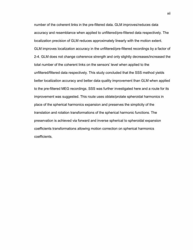
The maximum head rotation was calculated similarly to the maximum head motion.

Maximum head rotation did not exceed 1.50 and was on average 0.50 for a majority of

the subjects with no preferred direction of rotation, p-value > 0.05 (Figure 9). Analysis of

the head rotation averaged across 144 scans revealed no dependency or preferred

direction. Average degree of rotation across all subjects did not exceed 0.050 and did not

support the expectation of the preferred direction: positive rotation around X axis (chin

down rotation) (Figure 10). Differences in average head rotation around all axes test with

a p-value << 0.05 with exception for rotation around X axis vs. Z axis with a p-value of

0.07 (Welch's t test).

21

Figure 9: Maximum head rotation in three directions for each scan

22

Figure 10: Mean head rotation differences around each axis

Thus the translational head motion is more notable than the rotational with a preferred

downward directional movement along the Z axis. Head motion would be even more

pronounced for the recordings of any evoked response fields, i.e. recordings of

biomagnetic fields while the subject is performing a prompted task in the scanner 14.

This head motion study with 80 healthy volunteers showed that head motion is

essentially only translational, enabling study of the effects of head motion correction

algorithms in relation to the translational motion alone. Examination of the translational

motion along all axes and its correction was performed using a MEG compatible 3D

motion platform (built in-house) combined with the Current Dipole phantom provided with

the MEG system, as described in the Methods and Materials section.

23

I.E Head motion correction methods

All MEG source localization methods assume that the head position is fixed in relation to

the sensor array throughout the recording and all calculations are done in relation to the

initial head position measured in the head localization step prior to the MEG data

collection. In reality, as it was shown in the I.D (c) section, some head motion exists

mostly in the downward direction. Currently in the clinical and research settings MEG

recording with head motion of 5 mm or less is accepted for the analysis as if no head

motion happened. The 5 mm limit is based on empirical knowledge of an average head

motion among the patients and sets a limit on clinical localization accuracy.

The absence of head motion is important because the measured magnetic field

distribution around the head depends on the sensor array surface (planar, spherical or

head-shaped) and its geometrical orientation in space in relation to the source signal. In

other words, it depends on the X, Y, and Z components of the magnetic field vector � ��

measured at point �:

� ����������� = �!!" + �##" + �$$% Equation ( 3 )

The head motion problem can be dealt with by two general approaches:

1) Avoid head motion all together.

2) Remove or compensate head motion in the data offline.

In approach (1) Avoid head motion all together, motion can be minimized by

a) instructing each subject to remain still, to memorize their head position in the helmet,

and to attempt to return to that position every time the head motion happens;

b) using an online head repositioning system allowing head position visualization during

24

the recording by both the operator and the subject 12;

c) using MEG-compatible tools for rigid fixation of the head such as an inflatable

headband, bite-block, or silicon head-cast; these tools are prohibited to use for patients

with epilepsies or some other neurological disorders.

In the second approach (Remove or compensate head motion offline) as an additional

data processing step, there are two general categories:

a) Head motion compensation at the source level: the head motion is taken into account

when brain sources are localized via construction of the leadfield matrix and its inverse.

The leadfield matrix is assumed to be independent of time if no head motion happens.

When motion is introduced the leadfield matrix can be calculated:

- for each trial or time-window first and then averaged across all trials (or time-windows);

- or, for an average head position first calculated for all trials (or time-windows) and then

a blurred (but only one) leadfield matrix is determined and its inverse is applied to the

average data to localize the brain sources 12.

Both the Minimum Norm Estimate (MNE) and General Linear Modeling (GLM) head

motion correction are source level methods 12, 16.

b) Head motion compensation at the sensor level involves signal interpolation,

extrapolation and realignment such that the resultant signal will contain measurements

that would be recorded without the head motion. Ideally, this compensated signal should

be suitable for any further signal processing steps such as signal intensity and shape

analysis or source localization and statistical analysis. Signal Space Separation (SSS)

and General Linear Modeling (GLM) motion correction are examples of sensor level

methods 12, 17.

25

Because the SSS method is commercially implemented with Elekta Neuromag®

TRIUX™ and GLM method is easily available as a free Matlab toolbox in FieldTrip, these

two methods were chosen in this study for quantitative evaluation, comparison and

further improvement under the conditions of most popular head motion correction

methods in MEG community 12, 18, 19. These two methods are now reviewed.

a) Signal Space Separation

The SSS method is based on a quasi-static approximation of Maxwell’s equations using

a solid spherical harmonics expansion. SSS separates the signals coming from the

inside and outside of the MEG helmet, rejects the outside signals and corrects the inside

signals for the head motion. The SSS expansion is related to the head coordinate

system (determined by three fiducial coils on the subject’s head) and creates a device-

independent representation of the MEG data.

Because MEG sensor array consists of discrete number of sensors (MISL CTF MEG

array has 275-primary and 19-reference sensors) distributed over the top part of the

head, the MEG measurements are discrete and it is reasonable to discretize the

magnetic field these measurements represent. Discretization is done by a truncated

expansion of the magnetic field as a linear combination of certain basis functions, e.g.

spherical harmonics. Because the degree of freedom of any measured MEG brain signal

is less than 200 and the number of MEG sensors is more than 200 any measured MEG

signal can be uniquely decomposed into a device-independent representation 20.

26

Physiological frequencies of brain electrical signals are in the range of 0.1 Hz to 1 kHz 2.

This range allows the use of the quasi-static approximation of Maxwell’s equations:

∙ ' = ()� Equation ( 4 )

× ' = *�*� Equation ( 5 )

∙ � = � Equation ( 6 ) × � = �� +� + )�*'*� ,

Equation ( 7 )

The approximation neglects effects of the time-varying magnetic and electric fields, i.e.

terms *�/*� and *'/*� are negligibly small compared to the cellular currents and can

be set to zero. The measurements of the magnetic field � are collected in the source-

free region of the sensors array, thus Equation ( 7 ) becomes × � = � and now

magnetic field � can be represented with its magnetic scalar potential:

� = −��. Equation ( 8 )

In Equation ( 8 ) Ψ is the magnetic scalar potential used to calculate magnetic field.

Combining the simplified Equation ( 7 ) with Equation ( 8 ) yields the Laplace’s equation

(Equation ( 9 )) 2.

/. = � Equation ( 9 )

27

A general solution to the Laplace’s equation is given by Equation ( 10 ):

. �� = 0�� � � ��|1 − �| �� Equation ( 10 )

In Equation ( 10 )

1 is the sensor location (point of measurement),

� is the source location which can be both inside and outside of the helmet such that

1 > �34� or 1 < �6!� respectively,

� �� is the current density distribution.

Figure 11 shows schematic drawing of the MEG helmet with its sensor volume (a blue

spherical shell) within which one sensor is displayed (dark blue oval), the brain volume,

and three vectors 1, �34� and �6!� used in Equation ( 7 ).

28

Figure 11: Schematic of MEG helmet, brain location and internal & external sources

locations (not to scale)

The discrete solution Ψ can be obtained via spherical harmonics expansion of the

inverse distance 1 |1 − �|9 21:

. �� = 0�� : : ;<�=�>�>01� + ?�=��1>�>0@A�= B, C��=D>�

E�D0

Equation ( 11 )

29

In Equation ( 11 )

A�= B, C� are spherical harmonic functions of degree � and order =,

� and = are integers such that � ≥ 0 and – � ≤ = ≤ � . The use of the spherical harmonics expansion assumes that the data were collected

over a spherical surface of radius 1. Thus 1 = IJ4K� and Equation ( 11 ) can be

reduced to Equation ( 12 ) by inclusion of these constants within the spherical harmonics

coefficients:

. �� = 0�� : : ;<�=�>�>0 + ?�=��@A�= B, C��=D>�

E�D�

Equation ( 12 )

The first term in the summation <�=�>�>0 represents the internal sources (sources within

the helmet) and the second term ?�=�� represents the external sources thus allowing for

signal separation into internal and external components as shown in Equation ( 13 ):

. �� = . ��34�6�4<� + . ��6!�6�4<� Equation ( 13 )

In Equation ( 12 ) <�= and ?�= are scalar expansion coefficients called multipole

moments. The moments are related to the current distribution inside and outside of the

helmet. The separation into internal and external signals is possible because the sensor

array is located in the source-free volume and divides the total space into two separate

subspaces.

30

Inserting Equation ( 12 ) into Equation ( 8 ) gives Equation ( 14 ) allowing the measured

magnetic field � �� to be expressed in terms of vector spherical harmonic functions

L�= B, C� and M�= B, C� 20:

� �� = − ���� : : N<�=�>�>/L�= B, C� + ?�=��>0M�= B, C�O�=D>�

E�D�

Equation ( 14 )

The key point in Equation ( 14 ) is that the vector spherical harmonic expansion of the

magnetic field � �� has the same multipole moments, <�= and ?�=, as the expansion

for the magnetic scalar potential . �� in Equation ( 12 ).

To obtain the spherical harmonics expansion the multipole moments must be

determined such that they properly represent the measured magnetic field � �� on the

sensors. The MEG sensor array covers only approximately 60% of the sphere. The

expansion should not lead to creation of large magnetic fields in the areas not covered

by the array 13, 22.

The SSS method is based on the application of the spherical harmonics expansion to all

channel recordings and is discussed in depth elsewhere 13, 17, 22. The SSS method used

in this study is the software module implemented by MISL CTF MEG™ for research

purposes only and from here and on will be referred to as the SSS correction.

31

Decomposition of the measured MEG signal into the spherical harmonics representation

is device independent as it is related to the head coordinate system only. This allows

transferring the decomposed signal between different sensor array positions in a head

motion correction algorithm. The head translation and rotation can be found from the

continuous head localization data, these data can be converted into rotation and

translation operators for spherical harmonics and applied to the spherical harmonics

coefficients (the multipole moments).

Head motion can be understood as translation and rotation of the initial coordinate

system (x y z) to the final (x’ y’ z’). The center of each coordinate system is known from

the continuous head localization data. One way to transform the final coordinate system

back to the initial is to perform the following three steps:

1) Rotate the final coordinate system such that z’ axis points in the direction of the

translation toward the origin of (x y z) coordinate system,

2) Translate the (x’ y’ z’) coordinate system to the origin of the (x y z) coordinate

system,

3) Rotate the (x’ y’ z’) coordinate system to align its axes with the (x y z) coordinate

axes.

Consequently, a general shift of a coordinate system can be obtained by applying three

operators, R(2)T(r)R(1), to the data expanded in spherical harmonics. R(1) and R(2) are

the rotation operators that represent the first and second rotations, step 1 and step 3

respectively. T(r) is the translation operator (step 2). Rotations and translation allow

expressing a function in interest B in terms of the new coordinate system.

32

If the internal spherical harmonics coefficients are determined and rotational and

translational operators are constructed, the corrected magnetic field measurements can

be calculated by correcting the coefficients for rotation and translation:

�IJ��6I�6� �� = P 1/ Q� 10 < Equation ( 15 )

In Equation ( 15 ) P is the leadfield matrix, and < contains all internal spherical

harmonics expansion coefficients.

SSS correction method limitations:

1) Truncation error is related to the choice of the number of the expansion terms, i.e. to

the choice of �34�6�4<� and �6!�6�4<�. For VMS CTF SSS implementation: �34�6�4<� = 0R,

�6!�6�4<� = � (Wilson, 2004) 13; for other SSS implementations: �34�6�4<� is 8 or 9, and

�6!�6�4<� between 3 and 6 17, 23.

The total number of expansion terms is 303 in the VMS CTF SSS correction, and

between 95 & 147 in other SSS corrections.

2) Sensor array volume radii used for regularization are only an approximation of the

true array shape which is not exactly spherical but rather built to follow an oval head

shape (Figure 4). The VMS CTF SSS correction method uses two radii in the multipole

moments calculation: r1=9.6 cm and r2=14.5 cm 13.

3) Calibration error is related to the accurate knowledge of the sensors’ locations. In

modern MEG arrays the calibration accuracy of 0.1% can be achieved 23.

4) Interference sources in the immediate vicinity of the sensors do not allow clean signal

separation into inside and outside of the helmet which leads to signal bleeding between

these two subspaces.

33

The last two limitations, the calibration error and interference sources, were not studied

in this project as they present either negligible or previously addressed problems for

MEG recordings. The interference sources error was addressed with the Spatiotemporal

Signal Space Separation method (tSSS) 23.

b) General Linear Modeling

General Linear Modeling (GLM) is a statistical method widely used in fMRI (functional

Magnetic Resonance Imaging), PET (Positron Emission Tomography) and MEG medical

imaging 12, 24–26. GLM is a generalized extension of the multiple linear regression method.

The multiple linear regression method attempts to fit multi-dimensional data linearly with

a line, or a 2D surface, or a multi-dimensional surface depending on the number of

independent variables. In other words, the method evaluates the relation between

several independent and one dependent variables and solves the following linear

equation:

A = ?� + ?0S0 + ?/S/ + ⋯ + ?USU Equation ( 16 )

In Equation ( 16 )

Y is the dependent variable (usually a set of measurements or observations),

k is the total number of the independent variables,

X1-k are independent variables (time, location, frequency, experimental paradigm and so

on),

b0 is the intercept (or DC-component),

34

b1-k are unknown regression coefficients.

The unknown coefficients ? are found by solving Equation ( 17 ) in the matrix form where

SQ is the transpose of the matrix S 27:

? = ;SQS@>0SQA Equation ( 17 )

The GLM method overcomes the following limitations of the multiple linear regression

method:

- only one single dependent variable is allowed,

- S �K. A dependence must be linear,

- ;SQS@>0 the inverse matrix must exist.

The GLM method in matrix notation is similar to that of the multiple linear regression

method 24:

A = WX + YZ + 4 Equation ( 18 )

In Equation ( 18 )

Y is the dependent variable or variables,

H is a matrix that models signals of interest,

D is a matrix that models non-interest signals,

X and Z are the regression coefficients,

35

4 is an un-explainable error or measurement noise.

The GLM method can be applied to MEG data collected with the head motion if head

translations (along x, y & z) and rotations (around α, β & γ) are known. The measured

magnetic field � can be modeled with a linear Equation ( 19 ) 12:

� = ?�W� + ?0W! + ?/W# + ?�W$ + ?�[ + ?\W] + ?RW^ + 4J3K6 Equation ( 19 )

In Equation ( 19 ) ?�W� term represents the magnetic field that would be measured

without the motion. Head translation and rotation matrices W!>^ are calculated from the

averaged head position and orientation over some time-window (1 sec was used in this

study). The regression coefficients ?0>R are determined by the least squares estimation

in Equation ( 20 ) 12:

=34�|� − ?W|�/ Equation ( 20 )

GLM removes head movement related variance at either the sensor or source level (in

time or frequency domain) by subtracting the head motion contribution from the

measured signal, Equation ( 21 ) 12:

�IJ��6I�6� = � − ?0W! − ?/W# − ?�W$ − ?�[ − ?\W] − ?RW^ Equation ( 21 )

GLM correction method limitations:

1) Truncation error is related to the choice of the number of the regression coefficients

36

such that a larger number of coefficients will better address non-linear effects of the

motion. For instance, 36 regression coefficients can better remove motion confounds

than only 6 coefficients with a tradeoff of a longer computation time 12,

2) The method can only be applied as the last step in data analysis. Thus when the GLM

correction method is used on raw data, the corrected data cannot be used for source

localization 12.

The truncation error was not studied in depth here as the preliminary analysis of two

Current Phantom scans, containing 2 min recordings with 10 mm down motion (filtered

data set) and 8 mm front motion (unfiltered data set), indicates no or little improvement

in data quality and accuracy. Effects of GLM correction were studied with 6 regression

coefficients on all filtered and unfiltered data sets.

The GLM correction method used in this study is the version as implemented by

FieldTrip, a free Matlab toolbox, as a set of command lines 19. Prior to calling the

command lines the CTF MEG data must be exported and converted into appropriate

Matlab/FieldTrip format, and subjected to certain preparation steps in order for the

method to work. Unfiltered and filtered data sets consisted of continuous recordings and

were converted to trials as a part of the GLM requirements. The trial length of 1 sec was

chosen empirically such that an average phantom head position over this time period

would introduce a minimal data smoothing due to the average motion.

37

II. METHODS AND MATERIALS

II.A 3D motion platform construction and application

In prior art the head motion problem has only been studied with healthy volunteers

performing approximate head movements in the helmet that could not possibly be

precisely and independently measured. Also such studies were done by averaging

evoked responses for medial nerve stimulation or auditory sensory gating, thus

introducing an additional variance in motion correction analysis from the variance of the

background brain activity, and/or the variance of the evoked response, and/or the

variance of source localization using a spherical head model as an approximation to the

realistic head shape 11, 12, 14, 28.

In this study, a majority of possible inaccuracies that are not related to the head motion

correction were eliminated, allowing an improved quantification and description of the

fidelity of the SSS and GLM motion correction methods.

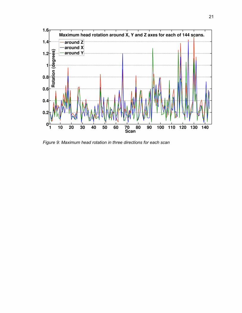
To study the effects of the translational motion on MEG data a 3D motion platform was

constructed (Figure 12). The platform was built with magnetically silent materials and

attached to the base of the Current Dipole phantom provided with the MEG unit by the

manufacturer (Figure 13).

a) Current Dipole Phantom

The Current Dipole phantom is a device and a tool allowing one to simulate a magnetic

brain signal in the scanner for quality assurance and troubleshooting purposes. The

phantom is MEG-compatible and made of magnetically silent materials (no

38

ferromagnetic ingredients), filled with a conductive medium (saline solution) and has 13

insertion holes to place a dipole for signal generation. The dipole is built with two wires

attached to the golden spherical electrodes and can generate a current within the

conductive medium of the phantom head. Figure 13 displays an image of the Current

Dipole phantom with a dipole labeled accordingly. Labels R, N and L point to the pins to

which three fiducial coils for head localization are attached (right (R) and left (L) pre-

auricular points and nasion (N)).

Figure 12: MEG 3D Motion Platform

Prior to obtaining any Current Dipole phantom recordings, the motion platform was

tested for magnetic noise or impurities and confirmed to be free of noise. Components of

the Current Dipole phantom, on the other hand, had become magnetically noisy due to

high magnetic field exposure in a 3T MRI scanner. These components are insulating

brown rubber O-rings within the phantom head. The large O-ring is situated between two

39

Phantom’s head hemispheres along the perimeter and 13 small O-rings insulate 13

holes in the base of the Phantom’s head. The insulating O-rings, large and small, have

brown color pigment that retained some magnetic field that was detectable by the MEG

scanner which led to noise contamination of the MEG data. Once all O-rings were

replaced, the phantom noise test improved substantially and became comparable to that

of the empty room. The phantom and the platform became suitable for clean MEG

recordings.

40

Figure 13: The Current Dipole Phantom with one dipole inserted into the phantom head

41

b) Data collection with motion

To investigate motion effects the motion platform with attached Current Dipole phantom

was operated manually in the magnetically shielded room with the motion precision

measurement of ± 1 mm in each direction along all three axes. Two data sets were

collected during three different days: unfiltered and filtered. Unfiltered data was raw

MEG data with no pre-acquisition or post-acquisition filters applied. Filtered data set was

recorded with 3rd gradient noise reduction, removed DC offset, and 1-40 Hz band width

filtering. These two different data sets allowed the separation of noise and artifact

reduction from the motion correction itself when a motion correction method is applied to

the data. Also, unfiltered and filtered data sets were chosen to be used in this study to

determine if motion correction methods are sensitive to the placement in the analysis

pipeline: before or after data pre-processing step. The directions and the amount of

phantom motion in the helmet were determined empirically such that the minimum

motion was 3 mm on the first day of recordings and 2 mm on the following two days. The

2 mm increment was chosen to match the minimum precision of the detection of the

fiducial head coils specified by the manufacturer. The MEG helmet and thus the sensor

array is symmetrical in the Left/Right directions (along Y axis) allowing only one of these

two directions to be used for the quantitative analysis. In this study the Left direction was

chosen (along the negative Y axis). The directions and the amount of phantom motion in

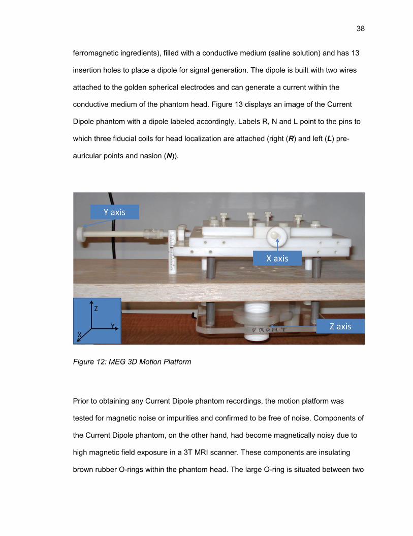
the helmet are listed in Table 1.

The amount of motion in each direction was based on the helmet shape and the

phantom head size which limited the left/right and front/back motion to 10 mm maximum.

The minimum motion was based on the head coils localization accuracy of 2 mm 13. The

head localization coils were mounted around the phantom circumference on the three

42

phantom pins representing nasion, left and right fiducial points (Figure 13). The phantom

was recorded with continuous head detection and localization using these three

localization coils. The current dipole was inserted into the phantom conductive medium

at (0, 0, 50 mm) point with respect to the center of the phantom head. The following

settings were recommended by the manufacturer as clinically relevant acquisition

parameters and used in this study to generate a measurable signal during each

recording:

- sinusoidal current with frequency of 7 Hz,

- peak voltage amplitude of 5 V,

- current amplitude in the range of 200 µA.

43

Table 1: Direction and extent of the Current Dipole phantom motion

Direction

Filtered

(mm)

Unfiltered

(mm)

Direction

Filtered

(mm)

Unfiltered

(mm)

LEFT (Y +) 3 n/a BACK (X -) 8 8

LEFT (Y +) 5 5 BACK (X -) 10 10

LEFT (Y +) 8 8 UP (Z +) 3 5

LEFT (Y +) 10 10 UP (Z +) 5 8

FRONT (X +) 3 n/a UP (Z +) 8 10

FRONT (X +) 5 5 UP (Z +) 10 20

FRONT (X +) 8 8 DOWN (Z -) 5 5

FRONT (X +) 10 10 DOWN (Z -) 10 8

BACK (X -) 3 2 DOWN (Z -) 15 10

BACK (X -) 5 5 DOWN (Z -) 20 20

The magnetic signal from the current dipole in the phantom was recorded without any

phantom motion on each day to obtain an ideal data set to be used in later quantitative

comparison between ideal vs. motion and motion corrected data. The construction of the

motion platform and use of the Current Dipole phantom in the motion study permitted

recordings of two data sets containing

- minimum background variance,

- known signal generator’s position and strength,

44

- precisely measured motion and its direction.

Thus the data sets can be used to study the motion correction results only, and should

permit a quantitative description of the motion correction methods.

II.B Motion correction performance and comparison

One of the goals of this study is to systematically and quantitatively evaluate the

performance of the SSS and GLM correction methods. Performance evaluation is

achieved by comparison of an ideal data set (data without motion) to the motion data

and to the motion corrected data and calculation of five assessment criteria: Percent-

Root-Difference (PRD), Pearson Product-Moment Correlation Coefficient (CC), Signal-

to-Noise Ratio (SNR), localization accuracy and signal coherence 29–33. Improvement or

deterioration of the corrected data were calculated as the difference or percent

difference between assessment values calculated for data with motion and for data

corrected for the motion.

II.C Motion assessment criteria

1) Percent-Root-Difference

Change in PRD normalized for DC offset was calculated in two steps:

_1YU %� = 0��% ∗ b∑ ;3�6<� 3� − <���J! 3�@ /43D0∑ ;3�6<� 3� − d�6<�eeeeeeee@ /43D0

Equation ( 22 )

45

∆_1Y %� = _1Y4J_=Ieeeeeeeeeeeee − _1Y=Ieeeeeeeeee Equation ( 23 )

In Equation ( 22 )

n is the total number of samples evaluated,

k is the channel number (the total number of channels was 272), 3�6<� is the channel recording for data without motion,

<���J! is the channel recording for data either with motion or corrected for the motion,

3�6<� 3� and <���J! 3� is the ith data sample for 3�6<� and <���J! data

respectively,

d�6<�eeeeeeee is the mean value of the channel recording for the 3�6<� data.

In Equation ( 23 ) the change in PRD, ∆PRD, was calculated in two steps, first finding an

average PRD for all channels (obtained in Equation ( 18 )), then subtracting average

PRD for data with motion correction (=I stands for motion correction) from the data

without the motion correction (4J_=I stands for no motion correction).

2) Pearson Product-Moment Correlation Coefficient

Change in CC was calculated in three steps, first calculating the kth channel CC, then

finding an average CC for all channels to obtain one per each data file, and then

determining the percent difference change between average CC with and without motion

correction:

46

ggU = IJ� 3�6<�, <���J!�3�6<�<���J! Equation ( 24 )

∆gg %� = 0��% − gg=Ieeeeeeegg4J_=Ieeeeeeeeeee ∗ 0��% Equation ( 25 )

In Equation ( 24 ) IJ� 3�6<�, <���J!� is the covariance between 3�6<� and <���J! data for channel

k; 3�6<�<���J! is the product of two standard deviations for the 3�6<� and <���J!

data respectively.

In Equation ( 25 )

gg=Ieeeeeee is averaged across all channels CC for data corrected for the motion,

gg4J_=Ieeeeeeeeeee is averaged across all channels CC for data containing the motion but not

corrected.

3) Signal-to-Noise Ratio

Change in SNR was calculated in three steps, first calculating the SNR for the kth

channel, then finding an average SNR for all channels per each data file, and last

calculating the difference between average SNR for motion corrected data and average

SNR for data without motion correction:

47

hi1U = 0�PJj0� k=J�3J4_l�66/=J�3J4/ m Equation ( 26 )

∆hi1 = hi1=Ieeeeeeeee − hi14J_=Ieeeeeeeeeeeee Equation ( 27 )

In Equation ( 26 )

=J�3J4_l�66/ is the variance of the motion free data segment,

=J�3J4/ is the variance of the data segment containing the motion (corrected or not).

Note: both segments were taken from the same channel recording and are of the same

length. SNR was calculated for each channel k and is proportional to the ratio of the

variances.

In Equation ( 27 )

hi1=Ieeeeeeeee is averaged across all channels SNR for the data corrected for the motion,

hi14J_=Ieeeeeeeeeeeee is averaged across all channels SNR for the data with the motion (prior to

correction).

4) Localization accuracy

Change in the dipole localization accuracy ∆� was calculated as:

∆� = n !=I − !3�6<��/ + #=I − #3�6<��/ + $=I − $3�6<��/ Equation ( 28 )

48

In Equation ( 28 ) !, #, $�=I are the Cartesian coordinates of the dipole signal localized in the data

corrected for the motion, !, #, $�3�6<� are the Cartesian coordinates of the dipole signal localized in the ideal

data.

In Figure 14 a sample of the current dipole localization procedure is shown. The

measured MEG data is shown in green as an overlap of all channels’ measurements

(the top left corner). The bottom left part of Figure 14 shows a contour map from all MEG

channels for one time instance that has a dipolar field distribution with maximum (in red)

and minimum (in blue). The right image is a schematic of the signal localization with a

resulting dipole (in red) with its (x, y, z) coordinates used in ∆o, localization accuracy,

assessment calculation.

49

Figure 14: Current Dipole Localization

5) Signal coherence

Signal coherence g!# was calculated as

g!# = �_!# l��/_!! l�_## l�

Equation ( 29 )

In Equation ( 29 ) _!# l� is the cross-spectral density between signal x (on one channel) and signal y (on

another channel) for frequency f in the same data segment,

50

_!! l� and _## l� are the auto-spectral densities of signal x and y respectively. Thus

coherence was calculated amongst all channels’ recordings for each motion data

segment. More about average coherence calculation can be found further in the section

II.C (6).

The first three criteria, PRD, CC and SNR, were applied to the raw and motion corrected

MEG data on a channel-by-channel base and then averaged across all channels.

Averaging is justified by comprehension that any phantom (or head) motion within the

helmet simultaneously affects all measurements on all channels.

PRD evaluates the accuracy and agreement between two data sets (smaller PRD

means more accurate result). CC measures linear similarity between two waveforms and

ranges from -1 to 1. CC ≈ 1 is a desired result for the motion corrected data. Changes in

SNR assess effects of motion correction on the data quality and noise level. Signal

coherence g!# evaluates the frequency and phase relations amongst all possible pairs

of two signals of the same MEG recording. Thus the signal coherence detects relative

changes in frequency and/or phase in the same MEG recording.

The ∆o criterion directly evaluates the ability of the motion correction method to change

the MEG recordings to the recordings that would have been measured without the

motion, allowing accurate localization of the source. The Current Dipole phantom

utilizes a dipolar source which is best localized with a Dipole Fitting method (MISL CTF

MEG™ DipoleFit was used in this study). The method starts with a user’s guess, a

51

knowledgeable estimate, for a possible number of the dipoles and their locations within

the spherical conductor, and calculates the forward solution for this estimate. The

method recursively adjusts the location and strength of the dipoles until a threshold in

the precision is met (MISL CTF MEG™ DipoleFit manual).

6) Average coherence calculation

Recently, various beamformer methods became popular in the MEG community for

signal localization and analysis. These methods are not suitable to localize temporally

coherent sources as these methods partly or entirely suppress or misplace such sources

34. Therefore signal coherence of the motion corrected data was investigated in this

study.

Signal coherence changes introduced by each motion correction method can be studied

with the last criterion signal coherence, g!#. This criterion evaluates signal correlation

among all channel recordings in the ideal and motion corrected data. For 272 channel

recordings there are 36856 possible combinations of channel-pairs. Default settings for

the Matlab function of the magnitude squared coherence, mscohere(x,y), were used on

each segment corrected for the motion (one segment per each file) and on each

equivalent segment from the ideal data set (Matlab: Release 2010a, The MathWorks,

Inc., Natick, Massachusetts, United States). Each channel-pair coherence of the motion

corrected data was evaluated against its ideal counterpart to establish if the coherence

difference is statistically significant with Welch’s t test on channel-pair-by-channel-pair

base. The resultant coherence matrix was thresholded by 0.85 (coherence ≥ 85% of the

maximum coherence) and only statistically significant coherence differences were

52

retained. The thresholded coherence was averaged across all pairs for each data set

and reported as the coherence strength. Another measurement of the signal coherence

is the number of the coherent links. The number of coherent links (for the thresholded

coherence) was evaluated in relation to the total number of links. The coherent fraction l

was calculated for each data set as

l = l3��6�6� & �q�6KqJ��6� IJq6�64I6 �34UK<�� �JKK3?�6 IJq6�64I6 �34UK Equation ( 30 )

In Equation ( 30 ) l3��6�6� & rℎtuvℎwxyuy zwℎutu{zu x|{}v is the sum of all the links

left after coherence strength was thresholded by 0.85 and only statistically significant

results were retained, <�� �JKK3?�6 IJq6�64I6 �34UK is the sum of all possible

coherence links.

The coherent fraction l was calculated for the motion corrected data on the time window

containing the motion and for the ideal data containing the same time segment.

Standard deviations were calculated for all assessment criteria as

hY = b 00 − 4 : !3 − !~�/ 43D0

Equation ( 31 )

53

In Equation ( 31 )

n is the total number of samples evaluated, !3 is the ith sample,

!~ is the mean value of all samples.

The analysis involved calculation of differences between ideal, motion and motion

corrected data thus requiring a combination of two or more SD. To combine two or more

SD a pooled variance was calculated as follows:

�JJ�6�/ = ∑ 43 − 0�3/U3D0∑ 43 − 0�U3D0 Equation ( 32 )

In Equation ( 32 )

k is the total number of SD to be combined,

3/ is the variance of the ith population,

n is the number of samples that were used to calculated each SD (for MISL CTF MEG™

DipoleFit method 60 Monte Carlo simulations were used to determine the confidence

volume and thus SD of the fit).

54

III. RESULTS

III.A Signal Space Separation vs. General Linear Modeling

Change in PRD was calculated for filtered and unfiltered data sets for the SSS and GLM

corrected data separately and compared against each other for each motion type as

∆_1Y�3ll = ∆_1Yhhh − ∆_1Y�P� Equation ( 33 )

In Equation ( 33 )

∆_1Yhhh is the change in PRD for the SSS motion corrected data,

∆_1Y�P� is the change in PRD for the GLM motion corrected data.

The resultant ∆_1Y�3ll was averaged across all motion types and reported in Table 2.

∆gg�3ll and ∆hi1�3ll were calculated similarly to ∆_1Y�3ll for each type of motion and

then averaged across all motion types. Change in the localization accuracy was

calculated in Equation ( 34 ) and averaged across all motion types and reported as

∆��dlleeeeeeee in Table 2.

∆��3ll = ∆��P� − ∆�hhh Equation ( 34 )

As a result, the positive values of ∆_1Y�3ll (or ∆gg�3ll or ∆hi1�3ll or ∆��3ll) point to

better accuracy performance of SSS compared to GLM and negative values show better

accuracy performance of the GLM correction.

55

Table 2 contains the summary on the comparison between SSS and GLM methods with

four assessment criteria used in the analysis.

Table 2: SSS vs. GLM motion correction methods comparison

SSS vs.

GLM

Aver

∆_1Y�3ll(%)

Aver

∆gg�3ll(%)

Aver

∆hi1�3ll Aver ∆��3ll (mm)

Unfiltered -427.8 -27.0 -3.4 1.6 ± 2.2 (p=0.003)

Filtered 22.5 6.6 -0.1 1.3 ± 1.4 (p=0)

For the unfiltered data set, ∆_1Y�3ll shows that the GLM correction performs better

than SSS correction on average by 427.8% by removing the noise and muscle artifacts

from the data (Table 2 and Figure 15). Both methods reduce PRD and thus improve data

accuracy because both methods remove motion noise and muscle artifact (due to the

manual motion platform operation) from the data.

56

Figure 15: Change in PRD; SSS vs. GLM comparison for the unfiltered data set

For the filtered data set, ∆_1Y�3ll provides a different view on both motion correction

algorithms: both methods lead to increase in PRD and hence to the reduction in data

accuracy such that the SSS correction performs better on average by 22.5% than the

GLM correction (Figure 16). This supports the FieldTrip requirement that GLM motion

correction cannot be applied at an arbitrary point in the analysis pipeline 12.

57

Figure 16: Change in PRD; SSS vs. GLM comparison for the filtered data set

Change in CC for the unfiltered data supports some or no improvement for the SSS

correction and an improvement up to about 54% for GLM correction. The GLM method

performs better than SSS on average by 27% (Table 2 and Figure 17). Change in CC for

filtered data shows a reverse picture: SSS correction gives little or no improvement in

CC when as GLM shows reduction in CC up to 8% (Figure 18). For filtered data set,

SSS performs better than GLM on average by 6.6% (Table 2 and Figure 18). All CC

results have a p-value ≤ 0.05.

58

Figure 17: Change in CC; SSS vs. GLM comparison for the unfiltered data set

Figure 18: Change in CC; SSS vs. GLM comparison for the filtered data set

59

Averaged ∆SNR shows some minor improvement for the unfiltered data for both motion

correction methods with the exception of one direction, downward, for the SSS

correction (Figure 19). The GLM performs better in improving ∆SNR on average by a

factor of 3.4 when compared to ∆SNR for the SSS correction (Table 2). For the filtered

data averaged ∆SNR is also improved by each method but by a smaller amount and with

the exception of the downward direction, which is expected as the phantom head is

moved away from all sensors simultaneously. Averaged ∆SNR is reduced for this

direction for both methods (Figure 20). For the filtered data set, GLM correction performs

only slightly better than the SSS correction on average by a factor of 0.1 (Table 2).

Figure 19: Change in SNR; SSS vs. GLM comparison for the unfiltered data set

60

Figure 20: Change in SNR; SSS vs. GLM comparison for the filtered data set

The next assessment criterion used is the localization accuracy with the Dipole Fitting

method, ∆r. For both data sets, unfiltered and filtered, ∆r is smaller for the SSS

correction method therefore yielding a better localization accuracy by SSS than GLM

(Figure 21 and Figure 22). The standard deviation bars for both filtered and unfiltered

data sets are ≤ 2.2 mm and are not included in Figure 21and Figure 22 for clarity.

61

Figure 21: Localization difference between ideal data and data corrected for the motion

with SSS and GLM for unfiltered data set

The SSS correction yields localization accuracy that on average is 1.6 ± 2.2 mm better

compared to the GLM method for the unfiltered data with a p-value of 0.002 (calculated

with two-sample Student t-test). For the filtered data set, the SSS method localization is

better on average by 1.3 ± 1.4 mm with a p-value of 4.68E-4 (Table 2 and Figure 22).

The localization accuracy for SSS is within 1 mm for both data sets with the exception of

the unfiltered data with motion to the back of the helmet which is within 2-3 mm.

Localization accuracy declines approximately linearly with the amount of motion for GLM

corrected filtered and unfiltered data, nevertheless permitting the localization

improvement by a factor of 2-4 (Figure 21and Figure 22).

62

Figure 22: Localization difference between ideal data and data corrected for the motion

with SSS and GLM for filtered data set

The last assessment criterion g!#, change in coherence strength, was calculated for

both data sets, unfiltered and filtered. For the unfiltered data set, the average coherence

strength and coherent fraction are reduced for both the SSS and GLM correction

methods when compared to the equivalent ideal data segment across all motion types

but only coherent fraction changes are statistically significant (Figure 23, Figure 24 and

Table 3).

63

Figure 23: Average Coherence Strength for all motions in the unfiltered data set

In Figure 23 above and Figure 24 through Figure 26 below red color is used to display

the change in coherence strength g!# and coherent fraction f for the SSS correction and

black color is used for GLM. The blue color is used for SSSsm (SSS smoothed) method

which is discussed below.

64

Figure 24: Average Coherence Fraction for all motions in the unfiltered data set

For the filtered data set, the GLM correction introduces a small increase in the

coherence strength (0.4% on average) and coherent fraction (8.2% on average) with

only the coherent fraction change statistically significant. For the SSS method the

average coherence strength and coherent fraction are both reduced in the filtered data

set by 0.2% and 12.6% on average respectively and these changes are statistically

significant (Figure 25, Figure 26 and Table 3).

65

Table 3: Change in signal coherence and its fraction for SSS, GLM and SSSsm

correction methods for the filtered and unfiltered data sets

UNFILTERED FILTERED

Method

Aver ∆

Fraction

(f)

Aver ∆

Coher

(g!#)

p-value

for f

p-value

for g!#

Aver ∆

Fraction

(f)

Aver ∆

Coher

(g!#)

p-value

for f

p-value

for g!#

SSS -0.257 -0.013 0 0.254 -0.126 -0.020 0 0

GLM -0.127 -0.013 0 0.257 0.082 0.004 0.003 0.154

SSSsm -0.027 0 0.218 0.171 0.385 0.024 0 0

66

Figure 25: Average Coherence Strength for all motion in the filtered data set

67

Figure 26: Average Coherence Fraction for all motion in the filtered data set

Further investigation of the SSS coherence and coherent fraction decrease indicates

that the SSS correction method introduces higher frequency components into the

corrected data which leads to apparent coherence reduction (Figure 27). In Figure 27

2.5 sec data segments for one channel recording for the ideal (in blue), and corrected for

motion by GLM (in red) and SSS (in green) are displayed. The SSS corrected data

shown in green color displays the largest deviation from the ideal segment shown in

blue.

68

Figure 27: Ideal data segment vs. the SSS, GLM and SSSsm corrected data segments

for one channel recording at the maximum extent of the motion

To enable true evaluation of the coherence changes and possible route for the SSS

improvement, the resultant SSS corrected data were subjected to an additional post-

processing step: data smoothing with local regression using weighted linear least square

and 2nd polynomial model: Matlab function smooth (Matlab: Release 2010a, The

MathWorks, Inc., Natick, Massachusetts, United States). This step is labeled as the

SSSsm method on all graphs in Figure 23 through Figure 27 and Table 3.

For the unfiltered data set, coherence analysis for SSSsm corrected data shows no

statistically significant changes in coherence strength or coherence fraction. For the

filtered data set, coherence analysis demonstrates statistically significant coherence

strength increase (on average by 0.024) and coherent fraction increase (on average by

69

38.5%) for the SSSmc method. Thus, under the assumption that the data smoothing

allows visualizing the true changes in the coherence strength and number of coherent

links, the SSS correction method introduces a statistically significant coherence increase

when applied to the filtered data.

III.B Motion correction method of choice and its limitations

Summarizing all the results for the SSS and GLM comparison with five assessment

criteria shows that SSS is the method of choice for the head motion correction

application because the method improves data accuracy, precision and source

localization fidelity. As well, the method is independent of its placement within the

analysis pipeline and works best for a filtered (pre-processed) MEG data. Data filtering

prior to any analysis is a common practice in the MEG field. The SSS corrected data can

be safely used for further analysis such as source localization. SSS yields better

localization precision than GLM.

It appears that one of the drawbacks of the SSS method is change of the signal

coherence, which is especially evident for the filtered data set. The change in the

coherence strength and the number of the coherent links can be due to introduction of

additional frequency components into the corrected data as seen in Figure 27 or due to

change of the phase component in the corrected data.

Another drawback is data overfitting. In the MISL CTF MEG™ SSS method the number

of expansion terms is predetermined and fixed and must be greater than the number of

MEG channels 13. The fixed number of the expansion terms and the choice of the

70

regularization method lead to introduction of the higher frequency components into the

motion corrected data that initially only contained low frequency signal. For relatively

simple recordings such as from one current dipole source of 7 Hz the overfitting leads to

signal ringing in the corrected data (Figure 27). Thus the choice of the number of the

expansion terms should not be predefined but rather data driven. Also the coherence

change can possibly be caused by the assumption that the MEG data are recorded over

a perfectly spherical shell, when as the sensor array shell is more ellipsoidal in shape.

III.C Theoretical approach to improve Signal Space Separation

method

The SSS method is based on the spherical harmonics expansion that includes both

radial �>�>0 & �� and angular A�= B, C� components. The angular component is the

surface spherical harmonic functions. Harmonic functions are solutions of the Laplace’s

equation when solved via separation of variables. It has been shown for a three-

dimensional case that Laplace’s equation is separable in eleven different orthogonal

coordinate systems 35. The most general amongst these coordinate systems is an

ellipsoidal coordinate system with one of its degenerate forms being a spherical

coordinate system 36. The surface spherical harmonic functions are defined over a

spherical surface. In general, surface harmonic functions are functions whose domains

are surfaces, thus the choice of the surface harmonics is dictated by the surface to be

modeled. In case of the MEG data, the surface to be modeled is the sensor array shape

as it is the surface of measurements.

The spherical harmonics expansion is chosen in the SSS method owing to the spherical

71

harmonics advantages such as

- any function on a sphere can be represented as a linear combination of the surface

spherical harmonics to any degree of the precision,

- spherical harmonics are orthogonal with respect to the integration over a sphere, thus

allowing one to obtain a unique function representation,

- analytical formulation of the spherical harmonics transformations under translation is

known and available 21, 37,

- rotation of the function represented with spherical harmonics is achieved by re-

adjustment of the expansion coefficients (multipole moments); new rotated coefficients

are calculated as a linear combination of the old ones for each given band limited by the

degree �; spherical harmonics are invariant under the rotation 38,

- spherical harmonics can be arrange from low to high spatial frequencies representing

the function details from coarse to fine 35.

These advantages will reduce or vanish if the surface is only approximately spherical or

not spherical at all.

To improve the SSS motion correction method the sensor array shape of the MISL CTF

MEG™ scanner was investigated in this study.

a) Sensor array shape and its fit approximation

Each MEG sensor location is described by three Cartesian coordinates related to the

head coordinate system defined by the three fiducial coils attached to the subject’s or

phantom head. Thus the sensors coordinates vary from subject to subject or different

phantom positions inside the helmet due to the difference in the location of the origin.

72

The coordinates are calculated and recorded with MEG data collected during the

recording session. These coordinates were extracted and analyzed in Matlab (Matlab:

Release 2010a, The MathWorks, Inc., Natick, Massachusetts, United States) with the

Levenberg–Marquardt surface fitting algorithm. The algorithm was chosen for its

simplicity and availability, and is sufficient for simple surfaces such as the MEG sensor

array for surface comparison. Levenberg–Marquardt algorithm solves non-linear least-

square problem by minimizing the difference between the data and each iterative

solution.

To examine the effect of different sensor array coordinates on the surface fitting, two

different data sets were chosen for the sensor array shape analysis:

- real subject MEG recording,

- Current Phantom MEG recording.

The goal of any approximation or expansion is to find a data representation such that

this representation is as close to the initial data as possible and yet it is simpler and

easier to handle or analyze than the original data. Thus representing the sensor array

shape with a spherical surface is the simplest approximation. Because Laplace’s

equation is also separable in the spheroidal and ellipsoidal coordinate systems, the

surface fitting with a spheroid and ellipsoid was examined here.

The origin of the coordinate system for the Current Phantom was very close to the

geometrical center of the array and the coordinate axes were leveled in relation to the

axes of symmetry of the sensor array. In contrast, the origin of the coordinate system for

73

the subject was less centered and the coordinate axes were tilted due to the locations of

the left and right pre-auricular points and the nasion point (Figure 28). These differences

lead to very different fit results between these two data sets for all fits: spherical,

spheroidal and ellipsoidal.

Figure 28: Subject and Phantom sensor arrays coordinates & orientation

In Figure 29 below the fitting results are shown. The blue dots represent the sensors

locations stretched along Z axis (the Z coordinate was squared to allow fitting to an

equation without square root operation). The Phantom column of Figure 29 depicts

clearly that the phantom sensors coordinates have better fit with all three surfaces than

that for the subject. In the Table 4 R-square is a statistic measure describing the

goodness of fit or how much of the data was explained with the fit correctly. The

Phantom spherical fit has R-square of 86.48% which is only slightly worse than that for

the spheroidal fit of 86.85%; as it was expected, the ellipsoidal fit describes the sensor

array shape best resulting in R-square of 93.11% (Table 4).

74

Figure 29: Spherical, spheroidal and ellipsoidal surface fitting for Phantom and subject

recordings

The real subject fit results are less precise with R-squares of 59.64% for spherical fit,

70.34% for the spheroidal and 80.56% for the ellipsoidal (Table 4). Spheroidal surface in

75

place of the spherical can be a reasonable improvement of 10.22% in modeling the array

shape for the real subject’s data and of 0.37% for the phantom data. Thus the spheroidal

coordinate system can provide a potential improvement in MEG data modeling.

Measurements over a spheroidal surface can be well represented by spheroidal surface

harmonics expansion. It appears that using spheroidal surface harmonics for the MEG

data modeling in the motion correction can improve the data expansion and its

approximation, thus the precision and accuracy of the head motion correction itself.

76

Table 4: Numerical results for spherical, spheroidal and ellipsoidal surface approximation

for Phantom and subject recordings

Fit type & fitting equation

Coefficients (mm)

R-square

Subject Spherical a=150.3 59.64%

Phantom $/ = </ − !/ − #/ a=121.6 86.48%

Subject Spheroidal

a=134.4

c=172.1

70.34%

Phantom

$/ = I/ − NI<O/ ;!/ + #/@

a=122.8

c=118.6

86.85%

Subject

Ellipsoidal

a=146.5

b=119.2

c=178.7

80.56%

Phantom

$/ = I/ k0 − N!<O/ − N#?O/m

a=130.7

b=114.6

c=120.7

93.11%

77

b) Transformation from Cartesian to spheroidal coordinate system

The MEG sensor coordinates are available in Cartesian coordinate system (CTF MEG

Coordinate System) and shown in Figure 6. A coordinate transformation from Cartesian

to spheroidal (oblate or prolate) must be performed prior to the spheroidal harmonics

expansion. Both oblate and prolate spheroids can be used for modeling the MEG sensor

array shape. As seen in Table 4, the spheroidal fit for the subject yields a prolate

spheroid with c > a and an oblate spheroid for the phantom with c < a. The spherical

coordinate system is a special case of the spheroidal coordinate system when the

spheroid eccentricity is zero (a = c).

The spheroidal coordinate system is constructed by rotation of an ellipse around one of

its axes of symmetry (major or minor) aligned along the Z axis. Rotation around the

major semi-axis results in the prolate spheroidal coordinate system with its unit domain a

football shape spheroid (Figure 30) 39–41. Rotation around the minor semi-axis results in

the oblate spheroidal coordinate system with the unit domain of the Earth shape

spheroid (Figure 30) 39–41. Oblate and prolate coordinate systems are described by three

orthogonal coordinates �, �, C� such that � ϵ [0, ∞∞∞∞], � ϵ [-π/2, π/2] and C ϵ [-π, π]. In

all three coordinate systems, spherical and two spheroidal, C is the azimuthal angle (or

longitude, the angle along the equatorial plane). The coordinate surfaces for the

coordinate C are planes.

The coordinates � are represented by confocal ellipses; � differs between oblate and

prolate coordinate systems and can be thought of as an analog (but not the same) of the

radial coordinate in the spherical coordinate system. The coordinates � are reduced

78

latitudes (angular coordinates along the North-South direction) 42. These coordinates are

represented by a set of hyperboloids.

There are other possible choices of three coordinates for the spheroidal coordinate

systems but �, �, C� is preferred here as the solution to the Laplace’s equation is

separable only for these coordinate choice 43.

Figure 30: Oblate (left column) and prolate (right column) spheroids and their coordinate

systems in X-Z plane for φ = 0

79

The simplest representation of the relation amongst coordinates of the three coordinate

systems, Cartesian, spheroidal and spherical, can be found in Equation ( 35 ) through

Equation ( 37 ) where the plus sign represents equations for the oblate spheroidal

coordinate system and the minus sign is for the prolate 44:

! = ��/ ± '�,J/ K34 ��IJK C� = �K34 B�IJK C� Equation ( 35 )

# = ��/ ± '�,J/ K34 ��K34 C� = �K34 B�K34 C� Equation ( 36 )

$ = �IJK �� = �IJK B� Equation ( 37 )

In Equation ( 35 ) - Equation ( 37 )

� is the complement of the reduced colatitude, i.e. 900 minus the angle measured

between the equatorial plane and the positive direction of the Z axis,

'J/ = 0 − NI<O/is the eccentricity of the oblate reference spheroid,

with < and I its equatorial and polar radii respectively,

'�/ = 0 − N<IO/ is the eccentricity of the prolate reference spheroid.

c) Spheroidal harmonics expansion

It was realized by Jekeli, C. 1987 43, that the equation for calculation of the spherical

harmonics expansion coefficients does not involve a spherical surface explicitly and can

80

be applied to any other surfaces that can be projected onto a spherical one, i.e. have

unique set of coordinates in the spherical coordinate system (Equation ( 38 )).

<�= = 0�� � . B, C�MA�= B, C� �M Equation ( 38 )

Equation ( 38 ) was adapted to current notation from Jekeli, C. 1987 43, and shows

integration over the surface M with the surface spherical harmonics A�= B, C�. In the

case of MEG measurements, . B, C�M is a set of measurements collected over the

sensor array surface which is better modeled by a spheroidal surface. The collection of

all expansion coefficients {<�=} is called the data spectrum. The spectrum difference is

significant between different surface measurements, especially for a higher degree of

expansion 43. Thus replacing the spherical surface with the spheroidal improves the

accuracy of the expansion of MEG measurements. The surface spherical harmonics

A�= B, C� can be replaced with the surface harmonics in the spheroidal coordinate

system A�= �, C� allowing computation of the expansion coefficients that are better

representatives of the measured data (Equation ( 39 )).

<�= = 0�� � .K��l<I6A�= �, C� �M Equation ( 39 )

The MISL CTF MEG™ scanner is equipped with reference magnetometers situated at

some distance above the primary gradiometers and predominantly collecting

environmental noise measurements. These measurements are used in the noise

reduction step called a 3rd order synthetic gradiometer formation. Based on the reference

81

channels’ locations the 3rd order synthetic gradiometery allows the removal of the

majority of the signal measured outside of the MEG helmet. This is a direct (based on

real measurements) and robust method to remove external signals from MEG data.

Thus it can be used in place of the signal space separation step that separates all

measured data into external and internal signals and drops the external signals out of

the measurements. If the 3rd order synthetic gradiometery is applied to raw MEG data,

mainly only internal signals are retained in the data. These data now can be expanded

with the internal spheroidal harmonic functions only. The magnetic scalar potential . in

the oblate spheroidal harmonics expansion is shown in Equation ( 40 ).

. �, �, C� = 0�� : : <�=6 ��= 3�/'���= 3?/'� A�= �, C��=D>�

E�D�

Equation ( 40 )

In Equation ( 40 )

<�=� are the spheroidal expansion coefficients,

��= 3�/'���= 3?/'� are the expansion components equivalent to the radial part N1�O��0 in the internal

spherical harmonics expansion,

? is the semi-minor axis,

��= ∗� are associated Legendre functions of the 2nd kind,

A�= �, C� are the spheroidal surface harmonics.

The magnetic scalar potential . in the prolate spheroidal harmonics expansion can be

derived from the Laplace’s equation in the oblate coordinate system by converting

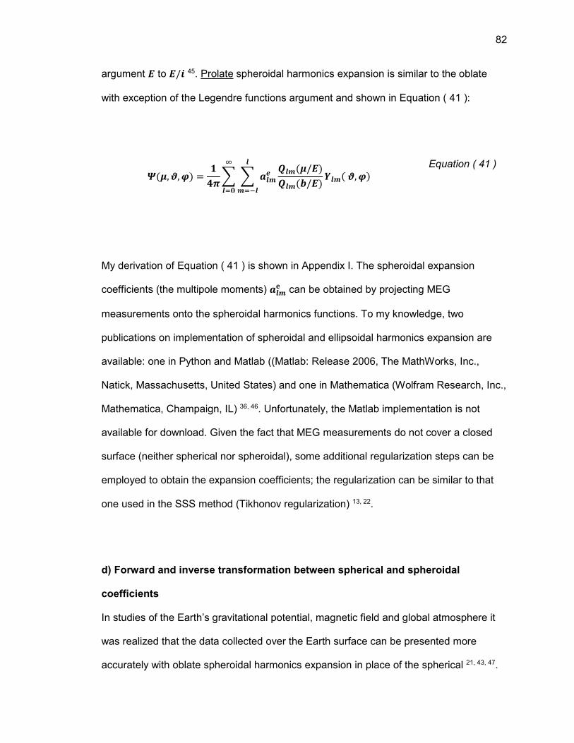
82

argument ' to '/3 45. Prolate spheroidal harmonics expansion is similar to the oblate

with exception of the Legendre functions argument and shown in Equation ( 41 ):

. �, �, C� = 0�� : : <�=6 ��= �/'���= ?/'� A�= �, C��=D>�

E�D�

Equation ( 41 )

My derivation of Equation ( 41 ) is shown in Appendix I. The spheroidal expansion

coefficients (the multipole moments) <�=� can be obtained by projecting MEG

measurements onto the spheroidal harmonics functions. To my knowledge, two

publications on implementation of spheroidal and ellipsoidal harmonics expansion are

available: one in Python and Matlab ((Matlab: Release 2006, The MathWorks, Inc.,

Natick, Massachusetts, United States) and one in Mathematica (Wolfram Research, Inc.,

Mathematica, Champaign, IL) 36, 46. Unfortunately, the Matlab implementation is not

available for download. Given the fact that MEG measurements do not cover a closed

surface (neither spherical nor spheroidal), some additional regularization steps can be

employed to obtain the expansion coefficients; the regularization can be similar to that

one used in the SSS method (Tikhonov regularization) 13, 22.

d) Forward and inverse transformation between spherical and spheroidal

coefficients

In studies of the Earth’s gravitational potential, magnetic field and global atmosphere it

was realized that the data collected over the Earth surface can be presented more

accurately with oblate spheroidal harmonics expansion in place of the spherical 21, 43, 47.

83

Since then, a transformation between spherical and oblate spheroidal harmonics was

studied and analytical solutions developed 43, 48. The transformation between spherical

and spheroidal expansion coefficients can be used for the SSS motion correction

method improvement. The SSS method corrects for the motion by adjusting the

spherical harmonics expansion coefficients for rotation and translation, which is a

simpler approach than adjusting the spheroidal harmonics expansion coefficients.

The exact transformation between oblate spheroidal and spherical coefficients is based

on the relation between solid spheroidal and solid spherical harmonic functions and can

be found in the equations (24) and (25) of Jekeli, C. 1988 43. The equations are included

below in the present notation as Equation ( 42 ) and Equation ( 44 ):

_�|=| N3 �'O A�= �, C� == −0�=3� /� + 0�/� ∙∙ : /� − /U�!U! � − U�! ��= /� − �U + 0� � − /U − =�! � − /U + =�!�0 /9

�UD�∙ N�'O�>/U A�>/U,= B, C�

Equation ( 42 )

In Equation ( 42 )

_�|=| N3 �'O A�= �, C� are solid spheroidal harmonic functions,

_�|=| N3 �'O are associated Legendre functions of the 1st kind,

3 is the imaginary number,

� and �= are defined below in Equation ( 43 ).

84

� = � − |=|/ <4� �= = �0. �, = = ��. \, = ≠ � � Equation ( 43 )

N�'O� A�= B, C� = −0�=3� ��= /� + 0� � + =�! � − =�!�0 /9 : /�>/U � − U�! /� − /U + 0�! U! ∙�UD�∙ _�>/U,|=| N3 �'O A�>/U,= �, C�

Equation ( 44 )

In Equation ( 44 ) N�'O� A�= B, C� are solid spherical harmonic functions.

In Equation ( 42 ) through Equation ( 44 ): � ≥ �, −� ≤ = ≤ � , 0 ≤ U ≤ �.

The transformation between the spherical and spheroidal expansion coefficients is

based on the boundary differences described by the different coordinate systems in

Equation ( 39 ), and on the fact that the spheroidal coordinate system reduces to

spherical when the eccentricity of the reference spheroid is reduced to zero 49.

Improvement of the SSS method is based on the spheroidal harmonics expansion in the

appropriate (oblate or prolate) coordinate system applied to the 3rd gradient noise

reduced MEG data. Then, the spheroidal coefficients obtained are coefficients

describing the internal signals: signals recorded primarily from the helmet volume. These

spheroidal coefficients can be converted to their spherical equivalents for the motion

correction by Equation ( 45 ). I derived Equation ( 45 ) from three equations (16), (18)

85

and (25) of Jekeli, C. 1988 43. This equation allows one to calculate the spherical

harmonics coefficients <�= K from the oblate spheroidal coefficients <�>/U,= 6 .

<�= K = ��= � + =�! � − =�!�0 /93��0 /� + 0�0 /9 ∙ +'1,��0 ∙ : /� − �U + 0�/�>/U � − U�! /� − /U + 0�U! ∙ <�>/U,= 6��>/U,|=| N3 ?'O

�UD�

Equation ( 45 )

In Equation ( 45 )

1 is the radius of the reference sphere, i.e. the auxiliary sphere tangent to the spheroid,

��>/U,|=| N3 ?'O are the associated Legendre functions of the 2nd kind.

The oblate and prolate coordinate systems are similar but rotated by 900 in relation to

each other (Figure 30). This symmetry allows coordinate systems conversion from

oblate to prolate by multiplying the spheroid eccentricity ' by 0 39 in all equations 45. Thus

Equation ( 45 ) can be converted to an equation for calculation of the spherical

harmonics coefficients <�= K from the prolate spheroidal coefficients <�>/U,= 6 by converting

��>/U,|=| N3 ?'O to ��>/U,|=| N?'O and N'1O��0 to N '31O��0

.

Corrected (for motion) spherical harmonics coefficients should be converted back to the

oblate (or prolate) spheroidal coefficients prior to signal reconstruction.

Equation ( 46 ) was borrowed from Jekeli, C. 1988, and adapted to present notation 43.

This equation converts spherical coefficients <�>/U,= K to the oblate spheroidal <�= 6 :

86

<�= 6 = ��|=| +3 ?', 3��0/� : /� − U�!U! � − U�!�UD� � �= /� − �U + 0� � − /U − =�! � − /U + =�! +1',�>/U�0 <�>/U,= K

Equation ( 46 )

Similarly,

Equation ( 46 ) can be converted to an equation for calculation of the prolate spheroidal

harmonics coefficients <�= 6 from the spherical <�>/U,= K by converting ��|=| N3 ?'O to

��|=| N?'O and N1'O�>/U�0 to N31' O�>/U�0

.

Another drawback of the SSS motion correction method was data overfitting: the total

number of the expansion terms is fixed and larger than the number of sensors

introducing higher frequency components into the corrected data. To facilitate a data-

driven choice of the total number of the expansion terms the Orthogonal Matching

Pursuit method (OMP) can be used to expand an MEG recordings with OMP basis

vectors 50. OMP is a sparse data approximation method based on finding the best data

representation with a given set of basis vectors such that the total number of the

projections (or coefficients) is minimized. This method is applicable to sparse data: the

degrees of freedom of the data are proportional and smaller than the total number of

measurements. The OMP method is built on the fact that the set of basis vectors (called

the OMP dictionary) is over-complete and redundant, i. e. the set combines more than

one orthogonal basis set. The resultant dictionary is not orthogonal but provides a wider

choice of the basis vectors to represent the signal. Most real signals, including MEG, are

not stationary and vary as a function of time and/or frequency. MEG signal can be a

87

smooth slow varying signal or a sharp and abruptly changing signal, thus, having a wider

choice of basis vectors helps better signal representation. Because the dictionary is not

orthogonal, the signal has no unique decomposition in this dictionary but a best (sparse)

representation can always be chosen. The advantage of using a non-orthogonal over-

complete set of basis vectors is to allow sparse signal representation, which is a method

of dimensionality reduction of the data.

The Orthogonal Matching Pursuit method was applied to three pseudo-randomly chosen

channels (# 50, 100, 200) in four different phantom recordings and one real subject MEG

recording. The OMP dictionary was built for 600 data samples with two subdictionaries:

sine waves and discrete cosine transform-II waves. The Matlab command line is

wmpdictionary (600, 'lstcpt', {'dct','sin'}). The resultant dictionary has 900 basis vectors.

Investigation of the four phantom recordings with the OMP method showed that the

phantom recordings can reliably be represented with 25 OMP coefficients among which

only 3 to 8 coefficients were the largest (with the amplitude of 2-4 order of magnitude

larger than the rest) with the Pearson's linear correlation coefficient ≥ 99% and p-value

of zero. Because this OMP dictionary is a set of sine and cosine waves and spherical (or

spheroidal) harmonic functions are also a combination of sine and cosine waves, it is

reasonable to assume that the determined number of OMP coefficients is a sensible

estimate of the total number of the spherical (or spheroidal) harmonics terms needed to

capture the full dimensionally of the phantom MEG signal.

88

Investigation of the real subject MEG recordings (resting state scan) with the OMP

method showed that a reliable OMP representation is archived with 100-150 coefficients

with the Pearson's linear correlation coefficient ≥ 98% and p-value of zero (Figure 31).

Figure 31: MEG signal dimensionality with the Orthogonal Matching Pursuit method

In Figure 31 MEG signal dimensionality plot was obtained with the first 19 seconds of the

resting state recording of a randomly selected MEG data from Head Trauma Study (IRB

# 00014350). A number of OMP fits was calculated for each second and each channel

starting with 30 and up to 150 expansion terms. These fits were compared to the original

data with Pearson's linear correlation coefficient. The resultant correlation coefficients

were first averaged across all 19 seconds and then the minimum and maximum

correlation coefficients were determined for each set amongst all channels.

89

IV. DISCUSSION

In the present study I investigated the amount and extent of the head motion during

MEG recording sessions with 80 healthy subjects and supported the previously known

knowledge of the downward direction due to slouching motion in the scanner 14. I also

showed that the rotational motion was quite negligible amongst 80 subjects and had no

preferred direction of the rotation. This is probably due to the fact that the helmet shape

is made to follow a larger head shape with a cutout for the face and any extreme head

rotation in the helmet will obstruct the subject’s field of view. The results of the

investigation led to the construction of a 3D motion platform to simulate translational

motion in the scanner and enable to collection of a variety of motion data under

prescribed conditions for the motion correction analysis.

The head motion correction problem has been previously addressed with a number of

offline head motion correction algorithms amongst which the GLM and SSS methods

were determined to be the most useful and available 12, 13, 17, 18, 51. These methods were

previously evaluated to determine their ability to remove or reduce head motion

confounds in MEG data. However, these two methods were not studied in depth from

the point of data quality or compared to each other in well-controlled but still realistic

settings. In this project the GLM and SSS methods were thoroughly studied,

quantitatively and qualitatively evaluated and compared to each other with the help of

the Current Dipole phantom (provided by the manufacturer) and the 3D motion platform I

designed and developed for this study.

90

The results of this comparison showed that the GLM method better improves signal

accuracy, linear similarity and SNR than the SSS method when applied to the raw MEG

recordings. The GLM advantage over the SSS when applied to raw the unfiltered data is

due to its better ability to reduce motion and muscle artifacts: moving signals produce

DC offsets and fluctuations in the data, and manual operation of the motion platform

introduce a detectable muscle artifact into the recordings. GLM reduces the total number

of the coherent links on average by 12% while SSS reduces the total number of the

coherent links on average by 25%, without any statistically significant changes in the

signal coherence strength for both GLM and SSS when applied to the raw MEG

recordings. Thus GLM generally does not change signal coherence.

For filtered data sets the SSS method performs better than GLM by improving the signal

accuracy and linear similarity of the data; SSS slightly reduces SNR when compared to

the GLM SNR. Reduction of SNR points to the noise level increase in the corrected data.

SSS reduces the coherence strength and the total number of the coherent links

(statistically significantly) in the filtered data set, while the GLM method introduces no

statistically significant changes in the coherence.

For both filtered and raw data sets the SSS method has better localization accuracy than

GLM. The SSS correction yields excellent localization accuracy (within 1-3 mm) and it is

independent of the amount of the motion. The localization accuracy within 1 mm agrees

with the results from Wilson, 2004 13. This accuracy appears to be superior to that of the

8.5-21.3 mm range in accuracy reported by Medvedovsky and colleagues for motions up

to 6 cm corrected with two different SSS implementation methods 52. The SSS and tSSS

91

(Spatiotemporal Signal Space Separation) methods have been implemented by Elekta

Neuromag® TRIUX™ 18. For better comparison between Medvedovsky and this study

an average localization error for motions < 3 cm was calculated from Table 1 of the

aforementioned article (Medvedovsky: Localization error and noise at deviant head

positions 11). These averaged localization errors are larger than those for the MISL CTF

MEG™ SSS implementation and are

- 9.2 ± 4.6 mm for the SSS method implemented with Elekta,

- 8.8 ± 3.3 mm for the tSSS method implemented with Elekta.

As a result of this investigation it was determined that the SSS method performs better

than the GLM method, especially when applied to the pre-filtered data sets by directly

correcting for the head motion and resulting in excellent signal localization independent

of the amount of the motion at least for up to 2 cm motions.

The possible limitations and assumptions of the SSS method were studied and

discussed, and some possible drawbacks were determined. One of these drawbacks is

the change in signal coherence. The SSS method changes coherence strength and the

number of the coherent links when the corrected data compared to its ideal counterpart.

Coherence changes can be explained by introduction of the additional frequency

components into the corrected data and/or by signal phase changes due to the spherical

harmonics rotation and translation transformations (as a part of the motion correction

algorithm).

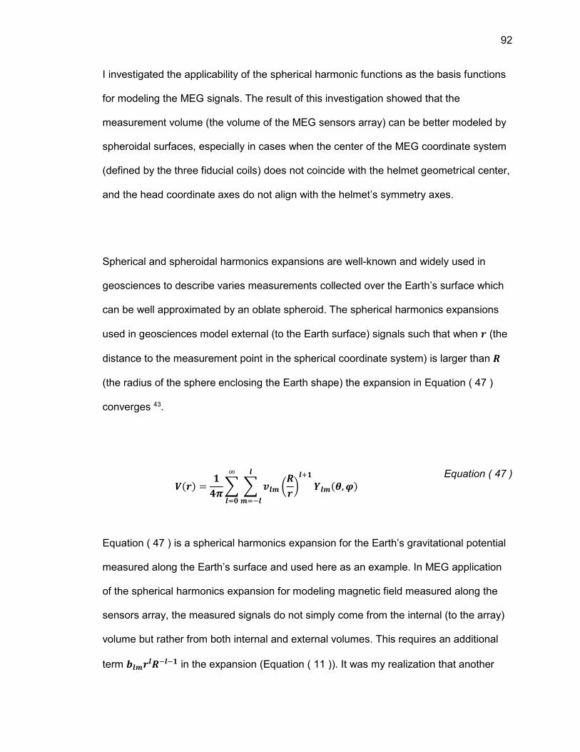
92

I investigated the applicability of the spherical harmonic functions as the basis functions

for modeling the MEG signals. The result of this investigation showed that the

measurement volume (the volume of the MEG sensors array) can be better modeled by

spheroidal surfaces, especially in cases when the center of the MEG coordinate system

(defined by the three fiducial coils) does not coincide with the helmet geometrical center,

and the head coordinate axes do not align with the helmet’s symmetry axes.

Spherical and spheroidal harmonics expansions are well-known and widely used in

geosciences to describe varies measurements collected over the Earth’s surface which

can be well approximated by an oblate spheroid. The spherical harmonics expansions

used in geosciences model external (to the Earth surface) signals such that when � (the

distance to the measurement point in the spherical coordinate system) is larger than 1

(the radius of the sphere enclosing the Earth shape) the expansion in Equation ( 47 )

converges 43.

� �� = 0�� : : ��= +1�,��0 A�= B, C��=D>�

E�D�

Equation ( 47 )

Equation ( 47 ) is a spherical harmonics expansion for the Earth’s gravitational potential

measured along the Earth’s surface and used here as an example. In MEG application

of the spherical harmonics expansion for modeling magnetic field measured along the

sensors array, the measured signals do not simply come from the internal (to the array)

volume but rather from both internal and external volumes. This requires an additional

term ?�=��1>�>0 in the expansion (Equation ( 11 )). It was my realization that another

93

important difference between spherical harmonics expansion for Earth’s data and

spherical harmonics expansion for MEG data is that the external term ��= N1�O��0 in

Equation ( 47 ) becomes internal term <�=�>�>01� in Equation ( 11 ). The reason for this

re-assignment is that the spherical harmonics expansion for the MEG internal term must

diverge when � → � because the magnetic scalar potential becomes infinite next to the

source 17. Similarly, the MEG external term must diverge when � → ∞ because the

magnetic scalar potential should also describe sources distant from the origin 17. My

understanding is that the same re-assignment can be applied to the spheroidal

harmonics expansion, i.e. external term of the Earth’s data spheroidal expansion can be

used to represent the internal term in the MEG data expansion.

Another analytical contribution of this study is to reduce the computational load of the

spheroidal expansion by realizing that the signals from the external sources can be

removed by the 3rd order synthetic gradiometery applied to the MEG data prior to the

motion correction. The 3rd order synthetic gradiometery step will remove the majority of

measurements from the external (to the MEG helmet volume) sources, thus yielding the

signal separation into two subspaces unnecessary.

It was proposed in this study to replace the spherical harmonics expansion with the

oblate (or prolate) spheroidal harmonics expansion to improve the data representation

fidelity prior to the motion correction (Equation ( 40 ) and Equation ( 41 )).

94

One of the advantages of using spherical harmonics as the basis functions is well

developed analytical and practical solutions for the functions transformation between

different coordinate system’s origins. These analytical and practical solutions have

relatively simple forms and are computationally robust 38, 37, 53. In order to preserve the

simplicity of the spherical harmonics application in the SSS motion correction method, a

forward and inverse conversion between spherical and spheroidal (both oblate and

prolate) expansion coefficients were obtained Equation ( 45 ) and Equation ( 46 ).

Thus, the proposed, improved SSS method derived in this work will consist of the

following steps:

- determine the shape and size of the best spheroidal fit (oblate or prolate) for a given

MEG data,

- obtain oblate (or prolate) spheroidal harmonics expansion of the data,

- convert the spheroidal expansion coefficients to their spherical equivalents,

- perform the head motion correction on the spherical internal expansion coefficients,

- convert the corrected spherical coefficients back to the spheroidal coordinate system,

- and reconstruct MEG recordings with the new spheroidal coefficients (corrected for the

motion).

The choice of the total number of the expansion terms was addressed with the

investigation of the MEG signal dimensionality with the OMP method. As was expected,

the Current Phantom MEG recording could be described reliably with a small number of

independent terms, 25 coefficients, while in contrast, a subject’s MEG recording needs

100 to150 OMP coefficients to have a reliable decomposition for all channels. The

95

finding of 100-150 terms supports the result found by S. Taula, 2004 with the total MEG

brain signal dimensionality of less than 200 and by S. Taula, 2005 of less than 150 17, 20.

In the future study a larger number of resting state and evoked response MEG

recordings should be investigated across various population of subjects to determine an

average range of the MEG signal dimensionality.

In the future work the application of the spheroidal harmonic functions to MEG head

motion correction method should be implemented based on the provided analytical

solutions in this study and tested with phantom and real MEG recordings containing

head motions. The results should be compared to the currently existing motion

correction methods in a similar manner. The computational load of the proposed method

should also be evaluated to justify the possibility of the method to be used in the real

clinical settings.

96

V. CONCLUSION

Magnetoencephalography is a non-invasive brain imaging technique enabling the

recording of the changing magnetic field from a living brain. It is a direct measurement of

the magnetic field produced by a large number of the brain neurons’ electrical currents.

This magnetic field while very small experiences minimum attenuation and distortion by

the head tissues due to the magnetic permeability of the soft tissues (water equivalent

tissues) being close to that of the vacuum (�� = �� × 0�>� i/�/) 2. The minimum

distortion of the magnetic field is a great advantage over an electric field of the same

neuronal activity as the electric field is highly dependable on the tissues’ electric

conductivities which vary from tissue to tissue and are usually hard to measure in a living

brain. Because the major detectors in a modern MEG scanner are SQUIDs, the

detectors must be super-cooled below the critical temperature to allow Niobium to

become super conductive. The drawback of such arrangement is that these detectors

must reside in a cryogenic environment of a Dewar and cannot be directly placed on a

scalp. A modern MEG head helmet must accommodate a variety of the head shapes

and sizes and thus permits some head motion in the relation to the detectors.

The goals of this study were to investigate and evaluate the head motion problem and

two head motion correction algorithms in magnetoencephalography with an aim to

improve an existing method or to develop a new approach. The head motion problem is

a well-recognized and addressed MEG problem 11–14, 16, 17, 20, 22, 23. There are two most

used head motion algorithms, GLM and SSS, which are commercially implemented,

studied and widely used for the head motion correction. However, these methods were

only studied from the point of view of the localization and statistical accuracy and there

97

are no systematic and quantitative studies that looked at the effects of these motion

correction methods on the data quality and/or compared these two methods to each

other to establish advantages and limitations. My work represents the first quantitative

study in this area.

I concluded that the SSS motion correction method yields better localization accuracy

and better data quality improvement than the GLM method when applied to the pre-

filtered MEG recordings. The SSS method has been further investigated and a route for

improvement of the method has been proposed. This route uses oblate (or prolate)

spheroidal harmonics expansion in place of the spherical harmonics expansion and still

preserves the simplicity of the translation and rotation transformations of the spherical

harmonic functions. The preservation is achieved via forward and inverse spherical to

spheroidal expansion coefficients transformations and analytical equations for these

transformations are presented in this study. Such that the motion correction can still be

performed on the spherical harmonics functions. I developed and described this new

method herein. Future work will include robust testing of the new algorithm with phantom

and real MEG recordings to test the algorithm’s strengths and weaknesses.

98

VI. REFERENCES

1 A.K.C. Lee, E. Larson, R.K. Maddox, and B.G. Shinn-Cunningham, “Using

neuroimaging to understand the cortical mechanisms of auditory selective attention,”

Hear. Res. (n.d.).

2 M. Hämäläinen, R. Hari, R.J. Ilmoniemi, J. Knuutila, and O.V. Lounasmaa,

“Magnetoencephalography—theory, instrumentation, and applications to noninvasive

studies of the working human brain,” Rev. Mod. Phys. 65(2), 413–497 (1993).

3 P. Hansen, M. Kringelbach, and R. Salmelin, MEG: An Introduction to Methods

(Oxford University Press, 2010).

4 L. Deecke, G. Stroink, and S.J. Williamson, Biomagnetism: Fundamental Research

and Clinical Applications (IOS Press, 1995).

5 R. Kleiner, D. Koelle, F. Ludwig, and J. Clarke, “Superconducting quantum

interference devices: State of the art and applications,” Proc. IEEE 92(10), 1534 –

1548 (2004).

6 M. Scherg, “Fundamentals of dipole source potential analysis,” Adv. Audiol. 6, 40–69

(1990).

7 B. Hille, Ionic channels of excitable membranes (Sinauer Associates, Sunderland,

Mass., 1992).

8 S.P. Ahlfors, J. Han, J.W. Belliveau, and M.S. Hämäläinen, “Sensitivity of MEG and

EEG to Source Orientation,” Brain Topogr. 23(3), 227–232 (2010).

9 H.L.F. von Helmholtz, “Some laws concerning the distribution of electric currents in

volume conductors with applications to experiments on animal electricity,” Proc. IEEE

92(5), 868–870 (2004).

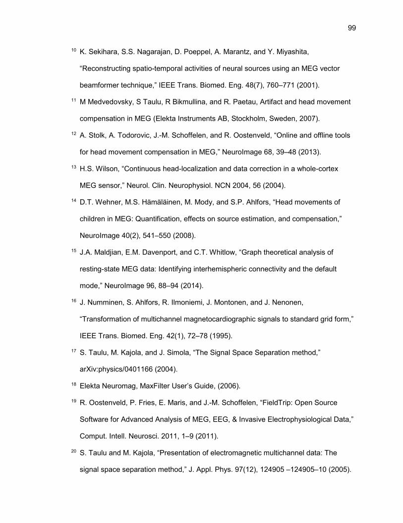
99

10 K. Sekihara, S.S. Nagarajan, D. Poeppel, A. Marantz, and Y. Miyashita,

“Reconstructing spatio-temporal activities of neural sources using an MEG vector

beamformer technique,” IEEE Trans. Biomed. Eng. 48(7), 760–771 (2001).

11 M Medvedovsky, S Taulu, R Bikmullina, and R. Paetau, Artifact and head movement

compensation in MEG (Elekta Instruments AB, Stockholm, Sweden, 2007).

12 A. Stolk, A. Todorovic, J.-M. Schoffelen, and R. Oostenveld, “Online and offline tools

for head movement compensation in MEG,” NeuroImage 68, 39–48 (2013).

13 H.S. Wilson, “Continuous head-localization and data correction in a whole-cortex

MEG sensor,” Neurol. Clin. Neurophysiol. NCN 2004, 56 (2004).

14 D.T. Wehner, M.S. Hämäläinen, M. Mody, and S.P. Ahlfors, “Head movements of

children in MEG: Quantification, effects on source estimation, and compensation,”

NeuroImage 40(2), 541–550 (2008).

15 J.A. Maldjian, E.M. Davenport, and C.T. Whitlow, “Graph theoretical analysis of

resting-state MEG data: Identifying interhemispheric connectivity and the default

mode,” NeuroImage 96, 88–94 (2014).

16 J. Numminen, S. Ahlfors, R. Ilmoniemi, J. Montonen, and J. Nenonen,

“Transformation of multichannel magnetocardiographic signals to standard grid form,”

IEEE Trans. Biomed. Eng. 42(1), 72–78 (1995).

17 S. Taulu, M. Kajola, and J. Simola, “The Signal Space Separation method,”

arXiv:physics/0401166 (2004).

18 Elekta Neuromag, MaxFilter User’s Guide, (2006).

19 R. Oostenveld, P. Fries, E. Maris, and J.-M. Schoffelen, “FieldTrip: Open Source

Software for Advanced Analysis of MEG, EEG, & Invasive Electrophysiological Data,”

Comput. Intell. Neurosci. 2011, 1–9 (2011).

20 S. Taulu and M. Kajola, “Presentation of electromagnetic multichannel data: The

signal space separation method,” J. Appl. Phys. 97(12), 124905 –124905–10 (2005).

100

21 G. Jansen, “Transformation properties of spheroidal multipole moments and

potentials,” J. Phys. Math. Gen. 33(7), 1375 (2000).

22 H. Wilson, Motion compensation in biomagnetic measurement, 7062391, 2006.

23 S. Taulu and J. Simola, “Spatiotemporal signal space separation method for rejecting

nearby interference in MEG measurements,” Phys. Med. Biol. 51(7), 1759–1768

(2006).

24 K.J. Friston et al., “Analysis of fMRI Time-Series Revisited,” NeuroImage 2(1), 45–53

(1995).

25 K.J. Worsley and K.J. Friston, “Analysis of fMRI Time-Series Revisited—Again,”

NeuroImage 2(3), 173–181 (1995).

26 F.E. Turkheimer et al., “Statistical Modeling of Positron Emission Tomography Images

in Wavelet Space,” J. Cereb. Blood Flow Metab. 20(11), 1610–1618 (2000).

27 S.J. Kiebel and Holmes, A. P., “The general linear model,” Hum. Brain Funct. Acad.

Press 2003(2nd edition), 1–58 (2003).

28 K. Uutela, S. Taulu, and M. Hämäläinen, “Detecting and Correcting for Head

Movements in Neuromagnetic Measurements,” NeuroImage 14(6), 1424–1431

(2001).

29 S. Brigadoi et al., “Motion artifacts in functional near-infrared spectroscopy: A

comparison of motion correction techniques applied to real cognitive data,”

NeuroImage (n.d.).

30 F.C. Robertson, T.S. Douglas, and E.M. Meintjes, “Motion Artifact Removal for

Functional Near Infrared Spectroscopy: A Comparison of Methods,” IEEE Trans.

Biomed. Eng. 57(6), 1377–1387 (2010).

31 F. Scholkmann, S. Spichtig, T. Muehlemann, and M. Wolf, “How to detect and reduce

movement artifacts in near-infrared imaging using moving standard deviation and

spline interpolation,” Physiol. Meas. 31(5), 649 (2010).

101

32 S. Liu, Q. He, R.X. Gao, and P. Freedson, “Empirical mode decomposition applied to

tissue artifact removal from respiratory signal,” in 30th Annu. Int. Conf. IEEE Eng.

Med. Biol. Soc. 2008 EMBS 2008(2008), pp. 3624–3627.

33 R.J. Cooper et al., “A Systematic Comparison of Motion Artifact Correction

Techniques for Functional Near-Infrared Spectroscopy,” Front. Neurosci. 6, (2012).

34 M.J. Brookes et al., “Beamformer reconstruction of correlated sources using a

modified source model,” NeuroImage 34(4), 1454–1465 (2007).

35 A. Matheny and D.B. Goldgof, “The use of three- and four-dimensional surface

harmonics for rigid and nonrigid shape recovery and representation,” IEEE Trans.

Pattern Anal. Mach. Intell. 17(10), 967–981 (1995).

36 J.P. Bardhan and M.G. Knepley, “Computational science and re-discovery: open-

source implementation of ellipsoidal harmonics for problems in potential theory,”

Comput. Sci. Discov. 5(1), 014006 (2012).

37 M. Danos and L.C. Maximon, “Multipole Matrix Elements of the Translation Operator,”

J. Math. Phys. 6(5), 766–778 (1965).

38 C. Lessig, T. de Witt, and E. Fiume, “Efficient and accurate rotation of finite spherical

harmonics expansions,” J. Comput. Phys. 231(2), 243–250 (2012).

39 Spheroid, Wikipedia Free Encycl. (2014).

40 Oblate spheroidal coordinates, Wikipedia Free Encycl. (2014).

41 Prolate spheroidal coordinates, Wikipedia Free Encycl. (2014).

42 Latitude, Wikipedia Free Encycl. (2015).

43 C. Jekeli, “The exact transformation between ellipsoidal and spherical harmonic

expansions.,” Manuscripta geodaetica 13(2), 106–113 (1988).

44 J. Sebera, J. Bouman, and W. Bosch, “On computing ellipsoidal harmonics using

Jekeli’s renormalization,” J. Geod. 86(9), 713–726 (2012).

102

45 F.J. Lowes and D.E. Winch, “Orthogonality of harmonic potentials and fields in

spheroidal and ellipsoidal coordinates: application to geomagnetism and geodesy,”

Geophys. J. Int. 191(2), 491–507 (2012).

46 L.-W. Li, M.-S. Leong, T.-S. Yeo, P.-S. Kooi, and K.-Y. Tan, “Computations of

spheroidal harmonics with complex arguments: A review with an algorithm,” Phys.

Rev. E 58(5), 6792–6806 (1998).

47 A.A. White, A. Staniforth, and N. Wood, “Spheroidal coordinate systems for modelling

global atmospheres,” Q. J. R. Meteorol. Soc. 134(630), 261–270 (2008).

48 G. Romain and B. Jean-Pierre, “Ellipsoidal Harmonic expansions of the gravitational

potential: Theory and application,” Celest. Mech. Dyn. Astron. 79(4), 235–275 (2001).

49 B. Hofmann-Wellenhof and H. Moritz, Physical Geodesy (Springer Science &

Business Media, 2006).

50 J.A. Tropp and A.C. Gilbert, “Signal Recovery From Random Measurements Via

Orthogonal Matching Pursuit,” IEEE Trans. Inf. Theory 53(12), 4655–4666 (2007).

51 J. Nenonen et al., “Validation of head movement correction and spatiotemporal signal

space separation in magnetoencephalography,” Clin. Neurophysiol. 123(11), 2180–

2191 (2012).

52 M. Medvedovsky, S. Taulu, R. Bikmullina, and R. Paetau, “Artifact and head

movement compensation in MEG,” Neurol. Neurophysiol. Neurosci. 4 (2007).

53 M.J. Mohlenkamp, “A fast transform for spherical harmonics,” J. Fourier Anal. Appl.

5(2-3), 159–184 (1999).

103

VII. APPENDIX I

Laplace’s equation in the oblate spheroidal coordinate system can be separated into

three ordinary differential equations, two of which are identical to the spherical

coordinate case and are not included here for brevity (Physical Geodesy, page 38) 49.

The third equation is corresponding to the radial equation in the spherical case. This

equation in the oblate coordinate system is derived below in the current notation 49:

�/ + '/�l�� �� + /�l� �� − k� � + 0� − '/=/�/ + '/m l �� = � Eq. ( 1 )

Substituting 3 � '9 with � converts Eq. ( 1 ) to the following equation:

;0 − �/@l�� �� − /�l� �� + k� � + 0� − =/0 − �/m l �� = � Eq. ( 2 )

There are two possible solutions to the equation above:

l �� = _�= N3 �'O <4� ��= N3 �'O Eq. ( 3 )

Eq. ( 1 ) can be converted to the prolate coordinate system by multiplying the variable '

with 0/3 :

�/ − '/�l�� �� + /�l� �� − k� � + 0� + '/=/�/ − '/m l �� = � Eq. ( 4 )

104

Substituting � '9 with � converts Eq. ( 4 ) to the following equation:

−0� �;0 − �/@l�� �� − /�l� �� + k� � + 0� − =/0 − �/m l ��� = � Eq. ( 5 )

Eq. ( 5 ) is identical to Eq. ( 2 ) and has the same solution but with a different argument:

l �� = _�= N�'O <4� ��= N�'O Eq. ( 6 )

105

VIII. CURRICULUM VITAE

Inna V. McGowin, M.S., Ph.D.

mcgowii@gmail.com

EDUCATION:

Bachelor of Science

Rostov-on-Don Pedagogical University (1994-2001)

Rostov-on-Don, Russia

major: Physics

minor: Computer Science

Master of Science

East Carolina University (2007-2009)

Greenville, NC USA

major: Physics (CAMPEP)

concentration: Medical Physics

Doctor of Philosophy

Wake Forest University (2010-2015)

Winston-Salem, NC USA

major: Physics

concentration: Medical Physics

SPECIALTY CERTIFICATION:

American Board of Radiology Diagnostic and Therapeutic Physics Part I, Passed ABR

Part I September 2009 (eligible for Part II)

PROFESSIONAL MEMBERSHIPS:

American Physical Society (APS) 2006-present

American Association of Physicists in Medicine (AAPM) 2007-present

106

American Clinical Magnetoencephalography 2013-present

Society (ACMEGS)

PROFESSIONAL INTERESTS:

Diagnostic and pre-surgical brain imaging with MRI, fMRI, MEG and EEG; relation

between brain tumor radiation dose (and isodoses) and post-irradiation functional brain

changes; non-invasive brain functional mapping (such as motor, somato-sensory and

language cortices); MEG language lateralization in patients and healthy subjects;

statistical analysis in multimodal imaging approach to a detection and treatment of a

disease (such as brain tumor or epilepsy focus); post-irradiation dose measurement and

calculation and their correlations with the treatment outcomes.

CLINICAL, RESEARCH AND COMPUTATIONAL SKILLS:

IMRT QA preparation in Pinnacle and testing on Elekta and Varian, Table Imaging QA,

blocks and physical IMRT compensators manufacturing and testing.

Skilled to evaluate my and that of others work and find possible errors or flaws, being

able to work without close supervision and take initiative, being able to work on a

problem without “a right answer”.

Have extensive teaching experience in Physics and Computer Skills.

Proficient in using Windows, Linux, Matlab, MOSAIQ, Magnetoencephalography

Scanner, Curry, BrainSuite, Microsoft Office and more.

PUBLICATIONS:

1. Ding X, Olsen J, Best R, Bennett M, McGowin I, Dorand J, Link K, Bourland JD. High

resolution polymer gel dosimetry for small beam irradiation using a 7T micro-MRI

scanner. IC3DDose: The 6th International Conference on 3D Radiation Dosimetry.

Journal of Physics: Conference Series 250 (2010) 012094 (Proceedings)

2. Inna V. McGowin, Greg E. Alberto, Justin B. Rawley, J. Daniel Bourland, Dwayne W.

Godwin: Evaluation and quantitative comparison of two head motion correction methods,

Single Space Separation and General Linear Modelling, in Magnetoencephalography (in

revision for resubmission, 2015)

107

ABSTRACTS AND PRESENTATIONS:

1. Ding X, Bourland J, Dolesh W, Best R, Mcgowin I, Liu J, Small field output factor

measurement using MAGIC gel dosimeter in 3T MRI. Med. Phys. 39: 3725 (2012)

(abstract)

2. Ding X, Bourland J, Dolesh W, Best R, Mcgowin I, Liu J, Small field output factor

measurement using MAGIC gel dosimeter in 3T MRI. Med. Phys. 39: 3725 (2012)

(abstract)

3. McGowin I, Bourland J, Peiffer A, Simpson S, Rawley J, Godwin D.

Magnetoencephalography (MEG): quantitative comparison of oscillations and

synchronization differences/similarities in post-surgery/pre-irradiation patients and

control subjects. Med Phys 40:146, 2013 (abstract)

4. McGowin I, Bourland J, Peiffer A, Simpson S, Rawley J, Godwin D.

Magnetoencephalography (MEG): quantitative comparison of oscillations and

synchronization differences/similarities in post-surgery/pre-irradiation patients and

control subjects. 55th Annual Meeting of the AAPM, Indianapolis, IN, August, 2013

(poster presentation)

REFERENCES

J. Daniel Bourland, PhD, FAAPM

Professor with Tenure

Department of Radiation Oncology, Physics and

Biomedical Engineering

Wake Forest School of Medicine and Wake Forest University

Radiation Oncology, Comprehensive Cancer Center

Brain Tumor Center of Excellence

Medical Center Boulevard, Winston-Salem, NC 27157

(office) 336-713-6503

bourland@wakehealth.edu

Dwayne W. Godwin, PhD

Professor and Dean

108

Graduate School of Arts and Science

Graduate Education

Biomedical Sciences Programs

Neurobiology & Anatomy

Institute for Regenerative Medicine

Neurology, Physiology & Pharmacology

Wake Forest School of Medicine and Wake Forest University

Medical Center Boulevard, Winston-Salem, NC 27157

(office) 336-716-4303

dgodwin@wakehealth.edu

V. Paul Pauca, PhD

Associate Professor

Department of Computer Science

Wake Forest University

Manchester Hall, 235

Winston-Salem, NC 27109

(office) 336-758-5454

paucavp@wfu.edu

Eric K. Chapman, BS

Instructional Resources Manager

Department of Physics

Wake Forest University

100 Olin Physical Laboratory

Winston-Salem, NC 27109

(office) 336-758-5532

chapmaek@wfu.edu