engineering economics - civil teamcivil-team.weebly.com/uploads/2/5/8/2/25829430/d... · what is...
TRANSCRIPT

ENGINEERING ECONOMICSECONOMICS

WHAT IS ECONOMICS ?
The study of how limited resources is used to satisfy unlimited human satisfy unlimited human wants

WHAT IS ECONOMICS ?عرف ا�قتصاد الھندسي بأنه فرع من ا�قتصاد الذي يطبق
في المشاريع الھندسية

WHAT IS Engineering economics?
,
previously known as engineering economy, is a subset of economy, is a subset of economics for application to engineering projects.

WHAT IS ECONOMICS ?
. Engineers seek solutions to problems, and the economic viability of each potential viability of each potential solution is normally considered along with the technical aspects

Introduction to Engineering Economy
التقييم المنھجي لتكاليف و منافع المشاريع التقنية •المقترحة
تستخدم مبادئ و مناھج ا�قتصاد الھندسي في تحليل •
٦
تستخدم مبادئ و مناھج ا�قتصاد الھندسي في تحليل •بدائل ا�ستخدامات البديلة للموارد المالية المتعلقة
با5صول الفيزيائية و الجوانب العم1نية للمؤسسات الھندسية

Introduction to Engineering Economy
• The systematic evaluation of the costs and benefits of proposed technical projects
• The principles and methodology of engineering economy are • The principles and methodology of engineering economy are utilized to analyze alternative uses of financial resources, particularly in relation to the physical assets and the operation of an organization.
٧

Decision Making and Problem Solving
Simple Problems
Intermediate Problems (Principle subject of this course!!!)
Complex Problems
٨
Decision Making and Problem Solving
Simple Problems• Can be analyzed in one’s head without extensive analysis
– Do I buy a semester parking pass or use parking meters?– Should I fix my car?
Intermediate Problems (Principle subject of this course!!!)• They are sufficiently important to justify serious thought and action• They can’t be worked in one’s head; must be organized • The economic aspects are significant component in the analysis leading to a
decision
Complex Problems• Represent a mixture of economic, political, and humanistic elements
– Selection of a president in USA– Building a nuclear power plant
٩

THE ROLE OF ENGINEERING ECONOMIC ANALYSIS
• 1. The problem is important enough to justify our giving it serious thought and effort.
• 2. The problem can't be worked in one's head-that is, a careful analysis requires that we organize the problem and all the various consequences, and this is just too much to be done all at once.

THE ROLE OF ENGINEERING ECONOMIC
ANALYSIS
• 3. The problem has economic aspects important in reaching a decision.important in reaching a decision.

Examples of Engineering Economic Analysis
• Engineering economic analysis focuses on costs, revenues, and benefits that occur at different times. For example, when a civil engineer "designs a road, a when a civil engineer "designs a road, a dam, or a building, the construction costs occur in the near future; the benefits to users begin only when construction is finished, but then the benefits continue for a long time.

Examples of Engineering Economic Analysis
ما ھي المشاريع الھندسية الجديرة با�ھتمام •ما ھي المشاريع الھندسية ذات ا5ولوية•ھل اختار المھندس المحرك المناسب• ھل اختار المھندس المحرك المناسب•ھل اختار المھندس السماكة و النوعية المناسبة لمادة •
العزلھل وازن بين بديلين احدھما مكلف و آمن و ا>خر اقل •
كلفة و اقل أمنا
Rational Decision Making
1. Recognize the problem– “I need a place to live this term.”
2. Define the Goal or Objective– “I’ll find a nice apartment that is not too expensive.”
3. Assemble Relevant Data
١٤
3. Assemble Relevant Data– “I need information on rent, utilities, apartment age, parking, driving time
to UF, driving time to shopping, the neighborhood, other amenities provided (swimming, table tennis, etc.).”
4. Identify Feasible Alternatives– “I’ll use the Yellow Pages, information from friends, apartment finding
services, information from UF, the local newspaper, and my personal experience, to look for apartments.”

Rational Decision Making
5. Select Criterion to Determine the Best Alternative– “Most important is rent plus utilities cost. I’m also very concerned about driving
time to UF, and the kind of neighborhood the apartment is in.”
6. Construct the model– “I’ll make a spreadsheet. The rows will be the apartment choices, the columns
the evaluation criteria. Then I’ll try to fill in the interactions between the apartments and the criteria.”
– This includes determining cash flows for engineering economic analysis!!!
١٥
– This includes determining cash flows for engineering economic analysis!!!
7. Predict Outcomes of Each Alternative– “I’ll fill in the estimated costs for the spreadsheet and rate the amenities, driving
time, etc.”
8. Choose the Best Alternative– “Apartment C looks cheapest, but I don`t like the neighborhood. If I pay $50
more per month for Apartment B I get a nicer neighborhood, and a 15-minute drive to UF. Maybe I’ll choose Apartment B.”
Rational Decision Making
9. Audit the Results
– “Did I make a good choice”
١٦
– “After living in Apartment B for six months, I am very happy with my choice!”
– But this certainly isn’t the case every time!!

Rational Decision Making
التعرف على المشكلة١.
تحديد الھدف٢.
تجميع البيانات ذات الصلة٣.
تحديد البدائل الممكنة٤.
١٧
تحديد البدائل الممكنة٤.
اختيارالمعايير المناسبة لتحديد افضل البدائل٥.
بناء النموذج٦.
توقع النتائج المتعلقة بكل من البدائل٧.
اختيار البديل ا5فضل٨.
مراجعة النتائج٩.

PRINCIPLES OF ENGINEERING ECONOMY
1. Develop the Alternatives;
2. Focus on the Differences;
3. Use a Consistent Viewpoint;3. Use a Consistent Viewpoint;
4. Use a Common Unit of Measure;
5. Consider All Relevant Criteria;
6. Make Uncertainty Explicit;
7. Revisit Your Decisions

DEVELOP THE ALTERNATIVES
The final choice (decision) is among alternatives. The alternatives need to be identified and then defined for subsequent analysis.subsequent analysis.

Examples of Engineering Economic Analysis
• Engineering economic analysis is used to answer many different questions. · Which engineering projects are worthwhile? Has the mining or petroleum engineer shown that the petroleum engineer shown that the mineral or oil deposit is worth developing?
• · Which engineering projects should have a higher priority? Has the industrial engineer shown which factory improvement projects should be funded

FOCUS ON THE DIFFERENCES
يجب ا�ھتمام با�خت1فات المستقبلية بين البدائل المقارنة

USE A CONSISTENT VIEWPOINT
The prospective outcomes of the alternatives, economic and other, should be consistently developed from a defined viewpoint (perspective).viewpoint (perspective).

CONSIDER ALL RELEVANT CRITERIA
Selection of a preferred alternative (decision making) requires the use of a criterion (or several criteria). The decision process should consider the decision process should consider the outcomes enumerated in the monetary unit and those expressed in some other unit of measurement or made explicit in a descriptive manner.

USE A COMMON UNIT OF MEASURE
Using a common unit of measurement to enumerate as many of the prospective outcomes as possible will make easier the analysis and comparison of the analysis and comparison of alternatives.

MAKE UNCERTAINTY EXPLICIT
Uncertainty is inherent in projecting (or estimating) the future outcomes of the alternatives and should be recognized in their analysis and comparison.their analysis and comparison.

MAKE UNCERTAINTY EXPLICIT
ماذا يحدث اذا زادت التكاليف •
ماذا يحدث اذا انخفضت التكاليف•
ماذا يحدث اذا انخفضت ا�يرادات• ماذا يحدث اذا انخفضت ا�يرادات•
ماذا يحدث اذا انخفضت ا�يرادات و زادت التكاليف•

REVISIT YOUR DECISIONSImproved decision making results from an adaptive process; to the extent practicable, the initial projected outcomes of the selected alternative should be subsequently compared with actual subsequently compared with actual results achieved.

Time Value of Money
• The following are reasons why $1000 today is
• “worth” more than $1000 one year from today:
• 1. Inflation
• 2. Risk
• 3. Cost of money

INTEREST
The fee that a borrower pays to a lender for the use of his or her money.money.
INTEREST RATE
The percentage of money being borrowed that is paid to the lender on some time basis.

Concept of Interest
If you won the lotto, would you rather get $1 Million now or $50,000 for 25 years?
What about automobile and home financing? What type of financing makes more economic sense?
Interest: Money paid for the use of borrowed money.
• Put simply, interest is the rental charge for using an asset over some period of time and then, returning the asset in the same conditions as we received it.
→ In project financing, the asset is usually money
Why Interest exist?
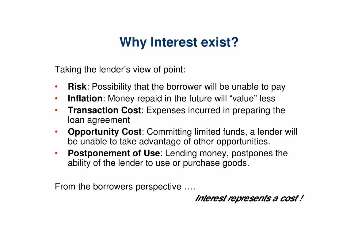
Taking the lender’s view of point:
• Risk: Possibility that the borrower will be unable to pay
• Inflation: Money repaid in the future will “value” less
• Transaction Cost: Expenses incurred in preparing the loan agreementloan agreement
• Opportunity Cost: Committing limited funds, a lender will be unable to take advantage of other opportunities.
• Postponement of Use: Lending money, postpones the ability of the lender to use or purchase goods.
From the borrowers perspective ….
Interest represents a cost !

Simple Interest
Simple Interest is also known as the Nominal Rate of Interest
� Annualized percentage of the amount borrowed (principal) which is paid for the use of the money for some period of time.
Suppose you invested $1,000 for one year at 6% simple rate; at the end of one year the investment would yield:
$1,000 + $1,000(0.06) = $1,060
This means that each year interest gives $60
How much will you earn (including principal) after 3 years?
$1,000 + $1,000(0.06) + $1,000(0.06) + $1,000(0.06) = $1,180
Note that for each year, the interest earned is only calculated over $1,000.Does this mean that you could draw the $60 earned at the end of each year?

HOW INTEREST RATE IS DETERMINED
HOW INTEREST RATE IS DETERMINEDInterest
RateMoney Supply
MS1 MS2MS3
i3
Quantity of Money
ie
Money Demandi2

SIMPLE INTEREST• The total interest earned or charged is linearly
proportional to the initial amount of the loan (principal), the interest rate and the number of interest periods for which the principal is committed.committed.
• When applied, total interest “I” may be found by I = ( P ) ( N ) ( i ), where
– P = principal amount lent or borrowed
– N = number of interest periods ( e.g., years )
– i = interest rate per interest period

Terms
In most situations, the percentage is not paid at the end of the period, where the interestearned is instead added to the original amount (principal). In this case, interest earned fromprevious periods is part of the basis for calculating the new interest payment.
This “adding up” defines the concept of Compounded Interest
Now assume you invested $1,000 for two years at 6% compounded annually;
At the end of one year the investment would yield:
$1,000 + $1,000 ( 0.06 ) = $1,060 or $1,000 ( 1 + 0.06 )
Since interest is compounded annually, at the end of the second year the investment would be worth:
[ $1,000 ( 1 + 0.06 ) ] + [ $1,000 ( 1 + 0.06 ) ( 0.06 ) ] = $1,124Principal and Interest for First Year Interest for Second Year
Factorizing:
$1,000 ( 1 + 0.06 ) ( 1 + 0.06 ) = $1,000 ( 1 + 0.06 )2 = $1,124
How much this investment would yield at the end of year 3?

ECONOMIC EQUIVALENCE• Established when we are indifferent between a
future payment, or a series of future payments, and a present sum of money .
• Considers the comparison of alternative options, or proposals, by reducing them to an equivalent basis, depending on:equivalent basis, depending on:
– interest rate;
– amounts of money involved;
– timing of the affected monetary receipts and/or expenditures;
– manner in which the interest , or profit on invested capital is paid and the initial capital is recovered.

ECONOMIC EQUIVALENCE FOR FOUR REPAYMENT PLANS OF AN $8,000 LOAN
• Plan #1: $2,000 of loan principal plus 10% of BOY principal paid at the end of year; interest paid at the end of each year is reduced by $200 (i.e., 10% of remaining principal)
Year Amount Owed Interest Accrued Total Principal Total end at beginning for Year Money Payment of Year at beginning for Year Money Payment of Year of Year owed at Payment ( BOY ) end of
Year
1 $8,000 $800 $8,800 $2,000 $2,800
2 $6,000 $600 $6,600 $2,000 $2,600
3 $4,000 $400 $4,400 $2,000 $2,400
4 $2,000 $200 $2,200 $2,000 $2,200
Total interest paid ($2,000) is 10% of total dollar-years ($20,000)

• Plan #2: $0 of loan principal paid until end of fourth year; $800 interest paid at the end of each year
Year Amount Owed Interest Accrued Total Principal Total end at beginning for Year Money Payment of Year of Year owed at Payment of Year owed at Payment ( BOY ) end of
Year
1 $8,000 $800 $8,800 $0 $800
2 $8,000 $800 $8,800 $0 $800
3 $8,000 $800 $8,800 $0 $800
4 $8,000 $800 $8,800 $8,000 $8,800
Total interest paid ($3,200) is 10% of total dollar-years ($32,000)

ECONOMIC EQUIVALENCE FOR FOUR REPAYMENT PLANS OF AN $8,000 LOAN
• Plan #3: $2,524 paid at the end of each year; interest paid at the end of each year is 10% of amount owed at the beginning of the year.
Year Amount Owed Interest Accrued Total Principal Total end at beginning for Year Money Payment of Year of Year owed at Payment ( BOY ) end of
Year
1 $8,000 $800 $8,800 $1,724 $2,524
2 $6,276 $628 $6,904 $1,896 $2,524
3 $4,380 $438 $4,818 $2,086 $2,524
4 $2,294 $230 $2,524 $2,294 $2,524
Total interest paid ($2,096) is 10% of total dollar-years ($20,950)

ECONOMIC EQUIVALENCE FOR FOUR REPAYMENT PLANS OF AN $8,000 LOAN
• Plan #4: No interest and no principal paid for first three years. At the end of the fourth year, the original principal plus accumulated (compounded) interest is paid.
Year Amount Owed Interest Accrued Total Principal Total end at beginning for Year Money Payment of Year at beginning for Year Money Payment of Year of Year owed at Payment ( BOY ) end of
Year
1 $8,000 $800 $8,800 $0 $0
2 $8,800 $880 $9,680 $0 $0
3 $9,680 $968 $10,648 $0 $0
4 $10,648 $1,065 $11,713 $8,000 $11,713
Total interest paid ($3,713) is 10% of total dollar-years ($37,128)

CASH FLOW DIAGRAMS / TABLE NOTATION
CASH FLOW DIAGRAMS / TABLE NOTATION
i = effective interest rate per interest period
N = number of compounding periods (e.g., years)
P = present sum of money; the equivalent value of one or more cash flows at the present time reference point
F = future sum of money; the equivalent value of one or
i = effective interest rate per interest period
N = number of compounding periods (e.g., years)
P = present sum of money; the equivalent value of one or more cash flows at the present time reference point
F = future sum of money; the equivalent value of one or more cash flows at a future time reference point
A = end-of-period cash flows (or equivalent end-of-period values ) in a uniform series continuing for a specified number of periods, starting at the end of the first period and continuing through the last period
G = uniform gradient amounts -- used if cash flows increase by a constant amount in each period
more cash flows at a future time reference point
A = end-of-period cash flows (or equivalent end-of-period values ) in a uniform series continuing for a specified number of periods, starting at the end of the first period and continuing through the last period
G = uniform gradient amounts -- used if cash flows increase by a constant amount in each period
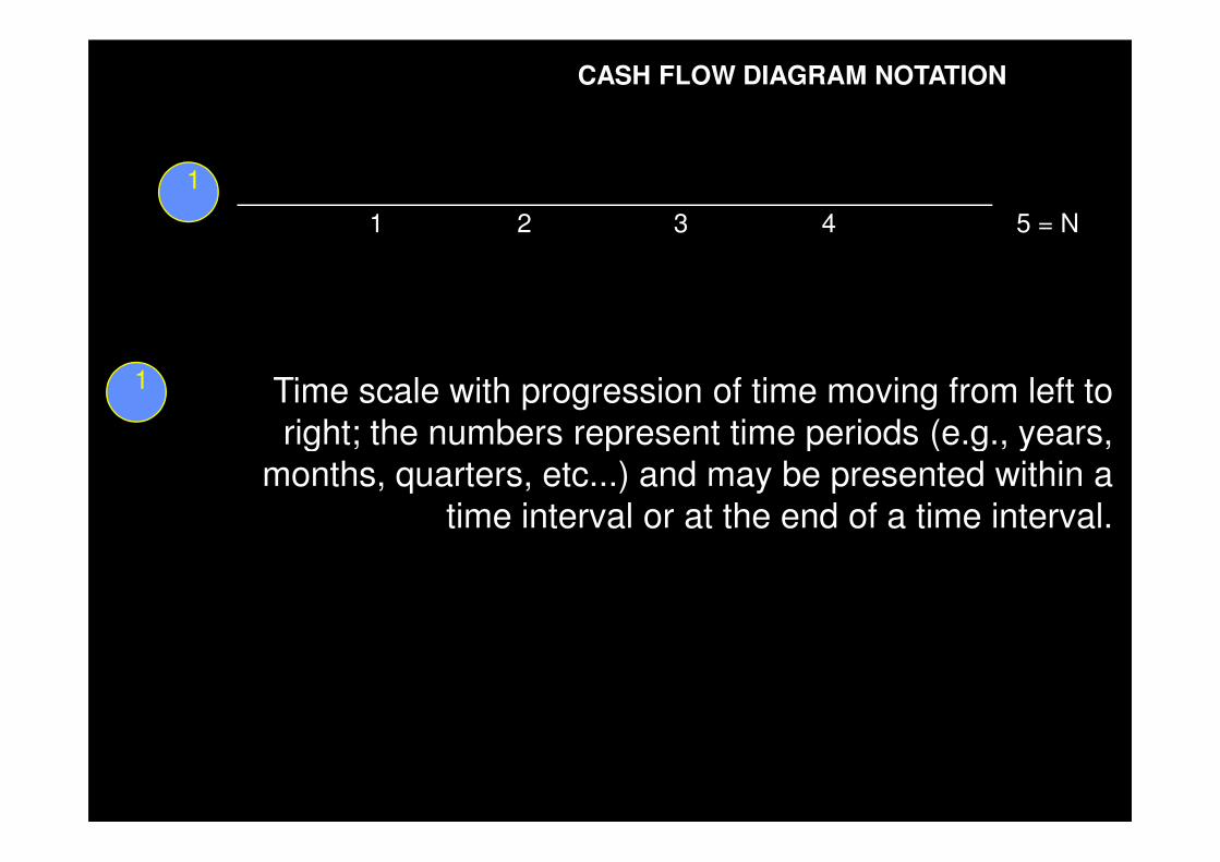
CASH FLOW DIAGRAM NOTATION
1 2 3 4 5 = N
1
1 Time scale with progression of time moving from left to right; the numbers represent time periods (e.g., years, right; the numbers represent time periods (e.g., years,
months, quarters, etc...) and may be presented within a time interval or at the end of a time interval.

CASH FLOW DIAGRAM NOTATION
1 2 3 4 5 = N
1
1 Time scale with progression of time moving from left to right; the numbers represent time periods (e.g., years,
P =$8,0002
right; the numbers represent time periods (e.g., years, months, quarters, etc...) and may be presented within a
time interval or at the end of a time interval.
2Present expense (cash outflow) of $8,000 for lender.

CASH FLOW DIAGRAM NOTATION
1 2 3 4 5 = N
1
1 Time scale with progression of time moving from left to right; the numbers represent time periods (e.g., years,
P =$8,0002
A = $2,524 3
right; the numbers represent time periods (e.g., years, months, quarters, etc...) and may be presented within a
time interval or at the end of a time interval.
2Present expense (cash outflow) of $8,000 for lender.
3 Annual income (cash inflow) of $2,524 for lender.

CASH FLOW DIAGRAM NOTATION
1 2 3 4 5 = N
1
1 Time scale with progression of time moving from left to right; the numbers represent time periods (e.g., years,
P =$8,0002
A = $2,524 3
i = 10% per year4
right; the numbers represent time periods (e.g., years, months, quarters, etc...) and may be presented within a
time interval or at the end of a time interval.
2Present expense (cash outflow) of $8,000 for lender.
3 Annual income (cash inflow) of $2,524 for lender.
4Interest rate of loan.
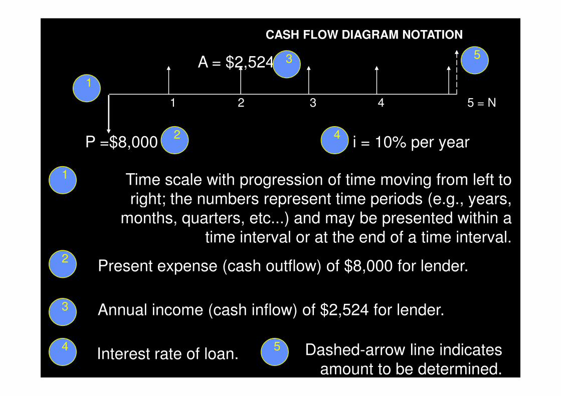
CASH FLOW DIAGRAM NOTATION
1 2 3 4 5 = N
1
1 Time scale with progression of time moving from left to right; the numbers represent time periods (e.g., years,
P =$8,0002
A = $2,524 3
i = 10% per year4
5
right; the numbers represent time periods (e.g., years, months, quarters, etc...) and may be presented within a
time interval or at the end of a time interval.
2Present expense (cash outflow) of $8,000 for lender.
3 Annual income (cash inflow) of $2,524 for lender.
4Interest rate of loan.
5 Dashed-arrow line indicatesamount to be determined.

Single Payment Factors: (F/P, i ,n)
Find F
P is given (i and n are also given)
1 2 n
47
Recall that F = P(1 + i)n
Given P, to find F, the conversion factor is (1+i)n
F = P (F/P, i ,n) where (F/P, i ,n) = (1+ i)n
(F/P, i, n) is tabulated for different i and nFV(i%,n,,P) in Excel

If $1,000 were deposited in a savings a/c, what would be the ac/ balance in two years if the bank paid 4% interest per year compounded annually?
Single Payment Factors: (F/P, i ,n)
48
Solution: P = $1,000, n = 2, i = 4%, F = ?
F = P(1+i)n = $1,000 (1 + 0.04)2 = $1,081.60, or
the factor (F/P, 4%, 2) is 1.0818
F = P (F/P, 4%, 2) = $1,000 (1.0816) = 1,081.80

Single Payment Factor: (P/F, i ,n)
Find P (i and n are also given)
F given
F = P(1 + i)n or P = F /(1 + i)n
49
F = P(1 + i)n or P = F /(1 + i)n
So 1/(1+i)n is the P/F conversion factor
P = F (P/F, i ,n)
where (P/F, i ,n) = 1/(1+ i)n
(P/F, i, n) is tabulated for different i PV(i%,n,,F) in Excel

If you wished to have $1,082 in a savings
account at the end of two years and 4% interest
was paid annually, how much should you put
Single Payment Factor: (P/F, i ,n
50
was paid annually, how much should you put
into the savings account now?
Solution: P = ?, n = 2, i = 4%, F = $1,082
P = F/(1+i)n = $1,082/(1 + 0.04)2 = $1,000.37, or
P = F (P/F, 4%, 2) = $1,000.37

Find the future worth of this cash flow series 10 Y at
0 1 2 3 4 5 6 7
$600
$300 $400
(+)
(-)
51
Find the future worth of this cash flow series 10 Y at an interest rate of 5% per year.
Solution: F10 = - 600 (F/P,5%,10) – 300 (F/P,5%,8) –400 (F/P,5%,5) = -1931.08

Find the equivalent single payment of this cash flow
13 14 15 27
$300
$700
52
Find the equivalent single payment of this cash flow series 15 Y at an interest rate of 5% per year.
Solution: F15 = -300(F/P,5%,2) +700(P/F,5%,12) = 59.04

Equal Payment Series
A
0 1 2 3 4 5 N-1 N
FF
P

Uniform Series Present Worth Factor (P/A, i , n)
P = ?
54
�Objective: Find P, given A
2 … n-1 n1
A AAA
0

A uniform series of payments or receipts represents:
A collection of end-of-period cash payments or receipts arranged in a uniform series and continuing for n periods. Such a series is equivalent to P or F at interest rate i, given the constant cash payment (or receipt) designated as A (based on the term “annuity”, a regular payment).
Consider a 4-yr period:Consider a 4-yr period:
A A A A| | | |
F = 0..1..2..3..4 + 0..1..2..3..4 + 0..1..2..3..4 + 0..1..2..3..4| | | |A| | | A(1+i)1
| | A(1+i)2
| A(1+i)3

Uniform series (contin.)
F = A(1+i)3 + A(1+i)2 + A(1+i)1 + A Now, multiply by (1+i)
(1+i) F = A(1+i)4 + A(1+i)3 + A(1+i)2 + A(1+i) - F = A(1+i)3 + A(1+i)2 + A(1+i)1 + A Solve for the difference
i F = A(1+i)4 - A
= A[(1+i)4 - 1] Thus, F = A[(1+i)4 - 1] / i = A[(1+i)4 - 1] Thus, F = A[(1+i)4 - 1] / i
In general,
\ uniform series compound-amount factor
( )
−+=
i
iAF
n11

Uniform series (contin.)
If we turn this around and solve for A, we obtain:
\ uniform series sinking-fund factor
( )
−+=
11n
i
iFA
sinking-fund factor
Example: Set up a uniform-payment investment (college fund) with the goal of having $80,000 after 20 years, invested at 6% compounded annually. What is the required annual payment?
A = $80,000(.06)/[1.0620 –1] = $80,000(.06/2.207135) = $2174.77OR
A = F (A/F, 6%, 20) = $80,000(.0272) = $2176( ~ $182/mo.)

Uniform series (contin.)
If we take the uniform-series compounding equation and replace F with the single-payment compounding expression, we obtain:
uniform series ( )
( )
−+=+
i
iAiP
nn 11
1
present-worth factor
/
This expression is used to calculate the present worth, giventhe regular annuity payment.
i
( )
( )
+
−+=
n
n
ii
iAP
1
11

Example:
Our consulting firm would like to purchase a used testing machine from an independent testing/inspection lab, and we make two offers: 1) a lump-sum of $40,000 or 2) monthly payments of $1200 over 3 years at a 6% annual interest rate. Which option do you think the testing lab would prefer, assuming it has to replace the sold machine?
P = $1200 [P/A, 0.5%, 36] = $1200(32.871) = $39,445Ploan = $1200 [P/A, 0.5%, 36] = $1200(32.871) = $39,445
The lab would prefer the $40000 payment now, because it is greater than the present worth of the proposed loan terms.
Note: Floan = $1200[F/A, 0.5%, 36] = $1200(39.336) = $47,203

Uniform series (contin.)
If we instead solve for A, we obtain:
\
( )
( )
−+
+=
11
1n
n
i
iiPA
\ uniform series capital-recovery factor
This expression is used to calculate the regular annuity payment, given the present worth.

Standard Factor Notation
To Find Given Factor Equation
P F (P/F, i, n) P = F*(P/F, i, n)
F P (F/P, i, n) F = P*(F/P, i, n)
P A (P/A, i, n) P = A*(P/A, i, n)
A P (A/P, i, n) A = P*(A/P, i, n)
61
A P (A/P, i, n) A = P*(A/P, i, n)
A F (A/F, i, n) A = F*(A/F, i, n)
F A (F/A, i, n) F = A*(F/A, i, n)
Practice deriving these factor formulas directly using geometric sum identity
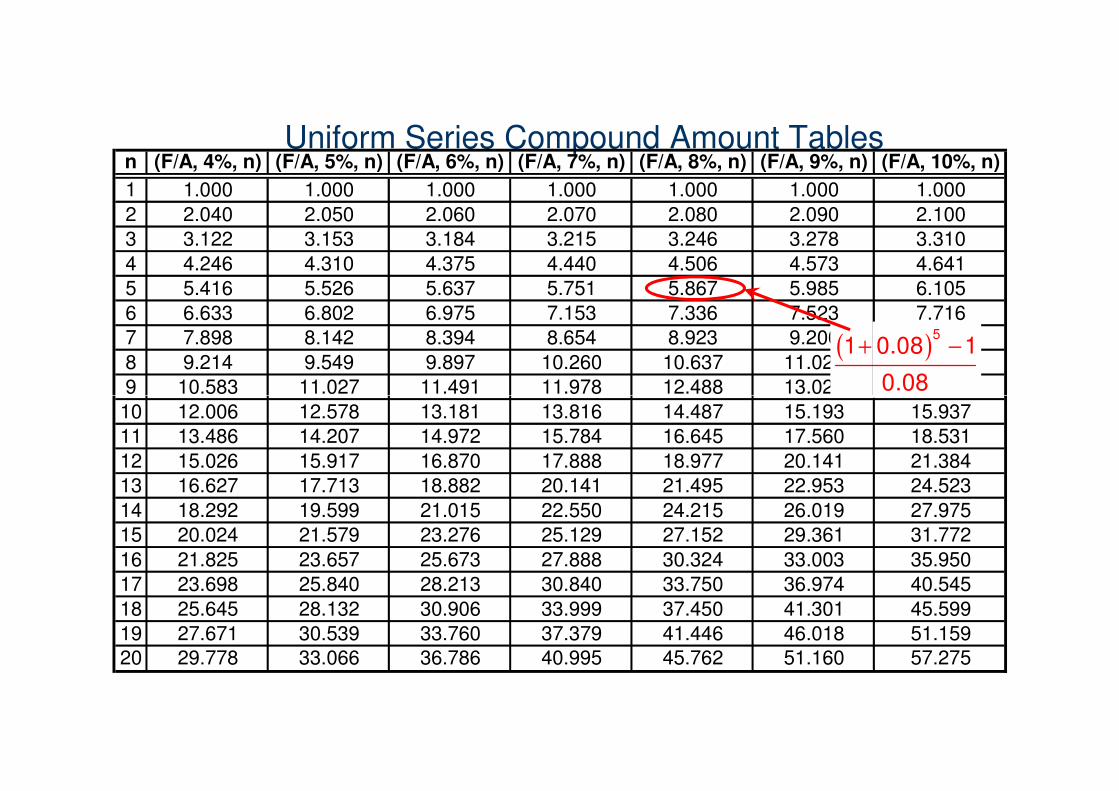
Uniform Series Compound Amount Tablesn (F/A, 4%, n) (F/A, 5%, n) (F/A, 6%, n) (F/A, 7%, n) (F/A, 8%, n) (F/A, 9%, n) (F/A, 10%, n)
1 1.000 1.000 1.000 1.000 1.000 1.000 1.000
2 2.040 2.050 2.060 2.070 2.080 2.090 2.100
3 3.122 3.153 3.184 3.215 3.246 3.278 3.310
4 4.246 4.310 4.375 4.440 4.506 4.573 4.641
5 5.416 5.526 5.637 5.751 5.867 5.985 6.105
6 6.633 6.802 6.975 7.153 7.336 7.523 7.716
7 7.898 8.142 8.394 8.654 8.923 9.200 9.487
8 9.214 9.549 9.897 10.260 10.637 11.028 11.436
9 10.583 11.027 11.491 11.978 12.488 13.021 13.579
( )+ −5
1 0.08 1
0.089 10.583 11.027 11.491 11.978 12.488 13.021 13.579
10 12.006 12.578 13.181 13.816 14.487 15.193 15.937
11 13.486 14.207 14.972 15.784 16.645 17.560 18.531
12 15.026 15.917 16.870 17.888 18.977 20.141 21.384
13 16.627 17.713 18.882 20.141 21.495 22.953 24.523
14 18.292 19.599 21.015 22.550 24.215 26.019 27.975
15 20.024 21.579 23.276 25.129 27.152 29.361 31.772
16 21.825 23.657 25.673 27.888 30.324 33.003 35.950
17 23.698 25.840 28.213 30.840 33.750 36.974 40.545
18 25.645 28.132 30.906 33.999 37.450 41.301 45.599
19 27.671 30.539 33.760 37.379 41.446 46.018 51.15920 29.778 33.066 36.786 40.995 45.762 51.160 57.275

Uniform Series Sinking Fund Tablesn (A/F, 4%, n) (A/F, 5%, n) (A/F, 6%, n) (A/F, 7%, n) (A/F, 8%, n) (A/F, 9%, n) (A/F, 10%, n)
1 1.0000 1.0000 1.0000 1.0000 1.0000 1.0000 1.0000
2 0.4902 0.4878 0.4854 0.4831 0.4808 0.4785 0.4762
3 0.3203 0.3172 0.3141 0.3111 0.3080 0.3051 0.3021
4 0.2355 0.2320 0.2286 0.2252 0.2219 0.2187 0.2155
5 0.1846 0.1810 0.1774 0.1739 0.1705 0.1671 0.1638
6 0.1508 0.1470 0.1434 0.1398 0.1363 0.1329 0.1296
7 0.1266 0.1228 0.1191 0.1156 0.1121 0.1087 0.1054
8 0.1085 0.1047 0.1010 0.0975 0.0940 0.0907 0.0874
9 0.0945 0.0907 0.0870 0.0835 0.0801 0.0768 0.0736( )+ −5
0.08
1 0.08 19 0.0945 0.0907 0.0870 0.0835 0.0801 0.0768 0.0736
10 0.0833 0.0795 0.0759 0.0724 0.0690 0.0658 0.0627
11 0.0741 0.0704 0.0668 0.0634 0.0601 0.0569 0.0540
12 0.0666 0.0628 0.0593 0.0559 0.0527 0.0497 0.0468
13 0.0601 0.0565 0.0530 0.0497 0.0465 0.0436 0.0408
14 0.0547 0.0510 0.0476 0.0443 0.0413 0.0384 0.0357
15 0.0499 0.0463 0.0430 0.0398 0.0368 0.0341 0.0315
16 0.0458 0.0423 0.0390 0.0359 0.0330 0.0303 0.0278
17 0.0422 0.0387 0.0354 0.0324 0.0296 0.0270 0.0247
18 0.0390 0.0355 0.0324 0.0294 0.0267 0.0242 0.0219
19 0.0361 0.0327 0.0296 0.0268 0.0241 0.0217 0.019520 0.0336 0.0302 0.0272 0.0244 0.0219 0.0195 0.0175

Uniform Series Capital Recovery Tablesn (A/P, 4%, n) (A/P, 5%, n) (A/P, 6%, n) (A/P, 7%, n) (A/P, 8%, n) (A/P, 9%, n) (A/P, 10%, n)
1 1.0400 1.0500 1.0600 1.0700 1.0800 1.0900 1.1000
2 0.5302 0.5378 0.5454 0.5531 0.5608 0.5685 0.5762
3 0.3603 0.3672 0.3741 0.3811 0.3880 0.3951 0.4021
4 0.2755 0.2820 0.2886 0.2952 0.3019 0.3087 0.3155
5 0.2246 0.2310 0.2374 0.2439 0.2505 0.2571 0.2638
6 0.1908 0.1970 0.2034 0.2098 0.2163 0.2229 0.2296
7 0.1666 0.1728 0.1791 0.1856 0.1921 0.1987 0.2054
8 0.1485 0.1547 0.1610 0.1675 0.1740 0.1807 0.1874
9 0.1345 0.1407 0.1470 0.1535 0.1601 0.1668 0.1736
( )
( )
× +
+ −
5
5
0.08 1 0.08
1 0.08 19 0.1345 0.1407 0.1470 0.1535 0.1601 0.1668 0.1736
10 0.1233 0.1295 0.1359 0.1424 0.1490 0.1558 0.1627
11 0.1141 0.1204 0.1268 0.1334 0.1401 0.1469 0.1540
12 0.1066 0.1128 0.1193 0.1259 0.1327 0.1397 0.1468
13 0.1001 0.1065 0.1130 0.1197 0.1265 0.1336 0.1408
14 0.0947 0.1010 0.1076 0.1143 0.1213 0.1284 0.1357
15 0.0899 0.0963 0.1030 0.1098 0.1168 0.1241 0.1315
16 0.0858 0.0923 0.0990 0.1059 0.1130 0.1203 0.1278
17 0.0822 0.0887 0.0954 0.1024 0.1096 0.1170 0.1247
18 0.0790 0.0855 0.0924 0.0994 0.1067 0.1142 0.1219
19 0.0761 0.0827 0.0896 0.0968 0.1041 0.1117 0.119520 0.0736 0.0802 0.0872 0.0944 0.1019 0.1095 0.1175
( )+ −1 0.08 1

Uniform Series Present Worth Tablesn (P/A, 4%, n) (P/A, 5%, n) (P/A, 6%, n) (P/A, 7%, n) (P/A, 8%, n) (P/A, 9%, n) (P/A, 10%, n)
1 0.962 0.952 0.943 0.935 0.926 0.917 0.909
2 1.886 1.859 1.833 1.808 1.783 1.759 1.736
3 2.775 2.723 2.673 2.624 2.577 2.531 2.487
4 3.630 3.546 3.465 3.387 3.312 3.240 3.170
5 4.452 4.329 4.212 4.100 3.993 3.890 3.791
6 5.242 5.076 4.917 4.767 4.623 4.486 4.355
7 6.002 5.786 5.582 5.389 5.206 5.033 4.868
8 6.733 6.463 6.210 5.971 5.747 5.535 5.335
9 7.435 7.108 6.802 6.515 6.247 5.995 5.759
( )
( )
+ −
× +
5
5
1 0.08 1
0.08 1 0.089 7.435 7.108 6.802 6.515 6.247 5.995 5.759
10 8.111 7.722 7.360 7.024 6.710 6.418 6.145
11 8.760 8.306 7.887 7.499 7.139 6.805 6.495
12 9.385 8.863 8.384 7.943 7.536 7.161 6.814
13 9.986 9.394 8.853 8.358 7.904 7.487 7.103
14 10.563 9.899 9.295 8.745 8.244 7.786 7.367
15 11.118 10.380 9.712 9.108 8.559 8.061 7.606
16 11.652 10.838 10.106 9.447 8.851 8.313 7.824
17 12.166 11.274 10.477 9.763 9.122 8.544 8.022
18 12.659 11.690 10.828 10.059 9.372 8.756 8.201
19 13.134 12.085 11.158 10.336 9.604 8.950 8.36520 13.590 12.462 11.470 10.594 9.818 9.129 8.514
( )× +0.08 1 0.08

Tom deposits $500 in his saving account at the end of each year for 24 years and the bank pays 6% interest rate per year, compounded yearly. What are the present
Example:
66
compounded yearly. What are the present worth and future worth of this yearly investment.
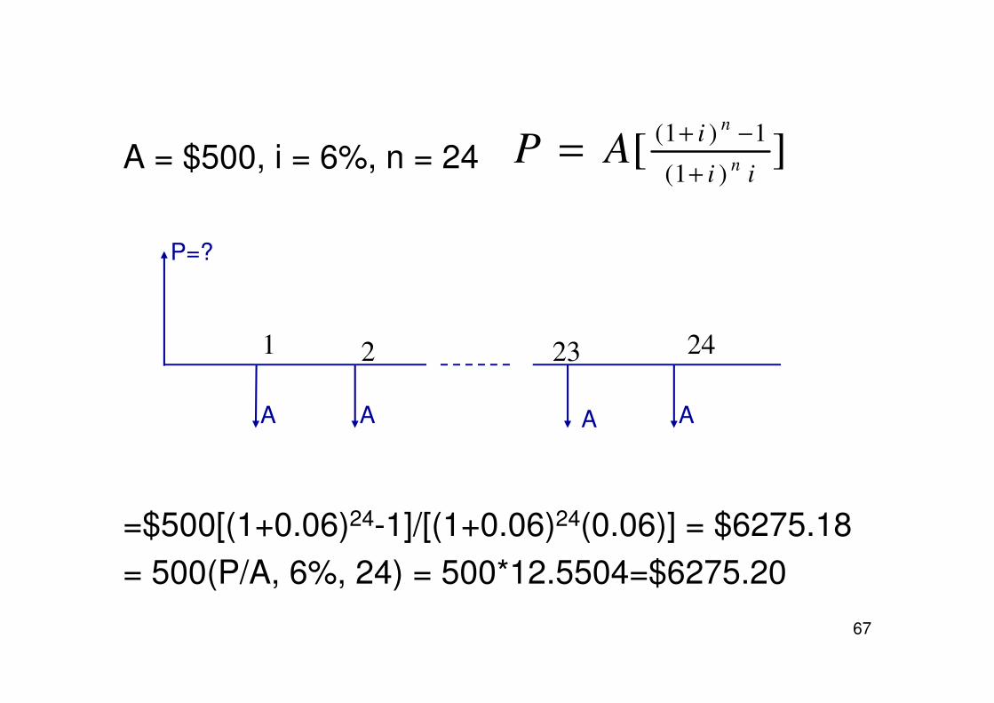
A = $500, i = 6%, n = 24
P=?
1 2 23 24
][)1(
1)1(
ii
i
n
n
AP+
−+=
67
=$500[(1+0.06)24-1]/[(1+0.06)24(0.06)] = $6275.18
= 500(P/A, 6%, 24) = 500*12.5504=$6275.20
A A A A
1 2 23 24

A A A A
1 2 23 243 220
F=?
A A
][1)1(
i
in
AF−+
=
68
=$500[(1+0.06)24-1]/0.06
=500(F/A,6%,24) = $500 * 50.815
= $ 25,407.79
A
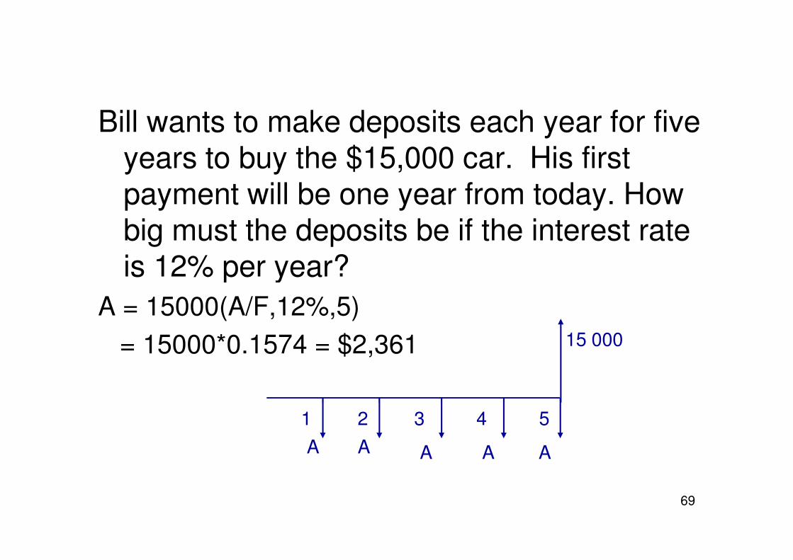
Bill wants to make deposits each year for five years to buy the $15,000 car. His first payment will be one year from today. How big must the deposits be if the interest rate is 12% per year?
69
is 12% per year?
A = 15000(A/F,12%,5)
= 15000*0.1574 = $2,361 15 000
1 2 3 4
A A A A A
5

CR = CR = القيمة السنوية المكافئة للمشروع المعطي القيمة السنوية المكافئة للمشروع المعطي
FN
0 1 2 3 N-1 N
S
(CR) Capital Cost Recovery
……….
70
استعادة رأس المال ھو عبارة عن القيمة السنوية المكافئة للكلفة ا>ولية و القيمة السنوية لقيمة
الخCص
P0
0 1 2 3 N-1 N

CR كلفة استعادة رأس المال
Given:
P0
FN
0 1 2 3 N-1 N
S
……….
71
Convert to:
0 1 2 3 N-1 N
P0
FN
$A per year (CRC)
P0
……….

Salvage for F $ at t = N
S
كلفة استعادة رأس المال
نقوم بحساب ھذه الكلفة ل\يرادات مع قيم الخ\ص
72
EAC = P(A|P, i, n) - S(A|F, i, n)
Cost = “+” and SV = “-” by conventionP
Invest P 0 $
N
Salvage for FN $ at t = N
….. … ….

كلفة استعادة رأس المال
CR = P(A|P, i, n) - S(A|F, i, n)
73
CR = P(A|P, i, n) - S(A|F, i, n)

كلفة استعادة رأس المال
اطـرح قـيـمـة الخـ\ص من –طريقة ثانيةالكـلـفـة اvصـلـيـة واحسب التكلفة السنوية
أضف للناتج الفائدة التـي تعطيھا قيمة . للفرق ، الخ\ص كل سنة SV(I) .
74
، الخ\ص كل سنة SV(I) .
CR= (P - S) (A|P, i, n) + S(i)

1. Uniform Series that are SHIFTED
• A shifted series is one whose present worth point in time is NOT t = 0.
• Shifted either to the left of t = “0” or to the right of t = “0”.
• Dealing with a uniform series:• Dealing with a uniform series:
– The PW point is always one period to the left of the first series value
– No matter where the series falls on the time line.

Example :Shifted Series
0 1 2 3 4 5 6 7 8
Consider:
A = -$500/year
P of this series is at t = 2 (P2 or F2)
P2 = $500(P/A,i%,4),
P0 = P2(P/F,i%,2)
P2P0

Consider:
0 1 2 3 4 5 6 7 8
F at t = 6
A = -$500/year
F for this series is at t = 6
F6 = A(F/A,i%,4)
P2P0

Example
F’ = $100(F/A, 15%, 3) = $347.25
F’’ = $347.25(F/P, 15%, 2) = $459.24
$1001
Cash flowYear
F5
$04
$1003
$1002
$1001

Example : Handling Time Shifts in a Uniform Series
F = ?
i = 6%
First deposit occurs at n = 0
0 1 2 3 4 5
$5,000 $5,000 $5,000 $5,000 $5,000
i = 6%
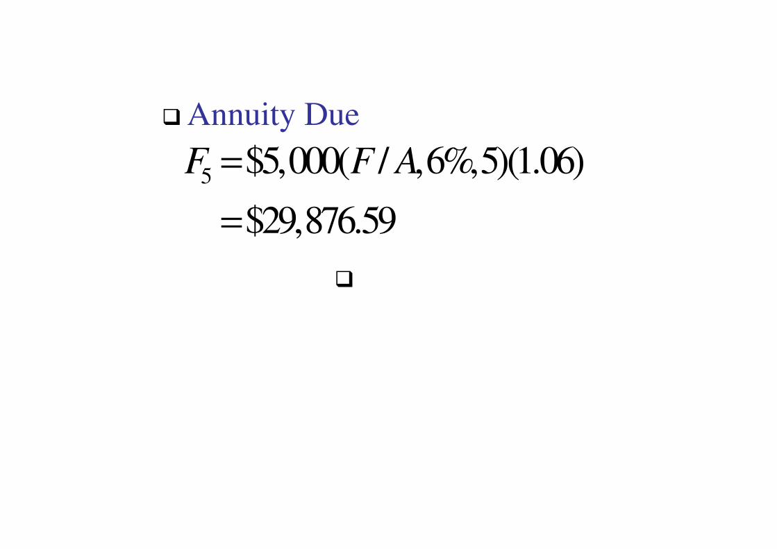
5 $5,000( / ,6%,5)(1.06)
$29,876.59
F F A=
=
� Annuity Due
��

P =$21,061.82
0 1 2 3 4 5 6
A A A A A
i = 6%
Example : Deferred Loan Repayment Plan
A A A A A
0 1 2 3 4 5 6
A’ A’ A’ A’ A’
i = 6%
P’ = $21,061.82(F/P, 6%, 1)

Two-Step Procedure
' $21,061.82( / ,6%,1)
$22,325.53
P F P=
= $22,325.53
$22,325.53( / ,6%,5)
$5,300
A A P
=
=
=

Example : Early Savings Plan – 8% interest
0 1 2 3 4 5 6 7 8 9 10
44
Option 1: Early Savings Plan
?
0 1 2 3 4 5 6 7 8 9 10 11 12
44
Option 2: Deferred Savings Plan
$2,000
$2,000 ?

Option 1 – Early Savings Plan
10 $2,000( / ,8%,10)
$28,973
F F A=
= Option 1: Early Savings Plan
?
44
$28,973
$28,973( / ,8%,34)
$396,645
F F P
=
=
=
0 1 2 3 4 5 6 7 8 9 10
44
Option 1: Early Savings Plan
$2,000
6531Age

Option 2: Deferred Savings Plan
44 $2,000( / ,8%,34)
$317,233
F F A=
=
?
$317,233=0 11 12
44
Option 2: Deferred Savings Plan
$2,000

Series with Other cash flows
• Consider:
0 1 2 3 4 5 6 7 8
A = $500
F4 = $300
0 1 2 3 4 5 6 7 8
F5 = -$400
•Find the PW at t = 0 and FW at t = 8 for this cash flow
i = 10%

The PW Points are:F4 = $300
A = $500
0 1 2 3 4 5 6 7 8
1 2 3
F5 = -$400
0 1 2 3 4 5 6 7 8
i = 10%
t = 1 is the PW point for the $500 annuity;“n” = 3

The PW Points are:F4 = $300
A = $500
0 1 2 3 4 5 6 7 8
1 2 3
Back 4 periods
F5 = -$400
0 1 2 3 4 5 6 7 8
i = 10%
t = 0 is the PW point for the two other single cash flows
Back 5 Periods

Write the Equivalence Statement
P = $500(P/A,10%,3)(P/F,10%,1)
+
$300(P/F,10%,4)
-
400(P/F,10%,5)400(P/F,10%,5)
Substituting the factor values into the equivalence expression and solving….

Substitute the factors and solve
P = $500( 2.4869 )(0.9091 )
+
$300( 0.6830 )
-
400( 0.6209 )
$1,130.42
$204.90
400( 0.6209 )
=
$1086.96
$248.36

Arithmetic Gradient Series• An arithmetic gradient is a cash flow series that
either increases or decreases by a constant amount each period
• The base amount A1 (A) is the uniform-series amount that begins in period 1 and extendsthrough period n.
91
through period n.
• Starting with the second period, each payment is greater (or smaller) than the previous one by a constant amount referred to as the arithmeticgradient G
• G can be positive or negative.

Arithmetic Gradient
We break up the cash flows into two components:
and0
30
60
90
120
A = 120
92
and1 2 3 4 5
G = 30
0
P1 P2
P1 = A (P/A,5%,5) = 120 (P/A,5%,5) = 120 (4.329) = 519P2 = G (P/G,5%,5) = 30 (P/G,5%,5) = 30 (8.237) = 247P = P1 + P2 = $766.
Note: 5 and not 4. Using 4 is a common mistake.
Standard Form Diagram for Arithmetic Gradient: n periods and n-1 nonzero flows in increasing order

Arithmetic Gradient
F = G(1+i)n-2 + 2G(1+i)n-3 + … + (n-2)G(1+i)1 + (n-1)G(1+i)0
F = G [ (1+i)n-2 + 2(1+i)n-3 + … + (n-2)(1+i)1 + n-1]
(1+i) F = G [(1+i)n-1 + 2(1+i)n-2 + 3(1+i)n-3 + … + (n-1)(1+i)1]
iF = G [(1+i)n-1 + (1+i)n-2 + (1+i)n-3 + … + (1+i)1 – n + 1] =
= G [(1+i)n-1 + (1+i)n-2 + (1+i)n-3 + … + (1+i)1 + 1] – nG =
93
= G [(1+i) + (1+i) + (1+i) + … + (1+i) + 1] – nG =
= G (F/A, i, n) - nG = G [(1+i)n-1]/i – nG
F = G [(1+i)n-in-1]/i2
P = F (P/F, i, n) = G [(1+i)n-in-1]/[i2(1+i)n]
A = F (A/F, i, n) =
= G [(1+i)n-in-1]/i2 × i/[(1+i)n-1]
A = G [(1+i)n-in-1]/[i(1+i)n-i] 0 1 2 3 …. n
G
2G
….
(n-1)G
0 …..
F

Arithmetic Gradient
Arithmetic Gradient Uniform Series
Arithmetic Gradient Present Worth
(P/G,i,n) = { [(1+i)n – i n – 1] / [i2 (1+i)n] }
(A/G,i,n) = { (1/i )– n/ [(1+i)n –1] }
=1/(G/P,i,n)
=1/(G/A,i,n)
94
(P/G,5%,5) == {[(1+i)n – i n – 1]/[i2 (1+i)n]}= {[(1.05)5 – 0.25 – 1]/[0.052 (1.05)5]}= 0.026281562/0.003190703 = 8.23691676.
(A/G,i,n) = { (1/i )– n/ [(1+i)n –1] }
(F/G,i,n) = G [(1+i)n-in-1]/i2
=1/(G/A,i,n)
=1/(G/F,i,n)

Arithmetic Gradient
Example 4-6. Maintenance costs of a machine start at $100 and go up by $100 each year for 4 years. What is the equivalent uniform annual maintenance cost for the machinery if i = 6%.
300
400
95
100
200
300
A A A A
This is not in the standard form for using the gradient equation, because the year-one cash flow is not zero.
We reformulate the problem as follows.

Arithmetic Gradient
= +A1=100
G =100
100
200
300
0
100
200
300
400
96
0
The second diagram is in the form of a $100 uniform series. The last diagram is now in the standard form for the gradient equation with n = 4, G = 100.
A = A1+ G (A/G,6%,4) =100 + 100 (1.427) = $242.70
0 1 2 3 4 0 1 2 3 4 0 1 2 3 4

Arithmetic Gradient
Example
With i = 10%, n = 4, find an equivalent uniform payment A’ for
2400018000
12000
6000
97
This is a problem with decreasing costs instead of increasing costs.
The cash flow can be rewritten as the DIFFERENCE of the following two diagrams, the second of which is in the standard form we need, the first of which is a series of uniform payments.
6000
1 2 3 40

Arithmetic Gradient
= -
18000
24000
12000
6000
A1=24000
A1 A1 A1 A13G
2G
G
G=6000
98
0 1 2 3 4 0 1 2 3 4 0 1 2 3 4
A = A1 – G(A/G,10%,4) =
= 24000 – 6000 (A/G,10%,4) =
= 24000 – 6000(1.381) = 15,714.
Arithmetic Gradient
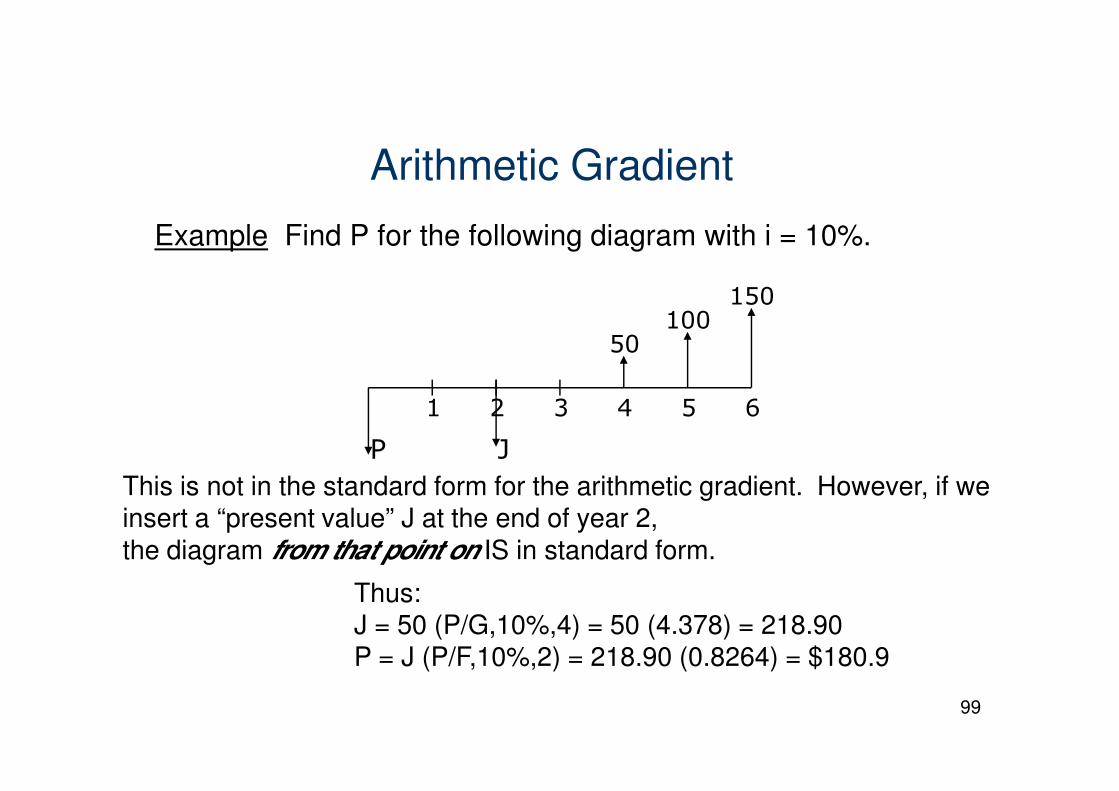
Example Find P for the following diagram with i = 10%.
1 2 3 4 5 6
50
100
150
99
P
1 2 3 4 5 6
This is not in the standard form for the arithmetic gradient. However, if we insert a “present value” J at the end of year 2, the diagram from that point on IS in standard form.
J
Thus: J = 50 (P/G,10%,4) = 50 (4.378) = 218.90P = J (P/F,10%,2) = 218.90 (0.8264) = $180.9