engineering characteristics of sensitive marine … characteristics of sensitive marine clays -...
TRANSCRIPT

Engineering Characteristics of Sensitive Marine
Clays - Examples of Clays in Eastern Canada
by
Athir Nader
Thesis submitted to the
Faculty of Graduate and Postdoctoral Studies
In partial fulfillment of the Requirements
For the M.A.Sc degree in Civil Engineering
Civil Engineering Department
Faculty of Engineering
University Of Ottawa
© Athir Nader, Ottawa, Canada, 2014

Engineering Characteristics of Sensitive Marine
Clays - Examples of Clays in Eastern Canada
Submitted by
Athir Nader
In partial fulfillment of the requirements for the degree of
Master of Science
in
Civil Engineering
____________________________
Prof. M. Fall
(Thesis supervisor)

iii
Contents
List of Figures ......................................................................... viii
List of Tables .......................................................................... xvii
List of Symbols ....................................................................... xix
Abstract .................................................................................... xx
Acknowledgement .................................................................. xxii
Chapter 1: Introduction ............................................................... 1
1.1 Problem Statement ................................................................................................................ 1
1.2 Research Objectives .............................................................................................................. 2
1.3 Thesis Organization............................................................................................................... 3
Chapter 2: Technical and Theoretical Background ..................... 5
2.1 Background on Sensitive Marine Clays in Canada ............................................................... 5
2.1.1 Geology and Distribution of Sensitive Marine Clays in Canada.................................... 5
2.1.1.1 Origin and Distribution of Sensitive Marine Clays in Canada ................................. 5
2.1.1.2 Sedimentology of Sensitive Marine Clay ................................................................. 9
2.1.2 Chemical, Mineralogical and Structural Characteristics of Sensitive Marine Clays ... 12
2.1.2.1 Mineralogical characteristics .................................................................................. 12
2.1.2.2 Porewater chemistry................................................................................................ 13
2.1.2.3 Structure of Sensitive Marine Clay ......................................................................... 18
2.2 Background on Cone and Ball Penetrometers..................................................................... 20
2.2.1 Introduction .................................................................................................................. 20
2.2.2 Background on Cone Penetration Testing .................................................................... 21
2.2.2.1 Undrained Shear Strength ....................................................................................... 21
2.2.2.2 Sensitivity ............................................................................................................... 22
2.2.2.3 Soil Classification ................................................................................................... 22

iv
2.2.2.4 Preconsolidation Pressure and OCR ....................................................................... 23
2.2.2.5 Pore Pressure Dissipation Tests .............................................................................. 24
2.2.2.6 Seismic Cone Testing ............................................................................................. 25
2.2.2.7 Geostratification ...................................................................................................... 26
2.2.3 Background on ball penetrometers ............................................................................... 28
2.2.3.1 Penetration Resistance Correction .......................................................................... 29
2.2.3.2 Undrained Shear Strength ....................................................................................... 29
2.3 Correlations from the Canadian Foundation Engineering Manual ..................................... 29
2.4 Summary and Conclusion ................................................................................................... 31
2.5 References ........................................................................................................................... 32
Chapter 3: Technical Paper I - Geotechnical Properties of
Sensitive Marine Clays - Examples of Clays in Eastern Canada
.................................................................................................. 41
Abstract ..................................................................................................................................... 41
Keywords ................................................................................. 42
3.1 Introduction ......................................................................................................................... 42
3.2 Geographical and Geological Characteristics ..................................................................... 43
3.2.1 The Sites ....................................................................................................................... 43
3.2.2 Origin and Geological Setting ...................................................................................... 48
3.2.3 Porewater Chemistry .................................................................................................... 50
3.2.4 Mineralogical Composition of Sensitive Marine Clay ................................................. 51
3.3 Physical Characteristics, Atterberg Limits and Activity ..................................................... 52
3.3.1 Physical Characteristics ................................................................................................ 52
3.3.1.1 Void ratio and porosity ........................................................................................... 52
3.3.1.3 Unit Weight ............................................................................................................. 53
3.3.1.4 Clay Fraction ........................................................................................................... 54

v
3.3.1.5 Specific Gravity ...................................................................................................... 55
3.3.2 Atterberg Limits and Water Content ............................................................................ 56
3.3.3 Activity ......................................................................................................................... 63
3.4 Geotechnical In-Situ Tests on Sensitive Marine Clay in Ottawa ........................................ 64
3.4.1 Cone Penetration Tests ................................................................................................. 64
3.4.2 Standard Penetration Tests ........................................................................................... 71
3.4.3 Vane Shear Tests and Undrained Shear Strength ......................................................... 73
3.4.4 FVTs and LVTs ......................................................................................................... 79
3.4.5 Shear Wave Velocity Measurements ............................................................................ 82
3.5 Interface Shear Strength and Behavior................................................................................ 86
3.6 Consolidation Behavior ....................................................................................................... 88
3.6.1 Preconsolidation Pressure and Over Consolidation Ratio ............................................ 88
3.6.2 Compression Index ....................................................................................................... 90
3.6.2.1 Example of Consolidation Curve ............................................................................ 91
3.6.2 Recompression Index ................................................................................................... 92
3.6.3 Coefficient of Consolidation ........................................................................................ 94
3.6.4 Secondary Compression Index ................................................................................... 104
3.7 Sensitivity of Marine Clay in Ottawa ................................................................................ 107
3.8 Hydraulic Conductivity ..................................................................................................... 113
3.9 Summary and Conclusion ................................................................................................. 121
Acknowledgement ................................................................................................................... 122
3.10 References ....................................................................................................................... 123
Chapter 4: Technical Paper II - Characterization of Sensitive
Marine Clays by Using Cone and Ball Penetrometers –
Examples of Clays in Eastern Canada .................................... 131
Abstract ................................................................................................................................... 131

vi
Keywords ................................................................................................................................ 132
4.1 Introduction ....................................................................................................................... 132
4.2 Site description .................................................................................................................. 134
4.2.1 Geographical location ................................................................................................. 134
4.2.2 Geological characteristics ........................................................................................... 135
4.3 Experimental Programs and Soil Characterization ........................................................... 136
4.3.1 Field testing programs ................................................................................................ 136
4.3.1.1 CPT Tests .............................................................................................................. 136
4.3.1.2 Ball Penetrometers ................................................................................................ 136
4.3.1.3 Field Vane Shear Tests ......................................................................................... 136
4.3.1.4 Drilling and sampling ........................................................................................... 136
4.3.1.5 Wells installation .................................................................................................. 137
4.3.1.6 Geodetic Elevations and coordinates .................................................................... 139
4.3.2 Laboratory testing programs and soil characterization ............................................... 139
4.3.2.1 Unit weight, moisture content, and specific gravity ............................................. 139
4.3.2.2 Grain size distribution and soil index properties .................................................. 140
4.3.2.3 Preconsolidation Pressure ..................................................................................... 142
4.3.2.4 Porewater Chemistry ............................................................................................. 143
4.3.2.5 Cone Equipment Calibration and Temperature Effects ........................................ 144
4.4 Results of the penetrometer tests and discussion .............................................................. 149
4.4.1 Soil Specific Cone Factors ......................................................................................... 149
4.4.1.1 Cone Penetrometer ................................................................................................ 149
4.4.1.2 Ball Penetrometers ................................................................................................ 154
4.4.2 Sensitivity Estimation ................................................................................................. 157
4.4.3 Soil Geotechnical profile ............................................................................................ 161

vii
4.4.4 Consolidation History ................................................................................................. 163
4.5 Summary and conclusions ................................................................................................. 165
Acknowledgement ................................................................................................................... 167
4.6 References ......................................................................................................................... 167
Chapter 5 Conclusions and Recommendations ....................... 179
5.1 Summary ........................................................................................................................... 179
5.2 Conclusions and Future Research Recommendations ...................................................... 179
5.3 References ......................................................................................................................... 183
6 Appendixes .......................................................................... 184
6.1 Appendix #1: Implementation Practice Guide for CPTs for Stantec Consulting Limited 184
6.1.1 Cone Penetration Test Equipment .............................................................................. 184
6.1.2 Field Implementation .................................................................................................. 184
6.1.3 Data Reduction and Interpretation .............................................................................. 187
6.1.3.1 CPT ....................................................................................................................... 187
6.1.3.2 Seismic Profile ...................................................................................................... 188
6.1.3.3 Dissipation Test .................................................................................................... 190
6.1.4 References .................................................................................................................. 193
6.2 Appendix #2: Field Photos for Canadian Geotechnical Research Site No. 1 ................... 194
6.3 Appendix #3: Lab Graphs for Canadian Geotechnical Research Site No. 1 ..................... 201
6.4 Appendix #4: Coefficient of Consolidation from Consolidation and CPT Dissipation
Testing ..................................................................................................................................... 203
6.4.1 Cv from Taylor's Square Root of Time Fitting Method .............................................. 203
6.4.2 Cv from Dissipation Testing....................................................................................... 204
6.4.3 References .................................................................................................................. 205

viii
List of Figures
FIGURE 1-1 SCHEMATIC DIAGRAM THAT ILLUSTRATES THE ORGANIZATION OF
THE THESIS .......................................................................................................................... 4
FIGURE 2-1 WISCONSIN ICE SHEET (ABER 2005) ................................................................ 6
FIGURE 2-2 GLACIAL AND MARINE DISTRIBUTION IN CANADA (QUIGLEY 1980) .... 6
FIGURE 2-3 11800 YEARS ICE FRONT AND LAKE AGASSIZ, LAKE ALGONQUIN, AND
CHAMPLAIN SEA (QUIGLEY 1980) .................................................................................. 7
FIGURE 2-4 IBERVILLE SEA, TYRRELL SEA, LE FLAMME SEA, LAKE BARLOW-
OJIBWAY, AND LAKE AGASSIZ (QUIGLEY 1980) ........................................................ 9
FIGURE 2-5 SUMMER HEAVY DENSITY FLOW INTO GLACIAL LAKES (QUIGLEY
1980) ..................................................................................................................................... 10
FIGURE 2-6 WINTER OVERFLOW INTO GLACIAL LAKES (QUIGLEY 1980)................. 10
FIGURE 2-7 WATER CONTENT PROFILE FOR VARVED CLAY (LEROUEIL 1999) ....... 11
FIGURE 2-8 IRON AND ALUMINUM OXIDES VERSES DEPTH (BERRY 1988) .............. 13
FIGURE 2-9 BORING PROFILE OF CATION CONCENTRATION AND OTHER
PARAMETERS FOR TREADWELL-OTTAWA WHERE ST IS THE SENSITIVITY
(TORRANCE 1979) ............................................................................................................. 15
FIGURE 2-10 BORING PROFILE OF CATION CONCENTRATION AND OTHER
PARAMETERS FOR TOURAINE-OTTAWA WHERE ST IS THE SENSITIVITY
(TORRANCE 1979) ............................................................................................................. 16
FIGURE 2-11 DOUBLE LAYER CONCEPT ............................................................................. 19
FIGURE 2-12 EXAMPLE DISSIPATION TEST (MAYNE 2009) ............................................ 29
FIGURE 2-13 SHEAR WAVE ARRIVAL (MAYNE 2009)....................................................... 29
FIGURE 2-14 CPT RESULTS FOR NEW ORLEANS SOIL (MAYNE 2009) .......................... 29
FIGURE 2-15 SOIL IDENTIFICATION USING SOIL BEHAVIOR TYPE (LUNNE ET AL.
1997) ..................................................................................................................................... 29
FIGURE 3-1 SITES LOCATIONS MAP OBTAINED FROM GOOGLE EARTH ................... 44
FIGURE 3-2 STRATIFICATION FOR (A) SITE 1 (B) SITE 2 (C) SITE 3 (D) SITE 4 (E) SITE
5 (F) SITE 6 (G) SITE 7 (H) SITE 8 (I) SITE 9 (J) SITE 10 (K) SITE 11 (L) SITE 12 (M)
SITE 13 ................................................................................................................................. 48

ix
FIGURE 3-3 CHLORIDE, SULPHATE, RESISTIVITY, AND PH WITH DEPTH .................. 51
FIGURE 3-4 VOID RATIO AND POROSITY WITH DEPTH .................................................. 53
FIGURE 3-5 UNIT WEIGHT WITH DEPTH ............................................................................. 54
FIGURE 3-6 SPECIFIC GRAVITY WITH DEPTH ................................................................... 56
FIGURE 3-7 MOISTURE CONTENTS, LIQUID LIMITS, PLASTIC LIMITS, AND
PLASTICITY INDEX WITH DEPTH FOR (A) SITE 1 (B) SITE 2 (C) SITE 3 (D) SITE 4
(E) SITE 5 (F) SITE 7 (G) SITE 8 (H) SITE 9 (I) SITE 10 (J) SITE 11 (K) SITE 12 (L)
SITE 13 (M) SITE 14 (N) SITE 15 (O) SITE 6 ................................................................... 62
FIGURE 3-8 CASSAGRANDE'S PLASTICITY CHART FOR PLASTICITY PROPERTIES
OF ALL SITES EXCEPT FOR SITE 6 ................................................................................ 63
FIGURE 3-9 ACTIVITY CHART ............................................................................................... 64
FIGURE 3-10 TIP RESISTANCE, SLEEVE FRICTION, AND POREWATER PRESSURE
WITH DEPTH FOR (A) SITE 1 (B) SITE 2 (C) SITE 3 (D) SITE 5 (E) SITE 7 (F) SITE 8
(G) SITE 9 (H) SITE 10 (I) SITE 11 .................................................................................... 70
FIGURE 3-11 TIP RESISTANCE AND POREWATER PRESSURE WITH DEPTH FOR (A)
SITE 6 (B) SEWAGE WATER TREATMENT PLANT IN OTTAWA PERFORMED BY
KONRAD AND LAW (1987) .............................................................................................. 71
FIGURE 3-12 N60 FROM SPT WITH DEPTH FOR(A) SITE 1 (B) SITE 2 (C) SITE 3 (D) SITE
4 (E) SITE 5 (F) SITE 7 (G) SITE 8 (H) SITE 9 (I) SITE 10 (J) SITE 11 (K) SITE 12 (L)
SITE 13 (M) SITE 14 (N) SITE 15 ...................................................................................... 73
FIGURE 3-13 UNDRAINED SHEAR STRENGTH FROM FIELD VANES TESTS (FVT),
LAB VANES TESTS (LVT), AND/OR SPT CORRELATION FOR (A) SITE 1 (B) SITE 2
(C) SITE 3 (D) SITE 4 (E) SITE 5 (F) SITE 7 (G) SITE 8 (H) SITE 9 (I) SITE 10 (J) SITE
11 (K) SITE 12 (L) SITE 13 (M) SITE 14 (N) SITE 15 ...................................................... 79
FIGURE 3-14 NILCON FIELD VANES AND MINIATURE LAB VANES RESULTS FOR
SITE 6 (A) UNDRAINED SHEAR STRENGTH WITH DEPTH (B) REMOLDED SEHAR
STRENGTH WITH DEPTH (C) SENSITIVITY WITH DEPTH ....................................... 81
FIGURE 3-15 REMOLDED SHEAR STRENGTH WITH ROTATION ANGLE FROM
NILCON FIELD VANES FOR ROTATIONAL RATE OF 0.1 DEGREE/S FOR SITE 6
AT A DEPTH OF (A) 3.68 M AND (B) 16.68 M ................................................................ 81
x
FIGURE 3-16 SHEAR WAVE VELOCITY AND SHEAR STRENGTH WITH DEPTH AND
SITE CLASSIFICATION ACCORDING TO THE CANADIAN ENGINEERING
FOUNDATION MANUAL FOR (A) SITE 7 (B) SITE 7 (C) SITE 8 (D) SITE 8 (E) SITE 9
(F) SITE 9 (G) SITE 9 (H) SITE 9 (I) SITE 9 (J) SITE 9 (K) SITE 9 (L) SITE 9 (M) SITE 9
(N) SITE 9............................................................................................................................. 86
FIGURE 3-17 (A) PRECONSOLIDATION PRESSURE WITH DEPTH (B) OCR WITH
DEPTH FOR ALL SITES .................................................................................................... 90
FIGURE 3-18 COMPRESSION INDEX WITH DEPTH ............................................................ 91
FIGURE 3-19 CONSOLIDATION CURVE FOR A DEPTH OF 3.8 M FROM SITE 6 ........... 92
FIGURE 3-20 RECOMPRESSION INDEX WITH DEPTH FROM OEDOMETER TESTS .... 93
FIGURE 3-21 CONSOLIDATION CURVE AND THE COEFFICIENT OF CONSOLIDATION
WITH PRESSURE FROM OEDOMETER TESTS FOR SITE 2 FOR A DEPTH OF (A)
3.43 M (B) 8.0 M (C) 4.95 M (D) 9.45 (E) 3.58 M (F) 12.42 M AND FOR SITE 3 FOR A
DEPTH OF (G) 3.43 M (H) 8.0 M (I) 4.95 M (J) 9.45 (K) 3.58 M (L) 12.42 M ................. 98
FIGURE 3-22 COEFFICIENT OF CONSOLIDATION WITH STRESS FROM OEDOMETER
TESTS FOR A DEPTH OF (A) 2.6 M SITE 6 (B) 4.1 M SITE 6 (C) 6.4 M SITE 6 (D) 8.7
M SITE 6 (E) 12.6 M SITE 6 (F) 14.0 M SITE 6 (G) 15.5 M SITE 6 (H) 17.1 M SITE 6 (I)
18.6 M SITE 6 (J) 9.1 M SITE 2 (K) 12.2 M SITE 3 (L) 12.2 M SITE 4 (M) 13.7 M SITE 4
(N) 13.7 M SITE 8 (O) 7.6 M SITE 9 (P) 7.6 M SITE 10 (Q) 10.7 M SITE 10 (R) 7.8 M
SITE 11 (S) 16.5 M SITE 11 (T) 11.0 M SITE 13 (U) 4.6 M SITE 13 (V) 4.8 M SITE 13
............................................................................................................................................. 101
FIGURE 3-23 SECONDARY COMPRESSION INDEX WITH DEPTH FROM OEDOMETER
TESTS ................................................................................................................................. 105
FIGURE 3-24 EXAMPLE DIAL READING WITH TIME FROM OEDOMETER TEST FOR
SAMPLE FROM OTTAWA .............................................................................................. 107
FIGURE 3-25 SENSITIVITY WITH DEPTH FOR (A) SITE 1 (B) SITE 2 (C) SITE 3 (D) SITE
4 (E) SITE 5 (F) SITE 7 (G) SITE 8 (H) SITE 9 (I) SITE 10 (J) SITE 11 (K) SITE 12 (L)
SITE 13 (M) SITE 14 (N) SITE 15 .................................................................................... 113
FIGURE 3-26 COEFFICIENT OF PERMEABILITY WITH STRESS FROM OEDOMETER
TESTS FOR A DEPTH OF (A) 2.6 M SITE 6 (B) 4.1 M SITE 6 (C) 6.4 M SITE 6 (D) 8.7
M SITE 6 (E) 12.6 M SITE 6 (F) 14.0 M SITE 6 (G) 15.5 M SITE 6 (H) 17.1 M SITE 6 (I)

xi
18.6 M SITE 6 (J) 9.1 M SITE 2 (K) 12.2 M SITE 3 (L) 12.2 M SITE 4 (M) 13.7 M SITE 4
(N) 13.7 M SITE 8 (O) 7.6 M SITE 9 (P) 7.6 M SITE 10 (Q) 10.7 M SITE 10 (R) 7.8 M
SITE 11 (S) 16.5 M SITE 11 (T) 11.0 M SITE 13 (U) 4.6 M SITE 13 (V) 4.8 M SITE 13
............................................................................................................................................. 117
FIGURE 3-27 HYDRAULIC CONDUCTIVITY WITH DEPTH FOR SITE 6 SUPPLIED BY
NATIONAL RESEARCH COUNCIL CANADA AND REPORTED BY HINCHBERGER
AND ROWE (1998) ........................................................................................................... 120
FIGURE 4-1 GEOGRAPHICAL LOCATION OF THE CANADIAN GEOTECHNICAL
RESEARCH SITE NO. 1 ................................................................................................... 134
FIGURE 4-2 WATER TABLE GEODETIC ELEVATIONS WITH DATES FROM THE
MULTILEVEL MONITORING WELLS .......................................................................... 138
FIGURE 4-3 POREWATER PRESSURE READINGS FROM CONE, 40 MM BALL, AND 113
MM BALL TIPS AND HYDROSTATIC POREWATER PRESSURE WITH GEODETIC
ELEVATIONS, CPT-1 AND CPT-2 ARE POREWATER PRESSURE READINGS FROM
CONE TIP TESTS 1 AND 2, 40-BALL-1 AND 40-BALL-2 ARE POREWATER
PRESSURE READINGS FROM 40 MM BALL TIP TESTS 1 AND 2, 113-BALL IS
POREWATER PRESSURE READINGS FROM 113 MM BALL TIP TEST, HPP IS
HYDROSTATIC POREWATER PRESSURE READINGS FROM MONITORING
WELLS READINGS .......................................................................................................... 138
FIGURE 4-4 (A) UNIT WEIGHT WITH GEODETIC ELEVATIONS (B) MOISTURE
CONTENT WITH GEODETIC ELEVATIONS (C) SPECIFIC GRAVITY WITH
GEODETIC ELEVATIONS ............................................................................................... 140
FIGURE 4-1 (A) PERCENTAGE PARTICLES SIZE WITH GEODETIC ELEVATIONS
(COLLOIDS <0.001 MM, CLAY 0.001- 0.005 MM, SILT 0.005-0.075, SAND 0.075-
0.04.75 MM, GRAVEL 4.75-75 MM) (B) PLASTICITY INDEX WITH GEODETIC
ELEVATIONS (C) MOISTURE CONTENT WITH GEODETIC
ELEVATIONS.......................................152
FIGURE 4-2 MOISTURE CONTENTS, PLASTIC LIMITS, AND LIQUID LIMITS WITH
GEODETIC ELEVATIONS, PL IS THE PLASTIC LIMITS, LL IS THE LIQUID LIMIT,
MC IS THE MOISTURE CONTENT................................................153

xii
FIGURE 4-7 (A) PRECONSOLIDATION PRESSURE WITH GEODETIC ELEVATIONS (B)
OVERCONSOLIDATION RATIO WITH GEODETIC ELEVATIONS ......................... 143
FIGURE 4-8 (A) CHLORIDE CL ANIONS (B) CALCIUM CA CATIONS (C) MAGNESIUM
MG CATIONS (D) POTASSIUM K CATIONS (E) SODIUM NA CATIONS WITH
GEODETIC ELEVATIONS ............................................................................................... 144
FIGURE 4-9 (A) TIP STRESS GAIN WITH TEMPERATURE CHANGE DUE TO HEATING
(B) TIP STRESS LOSS WITH TEMPERATURE CHANGE DUE TO COOLING ........ 145
FIGURE 4-10 (A) SLEEVE FRICTION STRESS GAIN WITH TEMPERATURE CHANGE
DUE TO HEATING (B) SLEEVE FRICTION STRESS LOSS WITH TEMPERATURE
CHANGE DUE TO COOLING ......................................................................................... 146
FIGURE 4-11 (A) POREWATER PRESSURE LOSS WITH TEMPERATURE CHANGE DUE
TO HEATING (B) POREWATER PRESSURE GAIN WITH TEMPERATURE CHANGE
DUE TO COOLING ........................................................................................................... 146
FIGURE 4-12 TEMPERATURE PROFILE FROM THREE PENETROMETERS TESTS ..... 149
FIGURE 4-13 CONE PENETRATION TESTS RESULTS WITH GEODETIC ELEVATIONS
FOR (A) TIP RESISTANCE (B) SLEEVE FRICTION (C) POREWATER PRESSURE,
QT1 AND QT2 ARE TIP RESISTANCES FOR TESTS 1 AND 2, FS1 AND FS2 ARE
SLEEVE FRICTIONS FOR TESTS 1 AND 2, U2(1) AND U2(2) ARE POREWATER
PRESSURES FOR TESTS 1 AND 2 ................................................................................. 150
FIGURE 4-14 CONE SOIL SPECIFIC FACTORS AND PLASTICITY INDEX WITH
GEODETIC ELEVATIONS, NKT1 AND NKT2 ARE CONE SOIL SPECIFIC FACTORS
FROM CORRECTED TIP RESISTANCE FOR CONE TESTS 1 AND 2, NK1 AND NK2
ARE CONE SOIL SPECIFIC FACTORS FROM UNCORRECTED TIP RESISTANCE
FOR CONE TESTS 1 AND 2, NΔU1 AND NΔU2 ARE CONE SOIL SPECIFIC
FACTORS FROM EXCESS POREWATER PRESSURE FOR CONE TESTS 1 AND 2 152
FIGURE 4-15 (A) CONE SOIL SPECIFIC FACTOR NKT FROM CORRECTED TIP
RESISTANCE WITH POREWATER PRESSURE RATIO (B) CONE SOIL SPECIFIC
FACTOR NK FROM UNCORRECTED TIP RESISTANCE WITH PLASTICITY
INDEX(C) CONE SOIL SPECIFIC FACTOR NU FROM EXCESS POREWATER
PRESSURE WITH POREWATER PRESSURE RATIO .................................................. 153

xiii
FIGURE 4-16 NET TIP RESISTANCE WITH GEODETIC ELEVATIONS FOR (A) 40 MM
BALL TIP (B) 113 MM BALL TIP, QB1 AND QB2 ARE NET TIP RESISTANCES FOR
40 MM TIP TESTS 1 AND 2, QB(113MM) IS NET TIP RESISTANCE FOR 113MM
BALL TIP TEST................................................................................................................. 154
FIGURE 4-17 (A) BALL SOIL SPECIFIC FACTOR NSU-113-BALL FOR 113 MM BALL
TIP WITH GEODETIC ELEVATION (B) BALL SOIL SPECIFIC FACTOR FOR 40 MM
BALL TIP WITH GEODETIC ELEVATION, NSU1 AND NSU2 ARE BALL SOIL
SPECIFIC FACTORS FOR 40 MM BALL TESTS 1 AND 2 ................ 157FIGURE 4-3 (A)
UNDRAINED SHEAR STRENGTH WITH GEODETIC ELEVATIONS FROM FIELD
VANE TESTS (B) SENSITIVITY WITH GEODETIC ELEVATIONS FROM FIELD
VANE TESTS, SU IS THE INITIAL UNDRAINED SHEAR STRENGTH, SUR IS THE
REMOLDED UNDRAINED SHEAR
STRENGTH...............................................................169
FIGURE 4-4 (A) SENSITIVITY FROM CONE PENETRATION TESTS 1 AND 2 ST(CPT-1)
AND ST(CPT-2) AND FROM FIELD VANE TESTS ST(FVT) WITH GEODETIC
ELEVATIONS (B) SENSITIVITY FROM CONE PENETRATION TEST CPT WITH
SENSITIVITY FROM FIELD VANE TESTS FVT (C) SLEEVE FRICTION WITH TIP
RESISTANCES FROM CONE PENETRATION
TESTS...........................................................................................................................171
FIGURE 4-20 (A) SENSITIVITY FACTOR NS FROM CONE PENETRATION TESTS 1 AND
2 CPT-1 AND CPT-2 (B) PLASTICITY INDEX WITH GEODETIC ELEVATIONS FOR
THE PURPOSE OF COMPARISON ................................................................................. 161
FIGURE 4-21 (A) SOIL TYPE CLASSIFICATION ACCORDING TO JEFFERIES AND
DAVIES (1991) FOR CONE PENETRATION TEST 1 WITH GEODETIC ELEVATIONS
(B) SOIL TYPE CLASSIFICATION ACCORDING TO JEFFERIES AND DAVIES
(1991) FOR CONE PENETRATION TEST 2 WITH GEODETIC ELEVATIONS (C) SOIL
TYPE ACCORDING TO CASSAGRANDE'S PLASTICITY CHART CPC FROM
PLASTICITY RESULTS WITH GEODETIC ELEVATIONS, HORIZONTAL AXIS IS
THE SOIL CLASS NUMBER OR NUMBER REPRESENTING THE SOIL NAME ..... 162

xiv
FIGURE 4-22 FINES CONTENT ACCORDING TO THE METHOD SUGGESTED BY
LUNNE ET. AL. (1997) FROM CONE PENETRATION TESTS 1 AND 2 FC(CPT-1)
AND FC(CPT-2) AND FROM LABORATORY TESTING FC WITH GEODETIC
ELEVATIONS .................................................................................................................... 163
FIGURE 4-5 (A) NORMALIZED TIP RESISTANCE FROM CONE PENETRATION TESTS 1
AND 2 QT(CPT-1) AND QT(CPT-2) WITH GEODETIC ELEVATIONS (B)
OVERCONSOLIDATION RATIO FROM LABORATORY TESTING WITH GEODETIC
ELEVATION FOR THE PURPOSE OF COMPARISON (C) K FACTOR FOR
CONSOLIDATION HISTORY FROM CONE PENETRATION TESTS 1 AND 2 K(CPT-1)
AND K(CPT-2) WITH GEODETIC
ELEVATIONS...................................................................................................................................
............................176
FIGURE 4-24 OVERCONSOLIDATION RATIO FROM LABORATORY TESTING WITH
(A) NORMALIZED TIP RESISTANCE FROM CONE PENETRATION TESTS 1 AND 2
QT(CPT-1) AND QT(CPT-2) (B) POREWATER PRESSURE RATIO FROM CONE
PENETRATION TESTS 1 AND 2 BQ(CPT-1) AND BQ(CPT-2) ................................... 165
FIGURE 6-1 BASELINE AND TEST READINGS IN MV IN THE DATA FILE OBTAINED
FROM DAS FOR STANTEC CPT EQUIPMENT ............................................................ 188
FIGURE 6-2 DATA FILE FOR SEISMIC TESTING OBTAINED FROM STANTEC CPT
EQUIPMENT, THE FILE SHOWS WHERE THE TEST DEPTH, DURATION, AND
AMPLITUDES CAN BE FOUND ..................................................................................... 189
FIGURE 6-3 PLOT OF WAVE AMPLITUDE VERSES TIME, THE PLOT SHOWS THE
ESTIMATED ARRIVAL TIME OF THE SHEAR WAVE .............................................. 190
FIGURE 6-4 DATA FILE FOR DISSIPATION TESTING OBTAINED FROM STANTEC CPT
EQUIPMENT, THE FILE SHOWS WHERE THE TEST DEPTH, DURATION, AND
POREWATER PRESSURE CAN BE FOUND ................................................................. 191
FIGURE 6-5 EXAMPLE OF T50 DETERMINATION FROM POREWATER PRESSURE
VERSES TIME ................................................................................................................... 192
FIGURE 6-6 EXAMPLE DETERMINATION OF CH FROM T50 (ROBERTSON ET AL. 1990)
............................................................................................................................................. 192

xv
FIGURE 6-7 (A) THE MAIN RESEARCHER BY SITE SIGN WITH DRILL RIG AND CPT
VAN IN BACKGROUND (B) POINTS BEING SURVEYED USING GPS (C) SITE
GATE AND SITE CONDITION PRIOR TO TESTING ................................................... 194
FIGURE 6-8 (A) THE MAIN RESEARCHER INSIDE PENETROMETER VAN WITH
PENETROMETER DATA ACQUISITION SYSTEM AND PUSH RODS (B) CONE TIP
ATTACHED TO THE PROBE (C) 40 MM BALL TIP ATTACHED TO THE PROBE. 195
FIGURE 6-9 (A) 40 MM BALL TIP ATTACHED TO THE PENETROMETER PROBE (B)
113 MM BALL TIP ATTACHED TO THE PROBE (C) MAIN RESEARCHER WITH 113
MM BALL TIP ATTACHED TO THE PENETROMETER PROBE ............................... 196
FIGURE 6-10 (A) PENETROMETER PUSH RODS BEING PULLED OUT OF THE
GROUND AFTER COMPLETION OF TESTING (B) PENETROMETER DEPTH
TRANSDUCER BOX MOUNTED ON DRILL RIG TO MEASURE THE PUSH DEPTH
(C) AVAILABLE SIZES OF FIELD (NILCON VANES) ................................................ 197
FIGURE 6-11 (A) MEDIUM SIZE VANE ATTACHED TO THE VANE PUSH ROD (B)
ELECTRONIC VANE MOTOR MOUNTED ON THE DRILLING AUGERS AND
CLIPPED TO THE VANE PUSH RODS FOR TESTING (C) DRILLING AUGERS..... 198
FIGURE 6-12 (A) PISTON SAMPLER ATTACHED TO THE DRILL RIG FOR
UNDISTURBED SOIL SAMPLING USING SHELBY TUBES (B) SHELBY TUBE
ATTACHED TO THE PISTON SAMPLER WITH BAGS OF SAND AND BENTONITE
FOR SEALING AROUND PIEZOMETER (C) SHELBY TUBE WITH SAMPLE JUST
BEING PULLED OUT OF THE GROUND (D) MAIN RESEARCHER WITH
UNDISTURBED SAMPLE IN A SHELBY TUBE .......................................................... 199
FIGURE 6-13 (A) SHELBY TUBE BEING WAXED FROM THE ENDS THE CAPED TO
PREVENT MOISTURE TRANSFER (B) FLOWING SENSITIVE MARINE CLAY IN
OTTAWA WHEN DISTURBED (C) SCREEN ATTACHED AT THE END OF TUBE
ACTING AS PIEZOMETER TO MEASURE THE HYDROSTATIC WATER PRESSURE
AT DIFFERENT LEVELS (D) PIEZOMETER BEING DROPPED INTO THE GROUND
TO MEASURE THE HYDROSTATIC WATER PRESSURE ......................................... 200
FIGURE 6-14 (A) CONSOLIDATION GRAPH AT 2.3 M DEPTH (B) CONSOLIDATION
GRAPH AT 3.8 M DEPTH (C) CONSOLIDATION GRAPH AT 16.8

xvi
MDEPTH...........................................................................................................................................
..............214
FIGURE 6-15 GRAIN SIZE DISTRIBUTION FOR SAMPLE DEPTHS FROM 2.4 TO 19.8 202
FIGURE 6-16 EXAMPLES OF DIAL READING WITH SQUARE ROOT OF TIME FOR A
STAGE OF OEDOMETER LOADING FOR SAMPLES FROM OTTAWA (A) DOUBLE
LOADING INCREMENTS (B) RANDOM LOADING INCREMENTS ......................... 203
FIGURE 6-17 COEFFICIENT OF CONSOLIDATION FROM DISSIPATION TESTS FROM
CPT ..................................................................................................................................... 205

xvii
List of Tables
TABLE 2-1 TABLE 3.3 FROM THE CANADIAN FOUNDATION ENGINEERING
MANUAL ............................................................................................................................. 30
TABLE 2-2 TABLE 6.1A FROM THE CANADIAN FOUNDATION ENGINEERING
MANUAL 2005 .................................................................................................................... 30
TABLE 3-1 CLAY FRACTIONS WHERE EACH VALUES REPRESENTS A
LABORATORY TEST ......................................................................................................... 55
TABLE 3-2 NKT, NK, NΔU, AND DISTANCE TO REFERENCE FIELD VANES .................... 65
TABLE 3-3 COMPRESSION INDEX TO RECOMPRESSION INDEX RATIOS .................... 94
TABLE 3-4 SUMMARY OF T90 AND THE COEFFICIENT OF CONSOLIDATION
RELATIVE TO THE STRESS INTERVAL, DEPTH, AND PRECONSOLIDATION
PRESSURE FROM OEDOMETER TESTS ...................................................................... 102
Table 3-5 Compression index and secondary compression index from oedometer tests for Site
6..........................................................................................................................................................
.......................116
TABLE 3-6 COMPRESSION INDEX WITH SECONDARY COMPRESSION INDEX RATIO
FROM OEDOMETER TESTS ........................................................................................... 106
TABLE 3-7 SUMMARY OF THE COEFFICIENT OF PERMEABILITY RELATIVE TO THE
STRESS INTERVAL, DEPTH, AND PRECONSOLIDATION PRESSURE FROM
OEDOMETER TESTS ....................................................................................................... 118
TABLE 4-1 GEODETIC SURFACE ELEVATIONS, EASTING, AND NORTHING OF FIELD
TESTING POINTS ............................................................................................................. 139
TABLE 4-2 TIP STRESS, SLEEVE FRICTION, AND POREWATER PRESSURE CHANGES
DUE TO TEMPERATURE EFFECT ACCORDING TO AUTHOR'S LABORATORY
TESTING ............................................................................................................................ 147
TABLE 4-3 TIP STRESS, SLEEVE FRICTION, AND POREWATER PRESSURE CHANGES
DUE TO TEMPERATURE EFFECT ACCORDING TO MANUFACTURER'S TESTING
............................................................................................................................................. 148
TABLE 4-4 SOIL SPECIFIC VALUES FOR THE CONE TIP ................................................ 151

xviii
TABLE 4-1 SOIL SPECIFIC VALUES FOR THE 40 MM BALL
TIP....................................................................167
TABLE 4-6 SOIL SPECIFIC VALUES FOR THE 113 MM BALL TIP ................................. 156

xix
List of Symbols
fs: sleeve stress
qc: tip stress
u2: pore pressure (position 2 for measurement behind the cone tip)
qt: corrected tip stress
Rf: friction ratio
Fr: normalized friction ratio
Bq: pore pressure ratio
Qt: normalized cone resistance
Ic: soil behaviour type index
Su: undrained shear strength
Nkt: soil specific cone factor values for cone tip from corrected tip resistance
Nk: soil specific cone factor values for cone tip from uncorrected tip resistance
NΔu: soil specific cone factor values for cone tip from excess porewater pressure
St: sensitivity of cohesive soils
P'c: effective preconsolidation pressure
Nst: soil specific cone factor value
OCR: overconsolidation ratio
N60: equivalent 60% energy efficient field N-value
FC%: fines content in percent
Nsu-40: soil specific ball factor for 40 mm ball tip
Nsu: soil specific ball factor for 113 mm ball tip

xx
Abstract
Sensitive marine clay in Ottawa is a challenging soil for geotechnical engineers. This type of
clay behaves differently than other soils in Canada or other parts of the world. They also have
different engineering characteristic values in comparison to other clays. Cone penetration testing
in sensitive marine clays is also different from that carried out in other soils. The misestimation
of engineering characteristics from cone penetration testing can result. Temperature effects have
been suspected as the reason for negative readings and erroneous estimations of engineering
characteristics from cone penetration testing. Furthermore, the applicability of correlations
between cone penetration test (CPT) results and engineering characteristics is ambiguous.
Moreover, it is important that geotechnical engineers who need to work with these clays have
background information on their engineering characteristics.
This thesis provides comprehensive information on the engineering characteristics and behaviour
of sensitive marine clays in Ottawa. This information will give key information to geotechnical
engineers who are working with these clays on their behaviour. For the purpose of this research,
fifteen sites in the Ottawa area are taken into consideration. These sites included alternative
technical data from cone and standard penetration tests, undisturbed samples, field vanes, and
shear wave velocity measurements. Laboratory testing carried out for these sites has resulted in
acquiring engineering parameters of the marine clay, such as preconsolidation pressure,
overconsolidation ratio, compression and recompression indexes, secondary compression index,
coefficient of consolidation, hydraulic conductivity, clay fraction, porewater chemistry, specific
gravity, plasticity, moisture content, unit weight, void ratio, and porosity. This thesis also
discusses other characteristics of sensitive marine clays in Ottawa, such as their activity,
sensitivity, structure, interface shear behaviour, and origin and sedimentation.
Furthermore, for the purpose of increasing local experience with the use of cone and ball
penetrometers in sensitive marine clays in Ottawa, three types of penetrometer tips are used in
the Canadian Geotechnical Research Site No. 1 located in south-west Ottawa: 36 mm cone tip,
and 40 mm and 113 mm ball tips. The differences in their response in sensitive marine clays will
be discussed. The temperature effects on the penetrometer equipment are also studied. The

xxi
differences in the effect of temperature on these tips are discussed. Correlations between the
penetrometer results and engineering characteristics of Ottawa's clays are verified.
The applicability of correlations between the testing results and engineering characteristics of
sensitive marine clays in Ottawa is also presented in this thesis. Two correlations from the
Canadian Foundation Engineering Manual are examined. One of these correlations is between
the N60 values from standard penetration testing and undrained shear strength. The other
correlation is between the shear wave velocity measurement and site class. Temperature
corrections are suggested and discussed for penetrometer equipment according to laboratory
calibrations. The significance of the effects due to radical temperature changes in Canada and
Ottawa is discussed.
Some of the main findings from this research are as follows.
The Canadian Foundation Engineering Manual presents a correlation between standard
penetration tests (SPTs) and the undrained shear strength of soils. This relationship may
not be applicable to sensitive marine clays in Ottawa.
Another correlation between the site class, shear wave velocity, and undrained shear
strength is presented by this same manual which may not be applicable to sensitive
marine clays in Ottawa.
The rotation rate for field vane testing as recommended by ASTM D2573 is slow for
sensitive marine clays in Ottawa.
Correction factors applied to undrained shear strength from laboratory vane tests may not
result in comparable values with the undrained shear strength obtained by using field
vane tests.
Loading schemes in consolidation or oedometer testing may affect the quality of the
targeted results.
Temperature corrections should be applied to penetrometer recordings to compensate for
the drift in the results of these recordings due to temperature changes.
The secondary compression index to compression index ratio presented in the literature
may not be the value obtained from this research.

xxii
Acknowledgement
I would like to thank Allah the almighty for granting me the capability to successfully proceed
with this thesis. This thesis appears in its current form due to the assistance and guidance of
several people that I would like to offer all of my sincere thanks and appreciation. I would like to
thank my mother, Dhamiaa Abdalamir, for her endless support and motivation, and for
devoting herself and her life to the success of her children. I would like to thank my father, Eng.
Abdel Karim Al Daraji, for his continuous and endless support and help, and for being my best
friend. I thank my mother and father for leaving their high positions as a successful business
administrator and engineer for immigration purposes for the future of their children. I would like
to thank my brother, Dr. Aiman Nader, and my little sister, Tech. Sora Nader, for their warm
help and moral support. I would like to thank my supervisor at the University of Ottawa, Prof.
Mamadou Fall, for his support, kindness, motivation, and acceptance that he provided to me
during my undergraduate and graduate studies. I would like to thank my supervisor at Stantec
Consulting Limited, Mr. Raymond Hache, for his support, open mindedness, and generous
sharing of experience and thoughts. I greatly appreciate his trust in me on carrying out this
research and his utilization of Stantec's resources for the success of this research. I would like to
thank my colleague, Dr. Simon Gudina, at Stantec Consulting Limited, for his technical support
and sharing of his experience. I would like to thank Brian Prevost at the laboratory of Stantec
Consulting Limited for his support with laboratory testing. I would like to thank Christopher
McGrath for his help and support during my studies. I would like to thank Denis Rodriguez
and Ganesa Sivathapandian at the laboratory of Stantec Consulting Limited and Jean-Claude
Celestin at the laboratory of The University of Ottawa for their help in the laboratory tests. I
would like to thank Jeff Forrester from Stantec Consulting Limited for his help and support in
the field investigation for this report.
This research was performed under the Industrial Postgraduate Scholarship NSERC in a
conjunction program between the University of Ottawa and Stantec Consulting Limited. The
field investigation and testing on Canadian Geotechnical Research Site No. 1 was fully provided
by Marathon Drilling Corporation Limited for the support of this research for which I would
like to offer my sincere thanks.
1
Chapter 1: Introduction
1.1 Problem Statement
Sensitive marine clays cover large areas in Canada, including Ottawa, the capital region. There
has been a steady increase in the population of the Ottawa region, with the present population
reaching slightly more than one million and still increasing at a steady rate. This growth has
contributed to a significant increase in infrastructure facilities which include the construction of
several residential areas, highways, pipelines, and light rail transportation facilities even in the
problematic pockets of sensitive Ottawa clays, which were not avoidable. Therefore, there is an
urgent need to thoroughly understand and reliably determine the geotechnical properties or
behaviour of the sensitive marine clays in the Ottawa region.
The understanding and assessment of the geotechnical properties of the aforementioned clays is
critical for the safe and cost-effective design of civil or geotechnical engineering structures, such
as low/high buildings, shallow/deep foundations and retaining walls, and to estimate the stability
of slopes (i.e. embankments and natural slopes) in Ottawa marine clay areas. However, our
understanding of the geotechnical properties of Ottawa sensitive clay is limited and the
characterization of the Ottawa marine clay has been a challenge to geotechnical engineers due to
its complex behaviour as illustrated by a few examples below.
Sensitive marine clays in Ottawa behave differently than other marine clays in other parts of
Canada or the world. Therefore, the behaviour of these clays should be characterized.
Correlations based on field or laboratory testing to obtain engineering parameters may or may
not be applicable to these clays. Two correlations are found in the Canadian Foundation
Engineering Manual. These two correlations relate the standard penetration test (SPT) to the
undrained shear strength on the one hand, and the shear wave velocity to the site class on the
other hand.
Laboratory testing on sensitive marine clays in Ottawa may result in a wide range of values for
engineering parameters. Therefore, the need to present suggested ranges for these parameters is
evident. Differences between the undrained shear strength estimated from laboratory and field
vanes are observed. The difference between the coefficient of consolidation estimated from

2
oedometer testing and pore pressure dissipation by cone penetration testing is also observed.
Also, the ratio of the secondary compression index to the compression index is observed to be
higher than the values reported by previous researchers.
Cone penetration testing is found to overestimate or underestimate the engineering parameters of
these clays. The resultant soundings of cone penetration tests (CPTs) are found to render
negative or erroneous values on many occasions. Therefore, the correlations between CPTs and
these clays should be characterized and examined. Also, local experience on the use of cone and
ball penetrometers should be improved in order to increase the number of approaches to achieve
the desired engineering parameters. The effect of distance between the location of CPTs and
field vanes should be addressed.
1.2 Research Objectives
The main objective of this thesis is to characterize the behaviour and engineering properties of
sensitive marine clays in Ottawa. This will also provide key information to geotechnical
engineers who need to work with these clays, such as information on the consolidation and shear
behaviors, permeability, and other engineering properties. This thesis experimentally investigates
the following objectives:
to characterize the engineering properties of sensitive marine clays in Ottawa by using
penetrometers,
to understand the effect of temperature changes on penetrometer testing in marine clays
in Ottawa,
to assess existing correlations and empirical factors between CPTs and engineering
properties of marine clays in Ottawa, with the view to developing guidelines for
practicing engineers who work with these sensitive marine soils and other similar soils
worldwide,
to assess correlations between SPTs and undrained shear strength from the Canadian
Foundation Engineering Manual, and
to assess correlations between shear wave velocity and undrained shear strength to site
class from the Canadian Foundation Engineering Manual.

3
1.3 Thesis Organization
This thesis is organized in the form of technical papers and contains five chapters, including this
chapter (Figure 1-1).
Chapter 2 provides the background information on the origin, geological settings,
sedimentation, structure, and behaviour of sensitive marine clays in Canada, including the
capital region. Some of the information mentioned in this chapter may not comprise the
main topics of this thesis, but are still related to the thesis concepts and intended to
provide as much information as possible on sensitive marine clays.
Chapter 3 presents Technical Paper I, which provides a broad assessment and review of
the behaviour and parameters of sensitive marine clays in Ottawa.
Chapter 4 presents Technical Paper II, which deals with the characterization of sensitive
marine clays in Ottawa by using cone and ball penetrometers. The chapter also addresses
the applicability of correlations between penetrometer outcomes and engineering
parameters of these clays.
Chapter 5 presents the summary, conclusion, and recommendations of this thesis. The
chapter also contains practical guidelines for the application of CPTs in the field for
specific equipment owned by Stantec Consulting Limited.
It should be emphasized that some of the information is repeated because the main results of
the thesis are presented as technical papers. This is because each paper is independently
written and according to the manuscript preparation instructions of the corresponding
publication medium.

4
Figure 1-1 Schematic diagram that illustrates the organization of the thesis

5
Chapter 2: Technical and Theoretical Background
In order to better understand the results presented in the technical papers of this thesis,
background information on some of the relevant fundamental theories, knowledge and
techniques are given in this chapter. It should be emphasized that additional background
information are given in Technical Papers I and II of this thesis. To avoid repetition, the
information in those papers will not be discussed in this chapter.
2.1 Background on Sensitive Marine Clays in Canada
2.1.1 Geology and Distribution of Sensitive Marine Clays in Canada
2.1.1.1 Origin and Distribution of Sensitive Marine Clays in Canada
Sensitive marine clay is mainly the product of proglacial and post glacial sedimentation after the
retreat of the Wisconsin Ice Sheet (Figure 2-1) 18000 to 6000 years Before Present (BP)
(Quigley 1980). In general, the oldest sedimentation happened in the south region, while the
youngest sedimentation happened in the north where glacial lakes still exist today.
It is estimated that the Wisconsin Ice Sheet was about 5000 m thick around 20000 to 18000 years
BP. Therefore, there was a land depression of about 1000 m as a result of the ice sheet weight
(Andrews 1972). The Wisconsin Ice Sheet retreated in random stages where glacial lakes or seas
formed at its front. For example, the Champlain Sea covered the St. Lawrence and Ottawa
lowlands. However, the sea shrunk as a result of the rise of the land. As the ice sheet retreated
northward, isostatic rebound took place (Andrews and Peltier 1976; Andrews 1986). The
proglacial and postglacial lakes and seas formed as a result of the volume of water produced
from the ice melt, the rate of the rebound after the ice sheet retreat, and the damming of drainage
terraces from these seas and lakes (Figure 2-2).

6
Figure 2-1 Wisconsin Ice Sheet (Aber 2005)
Figure 2-2 Glacial and marine distribution in Canada (Quigley 1980)

7
Early clay deposition took place in 13000 BP in the ice front in freshwater lakes, such as Lake
Erie in southern Ontario. The clay deposit in Lake Erie is rich in illite, chlorite, calcite, and
dolomite because its basin is dominated by Paleozoic shales and carbonates from the glacial
erosion that produced these clay minerals. Chlorite, for example, can be oxidized into smectite
through erosion. Smectite causes more activity in soil than chlorite which results in active
surface soil compared to deeper soils (Fanning and Jackson 1966; Quigley 1976). At 11800 BP,
there was an ice front overriding from the Great Lake into the clay sedimentation in the
Champlain Sea, Lake Algonquin, and Lake Agassiz (Dreimanis 1977). Lake Algonquin covered
the Georgian Bay, Lake Simcoe, and western Superior areas. Lake Agassiz covered the area that
extended from Lake Nipigon and Hudson Bay into the United States (Figure 2-3).
Figure 2-3 Ice front at 11800 years and Lake Agassiz, Lake Algonquin, and Champlain Sea
(Quigley 1980)
The Champlain Sea covered the St. Lawrence lowlands (including Ottawa) from 12500 to 10000
years BP (Elson 1967; Gadd 1975; Cronin 1977). The Champlain Sea is believed to have
invaded the St. Lawrence lowlands from the melting of an ice dam near Quebec City. The
Champlain Sea mixed with fresh water, and marine clays were deposited. In addition, an ice

8
front formed at the north-west boundary of the Champlain Sea. The ice front experienced cycles
of melting and freezing in some areas of the boundary, thus causing clay till deposition in those
areas. These cycles caused layers of marine and fresh water deposits. A point to mention is that
deep clay deposits can be found away from the boundaries of the Champlain Sea, but interlayer
deposits of clay, sand and gravel (of fluvial or turbidity origins), and/or glacial till can be found
near the boundaries.
Sedimentation in Canada comes from two major sources, which are the igneous rocks of the
Canadian Shield or metamorphic rocks of the Appalachians. The sedimentation of the Champlain
Sea is mainly derived from the Canadian Shield. As a result, the primary minerals of such
deposits are quartz, feldspar, amphibole, mica, chlorite, smectite, and glacial amorphous material
(Brydon and Patry 1961; Soderman and Quigley 1965; Gillott 1971; Bentley and Smalley 1978;
Hendershot and Carson 1978; Yong et al. 1979). Also, carbonates are present in the clays that
were affected by older limestones.
The Champlain Sea was expelled and the Laflamme Sea in the St. Jean region of Quebec started
at around 10000 years BP by an ice front. Deep varved clay deposits in the Northwest Territories
and the Prairie provinces are the result of this ice front (Quigley 1980).
As a result of the ice sheet weight, soil can be normally consolidated or overconsolidated. For
example, the Cochrane glacial ice sheet readvance that occurred at 8200 years BP covered areas
south of James Bay (Boissonneau 1966). It was noted that the same soil was overconsolidated to
the north of the ice front while normally consolidated to the south of the ice front. It was also
noted that there is a small clay proportion in the Cochrane area which leads to the conclusion that
the ice retreat in that area was rapid.
The final sedimentation of the clay deposits in Canada happened in the Tyrell and Iberville Seas
around the Hudson Bay. There was an extensive clay deposit in the southern regions in Fort
Rupert (Ballivy et al. 1971; 1975). There was also a land rise of about 200 m after the glacial
retreat which resulted in the exposure of marine deposits to weathering factors (Figure 2-4).

9
Figure 2-4 Iberville Sea, Tyrrell Sea, Laflamme Sea, Lake Barlow-Ojibway, and Lake Agassiz
(Quigley 1980)
2.1.1.2 Sedimentology of Sensitive Marine Clay
Marine clays in Canada are the result of three main types of sedimentation processes which are
waterlaid tills, lacustrotills, and mudflows. Waterlaid till is a stratified variety of till deposited in
water that usually overlies hard till (Dreimanis 1976). Waterlaid till is lacustrine clay deposited
below a shallow floating ice sheet, so grain size segregation is minimal (May 1977). Waterlaid
till may have varied in depth from 1 m as in Alberta (May 1977) up to 30 m as in Sarnia, Ontario
(Quigley 1976). On the other hand, lacustrotills are sediments deposited in a lacustrine
environment or by a flow mechanism. Lacustrotills are submarine mudflows in glacial lakes that
may include waterlaid tills. Lacustrotills may have dispersed towards the shores to form turbidity
current deposits (interlayered with varved deposits) if the mudflow has enough momentum to
travel under water (Morgenstern 1967).
Varved clays are layers of sediments that were deposited into glacial lakes. Each layer represents
one year of silt deposition in the summer and clay deposition in the winter. In the summer, when

10
the cold inflow (0-6oC) from a storm or heavy ice melt of high density (1 g/L or more) entered
the glacial lake, heavy density flow would occur as shown in Figure 2-5. The reason is that water
at this temperature is close to its maximum density. This turbidity is able to flow for miles even
on flat lake floors. The resulting deposits were graded silt sand and silt that might have varied
between days to short daily periods (Kenney 1976).
Figure 2-5 Summer heavy density flow into glacial lakes (Quigley 1980)
In the winter, the inlet flow is of low sediment density. Therefore, overflow would occur, which
resulted in undisturbed clay particle sedimentation as shown in Figure 2-6.
Figure 2-6 Winter overflow into glacial lakes (Quigley 1980)
In postglacial lakes, the sediment density in the water was about 0.1 g/L which is low density
relative to proglacial lakes. As a result, inlet flow would enter the lakes with inflow or overflow

11
turbidity. Heavy density turbidity would only occur in the case of flooding or submarine slump.
For example, in the Hector Lake in Alberta, summer and winter inlets inflow and overflow the
lake, and thus override the heavier cold water (Smith 1978). However, the deposition is similar
to that in proglacial lakes as it also consists of fine sands and silts in the summer and clays in the
winter. However, this varved deposition happens only near the inlets on the stream to the lake.
The deposition is deep clay after only 2 km away from the delta in Hector Lake (Smith 1978).
The structure of a layer of varved soil for one year consists of silt (80% >2 µm) and clay (80%
<2 µm) layers, and the transition layer in between (Figure 2-7). The transition and fine layers are
the results of sedimentation in the autumn and winter. The high moisture content can be
explained by the open flocculation of the clay structure (Quigley 1976).
Figure 2-7 Water content profile for varved clay (Leroueil 1999)
In the case of seas bounded by ice fronts (the Champlain Sea, for example), all freshwater
streams would have entered the seas as overflows. The reason is that the sea water is high in
density as a result of dissolved salt (1020 g/L or 35% salinity), while the melt water is low in
density (1 to 2 g/L). The surface freshwater flow will be mixed with the saltwater by diffusion
and turbidity up to a depth of 5 m. Over a depth of 5 m, the flocculation of the clay particles

12
occurs. Below a depth of 5 m, biological activities modify the clay particle flocculation until
sedimentation at the floor of the lake (Syvitski 1978; Syvitski 1980; Syvitski and Murray 1980).
2.1.2 Chemical, Mineralogical and Structural Characteristics of Sensitive
Marine Clays
The chemical and structural characteristics of Ottawa sensitive clays are reviewed in Technical
Paper II. They will not be discussed in this chapter to avoid repetition.
2.1.2.1 Mineralogical characteristics
The main minerals that could be found in sensitive marine clays are quartz, plagioclase, feldspar,
amphibole, calcite, dolomite, phyllosilicates and amorphous matter (Leroueil 1999). It was found
that tectosilicate minerals, such as quartz, feldspar, and plagioclase, dominate the mineral content
of the Champlain Sea clay (Locat 1996; Torrance 1988; Berry 1988). Quartz, feldspar, and
plagioclase minerals differ in quantities from one region to another. So, any one or two of them
could be present in more dominant quantities than the others. However, amphibole is present in
trace quantities or less than 2%. By dividing the soil into three size fractions, tectosilicates
dominate the > 4 µm fraction, clay minerals dominate the < 2 µm fraction, and there are different
quantities of tectosilicates and clay minerals in the 2-4 µm fractions. There is a variation of clay
minerals and tectosilicate amounts with depth in the 2-4 µm fractions. These results are similar
in samples obtained from Gloucester, Henryville, and the St. Barnabe, and Ste-Seraphine regions
(Berry 1988; Bentley and Smalley 1978). For clay minerals, in some sites such as St. Barnabe,
illite is present in more dominant abundance than chlorite and expansive clay minerals such as
montmorillonite. In addition, there is variation of clay minerals with depth. It was observed that
when the amount of illite increases, the amounts of the other clay minerals decrease. In other
sites such as Henryville, illite and chlorite are dominant in samples from all depths, but
expansive clay minerals dominate the first meter of the surface layer and the base of the deposit
soil. This indicates that the surface layer had been subjected to weathering and leaching.
Aluminum and iron oxides increase as the particle size decreases as shown in Figure 2-8. Oxides
provide coating around clay minerals and contribute to bond mechanism and cementation (Yong
and Silvestri 1979). Magnetite was detected at different depths and regions, but not at a depth of

13
1 m in the St. Barnabe as a result of oxidative destruction by weathering. Therefore, it is believed
that clay minerals are the result of deposition and post-depositional weathering (Berry 1988).
Figure 2-8 Iron and aluminum oxides with depth (Berry 1988)
2.1.2.2 Porewater chemistry
According to a study by Torrance (1979), the pre-Ottawa River played a role in eroding and
redepositing large areas of marine deposits. Related evidence includes abandoned channels and
terraces that contain marine deposits. These deposits have fresh water in their pores although
they still contain marine remains. The content of these deposits reflects the original properties,
deposition environment, and weathering. However, it is difficult to distinguish between
deposited and redeposited clays because the same characteristics could be the results of
weathering or leaching. The redeposited soil has closely spaced fissures, iron stains on the

14
fissures, low sensitivity, and little or no carbonate content as opposed to the deposited soil. As a
result, salinity would be high in the marine deposits, but low in the fresh water deposits.
There is a minimum concentration of salinity in the porewater of the soil that can induce
flocculation. This minimum is 2-3% on average and depends on the concentration of the
suspended material.
In general, information about the salinity concentration can be obtained from the porewater of
the soil or fossil evidence. The actual salinity concentration in Ottawa is about 21%. However,
the fossil concentration is higher than the actual concentration which means that leaching had
taken place.
In Ottawa, four sites were studied, including Treadwell, Touraine, Chelsea, and Angers. These
sites are representative of the general marine clay deposits in Canada. The first site is marked as
having high salinity and the other three sites as having low salinity due to leaching and
weathering. Borings were obtained from different depths on each site.
In the Treadwell site, the boring was obtained in the southern part of the Ottawa River. Figure 2-
9 illustrates the boring profile.

15
Figure 2-9 Boring profile of cation concentration and other parameters for Treadwell-Ottawa
where St depicts the sensitivity (Torrance 1979)
Four salt cations, which are sodium (Na), potassium (K), calcium (Ca), and magnesium (Mg),
seem to follow the same pattern with depth. The pattern seems to be an increase in concentration
to about a depth of 75 m, and then a decrease in the concentration.
The increasing concentration of salts downwards to a depth of 75 m of the soil layer suggests
that there had been salt removal by surface water flow and diffusion towards a low salt
concentration at the surface. Also, the decrease in salt at depths greater than 75 m could be
explained by the diffusion of the salts towards the bedrock, which suggests that there had been
water flow at the bedrock (Torrance 1979).
In the 6-18 m layer, there are fissures and decreases in Ca and Mg concentration, unlike the
increase of salinity in the general profile up to a depth of 75 m. This suggests that weathering
had taken place in this layer. In addition, there could have been downward water movement
controlled by the nearby Ottawa River which is 10 m deeper than the current surface elevation of
this location (Torrance 1979).

16
In the Touraine site, similar to the Chelsea and Angers sites, the boring was obtained to a depth
of 25 m as shown in Figure 10. This is the area where the two bodies of the Ottawa and the
Gatineau Rivers confluence during the period when the Ottawa River was flooding 70 m above
the sea level or 25 m above the current level (Figure 2-10).
Figure 2-10 Boring profile of cation concentration and other parameters for Touraine-Ottawa
where St depicts sensitivity (Torrance 1979)
In this location, the soil is marine clay covered with sand in most areas. There is clearly the
development of cracks at depths of 9-10 m, then weak cracks at depths of 10-16 m, and finally,
no cracks over a depth of 16 m. This implies that the soil layer experienced leaching by means of
rain water infiltration. More evidence of weathering can be found in the concentration of
oxidation and desiccation reactions which significantly changed in the transition layers at 9-10 m
and under 16 m. It is worth mentioning that at a depth less than 16 m, the concentrations of Ca
and Mg increased and the pH became constant which are indications of mild weathering. Also,
the sensitivity is mild at a depth greater than 16 m and higher at a depth less than 16 m.
17
All four sites had experienced leaching. An uplift of the regions of the Champlain Sea occurred
which caused these regions to be exposed to humidity and weathering. The domain leaching
mechanism is rain fall percolating through the soil and washing salinity downwards.
A second mechanism that can cause leaching is the hydraulic pressure at the base of the soil
layer as a result of the weight of the overburden soil. This mechanism depends on the hydraulic
gradient and the hydraulic conductivity of the soil (Torrance 1979).
A third mechanism that can cause leaching is that salinity can decrease by diffusion and
movement towards low concentration zones. This type of leaching is slow compared to rain fall
percolation and hydraulic gradients (Torrance 1979).
In the case of rainfall leaching, the diffusion would reduce the rate at which the salt is being
removed. So, the rain fall will be washing the salinity downwards while diffusion will be
redistributing the salinity so that it reaches equilibrium in the soil.
The remolded shear strength of the soil decreases as the salinity decreases. Also, the sensitivity
increases as the salinity decreases. So, leaching may increase the sensitivity and the soil may
behave like a liquid when a low salinity concentration is reached. For example, at the Treadwell
site, the sensitivity was about 12 at the highest salinity concentration, but reached 26 at a depth
of 15 m where the salinity was 1.5% (Torrance 1979).
Laboratory tests showed that the addition of salt to marine clays increases the remolded shear
strength at constant water content. In other words, the remolded shear strength of the Chelsea
landslide increased from 0.1 to 1.5 kN/m2 by only adding salt. However, the salinity
concentration is not the only factor in clay sensitivity (Torrance 1979).
Salinity increase may also occur in fresh water that covers marine deposits. It is unlikely that
salinity had affected the surface layers because there is hydraulic pressure and downward
movement from the water body. Salinity may also move by diffusion from the marine deposits to
the fresh water body or to the underlying soil layers (Torrance 1979). Also, the reason behind
low sensitivity at great depths could be the increase of salinity or the overburden weight of the
top soil layers.

18
If leaching starts from the surface, the salinity concentration would start at a minimum from the
surface and increase with depth. The extreme effects of weathering are at the first 1 m layer of
the soil. Looking at the salinity concentration profile in all of the sites, the salinity increased
from the surface to a certain depth, and then decreased. It is believed that the maximum salinity
concentration existed at the surface at some point in time, and then reduced due to weathering
and leaching.
At Touraine, Chelsea, and Angers, when the Ca and Mg concentrations increased, the sensitivity
also increased. Also, at Angers and Touraine, the sensitivity increased with an increase in the Na
concentration.
Samples were taken from Angers at depths of 18 and 30 m. The samples were examined after
extruding directly and after a period of two months. The samples were kept at high humidity and
a constant temperature of 7oC. In a comparison of the results from right after extruding to after
two months, the shear strength increased, which means that the sensitivity decreased and the K
and Na concentrations increased. However, the water content, and Ca and Mg concentrations
remained constant. Therefore, even though the Na concentration increased, the sensitivity
decreased.
2.1.2.3 Structure of Sensitive Marine Clay
According to a study by Penner (1965), sensitive marine clay consists of negatively surface
charged particles. These negative charges attract positively charged hydrogen ions of the water
molecules. The bonding between the clay particles and water molecules causes repulsion
between the soil particles, and therefore the swelling of the soil.
A double layer concept was proposed. The concept stated that there is a fixed negatively charged
layer at the surface of the clay particles. Then, the charge potentially drops exponentially in
moving away from the centre of the soil particles. After the fixed negatively charged layer, there
is a stern layer and then a positively charged diffusion layer. The diffusion layer attracts negative
electrons or cathodes, such as water molecules. The negative particles in the absorbed water
layer are called the immobile layer. The immobile layer attracts positive electrodes or anodes
(Figure 2-11).

19
Figure 2-11 Double layer concept
The potential difference between the clay particles and the surrounding liquid is called the
electrokinetic potential. If the electrolyte concentration of the water increases, the diffusion layer
compresses and the repulsion between the soil particles decrease.
Electrokinetics could be measured by four means: electro-osmosis movement of liquid relative to
solid by an external electric field, electrophoresis movement of solid relative to liquid by an
external field, streaming potential movement of liquid to solid by mechanical means, and
sedimentation potential of solid by mechanical means. The electro-osmosis method is preferred
because it does not involve the changing of the original structure of the soil like in
electrophoresis where the soil has to be diluted which will change its electrokinetics.
Sensitivity and electrokinetics depend on the nature of the electrolytes and the soil. The
sensitivity of sensitive marine clay fairly increases with electrokinetics. Also, soils with lower
than average surface area are more sensitive than fine soils at the same potential. In addition,
even though sensitivity is fairly related to electrokinetics, sensitive marine clay exhibit
sensitivity behavior unrelated to electrokinetics. Electrokinetics is well explained by the double

20
layer theory. The structural break down of sensitive marine clay is easy to achieve, but
recombining the particles in random open structures is difficult due to the electrokinetic
potential.
The structural behavior of sensitive marine clay can also make it prone to landslides (Roy et al.
1981). It has open flocculation at the particle level and strong cementation bonds at the
interparticle level. The structural behavior of the soil is dominated by the fabric bonds between
the soil particles, and these bonds could be destroyed by applying high confining pressure on the
soil.
2.2 Background on Cone and Ball Penetrometers
2.2.1 Introduction
Cone penetration testing is an alternative to conventional soil investigation methods (Mayne
2009). The advantages of cone penetration testing are that it is efficient, economical, and
quantitative. Another advantage of cone penetration testing is that it can collect five different
readings at the same time. These readings are cone tip resistance (qt), sleeve friction (fs),
penetration porewater pressure (u2), rate of decay (t50), and shear wave velocity (Vs). These
readings are continuously directly recorded into a computer. Immediate analysis and on site
decisions can be made.
The penetrometer is pushed into the soil at a constant rate of 20 mm/s. Penetrometers contain
cells to measure the axial force, friction, pressure, and inclination. Tip resistance and sleeve
friction are obtained from the penetrometer. Also, in high porewater pressure soils, such as silt
and clay, penetration porewater pressure (um) is measured. Porewater pressure can be measured
from the tip of the cone (u1), from the shoulder above the cone tip (u2), or from behind the sleeve
(u3). The recommended porewater pressure measurement is u2 as it can be used to correct for the
total tip resistance. Cone recordings such as cone tip resistance, sleeve friction, and penetration
porewater pressure can be plotted with depth directly from the cone readings. Units of these
readings are kPa or MPa.

21
2.2.2 Background on Cone Penetration Testing
In this section, the most common soil engineering properties and characteristics that are
estimated from CPT readings, which include the undrained shear strength, sensitivity, soil
classification, and preconsolidation history, will be discussed. These have been discussed and
examined by many previous researchers, and may be affected by temperature changes from CPT
readings.
2.2.2.1 Undrained Shear Strength
Undrained shear strength depends on the soil anisotropy, strain or penetration rate, and stress
history. The effect of anisotropy is important for sensitive clays while the effect of the
penetration rate is important for high plasticity clays. Therefore, both effects are significant for
Ottawa marine clays. Empirical correlations estimate the undrained shear strength (su) by using
the tip resistance (qc), corrected tip resistance (qt), and/or excess pore water pressure (Δu).
Excess pore water pressure is equal to the difference between the pore water pressure measured
behind the cone tip (u2) and the hydrostatic water pressure (uo) measured by the water level from
the monitoring well readings. Su can be estimated by using the following equations (Lunne et al.
1997):
( )c vou
k
qs
N
( )t vou
kt
qs
N
where qc is the tip resistance, qt is the corrected tip resistance, σvo is the total overburden stress,
and Nk and Nkt are the empirical cone factors specific to the soil. Su can also be estimated by
using excess pore water pressure. The following relationship has been proposed by using NΔu as
a cone factor specific to soil (Randolph and Wroth 1979; Battaglio et al. 1981; Massarsch and
Broms 1981; Campanella et al. 1985; Lunne et al. 1997):
u
u
us
N

22
The cone factors specific to the soil (Nk, Nkt, NΔu) can be estimated by referring to the undrained
shear strength obtained by using field or lab vane tests, compression or tension triaxial tests,
direct shear tests, or any other field or laboratory method. However, the accuracy of the testing
or the quality of the samples may affect the range of the different parameters, their average, or
standard deviation.
2.2.2.2 Sensitivity
Sensitivity is defined as the ratio of the initial undrained shear strength to the remolded
undrained shear strength. The tip resistance and excess pore water pressure are functions of the
undrained shear strength while sleeve friction is a function of the remolded shear strength.
Therefore, the following relationship can be used to estimate sensitivity (Schmertman 1978):
st
f
Ns
R
sf
t
fR
q
where St is sensitivity, Ns is a constant, Rf is the friction ratio, and fs is the sleeve friction. As the
sleeve friction is believed to be equal to the remolded shear strength, sensitivity can also be
directly estimated by using the Su from qc, qt, or Δu and the sleeve friction (Lunne et al. 1997):
ut
s
ss
f
2.2.2.3 Soil Classification
The SPT is the most common field test (Lunne et al. 1997). Considerable research and work have
been carried out to obtain SPT results. Therefore, it is useful to correlate SPT to CPT. Robertson
and Campanella (1983) proposed a correlation between tip resistance and mean soil grain size. It
was found that the mean grain size increases with increasing tip resistance with an increase in the
scatter. A similar correlation was shown by Kulhawy and Mayne (1990) and a higher scatter
level was found. Also, the studies showed that tip resistance decreases with decreasing fines
content (grain particles that pass through a 2 mm sieve). A study by Robertson et al. (1986)
proposed 12 soil behavior classification zones that are based on dimensionless stress as follows:

23
60
c
a
qP
N
where Pa is the atmospheric pressure (about 101.3 kPa) and N60 is the number of blows from
SPTs that correspond to a 60% energy ratio. However, according to this correlation, few soil
classes or zones can carry the same (qc/Pa/N60) value. Jefferies and Davies (1991) suggested the
use of a soil behaviour index (Ic) with well defined zones and soil classes from 2 to 7. Their
method has been modified with the classification zones by Robertson (1990).
2 2 0.5[(log 1.22) (3.47 log ) ]c r tI F Q
( )
sr
t vo
fF
q
( )
'
t vot
vo
where Fr is the normalized friction ratio, Qt is the normalized tip resistance, and σvo is the
effective overburden pressure. By combining these soil classification zones with the relation of
the fines to the friction ratio (Fr) provided by Suzuki et al. (1995), a relation between the CPTs
and fines content (FC%) can be obtained (Lunne et al. 1997):
3% 1.75 3.7cFC I
Lunne et al. (1997) suggested that since soil type and the response of fines content to CPTs are
affected by plasticity and the mineralogy, these correlations should be calibrated with local
experience.
2.2.2.4 Preconsolidation Pressure and OCR
The OCR is the ratio of the preconsolidation pressure (P'c) to the effective overburden pressure
(σ'vo) at a given depth. Many correlations have been proposed in the literature, but none apply to
all soils. Lunne et al. (1997) proposed the following correlation:
'' ( )c t voP k q

24
'
t vo
vo
qOCR k
where k is a correlation factor between the normalized tip resistance and OCR. They also
proposed that Qt falls between 2.5 and 5 for normally consolidated clays and in a larger range for
overconsolidated soils.
2.2.2.5 Pore Pressure Dissipation Tests
The porewater pressure measured depends on the draining conditions that surround the probe.
Therefore, drainage conditions are considered to be drained when penetrating high permeability
soils, such as sand, but undrained when penetrating low permeability soils, such as clay. As the
cone penetrates low permeability soil, excess water accumulates, which causes high local
porewater pressure around the cone. When the penetration is paused, porewater pressure starts to
dissipate back into the soil with time in a process called pore pressure dissipation. Pore pressure
dissipation will occur until equilibrium is reached with atmospheric pressure. Pore pressure
dissipation is usually plotted in a logarithmic scale as it takes a long time. The test is usually
stopped at 50% completion as it is impractical to wait for 100% dissipation. Dissipation to 50%
is accomplished when half of the difference between the porewater pressure at the start of
dissipation test and the hydrostatic pressure is achieved. Figure 2-12 shows a typical pore
pressure dissipation test. When dealing with overconsolidated soils, dilatory behavior is observed
where peak porewater pressure is reached before the decay of the porewater pressure.

25
Figure 2-12 Example of a pore pressure dissipation test (Mayne 2009)
2.2.2.6 Seismic Cone Testing
Seismic cone penetration tests (SCPTu) combine the typical readings for CPTs with geophysical
shear wave velocity measurements (Vs). However, tip resistance, sleeve friction, and porewater
pressure are continuously measured, while the shear wave velocity is measured at certain depth
points with the Down Hole Test (DHT). When the penetration is temporarily paused, a surface
pulse is generated at the surface to create a shear wave in the ground. The wave is monitored by
using a velocity transducer or geophone located on the penetrometer. The shear wave is
vertically propagated and in a horizontal polarized mode (Mayne 2009). The plane of the surface
generated wave has to be parallel to the axis of the geophone in order to reduce noise in wave
detection. Multiple geophones in different axes can be used to collect information on shallow
compression waves or P-waves. Figure 2-13 shows shear wave velocity with depth.

26
Figure 2-13 Arrival of shear waves (Mayne 2009)
2.2.2.7 Geostratification
As the continuous profiles are derived from the three CPT readings with depth, it is possible to
identify the subsurface layers. Also, by analyzing the tip resistance, it is possible to detect weak
zones, thin lenses, and layer consistency.
There is no sampling procedure in CPT. Indirect methods are used instead to identify soil types.
Soil types can be identified through correlation with existing profiles or borehole logs, empirical
soil behavior type (SBT) charts, probabilistic methods, or rule-of-thumb.
An example of a CPTu profile from New Orleans soil is shown in Figure 2-14. For tip cone
resistance, values <5 MPa indicate a clay layer, while values >5 MPa indicate a sand layer. It can
be seen that the first few meters of the soil alternates between sand and clay, then a thick clay
layer, and then a thick sand layer. For the sleeve friction, the friction ratio was plotted with depth
(friction ratio(FR%)=fs/qt ). Sands have FR<1%, while clays have FR>1%. So, soil identification
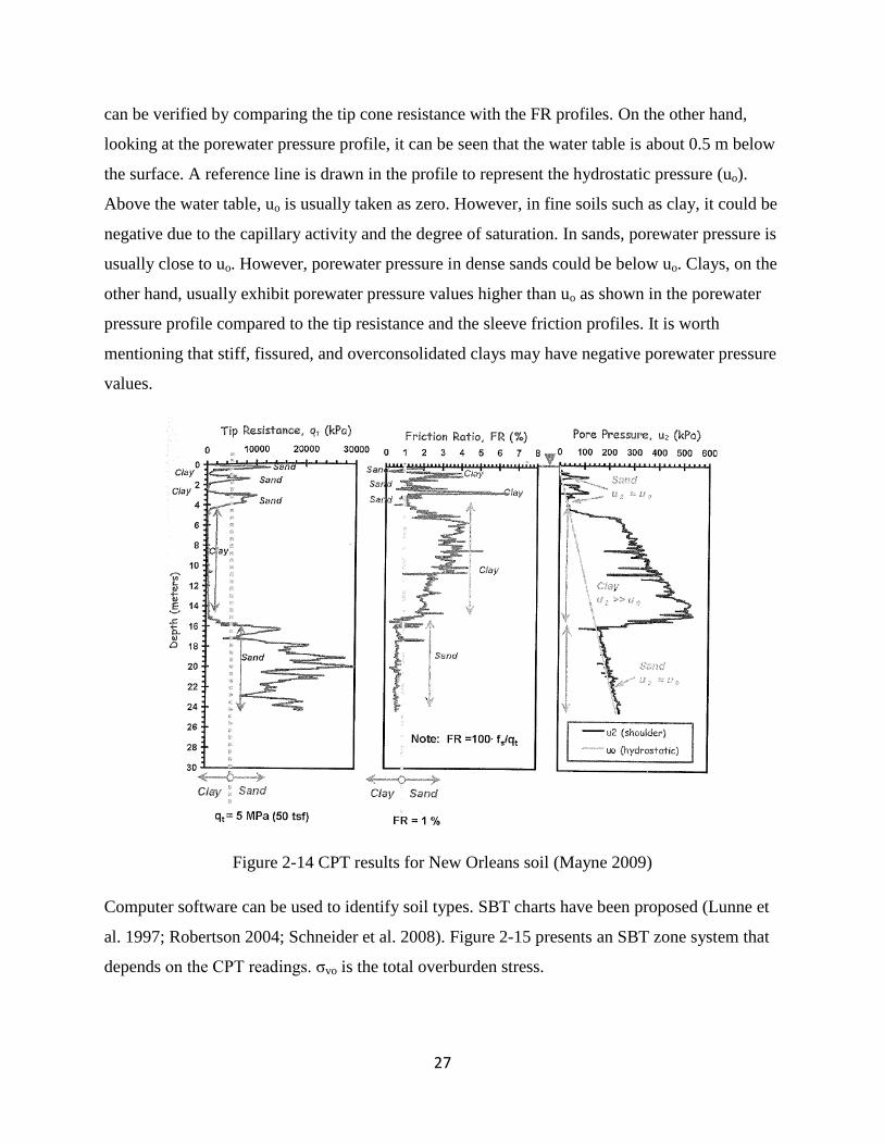
27
can be verified by comparing the tip cone resistance with the FR profiles. On the other hand,
looking at the porewater pressure profile, it can be seen that the water table is about 0.5 m below
the surface. A reference line is drawn in the profile to represent the hydrostatic pressure (uo).
Above the water table, uo is usually taken as zero. However, in fine soils such as clay, it could be
negative due to the capillary activity and the degree of saturation. In sands, porewater pressure is
usually close to uo. However, porewater pressure in dense sands could be below uo. Clays, on the
other hand, usually exhibit porewater pressure values higher than uo as shown in the porewater
pressure profile compared to the tip resistance and the sleeve friction profiles. It is worth
mentioning that stiff, fissured, and overconsolidated clays may have negative porewater pressure
values.
Figure 2-14 CPT results for New Orleans soil (Mayne 2009)
Computer software can be used to identify soil types. SBT charts have been proposed (Lunne et
al. 1997; Robertson 2004; Schneider et al. 2008). Figure 2-15 presents an SBT zone system that
depends on the CPT readings. σvo is the total overburden stress.

28
Figure 2-15 Soil identification by using soil behavior type (Lunne et al. 1997)
2.2.3 Background on ball penetrometers
The initial idea of a ball penetrometer was taken from a miniature T-bar that was used in
centrifugation (Boylan et al. 2011). Later, full flow penetrometers were used to improve
resistance by increasing the tip projected area (Stewart and Randolph 2001). Then, full flow
penetrometers were used on offshore soils as they are a soft type of soil (Randolph et al. 1998).
Ball penetrometers which were introduced as the tip of T-bar penetrometers may bend as they
are driven into the ground (Watson et al. 1998). The main advantage of full flow penetrometers
over conventional cone penetrometers is the increase in the projected area. This increase in the
projected area reduces the effects of temperature and overburden stress as the soil would flow
around the ball or T-bar tip instead of being displaced as in the case of a cone tip (Boylan et al.
2011).

29
2.2.3.1 Penetration Resistance Correction
The tip resistance of ball penetrometers needs to be corrected for pore water pressure and
overburden stress that do not act on top of the ball because of the push rods, as soil does not flow
but displaces around them (Randolph 2004; Randolph et al. 2007; DeJong et al. 2009, 2010 and
2011; Low et al. 2010; Boylan et al. 2011):
2[ (1 )] sball m v
p
Aq q u a
A
where qball is the corrected tip resistance, qm is the measured tip resistance, σv is the total
overburden pressure, a is the area ratio obtained in accordance with ASTM D 5778, As is the
projected area of the push rods, and Ap is the projected area of the tip. DeJong et al. (2010)
suggested the use of hydrostatic pore water pressure for unmeasured pore water pressure during
testing in the field. However, porewater pressure at Position 2 (u2) is measured for all of the
penetrometers in this study.
2.2.3.2 Undrained Shear Strength
Undrained shear strength (su) can be obtained by field vane or laboratory testing. The following
formula is suggested which uses Nsu as a strength factor (Randolph 2004; Randolph et al. 2007;
DeJong et al. 2009, 2010 and 2011; Boylan et al. 2011; Low et al. 2010):
ballu
Su
qs
N
Studies have shown that sensitivity and rate of penetration may affect the calculation of NSu
(DeJong et al. 2008 and 2009).
2.3 Correlations from the Canadian Foundation Engineering Manual
Table 2-1 is taken from Table 3.3 in the Canadian Foundation Engineering Manual. This table
correlates the undrained shear strength of clays to N60 values from standard penetration testing.
Table 2-2 is taken from Table 6.1A in the same manual. This table correlates the shear wave
velocity from downhole seismic testing and undrained shear strength (from vane tests for
example) to site class.

30
Table 2-1 Table 3.3 in the Canadian Foundation Engineering Manual (2005)
Consistency Undrained Shear Strength (kPa) SPT N-Index (blows/0.3m)
Very Soft <12 <2
Soft 12-25 2-4
Firm 25-50 4-8
Stiff 50-100 8-15
Very Stiff 100-200 15-30
Hard >200 >30
Table 2-2. Table 6.1A in the Canadian Foundation Engineering Manual (2005)
Site Class Soil Profile Name
Average Properties in Top 30 m as per Appendix A NBCC 2005
Soil Shear Wave Average Velocity
(m/s)
Standard Penetration
Resistance N60
Soil Undrained Shear Strength Su
A Hard Rock Vs>1500 Not applicable Not applicable
B Rock 760<Vs<1500 Not applicable Not applicable
C Very Dense Soil and Soft Rock
360<Vs<760 N60 > 50 Su > 100 kPa
D Stiff Soil 180<Vs<360 15 <= N60 <= 50 50 kPa <= Su <= 100
kPa
E Soft Soil Vs<180 N60 <15 Su < 50 kPa
E Any profile with more than 3 m of soil with the following characteristics:

31
Plastic index >20
Moisture content >= 40%, and
Undrained shear strength < 25 kPa
F Others Site specific evaluation required
Other correlations between penetrometers, and other laboratory and field testing, and engineering
characteristics of sensitive marine clays, are briefly reviewed in Technical Papers I and II.
Therefore, they will not be reviewed here to avoid repetition.
2.4 Summary and Conclusion
Sensitive marine clay is mainly the product of proglacial and post glacial sedimentation after the
advancement of the Wisconsin Ice Sheet. Postglacial depositions of Ottawa sensitive marine
clays are predominantly done so by the Champlain Sea which covered Ottawa from 12500 to
10000 years BP.
As a result of proglacial and postglacial deposition, varved marine clays formed. A layer of one
year of deposition consists of the silt (80% >2 µm) and clay (80% <2 µm) layers, and the
transition layer in between.
The main minerals of the Ottawa clays are quartz, feldspar, amphibole, mica, chlorite, smectite,
and glacial amorphous material. Carbonates may also be present in these clays. Three main types
of sedimentation processes in general, are responsible for marine clays in Canada, which are
waterlaid tills, lacustrotills, and mudflows.
Salinity and other cations, such as Na, K, Ca, and Mg, affect the behavior and sensitivity of
marine clays. A double layer of marine clay particles also affect the behavior of these clays.
Penetrometers are increasingly being used in marine clays. Correlations have been established by
researchers to relate the outcomes of penetrometer testing and the engineering characteristics of
these clays.
The behaviour of sensitive marine clays in Ottawa is still not well understood. Readings by cone
and ball penetrometers are significantly affected by temperature changes. The rate of rotation for

32
the field vanes may not be adequate to estimate the remolded shear strength of these clays.
Laboratory vane results may misestimate the shear strength of these clays when compared to that
of field vanes. Also, from the results of this research, the Canadian Foundation Engineering
Manual may have underestimated the undrained shear strength of sensitive marine clays in
Ottawa. These are the reasons that this research has been conducted.
2.5 References
Aber, J. S. (2005). Glacial Geology of the Kansas City Vicinty. U.S. Forest Service. Retrieved 7
8, 2013, from http://www.geospectra.net/lewis_cl/geology/glacial.htm
Almeida, M. S. S., Danziger, F. A. B, Lunne, T. (1996). Use of piezocone test to predict the axial
capacity of driven and jacked piles in clay. Canadian Geotechnical journal, 33(1):33-41.
Andrews, J. T. (1972). The National Atlas of Canada. Canada Department of Energy, Mines and
Resources.
Andrews, J. T. (1986). The pattern and interpretation of restrained, post-glacial and residual
rebound in the area of Hudson Bay. Geological Survey of Canada Paper 49-62.
Andrews, J. T., Peltier, W. R. (1976). Collapse of the Hudson Bay ice centre and glacio-isostatic
rebound. Geology 4:73-75.
ASTM D 4318 (2005). Standard Test Methods forLiquid limit, Plastic limit, and Plasticity Index
of soils.
Ballivy, G., Loiselle, A. A., Pouliot, G. (1975). Quelques caractkristiques gkotechniques des
d'pBts d'argile de la baie James: les coulCes d'argile de Fort Rupert, Quebec. Canadian
Geotechnical Journal 12:498-509.
Ballivy, G., Pouliot, G., Loiselle, A. (1971). Quelques caracteristiques geologique et
mineralogiques des depots d'argile du nord-ouest du Quebec. Canadian Journal of Earth
Science 8:1525-1541.
Bentley, S. P., Smalley, I. J. (1979). MINERALOGY OF A LEDA/CHAMPLAIN CLAY FROM
GLOUCESTER. Engineering Geology 14:209-217.

33
Bentley, S. P., Smalley, I. J. (1978). Mineralogy of sensitive clays from Quebec. Canadian
Mineralogist 16:103-112.
BERRY, R. W. (1988). Mineralogy, grain size distribution and geotechnical behavior. The C
anndian Mineralogist 36:1625-1636.
Boissonneau, A. (1966). Glacial history of northeastern Ontario: I. The Cochrane-Hearst area.
Canadian Journal of Earth Sciences 3:559-578.
Briaud, J.-L. (2007). Spread foorings in sand: Load-settlement curve approach. Journal of
Geotechnical and Geoenvironmental Engineering 133(8):905-920.
Brydon, J. E., Patry, L. M. (1961). Mineralogy of Champalin Sea sediments and a Rideau clay
soil profile. Canadian Journal of soil science 41:169-181.
Cronin, T. M. (1977). Late-Wisconsin marine environments of the Champlain Valley (New York,
Quebec). Quaternary Research 7:238-253.
Demers, D. L. (2002). Evaluation of preconsolidation pressure and the overconsolidation ratio
from piezocone tests of clay deposits in Quebec. Canadian Geotechnical Journal 39(1):174-192.
Dreimanis, A. (1976). Tills: Their origin and properties. Royal society of Canada Special
Publication 12:11-49.
Dreimanis, A. (1977). Correlation of Wisconsin glacial events between the eastern Great Lakes
and the St. Lawrence Lowlands. Gkographie, Physique et Quaternaire 37-51.
Dreimanis, A. (1977). Late Wisconsin glacial retreat in the Great Lakes region, North America.
Annals of the New York Academy of Sciences 288:70-89.
Elson, J. A. (1967). Geology of glacial Lake Agassiz. University of Manitoba Press 36-95.
Fall, M. (2011). Geotechnical Hazards. The University of Ottawa, Ottawa.
Fanning, D.S., Jackson, M.L. (1966). Clay mineral weathering in southern Wisconsin soils
developed in loess and in shale-derived till. Proceedings, 13th Conference 175-191.
Gadd, N. R. (1975). Geology of Leda clay. Geo Abstracts Ltd 137-151.

34
Gillott, J. E. (1971). Mineralogy of Leda clay. Canadian Mineralogist 10:797-811.
Group, N. P. (June 4 1971). Nature of Quickclays. Nature 231.
Hendershot, W. H., Carson, M. A. (1978). Changes in the plasticity of a sample of Champlain
clay after selective chemical dissolution to remove amorphous material. Canadian Geotechnical
Journal 15:609-616.
Hillaire-Marcel, M. C. (Published these de Doctorat d'Etat ks Sciences Naturelles, Universitk
Pierre et Marie Curie, Paris). 1979. Les nlers post-glaciaires du Quebec: quelques aspects 2.
Houston, W. N., Mitchell, J. K. (1969). Property interrelationships in sensitive clays. ASCE
Journal of the Soil Mechanics and Foundation Division, 95:1037-1062.
Jones, G. A., Van Zyl, D. J. A. (1981). The piezometer probe: a useful invertigation tool. 10th
internation conference of soil mechanics and foundation engineering 3:489-495.
Kenney, T. (1976). Formation and geotechnical characteristics of glacial-lake varved soils.
Norwegian Geotechnical Institute Publication 15-39.
Konrad, K., & Law, J. (1987). Undrained shear strength from piezocone tests. Canadian
Geotechnical Journal 24:392-405.
Kulhawy, F. H., Mayne, P. W. (1993). Drilled shaft side resistance in clay soil to rock. design
and performance of deep foundation 172-183.
La Rochelle, P., Lefebvre, G. (1971a). Sampling disturbance in Champlain clays. American
society for testing and materials 483:143-163.
Lee, K. L. (1979). Cyclic strength of a sensitive clay of eastern Canada. Canadian Geotechnical
Journal 16:163-176.
Leroueil, S. (1999). Geotechnical characteristics of eastern Canada clays. Characteristics of
Soft Marine Clays, ISBN 90 5809 104X.
Letoueil, S., Tavenas, F., Le Bihan, J. P. (1983a). Proprietes caracteristiques des argiles de l'est
du Canada. Canadian Geotechnical journal 20(4):681-705.

35
Lo, K. Y., Ho, K. S. (1991). The effects of electroosmotic field treatment on the soil properties of
a soft sensitive clay. Canadian Geotechnical Journal 28:763-770.
Locat, E. D. (1996). O n the developmenot f microstructurein. In Genesis and Properties of
Collapsible 93-128.
Lunne, T., Robertson, P. K., Powell, J. J. M. (1997). Cone Penetration Testing in Geotechnical
Practise. Blackie Academic, New York.
May, R. (1977). Facies model for sedimentation in the glaciolacustrine environment. Boreas
6:175-180.
Mayne, P. W. (2009). Engineering Design Using the Cone Penetration Test-Geotechnical
Application Guide. ConeTec, USA.
Mayne, P. W., Kulhawy, F. H. (1982). Ko-OCR relationship in soils. Journal of Geotechnical
Engineering 106:851-872.
Mayne, P. W., Stewart, H. E. (1988). Pore pressure response of K-consolidated clays. Journal of
Geotechnical Engineering 114(11):1340-1346.
Morgenstem, N. (1967). Submarine slumping and the initiation of turbidity currents. University
of Illinois Press 189-220.
Nagaraj, T. S., Murthy, B. R. S., Vatsala, A., Joshi, R. C. (1990). Analysis of compressibility of
sensitive soils. Journal of Geotechnical Engineering 116(1):105–118.
Nishimura, T., Hirabayashi, Y. Fredlund, D. G., Gan, J. K. M. (1999). Influence of stress history
on the strength parameters of an unsaturated statically compacted soil. Canadian Geotechnical
Journal 36:251-261.
Peck, R. B., Ireland, H. O., Fry, T. S. (1951). U illinois civ. Eng. Dep. soil Mech. series 1.
Penner, E. (1965). A study of the sensitivity of Leda clay. Canadian Journal of Earth Sciences 2.
Penner, E. (1970). Frost heaving forces in Leda Clay1. Canadian Geotechnical Journal 7:8.

36
Poulus, H. G., Davis, E. E. (1974). Elastic solutions for soil and rock mechanics. John Wiley and
sons Inc. 213.
Push, R., Arnold, M. (1969). Engineering Geology 3:135.
Quigley R.M., T. (1976). Till geology, mineralogy and geotechnical behaviour, Sarnia, Ontario.
Royal Society of Canada Special Publication 12:336-345.
Quigley, R. M. (1980). Geology, mineralogy, and geochemistry of Canadian soft soils: a
geotechnical perspective. Canadian Geotechnical Journal 17:261-285.
Robertson, P. K. (1990). Soil classification using the cone penetration test. Canadian
Geotechnical Journal 27:151-158.
Robertson, P. K. (2004). Evaluating soil liquifaction and post-earthquake defor-mations using
the CPT Geotechnical and Geophysical Site Characteristics. Millpress, Rotterdam 1:233-249.
Roy, M., Blanchet, R., Tavenas, F., La Rochelle, P. (1981). Behaviour of a sensitive clay during
pile driving. Canadian Geotechnical Journal 18:67-85.
Saihi, F., Leroueil, S., La Rochelle, P., French, I. (2002). Behaviour of the stiff and sensitive
saint-jean-vianney clay in intact, destructed, and remoulded conditions. Canadian Geotechnical
Journal 39:1075–1087.
Senneset, K., Sandven, R., Lunne, T., Amundsen, T. (1988). Piezocone tests in silty soils.
Proc.ISOPT-Orlando 2:955-974.
Simon, G., Hache, R., Fred, J. G. (2010). Esprit Drive Overpass-Cumberland Transitway.
Stantec Consulting Ltd, Ottawa.
Simon, G., Hache, R., Fred, J. G. (Dec 2010). Portbello Boulevard Overpass-Cumberlan
Transitway Project. Stantec Consulting Ltd, Ottawa.
Smith, N. (1978). Sedimentation processes and patterns in a glacier-fed lake with low sediment
input. Canadian Geotechnical Journal 15:741-756.

37
Soderman, L. G., Quigley, R. M. (1965). Geotechnical properties of three Ontario clays.
Canadian Geotechnical Jounal 2:167-189.
Syvitski, J. (1980). Flocculation, agglomeration and zooplankton pelletization of suspended
sedinient in a fjord receiving glacial meltwater. In Fjord oceanography, NATO Conference
4:616-625.
Syvitski, J. P. (1978). Sedimentological advances concerning the flocculation and zooplankton
pelletization of suspended sediment in Howe Sound, British Columbia: A fjord receiving glacial
meltwater. Ph.D. thesis, University of British Columbia, British Columbia, Vancouver, B.C.
Syvitski, J. P., Murray, J. W. (1980). Particle interaction in fjord suspended sediment. Marine
Geology, In Press.
Tavenas, F., Tremblay, M., Larouche, G., Leroueil, S. (1986). In situ measurement of
permeability in soft clays. ASCE Special Conference 1034-1048.
Tevanas, F., Leroueil, S. (1987). State-of-the-art on laboratory and in-situ stress-strain-time
behaviour of soft clays. International Symposium on Geotechnical Engineering of soft soils 1-
146.
Torrance. (1988). Mineralogy, pore-water chemistry, and. In The late Quaternary Development
35:259-275.
Torrance, J. K. (1979). Post-depositional changes in the pore water chemistry of the sensitive
marine clays of the Ottawa area, eastern Canada. Canada Engineering Geology 14:135-147.
Walker, L. K., Raymond, G. P. (1966). The prediction of consolidation rates. Canadian
Geotechnical Journal 4.
Walker, L. K., Raymond, G. P. (1969). Anisotropic consolidation of Leda clay. Canadian
Geotechnical Journal 6:271.
Yafrate, N., & DeJong, J. (2006). Interpretation of sensitivity and remolded undrained shear
strength with full flow penetrometers. Davis, CA, USA.

38
Yong, R. N., Sethi, A. J., La Rochelle, P. (1979). significance of amorphous material relative to
sensitivity in some Champlain clays. Canadian Geotechnical Journal 16:511-520.
Yong, R. N., Silvestri, V. (1979). Anisotropic behaviour of a sensitive clay. Canadian
Geotechnical Journal 16:335-350.
Battaglio, M., Jamiolkowsi, M., Lancellotta, R., Maniscalco, R. (1981). Piezometer probe test in
cohesive deposits. Proceedings of the Session ASCE National Convention, (pp. 264-302). St.
Louis.
Lunne, T., Robertson, P., Powell, J. (1997). Cone Penetration Testing. Blackie Academic &
Professional.
Randolph, M., Wroth, C. (1979). An analytical solution for the consolidation around a driven
pile. Proceedings of the International Journal for Numerical and Analytical methods in
Geotechnics, (pp. 217-29).
Massarsch, K., Broms, B. (1981). Pile driving in clay slopes. Proceedings of the 10th
International Conference on Soil Mechanics and Foundation Engineering (pp. 469-74).
Stockholm: Balkema Pub.
Campanella, R., Robertson, P., Gillespie, D., Greig, J. (1985). Recent developments in in-situ
testing of soils. Proceedings of the 11th International Conference on Soil Mechanics and
Foundation Engineering (pp. 849-54). San Francisco: Balkema Pub.
Schmertman, J. (1978). Guidelines for cone penetration test, performance and design.
Washingto, DC: US Federal Highway Administration.
Robertson, P., Campanella, R. (1983). Interpretation of cone penetration test. Canadian
Geotechnical Journal , 20(4), 734-45.
Robertson, P., Campanella, R., Gillespie, D., Greig, J. (1986). Use of piezometer cone data.
Proceedings of the ASCE Specialty Conference In Situ '86: Use of In Situ tests in Geotechnical
Engineering (pp. 1263-80). Blacksburg: ASCE.

39
Robertson, P. (1990). Soil classification using the cone penetration test. Canadian Geotechnical
Journal , 27(1), 151-8.
Kulhawy, F., Mayne, P. (1990). Manual on estimating soil properties for foundation design.
Electrical Power Research Institute.
Jefferies, M., Davies, M. (1991). Soil classification by the cone penetration test. Canadian
Geotechnical Journal , 28(1), 173-6.
Suzuki, Y., Tokimatsu, K., Kubota, Y. (1995). Correlation between CPT data and dynamic
properties of in situ frozen samples. Proceedings of the Third International Conference on
Recent Andances in Geotechnical Earthquake Engineering and Soil Dynamics (pp. 249-52). St.
Louis: University of Missouri Rolla.
Stewart, D., Randolph, M. (2001). A new site investigation tool for the centrifuge. Proceedings of
the International Conference Modelling (pp. 531-538). The Netherlands: Balkema.
Randolph, F., Hefer, P. A., Geise, J. M., Watson, P. (1998). Improved seabed strength using T-
bar penetrometer. Proceedings of the International Conference on Offshore Site Investigation
and Foundation Behaviour (pp. 221-235). London: Society for Underwater Technology.
Randolph, M. (2004). Characterization of soft sediments for offshore applications. ISC-2 on
Geotechnical and Geophysical Site Characterization (pp. 209-232). The Netherlands: Millpress.
Randolph, M., Low, H., Zhou, H. (2007). In situ testing for design of pipeline and anchoring
systems. Proceedings of the Sixth International Conference on Offshore Site Investigation and
Geotechnics (pp. 251-262). London: Society for Underwater Technology.
Watson, P., Newson, T., Randolph, M. (1998). Strength profiling in soft offshore soils. In
Proceedings of the 1st International Conference on Site Characterisation (pp. 1389-1394).
Atlanta: Edited by Robertson, P.K., Mayne, A.A. Balkema, Rotterdam, the Netherlands .
Boylan, N., Long, M., Mathijssen, F. (2011). In situ strength characterization of peat and
organic soil using full-flow penetrometers. Canadian Geotechnical Journal , 48: 1085-1099.

40
Low, H., Lunne, K., Andersen, M., Li, X., Randolph, M. (2010). Estimation of intact undrained
shear strength from penetration tests in soft clays. Geotechnique , 11, 843-859.
DeJong, J. T., Yafrate, N. J., DeGroot, D. J. (2011). Evaluation of undrained shear strength
using full-flow penetrometers. Journal of geotechncial and Geological Engineering , 14-26.
DeJong, J., DeGroot, D., Randolph, M. (2009). Evaluation of shear strength and sensitivity of
soft clay using full-flow penetrometers. Journal of Geotechnical and Geological Engineering ,
1179-1189.
DeJong, J., Yafrate, N., Randolph, M. (2008). Use of pore pressure measurements in a ball full
flow penetrometer. Geotechnical and Geophysical Site Characterization (pp. 1269-1275).
Taipei: Taylor and Francis.
DeJong, J., Yafrate, N., DeGroot, D., Low, H. E., Randolph, M. (2010). Recommended practice
for full-flow penetrometer testing and analysis. Geotechnical Testing Journal , Vol. 33, No. 2.

41
Chapter 3: Technical Paper I - Geotechnical Properties of Sensitive
Marine Clays - Examples of Clays in Eastern Canada
N.Athir, M. Fall, R. Hache
Abstract
This article presents a comprehensive description and review of the geotechnical properties of
sensitive marine clays in the Canadian capital region. The general behaviour of these clays is
discussed which provides the engineers who work with these clays with a better understanding of
the geotechnical properties of sensitive marine clays in eastern Canada. Fifteen sites are taken
into consideration. Geotechnical investigations have been carried out in these sites. These
geotechnical investigations included cone and standard penetration tests, split spoon and
undisturbed sampling, field vanes, and shear wave velocity measurements. Laboratory tests are
also carried out on the samples. These laboratory tests include consolidation testing,
determination of grain size distribution, porewater chemistry analysis, and determination of
physical and index properties. This research compares these results with available data from
other research along with other characteristics, such as sensitivity, activity, interface shear
strength, and hydraulic conductivity, depending on the availability of data from each site.
It is found that the Canadian Foundation Engineering Manual may have underestimated the
undrained shear strength of these clays. The moisture contents of these clays are close to or
exceed the liquid limits which may contribute to the sensitive behaviour of sensitive marine clays
in Ottawa. The activities of these clays fall in the normal and inactive areas of the activity chart.
The ratio of the secondary compression index to the compression index presented in the literature
for marine clays in Canada may not be applicable for sensitive marine clays in Ottawa. It is also
discussed that laboratory vanes may have overestimated or underestimated the undrained shear
strength compared to field vanes. A wide range of soil specific cone factors is also presented in
this research.

42
Keywords
Engineering characteristics, Laboratory testing, In-Situ, Gloucester, Ottawa, Leda Clay,
Sensitive Marine Clay
3.1 Introduction
Marine clays cover large areas in the world, such as Canada, Norway, Sweden, Scandinavia, and
Russia. In Canada, marine clays cover large areas in the provinces of Ontario and Quebec. These
clays are commonly called Leda clays in Ontario and Champlain Sea clays in Quebec. The soft
consistency and sensitive behavior of these clays make them challenging to geotechnical
engineers. These clays can change from a solid to liquid consistency only by disturbance which
makes them prone to landslides and foundation damage.
It is important to increase local experience on the behavior and engineering characteristics of
marine clays. There is a demand for local experience as a result of the infrastructure expansion in
the capital region. Many researchers have examined the engineering characteristics of marine
deposits in the Canadian capital region. However, there has not been an attempt to collect and
analyse the available data for reference. Consequently, this is the reason for the initiation of this
research.
Marine deposits in Ottawa exhibit unique behaviour that is different from similar deposits in
different parts of the world or even different parts of Canada. Therefore, the correlations that are
made on similar marine deposits should be examined and verified for marine deposits in Ottawa.
Fifteen sites have been selected from the Canadian capital region. These sites were originally
investigated for geotechnical design purposes. Field investigations and laboratory tests are
carried out on the sites and samples obtained from them. The field tests include cone and
standard penetration testing, split spoon and undisturbed sampling, and field vanes and
monitoring well testing. Laboratory tests include testing of consolidation, grain size distribution,
porewater chemistry, specific gravity, plasticity, moisture content, and unit weight. This research
compares the outcomes of field and laboratory tests with previously reported results. The work
analyzes plasticity, activity, sensitivity, hydraulic properties, shear strength behaviour and
interface, and physical characteristics. It also reports on the outcomes of the cone and standard

43
penetration tests, and vane tests. The study reports the values of the consolidation history of the
soil obtained from the site under study including Canadian Geotechnical Research Site No. 1 (or
Site 6 as named in this research). This research also discusses the underestimation of the shear
strength of sensitive marine clays in Ottawa by the Canadian Foundation Engineering Manual.
This paper is organized as follows: first, the geographical and geological characteristics of the
area under study are discussed. Second, the physical characteristics, Atterberg limits, and activity
of sensitive marine clays in Ottawa are examined. Then, the geotechnical in-situ testing is
presented. This is followed by an outline of the shear strength and deformation behaviour. After
that, the interface shear strength and behaviour are discussed. Then, the consolidation behaviour
is presented, followed by a discussion on the sensitivity of marine clays in Ottawa. Finally, the
permeability will be examined.
3.2 Geographical and Geological Characteristics
3.2.1 The Sites
Fifteen sites (Sites 1 to 15) are selected for this study. The locations of the sites are shown in
Figure 3-1. The sites are well spread out on the most developed areas in Ottawa which allow for
a rather comprehensive study of the marine deposits in the region. All of the site stratifications
from the geodetic surface elevation to the bedrock are shown in Figure 3-2. However, no
dimensions are given for Sites 14 and 15, but the stratification on these two sites from the surface
to the bedrock are as follows: silty sand to sand and gravel fill with traces of organics in some
areas of the sites, clay with 0.9 m of crust (0% to 1% gravel, 2% to 11% sand, 18% to 26% silt,
62% to 80% clay), and till or silty sand with gravel and traces of cobbles and boulders (10% to
22% gravel, 39% to 48% sand, 30% to 51% silt and clay). Bedrock is found at depths of 2.1 to
7.6 m. The sites have geodetic elevations of 66.4 m to 71.5 m and water table depths of 2.9 to 4.7
m. These results in terms of the stratification are consistent with those obtained by Eden and
Crawford (1957), who made five boreholes that are well spread over Ottawa.

44
Figure 3-1 Location map of sites obtained from Google Earth

45
(a) (b)
(c) (d)
-3.2
6.8
16.8
26.8
36.8
46.8
56.8 G
eo
deti
c E
levati
on
[m
] water table
Granular fill
Organic top soil (0.1 m)
Silty sand (70% sand and 30% silt)
Silty clay (11% to 20% silt and 80% to 89% clay)
Glacial till deposit (0% to 16% gravel, 24% to 92% sand, and 8% to 76% silt and clay) 59.5
64.5
69.5
74.5
79.5
84.5
89.5
Geo
de
tic E
levati
on
[m
]
Fill (silty sand to silty gravel)
Organic top soil (0.15 m)
Clay with 3 m of fat clay crust (20% sand, 25% silt, and 55% clay) and lean clay (7% to 40% sand, 36% to 78% silt, and 15% to 45% clay)
Glacial till (44% gravel, 48% sand, and 8% silt)
Water table
63.8
68.8
73.8
78.8
83.8
88.8
Geo
de
tic E
levati
on
[m
]
water table
Sand
Organic top soil (0.15 m)
Clay with 3.6 m of fat clay crust and lean clay
Till (gravel, sand, silt)
43.4
48.4
53.4
58.4
63.4
68.4
Geo
de
tic E
levati
on
[m
]
water table
Silty clay with sand and gravel
Organic top soil (0.1 m)
Silty sand
Clay
Till (silty sand with traces of gravel, cobbles, and boulders )
Gravelly sand

46
(e) (f)
(g) (h)
33.8
38.8
43.8
48.8
53.8
58.8
63.8
68.8
Geo
de
tic E
levati
on
[m
] water table
Sandy silt to silty sand
Organic top soil or silty clay (0.15 m)
Clay with 3 m of fat clay crust and lean clay
Glacial till (silty sand with gravel)
58.4
63.4
68.4
73.4
78.4
Geo
de
tic E
levati
on
[m
]
water table
Sand and silt
Organic top soil (0.3 m)
Silty clay
Clay
Varved clay and silt
Silty clay
Clay, silt, sand, and gravel
72.8
77.8
82.8
87.8
92.8
97.8
Geo
de
tic E
levati
on
[m
]
water table
Clay with 5.3 m of crust (46% silt and 54% clay)
Fill (0.6 m of sand and gravel)
Sandy silt with traces of gravel (45% sand, 26% silt, and 16% clay)
Glacial till (gravel, sand, silt)
38.3
40.3
42.3
44.3
46.3
48.3
50.3
52.3
Geo
de
tic E
levati
on
[m
]
Clayey sand to sandy gravel with cobbles and boulders (17% to 23% gravel, 36% to 50% sand, and 27% to 47% silt and clay)
Organic top soil (0.2 m)
Clay with 1.6 m crust (46% silt and 54% clay)
Glacial till (silty sand)
Water table

47
(i) (j)
(k) (l)
69.5
74.5
79.5
84.5
89.5
94.5
99.5 G
eo
deti
c E
levati
on
[m
] water table
Clay with 2.6 m of crust
Fill (0.6 m of silty sand and gravel)
Till (sandy silt)
78.2
80.2
82.2
84.2
86.2
88.2
90.2
Geo
de
tic E
levati
on
[m
]
water table
Silty clay with traces of sand, gravel, and organics
Organic top soil (0.1 m)
Clay with 1.5 m of crust
Till (silty sand with gravel and traces of cobbles and boulders)
53
58
63
68
73
78
83
88
Geo
de
tic E
levati
on
[m
]
water table
Clay with gravel
Organic top soil (0.1 m)
Clay with 2.7 m of crust
Till (silty sand with gravel and traces of cobbles and boulders)
79
80
81
82
83
84
85
86
87
88
89 G
eo
de
tic E
levati
on
[m
] water table
Fill (silty clay with gravel)
Organic top soil (0.1 m)
Clay
Till (silty sand with gravel and traces of cobbles and boulders)

48
(m)
Figure 3-2 Stratification for (a) Site 1 (b) Site 2 (c) Site 3 (d) Site 4 (e) Site 5 (f) Site 6 (g) Site 7
(h) Site 8 (i) Site 9 (j) Site 10 (k) Site 11 (l) Site 12 (m) Site 13
3.2.2 Origin and Geological Setting
Quigley (1980) mentioned that soils in Canada are the products of sedimentation in proglacial
and postglacial water bodies that existed during the retreat of the Wisconsin Ice Sheet between
18 000 and 6000 years before presence (BP). The retreat of the ice sheet happened in stages and
then stopped in some periods. The retreat was accompanied by glacial lakes that existed at the
ice front and seas in the lowlands. The Champlain Sea covered Ottawa between 12500 and
10000 BP as a result of ice front retreat and re-advance, and was "expelled" as result of "crustal
rebound" (Cronin, 1977; Elson, 1967; Gadd, 1975; Hillaire-Marcel, 1979). A rebound of 200 m
is estimated for Ottawa. Ice front readvances in 13500, 11800, and 8200 years BP are believed to
have deposited soft clays during those periods of time. The formation of glacial lakes and seas
are affected by the volume of water supplied by the ice melt, rate of crustal rebound, and
existence of outlets from one water body to another. The Champlain Sea is believed to have
covered Ottawa after the melt down of the ice dam near Quebec City (Gadd 1975). An ice front
is considered to have bordered the northern side of the sea for hundreds of years. Deposits close
to the centre of the Champlain Sea are thick clay deposits while those away from the centre are
clay interlayered with fluvial sand and gravel or glacial till.
68.8
73.8
78.8
83.8
88.8
Geo
de
tic E
levati
on
[m
]
water table
Fill (clay with gravel)
Organic top soil (0.1 m)
Clay with 2.8 to 4. 3 m of crust
Till (silty sand with gravel and traces of cobbles and boulders)

49
Gadd (1975) divided deposits according to their origin into five types: waterlaid tills,
lacustrotills, mudflow deposits, turbidity current deposits, and varved and marine clays.
Waterlaid till is believed to be lacustrine clay deposited below shallow ice sheets with minimum
particle gradation in a study performed by May (1977) on Alberta clays. Waterlaid till is usually
underlain by hard till. In the same study, lacustrotills are indicated as soft till soils deposited by
submarine mud flows in glacial lakes. Lacustrotills may contain waterlaid tills as they are
deposited by turbidity currents. Depending on the rate of acceleration of the mud flow,
lacustrotills may interlay with clay deposits (Morgenstern, 1967). The term "varved clays"
denotes deposits in layers of summer silt and winter clay in glacial freshwater lakes. Varved clay
sediments in proglacial clays are controlled by sediment concentration in the inlet flow. In the
summer, a cold water flow of 1 g/L or more of sediment concentration enters the lake. This flow
is higher in density than the lake which results in submarine flow that can run for miles, thus
depositing a layer of silt and sand. In the winter, the inflow is low in sediments, which results in
overflow in the lake, thus resulting in slow sedimentation of clay particles (Kenney et al. 1976).
In postglacial lakes, sediment concentration is reduced to less than 0.1 g/L. Therefore, there were
overflow and inflow rather than submarine flow and the deposits became controlled by "thermal-
density stratifications". As a result of the reduced sediment concentrations and underflow,
couplets are clearly found near the outlet, but summer deposits became thin away from the
outlets.
Summer deposits contain less than 80% passing 2 µm while winter deposits contain more than
80% passing 2 µm (Chan and Kenney, 1973). There are also transition layers in between. In
general, higher moisture contents, and liquid and plastic limits are observed for couplets in the
winter as opposed to the summer. A high moisture content of 75% indicates an "open flocculated
structure"(Quigley and Ogunbadejo, 1972). A schematic figure by Quigley (1980) shows that the
coarser couplet in the summer is thicker than the clay layer in the winter and can be up to 1 m in
thickness. Due to depositions in salt or sea water, freshwater inlets would enter the sea as
overflows as a result of the high density of the sea water from high salinity concentration. Sea
water has a salinity concentration of 30%, primarily of sodium chloride (NaCl) with a density of
1020 g/L while the concentration of salinity in freshwater can be up to 4 g/L. Therefore,
subglacial flows would rise to the surface and there would be little turbidity current activity
(Quigley, 1980). Ottawa lands had a crustal rebound of about 200 m (Andrews, 1972). The

50
Champlain Sea was very deep in its early stages (Kenney, 1964). The Sea had a salinity of
approximately 35 g/L. When freshwater from ice front melting or inlets enter the seawater or salt
water, it is mixed by diffusion and turbulence in the first 5 m of the surface layer of the sea. In
the same layer, clay particle flocculation begins. Below this layer, pelletization (biological
activities) affects the clay floccules (Syvirski, 1978; Syviski and Murray, 1980; Syvitski et al.
1980). These clay floccules contain organic matter and siliceous and calcareous shell fragments.
"Black mottling" common in marine clays is attributed to bacterial activity in organic matter. The
organic matter is reported to be between 0.4% to 1% (Donovan and Lajoie, 1979; Laventure and
Warkentin, 1965).
3.2.3 Porewater Chemistry
A porewater chemistry analysis was performed by Haynes and Quigley (1978) on sensitive
marine clay in Hawkesbury about 90 km to the east of Ottawa. The study was also mentioned by
Taha et al. (2010). The clays primarily contain sodium (Na+) with magnesium (Mg
2+), calcium
(Ca2+
) and potassium (K+) ions. The salinity ranges from 2 g/L at the surface to 15 g/L at a depth
of 30 m.
Taha et al. (2010) reported NaCl concentration of 3 to 4 g/l in their marine clay samples from
Ottawa. Dayal (1970) reported salt content from other research work, such as that by Crawford
(1961), Crawford (1968), and Crawford and Eden (1965), for sensitive marine clays to be
between 0.3 to 15 g/l.
Sulphate, chloride, pH, and resistivity have been analyzed for a few samples from the sites
studied as shown in Figure 3-3. The sulphate content ranges between 10 and 707 ppm which is
less than 1000 ppm. The pH ranges between 7.2 and 9.2 which is considered to be in the normal
range of 5.5 to 9. The amount of chloride and resistivity ranges from 4 to 1100 ppm and 4 to 160
ohm-m respectively.

51
Figure 3-3 Amount of chloride and sulphate, and resistivity and pH with depth
3.2.4 Mineralogical Composition of Sensitive Marine Clay
Champlain Sea clays contain high amounts of illite, chlorite, and amphibole, with smaller
amounts of smectite (Brydon and Patry, 1961; Gillott 1970). The clays may contain small
amounts of swelling minerals, and biotite may be the most unstable mineral in these clays.
Carbonate precipitation may have significant effects on bonding (Townsend et al. 1969).
Sensitive marine clays in Ottawa may contain black spots that represent organic matter with
silica and calcium carbonate materials (Taha et al. 2010). Delage and Lefebvre (1984) noticed
anisotropy between the vertical and horizontal micro structures of marine clays which would
allow for high moisture content. In the vertical direction, there are silt particles covered by clay
plates that form porous networks. In the horizontal direction, the clay plates are larger, but there
are more silt particles, which makes the silt particles more apparent. However, the clay particles
are greater in volume in both the horizontal and vertical directions. It was also found that the soil
structures stay in the same format, but have smaller porosity after remolding.
Eden and Crawford (1957) mentioned that sensitive marine clays in Ottawa are composed of
illite with mica, plagioclase feldspar, quartz, and chlorite according to studies performed by the
0
5
10
15
20
25
0 600 1200
Dep
th [
m]
Chloride [ppm]
site 1 site 4 site 6 site 7 site 8 site 9 site 10 site 11 site 12 site 13 site 15
0 400 800
Sulphate [ppm]
0 100 200
Resistivity [Ohm-m]
6 8 10
pH

52
Department of Agriculture Canada and the Massachusetts Institute of Technology. Sensitive
marine clays also contain stratifications of illite and chlorite minerals. They also commented that
a few other studies have indicated that there may be the presence of montmorillonite and
kaolinite.
3.3 Physical Characteristics, Atterberg Limits and Activity
3.3.1 Physical Characteristics
3.3.1.1 Void ratio and porosity
Void ratio and porosity values were obtained from one dimensional consolidation tests in
accordance with the ASTM D 2435 standard as shown in Figure 3-4. A profile of the void ratio
was supplied by the National Research Council Canada and reported by Hinchberger and Rowe
(1998) for the first stage of the embankment of Site 6. The profile is graphed and converted into
porosity as shown in Figure 3-4. The void ratio ranges between 0.82 and 2.80 for all of the sites,
and the porosity ranges between 45.0% and 73.7%. There is a general pattern of decrease with
depth for the void ratio and porosity in Sites 1, 2, 5, 6, 9, 10, and 12. However, there is a general
pattern of increase with depth for Sites 8 and 11. A high void ratio can result in high deformation
of marine clays in shearing (Taha 2010).

53
Figure 3-4 Void ratio and porosity with depth
3.3.1.3 Unit Weight
Lo et al. (1976) reported average unit weight values between 14.9 and 16.2 kN/m3 for Site 6.
Rasmussen (2012) collected ten shelby tube samples from the Ottawa area. She reported unit
weight ranges between 15 and 16.4 kN/m3. In the present study, the unit weight was determined
in the laboratory and shown in Figure 3-5. The unit weight ranges between 14.4 and 21.0 kN/m3.
0
5
10
15
20
25
30
35
40
45
50
0 1 2 3 D
ep
th [
m]
Void Ratio
site 1 site 2 site 4 site 5 site 6 site 8 site 9 site 10 site 11 site 12 site 13
0
5
10
15
20
25
30
35
40
45
50
40 50 60 70 80
Dep
th [
m]
Porosity [%]
site 1 site 2 site 4 site 5 site 6 site 8 site 9 site 10 site 11 site 12 site 13

54
Figure 3-5 Unit weight with depth
3.3.1.4 Clay Fraction
The clay fractions were determined from hydrometer testing for the available data from all of the
sites. The clay fractions range between 56% and 97% as shown in Table 3-1.These values are in
agreement with those reported in the literature. For example, Taha (2010 and Taha et al. (2010)
reported a fraction of 84% for a particle size of 2 µm in the Ottawa marine clays that they
studied, which means a high clay content. Mitchell (1970) reported clay contents of 71%, 60%,
and 60% for Site 6 from block samples obtained at depths of 13.7, 16.1, and 19.0 m respectively.
Quigley and Thompson (1966) studied a block sample obtained from sensitive marine clay in
Ottawa during a sewer installation. They reported a clay portion of 86% and silt portion of 14%.
Dayal (1970) reported clay portions from other research carried out, such as that by Crawford
(1961), Crawford (1968) and Crawford and Eden (1965) for sensitive marine clays to be between
36% to 88%. He reported a clay portion of 86% for his sample. Rasmussen (2012) collected ten
shelby tube samples from the Ottawa area. She reported a clay fraction range of 56% to 84%. A
point to mention is that summer deposits contain less than 80% clay while winter deposits
contain more than 80% clay (Chan and Kenney, 1973).
0
5
10
15
20
25
30
35
40
45
50
10 15 20 25
Dep
th [
m]
Unit Weight [kN/m^3]
site 1
site 2
site 4
site 5
site 8
site 9
site 12
site 13

55
Table 3-1 Clay fractions where each value represents a laboratory test
Site Clay Fraction [%]
1 67, 67, 69, 73, 73, 74, 75, 76, 76, 78
2 66, 77, 81, 92, 93, 94
3 56, 97
4 83, 93
6 57, 59, 68, 70, 78, 81, 87, 87, 88, 91, 92
7 88
9 88, 95, 97
10 95
11 86, 95
12 91, 93, 95
13 91
14 57, 64
3.3.1.5 Specific Gravity
The specific gravity was estimated from laboratory tests which were carried out in accordance
with ASTM D854 and shown in Figure 3-6. The specific gravity ranges between 2.70 and 2.80 in
general for all of the sites as expected for clay. These values are in agreement with those
published by several authors, such as Leroueil, (1999), Taha 2010, and Taha and Fall (2010)
(2010), Quigley and Thompson (1966) and Rasmussen (2012). For example, Rasmussen (2012)
collected ten shelby tube samples from the Ottawa area and reported a specific gravity range of
2.82 to 2.90. She attributed the relatively high values of specific gravity to the amount of rock
flour in these sensitive marine clays as a result of bedrock erosion. There is a general trend of
increase in the specific gravity with depth.

56
Figure 3-6 Specific gravity with depth
3.3.2 Atterberg Limits and Water Content
The Atterberg limits were determined in the laboratory in accordance with ASTM D4318. The
obtained results are shown in Figure 3-7. In general, all of the sites have increasing moisture
contents from below the plastic limits to approximately equal to or above the liquid limits from
the surface to a depth of approximately 6 m, and then they decrease. This increasing pattern is
usually within the fill layer above the clay layer or within the crust part of the clay layer as the
water table is above the clay layer or within the crust layer of the clay. The clay deposit layer in
all of the sites has moisture content close to or exceeding the liquid limit of the clay. The
decrease in the moisture content generally occurs in the till layer beneath the clay layer. Fill
layers have a moisture content that ranges from 1% to 38%. The till layers have a moisture
content that ranges from 7% to 26%. The clay layers have a moisture content that ranges from
17% to 85%. The upper crust layer carries the lower end of the moisture content generally from
17% to 75% while the deeper clay layer carries the higher end of the moisture content that range
from 30% to 85% or can be as high as 98% as in Site 3 at a depth of 4.1 m. The plastic and liquid
limits range from 14% to 28% and 19% to 80.8% respectively. All of the available Atterberg
0
2
4
6
8
10
12
14
16
18
2.65 2.7 2.75 2.8 2.85
Dep
th [
m]
Specific Gravity
site 2
site 4
site 5
site 8
site 9
site 10
site 11
site 12
site 13

57
limits are shown in Cassagrande’s plasticity chart in Figure 3-8. According to Cassagrande's
plasticity chart, sensitive marine clays in Ottawa can be classified as clay of low to high
plasticity. These findings are in accordance with the conclusions of previous studies.
Taha (2010), and Taha and Fall (2010) collected samples from the Ottawa area at a depth of 8 to
12 m. They reported a liquid limit of 66% and a plastic limit of 25%. The liquidity index was
also reported to be 1.4 which gives the soil a quick behavior when remolded (Law and Bozozuk
1988). They also mentioned that the moisture content which is 82% for all of their samples
exceed the liquid limits. They attributed this to the open fabric structure of marine clays which
allows them to hold high amounts of water and makes the soil collapsible when remolded.
According to the Unified Soil Classification System, the samples taken by Taha and Fall (2010)
(2010) are inorganic clays of high plasticity (CH). According to Leroueil (1999), the liquid limit
of sensitive marine clays in eastern Canada is less than 83%, plastic limit is between 17% and
35%, and liquidity index is higher than unity. The samples were obtained from Ontario, Quebec,
and British Columbia, and all were found to fall above the A line in Cassagrande's plasticity
chart (Bell 2000). Salinity can also affect the plasticity of marine clays. There is a negligible
effect as the salinity is increased from 4 to 10 g/l, but there is a decrease of approximately 10%
in the liquid and the plastic limits as the salinity is increased from 10 g/l to 20 g/l (Taha et al.
2010; Torrance 1975). Dejong et al. (2011) reported values of 71, 27 and 24, and 62, 28 and 34
for the liquid limit, plastic limit, and plasticity index respectively for depths of 4.4 and 8.3 m
respectively for Site 6.
Eden and Crawford (1957) mentioned that sensitive marine clays in Ottawa may have a liquidity
index of more than unity which may contribute to the sensitivity. Mitchell (1970) obtained block
samples from Site 6. He reported moisture contents of 55%, 45%, and 48%, liquid limits of 47,
31, and 32, and plastic limits of 22, 22, and 22 for depths of 13.7, 16.1, and 19.0 m respectively.
Quigley and Thompson (1966) studied a block sample obtained from sensitive marine clay in
Ottawa during a sewer installation. They reported a moisture content of 78%, liquid limit of 56,
plastic limit of 29, plasticity index of 27, and liquidity index of 1.8. Rasmussen (2012) reported a
moisture content range of 53% to 83.4% for samples obtained from the Ottawa area. She also
reported liquid limit, plastic limit, plasticity index, and liquidity index ranges of 34 to 73, 19 to
26, 15 to 49, and 1.1 to 2.3 respectively.

58
According to a profile on plasticity limits and water contents reported by Lo et al. (1976) for Site
6, all of the moisture contents are past the liquid limits. They reported the average values, and
cited a moisture content that ranged from 60% to 82%, liquid limit from 48 to 58, and plasticity
index from 23 to 30. They also reported an average liquidity index of 1.5 to 1.9.
A profile of the moisture contents is supplied by the National Research Council of Canada and
reported by Hinchberger and Rowe (1998) for the first stage of the embankment of Site 6. The
profile is graphed in Figure 3-7o. The moisture contents range between 30.6% and 101.6% at a
depth of 2.13 to 20.73 m. There is a general trend of decrease in the moisture content from the
surface downwards. There are lower values of the moisture content beyond a depth of 20 m as
there is a layer of coarser silty clay or sandy clay as reported by Yafrate and Dejong (2005).

59
(a) (b)
(c) (d)
0
10
20
30
40
50
60
70
0 20 40 60 80 100 D
ep
th [
m]
Moisture Content [%]
LL,PL
MC
0
5
10
15
20
25
30
0 20 40 60 80 100
Dep
th [
m]
Moisture Content [%]
Moisture
PL-LL
0
2
4
6
8
10
12
0 20 40 60 80 100
Dep
th [
m]
Moisture Content [%]
LL,PL
MC
0
5
10
15
20
25
30
0 20 40 60 80 100
Dep
th [
m]
Moisture Content [%]

60
(e) (f)
(g) (h)
0
5
10
15
20
25
30
35
40
0 20 40 60 80 100 D
ep
th [
m]
Moisture Content [%]
LL,PL
MC
0
5
10
15
20
25
0 20 40 60 80
Dep
th [
m]
Moisture Content [%]
LL,PL
Mc
0
2
4
6
8
10
12
14
16
18
0 20 40 60 80 100
Dep
th [
m]
Moisture Content [%]
LL-PL
MC
0
5
10
15
20
25
0 50 100
Dep
th [
m]
Moisture Content [%]
LL,PL
MC

61
(i) (j)
(k) (l)
0
1
2
3
4
5
6
7
8
9
0 20 40 60 80 100
Dep
th [
m]
Moisture Content [%]
LL,PL
MC
0
5
10
15
20
25
30
35
0 20 40 60 80 100
Dep
th [
m]
Moisture Content [%]
LL,PL
MC
0
1
2
3
4
5
6
7
8
9
10
0 20 40 60 80 100
Dep
th [
m]
Moisture Content [%]
LL,PL
MC
0
5
10
15
20
25
0 20 40 60 80 100
Dep
th [
m]
Moisture Content [%]
LL,PL
MC

62
(m) (n)
(o)
Figure 3-7 Moisture contents, liquid limits, plastic limits, and plasticity index with depth for (a)
Site 1 (b) Site 2 (c) Site 3 (d) Site 4 (e) Site 5 (f) Site 7 (g) Site 8 (h) Site 9 (i) Site 10 (j) Site 11
(k) Site 12 (l) Site 13 (m) Site 14 (n) Site 15 (o) Site 6
0
1
2
3
4
5
6
7
8
0 20 40 60 80 100 D
ep
th [
m]
Moisture Content [%]
LL,PL
MC
0
1
2
3
4
5
6
7
8
0 20 40 60 80 100
Dep
th [
m]
Moisture Content [%]
LL,PL
MC
0
5
10
15
20
25
0 50 100 150
Dep
th [
m]
Moisture Content [%]

63
Figure 3-8 Cassagrande's plasticity chart for plasticity properties of all of the sites except for Site
6
3.3.3 Activity
The activity chart for Ottawa sensitive marine clay is shown in Figure 3-9. All of the clay
samples fall within a classification of inactive to normal activity except for one sample from Site
1 (Figure 3-9). It can be seen from Figure 3-9 that samples from one site may fall into two
activity zones such as Site 9 or even in all three zones such as Site 1. The reason is that the clay
layers in one site may behave differently due to the structure or the deposition of that specific
layer. The values reported by Leroueil et al. (1983) and Leroueil (1999) are inactive or between
an activity of 0.25 and 0.75. Taha et al. (2010) reported an activity of 0.47 for their samples.
Lo et al. (1976) reported a range of activity of 0.42 to 0.28 for Site 6. Therefore, they categorized
the site clay as inactive which is the same as the finding in this research. Eden and Crawford
(1957) and Skempton (1953) showed that sensitive marine clays in Ottawa have variable activity
with location and depth, but all of the samples fall into the inactive zone. Dayal (1970) reported
the activity from other researchers, such as Crawford (1961), Crawford (1968), and Crawford
and Eden (1965) for sensitive marine clays, which is 0.3 to 0.6.
0
10
20
30
40
50
60
0 10 20 30 40 50 60 70 80 90 100
Pla
sti
cit
y I
nd
ex [
%]
Liquid Limit [%]
CH
OH or MH
OL or ML
CL
ML
CL-ML
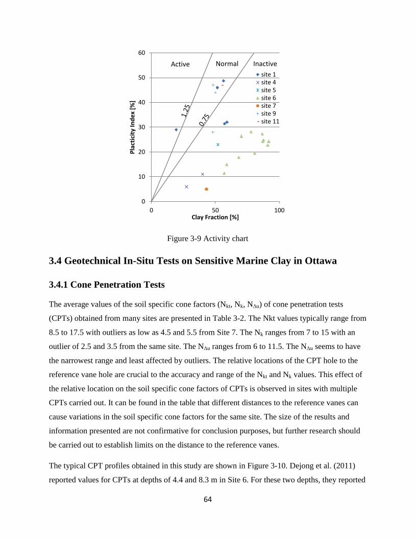
64
Figure 3-9 Activity chart
3.4 Geotechnical In-Situ Tests on Sensitive Marine Clay in Ottawa
3.4.1 Cone Penetration Tests
The average values of the soil specific cone factors (Nkt, Nk, NΔu) of cone penetration tests
(CPTs) obtained from many sites are presented in Table 3-2. The Nkt values typically range from
8.5 to 17.5 with outliers as low as 4.5 and 5.5 from Site 7. The Nk ranges from 7 to 15 with an
outlier of 2.5 and 3.5 from the same site. The NΔu ranges from 6 to 11.5. The NΔu seems to have
the narrowest range and least affected by outliers. The relative locations of the CPT hole to the
reference vane hole are crucial to the accuracy and range of the Nkt and Nk values. This effect of
the relative location on the soil specific cone factors of CPTs is observed in sites with multiple
CPTs carried out. It can be found in the table that different distances to the reference vanes can
cause variations in the soil specific cone factors for the same site. The size of the results and
information presented are not confirmative for conclusion purposes, but further research should
be carried out to establish limits on the distance to the reference vanes.
The typical CPT profiles obtained in this study are shown in Figure 3-10. Dejong et al. (2011)
reported values for CPTs at depths of 4.4 and 8.3 m in Site 6. For these two depths, they reported
0
10
20
30
40
50
60
0 50 100
Pla
ctic
ity
Ind
ex
[%]
Clay Fraction [%]
site 1 site 4 site 5 site 6 site 7 site 9 site 11
Active Normal Inactive
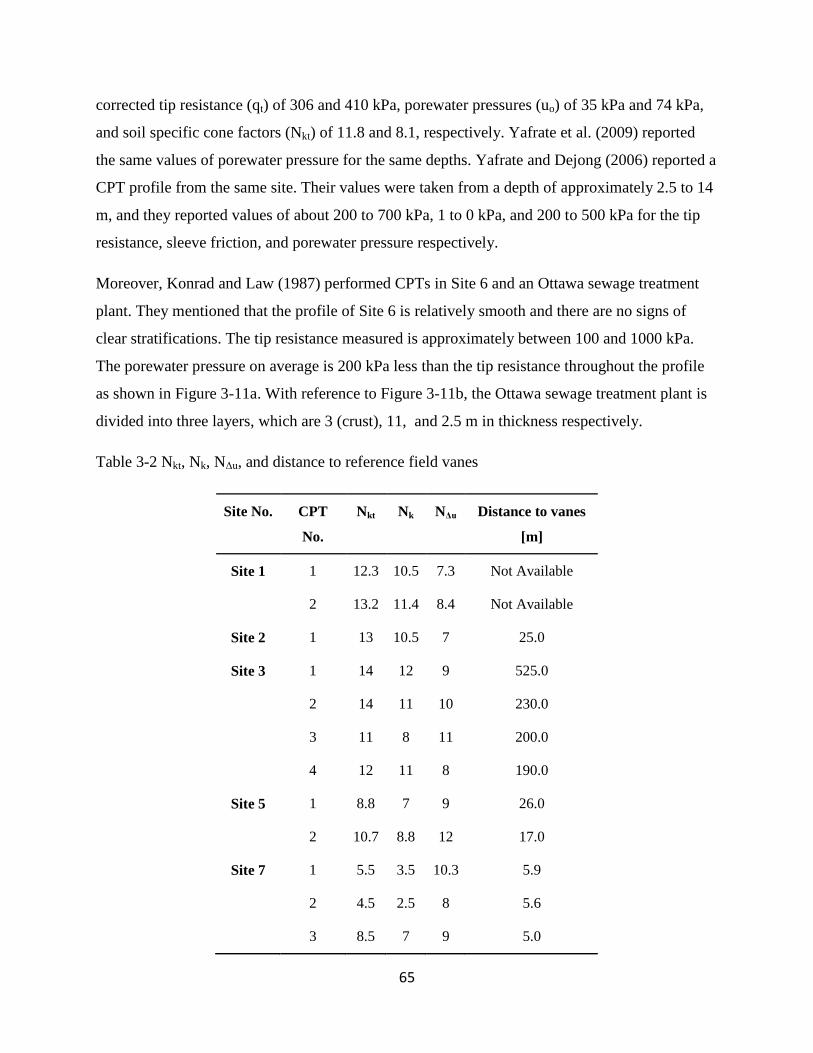
65
corrected tip resistance (qt) of 306 and 410 kPa, porewater pressures (uo) of 35 kPa and 74 kPa,
and soil specific cone factors (Nkt) of 11.8 and 8.1, respectively. Yafrate et al. (2009) reported
the same values of porewater pressure for the same depths. Yafrate and Dejong (2006) reported a
CPT profile from the same site. Their values were taken from a depth of approximately 2.5 to 14
m, and they reported values of about 200 to 700 kPa, 1 to 0 kPa, and 200 to 500 kPa for the tip
resistance, sleeve friction, and porewater pressure respectively.
Moreover, Konrad and Law (1987) performed CPTs in Site 6 and an Ottawa sewage treatment
plant. They mentioned that the profile of Site 6 is relatively smooth and there are no signs of
clear stratifications. The tip resistance measured is approximately between 100 and 1000 kPa.
The porewater pressure on average is 200 kPa less than the tip resistance throughout the profile
as shown in Figure 3-11a. With reference to Figure 3-11b, the Ottawa sewage treatment plant is
divided into three layers, which are 3 (crust), 11, and 2.5 m in thickness respectively.
Table 3-2 Nkt, Nk, NΔu, and distance to reference field vanes
Site No. CPT
No.
Nkt Nk NΔu Distance to vanes
[m]
Site 1 1 12.3 10.5 7.3 Not Available
2 13.2 11.4 8.4 Not Available
Site 2 1 13 10.5 7 25.0
Site 3 1 14 12 9 525.0
2 14 11 10 230.0
3 11 8 11 200.0
4 12 11 8 190.0
Site 5 1 8.8 7 9 26.0
2 10.7 8.8 12 17.0
Site 7 1 5.5 3.5 10.3 5.9
2 4.5 2.5 8 5.6
3 8.5 7 9 5.0

66
Site 8 1 8 6.5 9.5 19.5
2 10 9 9 16.5
3 12 12 8.5 15
Site 9 1 9.5 7 10.1 6
2 14.5 12 11.5 46.8
3 12 10.5 6 52.2
4 10 8.5 8.5 57
5 17.5 15 9.5 46.8
Site 10 1 9 7 8.5 52
2 8.5 8.5 7 118
3 12.5 11 8 84
Site 11 2 10.5 8.5 9.5 54
(a)
0
5
10
15
20
25
30
35
0 2000 4000 6000 8000
Dep
th [
m]
Tip Resistance [kPa]
qc-1
qc-2
0 20 40
Sleeve Friction [kPa]
fs-1
fs-2
0.0 800.0 1600.0
Porewater Pressure [kPa]
u2-1
u2-2

67
(b)
(c)
0
5
10
15
20
25
30
0 4000 8000
Dep
th [
m]
Tip Resistance [kPa]
0 150 300
Sleeve Friction [kPa]
0 600 1200
Porewater Pressure [kPa]
0
2
4
6
8
10
12
14
16
18
0 2500 5000
De
pth
[m
]
Tip Resistance [kPa]
qc-1
qc-2
qc-3
qc-4
0 50 100
Sleeve Friction [kPa]
fs-1 fs-2 fs-3 fs-4
0 400 800
Porewater Pressure [kPa]
u2-1 u2-2 u2-3 u2-4
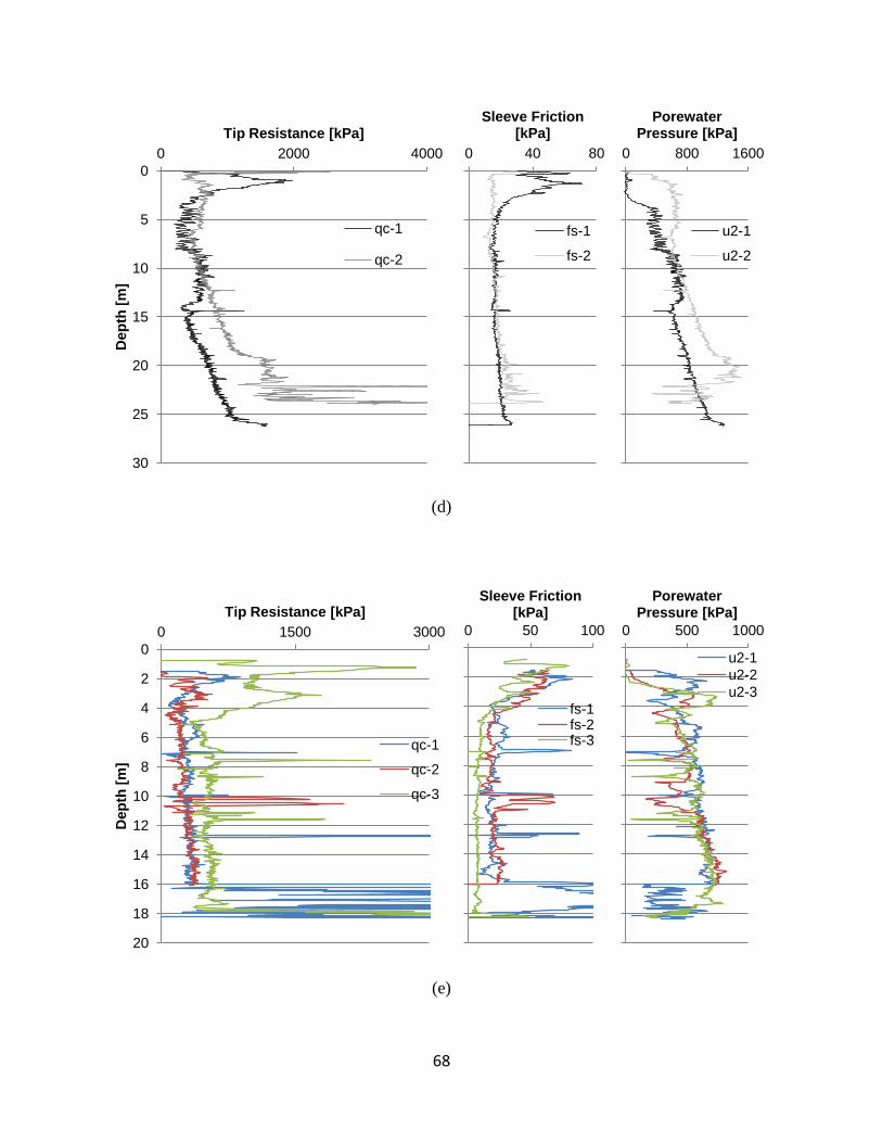
68
(d)
(e)
0
5
10
15
20
25
30
0 2000 4000
Dep
th [
m]
Tip Resistance [kPa]
qc-1
qc-2
0 40 80
Sleeve Friction [kPa]
fs-1
fs-2
0 800 1600
Porewater Pressure [kPa]
u2-1
u2-2
0
2
4
6
8
10
12
14
16
18
20
0 1500 3000
Dep
th [
m]
Tip Resistance [kPa]
qc-1
qc-2
qc-3
0 50 100
Sleeve Friction [kPa]
fs-1 fs-2 fs-3
0 500 1000
Porewater Pressure [kPa]
u2-1
u2-2
u2-3

69
(f)
(g)
0
5
10
15
20
25
30
0 1250 2500
Dep
th [
m]
Tip Resistance [kPa]
qc-1 qc-2 qc-3
0 75 150
Sleeve Friction [kPa]
fs-1 fs-2 fs-3
0 1000 2000
Porewater Pressure [kPa]
u2-1 u2-2 u2-3
0
5
10
15
20
25
30
35
0 2000 4000
Dep
th [
m]
Tip Resistance [kPa]
qc-1
qc-2
qc-3
qc-4
qc-5
0 75 150
Sleeve Friction [kPa]
fs-1 fs-2 fs-3 fs-4 fs-5
0 700 1400
Porewater Pressure [kPa]
u2-1 u2-2 u2-3 u2-4 u2-5

70
(h)
(i)
Figure 3-10 Tip resistance, sleeve friction, and porewater pressure with depth for (a) Site 1 (b)
Site 2 (c) Site 3 (d) Site 5 (e) Site 7 (f) Site 8 (g) Site 9 (h) Site 10 (i) Site 11
0
2
4
6
8
10
12
14
0 2000 4000
Dep
th [
m]
Tip Resistance [kPa]
qc-1
qc-2
qc-3
0
2
4
6
8
10
12
14
0 100 200
Sleeve Friction [kPa]
fs-1 fs-2 fs-3
0
2
4
6
8
10
12
14
0 300 600
Porewater Pressure [kPa]
u2-1 u2-2 u2-3
0
5
10
15
20
25
30
35
0 1250 2500
Dep
th [
m]
Tip Resistance [kPa]
0 35 70
Sleeve Friction [kPa]
0 600 1200
Porewater Pressure [kPa]

71
Figure 3-11 Tip resistance and porewater pressure with depth for (a) Site 6 (b) sewage water
treatment plant in Ottawa. Taken from Konrad and Law (1987)
3.4.2 Standard Penetration Tests
The obtained N60 values from standard penetration tests (SPTs) are shown in Figure 3-12. In
general, the N60 values from SPTs are higher in the top soil and fill layers above the sensitive
marine clay layers and in the till layer below than they are in the clay layer. The SPT N values
for the clay range between 1 and 5, and for the upper crust layer, between 1 and 16. In Sites 4
and 5, there are layers that intercross and those that are not clearly defined. In the other sites,
there may be intercrossing between layers, especially the fill layer and the clay layer beneath it.
In other words, the layer thickness is only an estimation.

72
(a) (b) (c) (d)
(e) (f) (g) (h)
0
10
20
30
40
50
60
70
0 20 40 D
ep
th [
m]
N_Value
0
5
10
15
20
25
0 15 30
Dep
th [
m]
N_Value
0
2
4
6
8
10
12
14
16
18
20
0 20 40
Dep
th [
m]
N_Value
0
2
4
6
8
10
12
14
16
0 5 10
Dep
th [
m]
N_Value
0
5
10
15
20
25
30
35
0 10 20
Dep
th [
m]
N_Value
0
5
10
15
20
25
0 10 20
Dep
th [
m]
N_Value
0
5
10
15
20
0 25 50
Dep
th [
m]
N_Value
0
5
10
15
20
25
0 10 20
Dep
th [
m]
N_Value

73
(i) (j) (k) (l)
(m) (n)
Figure 3-12 N60 from SPTs with depth for (a) Site 1 (b) site 2 (c) Site 3 (d) Site 4 (e) Site 5 (f)
Site 7 (g) Site 8 (h) Site 9 (i) Site 10 (j) Site 11 (k) Site 12 (l) Site 13 (m) Site 14 (n) Site 15
3.4.3 Vane Shear Tests and Undrained Shear Strength
The undrained shear strength values obtained from the vane tests performed on the sites studied
(except for Site 6) are presented in Figure 3-13 along with the shear strength values estimated
from the N60 values. The Canadian Foundation Engineering Manual (2006) presents a correlation
0
1
2
3
4
5
6
7
8
0 7 14 D
ep
th [
m]
N_Value
0
5
10
15
20
25
30
35
0 15 30
Dep
th [
m]
N_Value
0
1
2
3
4
5
6
0 12 24
Dep
th [
m]
N_Value
0
5
10
15
20
25
0 12 24
Dep
th [
m]
N_Value
0
1
2
3
4
5
6
7
8
0 50
Dep
th [
m]
N_Value
0
1
2
3
4
5
6
7
8
0 15 30
Dep
th [
m]
N_Value

74
between the undrained shear strength of clay soils and N60 from SPTs in Table 3.3 in the manual.
However, from Figure 3-13, it can be found that there is an underestimation of the undrained
shear strength which was estimated from the SPTs compared to the vane results with all of the
sites taken into consideration. Therefore, the results suggest a disagreement of the results
between the field SPTs and vanes for the marine clays in Ottawa on the one hand, and the
correlation presented in Table 3.3 in the aforementioned manual on the other hand.
Konrad and Law (1987) mentioned that vanes measure the undrained shear strength in the
horizontal direction as the vanes turn horizontally in soil. In addition, the horizontal effective
stress is lower than the vertical effective stress for normally consolidated and lightly
overconsolidated soils such as sensitive marine clays in Ottawa. Therefore, the undrained shear
strength measured by using vanes is lower than that measured from CPTs and triaxial tests on
vertically sampled specimens.
Yafrate and Dejong (2006) reported values of undrained shear strength of 20 and 34 kPa at 4.5
and 8.5 m, respectively, from field vanes at Site 6. Dejong et al. (2011) and Yafrate et al. (2009)
reported undrained shear strength values of 20 and 34 kPa from field vanes at depths of 4.4 and
8.3 m, respectively, for the same site.
The results of the undrained shear strength values obtained from the vane tests presented in
Figure 3-13 are in agreement with those reported in previous studies. For example, Eden and
Crawford (1957) performed tests for five vane profiles in Ottawa. The first profile showed a
slight increase in the shear strength with depth at approximately 21 kPa near the surface and 72
kPa around a depth of 18 m. The second profile showed a decrease and then an increase in the
shear strength halfway with depth at approximately 70 kPa near the surface, 32 kPa at a depth of
14.6 m, and 110 kPa at a depth of 27 m. The third profile had a general trend of decrease and a
shear strength range between 57 and 145 kPa. The fourth profile showed a constant trend in the
shear strength with depth between 57 and 91 kPa to a depth of 12 m. The fifth profile showed a
slight increase in the shear strength with depth between 57 and 145 kPa to a depth of 15 m. The
fissured or crust part of the clay seemed to have approximately the maximum or higher value of
shear strength of the soil profile. The crust layer had shear strength of 62 kPa in the first profile
and 187 kPa in the second profile. They mentioned that the field vane tests (FVTs) can give
results that are many times higher than the laboratory results. Mitchell (1970) reported vane test

75
results for Site 6 from block samples as 127.5, 156.9, and 166.7 kPa for depths of 13.7, 16.1 and
19.0 m respectively. Dayal (1970) reported undrained shear strength values from other
researchers, such as Crawford (1961), Crawford (1968), and Crawford and Eden (1965), for
sensitive marine clays in a range of 9.5 to 383 kPa.

76
(a) (b)
(c) (d)
0
10
20
30
40
50
60
70
0 100 200 300
Dep
th [
m]
Undrained Shear Strength [kPa]
FVT
SPT
0
5
10
15
20
25
30
35
0 50 100 150
Dep
th [
m]
Undrained Shear Strength [kPa]
Lab
SPT
0
5
10
15
20
0 25 50
De
pth
[m
]
Undrained Shear Strength [kPa]
Lab
SPT
FVT
0
5
10
15
20
0 20 40 60
De
pth
[m
]
Undrained Shear Strength [kPa]
Lab
SPT

77
(e) (f)
(g) (h)
0
5
10
15
20
25
30
35
0 50 100 150 D
ep
th [
m]
Undrained Shear Strength [kPa]
Lab
FVT
SPT
0
5
10
15
20
25
0 50 100 150
Dep
th [
m]
Undrained Shear Strength [kPa]
FVT
SPT
0
2
4
6
8
10
12
14
16
18
0 75 150
Dep
th [
m]
Undrained Shear Strength [kPa]
FVT
SPT
0
5
10
15
20
25
0 50 100
Dep
th [
m]
Undrained Shear Strength [kPa]
FVT
SPT

78
(i) (j)
(k) (l)
0
2
4
6
8
10
0 150 300 D
ep
th [
m]
Undrained Shear Strength [kPa]
FVT
SPT
0
5
10
15
20
25
30
35
40
0 150 300
Dep
th [
m]
Undrained Shear Strength [kPa]
FVT
SPT
0
2
4
6
0 100 200 300
Dep
th [
m]
Undrained Shear Strength [kPa]
FVT
SPT
0
5
10
15
20
25
0 50 100 150
Dep
th [
m]
Undrained Shear Strength [kPa]
FVT
SPT

79
(m) (n)
Figure 3-13 Undrained shear strength from field vane tests (FVT), lab vane tests (LVT), and/or
SPT correlation for (a) Site 1 (b) Site 2 (c) Site 3 (d) Site 4 (e) Site 5 (f) Site 7 (g) Site 8 (h) Site
9 (i) Site 10 (j) Site 11 (k) Site 12 (l) Site 13 (m) Site 14 (n) Site 15
3.4.4 FVTs and LVTs
The objective of this section is to compare the results obtained from FVTs performed at Site 6
and laboratory vane tests (LVTs) performed on undisturbed samples obtained from the same site.
For the former, a rotation rate of 0.1 degree/s was used in accordance with ASTM D2573. The
vane was the lower end tapered type with dimensions of 130 x 65 mm. For the latter, a rotation
rate of 1 degree/s was used in accordance with ASTM D4648. The vane had a cross section that
was 19 x 12.7 mm. Ten rapid rotations were performed before determining the remolded shear
strength for both types of tests. Landon-Maynard et al. (2011) mentioned that there should be an
adjustment between the field and the lab vanes as a result of the rotation rate. They indicated that
the shear strength should be increased by 13% for each order of magnitude of increase in the rate
of rotation. Therefore, the LVT results should be multiplied by a factor of 2.3 (0.13*10+1) to
0
1
2
3
4
5
6
7
8
0 150 300 D
ep
th [
m]
Undrained Shear Strength [kPa]
FVT
SPT
0
1
2
3
4
5
6
7
8
0 75 150
Dep
th [
m]
Undrained Shear Strength [kPa]
FVT
SPT

80
correct for the rotation rate as the lab vanes were turned at 10 times the rate of the field vanes. It
can be seen from Figures 3-14a and b that in the undrained and remolded shear strengths from
both tests, the use of the lab vanes results in significant underestimation (or overestimation in
some cases) compared to the use of field vanes. The difference could be several orders of
magnitude. Therefore, this type of correction may not be applicable for sensitive marine clays in
Ottawa due to the high dependency on the rate of rotation. However, the sensitivity seems to
have a somewhat better agreement between the field and lab vanes than the undrained and
remolded shear strength. The adjusting of the lab vanes to the same rate of rotation as the field
vanes is an option to consider for future research. The ASTM also recommends the correction
indicated by Ladd (1975) and Larsson (1980) by multiplying the result by a factor obtained
based on the plasticity index of the soil. This correction has been applied to the results. The
ASTM standard recognizes that soft soils may be tested in the field with the maximum rate in the
average specified (0.05-0.2 degree/s). Due to the sensitivity of marine clays in Ottawa, strength
may be regained during the testing, thus resulting in difficulties, especially in determining the
remolded shear strength. At low rates of rotation, the maximum shear strength or well defined
failure point may not appear even after turning the vanes to more than 90 degrees. Figures 3-15a
and b show that that increases in shear strength may continue as a result of a slow rotational rate
which allows sensitive marine clays in Ottawa to regain strength during testing. The gain in
strength may be due to the gain of strength at the vanes or on the turn rods in the form of rod
friction. Figure 3-15a shows a gain of strength that is dominated by the soil on the vane as it is at
a shallower depth than that of Figure 3-15b. Figure 3-15b on the other hand, shows the regain of
strength dominated by the soil which acts on the turn rods in the form of rod friction as it is
deeper than that in Figure 3-15a and contains up and down waves as a result of failure envelopes.

81
Figure 3-14 Results of Nilcon field and miniature lab vanes in Site 6 (a) undrained shear strength
with depth (b) remolded shear strength with depth (c) sensitivity with depth
Figure 3-15 Remolded shear strength with rotation angle from Nilcon field vanes for rotational
rate of 0.1 degree/s in Site 6 at a depth of (a) 3.68 m, and (b) 16.68 m
0
5
10
15
20
25
0 30 60 90
Dep
th [
m]
Undrained Shear Strength [kPa]
0
5
10
15
20
25
0 10 20 30
Dep
th [
m]
Remolded Shear Strength [kPa]
0
5
10
15
20
25
0.0 20.0 40.0
Dep
th [
m]
Sensitivity
Nilcon Field Vanes
Miature Lab Vanes

82
3.4.5 Shear Wave Velocity Measurements
The Canadian Foundation Engineering Manual (2006) presents a correlation between the site
class on the one hand and the soil shear wave velocity or the undrained shear strength on the
other hand in Table 6.1A in the manual. There are seven site classes from A to F that are used to
find site coefficients for seismic design purposes. The range of the values of the shear wave
velocities (over 180 m/s and under 1500 m/s) and undrained shear strength (over 50 kPa and
under 100 kPa) are used as the limits to define site classes.
For sites with available shear wave velocity measurements and vanes, comparisons between the
site class defined by using the shear wave velocity measurements and undrained shear strength
are presented in Figure 3-16. For ease of explanation, Method 1 represents the site class that uses
the shear wave velocity measurement, and Method 2 represents the site class that uses undrained
shear strength. For Site 7, Method 1 renders that the site class ranges between D and E while
Method 2 renders the site class that fluctuates between C, D and E. At a depth of approximately
3 to 4 m, Method 1 peaks in Class D while Method 2 peaks in Class C. It is observed that the
general trend of the two methods is in agreement, but in different site classes, which indicates a
site class limits problem. In Site 8, there is a misestimation of a whole class letter. In other
words, Method 1 results in Classes D and E while Method 2 results in Classes C and D. Site 9
has five shear wave velocity profiles and one vane profile. Method 2 ranges between Classes D
and E, and approaches Class C near a depth of approximately 3 m. Method 2 results in five
different trends of site classifications from five profiles. All of the profiles from Method 1 range
between Classes D and E, except for Figure 18(c) which extends to Class C near the surface. In
Fig. 18(g), the site class extends into Class D near the bottom of the profile while Method 2
profiles fluctuate between Classes D and E throughout and near Class C near the surface. As
there may be underestimations in the estimation of undrained shear strength in the Canadian
Foundation Engineering Manual for sensitive marine clays in Ottawa, there is disagreement in
the estimation of site class from the undrained shear strength profiles. The number of data sets is
not conclusive but raises the issue for future research. A point to mention is that according to the
seismic site class map of Ottawa in the National Building Code of Canada (NBCC), all five
classes from A through F are found in Ottawa.

83
(a) (b)
(c) (d)
0
2
4
6
8
10
12
14
16
18
50 100 150 200 250 D
ep
th [
m]
Shear Wave Velocity [m/s]
Class E Class D
0
2
4
6
8
10
12
14
16
18
0 50 100 150
Dep
th [
m]
Shear Strength [kPa]
Class E Class D Class C
0
5
10
15
20
0 100 200 300
Dep
th [
m]
Shear Strength [kPa]
Class E Class D
0
5
10
15
20
20 40 60 80 100 120
Dep
th [
m]
Shear Strength [kPa]
Class E Class D Class C

84
(e) (f)
(g) (h)
0
4
8
12
16
20
24
0 200 400 600
Dep
th [
m]
Shear Wave Velocity [m/s]
Class E Class D Class C
0
4
8
12
16
20
24
0 50 100 150
Dep
th [
m]
Shear Strength [kPa]
Class E Class D Class C
0
4
8
12
16
20
24
0 200 400 600
Dep
th [
m]
Shear Wave Velocity [m/s]
Class E Class D Class C
0
4
8
12
16
20
24
0 50 100 150
Dep
th [
m]
Shear Strength [kPa]
Class E Class D Class C

85
(i) (j)
(k) (l)
0
4
8
12
16
20
24
0 200 400 600
Dep
th [
m]
Shear Wave Velocity [m/s]
Class E Class D Class C
0
4
8
12
16
20
24
0 50 100 150
Dep
th [
m]
Shear Strength [kPa]
Class E Class D Class C
0
4
8
12
16
20
24
0 200 400 600
Dep
th [
m]
Shear Wave Velocity [m/s]
Class E Class D Class C
0
4
8
12
16
20
24
0 50 100 150
Dep
th [
m]
Shear Strength [kPa]
Class E Class D Class C

86
(m) (n)
Figure 3-16 Shear wave velocity and shear strength with depth and site classification according
to the Canadian Engineering Foundation Manual for (a) Site 7 (b) Site 7 (c) Site 8 (d) Site 8 (e)
Site 9 (f) Site 9 (g) Site 9 (h) Site 9 (i) Site 9 (j) Site 9 (k) Site 9 (l) Site 9 (m) Site 9 (n) Site 9
3.5 Interface Shear Strength and Behavior
An understanding of the interface shear behavior between sensitive marine clays and structures is
significantly important for the safe and cost effective designs of several geotechnical structures
(e.g., friction piles, retaining walls, and anchors). Taha (2010) and Taha and Fall (2010)
performed a series of interface shear testing on marine clay samples from Ottawa to examine the
shear behaviour and strength at the interfaces of marine clay - steel and marine clay - concrete. A
series of consolidated drained and unconsolidated undrained shear tests were performed to
examine the interface with steel. The samples had different overconsolidation ratios (OCRs) and
saturation values. They noticed that by applying a normal stress of 250 kPa, the clay alone
exhibits higher shear resistance than in the interface of the marine clay - steel. However, at
normal stresses higher than 250 kPa, shear resistance of the clay alone is the same as that of the
interface zone. They attributed this behavior to the tendency of marine clays to remold at higher
0
4
8
12
16
20
24
0 200 400 600
Dep
th [
m]
Shear Wave Velocity [m/s]
Class E Class D Class C
0
4
8
12
16
20
24
0 50 100 150
Dep
th [
m]
Shear Strength [kPa]
Class E Class D Class C

87
normal stresses. They also found that an increase in the steel surface roughness can increase the
resistance shear strength as a result of the increase of the interlocking forces between the clay
and steel. This is similar to the findings of Tsubakihara and Kisheda (1993). Moreover, they
found that denser Ottawa marine clay has higher interlocking forces between the clay and steel.
They showed that increasing the surface roughness increases the vertical deformation or
displacement of the marine clay, and small changes in the surface roughness (1to 5 µm) does not
induce significant deformation differences. When the surface roughness increases, the internal
friction angle increases. Therefore, when the internal friction angle approaches the internal
friction coefficient of the soil, shear failure would occur in the soil rather than in the interface
(Hamid and Miller 2009; Taha, 2010; Taha and Fall, 2010). The effect of the OCR decreases
with increasing the normal stress on the soil. However, the shear strength of marine clay
increases with increasing the OCR as a result of higher density associated with a higher OCR.
Also, the angle of internal friction is higher when there is increase in the OCR (DeJong and
Westgate 2005; Taha, 2010; Taha and Fall,. 2010). As the degree of saturation decreases or the
suction increases, the interface shear strength increases (Fleming et al. 2006; Hamid and Miller
2009; Taha, 2010; Taha and Fall 2010). Similar to the OCR effect, as the density increases, the
interface dry density increases. This is attributed to the increased density and higher interlocking
forces between the clay and steel. Therefore, Taha (2010) suggested that the soil be compacted in
order to obtain higher interface shear strength.
For the concrete-clay interface, it was observed that the shear resistance is in the sensitive clay
layer above the interface layer up to a deformation of 2%. After a displacement of 2%, the shear
strength increased as the roughness increased. It was found that the difference in the shear
strength between a roughness of 6.5 and 10 µm is not as significant as that between 10 and 20
µm. The reason is attributed to the interlocking forces between the soil and concrete and the
accuracy of the surface roughness measurements. Also, there is higher shear strength because
there is higher normal stress. It is worth noting that the surface roughness is not significant when
there is low normal stress (250 kPa) as the interlocking forces between the soil and concrete
require high stress to break. The angle of the interface friction increased as the surface roughness
increased, but was not sensitive to small changes, such as 6.5 to 10 µm (Taha and Fall 2010).
Clay at the interface deformed less than pure clay, especially at high shear increments. The
reason is that concrete roughness can cause remolding and reorientation of the clay particles. The
88
shear stress and displacement were found to be independent of the consolidation state of the clay
(Taha et al. 2010; Tsubakihara and Kisheda 1993).
The interface shear strength increased as the salt or sodium chloride concentration increased
(Taha et al. 2010). Torrance (1975) attributed this behavior to the positive charges of the clay
particles which exhibit negative charges on their surfaces. Higher ion concentrations reduce the
effect of the charges on the edges which make the clay particles less repulsive to each other. It
also facilitates the formation bonds between the positively charged edges and negatively charged
surface of the clay particles. The interface shear strength increases as the degree of saturation
decreases and the suction increases. This can be explained by the increase in the interlocking
forces between the clay and concrete and between the clay particles as the suction increases. It
was found that the peak interface shear strength can be achieved within a range of 1% to 3% of
displacement (Taha and Fall, 2010). The interface shear strength increased as the density
increased. This is because there are higher interlocking forces between the clay and concrete in
denser soils and there is a larger interaction area between the clay and concrete (DeJong and
Westgate 2005; DeJonge and Westgate 2009).
3.6 Consolidation Behavior
3.6.1 Preconsolidation Pressure and Over Consolidation Ratio
The preconsolidation pressure is one of the most important characteristics of clays: it is the
vertical effective stress beyond which large strains take place, particularly in sensitive clays
(Leroueil et al. 1983). The preconsolidation pressures and OCRs of the sensitive marine clays in
the studied sites are shown in Figure 3-17. It is evident that the preconsolidation pressures
generally increase with depth, while the OCRs slightly decrease with depth. The
preconsolidation pressure ranges between 40 and 660 kPa for all of the sites. The OCR ranges
between 1.4 and 7.1 for all of the sites.
Sensitive marine clay in Ottawa is known to have a so called "card-house" structure. This type of
structure does not experience significant settlement before reaching the preconsolidation
pressure. After reaching the preconsolidation stress, the soil experiences a sudden high
settlement and clay plates orient into a form parallel to each other and perpendicular to the
direction of the consolidation (Taha, 2010). Therefore, the void ratio is reduced, and bonds

89
between the soil particles break. As a result, remolded or disturbed samples may have flatter
consolidation curves than intact samples and this may lead to underestimating of the
preconsolidation pressure (Quigley and Thompson 1966; Taha, 2010).
The results presented in Figure 3-17 are in agreement with those reported by other researchers.
For instance, preconsolidation pressure and OCR were determined to be 150 kPa and 1.1
respectively for samples obtained by Taha (2010). Leroueil (1999) reported that the OCR for
eastern Canada clays ranges between 1.2 and 5. Dejong et al. (2011) reported an OCR between
1.8 and 1.5 for depths of 4.4 and 8.3 m respectively in Site 6. Rasmussen (2012) reported
preconsolidation pressure, overburden stress, and OCR ranges of 100 to 200 kN/m2, 39 to 172
kN/m2, and 1.0 to 3.2 respectively for the Ottawa area. Eden and Crawford (1957) reported a
preconsolidation pressure for sensitive marine clays in Ottawa of 71.8 kPa. Mitchell (1970)
reported a preconsolidation value of 441.3 kPa at Site 6 for block samples obtained at depths of
13.7, 16.1, and 19.0 m. He also reported overburden stress values of 127.5, 147, and 176.5 kPa
for the same depths.
The preconsolidation pressure profile for Site 6 was supplied by the National Research Council
of Canada and published by Hinchberger and Rowe (1998). This profile has a pattern of
increases with depth from approximately 48 to 171 kPa at a depth of 1 to 17 m, respectively.

90
Figure 3-17 (a) Preconsolidation pressure with depth (b) OCR with depth for all of the sites
3.6.2 Compression Index
The compression indexes of the marine clays of the studied sites are shown in Figure 3-18. The
compression indexes were determined from the slope of the virgin compression line from the
oedometer tests. There does not seem to be a clear relationship with depth. The Cc ranges
between 0.44 and 2.01 for Site 6 and between 0.4 and 2.24 for all of the other sites.
The compression index (Cc ) was determined to be 2.44 for the samples tested by Taha (2010).
They mentioned that the calculated Cc is 2.34 verifies the formula proposed by Leroueil (1999):
20.65 0.15 0.5c o oC e e
Holtz and Kovacs (1981) indicated that the Cc of Canadian marine clays including those in the
Ottawa region is between 1 and 4. The Cc profile for Site 6 was supplied by the National
Research Council of Canada, and published by Hinchberger and Rowe (1998).The Cc values
range between approximately 0.25 and 1.9. The values generally show a pattern of increase, from
a depth of approximately 1 to 10 m, then a pattern of decrease, from a depth of 10 to 19 m. An
average value of 0.65 was designated by Hinchberger and Rowe (1998).
0
5
10
15
20
25
30
35
40
45
50
0 200 400 600 800 D
ep
th [
m]
Preconsolidation Pressure [kPa]
site 1 site 2 site 3 site 4 site 5 site 8 site 9 site 10 site 11 site 12 site 13
0
5
10
15
20
25
30
35
40
45
50
0 2 4 6 8
Dep
th [
m]
OCR
site 1
site 2
site 4
site 5
site 9
site 12

91
Sensitive marine clays in Ottawa do not have a constant compression index, but the compression
index decreases as the stress increases past the yield pressure (Mitchell 1970; Rasmussen 2012).
Sensitive marine clays in Ottawa exhibit high initial values in the compression index as a result
of the sudden break of the cementation bonds between the clay particles of the clay (Jarrett 1967;
Rasmussen 2012; Walker and Raymond 1968).
Figure 3-18 Compression index with depth
3.6.2.1 Example of Consolidation Curve
Figure 3-19 is a typical example of an oedometer test for sensitive marine clay in Ottawa. It can
be seen that the slope of the curve beyond the preconsolidation pressure decreases with
increasing the stress. Therefore, there could be more than one compression index for the same
soil. From general engineering practices, it is recommended that the compression index and other
indices and coefficients from the loading cycle that is closest to the field condition be
determined. Sometimes engineers use the stage with the highest compression index for a higher
factor of safety in designs, which is usually the stage directly after the preconsolidation pressure.
0
5
10
15
20
25
30
35
40
45
50
0 1 2 3 D
ep
th [
m]
Compression Index
site 1
site 2
site 3
site 4
site 5
site 6
site 8
site 9
site 10
site 11
site 12
site 13

92
Figure 3-19 also shows a sudden break of the soil at the preconsolidation pressure. The reason
behind this behaviour is the cardhouse structure of the soil. The porewater and the soil skeleton
take the stress and resist consolidation. Eventually, they fail, and cause a high degree of
settlement at the break point (Taha,. 2010). Therefore, for determining the preconsolidation
pressure, it is necessary to avoid the loading of the soil with double the stress near the break
point (ASTM D 2435). The ASTM D 2435 standard recommends the use of a double scheme for
loading. However, this can cause a reduction in accuracy when determining the preconsolidation
pressure.
Figure 3-19 Consolidation curve for a depth of 3.8 m at Site 6
3.6.2 Recompression Index
Figures 3-20 show recompression indexes with depth for the studied sites. It can be observed that
there is no clear relationship between the recompression indexes and depth. The recompression
index for Site 6 ranges between 0.03 and 0.09 and between 0.02 and 0.09 for all of the other
sites. It can be seen from Table 3-3 that the ratio of the compression index to the recompression
index ranges between 3.4 and 76.5 with an average of 36.1 with two outliers of 140.7 at Site 2
and 106 at Site 11.
0.7
0.9
1.1
1.3
1.5
1.7
1.9
2.1
2.3
2.5
1 100 10000
Void
Ratio,
e
Stress (kPa)

93
Sensitive marine clays in Ottawa in general have low recompression indexes (Crawford 1968).
Rasmussen (2012) reported recompression indexes between 0.011 and 0.072 for stresses of 5 to
50 kPa. She also reported swell indexes that range between 0.028 and 0.12 for stresses between
the end of her oedometer tests and 50 kPa. She attributed the low values of the swell indexes to
the high stress that she had subjected her samples. On average, she had subjected her samples to
1500 kPa while the overburden stresses of the samples were between 39 and 172 kPa. Therefore,
there is a high degree of destruction to the internal structure of the clay. A value of 0.025 for Cr
was estimated by Hinchberger and Rowe (1998) based on a study by Leroueil et al. (1983) on
Site 6.
Figure 3-20 Recompression index with depth from oedometer tests
0
10
20
30
40
50
60
0 0.05 0.1 0.15
Dep
th [
m]
Recompression Index
site 1
site 2
site 3
site 4
site 5
site 6
site 8
site 9
site 10
site 11
site 12
site 13

94
Table 3-3 Compression index to recompression index ratios
Site Depth [m] Cc/Cr Site Depth [m] Cc/Cr
1 6.1 37.5 6 2.6 10.8
1 30.8 42.5 6 4.1 28.7
1 12.5 45.0 6 6.4 8.8
1 49.1 20.3 6 8.7 14.4
2 9.1 18.5 6 12.6 8.7
2 3.4 140.7 6 14.0 8.8
2 8.0 15.3 6 15.5 10.9
2 5.0 38.5 6 17.1 10.2
2 9.5 20.0 6 18.6 9.4
2 3.6 63.0 9 7.6 37.0
2 12.4 39.5 9 15.2 62.0
3 12.2 33.5 10 7.6 74.7
4 12.2 16.7 10 10.7 37.0
4 13.7 30.3 11 7.8 51.0
4 6.4 14.3 11 16.5 106.0
5 13.7 34.0 12 3.8 29.8
5 12.2 16.7 12 5.6 34.5
5 9.5 76.5 13 11.0 31.0
8 4.6 50.5 13 4.6 34.7
8 13.7 36.5 13 4.8 46.0
3.6.3 Coefficient of Consolidation
Figure 3-21 shows the variation of the coefficient of consolidation with pressure in the same
graph with the consolidation curves. The testing results are from Sites 2 and 3. There is no clear
pattern between the pressure and the coefficient of consolidation. Also, there is no clear pattern
of increase or decrease in the coefficient of consolidation with pressure in the recompression or
virgin compression portion of the consolidation curve.

95
Figure 3-22 shows the variation of the coefficient of consolidation with stress from the
oedometer testing for the sites under study. The coefficient of consolidation was not determined
for all of the stress intervals due to the lack of the availability of the data. The coefficient of
consolidation of all the sites was determined by using Taylor's square root of time fitting method
(Holtz and Kovacs 1981). Due to the variability of the coefficient of consolidation, it is
recommended that the value of the stress closest to the field condition is used. For the other sites
in the study, the t90 ranged between 4 and 139 minutes which is a relatively large range. On the
other hand, the coefficient of consolidation ranged between 8.99x10⁻⁵
and 3.3x10⁻³
cm2/s.
The coefficient of consolidation generally decreases with increases in the stress. However, it can
increase then decrease with increasing stress. As the stress increases, the soil structure and the
porewater take the load and resist compression. At this point, there is low consolidation in the
soil. Eventually, this structure breaks and causes the rearrangement of the soil structure and
increases the coefficient of consolidation. Table 3-4 is a summary of t90 and the coefficient of
consolidation relative to the stress interval, depth, and preconsolidation pressure from oedometer
tests for the sites studied.
Lo et al. (1976) performed consolidation tests by using large (11.28 cm x 5.08 cm) samples and
small (5.08 cm x 1.27 cm) samples, and they found that the smaller samples yielded values of Cv
that are an order of one or two magnitudes less than the larger samples (Taylor 1948). They
attributed this behavior to higher disturbance associated with the trimming and preparation of
smaller samples (Bozozuk 1971; Zelst 1948), higher hydraulic gradients because of a shorter
drainage distance, and larger strain rates in the early stages of consolidation. They also attributed
this behavior to temperature and mechanical effects from sampling. Lo et al. (1976) reported
values of Cv for different depths and load increments. For small samples, the values of Cv are
0.027 and 0.045 cm2/s for depths of 2.4, 2.5, and 3.4 m, and pressure increments of 38.3 to 88.4
kPa, respectively. For 15.24 cm x 5.08 cm samples of the same increment at a depth of 2.4 m, the
Cv was 2.75 cm2/s from the consolidation testing and 4.74 cm
2/s from pore pressure dissipation
testing. In large samples at depths of 4.3 and 11.1 m and pressure increments of 43.1 to 82.4 kPa
and 72.8 to 99.6 kPa respectively, the Cv values are 2.67 and 2.59 cm2/s. Dayal (1970) reported
coefficients of consolidation from other researchers, such as Crawford (1961), Crawford (1968),
and Crawford and Eden (1965), for sensitive marine clays, which are 1*10-2
to 1*10-5
cm2/s.

96
(a) (b)
(c) (d)

97
(e) (f)
(g) (h)

98
(i) (j)
(k) (l)
Figure 3-21 Consolidation curve and the coefficient of consolidation with pressure from oedometer tests
for Site 2 at depths of (a) 3.43 m (b) 8.0 m (c) 4.95 m (d) 9.45 (e) 3.58 m (f) 12.42 m and for Site 3 at
depths of (g) 3.43 m (h) 8.0 m (i) 4.95 m (j) 9.45 (k) 3.58 m (l) 12.42 m

99
(a) (b)
(c) (d)
(e) (f)
(g) (h)
5.0E-05
3.0E-04
5.5E-04
8.0E-04
1.1E-03
1.3E-03
1.6E-03
1.8E-03
0 200 400 600 800 1000
Co
eff
icie
nt
of
co
ns
oli
da
tio
n a
t d
ep
th o
f 2.6
m
[cm
^2/s
]
Stress [kPa]
5.0E-05
3.0E-04
5.5E-04
8.0E-04
1.1E-03
1.3E-03
1.6E-03
1.8E-03
0 200 400 600 800 1000
Co
eff
icie
nt
of
co
nso
lid
ati
on
at
de
pth
of
4.1
m
[cm
^2/s
]
Stress [kPa]
5.0E-05
3.0E-04
5.5E-04
8.0E-04
1.1E-03
1.3E-03
1.6E-03
1.8E-03
0 200 400 600 800 1000
Co
eff
icie
nt
of
co
ns
oli
da
tio
n a
t d
ep
th o
f 6.4
m
[cm
^2/s
]
Stress [kPa]
5.0E-05
3.0E-04
5.5E-04
8.0E-04
1.1E-03
1.3E-03
1.6E-03
1.8E-03
0 200 400 600 800 1000
Co
eff
icie
nt
of
co
nso
lid
ati
on
at
de
pth
of
8.7
m
[cm
^2/s
] Stress [kPa]
5.0E-05
3.0E-04
5.5E-04
8.0E-04
1.1E-03
1.3E-03
1.6E-03
1.8E-03
0 200 400 600 800 1000
Co
eff
icie
nt
of
co
ns
oli
da
tio
n a
t d
ep
th o
f 12.6
m
[cm
^2/s
]
Stress [kPa]
5.0E-05
3.0E-04
5.5E-04
8.0E-04
1.1E-03
1.3E-03
1.6E-03
1.8E-03
0 200 400 600 800 1000
Co
eff
icie
nt
of
co
nso
lid
ati
on
at
de
pth
of
14.0
m
[cm
^2/s
]
Stress [kPa]
5.0E-05
3.0E-04
5.5E-04
8.0E-04
1.1E-03
1.3E-03
1.6E-03
1.8E-03
0 200 400 600 800 1000
Co
eff
icie
nt
of
co
ns
oli
da
tio
n a
t d
ep
th o
f 15.5
m
[cm
^2/s
]
Stress [kPa]
5.0E-05
5.5E-04
1.1E-03
1.6E-03
2.1E-03
2.6E-03
3.1E-03
0 200 400 600 800 1000
Co
eff
icie
nt
of
co
nso
lid
ati
on
at
de
pth
of
17.1
m
[cm
^2/s
]
Stress [kPa]

100
(i) (j)
(k) (l)
(m) (n)
(o) (p)
5.0E-05
5.5E-04
1.1E-03
1.6E-03
2.1E-03
2.6E-03
3.1E-03
0 200 400 600 800 1000
Co
eff
icie
nt
of
co
ns
oli
da
tio
n a
t d
ep
th o
f 18.6
m
[cm
^2/s
]
Stress [kPa]
0.0E+00
1.0E-03
2.0E-03
3.0E-03
4.0E-03
5.0E-03
6.0E-03
0 200 400 600 800 1000
Co
eff
icie
nt
of
co
ns
oli
da
tio
n a
t d
ep
th o
f 9.1
m s
ite 2
[c
m^
2/s
]
Stress [kPa]
0.0E+00
1.0E-03
2.0E-03
3.0E-03
4.0E-03
5.0E-03
6.0E-03
7.0E-03
0 200 400 600 800 1000
Co
eff
icie
nt
of
co
ns
oli
da
tio
n a
t d
ep
th o
f 12.2
m s
ite 3
[c
m^
2/s
]
Stress [kPa]
0.0E+00
2.0E-03
4.0E-03
6.0E-03
8.0E-03
0 200 400 600 800 1000
Co
eff
icie
nt
of
co
ns
oli
da
tio
n a
t d
ep
th o
f 12.2
m s
ite 4
[c
m^
2/s
] Stress [kPa]
0.0E+00
5.0E-03
1.0E-02
1.5E-02
2.0E-02
2.5E-02
0 200 400 600 800 1000
Co
eff
icie
nt
of
co
ns
oli
da
tio
n a
t d
ep
th o
f 13.7
m s
ite 4
[c
m^
2/s
]
Stress [kPa]
0.0E+00
5.0E-04
1.0E-03
1.5E-03
2.0E-03
2.5E-03
3.0E-03
0 200 400 600 800 1000
Co
eff
icie
nt
of
co
ns
oli
da
tio
n a
t d
ep
th o
f 13.7
m s
ite 8
[c
m^
2/s
]
Stress [kPa]
0.0E+00
2.0E-04
4.0E-04
6.0E-04
8.0E-04
1.0E-03
1.2E-03
0 200 400 600 800 1000
Co
eff
icie
nt
of
co
ns
oli
da
tio
n a
t d
ep
th o
f 7.6
m s
ite 9
[c
m^
2/s
]
Stress [kPa]
0.0E+00
1.0E-03
2.0E-03
3.0E-03
4.0E-03
0 200 400 600 800 1000
Co
eff
icie
nt
of
co
ns
oli
da
tio
n a
t d
ep
th o
f 7.6
m s
ite 1
0
[cm
^2/s
]
Stress [kPa]

101
(q) (r)
(s) (t)
(u) (v)
Figure 3-22 Coefficient of consolidation with stress from oedometer tests for a depth of (a) 2.6 m
Site 6 (b) 4.1 m Site 6 (c) 6.4 m Site 6 (d) 8.7 m Site 6 (e) 12.6 m Site 6 (f) 14.0 m Site 6 (g) 15.5
m Site 6 (h) 17.1 m Site 6 (i) 18.6 m Site 6 (j) 9.1 m Site 2 (k) 12.2 m Site 3 (l) 12.2 m Site 4 (m)
13.7 m Site 4 (n) 13.7 m Site 8 (o) 7.6 m Site 9 (p) 7.6 m Site 10 (q) 10.7 m Site 10 (r) 7.8 m Site
11 (s) 16.5 m Site 11 (t) 11.0 m Site 13 (u) 4.6 m Site 13 (v) 4.8 m Site 13
0.0E+00
1.0E-03
2.0E-03
3.0E-03
4.0E-03
0 200 400 600 800 1000
Co
eff
icie
nt
of
co
ns
oli
da
tio
n a
t d
ep
th o
f 10.7
m s
ite
10 [
cm
^2/s
]
Stress [kPa]
0.0E+00
1.0E-03
2.0E-03
3.0E-03
4.0E-03
5.0E-03
6.0E-03
7.0E-03
0 200 400 600 800 1000
Co
eff
icie
nt
of
co
ns
oli
da
tio
n a
t d
ep
th o
f 7.8
m s
ite 1
1
[cm
^2/s
]
Stress [kPa]
0.0E+00
5.0E-03
1.0E-02
1.5E-02
2.0E-02
0 200 400 600 800 1000
Co
eff
icie
nt
of
co
ns
oli
da
tio
n a
t d
ep
th o
f 16.5
m s
ite
11 [
cm
^2/s
]
Stress [kPa]
0.0E+00
1.0E-03
2.0E-03
3.0E-03
4.0E-03
5.0E-03
0 200 400 600 800 1000
Co
eff
icie
nt
of
co
ns
oli
da
tio
n a
t d
ep
th o
f 11.0
m s
ite
13 [
cm
^2/s
] Stress [kPa]
0.0E+00
2.0E-03
4.0E-03
6.0E-03
8.0E-03
1.0E-02
1.2E-02
0 200 400 600 800 1000
Co
eff
icie
nt
of
co
ns
oli
da
tio
n a
t d
ep
th o
f 4.6
m s
ite 1
3
[cm
^2/s
]
Stress [kPa]
0.0E+00
1.0E-03
2.0E-03
3.0E-03
4.0E-03
5.0E-03
0 200 400 600 800 1000
Co
eff
icie
nt
of
co
ns
oli
da
tio
n a
t d
ep
th o
f 4.8
m s
ite 1
3
[cm
^2/s
]
Stress [kPa]

102
Table 3-4 Summary of t90 and the coefficient of consolidation relative to the stress interval,
depth, and preconsolidation pressure from oedometer tests
Site Depth
[m] Stress [kPa] t90
Coefficient of consolidation [cm2/sec]
Preconsolidation pressure [kPa]
2 9.1 57.1 2.6 5.10E-03 107
2 9.1 112.9 3.6 3.58E-03 107
2 9.1 224.3 30.3 4.23E-04 107
2 9.1 447.3 25.0 5.01E-04 107
2 9.1 893.2 18.5 5.90E-04 107
3 12.2 57.0 2.0 6.40E-03 115
3 12.2 224.1 29.2 4.17E-04 115
3 12.2 446.8 23.0 4.59E-04 115
4 12.2 29.2 2.6 4.96E-03 210
4 12.2 57.0 1.7 7.44E-03 210
4 12.2 892.1 6.3 1.77E-03 210
4 13.7 35.5 0.6 1.99E-02 247
4 13.7 139.3 0.6 1.96E-02 247
4 13.7 554.6 7.3 1.62E-03 247
6 2.6 32.0 14.4 9.70E-04 53
6 2.6 62.8 39.7 3.46E-04 53
6 2.6 93.5 98.0 1.36E-04 53
6 2.6 124.3 139.2 8.99E-05 53
6 2.6 247.3 22.1 4.99E-04 53
6 2.6 490.2 15.2 4.88E-04 53
6 2.6 982.3 6.3 1.12E-03 53
6 4.1 112.4 57.8 1.99E-04 58
6 4.1 223.3 29.2 3.15E-04 58
6 4.1 445.3 16.8 3.93E-04 58
6 6.4 62.8 13.7 9.51E-04 57
6 6.4 128.1 7.3 1.69E-03 57

103
6 6.4 247.3 12.3 9.32E-04 57
6 6.4 493.3 9.6 1.06E-03 57
6 8.7 112.4 32.5 3.42E-04 52.5
6 8.7 223.3 24.0 4.10E-04 52.5
6 8.7 445.3 13.7 5.79E-04 52.5
6 12.6 139.9 31.4 3.23E-04 52
6 12.6 278.8 24.0 3.72E-04 52
6 14.0 32.0 14.4 9.42E-04 61
6 14.0 982.3 5.8 1.57E-03 61
6 15.5 139.9 18.5 6.37E-04 71
6 15.5 278.8 19.4 5.46E-04 71
6 15.5 1077.3 5.8 1.27E-03 71
6 17.1 62.8 4.0 3.26E-03 81
6 17.1 128.1 8.4 1.46E-03 81
6 17.1 247.3 19.4 5.81E-04 81
6 17.1 493.3 14.4 6.87E-04 81
6 18.6 32.0 7.8 1.76E-03 90
6 18.6 124.3 7.8 1.63E-03 90
6 18.6 493.3 7.8 1.34E-03 90
8 4.6 892.1 13.7 7.88E-04 225
8 13.7 35.6 5.3 2.43E-03 110
8 13.7 139.5 13.7 9.01E-04 110
8 13.7 554.7 11.6 9.29E-04 110
9 7.6 56.6 19.4 6.54E-04 110
9 7.6 111.9 12.3 1.00E-03 110
9 7.6 333.0 342.3 2.99E-05 110
10 7.6 35.5 3.6 3.55E-03 115
10 7.6 139.3 4.8 2.56E-03 115
10 7.6 208.5 125.4 8.47E-05 115
10 7.6 277.7 174.2 5.15E-05 115
10 10.7 58.1 3.6 3.49E-03 115
10 10.7 228.4 4.0 2.87E-03 115
10 10.7 455.3 22.1 3.61E-04 115

104
11 7.8 29.8 2.0 6.61E-03 115
11 7.8 58.1 2.9 4.44E-03 115
11 7.8 228.4 47.6 2.57E-04 115
11 16.5 36.4 1.7 7.79E-03 189
11 16.5 142.9 0.8 1.59E-02 189
13 11.0 35.0 49.0 2.58E-04 40
13 11.0 69.2 41.0 2.95E-04 40
13 11.0 137.5 2.9 3.90E-03 40
13 11.0 274.2 29.2 3.30E-04 40
13 11.0 410.9 420.3 1.88E-05 40
13 4.6 56.7 7.3 1.76E-03 115
13 4.6 222.9 1.2 9.91E-03 115
13 4.6 444.4 23.0 3.90E-04 115
13 4.8 29.1 2.9 4.48E-03 113
13 4.8 56.9 16.0 8.03E-04 113
13 4.8 112.4 19.4 6.56E-04 113
13 4.8 334.3 51.8 1.53E-04 113
3.6.4 Secondary Compression Index
The secondary compression index was determined from the slope of the final straight line portion
of the dial reading versus the log of time for one cycle of oedometer loading. Figure 3-23 shows
the secondary compression index with depth for all of the sites. For Site 6, there is a trend of a
general decrease with depth. The secondary compression index ranges between 0.15 and 0.45 for
Site 6, and between 0.13 and 0.61 for all of the other sites.
Holtz and Kovacs (1981) mentioned that the ratio of the secondary compression index to the
compression index (Cα/Cc) for Canadian marine clays range between 0.03 and 0.06. From this
study, it was found that this ratio for sensitive marine clays in Ottawa ranges between 0.159 and
0.619. The ratio found in this study on average is at least 8 orders of magnitude higher than the
average ratio reported by Holtz and Kovacs (1981). The reason is that the values proposed are

105
general values for all Canadian clays while the values suggested in this study are only for local
clays in Ottawa. Tables 3-5 and 3-6 show this ratio for all of the sites.
Figure 3-23 Secondary compression index with depth from oedometer tests
Table 3-5 Compression and secondary compression indexes from oedometer tests for Site 6
Depth [m] Cc Ca Ca/Cc
2.626 1.08 0.25 0.232
4.145 2.01 0.45 0.224
6.434 0.53 0.17 0.330
8.73 1.01 0.16 0.159
12.5555 0.87 0.22 0.251
14.0135 0.44 0.16 0.368
15.499 0.76 0.19 0.256
17.128 0.61 0.17 0.286
18.575 0.66 0.15 0.226
0
5
10
15
20
0.00 0.35 0.70
Dep
th [
m]
Secondary Compression Index
site 2 site 3 site 4 site 6 site 8 site 9 site 10 site 11 site 13
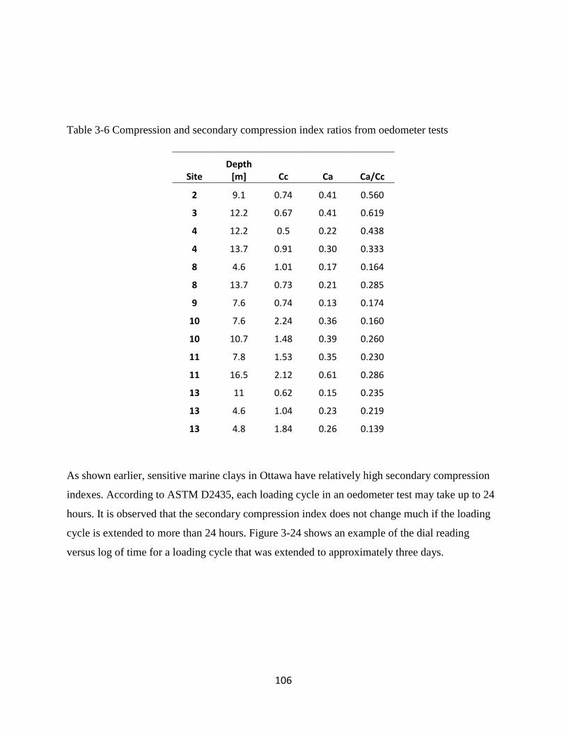
106
Table 3-6 Compression and secondary compression index ratios from oedometer tests
Site Depth
[m] Cc Ca Ca/Cc
2 9.1 0.74 0.41 0.560
3 12.2 0.67 0.41 0.619
4 12.2 0.5 0.22 0.438
4 13.7 0.91 0.30 0.333
8 4.6 1.01 0.17 0.164
8 13.7 0.73 0.21 0.285
9 7.6 0.74 0.13 0.174
10 7.6 2.24 0.36 0.160
10 10.7 1.48 0.39 0.260
11 7.8 1.53 0.35 0.230
11 16.5 2.12 0.61 0.286
13 11 0.62 0.15 0.235
13 4.6 1.04 0.23 0.219
13 4.8 1.84 0.26 0.139
As shown earlier, sensitive marine clays in Ottawa have relatively high secondary compression
indexes. According to ASTM D2435, each loading cycle in an oedometer test may take up to 24
hours. It is observed that the secondary compression index does not change much if the loading
cycle is extended to more than 24 hours. Figure 3-24 shows an example of the dial reading
versus log of time for a loading cycle that was extended to approximately three days.

107
Figure 3-23 Example of dial reading with time from oedometer tests for samples from Ottawa
3.7 Sensitivity of Marine Clay in Ottawa
According to the Canadian Engineering Foundation Manual (2006), sensitivity that is less than 2
is considered as low sensitivity, 2 to 4 as medium sensitivity, 4 to 8 as high sensitivity, and
higher than 16 as quick clay. Figure 3-25 shows the sensitivity with depth for all of the sites
under study. The blue line seperates the low and medium sensitivity regions. Likewise, the green,
black, and red lines separate medium and high sensitivity, high sensitivity to high-quick, and
high-quick to quick regions respectively. In general, sensitive marine clays in Ottawa occupy all
of the sensitivity regions. Most sites (8 sites) occupy 3 sensitivity regions, 4 sites occupy 4
sensitivity regions, and only 1 site occupies 5 sensitivity regions. All of the sites are extended to
beyond the high sensitivity limit while Site 1 is extended from medium to significantly above the
quick limit.
Yong et al. (1979) studied the effect of amorphous material on the sensitivity of Champlain clays
in St. Alban and Gatineau. Even though the study was performed on clays outside the Ottawa
area, the clay is still a Champlain Sea clay and shares similar characteristics with sensitive
marine clays in Ottawa. Amorphous material may hold water in its pores. Amorphous material is
0.25
0.27
0.29
0.31
0.33
0.35
0.1 1 10 100 1000 10000
Dia
l R
eadin
g
Time (min)
one day three days

108
held by quartz grains through electrostatic attraction bonds when mixed with artificially
synthesized silicon-iron hydroxides (Rousseaux and Warkentin 1976). Another study also
showed that amorphous material is mobile during shearing (McKeyes et al. 1974). Therefore,
bonds are likely the reason for high sensitivity in Champlain Sea clays.
Chemical reactions that affect the Gouy double layer in the clay particles reduce the remolded
strength of the soil and increase the sensitivity (Quigley 1980). It has been determined that there
is a correlation between Ottawa clay sensitivity and the electrokinetic potential (Penner 1965).
Clay minerals affect the sensitivity of clay soils. However, as the clay portion in the soil
decreases, the soil sensitivity becomes rather controlled by the cementation bonds (Moum et al.
1971). Also, higher adsorption of Na and K than Ca and Mg are associated with high sensitivity.
The exchange of Ca, Mg, K with Na can reduce the sensitivity of the clay (Moum et al. 1971).
Amorphous material affects the initial and remolded shear strengths of the soil, and therefore, the
sensitivity (Yong and Sethi 1979). Sensitivity is shown to have a direct correlation with
carbonate content and inverse correlation with salinity (Haynes and Quigley 1978; Quigley and
Bohdanowicz 1979). However, there does not seem to be a correlation between sensitivity and
amorphous material. The salinity of marine clays is between 2 and 4 g/L at the surface layer and
15 g/L at deeper layers with higher values of Na+ than Ca
2+, Mg
2+, and K. These salinity values
are considered to be high; therefore the effects of organic dispersants and bicarbonates are
neutralized. In summary, Quigley (1980) and Taha (2010) indicated that high sensitivity depends
on high electrokinetic potential, sediment concentration, divalent cation adsorption, slow rate of
overburden pressure increase, cementation bonds, high water content or higher than the liquid
limit, and low specific surface of soil particles, amorphous content and smectite content.
The sensitivity value reported by Taha (2010) for a depth of 8 to 12 m is 6 from laboratory
testing. The sensitivity is affected by the salinity concentration. Torrance (1975) found that
increases in the salinity decreases the sensitivity and increases the undrained shear strength of
marine clays. He explained that this behavior is attributed to negative surfaces and positive
charged edges of clay particles. A higher ion concentration from salinity reduces the effect of
repulsion between the edges. This also makes it easier for the formation of bonds between
positively charged edges and the negatively charged surface of clay particles. Taha and Fall

109
(2010) found that when the salinity was increased from 10 to 20 g/l, the sensitivity decreased by
50%.
Penner (1965) studied the sensitivity of sensitive marine clays in Ottawa. He observed an
increase in the sensitivity as a result of the addition of sodium metaphosphate. He attributed this
to an increase in the repulsive forces between the clay particles and expected an increase in the
electrokinetic potential. He found that by washing a remolded sample, this can increase the
electrokinetic potential from 19.7 to 23.2 mV and the sensitivity from 34 to 91. On the other
hand, after washing and adding sodium metaphosphate to a remolded sample, this can increase
the electrokinetic potential from 19.7 to 64.6 mV and the sensitivity from 34 to 2150.
Penner (1965) explained that the increase in sensitivity is due to the remolding which breaks the
van der Waal forces between the clay particles, and the adsorbed sodium metaphosphate
increases the repulsion forces between the particles. As a result, the porewater redistributes itself
by forming a separating layer between the particles. When the soil is left for a few days, the
sodium metaphosphate tends to settle and water collects on the surface of the samples even
though the samples have insitu moisture content. The soil structure becomes denser and the
particles form in a face to face rather than cardhouse arrangement. At low salt concentrations,
the sensitivity is highly variable and can be up to 1000, in pore water with a specific conductivity
of less than 4 ohm-1
cm-1
. However, at higher specific conductivity, the sensitivity does not
exceed 75 as a result of the high flocculation. Penner (1965) also established that the sensitivity
consistently increases with electrokinetic potential. From his published results, it can be seen that
in general, there is an increase in sensitivity with a decrease in the clay percentage and the
surface area. There is also an increase in the sensitivity as the concentrations of Na+ and K
+
increase and concentrations of Ca2+
and Mg2+
decrease (Penner 1965).
Dejong et al. (2011) and Yafrate et al. (2009) reported sensitivity values of 33.3 and 68 for
depths of 4.4 and 8.3 m respectively at Site 6. Lo et al. (1976) divided Site 6 into three principle
layers of 6, 6, and 5 m. They assigned an average sensitivity value for each layer in the range of
20 to 100, 50 to 100, and 20 to 50, respectively. According to Eden and Crawford (1957), the
sensitivity of the Ottawa area is between 20 and 60 which was obtained from five profiles.
Mitchell (1970) reported high sensitivity values from block samples at Site 6 at 100, 500, and
500 for depths of 13.7, 16.1, and 19.0 m respectively. The block sample obtained from sensitive

110
marine clay in Ottawa during a sewer installation by Quigley and Thompson (1966) had a
sensitivity between 10 and 12.
(a) (b)
(c) (d)
0
10
20
30
40
50
60
0 50 100
Dep
th [
m]
Sensitivity
0
2
4
6
8
10
12
14
0 6 12 18
Dep
th [
m]
Sensitivity
0
2
4
6
8
10
12
14
16
0 5 10 15 20
Dep
th [
m]
Sensitivity
0
2
4
6
8
10
12
14
16
18
20
0 5 10 15 20
Dep
th [
m]
Sensitivity

111
(e) (f)
(g) (h)
0
5
10
15
20
25
30
0 5 10 15 20 D
ep
th [
m]
Sensitivity
0
2
4
6
8
10
12
14
16
18
20
0 5 10 15 20
De
pth
[m
]
Sensitivity
0
2
4
6
8
10
12
14
16
18
0 5 10 15 20
Dep
th [
m]
Sensitivity
0
2
4
6
8
10
12
14
0 5 10 15 20
Dep
th [
m]
Sensitivity

112
(i) (j)
(k) (l)
0
1
2
3
4
5
6
7
8
9
10
0 5 10 15 20 D
ep
th [
m]
Sensitivity
0
5
10
15
20
25
30
0 5 10 15 20
Dep
th [
m]
Sensitivity
0
1
2
3
4
5
6
0 5 10 15 20
Dep
th [
m]
Sensitivity
0
5
10
15
20
25
0 5 10 15 20
Dep
th [
m]
Sensitivity

113
(m) (n)
Figure 3-24 Sensitivity with depth for (a) Site 1 (b) Site 2 (c) Site 3 (d) Site 4 (e) Site 5 (f) Site 7
(g) Site 8 (h) Site 9 (i) Site 10 (j) Site 11 (k) Site 12 (l) Site 13 (m) Site 14 (n) Site 15
3.8 Hydraulic Conductivity
The coefficient of permeability is a key geotechnical parameter of soil and significantly
influences or controls several geotechnical engineering problems or mechanisms, such as the
groundwater regime in stratified deposits or near natural and excavated slopes, consolidation of
clay foundations, migration of pollutants from waste disposal facilities, and flow of water
through or around engineered structures (Tavenas et al. 1983). Hence, the coefficients of the
permeability of the sensitive marine clays in the sites studied have been assessed.
The coefficient of permeability was determined from one dimensional consolidation tests in
accordance with ASTM D 2435 by using the following equation (Holtz and Kovacs 1981):
1 2
' '
1 2 1
*1
v wc g e ek
e
where k is the coefficient of permeability, Cv is the coefficient of consolidation determined from
oedometer testing, ρw is the density of water, e1 is the void ratio at the start of the loading stage,
0
1
2
3
4
5
6
7
8
0 10 20 30
Sensitivity
0
1
2
3
4
5
6
7
8
0 5 10 15 20
Dep
th [
m]
Sensitivity
114
e2 is the void ratio at the end of the loading stage, and σ2'-σ1' is the difference in the loading
between the previous and current loading stages.
Figure 3-26 shows the variation of the coefficient of permeability with stress for Site 6 and all of
the other sites. The coefficient of permeability generally decreases with increases in the stress.
However, it can increase then decrease with increases with stress, and the reason is the same as
that of the coefficient of consolidation behaviour with stress. As the stress increases, the soil
structure and the porewater take the load and resist compression. At this point, there is high
hydraulic conductivity as the pores are maintained at the same volume. Eventually, the structure
breaks and causes the rearrangement of the soil structure and reduces the hydraulic conductivity.
The coefficient of permeability ranges between 1.58x10⁻⁸
and 3.5x10⁻⁷
cm/s for Site 6 and
between 5.52x10⁻¹⁰
and 1.09x10⁻⁶
cm/s for all of the other sites. Table 3-7 is a summary of all the
coefficients of consolidation with depth, load increment, and preconsolidation pressure of the test
samples.
A profile of the hydraulic conductivity was supplied by the National Research Council Canada
and reported by Hinchberger and Rowe (1998) for the first stage of the embankment of Site 6.
The profile is graphed as shown in Figure 3-27. The hydraulic conductivity ranges between
0.6x10⁹ and 2.7 x10
9 m/s at a depth of 2.13 to 20.73 m. The hydraulic conductivity does not
follow a specific pattern with depth. However, it is higher at the desiccated surface layer and
after a depth of 20 m as there is a layer of coarser silty clay or sandy clay as reported by Yafrate
and Dejong (2005).

115
(a) (b)
(c) (d)
(e) (f)
(g) (h)
0.0E+00
2.0E-08
4.0E-08
6.0E-08
8.0E-08
1.0E-07
1.2E-07
0 200 400 600 800 1000
Co
eff
icie
nt
of
pe
rmeab
ilit
y a
t d
ep
th
of
2.6
m [
m/s
]
Stress [kPa]
0.0E+00
1.0E-08
2.0E-08
3.0E-08
4.0E-08
5.0E-08
6.0E-08
7.0E-08
0 200 400 600 800 1000
Co
eff
icie
nt
of
pe
rmeab
ilit
y a
t d
ep
th
of
4.1
m [
m/s
]
Stress [kPa]
0.0E+00
2.0E-08
4.0E-08
6.0E-08
8.0E-08
1.0E-07
0 200 400 600 800 1000
Co
eff
icie
nt
of
pe
rmeab
ilit
y a
t d
ep
th
of
6.4
m [
m/s
]
Stress [kPa]
0.0E+00
1.0E-08
2.0E-08
3.0E-08
4.0E-08
5.0E-08
6.0E-08
0 200 400 600 800 1000
Co
eff
icie
nt
of
pe
rmeab
ilit
y a
t d
ep
th
of
8.7
m [
m/s
] Stress [kPa]
0.0E+00
1.0E-08
2.0E-08
3.0E-08
4.0E-08
0 200 400 600 800 1000
Co
eff
icie
nt
of
pe
rmeab
ilit
y a
t d
ep
th
of
12.6
m [
m/s
]
Stress [kPa]
0.0E+00
2.0E-08
4.0E-08
6.0E-08
8.0E-08
1.0E-07
1.2E-07
0 200 400 600 800 1000
Co
eff
icie
nt
of
pe
rmeab
ilit
y a
t d
ep
th
of
14.0
m [
m/s
]
Stress [kPa]
0.0E+00
2.0E-08
4.0E-08
6.0E-08
8.0E-08
0 200 400 600 800 1000
Co
eff
icie
nt
of
pe
rmeab
ilit
y a
t d
ep
th
of
15.5
m [
m/s
]
Stress [kPa]
0.0E+00
1.0E-07
2.0E-07
3.0E-07
4.0E-07
0 200 400 600 800 1000
Co
eff
icie
nt
of
pe
rmeab
ilit
y a
t d
ep
th
of
17.1
m [
m/s
]
Stress [kPa]

116
(i) (j)
(k) (l)
(m) (n)
(o) (p)
0.0E+00
1.0E-07
2.0E-07
3.0E-07
4.0E-07
0 200 400 600 800 1000
Co
eff
icie
nt
of
pe
rmeab
ilit
y a
t d
ep
th
of
18.6
m [
m/s
]
Stress [kPa]
0.0E+00
2.0E-08
4.0E-08
6.0E-08
8.0E-08
1.0E-07
1.2E-07
1.4E-07
0 200 400 600 800 1000
Co
eff
icie
nt
of
pe
rmeab
ilit
y a
t d
ep
th
of
9.1
m s
ite 2
[m
/s]
Stress [kPa]
0.0E+00
5.0E-08
1.0E-07
1.5E-07
2.0E-07
0 200 400 600 800 1000
Co
eff
icie
nt
of
pe
rmeab
ilit
y a
t d
ep
th
of
12.2
m s
ite 3
[m
/s]
Stress [kPa]
0.0E+00
2.0E-08
4.0E-08
6.0E-08
8.0E-08
1.0E-07
1.2E-07
1.4E-07
0 200 400 600 800 1000
Co
eff
icie
nt
of
pe
rmeab
ilit
y a
t d
ep
th
of
12.2
m s
ite 4
[m
/s]
Stress [kPa]
0.0E+00
1.0E-07
2.0E-07
3.0E-07
4.0E-07
5.0E-07
0 200 400 600 800 1000
Co
eff
icie
nt
of
pe
rmeab
ilit
y a
t d
ep
th
of
13.7
m s
ite 4
[m
/s]
Stress [kPa]
0.0E+00
5.0E-08
1.0E-07
1.5E-07
2.0E-07
0 200 400 600 800 1000
Co
eff
icie
nt
of
pe
rmeab
ilit
y a
t d
ep
th
of
13.7
m s
ite 8
[m
/s]
Stress [kPa]
0.0E+00
2.0E-08
4.0E-08
6.0E-08
8.0E-08
0 200 400 600 800 1000
Co
eff
icie
nt
of
pe
rmeab
ilit
y a
t d
ep
th
of
7.6
m s
ite 9
[m
/s]
Stress [kPa]
0.0E+00
5.0E-08
1.0E-07
1.5E-07
2.0E-07
2.5E-07
3.0E-07
0 200 400 600 800 1000
Co
eff
icie
nt
of
pe
rmeab
ilit
y a
t d
ep
th
of
7.6
m s
ite 1
0 [
m/s
]
Stress [kPa]

117
(q) (r)
(s) (t)
(u) (v)
Figure 3-25 Coefficient of permeability with stress from oedometer tests for a depth of (a) 2.6 m
Site 6 (b) 4.1 m Site 6 (c) 6.4 m Site 6 (d) 8.7 m Site 6 (e) 12.6 m Site 6 (f) 14.0 m Site 6 (g) 15.5
m Site 6 (h) 17.1 m Site 6 (i) 18.6 m Site 6 (j) 9.1 m Site 2 (k) 12.2 m Site 3 (l) 12.2 m Site 4 (m)
13.7 m Site 4 (n) 13.7 m Site 8 (o) 7.6 m Site 9 (p) 7.6 m Site 10 (q) 10.7 m Site 10 (r) 7.8 m Site
11 (s) 16.5 m Site 11 (t) 11.0 m Site 13 (u) 4.6 m Site 13 (v) 4.8 m Site 13
0.0E+00
1.0E-07
2.0E-07
3.0E-07
4.0E-07
0 200 400 600 800 1000
Co
eff
icie
nt
of
pe
rmeab
ilit
y a
t d
ep
th
of
10.7
m s
ite 1
0 [
m/s
]
Stress [kPa]
0.0E+00
5.0E-08
1.0E-07
1.5E-07
2.0E-07
0 200 400 600 800 1000
Co
eff
icie
nt
of
pe
rmeab
ilit
y a
t d
ep
th
of
7.8
m s
ite 1
1 [
m/s
]
Stress [kPa]
0.0E+00
1.0E-07
2.0E-07
3.0E-07
4.0E-07
5.0E-07
0 200 400 600 800 1000
Co
eff
icie
nt
of
pe
rmeab
ilit
y a
t d
ep
th
of
16.5
m s
ite 1
1 [
m/s
]
Stress [kPa]
0.0E+00
1.0E-07
2.0E-07
3.0E-07
4.0E-07
0 200 400 600 800 1000
Co
eff
icie
nt
of
pe
rmeab
ilit
y a
t d
ep
th
of
11.0
m s
ite 1
3 [
m/s
] Stress [kPa]
0.0E+00
2.0E-07
4.0E-07
6.0E-07
8.0E-07
1.0E-06
1.2E-06
0 200 400 600 800 1000
Co
eff
icie
nt
of
pe
rmeab
ilit
y a
t d
ep
th
of
4.6
m s
ite 1
3 [
m/s
]
Stress [kPa]
0.0E+00
2.0E-08
4.0E-08
6.0E-08
8.0E-08
1.0E-07
1.2E-07
0 200 400 600 800 1000
Co
eff
icie
nt
of
pe
rmeab
ilit
y a
t d
ep
th
of
4.8
m s
ite 1
3 [
m/s
]
Stress [kPa]

118
Table 3-7 Summary of the coefficient of permeability relative to the stress interval, depth, and
preconsolidation pressure from oedometer tests
Site Depth
[m] Stress [kPa]
Coefficient of permeability [m/sec]
Preconsolidation pressure [kPa]
2 9.1 57.1 1.19E-07 107
2 9.1 112.9 9.54E-08 107
2 9.1 224.3 4.40E-08 107
2 9.1 447.3 2.52E-08 107
2 9.1 893.2 1.20E-08 107
3 12.2 57.0 1.52E-07 115
3 12.2 224.1 4.41E-08 115
3 12.2 446.8 2.33E-08 115
4 12.2 29.2 1.17E-07 210
4 12.2 57.0 1.17E-07 210
4 12.2 892.1 3.45E-08 210
4 13.7 35.5 4.69E-07 247
4 13.7 139.3 2.33E-07 247
4 13.7 554.6 7.10E-08 247
6 2.6 32.0 1.10E-07 53
6 2.6 62.8 5.29E-08 53
6 2.6 93.5 3.29E-08 53
6 2.6 124.3 1.63E-08 53
6 2.6 247.3 4.75E-08 53
6 2.6 490.2 1.58E-08 53
6 2.6 982.3 1.95E-08 53
6 4.1 112.4 6.09E-08 58
6 4.1 223.3 3.50E-08 58
6 4.1 445.3 1.75E-08 58
6 6.4 62.8 9.24E-08 57
6 6.4 128.1 4.20E-08 57
6 6.4 247.3 4.63E-08 57
6 6.4 493.3 3.25E-08 57

119
6 8.7 112.4 5.67E-08 52.5
6 8.7 223.3 4.05E-08 52.5
6 8.7 445.3 2.11E-08 52.5
6 12.6 139.9 3.55E-08 52
6 12.6 278.8 2.76E-08 52
6 14.0 32.0 1.08E-07 61
6 14.0 982.3 2.22E-08 61
6 15.5 139.9 7.59E-08 71
6 15.5 278.8 3.64E-08 71
6 15.5 1077.3 1.89E-08 71
6 17.1 62.8 3.50E-07 81
6 17.1 128.1 4.59E-08 81
6 17.1 247.3 3.13E-08 81
6 17.1 493.3 2.20E-08 81
6 18.6 32.0 2.05E-07 90
6 18.6 124.3 1.28E-07 90
6 18.6 493.3 4.53E-08 90
8 4.6 892.1 2.19E-08 225
8 13.7 35.6 1.45E-07 110
8 13.7 139.5 3.97E-08 110
8 13.7 554.7 3.02E-08 110
9 7.6 56.6 5.29E-08 110
9 7.6 111.9 7.27E-08 110
9 7.6 333.0 1.72E-09 110
10 7.6 35.5 1.42E-07 115
10 7.6 139.3 2.49E-07 115
10 7.6 208.5 1.31E-08 115
10 7.6 277.7 4.24E-09 115
10 10.7 58.1 2.20E-07 115
10 10.7 228.4 3.69E-07 115
10 10.7 455.3 1.98E-08 115
11 7.8 29.8 1.58E-07 115
11 7.8 58.1 1.21E-07 115

120
11 7.8 228.4 3.39E-08 115
11 16.5 36.4 2.33E-07 189
11 16.5 142.9 4.49E-07 189
13 11.0 35.0 4.24E-08 40
13 11.0 69.2 3.20E-08 40
13 11.0 137.5 3.48E-07 40
13 11.0 274.2 1.68E-08 40
13 11.0 410.9 5.52E-10 40
13 4.6 56.7 8.50E-08 115
13 4.6 222.9 1.09E-06 115
13 4.6 444.4 1.32E-08 115
13 4.8 29.1 1.10E-07 113
13 4.8 56.9 2.16E-08 113
13 4.8 112.4 1.95E-08 113
13 4.8 334.3 7.19E-09 113
Figure 3-26 Hydraulic conductivity with depth for Site 6 supplied by the National Research
Council Canada and reported by Hinchberger and Rowe (1998)
0
5
10
15
20
25
0 1 2 3
Dep
th [
m]
Hydraulic Conductivity x10^9 [m/s]

121
3.9 Summary and Conclusion
A compilation and review of the engineering geotechnical properties of sensitive marine clays in
Ottawa have been made. Fifteen site locations well spread out in the urban areas of Ottawa have
been studied to characterize sensitive marine clays. Location maps and site descriptions,
including stratifications, geodetic elevations, and water table depths, are provided. Engineering
characteristics such as index properties, grain size distribution, activity, undrained and remolded
shear strengths, sensitivity, shear wave velocity, preconsolidation pressure, overconsolidation
ratio, compression and recompression indexes, coefficient of consolidation, secondary
compression index, and hydraulic conductivity are studied. The work and results of previous
researchers have been discussed and the value ranges for the said engineering properties have
been suggested. Also, a review and summary on the origin and geological settings, porewater
chemistry (Cl, Su, pH, and salinity), clay structure, laboratory shear strength and deformation,
and field and interface shear strengths and behaviour are presented. The characterization of
marine clays in Ottawa with "sensitivity" is supported by the fact that all of the sites under study
extend to beyond the high sensitivity limit or the quick limit.
It is suggested that the Canadian Foundation Engineering Manual has underestimated the shear
strength of sensitive marine clays in Ottawa. The underestimation is presented as the correlation
between the N60 from the SPTs and the undrained shear strength. The underestimation is also
present in the correlation between site classification and the undrained shear strength. The data
sets available are not conclusive as they are limited in number. Therefore, future research should
consider this issue.
Due to the high sensitivity of marine clays in Ottawa, issues are present in the determination of
the remolded shear strength from field and Nilcon vanes. The rate of rotation is slow for
sensitive marine clays in Ottawa in that the soil is capable of gaining strength during testing on
the vane tip or as rod friction. Future research should consider the studying of the rotation rate of
field vanes in sensitive marine clays in Ottawa. In addition, laboratory vane results are compared
to field vane results for the same site. The former shows misestimation, even after correcting for
the rate of rotation or overburden pressure. Future research should consider the adjusting of the
rate of vane rotation so it is as similar as possible with the field vane rotation rate.

122
It has been observed from this research that a double loading scheme for consolidation testing
increases the accuracy of the determination of the coefficient of consolidation. A double loading
scheme renders the curve closer to the theoretical curves expected by interpretation methods. It is
also observed that pore pressure dissipation tests may render an exaggerated coefficient of
consolidation compared to the values obtained from oedometer testing.
The suggested range for the ratio of the secondary compression index to the compression index
for sensitive marine clays in Ottawa has been underestimated by previous researchers. It is found
from this research that the ratio is higher than the suggested range. A ratio of the recompression
index to the compression index has also been suggested in this research.
It is found that the moisture contents of sensitive marine clays in Ottawa are close to or exceeds
the liquid limits which may contribute to the sensitive behaviour of sensitive marine clays in
Ottawa. These clays fall between the A-line and U-line in the plasticity chart which means they
are somewhere in between lean and fat clays. The activities of these clays fall in general in the
normal and inactive areas of the activity chart. However, one site can have a variety of soil
activities that can fall in all of the active, normal, and inactive zones.
It is also found that there is a wide range of soil cone specific factors for sensitive marine clays
in Ottawa. These factors are affected by the distance from the cone and the vane tests. Therefore,
future research should be conducted to verify the ideal distance or determine the limits on the
distance from the penetrometer location and the reference vane location. Also, these clays exhibit
low penetration resistance and sleeve frictions. For this reason, the penetrometers used on
sensitive marine clays in Ottawa are prone to shifts in readings due to temperature effects.
Acknowledgement
This research was carried out to fulfill the requirements of the IPS NSERC, which is a joint
scholarship program for Athir Nader between the University of Ottawa represented by Prof.
Mamadou Fall and Stantec Consulting Limited represented by Raymond Hache.
123
3.10 References
Andrews, J. T. (1972). Post-glacial rebound. The National Atlas of Canada, Canada Department
of Energy, Mines and Resources 35–36.
Bell, F. G. (2000). Engineering properties of soils and rocks. Blackwell Science Ltd., London,
UK.
Bentley, P. (1980). Significance of amorphous material relative to sensitivity in some Champlain
c1ays 1.
Bozozuk, M. (1971). Effect of sampling, size, and storage on test results for marine clay.
American Society of Testing Material Spec. Tech. Publication 483:121–131.
Brydon, J. E., Patry, L. M. (1961). Mineralogy of Champlain Sea sediments and a Rideau clay
soil profile. Canadian journal of soil science 41:169–181.
Campanella, R. G., Sully, J. P., Robertson, P. (1988). Interpretation of piezocone soundingd in
Clay - a case history. Institution of Civil Engineers, Sym. on Penetration Testing in the U.K.,
Thomas Telford, London.
Chan, H. T., Kenney, T. (1973). Laboratory investigation of permeability ratio of New Liskeard
varved soil. Canadian geotechnical journal 10:453–472.
Conlon, R. J. (1966). Lanslides on the Toulnustouc River, Quebec. Canadian geotechnical
journal 3:113–144.
Crawford, C. B. (1961). The influence of strain on shearing resistance of sensitive clay. ASTM
61:1250–65.
Crawford, C. B. (1968). Quick clays of eastern Canada. Engineering Geology 2(4):239–265.
Crawford, C. B., Eden, W. J. (1965). A comparison of laboratory results with in-situ properties
of Leda Clay. 6th Int. Conf. SM and FE 1:31–35.
Cronin, T. M. (1977). Late-Wisconsin marine environments of the Champlain Valley.
Quarternary Research, New York, Quebec 7:238–253.

124
Dam, T. K. L., Yamane, N., Hanzawa, H. (1997). Direct shear test results on four soft marine
clays. Proc. of Int. Symp. on The Characterization of soft Marine Clays 229–240. Yokosuka,
Japan: A.A Balkema.
Dayal, S. (1970). Removal of swelling clay minerals from Leda clay and influence on the
permeability. The University of Western Ontario.
Dejong, J. T., Asce, M., Yafrate, N. J., Degroot, D. J. (2011). Evaluation of Undrained Shear
Strength Using Full-Flow Penetrometers 14–26.
DeJong, J. T., Westgate, Z. J. (2005). Role of overconsolidation on sand-geomembrane.
Geotextile and Geomembrane 23:486–512.
DeJonge, J. T., Westgateb, Z. J. (2009). Role of initial state, material properties and cinfinement
condition on local and global soil-structure interface behaviour. Journal of Geotechnical and
Geoenvironmental Engineering 135(11):1646–1660.
Delage, P., Lefebvre, G. (1984). Study of the structure of a sensitive Champlain clay and of its
evolution during consolidation. Canadian Geotechncial Journal 21(1):21–35.
Donovan, J. J., Lajoie, G. (1979). Geotechnical implication of diagenetic iron sulphide
formation in Champlain Sea sediments. Canadian Journal of Earth Sciences 16:575–584.
Eden, W. J., Crawford, C. (1957). Geotechnical properties of Leda Clay in the Ottawa area.
Research Paper No. 37 Of The Division Of Building Research Ottawa, NRC 4383.
Elson, J. A. (1967). Geology of glacial lake Agassiz. University of Manitopa Press, Winnipeg
36–95.
Fleming, I., Sharma, J. S., Jogi, M. B. (2006). Shear strength of geomembrane-soil interface
under unsaturated conditions. Geotextiles and Geomembranes 24:274-284.
Gadd, N. R. (1975). Geology of Leda clay. Mass Wasting, 4th Guelph Symposium on
Geomorphology 137–151.
Gilbert, R. (1975). Sedimentation in Lillooet lake, British Columbia. Canadian journal of earth
science 12:1697–1711.

125
Gillott, J. E. (1970). Fabric of Leda clay investigated by optical, electron-optical and X-ray
diffraction methods. Engineering Geology 4:133–153.
Hamid, T., Miller, G. (2009). Shear strength of unsaturated soil interfaces. Canadian
Geotechnical Journal 46:595–606.
Haynes, J. E., Quigley, R. M. (1978). Framboids in Champlain Sea sediments. Canadian Journal
of Earth Sciences 15:464–465.
Hendershot, W. H., Carson, M. A. (1978). Changes in the plasticity of a sample of Champlain
clay after selective chemical dissolution to remove amorphous material. Canadian geotechnical
journal 15:609–616.
Hillaire-Marcel, M. C. (1979). Les mers post-glaciaires du Quebec: quelques aspects. Published
these de doctorat d’Etat es Sciences Naturelles, 2 vols.
Hinchberger, S. D., Rowe, R. K. (1998). Modelling the rate-sensitive characteristics of the
Gloucester foundation soil. Canadian Geotechnical Journal 35:769–789.
Holtz, R. D., Kovacs, W. D. (1981). An introduction to geotechnical engineering. Prentice-Hall,
Inc , New Jersey.
Jarrett, P. M. (1967). Time-dependant consolidation of a sensitive clay. Materials Research and
Standards 7:300–304.
Karrow, P. F., Anderson, T. W., Clake, A. H., Delorme, L. D. (1975). Stratigraphy, paleontology
and age of Lake Algonquin sediments in southwestern Ontario, Canada. Quaternary Research
5:49–87.
Kenney, T. C. (1964). Sea level movements and the Boston, Nicolet, Ottawa and Oslo.
Geotechnique 14:203–230.
Kenney, T. C. (1968). A review of recent research on strength and consolidation of soft sensitive
clays. Canadian geotechnical journal 5:97–119.

126
Kenney, I. C., Janbu, N., Jorstad, F., Kjaernsli, B. (1976). Formation and geotechnical
characteristics of glacil-lake varved soils. Norwegian Geotechnical Institute Publication, (In
Laurits Bjerrum Memorial Volume) 15–39.
Konrad, J. M., Law, K. (1987). Undrained Shear Strength From piezocone tests. Canadian
geotechnical journal 24(3):392–405.
Ladd, C. C. (1975). Discussion: Measurement of in situ shear strength. Proceedings In Situ
Measurements ASCE Vol. II:153–160.
Landon, M. M., Low, H. E., Randolph, M. F., DeGroot, D. J. (2011). Geotechnical
characterisation and engineering properties of Burswood clay. Géotechnique 61(7):575–591.
doi:10.1680/geot.9.P.035
Larsson, R. (1980). Undrained shear strength. Canadian Geotechncial Journal 17(4):591–602.
Laventure, R. S., Warkentin, B. P. (1965). Chemical properties of Champlain Sea sediments.
Canadian Geotechnical Journal 2:299–308.
Law, K. T., Bozozuk, H. (1988). Engineering problems in Leda Clay. In Proceedings of the
International Conference (ICEPRS 88) on “Engineering Problems of Regional Soils” 775–792,
Beijing, China.
Leroueil, S. (1999). Geotechnical characteristics of eastern Canada clays. In Proceedings of the
International Symposium on the characterization of soft marine clays 3–32. A.A Balkema,
Yokosuka, Japan.
Leroueil, S., Tavenas, F., Samson, L., Morin, P. (1983). preconsolidation pressure of Champlain
clay. Canadian geotechnical journal 20:803–816.
Leroueil, S., Sampson, L., Bozozuk, M. (1983). Laboratory and field determination of
preconsolidation pressures at Gloucester. Canadian Geotechnical Journal 20:477–490.
Lo, K. Y., Bozozuk, M., Law, K. T. (1976). Settlement analysis of the Gloucester test fill.
Canadian Geotechnical Journal, 13:339.

127
Lo, K. Y., Morin, J. P. (1972). Strength anisotropy and time effects of two sensitive clays.
Canadian Geotechnical Journal 9(3):261–277.
Lo, K. Y., Ho, K. S., Inculet, I. (1991). Field test of electroosmotic strengthening of soft sensitive
clay. Canadian Geotechncial Journal 28:74–83.
May, R. W. (1977). Facies model for sedimentation in the glaciolacustrine environment. Boreas,
6:175–180.
McKeyes, E., Sethi, A. J., Yong, R. N. (1974). Amorphous coatings on particles of sensitive clay
soils. Clays and Clay Minerals 22:427–433.
Mitchell, R. J. (1970). On the yielding and mechanical strength of Leda clays. Canadian
Geotechncial Journal 7:297.
Morgenstern, N. R. (1967). submarine slumping and the initiation of turbidity currents.
University of Illinois Press In Marine geotechnique 189–220.
Moum, J., Loken, T., Torrance, J. K. (1968). Stabilization of quick clay by salt wells. Norway
Geotechnical Institute Pub1 8:81.
Moum, J., Loken, T., Torrance, J. K. (1971). A geochemical investigation of the sensitivity of a
normally consolidated clay from Drammen, Norway. Geotechnique 21:329–340.
Moum, J., Loken, T., Torrance, J. K. (1972). A geochemical investigation of the sensitivity of a
normally consolidated clay from Drammen. Geotechnique 22:675–676.
Penner, E. (1965). A STUDY OF SENSITIVITY IN LEDA CLAY. Canadian Journal of Earth
Sciences 2:8592.
Quigley, R. M. (1980). Geology , mineralogy , and geochemistry of Canadian soft soils : a
geotechnical perspective1 Distribution of Soft Soils in Canada. Canadian Geotechnical Journal
17:261–285.
Quigley, R. M., Ogunbadejo, T. A. (1972). Clay layer fabric abd oedometer consolidation of a
soft varved clay. Canadian Geotechnical Journal 9:165–175.

128
Quigley, R. M., Bohdanowicz, A. (1979). Supplimentary research, piezometric water conditions,
preconsolidation, and isotope analyses on Leda clay from deep boreholes, Addendum report to
the Ontario Ministry of Natural Resources, Hawkesbury, Ontario.
Quigley, R. M., Thompson, C. D. (1966). The Fabric of Anisotropically Consolidated Sensitive
Marine Clay. Canadian Geotechnical Journal 3(2):61–73.
Rasmussen, K. K. (2012). An Investigation Of Monotonic And Cyclic Behaviour Of Leda Clay.
The University of Western Ontario.
Rousseaux, J. M., Warkentin, B. (1976). Surface properties and forces holding water in
allophane soils. Soil Science Society of America 40:446–451.
Skempton, A. (1953). The colloidal activity of clays. 3rd International Conference on Soil
Mechanics and Foundation Engineering 1:57–61.
Soderman, L. G., Quigley, R. M. (1965). Geotechnical properties of three Ontario clays.
Canadian geotechnical journal 2:167–189.
Syvirski, J. P. (1978). Sedimentological advances concerning the flocculation and zooplankton
pelletization of suspended sediment in Howe Souls, British Columbia: A fjord recieving glacial
meltwater. Ph.D. thesis, University of British Columbia, Vancouver, B.C., 291.
Syviski, J. P., Murray, j. W. (1980). Particle interaction in fjord suspended sediment. Marine
Geology.
Syvitski, J. P., Farmer, D., Freeland, H. J. (1980). Flocculation, agglomeration and zooplankton
pelletization of suspended sediment in a fjord receiving glacial meltwater. NATO Conference, In
Fjordo 616–625.
Taha, A. M., (2010). Interface Shear Behavior of Sensitive Marine Clays -Leda Clay. M.A.Sc.
Thesis, Department of Civil Engineering, The University of Ottawa.
Taha, A. M., Fall, M., (2010). Shear Behavior of Sensitive Marine Clays -Concrete Interface. .
Journal of Geotechnical and Geo-environmental Engineering 139(4):644–650

129
Tavenas, F., Jean, P., Leblond, P., Leroueil, S. (1983). The permeability of natural soft clays.
Part II: Permeability characteristics. Canadian Geotechnical Journal 20:645-660.
Taylor, D. W. (1948). Fundamentals of Soil Mechanics. John Wiley and Sons, Inc, New York.
Torrance, J. (1975). On the role of chemistry in the development and behaviour of the sensitive
marine clays of Canada and Scandinavia. Canadian Geotechnical Journal 12:326–335.
Townsend, D. L., Sangrey, D. A., Walker, L. K. (1969). The brittle behaviour of naturally
cemented soils. Proceedings, 7th International Conference on Soil Mechanics and Foundation
Engineering, Mexico City 2:411–417.
Tsubakihara, Y., Kisheda, H. (1993). Frictional behaviour between normally consolidated clay
and steel by two direct shear type apparatus. Soils Foundation 33:1–13.
Van Zelst, T. W. (1948). An investigation of the factors of affecting laboratory consolidation of
clay. Proceedings of the second International Conference on Soil Mechanics and Foundation
Engineering 52–61. Rotterdam.
Walker. L. K., Raymond, G. P. (1968). The prediction of consolidation rates in a cemented clay.
Canadian Geotechncial Journal 4:192–216.
Yafrate, N. J., Dejong, J. T. (2005). Considerations in evaluating the remoulded undrained shear
strength from full flow penetrometer cycling 991–998.
Yafrate, N., Asce, S. M., Dejong, J., Asce, M., Degroot, D., Randolph, M. (2009). Evaluation of
Remolded Shear Strength and Sensitivity of Soft Clay Using Full-Flow Penetrometers 1179–
1189.
Yafrate, N., Nicholas, J., Dejong, J. T. (2006). Interpretation of Sensitivity and Remolded
Undrained Shear Strength with Full Flow Penetrometers 1–6.
Yong, R. N., Sethi, A. J., LaRochelle, P. (1979). Significance of amorphous material relative to
sensitivity in some Champlain clays. Canadian Geotechnical Journal 16(3):511–520.
doi:10.1139/t79-057

130
Yong, R. N., Sethi, A. J. (1979). Significance of amorphous material relative to sensitivity in
some champalin clays. Canadian geotechnical journal 16:511–520.

131
Chapter 4: Technical Paper II - Characterization of Sensitive
Marine Clays by Using Cone and Ball Penetrometers – Examples of
Clays in Eastern Canada
N. Athir, M. Fall, R. Hache
Abstract
Soundings made by using the cone penetration test in sensitive marine clay in Ottawa (Canada)
have been problematic. Negative readings have been recorded. The incorrect estimation of the
engineering characteristics of Ottawa clays has been noted. The effect of temperature on the
output of penetrometer load cell is suspected as the reason for the negative drift in soundings and
erroneous estimations of engineering characteristics. Also, focused research is needed to verify
existing correlations and empirical factors between the cone penetration test and engineering
characteristics of Ottawa clays. These are the reasons for carrying out this research work.
Temperature effects have become a significant factor in countries with radical temperature
changes, such as Canada. Three types of penetrometer tips have been used at the Canadian
Geotechnical Research Site No. 1. The tips used are a 36 mm cone, and 40 mm and 113 mm
balls. Nilcon field vane testing has also been carried out in the site to determine the undrained
shear strength and sensitivity (the ratio of the initial undrained shear strength to the remolded
undrained shear strength) from the penetrometer soundings. Undisturbed samples are collected to
obtain the engineering characteristics by laboratory testing. Laboratory testing on penetrometer
equipment is performed to verify the effects of temperature on the soundings. It is found that
temperature changes affect the penetrometer soundings. Temperature effects can cause drifting
as indicated by negative tip stress or sleeve friction in soft or low resistance clays. Therefore,
temperature effects may increase the errors in the estimation of the engineering characteristics of
Ottawa clays. It has also been found that correlations may or may not apply well to Ottawa
sensitive marine clay. Temperature corrections could be applied to the penetrometer soundings.
From this research, correlations and empirical factors between penetrometers and engineering
characteristics are verified for Ottawa sensitive marine clays.

132
Keywords
Ball penetrometers, CPT, Temperature, Gloucester, Ottawa, Leda Clay, Sensitive Marine Clay
4.1 Introduction
Various types of penetrometers have been increasingly used to estimate the engineering design
parameters of soils. The different possibilities of measuring profiles have given penetrometers
advantages over other conventional means of field testing, such as standard penetration and vane
shear testing. Different penetrometer sizes and tip shapes have been used for the purpose of
improving the estimations of engineering soil characteristics. Cone, ball, and T-bar
penetrometers are the most commonly used. Cone tips are considered the conventional
penetrometer tip shape. The literature is rich with work carried out on the correlations between
cone penetration tests (CPTs) and soil properties in geotechnical engineering, such as shear
strength, sensitivity, grain size, and consolidation history (Battaglio et al. 1981; Lunne and
Kleven 1981; Rad and Lunne 1986 and 1988; La Rochelle et al. 1988; Marsland and Powell
1988; Powell and Quarterman 1988; Robertson and Campanella 1988; Suzuki et al. 1995;
Karlsrud et al. 1996; Lunne et al. 1997; Low et al. 2010). However, although these correlations
have been verified with a variety of soils, not all types of soils have been investigated. These
correlations have not been specifically verified with sensitive marine clays in Ottawa. The
verification and modification of these correlations with local experience (Lunne et al. 1997) are
recommended. Ball and T-bar penetrometers (full-flow penetrometers) were initially used for the
centrifugation of samples (Stewart and Randolph 2001). Later, the use of full-flow penetrometers
was extended to estimating the undrained and remolded shear strength and sensitivity of clays
due to the remolding effects from the plastic behaviour of soil around the tip and probe.
Furthermore, as full-flow penetrometers have larger projected areas of the tip in comparison to
cone penetrometers, they have been used in extremely soft soils. Full-flow penetrometers are less
influenced by overburden stress which makes them more accurate in the estimation of undrained
shear strength than cone penetrometers (DeJong et al. 2010). However, our understanding of the
use of ball penetrometers for the purpose of characterizing the geotechnical properties of
sensitive marine clays, particularly those in Ottawa, is still limited. Research is needed to address
this issue.

133
Temperature effects are expected to be the cause of the erroneous estimations of engineering
characteristics from penetrometer tests. Negative tip resistance and sleeve friction have been
found by Boylan and Long (2007). Radical temperature changes may be experienced by
penetrometer equipment. Temperature records from The Weather Network have shown that the
average high and low temperatures in Ottawa are 26.4C and -14.8C in the summer and winter
respectively while the ground temperature is constant between 8C and 9C at a depth of around
6 m throughout the year. Therefore, there is a temperature change of up to 18C from the surface
to a depth of about 6 m that may cause a shift in penetrometer readings. Thus, there is the need to
better understand the effect of temperature changes on penetrometer testing for Ottawa soils.
Moreover, research is needed to verify existing correlations and empirical factors between CPTs
and the engineering characteristics of marine clays in Ottawa. Therefore, this research aims to
address the aforementioned needs.
The main objectives of this research are: (i) to characterize the engineering properties of
sensitive marine clays in Ottawa (located at the Canadian Geotechnical Research Site No. 1) by
using penetrometers; (ii) to understand the effect of temperature changes on penetrometer testing
in soils in Ottawa; (iii) to assess existing correlations and empirical factors between CPTs and
engineering properties of marine clays in Ottawa, with the view to developing guidelines for
practicing engineers who work with these sensitive marine soils and other similar soils
worldwide.
For the purpose of this research, field and laboratory tests are performed at the Canadian
Geotechnical Research Site No. 1. The field tests performed include two CPTs with a cone tip
that is 36 mm in diameter (CPT-1 & CPT-2), two ball penetrometer tests (BPTs) with a tip that
has a 40 mm ball (BPT-1 & BPT-2), and one set of Nilcon field vane tests. Undisturbed samples
are also collected and water table monitoring wells are installed. The variables in the laboratory
tests that are investigated include unit weight, moisture content, plasticity limits, salinity and
specific gravities and consolidation parameters. Furthermore, the grain size distribution of the
samples is determined in the laboratory. Laboratory testing on temperature change is also carried
out on the penetrometer to verify the effects of temperature changes on the penetrometer
readings.

134
4.2 Site description
The Canadian Geotechnical Research Site No. 1 is a representative site for sensitive marine clay
deposits in Ottawa (Eastern Canada). Previous researchers have performed field testing on the
site, such as cone penetration, full-flow penetrometer, vane, and laboratory tests, to examine the
plasticity properties by using oedometers and through triaxial testing (Lo et al. 1976; Yafrate and
Delong 2006; Yafrate et al. 2009; DeJong et al. 2011). Therefore, there is an abundance of
reference information available in the literature about the site.
4.2.1 Geographical location
The Canadian Geotechnical Research Site No. 1 (Figure 4-1) is located in south-east Ottawa on
an average geodetic elevation of 80.9 m, northing of 5016868.8, and easting of 459267.3
according to the Transverse Mercator projection system (NAD_1983_MTM_8 projected
coordinate system).
Figure 4-1 Geographical location of the Canadian Geotechnical Research Site No. 1

135
4.2.2 Geological characteristics
At the end of the glacial period, areas of Canada were depressed for hundreds of meters. After
the glacial retreat, marine waters flooded the St. Lawrence River valley, thus forming the
Champlain Sea (Crawford 1968). The Champlain Sea existed between 12000 and 8000 B.P.
(Karrow 1961). During that period of time, there was an isostatic adjustment which resulted in
the land rising as much as 230 m (Kenney 1964). The highest sea level was recorded near the
Ottawa area at about 226 m above the present sea level (Johnston 1917). Streams that entered the
sea from the north side as a result of the ice retreat deposited fine materials and formed deltas.
Later, when the sea level rose, these deposits eroded and were redeposited back into the sea
(Karrow 1961). Studies have mentioned that marine deposits were deposited into fresh water as
floods invaded the sea from the great lakes. This assumption is based on the existence of non-
oxidized, non-calcareous, and non-fossiliferous clay layers that lie on unoxidized calcareous
fossiliferous clay layers (Gadd 1962). This also explains the drop in salt content in Ottawa clays
(Crawford and Eden 1965).
The stratigraphy of the Canadian Geotechnical Research Site No. 1 generally consists of a clay
layer that is 20 m in thickness under which lies bedrock or refusal layer that has a depth of about
22 m or a geodetic elevation of 59 m. The clay layer includes a 2 m crust near the ground
surface.
Yafrate and DeLong (2006) provided a geological profile of the site. According to their profile,
there is a crust layer that is approximately 2 m in depth, a meter of brown silty clay layer, 4.5 m
of grey silty clay, 7 m of grey clay, and less than a meter of grey silty sand. The difference in the
geotechnical profile description between the literature and this research may be due to the
location of the field investigation. The field investigation performed for this study is near the
gate and the sign of the site location while the location of field investigation carried out by
previous researchers has not been clearly indicated.

136
4.3 Experimental Programs and Soil Characterization
4.3.1 Field testing programs
4.3.1.1 CPT Tests
Two CPTs were performed in accordance with ASTM D 5778. The tip stress, sleeve friction,
porewater pressure, and temperature were recorded in each sounding. An average penetration
rate of 20 mm/sec was used. The diameter of the cone tip is 36 mm and the push rods have the
same diameter. Porewater pressure was measured at Position 2 which allows for tip stress
correction.
4.3.1.2 Ball Penetrometers
Soundings were performed by carrying out two BPTs, one with two penetrometers that have a 40
mm ball, and one with a penetrometer that has a 113 mm ball. A penetration rate of 20 mm/s was
used for the latter while a rate of 12 mm/sec (0.2-0.3 times the diameter per second) was used for
the former as recommended by DeJong et al. (2010).
4.3.1.3 Field Vane Shear Tests
A standard electric field vane was used (ASTM D2573) with a tapered lower end that has a
dimension of 130 x 65 mm. A rate of 0.1 deg./s was used and ten rapid rotations were performed
before the remolded shear strength was determined. A series of tests on undrained and remolded
shear strength at a 1 m interval were performed.
4.3.1.4 Drilling and sampling
Undisturbed samples were collected for laboratory testing in accordance with ASTM D 1587 for
thin-walled tube sampling. Shelby tubes that are 0.0762 m (3 in) in diameter and 0.762 m (2.5 ft)
in length were used. The tubes meet the criterion for a 1% inside clearance ratio as specified by
ASTM standards. A piston sampler was used to ensure the quality of sampling and avoid the
material from falling out of the tube due to suction. The boreholes were pre-augered in advance
to a depth of 1.5 m (5 ft) and sampling started at the same depth at intervals of 0.762 m (2.5 ft)
and spacing of 0.0015 m (0.5 ft). The piston was kept in a locked position at the bottom of the
tube while it was being pushed to the desired depth. Then, the piston was fixed at a specific

137
depth and only the tube was pushed to a distance of 0.43 m rather than 0.762 m in order to
prevent the disturbance of the sample by the piston head. While pulling the tube up to the
surface, the piston was locked at the top of the tube to provide pressure from suction which
would prevent any material from falling out of the tube. Also, a distance of 0.15 m (0.5 ft) was
placed between samples to minimize disturbance.
4.3.1.5 Wells installation
Multi-level monitoring wells were installed in accordance with ASTM D 5092 to monitor the
water level or porewater pressure at two different depths. Temporary auger casing was provided
to a geodetic elevation of 59 m. Screens (1.5 m in length) were installed at elevations of 59.3
and 74.5 m, and surrounded with clean sand up to 0.3 m above the screen level. Above the sand,
a 1 m seal of bentonite was situated to prevent water from penetrating into the screen from the
higher layers. Grout was used around the riser up to 1 m below the surface where 1 m of
bentonite was used to seal the well from the surface. A 0.5 m stick up with protective steel casing
was used. Readings of the water level in the two wells started the next day from the installation
time on an average of once a day for ten days and once a month afterwards, as shown in figure 4-
2. A general increase in the water level in the two wells can be noted towards the winter months.
This is probably a result of the increased overburden stress due to snow accumulation. Porewater
pressure readings at Position 2 (u2) were measured by the cone penetrometer, and penetrometers
with 40 and 113 mm balls. The readings are shown in figure 4-3 with hydrostatic pore water
pressure. As expected, there is a reduction in the excess pore water pressure as the tip projected
area increases. Furthermore, u2 sensitivity to stratification and identification of the layer
boundaries is reduced as the tip projected area increases.

138
Figure 4-2 Water table geodetic elevations with dates from the multilevel monitoring wells
Figure 4-3 Porewater pressure readings from cone, 40 mm ball, and 113 mm ball tips and
hydrostatic porewater pressure with geodetic elevations, CPT-1 and CPT-2 are porewater
pressure readings from cone tip tests 1 and 2, 40-ball-1 and 40-ball-2 are porewater pressure
readings from 40 mm ball tip tests 1 and 2, 113-ball is porewater pressure readings from 113 mm
ball tip test, HPP is hydrostatic porewater pressure readings from monitoring wells readings
58
64
70
76
82
29-A
ug-1
2
23-S
ep-1
2
18-O
ct-
12
12-N
ov-1
2
7-D
ec-1
2
1-J
an-1
3
26-J
an-1
3
20-F
eb-1
3
17-M
ar-
13
11-A
pr-
13
6-M
ay-1
3
31-M
ay-1
3
25-J
un-1
3
Geo
deti
c E
lev
ati
on
[m
]
59.3 m
74.5 m
55
60
65
70
75
80
0 200 400 600 800
Geo
deti
c E
lev
ati
on
[m
]
Porewater Pressure [kPa]
CPT-1 CPT-2 40-ball-1 40-ball-2 113-ball HPP

139
4.3.1.6 Geodetic Elevations and coordinates
Table 4-1 is a summary of the geodetic elevations, easting, and northing of all field tests.
Table 4-1 Geodetic surface elevations, easting, and northing of field testing points
4.3.2 Laboratory testing programs and soil characterization
4.3.2.1 Unit weight, moisture content, and specific gravity
Unit weight, moisture content, and specific gravity were determined for 11 samples collected
from the field in accordance with ASTM D 7263, ASTM D 2216, and ASTM D 854 respectively
(Figure 4-4). The displacement method was used to determine the unit weight, while specific
gravity was determined by using oven-dried specimens. The site is characterized by three layers:
a top layer of 0.75 to 1.2 m, an intermediate layer of 19 m, and a bottom layer of 1 m down to a
geodetic elevation of 59 m (21 m in depth). The top, intermediate and bottom layers have a unit
weight of 22.8 kN/m3, 16 kN/m
3 and 19.1 kN/m
3 respectively. The moisture content follows a
pattern that is similar to the unit weight, in which the top, intermediate and bottom layers have an
average moisture content of 11.4%, 68.3% (range from 46% to 89.2%), and 37%, respectively
The specific gravity has a narrow range from 2.74 to 2.79 with the lowest value recorded at the
top layer.
Label
Geodetic Surface
Elevation [m] Northing Easting Description
BPT-1 80.801 5016876.239 459278.466 40 mm ball
BPT-2 80.655 5016874.562 459286.533 40 mm ball
CPT-1 80.449 5016861.039 459294.614 36.6 mm cone
CPT-2 80.899 5016869.712 459275.890 36.6 mm cone
Bore
Hole 80.670 5016865.117 459281.522
Undisturbed Samples and
multi-level Monitoring
Wells
Field
Vane 80.735 5016870.089 459292.803 Nilcon Field Vane
BPT-3 80.907 5016869.305 459279.829 113 mm ball

140
Figure 4-4 (a) unit weight with geodetic elevations (b) moisture content with geodetic elevations
(c) specific gravity with geodetic elevations
4.3.2.2 Grain size distribution and soil index properties
Grain size distribution and plasticity limits were determined in accordance with ASTM D 422
and ASTM D 4318 respectively. The top layer is a sandy silt layer with 16.9% clay and 2.6%
gravel. Under the top layer is a deep silty clay layer up to 20 m thick. The fines content ranges
from more than 80% to less than 80% clay particles. This type of deposition has been reported by
Leroueil (1999) as a result of summer silty and winter clayey depositions, but in terms of smaller
couplets that are a few centimeters in thickness. With respect to geodetic elevation, the silty
deposition layer ranges from 76 to 78 m, 63.5 to 67.5 m, and 59 to 61.5 m where CPT refusal
takes place at 59 m, with transition layers of 1.5 to 3 m, respectively. Clayey deposition layers
vary in thickness of 2 to 8.5 m. The moisture content parallels with the layering in that there is a
decrease in the former when there is an increase in the silt content as in geodetic elevations of
60.5 and 66.5 m. There is also an increase in the unit weight at the same elevations to 17.7
kN/m3 and 19.1 kN/m
3 respectively, while specific gravity shows a decrease at these depths
(Figure 4-4 and 4-5). The plastic limits, liquid limits, and plasticity index range between 26.3%
to 59.9%, 14.8% to 37%, and 11.5% to 28.1% respectively (Figure 4-6). DeJong et al. (2011)
55
60
65
70
75
80
10 15 20 25
Geo
deti
c E
lev
ati
on
[m
]
Unit Weight [kN/m]
0.0 50.0 100.0
Moisture Content [%]
2.7 2.75 2.8
Specific Gravity

141
reported higher values at two depths. He reported the plastic limit, liquid limit, and plasticity
index to be 27, 71, and 44 for a depth of 4.4 m, and 28, 62, and 34 for a depth of 8.3 m
respectively.
Figure 4-5 (a) percentage particles size with geodetic elevations (colloids <0.001 mm, clay
0.001-0.005 mm, silt 0.005-0.075, sand 0.075-0.04.75 mm, gravel 4.75-75 mm) (b) plasticity
index with geodetic elevations (c) moisture content with geodetic elevations
60
65
70
75
80
0 20 40 60 80 100
Geo
deti
c E
lev
ati
on
[m
]
Percentage Passing [%]
Colloids Clay
Silt
Sand
Gravel
<80% clay layer
>80% clay layer
>80% clay layer
>80% clay layer
<80% clay layer
10 20 30
Plasticity Index [%]
0.0 50.0 100.0
Moisture Content [%]

142
Figure 4-6 Moisture contents, plastic limits, and liquid limits with geodetic elevations, PL is the
plastic limits, LL is the liquid limit, MC is the moisture content
4.3.2.3 Preconsolidation Pressure
One-dimensional consolidation tests were performed in accordance with ASTM D 2435.
Preconsolidation pressure and OCR values are shown with geodetic elevation in Figure 4-7. It is
evident that there is a general increase in the preconsolidation pressure and decrease in the OCR
with depth. The soil is lightly overconsolidated at an elevation of 75 to 80 m, and normally
consolidated at an elevation lower than 75 m. DeJong et al. (2011) reported that the soil in their
investigation is overconsolidated to 1.8 at a depth of 4.4 m and 1.5 at a depth of 8.3 m.
60
65
70
75
80
10 30 50 70 90
Geo
deti
c E
lev
ati
on
[m
]
Moisture Content [%]
PL
LL
MC

143
Figure 4-7 (a) preconsolidation pressure with geodetic elevations (b) overconsolidation ratio with
geodetic elevations
4.3.2.4 Porewater Chemistry
The pore water chemistry was analyzed for sodium, potassium, magnesium, and calcium cations
and chloride anions (Na+, K
+, Mg
+2, Ca
+2, and Cl
-). Chloride anions seem to parallel the
sensitivity and plasticity index. There are noticeable increases in the chloride concentrations at
elevations of 63.5, 70 and 76.5 m, and similar increases in the sensitivity (figure 4-14) and
plasticity limits (figure 4-18) at similar depths. There is also similar behavior in the sodium,
magnesium, and potassium profiles, but with less clarity than in the chloride profile. Therefore,
the relation between chloride, sodium, magnesium, and potassium on the one hand and
sensitivity and plasticity on the other hand is positive. In other words, there seems to be an
increase in the sensitivity and plasticity as chloride, sodium, magnesium, and potassium
concentrations increase. Calcium does not seem to be related to the sensitivity or plasticity
(figure 4-8).
60
65
70
75
80
50 60 70 80 90 100
Geo
deti
c E
lev
ati
on
[m
] Preconsolidation Pressure
[kPa] 0.0 1.0 2.0
Overconsolidation Ratio

144
Figure 4-8 (a) chloride Cl anions (b) calcium Ca cations (c) magnesium Mg cations (d)
potassium K cations (e) sodium Na cations with geodetic elevations
4.3.2.5 Cone Equipment Calibration and Temperature Effects
The results gathered by CPTs on sensitive marine clays have been problematic. Temperature
effects may induce negative readings and/or increases or decreases in tip resistance, sleeve
friction, and porewater pressure readings. Temperature effects may also cause a shift in the
baseline reading of the soundings. According to ASTM D 5778, baseline readings must take
place before and after each penetrometer sounding where the equipment is vertically and freely
hung with zero loads. The initial baseline reading is used as a reference or zero transducer
reading while the final baseline reading with reference to the initial baseline reading is used to
verify the reliability of the data or determine the baseline drift due to temperature or other
effects. According to The Weather Network statistics for Ottawa, an average high temperature of
26.4C is recorded for July, and an average low temperature of -14.8C is recorded for January.
According to Williams and Gold (1976), at a depth of 5 to 6 m, the ground temperature is
constant at 8C to 9C, and changes about 1C for every 50 m in depth due to the geothermal
heat from the centre of the earth. Therefore, penetrometer equipment may experience a
60
65
70
75
80
50 200 350
Geo
deti
c E
lev
ati
on
[m
] Cl [ppm]
5000 45000
Ca [ppm]
18000 22000
Mg [ppm]
7000 11000
K [ppm]
0 4000
Na [ppm]

145
temperature change of up to 18C, assuming that it is not practical to perform penetration testing
in temperatures below -10C.
In order to verify the temperature effects on penetrometer readings, temperature experiments
were performed in the laboratory. To address the cooling effects that result from performing
penetrometer sounding in hot weather, the penetrometer was connected and left to stabilize in
room temperature for 30 minutes. Then, the penetrometer was transferred to a refrigerator with
controlled temperatures. Thereafter, regular readings were taken for tip stress, sleeve friction,
and porewater pressure. To address the heating effects that result from performing penetrometer
sounding in cold weather, the penetrometer was left to stabilize in a refrigerator. Then, it was
transferred from the refrigerator to the laboratory to stabilize at room temperature. Figures 4-9,
4-10, and 4-11 show the effects of temperature changes on penetrometer readings.
Figure 4-9 (a) tip stress gain with temperature change due to heating (b) tip stress loss with
temperature change due to cooling
0
50
100
150
200
250
300
-15 -10 -5 0 5 10 15
Tip
Str
ess [
kP
a]
Temperature [C]
-250
-200
-150
-100
-50
0
-5 5 15 25
Tip
Str
ess [
kP
a]
Temperature [C]

146
Figure 4-10 (a) sleeve friction stress gain with temperature change due to heating (b) sleeve
friction stress loss with temperature change due to cooling
Figure 4-11 (a) porewater pressure loss with temperature change due to heating (b) porewater
pressure gain with temperature change due to cooling
0
2
4
6
8
10
12
14
-15 -5 5 15
Sle
ev
e F
ricti
on
Str
ess [
Kp
a]
Temperature [C]
Sleeve Friction Stress at 1 degree/0.25 minute
Sleeve Friction Stress at 1 degree/0.5 minute
Sleeve Friction Stress at 1 degree/2 minutes
-10
-8
-6
-4
-2
0
2
0 5 10 15 20 25 S
leev
e F
ricti
on
Str
ess [
Kp
a]
Temperature [C]
Sleeve Friction Stress at 1 degree/0.25 minute
Sleeve Friction Stress at 1 degree/0.5 minute
Sleeve Friction Stress at 1 degree/2 minutes
-18
-16
-14
-12
-10
-8
-6
-4
-2
0
2
-15 -5 5 15
Po
rew
ate
r P
ressu
re [
KP
a]
Temperature [C]
Porewater Pressure at 1 degree/0.25 minute
Porewater Pressure at 1 degree/0.5 minutes
Porewater Pressure at 1 degree/2 minutes
-2
0
2
4
6
8
10
12
14
16
-5 5 15 25
Po
rew
ate
r P
ressu
re [
KP
a]
Temperature [C]
Porewater Pressure at 1 degree/0.25 minute
Porewater Pressure at 1 degree/0.5 minute
Porewater Pressure at 1 degree/2 minutes
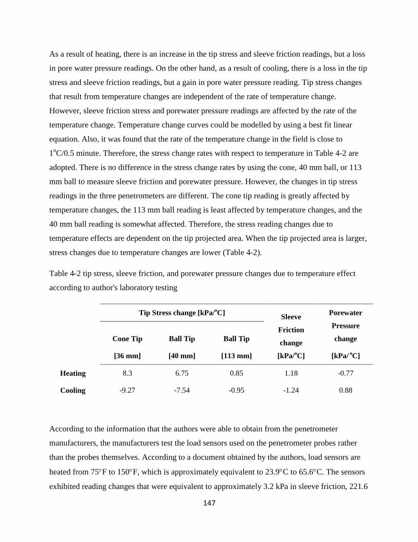
147
As a result of heating, there is an increase in the tip stress and sleeve friction readings, but a loss
in pore water pressure readings. On the other hand, as a result of cooling, there is a loss in the tip
stress and sleeve friction readings, but a gain in pore water pressure reading. Tip stress changes
that result from temperature changes are independent of the rate of temperature change.
However, sleeve friction stress and porewater pressure readings are affected by the rate of the
temperature change. Temperature change curves could be modelled by using a best fit linear
equation. Also, it was found that the rate of the temperature change in the field is close to
1oC/0.5 minute. Therefore, the stress change rates with respect to temperature in Table 4-2 are
adopted. There is no difference in the stress change rates by using the cone, 40 mm ball, or 113
mm ball to measure sleeve friction and porewater pressure. However, the changes in tip stress
readings in the three penetrometers are different. The cone tip reading is greatly affected by
temperature changes, the 113 mm ball reading is least affected by temperature changes, and the
40 mm ball reading is somewhat affected. Therefore, the stress reading changes due to
temperature effects are dependent on the tip projected area. When the tip projected area is larger,
stress changes due to temperature changes are lower (Table 4-2).
Table 4-2 tip stress, sleeve friction, and porewater pressure changes due to temperature effect
according to author's laboratory testing
Tip Stress change [kPa/oC]
Sleeve
Friction
change
[kPa/oC]
Porewater
Pressure
change
[kPa/ oC]
Cone Tip
[36 mm]
Ball Tip
[40 mm]
Ball Tip
[113 mm]
Heating 8.3 6.75 0.85 1.18 -0.77
Cooling -9.27 -7.54 -0.95 -1.24 0.88
According to the information that the authors were able to obtain from the penetrometer
manufacturers, the manufacturers test the load sensors used on the penetrometer probes rather
than the probes themselves. According to a document obtained by the authors, load sensors are
heated from 75F to 150F, which is approximately equivalent to 23.9C to 65.6C. The sensors
exhibited reading changes that were equivalent to approximately 3.2 kPa in sleeve friction, 221.6
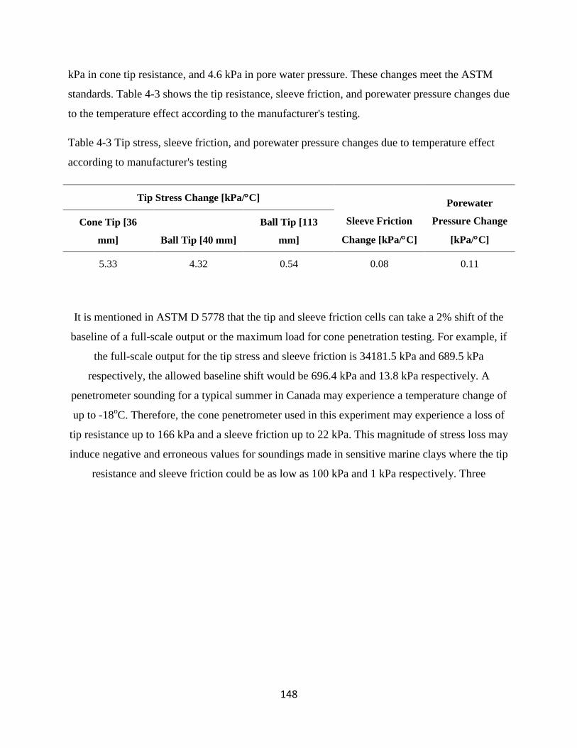
148
kPa in cone tip resistance, and 4.6 kPa in pore water pressure. These changes meet the ASTM
standards. Table 4-3 shows the tip resistance, sleeve friction, and porewater pressure changes due
to the temperature effect according to the manufacturer's testing.
Table 4-3 Tip stress, sleeve friction, and porewater pressure changes due to temperature effect
according to manufacturer's testing
Tip Stress Change [kPa/C]
Sleeve Friction
Change [kPa/C]
Porewater
Pressure Change
[kPa/C]
Cone Tip [36
mm] Ball Tip [40 mm]
Ball Tip [113
mm]
5.33 4.32 0.54 0.08 0.11
It is mentioned in ASTM D 5778 that the tip and sleeve friction cells can take a 2% shift of the
baseline of a full-scale output or the maximum load for cone penetration testing. For example, if
the full-scale output for the tip stress and sleeve friction is 34181.5 kPa and 689.5 kPa
respectively, the allowed baseline shift would be 696.4 kPa and 13.8 kPa respectively. A
penetrometer sounding for a typical summer in Canada may experience a temperature change of
up to -18oC. Therefore, the cone penetrometer used in this experiment may experience a loss of
tip resistance up to 166 kPa and a sleeve friction up to 22 kPa. This magnitude of stress loss may
induce negative and erroneous values for soundings made in sensitive marine clays where the tip
resistance and sleeve friction could be as low as 100 kPa and 1 kPa respectively. Three

149
temperature profiles with depth are shown in Figure 4-12 as an example.
Figure 4-12 temperature profile from three penetrometers tests
4.4 Results of the penetrometer tests and discussion
4.4.1 Soil Specific Cone Factors
4.4.1.1 Cone Penetrometer
Two CPTs were performed and the results are similar, see Figure 4-13. The tip resistance ranges
from approximately 100 to 800 kPa for a geodetic elevation of 61 to 78 m. Similarly, the sleeve
friction ranges from 1 to 19 kPa and porewater pressure from 100 to 650 kPa.
55
60
65
70
75
80
8 11 14 17 20 23 26 29
Geo
deti
c E
lev
ati
on
[m
]
Temperature [C]

150
Figure 4-13 cone penetration tests results with geodetic elevations for (a) tip resistance (b) sleeve
friction (c) porewater pressure, qt1 and qt2 are tip resistances for tests 1 and 2, fs1 and fs2 are
sleeve frictions for tests 1 and 2, u2(1) and u2(2) are porewater pressures for tests 1 and 2
Previous studies have shown that Nkt ranges between 8 and 16 for clays relative to triaxial and
direct shear tests (Aas et al. 1986; Lunne et al. 1997). The studies mentioned that this range is for
plasticity indexes between 3% and 50%. An increase in Nkt is also associated with a decreasing
plasticity index. Figure 4-14 shows that for this site, a decrease in the plasticity index is
associated with a general increase in Nkt at elevations of 66 and 75 m. This response is also
observed in the Nk and NΔu values at the same depths. It is also shown that Nkt can be between 11
and 18 (La Rochelle et al. 1988). Another study also mentioned that Nkt may vary between 8 and
29 relative to triaxial tests and also to the OCR (Rad and Lunne 1988). It was mentioned that Nkt
values may vary between 10 and 20 depending on the plasticity index, but this range may
increase to 10 and 30 in fissured and overconsolidated clays (Powell and Quarterman 1988). A
study was carried out on Danish till which provided Nkt values that ranged between 8.5 and 12
with an average of 10 (Luke 1995). At this site, Nkt values between 8.1 and 11.8 for only two
depth intervals were reported (DeJong et al. 2011). Similar values are obtained in this study.
However, temperature corrections are used. Temperature corrections have increased the Nkt
values from 2.4 to 8.1 to a similar range of that in previous studies which is 8.0 to 11.8 with an
55
60
65
70
75
80
0 1000 2000 3000
Geo
deti
c E
lev
ati
on
[m
] Tip Stress
[kPa]
qt1
qt2
0 10 20 30
Sleeve Friction [kPa]
fs1
fs2
0 400 800
Porewater Pressure
[kPa]
u2(1)
u2(2)

151
average of 9.4. Temperature corrections have also decreased the standard deviation of the Nkt
values from 1.5 to 1.1. Temperature corrections have also improved the values and decreased the
range and standard deviation for Nk and NΔu values for this site as shown in Table 4-4. For
normally consolidated clays, Nk values with reference to field vane tests vary between 11 and 19
with an average of 15 (Lunne and Kleven 1981). However, from this study, it was found that Nk
values, after temperature corrections, range between 6.0 and 11.3 with an average of 7.6 and
standard deviation of 1.2. It was found that NΔu values relative to field vane tests on three
Canadian clays range between 7 and 9 for an OCR that ranges from 1.2 to 50 (La Rochelle et al.
1988; Lunne et al. 1997). Another study used triaxial tests as reference and found that NΔu varies
between 6 and 8 (Karlsrud et al. 1996). From this study, after temperature corrections, the range
for NΔu values was found to be 5.5 to 10.4 with an average of 8.7 and standard deviation of 1.2.
The Nkt, Nk, and NΔu values are presented in Table 4-4.
Table 4-3 soil specific values for the cone tip
Without Temperature Correction With Temperature Correction
Nkt Nk NΔu Nkt Nk NΔu
Average 5.8 4.0 9.1 9.4 7.6 8.7
Range 2.4-8.1 0.5-7.8 5.8-10.7 8.0-11.8 6.0-11.3 5.5-10.4
STDev 1.5 1.6 1.3 1.1 1.2 1.2

152
Figure 4-14 cone soil specific factors and plasticity index with geodetic elevations, Nkt1 and
Nkt2 are cone soil specific factors from corrected tip resistance for cone tests 1 and 2, Nk1 and
Nk2 are cone soil specific factors from uncorrected tip resistance for cone tests 1 and 2, NΔu1
and NΔu2 are cone soil specific factors from excess porewater pressure for cone tests 1 and 2
Lunne et al. (1997) suggested that there is a correlation between Nkt and the pore pressure ratio
(Bq), which is the ratio of the excess porewater pressure to the difference between the corrected
tip resistance and the total overburden pressure. Their study suggested a range of 6 to 15 for Nkt,
which increases with a decreasing OCR. For this site, Nkt also seems to decrease when the pore
pressure ratio is increased and OCR is decreased, but with a range of 8.0 to 11.8 as shown in
Figure 4-15(a). Marsland and Powell (1988) and Powell and Quarterman (1988) proposed that
there is a correlation between the Nk value and the index of plasticity. Their study shows an
increase in Nk with an increase in the plasticity index. For this study, there is also a general
increase in Nk within a range of 6.0 to 11.3 with an increase in the plasticity index as shown in
Figure 4-15(b). Furthermore, the Nk values have a slightly higher scatter level with a high
plasticity index. Lunne and Lacasse (1985) found a correlation between NΔu and Bq for North
Sea clays that ranges from 4 to 10 with reference to triaxial tests. This study has also found that
60
65
70
75
80
6.0 9.0 12.0
Geo
deti
c E
lev
ati
on
[m
]
Nkt
Nkt1
Nkt2
4.0 8.0 12.0
Nk
Nk1
Nk2
10 30
Plasticity Index [%]

153
there is an increase in NΔu with increasing Bq, but for a range of 5.5 to 10.4 and reduced scatter
towards higher values of Bq as shown in Figure 4-15(c).
Figure 4-15 (a) cone soil specific factor Nkt from corrected tip resistance with porewater
pressure ratio (b) cone soil specific factor Nk from uncorrected tip resistance with plasticity
index(c) cone soil specific factor Nu from excess porewater pressure with porewater pressure
ratio
0
5
10
15
20
0.4 0.9 1.4
Nkt
Pore Pressure Ratio [Bq]
0
4
8
12
16
20
10 15 20 25 30
Nk
Plasticity Index [%]
0
5
10
15
20
0.4 0.6 0.8 1 1.2 1.4
Nu
Pore Pressure Ratio [Bq]

154
4.4.1.2 Ball Penetrometers
Two tests were carried out by using a ball penetrometer with a 40 mm ball and one was carried
out with a 113 mm ball (Figure 4-16). The tip resistance from the two 40 mm balls was
approximately the same. The tip resistance when the 40 mm ball was used ranged between 100
and 600 kPa from 61 to 88 m in terms of the geodetic elevation. The tip resistance when the 113
mm ball was used ranged between 0 and 450 kPa from 61 to 99 m in terms of the geodetic
elevation.
Figure 4-16 Net tip resistance with geodetic elevations for (a) 40 mm ball tip (b) 113 mm ball
tip, qb1 and qb2 are net tip resistances for 40 mm tip tests 1 and 2, qb(113mm) is net tip
resistance for 113mm ball tip test
Previous studies have proposed Nsu values for the penetrometer with a 113 mm ball from five
different sites (Yafrate and DeLong 2006; Yafrate et al. 2007; DeJong et al. 2009 and 2011). For
varved, medium stiff and lightly overconsolidated clays, a range from 9.6 to 11.0 was proposed
by DeGroot and Lutenegger (2003). For high plasticity, low overconsolidated, and soft to
medium stiff clayey silts, a range from 13.6 to 15.9 was proposed by Chung (2005). For highly
plastic and uniform marine clays with low OCR, Nsu values in the range of 11.4 to 12.5 were
obtained by Lunne et al. (2003). For Canadian sensitive marine clays, Louiseville in Quebec and
55
60
65
70
75
80
0 600 1200
Geo
deti
c E
lev
ati
on
[m
]
Net Tip Resistance [kPa]
qb1
qb2
0 600 1200
Net Tip Resistance [kPa]
qb(113 mm)

155
Gloucester in Ontario were considered. Louiseville has medium stiff homogeneous clay with
high plasticity and sensitivity. Nsu values proposed for Louiseville were 8.3 to 8.7. Gloucester,
on the other hand, has soft to medium stiff sensitive clay with three different layers. It was also
mentioned that the undrained shear strength ranges between 10 and 57 kPa and the sensitivity is
between 20 and 100. The proposed Nsu values were in the range of 5.8 to 6.0 for two depths.
However, from this study, it was found that the undrained shear strength ranges between 13 and
63 kPa and the sensitivity ranges between 0.5 and 26. The Nsu values from this study range
between 5.4 and 6.9 with an average of 6.2 and a standard deviation of 0.5; see Table 4-6 and
Figure 4-17(a). It is worth mentioning that temperature corrections do not seem to affect the
penetrometer with a 113 mm ball as much as that with a conventional cone due to the increased
projected area. The difference in Nsu before and after temperature correction is 0.3 and there is
no effect on the standard deviation (Table 4-6).
For the Canadian Geotechnical Research Site No. 1, an average value for Nsu-40 for the
penetrometer with a 40 mm ball is proposed. It was found that Nsu-40 ranges between 7.5 and 11.4
with an average of 8.5 and a standard deviation of 1.1 as indicated in Table 4-5. It can be noticed
that the penetrometer with a 40 mm ball is less affected by temperature correction than the
conventional cone penetrometer as a result of the increase in the tip projected area. The
difference between the corrected and uncorrected average values of Nsu-40 is 2.2 and there is no
difference in standard deviation. On the other hand, the difference between the average corrected
and uncorrected values of Nkt is 3.6 and the difference in the standard deviation is 0.4.
In order to meet the full-flow conditions, the tip projected area has to be ten times the projected
area of the push rods (Randolph 2004; Randolph and Anderson 2006; Boylan and Long 2007;
Yafrate et al. 2009; DeJong et al. 2010). Therefore, when reducing the tip projected area, the
push rods should also be reduced in size (Kelleher and Randolph 2005; Peuchen et al. 2005;
DeJong et al. 2010). Therefore, a penetrometer tip that is a 40 mm ball does not constitute a full-
flow penetrometer. A penetrometer tip that is a 40 mm ball was adopted for this study for ease of
field implementation. As part of the field practice, the top few feet from the surface were augered
in order to ensure that the penetrometer was pushed in a vertical direction as much as possible
into the ground and also to avoid possible damages to the penetrometer due to the presence of
surface rocks or boulders. Therefore, it is easier to use the penetrometer with a 40 mm ball and

156
augers than that with a 113 mm ball or T-bar. As the ratio of the tip projected area to push rods
decreases, the tip resistance increases up to a ratio of 1:1 where there is full displacement as in
the case of a cone tip. However, it has been mentioned that there is no significant increase or less
than 10% increase between a ratio of 10:1 and 5:1 (Chung and Randolph 2004; Weemees et al.
2006; Yafrate et al. 2007; DeJong et al. 2010). From this study, the tip resistance of the
penetrometer with a 40 mm and a 113 mm ball is approximately 44% and 54% respectively less
than that recorded with the cone tip. Therefore, the difference between the 10:1 ratio for the
penetrometer with the 113 mm ball and 1.26:1 for the penetrometer with the 40 mm ball is
approximately 10%. A point to emphasize here is that by using a penetrometer that has a ball for
the tip with a slightly larger diameter instead of that with a cone tip (40 mm as opposed to 36
mm), there is approximately a 44% decrease in the tip resistance.
Table 4-4 soil specific values for the 40 mm ball tip
Without Temperature Correction With Temperature Correction
Nsu-40 Nsu-40
Average 6.3 8.5
Range 4.6-9.1 7.5-11.4
STDev 1.1 1.1
Table 4-5 soil specific values for the 113 mm ball tip
Without Temperature Correction With Temperature Correction
Nsu Nsu
Average 5.9 6.2
Range 5.1-6.5 5.4-6.9
STDev 0.5 0.5

157
Figure 4-17 (a) ball soil specific factor Nsu-113-ball for 113 mm ball tip with geodetic elevation
(b) ball soil specific factor for 40 mm ball tip with geodetic elevation, Nsu1 and Nsu2 are ball
soil specific factors for 40 mm ball tests 1 and 2
4.4.2 Sensitivity Estimation
An undrained shear strength profile was obtained from the Nilcon vanes (Figure 4-18). The
undrained shear strength starts under a stress of 50 kPa at a geodetic elevation of 79 m, and then
drops to 13.4 kPa at a geodetic elevation of 78 m. Then, the undrained shear strength generally
increases up to 63 kPa at a geodetic elevation of 60 m. The remolded shear strength generally
follows the same pattern. The range of the sensitivity has a constant pattern of increase with
depth, which is between 1.9 and 8.0 with an outlier of 23.5 at a geodetic elevation of 78 m. It is
worth mentioning that the undrained shear strength ranges between 13 and 63 kPa which is
similar to the values mentioned by Bozozuk and Law (1976).
60
65
70
75
80
4.0 6.0 8.0
Geo
deti
c E
lev
ati
on
[m
]
Nsu-113-ball
6.0 9.0 12.0
Nsu-40-ball
Nsu1 Nsu2

158
Figure 4-18 (a) undrained shear strength with geodetic elevations from field vane tests (b)
sensitivity with geodetic elevations from field vane tests, Su is the initial undrained shear
strength, Sur is the remolded undrained shear strength
As mentioned earlier, remolded shear strength is recognized to be approximately equal to the
sleeve friction (Lunne et al. 1997). Therefore, sensitivity can be estimated by using the ratio of
the undrained shear strength that was estimated by using the tip resistance (qc) and the sleeve
friction. Sensitivity measured by field vane tests and sensitivity parameters from CPT with
respect to geodetic elevation is shown in Figure 4-19(a). There is a relatively good agreement
between the values obtained by the field vane tests and the estimated values especially in layers
with low sensitivity. The measurements of sensitivity from the field vane tests are plotted against
the estimations of sensitivity in Figure 4-19(b). There is good agreement between the values
from the field vane tests and the estimated values up to a sensitivity of around 8. Following this
value, there is considerably more scatter most likely due to that the method used for the
estimation of sensitivity which is not ideal for sensitive marine clays in Ottawa. To verify the
scattering observed in the estimation of sensitivity, the tip resistance is plotted against sleeve
friction in figure 4-19(c). There is good agreement, as indicated by a straight line, between the
tip resistance and sleeve friction up to a value of about 650 kPa for the former and 13 kPa for the
latter. Beyond 650 kPa and 13 kPa, the level of scattering considerably increases.
55
60
65
70
75
80
0 20 40 60
Geo
deti
c E
lev
ati
on
[m
] Shear Strength
[kPa]
Su(FVT)
Sur(FVT)
0.0 10.0 20.0 30.0
Sensitivity (FVT)

159
Figure 4-19 (a) sensitivity from cone penetration tests 1 and 2 St(CPT-1) and St(CPT-2) and
from field vane tests St(FVT) with geodetic elevations (b) sensitivity from cone penetration test
CPT with sensitivity from field vane tests FVT (c) sleeve friction with tip resistances from cone
penetration tests
58
63
68
73
78
0 5 10 15 20 25
Geo
deti
c E
lev
ati
on
[m
]
Sensitivity
St(CPT-1)
St(CPT-2)
St(FVT)
0
5
10
15
20
25
0 5 10 15 20 25
Sen
sit
ivit
y [
FV
T]
Sensitivity [CPT]
St(CPT-1)
St(CPT-2)
0
500
1000
1500
2000
2500
3000
0 10 20 30
Tip
Str
ess [
kP
a]
Sleeve Friction [kPa]

160
According to Schmertmann (1978), sensitivity can be estimated by using the ratio of Ns and the
friction ratio (Rf) in a percentage (Lunne et al. 1997). He suggested an Ns value of 15. Other
studies have suggested an Ns value of 6 with reference to vane tests (Robertson and Campanella
1988). Rad and Lunne (1986) found that Ns range between 5 and 10 with an average of 7.5.
Lunne et al. (1997) suggested an average value of 7.5 or a range of 6 to 9. However, they
claimed that there is no unique value for Ns as it depends on the mineralogy and OCR. They also
suggested the calibrating of Ns with local experience, especially with sensitive clays when the
sleeve friction readings are low. From this research, the average value of Ns was found to be 7.0,
which is similar to the recommended 7.5. However, a relatively large range was encountered,
from 2.3 to 15.9, with a standard deviation of 3.0. figure 4-20(a) shows the variation of Ns with
geodetic depth for two CPT soundings. It can be noticed that there is a reverse relationship
between the plasticity and the sensitivity represented by Ns as shown in a comparison, see Figure
4-20(a) and Figure 4-20(b).
It is worth mentioning that the sensitivity of this site ranges between 2 and 23, unlike the values
reported by Yafrate and DeLong (2006) of up to a hundred.

161
Figure 4-20 (a) sensitivity factor Ns from cone penetration tests 1 and 2 CPT-1 and CPT-2 (b)
plasticity index with geodetic elevations for the purpose of comparison
4.4.3 Soil Geotechnical profile
Figure 4-21 shows the soil type by using CPT sounding per Jefferies and Davies (1991) and soil
classification by using the Cassagrande plasticity chart (CPC). It can be seen that soil that
comprises high plasticity inorganic clay per the CPC is recognized as clay by the CPT. Low to
medium plasticity inorganic clay or silty clay is recognized as organic soil. There is a difference
in the geodetic elevation of the layers probably due to the interlayers and stratification. The CPT
does not appear to recognize the medium to high plasticity organic clay to silty clay.
60
65
70
75
80
0.0 10.0 20.0 30.0
Ge
od
eti
c El
eva
tio
n [
m]
Ns
CPT-1
CPT-2
10 20 30
Plasticity Index [%]

162
Figure 4-21 (a) soil type classification according to Jefferies and Davies (1991) for cone
penetration test 1 with geodetic elevations (b) soil type classification according to Jefferies and
Davies (1991) for cone penetration test 2 with geodetic elevations (c) soil type according to
Cassagrande's Plasticity Chart CPC from plasticity results with geodetic elevations, horizontal
axis is the soil class number or number representing the soil name
According to the fines content (silt and clay portion) suggested by Lunne et al. (1997), Suzuki et
al. (1995), and Robertson (1990), fines content from hydrometer testing in the laboratory and
cone penetration testing are plotted with geodetic elevation as in Figure 4-22. There is an
underestimation in the fines content. The actual fines content is close to 100% while the CPT
provides an average of about 60%.
58
60
62
64
66
68
70
72
74
76
78
80
0 1 2 3 4
Geo
deti
c E
lev
ati
on
[m
] CPT-1
0 1 2 3 4
CPT-2
5 6 7 8 9
CPC
1-Clay
2-Organic Soil
3-Clayey Silt to Silty Clay
6-low to medium plasticity inorganic clay or silty clay
7-high plasticity inorganic clay
8-medium to high plasticity organic clay or silt

163
Figure 4-22 fines content according to the method suggested by Lunne et. al. (1997) from cone
penetration tests 1 and 2 FC (CPT-1) and FC (CPT-2) and from laboratory testing FC with
geodetic elevations
According to the plasticity limits and moisture contents recorded with geodetic elevation, all of
the soil profiles have exceeded the liquid limits except at an elevation of 62 m where they are
close to the liquid limit. This explains the small tip resistance and sleeve friction recorded in the
penetrometer pushes. The plastic limits, liquid limits, and plasticity index are all affected by the
varved deposition of sensitive marine clays. As the silt content increases, the plastic limits, liquid
limits, and plasticity index decrease, such as at elevations of 60.5 and 66.5 m, see Figure 4-6.
4.4.4 Consolidation History
Lunne et al. (1997) mentioned that if Qt is within 2.5 to 5, then the soil is normally consolidated.
However, if Qt is greater than this range, then the soil is overconsolidated. From Figure 4-23(a),
it can be seen that the soil is lightly overconsolidated at about an elevation of 76 m and above,
while Qt exceeds 5 only when the elevation is greater than 78 m, as shown in Figure 4-23(b).
This is probably a result of the interlayers and stratification. An average k value of 0.3 was
proposed by Robertson (2000) with a range of 0.2 to 0.5, and higher values are recommended for
aged and heavily overconsolidated soils. From this research, an average value of 0.44 was
60
65
70
75
80
20 40 60 80 100 120
Geo
deti
c E
lev
ati
on
[m
]
Fines Content [%]
FC
FC(CPT-1)
FC(CPT-2)

164
obtained with a range of 0.21 to 0.56 with outliers of 1.14 and 1.4 for CPT 2 at geodetic
elevations of 74.3 and 76.6 m respectively, and a standard deviation of 0.34, see Figure 4-23(c).
Figure 4-23 (a) normalized tip resistance from cone penetration tests 1 and 2 Qt(CPT-1) and
Qt(CPT-2) with geodetic elevations (b) overconsolidation ratio from laboratory testing with
geodetic elevation for the purpose of comparison (c) k factor for consolidation history from cone
penetration tests 1 and 2 k(CPT-1) and k(CPT-2) with geodetic elevations
For sites with available data, the correlation of OCR with other parameters is suggested, such as
Qt and Bq, in order to better estimate the OCR and preconsolidation ratio. However, from this
research, the correlation of OCR with Qt and Bq is scattered and does not follow a clear pattern
as shown in Figure 4-24. The reason is that these correlations do not apply well to sensitive
marine clays in Ottawa.
58
60
62
64
66
68
70
72
74
76
78
80
0 2.5 5 7.5 10 12.5 15
Ge
od
eti
c E
leva
tio
n [
m]
Normalized Tip Resistance
Qt(CPT-1)
Qt(CPT-2)
0.0 1.0 2.0
Overconsolidation Ratio
0.00 0.75
k
k(CPT-1)
k(CPT-2)

165
Figure 4-24 overconsolidation ratio from laboratory testing with (a) normalized tip resistance
from cone penetration tests 1 and 2 Qt(CPT-1) and Qt(CPT-2) (b) porewater pressure ratio from
cone penetration tests 1 and 2 Bq(CPT-1) and Bq(CPT-2)
Chen and Mayne (1996) studied the relationships between CPTs and the stress history of
different types of soils from around the world including Canadian soil. They indicated that
correlations of preconsolidation pressure and stress difference such as qt-σov, Δum, and qt-um
render better estimations that those that incorporated Bq. They also indicated that the
incorporating of Ip may increase accuracy in estimation.
4.5 Summary and conclusions
Sensitive marine clay deposits in Ottawa have been characterized by using penetrometer tests.
The Canadian Geotechnical Research Site No. 1 has been the target of researchers as a
representative site of sensitive marine clays in Ottawa. Correlations between penetrometer tests
and soil engineering characteristics have been developed in the literature. However, it is
recommended that these correlations be verified and modified in accordance with local and site
specific experiences. Temperature effects on penetrometer readings have also been verified.
Samples from cone penetration, ball penetrometer and vane tests, as well as undisturbed samples,
2
3
4
5
6
0.4 0.8 1.2 1.6
No
rmalized
Tip
Resis
tan
ce
OCR
Qt(CPT-1)
Qt(CPT-2)
0.4
0.6
0.8
1
1.2
1.4
0.4 0.8 1.2 1.6 P
ore
wate
r P
ressu
re R
ati
o
OCR
Bq(CPT-1)
Bq(CPT-2)

166
have been collected from the site. A penetrometer with a tip that is a 40 mm ball is pushed into
sensitive marine clays for the first time to verify the suitability of this type of tip for the soil. It is
used for the ease of implementation in the field. It is found that there is a decrease in the tip
stress of approximately 44% when the tip is a ball that is slightly larger than a cone tip.
Typically, the tip stress drops as the tip projected area increases. Laboratory tests are performed
on the undisturbed samples as reference for the field data.
In terms of the cone equipment used in this study, it is found that a temperature change of 18C
may cause a gain or loss of 166 kPa and 22 kPa in tip resistance and sleeve friction readings
respectively. This effect may result in negative and erroneous readings from penetrometers. A
temperature correction factor is established for the specific penetrometers used in this experiment
and applied to each tip, sleeve, and pore pressure reading.
Empirical correlations between CPTs and soil engineering properties have been verified for
sensitive clays in Ottawa. The correlation of the undrained shear strength with the CPT
parameters, Nkt, Nk, NΔu, have average values of 9.4, 7.6, and 8.7 respectively. The correlation
factor, NSu-40, of the undrained shear strength based on tests carried out by a penetrometer with a
40 mm ball is 8.5. The correlation factor, NSu, of the undrained shear strength based on tests
carried out by a penetrometer with a 113 mm ball is 6.2. It is found that NSu has a smaller range
and standard deviation than those of the CPTs and tests carried out by the penetrometer with a 40
mm ball. It is also found that the penetrometer with a 113 mm ball is the least affected by
temperature change. The sensitivity has a reduced value of scattering up to 8 where then, the
scattering considerably increases. The sensitivity correlation factor, Ns, has an average value that
is equal to 7.0. The consolidation history factor, k, has an average value of 0.44. It is
recommended that the correlation of the consolidation history be modified with normalized tip
resistance and porewater pressure ratio. However, no clear relation is found with the OCR. Grain
size profile and soil types from the CPC are compared with the method used in Jefferies and
Davies (1991) to determine soil behaviour. It is found that CPC can correctly detect layers with
coarser grain sizes, but not organic layers. More specific zones need to be determined for
sensitive marine clays in Ottawa. The fines content is also underestimated.

167
Acknowledgement
This research is in fulfillment of IPS NSERC that is a joint scholarship program for Mr. Athir
Nader between the University of Ottawa represented by Prof. Mamadou Fall and Stantec
Consulting Limited represented by Mr. Raymond Hache. Field work for this research is
provided by Marathon Drilling Cooperation Limited.
4.6 References
Aas, G., Lacasse, S., Lunne, T., & Hoeg, K. (1986). Use of in situ tests for foundation design on
clay. Proceedings of the ASCE Specialty conference in situ's 86: use of in situ tests in
geotechnical engineering 1-30. ASCE, Blacksburg.
Aber, J. S. (2005, 2). Glacial Geology of the Kansas City Vicinty. U.S. Forest Service. Retrieved
7 8, 2013, from http://www.geospectra.net/lewis_cl/geology/glacial.htm
Almeida, M. S. S., Danziger, F. A. B, Lunne, T. (1996). Use of piezocone test to predict the axial
capacity of driven and jacked piles in clay. Canadian Geotechnical journal 33(1):33-41.
Andrews, J. T. (1972). The National Atlas of Canada. Mines and Resources, Canada Department
of Energy,.
Andrews, J. T. (1986). The pattern and interpretation of restrained, post-glacial and residual
rebound in the area of Hudson Bay. Geological Survey of Canada Paper 49-62.
Andrews, J. T., Peltier, W. R. (1976). Collapse of the Hudson Bay ice centre and glacio-isostatic
rebound. Geology 4:73-75.
ASTM D 4318 – 05 (April 2005). Standard Test Methods forLiquid limit, Plastic limit, and
Plasticity Index of soils.
Ballivy, G., Loiselle, A. A., Pouliot, G. (1975). Quelques caractkristiques gkotechniques des
d'pBts d'argile de la baie James: les coulCes d'argile de Fort Rupert, Quebec. Canadian
Geotechnical Journal 12:498-509.

168
Ballivy, G., Pouliot, G., Loiselle, A. (1971). Quelques caracteristiques geologique et
mineralogiques des depots d'argile du nord-ouest du Quebec. Canadian Journal of Earth
Sciences 8:1525-1541.
Battaglio, M., Jamiolkowsi, M., Lancellotta, R., & Maniscalco, R. (1981). Piezometer probe test
in cohesive deposits. Proceedings of the Session ASCE National Convention 264-302. St. Louis.
Bentley, S. P., Smalley, I. J. (1979). Mineralogy of a leda/champlain clay from gloucester.
Engineering Geology 14:209-217.
Bentley, S. P., Smalley, I. J. (1978). Mineralogy of sensitive clays from Quebec. Canadian
Mineralogist 16:103-112.
Berry, R. W. (1988). Mineralogyg,r ain.sizde istributioann dg eotechnicable havior. The
Canndian Mineralogist 36:1625-1636.
Boissonneau, A. (1966). Glacial history of northeastern Ontario: I. The Cochrane-Hearst area.
Canadian Journal of Earth Sciences 3:559-578.
Boylan, N., & Long, M. (2007). Characterization of peat using full flow penetrometers. Soft Soil
Engineering.
Boylan, N., Long, M., & Mathijssen, F. (2011). In situ strength characterization of peat and
organic soil using full-flow penetrometers. Canadian Geotechnical Journal 48:1085-1099.
Briaud, J.-L. (2007). Spread foorings in sand: Load-settlement curve approach. Journal of
Geotechnical and Geoenvironmental Engineering 133(8):905-920.
Brydon, J. E., Patry, L. M. (1961). Mineralogy of Champalin Sea sediments and a Rideau clay
soil profile. Canadian Journal of soil science 41:169-181.
Campanella, R., Robertson, P., Gillespie, D., & Greig, J. (1985). Recent developments in in-situ
testing of soils. Proceedings of the 11th International Conference on Soil Mechanics and
Foundation Engineering 849-54. Balkema Pub, San Francisco.
Chen, P., & Mayne, P. (1996). Statistical relationships between piezocone measurements and
stress history of clays. Canadian Geotechnical Journal 33:488-498.

169
Chung, S. (2005). Characterization of soft soils for deep water developments. Nedlands,
Australia: Department of civil and resources engineering, the University of Weatern Australia.
Chung, S., & Randolph, M. (2004). Penetration resistance in soft clay for different shaped
penetrometers. ISC-2 on Geotechnical and Geophysical Site Characterization 671-677. :
Millpress , Porto.
Crawford, C. (1968). Quick clays of eastern Canada. Engineering Geology 2(4):239-265.
Crawford, C., & Eden, W. (1965). A comparison of laboratory results with in situ properties of
Leda clay. Proc. Ontern. Conf. Soil Mech. Found. Eng., 6th 1:31-35. Montreal.
Cronin, T. M. (1977). Late-Wisconsin marine environments of the Champlain Valley 7:238-253.
Quaternary Research, New York, Quebec..
DeGroot, D., & Lutenegger, A. (2003). Geology and engineering properties of connecticut vally
varved clay. In T. Tan, K. Phoon, D. Hight, & S. Lerouell, Characterization and engineering
properties of natural soils 695-724. Rotterdam.
DeJong, J. T., Yafrate, N. J., & DeGroot, D. J. (2011). Evaluation of undrained shear strength
using full-flow penetrometers. Journal of geotechncial and Geological Engineering 14-26.
DeJong, J., DeGroot, D., & Randolph, M. (2009). Evaluation of shear strength and sensitivity of
soft clay using full-flow penetrometers. Journal of Geotechnical and Geological Engineering
1179-1189.
DeJong, J., Yafrate, N., & Randolph, M. (2008). Use of pore pressure measurements in a ball
full flow penetrometer. Geotechnical and Geophysical Site Characterization 1269-1275. Taipei:
Taylor and Francis.
DeJong, J., Yafrate, N., DeGroot, D., Low, H. E., & Randolph, M. (2010). Recommended
practice for full-flow penetrometer testing and analysis. Geotechnical Testing Journal 33
Demers, D. L. (2002). Evaluation of preconsolidation pressure and the overconsolidation ratio
from piezocone tests of clay deposits in Quebec. Canadian Geotechnical Journal 39(1):174-192.

170
Dreimanis, A. (1976). Tills: Their origin and properties. Royal society of Canada Special
Publication 12:11-49.
Dreimanis, A. (1977). Correlation of Wisconsin glacial events between the eastern Great Lakes
and the St. Lawrence Lowlands. Gkographie, Physique et Quaternaire 37-51.
Dreimanis, A. (1977). Late Wisconsin glacial retreat in the Great Lakes region, North America.
Annals of the New York Academy of Sciences 288:70-89.
Elson, J. A. (1967). Geology of glacial Lake Agassiz. University of Manitoba Press 36-95.
Fall, M. (2011). Geotechnical Hazards Lectures Notes- The University of Ottawa.
Fanning, D.S., Jackson, M.L. (1966). Clay mineral weathering in southern Wisconsin soils
developed in loess and in shale-derived till. Proceedings, 13th Conference 175-191.
Gadd, N. (1962). Surficial geology of Ottawa map-area Ontario and Quebec. Geol. Sutv. Can.,
Paper 62(16):4.
Gadd, N. R. (1975). Geology of Leda clay. Geo Abstracts Ltd 137-151.
Gillott, J. E. (1971). Mineralogy of Leda clay. Canadian Mineralogist 10:797-811.
Group, N. P. (1971). Nature of Quickclays. Nature 231.
Hendershot, W. H., Carson, M. A. (1978). Changes in the plasticity of a sample of Champlain
clay after selective chemical dissolution to remove amorphous material. Canadian Geotechnical
Journal 15:609-616.
Hillaire-Marcel, M. C. (Published these de Doctorat d'Etat ks Sciences Naturelles, Universitk
Pierre et Marie Curie, Paris). 1979. Les nlers post-glaciaires du Quebec: quelques aspects
Houston, W. N., Mitchell, J. K. (1969). Property interrelationships in sensitive clays. ASCE
Journal of the Soil Mechanics and Foundation Division 95:1037-1062.
Jamiolkowski, M., Ladd, C., Germaine, J., & Lancellotta, R. (1985). New developments in field
and laboratory testing of soils. 11th International Conference on Soil Mechanics and
Foundation Engineering 57-153. San Francisco.
171
Jefferies, M., & Davies, M. (1991). Soil classification by the cone penetration test. Canadian
Geotechnical Journal 28(1):173-6.
Johnston, W. (1917). Pleistocene and recent deposits in the vicinity of Ottawa, with a description
of the soils. Geo. Surv. Can., Mem. 101:69.
Jones, G. A., Van Zyl, D. J. A. (1981). The piezometer probe: a useful invertigation tool. 10th
internation conference of soil mechanics and foundation engineering 3:489-495.
Karlsrud, K., Lunne, T., & Brattlien, K. (1996). Improved CPTU correlations based on block
samples. Nordic Geotechnical Conference 195-201. Reykjavik.
Karrow, P. (1961). The Champlain Sea and its sediments. R. F. Legget (Editor), Soils in Canada.
Roy. Soc. Can. Spec. Publ. 3:97-108.
Kelleher, P., & Randolph, M. (2005). Seabed geotechnical characterisation with a ball
penetrometer deployed from the portable remotely operated drill. Frontier in Geotechnics, Perth
365-371.
Kenney, T. (1964). Sea-level movements and the geologic histories of the post-Glacial marine
soils at Boston, Nicolet, Ottawa and Oslo. Geotechnique 14:203-230.
Kenney, T. (1976). Formation and geotechnical characteristics of glacial-lake varved soils.
Norwegian Geotechnical Institute Publication 15-39.
Konrad, K., & Law, J. (1987). Undrained shear strength from piezocone tests. Canadian
Geotechnical Journal 24:392-405.
Kulhawy, F. H., Mayne, P. W. (1993). Drilled shaft side resistance in clay soil to rock. design
and performance of deep foundation 172-183.
Kulhawy, F., & Mayne, P. (1990). Manual on estimating soil properties for foundation design.
Electrical Power Research Institute.
La Rochelle, P., Lefebvre, G. (1971a). Sampling disturbance in Champlain clays. American
society for testing and materials 483:143-163.

172
La Rochelle, P., Zebdi, P., Leroueil, S., Tevenas, F., & Virely, D. (1988). Piezocone tests in
sensitive clays in eastern Canada. Preceedings of the International Symposium on Penetration
Testing 831-41. Balkema Pub , Rotterdam.
Lee, K. L. (1979). Cyclic strength of a sensitive clay of eastern Canada. Canadian Geotechnical
Journal 16:163-176.
Leroueil, S. (1999). Geotechnical characteristics of eastern Canada clays. Characteristics of
Soft Marine Clays, ISBN 90 5809 104X.
Leroueil, S. (1999). Geotechnical characteristics of eastern Canada clays. Characteristics of
Soft Marine Clays, ISBN 90 5809 104X.
Letoueil, S., Tavenas, F., Le Bihan, J. P. (1983a). Proprietes caracteristiques des argiles de l'est
du Canada. Canadian Geotechnical journal 20(4):681-705.
Lo, K. Y., Bozozuk, M., & Law, K. T. (1976). Settlement analysis of the Gloucester test fill.
Canadian Geotechnical Journal 13(4):341-354.
Lo, K. Y., Ho, K. S. (1991). The effects of electroosmotic field treatment on the soil properties of
a soft sensitive clay. Canadian Geotechnical Journal 28:763-770.
Locat, E. D. (1996). O n the developmenot f microstructurein. In Genesis and Properties of
Collapsible 93-128.
Low, H., Lunne, K., Andersen, M., Li, X., & Randolph, M. (2010). Estimation of intact undrained
shear strength from penetration tests in soft clays. Geotechnique 11:843-859.
Luke, K. (1995). The use of cu from Danish triaxial tests to calculate the cone factor.
Preceedings of the International Symposium on Cone Penetration Testing 209-14. Linkoping,
Sweden: Swedish Geotechnical Society.
Lunne, T., & Kleven, A. (1981). Role of CPT in north sea foundation engineering. Session at the
ASCE National Convention: Cone Penetration testing and Materials 76-107. ASCE, St. Louis.

173
Lunne, T., & Lacasse, S. (1985). Use of in situ tests in North Sea soil investigations. Proceedings
of the Symposium: From Theory to Practice in Deep Foundations 169. Norwegian geotechnical
Institute, Porto Allegre, Brazil.
Lunne, T., Long, M., & Forsber, C. (2003). Characterization and engineering properties of
Onsoy clay. In T. Tan, K. Phoon, D. Hight, & S. Lerouell, Characterization and engineering
properties of natural soils 395-427. The Netherlands: eds, Rotterdam.
Lunne, T., Robertson, P. K., Powell, J. J. M. (1997). Cone Penetration Testing in Geotechnical
Practise. Blackie Academic , New York.
Lunne, T., Robertson, P., & Powell, J. (1997). Cone Penetration Testing. Blackie Academic &
Professional.
Marsland, A., & Powell, J. (1988). Investigation of cone penetration tests in British clays carried
out by the Building Research Establishment 1962-1987. Preceedings of the Geotechnology
Conference: Penetration Testing in the UK 209-14. Thomas Telford, London.
Massarsch, K., & Broms, B. (1981). Pile driving in clay slopes. Proceedings of the 10th
International Conference on Soil Mechanics and Foundation Engineering 469-74. : Balkema
Pub, Stockholm.
May, R. (1977). Facies model for sedimentation in the glaciolacustrine environment. Boreas,
6:175-180.
Mayne, P. W. (2009). Engineering Design Using the Cone Penetration Test-Geotechnical
Application Guide. ConeTec.
Mayne, P. W., Kulhawy, F. H. (1982). Ko-OCR relationship in soils. Journal of Geotechnical
Engineering 106:851-872.
Mayne, P. W., Stewart, H. E. (1988). Pore pressure response of K-consolidated clays. Journal of
Geotechnical Engineering 114(11):1340-1346.
Morgenstren, N. (1967). Submarine slumping and the initiation of turbidity currents. University
of Illinois Press 189-220.

174
Nagaraj, T. S., Murthy, B. R. S., Vatsala, A., Joshi, R. C. (1990). Journal of Analysis of
compressibility of sensitive soils 116(1):105–118.
Nishimura, T., Hirabayashi, Y. Fredlund, D. G., Gan, J. K. M. (1999). Influence of stress history
on the strength parameters of an unsaturated statically compacted soil. Canadian Geotechnical
Journal 36:251-261.
Peck, R. B., Ireland, H. O., Fry, T. S. (1951). U illinois civ. Eng. Dep. soil Mech. series no.1.
Penner, E. (1965). A study of the sensitivity of Leda clay. Canadian Journal of Earth Sciences 2.
Penner, E. (1970). Frost heaving forces in Leda Clay1. Canadian Geotechnical Journal 7:8.
Peuchen, J., Adrichem, J., & Hefer, P. (2005). Practice notes on push-in penetrometers for
offshore geotechnical investigation. Proceedings of the International Symposium on Frontiers in
Offshore Geotechnics 973-979. Perth, Australia: Taylor & Francis, London.
Poulus, H. G., Davis, E. E. (1974). Elastic solutions for soil and rock mechanics. John Wiley and
sons Inc.213.
Powell, J., & Quarterman, R. (1988). The interpretation of cone penetration tests in clays with
particular reference to rate effects. Proceedings of the The International Symposium on
Penetration Testing 903-10. Balkema Pub, Rotterdam.
Push, R., Arnold, M. (1969). Engineering Geology 3:135.
Quigley R.M., T. (1976). Till geology, mineralogy and geotechnical behaviour, Sarnia, Ontario.
Royal Society of Canada Special Publication 12:336-345.
Quigley, R. M. (1980). Geology, mineralogy, and geochemistry of Canadian soft soils: a
geotechnical perspective. Canadian Geotechnical Journal 17:261-285.
Rad, N., & Lunne, T. (1986). Correlations between piezocone results and laboratory soil
properties. Norwegian Geotechnical Institute, Oslo.

175
Rad, N., & Lunne, T. (1988). Directed correlations between piezocone test results and undrained
shear strength of clay. Preceedings of the International Symposium on Penetration Testing 911-
17. Balkema Pub, Rotterdam.
Randolph, F., Hefer, P. A., Geise, J. M., & Watson, P. (1998). Improved seabed strength using
T-bar penetrometer. Proceedings of the International Conference on Offshore Site Investigation
and Foundation Behaviour (pp. 221-235). Society for Underwater Technology, London.
Randolph, M. (2004). Characterization of soft sediments for offshore applications. ISC-2 on
Geotechnical and Geophysical Site Characterization 209-232. Millpress, The Netherlands.
Randolph, M., & Anderson, K. (2006). Numerical analysis T-bar penetration in soft clay. Int. J.
Geomech. 6:411-152.
Randolph, M., & Wroth, C. (1979). An analytical solution for the consolidation around a driven
pile. Proceedings of the International Journal for Numerical and Analytical methods in
Geotechnics 217-29.
Randolph, M., Low, H., & Zhou, H. (2007). In situ testing for design of pipeline and anchoring
systems. Proceedings of the Sixth International Conference on Offshore Site Investigation and
Geotechnics 251-262. Society for Underwater Technology, London.
Robertson, P. (1990). Soil classification using the cone penetration test. Canadian Geotechnical
Journal 27(1):151-8.
Robertson, P. (2000). Cone Penetration Testing Geotechnical Application Guide. Cone Tec Inc.
& Gregg In Situ Inc.
Robertson, P. K. (1990). Soil classification using the cone penetration test. Canadian
Geotechnical Journal 27:151-158.
Robertson, P. K. (2004). Evaluating soil liquifaction and post-earthquake defor-mations using
the CPT Geotechnical and Geophysical Site Characteristics. Millpress, Rotterdam 1:233-249.
Robertson, P., & Campanella, R. (1983). Interpretation of cone penetration test. Canadian
Geotechnical Journal 20(4):734-45.

176
Robertson, P., & Campanella, R. (1988). Guidelines for geotechnical design using CPT and
CPTU. University of British Columbia, Department of Civil Engineering, Vancouver.
Robertson, P., Campanella, R., Gillespie, D., & Greig, J. (1986). Use of piezometer cone data.
Proceedings of the ASCE Specialty Conference In Situ '86: Use of In Situ tests in Geotechnical
Engineering 1263-80. ASCE, Blacksburg.
Robertson, P., Sully, J., & Woeller, D. (1990). Guidelines for interpretation of CPTU test data
for determination of consolidation and permeability parameters of soils. ConeTec Investigations
Ltd. for Energy, Mines and Resources Canada.
Roy, M., Blanchet, R., Tavenas, F., La Rochelle, P. (1981). Behaviour of a sensitive clay during
pile driving. Canadian Geotechnical Journal 18:67-85.
Saihi, F., Leroueil, S., La Rochelle, P., French, I. (2002) Behaviour of the stiff and sensitive
saint-jean-vianney clay in intact, destructed, and remoulded conditions. Canadian Geotechnical
Journal 39:1075–1087.
Schmertman, J. (1978). Guidelines for cone penetration test, performance and design.US
Federal Highway Administration, Washingto, DC
Senneset, K., Sandven, R., Lunne, T., Amundsen, T. (1988). Piezocone tests in silty soils.
Proc.ISOPT-Orlando 2:955-974.
Simon, G., Hache, R., Fred, J. G. (Dec 2010). Esprit Drive Overpass-Cumberland Transitway.
Stantec Consulting Ltd, Ottawa.
Simon, G., Hache, R., Fred, J. G. (Dec 2010). Portbello Boulevard Overpass-Cumberlan
Transitway Project. Stantec Consulting Ltd, Ottawa.
Smith, N. (1978). Sedimentation processes and patterns in a glacier-fed lake with low sediment
input. Canadian Geotechnical Journal 15:741-756.
Soderman, L. G., Quigley, R. M. (1965). Geotechnical properties of three Ontario clays.
Canadian Geotechnical Jounal 2:167-189.

177
Stewart, D., & Randolph, M. (2001). A new site investigation tool for the centrifuge. Proceedings
of the International Conference Modelling 531-538. Balkema, The Netherlands.
Suzuki, Y., Tokimatsu, K., & Kubota, Y. (1995). Correlation between CPT data and dynamic
properties of in situ frozen samples. Proceedings of the Third International Conference on
Recent Andances in Geotechnical Earthquake Engineering and Soil Dynamics 249-52.
University of Missouri Rolla, St. Louis.
Syvitski, J. (1980). Flocculation, agglomeration and zooplankton pelletization of suspended
sedinient in a fjord receiving glacial meltwater. In Fjord oceanography 616-625. NATO
Conference 4.
Syvitski, J. P. (1978). Sedimentological advances concerning the flocculation and zooplankton
pelletization of suspended sediment in Howe Sound, British Columbia: A fjord receiving glacial
meltwater.Ph.D. thesis, University of British Columbia, British Columbia, Vancouver, B.C.
Syvitski, J. P., Murray, J. W. (1980). Particle interaction in fjord suspended sediment. Marine
Geology. In Press.
Tavenas, F., Tremblay, M., Larouche, G., Leroueil, S. (1986). In situ measurement of
permeability in soft clays. ASCE Special Conf. 1034-1048.
Tevanas, F., Leroueil, S. (1987). State-of-the-art on laboratory and in-situ stress-strain-time
behaviour of soft clays. International Symposium on Geotechnical Engineering of soft soils 1-
146.
Torrance. (1988). Mineralogy, pore-water chemistry. In The late Quaternary Developmen
35:259-275.
Torrance, J. K. (1979). Post-depositional changes in the pore water chemistry of the sensitive
marine clays of the Ottawa area, eastern Canada. Canada Engineering Geology 14:135-147.
Walker, L. K., Raymond, G. P. (1966). The prediction of consolidation rates. Canadian
Geotechnical Journal 4:101-107

178
Walker, L. K., Raymond, G. P. (1969). Anisotropic consolidation of Leda clay. Canadian
Geotechnical Journal 6:271.
Watson, P., Newson, T., & Randolph, M. (1998). Strength profiling in soft offshore soils. In
Proceedings of the 1st International Conference on Site Characterisation (pp. 1389-1394).
Atlanta: Edited by Robertson, P.K., Mayne, A.A. Balkema, Rotterdam, the Netherlands .
Weemees, L., Howie, J., Woeller, D., & Sharp, J. (2006). Improved techniques for the in situ
determination of undrained shear strength of soft clays. Sea to Sky Geotechnique 89-95.
Vancouver, Canada.
Williams, G., & Gold, L. (1976). Ground temperatures. National Research Council Canada 180-
4.
Yafrate, N. J., & DeLong, J. T. (2006). Interpretation of sensitivity and remolded shear strength
with full flow penetrometers. Civil & Environmental Engineering, University of California, CA,
USA.
Yafrate, N., & DeJong, J. (2006). Interpretation of sensitivity and remolded undrained shear
strength with full flow penetrometers. Davis, CA, USA.
Yafrate, N., DeJong, J., & DeGroot, D. (2007). The influence of full-flow penetrometer area
ratio on undrained strength measurements. Proceedings of 6th International Conference on
Offshore Site Investigation and Geotechnics 461-468. Society for Underwater Technology,
London.
Yafrate, N., DeJong, J., DeGroot, D., & Randolph, M. (2009). Evaluation of remolded shear
strength and sensitivity of soft clay using full-flow penetrometers. J. Geotech. Geoenviron. Eng.
135:1179-1189.
Yong, R. N., Sethi, A. J., La Rochelle, P. (1979). significance of amorphous material relative to
sensitivity in some Champlain clays. Canadian Geotechnical Journal 16:511-520.
Yong, R. N., Silvestri, V. (1979). Anisotropic behaviour of a sensitive clay. Canadian
Geotechnical Journal 16:335-350.

179
Chapter 5 Conclusions and Recommendations
5.1 Summary
In this thesis, the engineering characteristics of sensitive marine clays in Ottawa have been
assessed. There has been an attempt to provide background and reference information for
geotechnical engineers who are working with these soils. The thesis has also provided
background about the origin, geological settings, sedimentation, and structure of sensitive marine
deposits. Two correlations in the Canadian Foundation Engineering Manual have been
examined. The first correlation is between SPTs and undrained shear strength. The second
correlation is between shear wave velocity and undrained shear strength, and site class. Values
have been compared in terms of the ratio of the secondary compression index to the compression
index proposed by previous researchers and this research. In general, this thesis has proposed
ranges of values for engineering characteristics based on fifteen sites and those by previous
researchers.
This thesis has studied the effect of temperature on cone penetration testing in sensitive marine
clays in Ottawa. Correlations between CPTs and the engineering characteristics of these clays are
examined. Furthermore, the values of the coefficient of consolidation from oedometer and pore
pressure dissipation testing have been examined by using CPTs. The work here has also
attempted to increase local experience on the use of ball penetrometers in these clays.
5.2 Conclusions and Future Research Recommendations
The following conclusions and recommendations are made based on this study.
(i) Undrained Shear Strength and SPT Correlation: The Canadian Foundation Engineering
Manual presented a correlation between the N60 value from SPTs and the undrained shear
strength in Table 3.3 in the manual. According to the research in this thesis, the undrained shear
strength estimated from SPTs in fourteen sites that are well spread over the capital region is
underestimated compared to the undrained shear strength resultant of vane tests.
(ii) Site Class, Shear Wave Velocity, and Undrained Shear Strength Correlation: The
Canadian Foundation Engineering Manual also presented a correlation between the shear wave

180
velocity and site class, and the undrained shear strength and site class. Although the
recommended depth for site classification has not been reached in the available data sets, the
correlation is examined for specific depths. It is found that the site class determined from the
shear wave velocity is approximately one class lower than that determined from the undrained
shear strength which again indicates an underestimation in the undrained shear strength of
sensitive marine clays in Ottawa. Data sets used to examine this correlation are only from three
sites. Therefore, the conclusion is not confirmative. Future research may be initiated for a larger
number of sites to confirm the correlation or propose new boundaries for site classes estimated
from the undrained shear strength.
(iii) Remolded Shear Strength from Nilcon Vanes: From this research, difficulties in
determining the remolded shear strength from FVTs are encountered. To address this issue,
electronic or Nilcon vanes were used. It has been observed that the soil may continuously gain
back partial strength during testing. In other words, the graph for the undrained shear strength
versus the degree of vane rotation may continue to show increases even after exceeding 180
degrees of rotation. Furthermore, at deep testing, the issue may be present in rod friction. So, soil
around the push rods may gain back some strength which is the dominant factor in the
misestimation of the remolded shear strength. ASTM D2573 has indicated that the rate of
rotation for soft soils may be increased to the maximum allowed. Therefore, future research
should consider the evaluation of the applicability of the rotation rate of the vanes or propose a
higher rate or rotation.
(iv) Laboratory and Field Vane Results: Laboratory vanes are compared to field vanes in this
research. For Site 6 or Canadian Geotechnical Research Site No. 1, miniature laboratory vane
results are corrected for the rotation rate in accordance with Landon-Maynard et al. (2011) and
for plasticity in accordance with Ladd (1975) and Larsson (1980). The laboratory vane results
show mostly an underestimation of the undrained shear strength compared to the field vane
results except for a few of the depths where there are overestimations. With reference to Sites 3
and 5 where laboratory and field vanes were available, the former also underestimates the
undrained shear strength of sensitive marine clays in Ottawa. Due to the limited number of sites
with available data on this issue, the data are not confirmative. Future research should consider

181
better correction factors for these clays or the use of the same rate of rotation for both lab and
field vanes to obtain a closer estimation of the undrained shear strength.
(v) Oedometer Testing Loading Scheme: In terms of the oedometer testing in this research,
double and random loading schemes are used in different occasions. It is found that the double
loading scheme renders curves closer to the theoretical curves from the available methods for the
determination of the coefficient of consolidation. Therefore, this may increase the accuracy and
ease the process in the determination of this coefficient. However, due to the sudden and sharp
break of sensitive marine clays in Ottawa near the preconsolidation pressure in consolidation
testing, a double loading scheme may reduce the accuracy of the determination of the
preconsolidation pressure thus creating difficulties. Therefore, it is recommended that a random
loading scheme be used if determining the preconsolidation pressure is more critical than
determining the coefficient of consolidation. However, it is recommended that a double loading
scheme be used if determining the preconsolidation pressure is less critical than determining the
coefficient of consolidation.
(vi) Secondary Compression Index to Compression Index Ratio: A ratio of the secondary
compression index to the compression index has been determined in this research. The range of
values suggested is higher than the values suggested by Holtz and Kovacs (1981) in general for
marine clays in Canada. A ratio of the compression index to the recompression index range has
also been suggested.
(vii) Penetrometer Temperature Corrections: It is found that temperature changes may cause
a shift in the readings of the penetrometer equipment. This shift may be significant given the
radical weather changes in Canada, including Ottawa, and the stability of ground temperatures
below a depth of 6 m according to Williams and Gold (1976). Shifts in penetrometer readings
could result in negative readings because sensitive marine clays in Ottawa may exhibit low tip
resistance and sleeve friction. Erroneous penetrometer readings may still be acceptable due to the
high tolerance of errors in the ASTM D5778. It is suggested that corrections for penetrometer
readings (tip resistance, sleeve friction, porewater pressure) be implemented depending on
temperature changes. The temperature compensations are found to merit the results. It is also
found that temperature effects on the tip resistance decrease as the tip projected area increases.
Therefore, the cone tip in the most affected by temperature changes, the 40 mm ball tip is less

182
affected than the cone tip, and the 113 mm ball tip is the least affected by temperature changes.
Temperature corrections are obtained by using laboratory calibration. Due to the limitations of
the cooling and heating equipment, there was no control over the rate of temperature change.
Future research should use a controlled heating and cooling environment in order to apply
temperature corrections that are closer to the field condition in the rate of temperature change
during penetration. The rate of temperature change may be different depending on the time of the
year or ambient temperature and soil type; whether it has high or low thermal conductivity.
Future research may also consider a variety of soil types and penetrometer equipment.
(viii) Penetrometers Tip Type: Tip resistance shape and the projected area may significantly
affect the tip resistance measured. The 40 mm ball tip has 44% less resistance than the 36 mm
cone tip even though the former is only approximately 4 mm greater in diameter. Furthermore,
the 113 mm ball tip is only 10% lower in tip resistance than the 40 mm ball tip even though there
is a 73 mm difference in diameter.
(ix) Penetrometer Empirical Correlations: Sensitivity has been compared from field vanes and
a correlation suggested by Lunne et al. (1997), who suggested that the sensitivity can be
estimated by using the ratio of the undrained shear strength estimated through the use of the tip
resistance (qc) and the sleeve friction. It is found from the testing carried out at Site 6 that this
correlation gives a good approximation up to sensitivity of 8.
Another correlation has been examined which estimated the soil type or soil class. The
correlation was suggested by Jefferies and Davies (1991) and compared to a soil classification by
using Cassagrande’s plasticity chart. It is found from the testing carried out at Site 6 that this
correlation is not accurate in detecting fine material layers.
Another correlation has been examined which is to estimate the fines content in the soil mixture.
The correlation was suggested by Lunne et al. (1997), Suzuki et al. (1995), and Robertson
(1990). The correlation has been compared by hydrometer testing. It is found from testing carried
out at Site 6 that this correlation gives an underestimation of the fines content.
Due to the limitation of available data sets or sites, none of the aforementioned is affirmative.
Future research is encouraged to take on a number of sites and soil types.

183
(x) Implementation Practice Guide for CPTs for Stantec Consulting Limited: An
engineering practice guide for CPTs has been developed for Stantec Consulting Limited (see
Appendix #1).
5.3 References
Holtz, R. D., Kovacs, W. D. (1981). An introduction to geotechnical engineering. Prentice-Hall,
Inc., New Jersey.
Ladd, C. C. (1975). Discussion: Measurement of in situ shear strength. Proceedings In Situ
Measurements, ASCE 2:153–160.
Landon-Maynard, M., Low, H. E., Randolph, M. F., DeGroot, D. J. (2011). Geotechnical
characterisation and engineering properties of Burswood clay. Géotechnique 61(7):575–591.
doi:10.1680/geot.9.P.035
Larsson, R. (1980). Undrained shear strength. Canadian Geotechncial Journal 17(4):591–602.
Jefferies, M., Davies, M. (1991). Soil classification by the cone penetration test. Canadian
Geotechnical Journal 28(1):173-6.
Lunne, T., Robertson, P., Powell, J. (1997). Cone Penetration Testing. Blackie Academic &
Professional.
Robertson, P. (1990). Soil classification using the cone penetration test. Canadian Geotechnical
Journal 27(1):151-8.
Suzuki, Y., Tokimatsu, K., Kubota, Y. (1995). Correlation between CPT data and dynamic
properties of in situ frozen samples. Proceedings of the Third International Conference on
Recent Andances in Geotechnical Earthquake Engineering and Soil Dynamics 249-52.
University of Missouri Rolla, St Louis.
Williams, G., Gold, L. (1976). Ground temperatures. National Research Council Canada 180-4.

184
6 Appendixes
6.1 Appendix #1: Implementation Practice Guide for CPTs for Stantec
Consulting Limited
6.1.1 Cone Penetration Test Equipment
The CPT equipment at Stantec Consulting Limited is the portable type that can be used with
hydraulic, mechanical, or any other means of push methodology. However, the push machine
should be equipped with a push rate control. Stantec have been using the same drill rigs that are
used for SPTs to push the cones. The equipment parts include:
1. The probe: a shaft that is approximately 1 m with a cone tip diameter of 36 mm at the
front end and 40 mm diameter at the back end,
2. Push rods: 1 m in length and 36 mm in diameter,
3. Computer: runs the test software at the time of the testing. The computer is also used as a
display screen at the time of the testing and storage for the data when the testing is
completed,
4. Seismic trigger: fixed onto a hammer or a wood log,
5. Depth marker or transducer: 10 cm x 10 cm box fixed onto the drill rig at the time of the
testing to measure the depth of the push,
6. Data acquisition system (DAS) box: connects the CPT equipment to the lap top
computer,
7. Connection wires: 3 wires that connect the probe, depth marker, and seismic trigger to the
DAS, 2 wires that connect the DAS to the computer, and 2 power wires for the DAS and
the computer, and
8. Two seismic wood logs that are 1 m in length and have cross sections of 20 cm x 20 cm.
6.1.2 Field Implementation
All of the equipment should be loaded onto a truck or a cargo van prior to the test date. The
following steps should be followed.

185
1. The probe, depth marker, seismic trigger, and lap top computer are connected to the
DAS. The DAS and computer are run, and the DAS is run on the computer and left
running for a minimum of half an hour. It is recommended by ASTM D 5778 to warm up
the equipment circuitry for 15 to 30 minutes to avoid electronic or electrical shifts in the
readings. However, a new recommended practice has indicated 30 minutes to 1 hour of
circuitry warm up (DeJong et al. 2010).
2. The technician is to hold the probe and point the probe downwards as vertical as possible
off the ground without touching anything around the probe and take the baseline reading.
If the probe tip or sleeve is loaded in any way, erroneous readings will be obtained.
3. The depth marker box is fixed onto a safe place on the drill rig. The drill operator brings
the rig up and down to a full 1 meter in distance to make sure that the rig does not crush
the box or go beyond the maximum wire length of the marker. The push limits are
marked on the drill rig. Often, the drill operator crushes the depth marker box or snaps its
wires, thus causing testing delays. The operators should be advised that the connection
wires are delicate and treated with care and minimum bending.
4. The cone tip should be tightened with a pipe wrench, a 2 m push is to be performed with
no connections, and the cone tip retightened or ensured that it is tight and in place. It is
also recommended that the 2 m push is performed twice to ensure that the cone tip is
actually tight. It has been found that the cone tip may come loose during the push thus
resulting in negative or erroneous readings in the tip resistance and sleeve friction. This 2
m push will also reduce the temperature effects due to temperature differences between
the ground surface and approximately 6 m in the ground depth.
5. During the first two “test pushes”, an understanding should be developed on the contents
of the top layer and its depth by examining the auger sides during drilling. If the top soil
is hard (such as fill or aggregate), then the top layer is augured through to a softer layer at
its bottom. The top hard layer may not necessarily break the cone, but may cause
excessive inclination in the push that would carry on for the rest of the push. Then it
should be determined if the push is performed at the surface or a specific depth and the
depth is recorded. A sample of the top layer may be obtained for lab testing if necessary.
6. As the rods are 1 m in length, the operator will be waiting for a signal prior to each rod
push. The “Run” button is then pressed and operator should be signaled to start the push.

186
The rate of the push on the screen is monitored and the operator is to be instructed to
adjust the push rate as deemed necessary. The “Pause” button is pushed before the
operator lifts the drill rig to avoid inconsistency in the test readings due to unloading
effects and upward depth readings.
7. If refusal is encountered, there is the possibility of extensive inclination. Extensive
loading in bedrock for example will result in extensive inclination that may cause
extensive bending in the push rods especially at great depths, thus causing damage to the
rods and breaking off of one of the rods, which will leave the probe underground.
Depending on the soils encountered during the push, refusal can be determined. Refusal
is high tip resistance or extensive inclination, whichever comes first. The maximum tip
resistance should be obtained for the cone from the user manual.
8. The machine is paused while pulling the push rods up. It is recommended that the depth
marker box be removed from the drill rig at this point. After the probe is pulled out, it is
cleaned, and any material that may be on the probe is also cleaned off, which may cause
loading on the tip or the sleeve. The technician is to hold the probe and point the probe
downwards as vertical as possible off the ground without touching anything around the
probe and take the final baseline reading.
9. If seismic testing is required, the operator should install the seismic logging equipment
beneath the legs of the drill rig so that it is well positioned into the ground due to the
weight of the drill rig. The logging equipment is to be aligned parallel to the cone
geophones. For Stantec CPTs, the ends of the seismic logs need to point towards the hole.
The cone has two geophones aligned 90 degrees to each other. So, by having two seismic
logs that point to the hole at approximately 90 degrees to each other, at least one log axis
will be directly pointed to a geophone axis. It is recommended that the pusher of the drill
be removed from the push rods to avoid noise due to transfer of energy from the drill rig
to the push rods and then to the geophones. It is also recommended that the drill rig is
turned off during seismic testing to reduce signal noise. To determine the arrival of the
shear wave, the seismic logs should be hit from the sides with a medium power hit. To
determine the arrival of the compression wave, hit the top middle side logs with medium
intensity. High intensity hits may result in noisy signals and soft hits may result in weak
signals. Therefore, it is important to find the balance of the hit strength. Multiple hitting

187
is recommended at the same depth to obtain the best signal possible. The gain is started at
10 near the surface and increased as necessary with depth. Measurements are taken on the
orientation of the seismic logs relative to the hole. The x and y distances are measured
from the centres of the seismic logs to the centre of the hole.
10. If pore pressure dissipation testing is required, as the required depth is reached, the
dissipation button on the screen is pressed as soon as the operator ends the push interval.
The drill rig pusher should not be lifted from the push rods as this will result in unloading
the cone and reducing the excess porewater pressure. Error is minimal if the time
between the stop of the push and the start of the test is minimal. The maximum porewater
pressure is recorded at the start of the testing and the testing is stopped when the pressure
is lower than 50% than that at the beginning of the testing.
6.1.3 Data Reduction and Interpretation
Three types of information are obtained from CPT equipment, which are the CPT down hole
push (tip resistance, sleeve friction, porewater pressure, and temperature), seismic profile (shear
and compression waves), and pore pressure dissipation.
6.1.3.1 CPT
A DAT file is obtained from the CPT software and stored in the computer. The file can be
opened with the notepad program. Software called “ProDAT” is available to process the data.
After processing the file by using this software, an Excel file with the following information is
obtained: depth, sleeve friction, tip resistance, corrected tip resistance, over consolidation ratio,
reconsolidation pressure, density, undrained shear strength, overburden pressure, soil class,
standardized blow count for SPT, friction angle, and inclination. However, only the actual push
information is used, which are the depth, tip resistance, sleeve friction, and porewater pressure.
The reason that the other estimated soil properties are not used is that the software assumes
theoretical correlation factors which cannot be amended. It is found that these theoretical
correlation factors vary from one soil type to another and exist in ranges that are not constant in
value. Therefore, a tailor made Excel sheet with correlations for the engineering soil properties
needed is adopted. According to the ASTM, the difference between the initial and final baselines
should not exceed 2% of the maximum load that the cell can measure. In other words, the

188
difference between the initial and the final tip resistances, sleeve frictions, and porewater
pressure readings should not exceed 2% of the maximum load that the tip, sleeve, and porewater
load cells can measure. This information is found in the user manual for the cone. An easy way
to check for the reliability of the data is to process the data once with the initial baseline and
again with the final baseline, then obtain the difference between the processed data. As shown in
Figure 6-1, the initial baseline is marked with a red rectangle. There is also a red rectangle on a
random reading line in the same sequence as that of the baseline reading. The final baseline is the
last line in the file.
Figure 6-1 Baseline and test readings in mV in the data file obtained from DAS for Stantec CPT
equipment
6.1.3.2 Seismic Profile
A data file that can be opened with the notepad program is obtained from seismic tests. The file
is imported into Excel and the spacing is set as the delimitation between the cells of the
worksheet. The information required from the data file is the depth and duration of the test, and
amplitude as shown in Figure 6-2. The actual depth of the test start is added if the push was
started at a lower grade than the ground surface. The depth column is plotted versus the shear or
the compression wave. In geotechnical practices, the arrival time of the shear wave for site
classification is the most commonly sought aspect, as shown in Figure 6-3. The Canadian
Foundation Engineering Manual classifies sites depending on the travel speed of the shear wave

189
in the soil. The time of the arrival of the shear wave is estimated from the graph. The straight
distance from the centre of the log to the geophone (the cone depth) is calculated. The shear
wave velocity is the distance divided by the time of arrival. To obtain the wave speed at each
layer separate from the other layers, the following equation can be implemented:
Vs2= (d2-d1)/ (t2-t1)
where d1 and d2 are the distances from the axis of the log to the geophone for depths 1 and 2
respectively
t1 and t2 are the times of the wave arrivals to the geophone for depths 1 and 2 respectively
Figure 6-2 Data file for seismic testing obtained from Stantec CPT equipment, and shows where
the test depth, duration, and amplitudes can be found

190
Figure 6-3 Plot of wave amplitude versus time, and shows the estimated arrival time of the shear
wave
6.1.3.3 Dissipation Test
A data file that can be opened with the notepad program is obtained from the seismic tests. The
file is imported into Excel and the spacing is set as the delimitation between the cells of the
worksheet. The information required from the data file are the depth and duration of the test, and
porewater pressure, as shown in Figure 6-4. The actual depth of the test start is added if the push
was started at a lower grade than that of the ground surface. The porewater pressure column is
plotted versus the time column as shown in Figure 6-5. The porewater pressure from the file is in
psi and it is not necessary to convert this unit as n the time to reach 50% of the porewater
pressure is more important and time is in seconds. The time required to reach 50% of the
porewater pressure is directly determined from the plot which is the t50. To check the accuracy of
the results, t50 is approximately the time required to dissipate 50% of the excess porewater
pressure. Therefore, if the water table depth is known, t50 is the time required to dissipate 50% of
the difference in porewater pressure between that at the start of the testing and the hydrostatic
porewater pressure. Figure 6-6 shows the approximation of ch from t50 in accordance with
Robertson et al. (1990). Therefore, the coefficient of consolidation (cv) that is used to determine
the settlement rate can be determined in accordance with Jamiolkowski et al. (1985). It can be
observed that the denominator ranges from 1 to 1.5.
cv=ch/(1 to 1.5)

191
Figure 6-4 Data file for pore pressure dissipation testing obtained from Stantec CPT equipment,
which shows where the depth and duration of the tests, and porewater pressure can be found

192
Figure 6-5 Example of t50 determination from porewater pressure versus time
Figure 6-6 Example of determination of ch from t50 by Robertson et al. (1990)
t50
0
10
20
30
40
50
60
70
80
90
0 1 10 100 1000 10000
Pre
ssu
re (
psi)
Time
0.0001
0.001
0.01
0.1
1
10
100
0.1 1 10 100 1000 10000
ch (
cm
2/m
in)
t50
193
6.1.4 References
DeJong, J., Yafrate, N., DeGroot, D., Low, H. E., Randolph, M. (2010). Recommended practice
for full-flow penetrometer testing and analysis. Geotechnical Testing Journal 33.
Jamiolkowski, M., Ladd, C. C., Germaine, J. T., Lancellotta, R. (1985). New developments in
field and laboratory testing of soils. 11th International Conference on Soil Mechanics and
Foundation Engineering 57-153. San Francisco.
Robertson, P. K., Sully, J. P., Woeller, D. J. (1990). Guidelines for interpretation of CPTU test
data for determination of consolidation and permeability parameters of soils. ConeTec
Investigations Ltd. for Energy, Mines and Resources Canada.

194
6.2 Appendix #2: Field Photos for Canadian Geotechnical Research Site
No. 1
Figure 6-7 (a) The main researcher by site sign with drill rig and CPT van in background (b)
Points surveyed by using GPS (c) Site gate and site conditions prior to testing
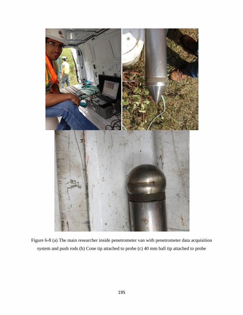
195
Figure 6-8 (a) The main researcher inside penetrometer van with penetrometer data acquisition
system and push rods (b) Cone tip attached to probe (c) 40 mm ball tip attached to probe

196
Figure 6-9 (a) 40 mm ball tip attached to penetrometer probe (b) 113 mm ball tip attached to
probe (c) Main researcher with 113 mm ball tip attached to penetrometer probe

197
Figure 6-10 (a) Penetrometer push rods being pulled out of the ground after completion of testing
(b) Penetrometer depth transducer box mounted onto drill rig to measure the push depth (c)
Different sizes of field (Nilcon) vanes

198
Figure 6-11 (a) Medium size vane attached to the vane push rod (b) Electronic vane motor
mounted on drilling augers and clipped to the vane push rods for testing (c) Drilling augers

199
Figure 6-12 (a) Piston sampler attached drill rig for undisturbed soil sampling by using shelby
tubes (b) Shelby tube attached to piston sampler with bags of sand and bentonite for sealing
around piezometer (c) Shelby tube with sample after just being pulled out from the ground (d)
Main researcher with undisturbed sample in a shelby tube

200
Figure 6-13 (a) Shelby tube being waxed and caped at the ends to prevent moisture transfer (b)
Flowing sensitive marine clay in Ottawa when disturbed (c) Screen attached at the end of tube
which is acting as a piezometer to measure the hydrostatic water pressure at different levels (d)
Piezometer tube being dropped into the ground to measure the hydrostatic water pressure

201
6.3 Appendix #3: Lab Graphs for Canadian Geotechnical Research Site
No. 1
Figure 6-14 (a) Consolidation graph at depth of 2.3 m (b) Consolidation graph at depth of 3.8 m
(c) Consolidation graph at depth of 16.8 m
0.5
0.7
0.9
1.1
1.3
1.5
1.7
8.00 800.00
Void
Ratio
Stress (kPa)
0.7
0.9
1.1
1.3
1.5
1.7
1.9
2.1
2.3
2.5
6 60 600
Void
Ratio
Stress (kPa)
0.8
0.9
1.0
1.1
1.2
1.3
1.4
1.5
1.6
1.7
1.8
5 50 500
Void
Ratio
Stress (kPa)

202
Figure 6-15 Grain size distribution for sample depths of 2.4 to 19.8 m
30
40
50
60
70
80
90
100
0.001 0.01 0.1 1 10
Passin
g [
%]
Grain Size [mm]
2.4
3.8
6.7
8.4
10.7
12.2
13.7
15.2
16.8
18.3
19.8
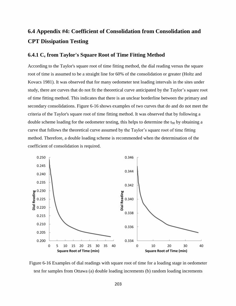
203
6.4 Appendix #4: Coefficient of Consolidation from Consolidation and
CPT Dissipation Testing
6.4.1 Cv from Taylor's Square Root of Time Fitting Method
According to the Taylor's square root of time fitting method, the dial reading versus the square
root of time is assumed to be a straight line for 60% of the consolidation or greater (Holtz and
Kovacs 1981). It was observed that for many oedometer test loading intervals in the sites under
study, there are curves that do not fit the theoretical curve anticipated by the Taylor’s square root
of time fitting method. This indicates that there is an unclear borderline between the primary and
secondary consolidations. Figure 6-16 shows examples of two curves that do and do not meet the
criteria of the Taylor's square root of time fitting method. It was observed that by following a
double scheme loading for the oedometer testing, this helps to determine the t90 by obtaining a
curve that follows the theoretical curve assumed by the Taylor’s square root of time fitting
method. Therefore, a double loading scheme is recommended when the determination of the
coefficient of consolidation is required.
Figure 6-16 Examples of dial readings with square root of time for a loading stage in oedometer
test for samples from Ottawa (a) double loading increments (b) random loading increments
0.200
0.205
0.210
0.215
0.220
0.225
0.230
0.235
0.240
0.245
0.250
0 5 10 15 20 25 30 35 40
Dia
l Re
adin
g
Square Root of Time (min)
0.334
0.336
0.338
0.340
0.342
0.344
0.346
0 10 20 30 40
Dia
l Re
adin
g
Square Root of Time (min)

204
6.4.2 Cv from Dissipation Testing
Campanella et al. (1988) performed CPTs with pore pressure dissipation by using different
positions of porous stone. Even though they had performed testing on sensitive marine clays in
western Canada rather than in eastern Canada, their conclusion may be useful for sensitive
marine clays in Ottawa. They observed that for overconsolidated soils, porewater pressure
measurements behind the tip and behind the sleeve friction exhibit an increase then decrease in
porewater pressure as a result of the gradient. They observed that this is not the case for
porewater pressure measurements at the tip. Therefore, the methods of interpretation and
estimating of the coefficient of consolidation only apply to the porewater pressure measurements
at the tip. However, measurements at the tip may be decreased as a result of stopping or
unloading of the tip. On the other hand, for normally consolidated or lightly overconsolidated
soils, porewater pressure measurements behind the tip and the sleeve mandrel are desirable
because they are not affected by the gradient and the unloading of the tip.
Pore pressure dissipation tests are available for Sites 1 and 7 and no oedometer tests are available
for these two sites for direct comparisons with the field pore pressure dissipation tests. However,
the coefficient of consolidation determined from these tests for these two sites are between
4.51x10⁻³
and 1.36x10⁻²
cm2/s which is outside and higher than the range determined from the
oedometer tests for all of the other sites as shown in Figure 6-17.
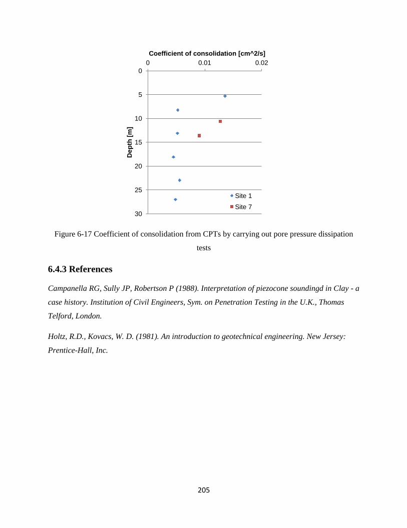
205
Figure 6-17 Coefficient of consolidation from CPTs by carrying out pore pressure dissipation
tests
6.4.3 References
Campanella RG, Sully JP, Robertson P (1988). Interpretation of piezocone soundingd in Clay - a
case history. Institution of Civil Engineers, Sym. on Penetration Testing in the U.K., Thomas
Telford, London.
Holtz, R.D., Kovacs, W. D. (1981). An introduction to geotechnical engineering. New Jersey:
Prentice-Hall, Inc.
0
5
10
15
20
25
30
0 0.01 0.02
Dep
th [
m]
Coefficient of consolidation [cm^2/s]
Site 1
Site 7