Auburn University

Department of Economics

Working Paper Series

Energy Tariffs, Production, and

Income in a Small Open Economy

Henry Thompson

Auburn University

AUWP 2013-11

This paper can be downloaded without charge from:

http://cla.auburn.edu/econwp/

http://econpapers.repec.org/paper/abnwpaper/

1

Energy Tariffs, Production, and Income in a Small Open Economy

Henry Thompson

Auburn University

May 2013

A tariff on imported energy in a small open economy alters production, redistributes income, and

generates tariff revenue. The present paper includes tariff revenue in a general equilibrium

economy producing two traded goods with imported energy and domestic capital and labor. An

energy tariff reduces energy intensive output and domestic factor income but payment to one

domestic factor may rise as might the other output. Tariff revenue, not included in the related

theoretical literature, is shown to be concave in the tariff. A simulation illustrates these general

equilibrium properties including the revenue maximizing tariff.

Keywords: Energy tariffs, tariff revenue, general equilibrium

Special thanks for discussions go to Leland Yeager and Andy Barnett as the present paper developed. Charlie Sawyer, Roy Ruffin, Tom Osang, Olena Ogrokhina, Alex Sarris, and George Chortoreas also provided useful comments. Contact information: Department of Economics, Auburn University AL 36849, 334-844-2910, thomph1@auburn.edu

2

Energy Tariffs, Production, and Income in a Small Open Economy

A tariff on an imported factor of production in a small open economy lowers the import,

shrinks the production frontier, and reduces domestic factor income. The present paper examines a

competitive economy producing two traded goods with imported energy and domestic capital and

labor, extending the theory by explicitly including tariff revenue. This model is the simplest that

addresses two underlying issues in the debate over energy tariffs, namely energy intensive output

and domestic factor income distribution.

If energy is an intensive factor for one of the goods, the tariff raises payment to the other

intensive factor but lowers payment to the middle factor. Output of the energy intensive good falls

but the other output may rise. Opposing interests in energy tariffs can be expected. Tariff revenue

is shown to be concave in the tariff, extending this property to a competitive general equilibrium

economy. A simulation illustrates these properties including the tariff that maximizes tariff revenue.

There is ample motivation for examining the effects of tariffs on energy imports. Energy

tariffs have one definite advantage over other taxes, offering governments a reliable source of

revenue when other taxes may be difficult to collect. Across energy importing countries, tariff

revenue maximization may be a common policy goal. Kline and Weyant (1982) make the point that

energy tariffs have the advantage of reducing dependence in importing countries, but their negative

economic impacts are documented by Hebatu and Semboja (1994).

Energy tariffs in the form of border carbon taxes would facilitate reaching carbon dioxide

emission targets. Proost and Regemorter (1992) find tariffs on embodied carbon dioxide are

effective in attaining abatement targets. Dissou and Eyland (2011) find tariffs are effective but at a

higher cost than emission taxes, while Böhringer, Bye, Fæ hn, and Rosendahl (2012) find tariffs

3

compare more favorably. The higher domestic price resulting from an energy tariff also substitutes

for alternative energy subsidies.

The present paper does not include any externality but contributes with a general

equilibrium model that separates energy intensive production, allows redistribution of domestic

factor income, and includes tariff revenue in income. Effects on the pattern of production and

income distribution are central if underlying issues in the political debate surrounding energy tariffs.

The first section introduces the general equilibrium of the small open economy followed by a

section that develops the comparative static model. The third section provides model background

on domestic factor endowments and product prices. The fourth section analyzes the effects of an

energy tariff on energy imports, outputs, domestic factor prices, and income. A final section

simulates a Cobb-Douglas economy across a range of energy tariffs, illustrating the tariff that

maximizes revenue.

1. Factor tariffs, output, and income

Imported energy input is an example of an internationally mobile factor of production

introduced by Mundell (1957) to the theory of production and trade in a small open economy. This

literature, focusing on exogenous changes in the world price of the imported factor, includes Kemp

(1966), Jones (1967), Chipman (1971), Caves (1971), Jones and Ruffin (1975), Ferguson (1978),

Srinivasan (1983), Svensson (1984), Fergusen (1978), Thompson (1983), and Ethier and Svensson

(1986). The present paper extends this theory by explicitly considering an input tariff and including

tariff revenue in income distribution.

There is a related literature on imported intermediate goods entering production with fixed

unit inpu coefficients. Ruffin (1969) develops the fundamentals model of utility maximization with a

4

tariff on an imported intermediate good. Panagaria (1992) finds the tariff has an ambiguous utility

effect. In the present model, this ambiguous effect would be weakened due to the substitution of

domestic factors for imported energy with the tariff.

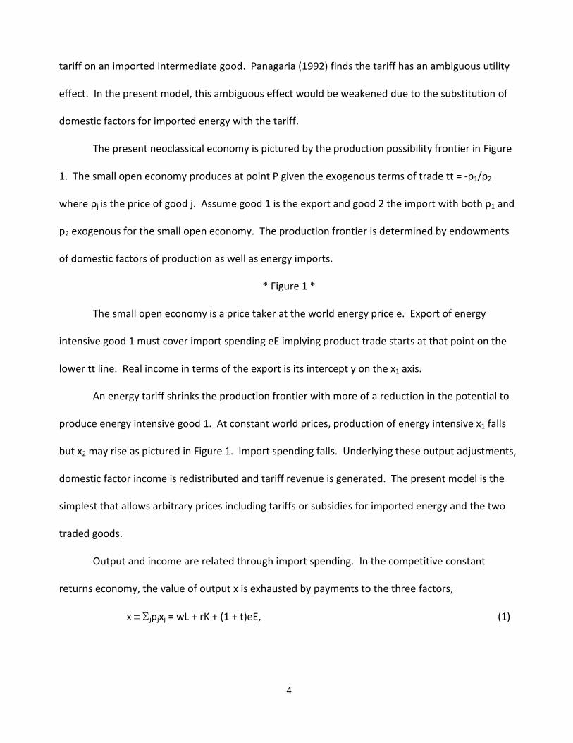
The present neoclassical economy is pictured by the production possibility frontier in Figure

1. The small open economy produces at point P given the exogenous terms of trade tt = -p1/p2

where pj is the price of good j. Assume good 1 is the export and good 2 the import with both p1 and

p2 exogenous for the small open economy. The production frontier is determined by endowments

of domestic factors of production as well as energy imports.

* Figure 1 *

The small open economy is a price taker at the world energy price e. Export of energy

intensive good 1 must cover import spending eE implying product trade starts at that point on the

lower tt line. Real income in terms of the export is its intercept y on the x1 axis.

An energy tariff shrinks the production frontier with more of a reduction in the potential to

produce energy intensive good 1. At constant world prices, production of energy intensive x1 falls

but x2 may rise as pictured in Figure 1. Import spending falls. Underlying these output adjustments,

domestic factor income is redistributed and tariff revenue is generated. The present model is the

simplest that allows arbitrary prices including tariffs or subsidies for imported energy and the two

traded goods.

Output and income are related through import spending. In the competitive constant

returns economy, the value of output x is exhausted by payments to the three factors,

x jpjxj = wL + rK + (1 + t)eE, (1)

5

where pj is the price of good j, L is the labor endowment, K is the capital endowment, w is the wage,

r is the capital return, e is the price of imported energy, E is the level of energy import, and t is the

energy tariff. Factors are paid marginal products in each sector.

Income y is domestic factor payment plus tariff revenue,

y rK + wL + teE, (2)

equivalent to output less import spending y = x – eE due to the competitive factor markets. An

increase in the tariff t lowers imports E as factor prices r and w adjust.

The effects of the tariff depend on the two production functions reflected in the comparative

static model by factor shares of sector revenue, industry shares of factor employment, and

substitution elasticities between the three factors. Tariff effects also depend on levels of domestic

factor endowments, output prices facing the small open economy, and the level of the tariff itself.

2. The comparative static model with imported energy

Imported energy is utilized according to E = jaEjxj in the two sectors j = 1, 2 where aEj is the

cost minimizing energy input per unit of output j. By Shepard’s lemma aEj is the partial derivative of

the cost function with respect to energy input. The neoclassical constant returns production

functions have positive and diminishing marginal products.

Energy

imports change according to dE = j(aEjdxj + xjdaEj) or in elasticity form,

E = jEj(aEj + xj), (3)

where primes denote percentage changes and industry utilization or employment shares Ej

aEjxj/E sum to one. Given constant returns, the homogeneous unit energy inputs aEj depend only on

relative factor prices. Employment conditions for domestic capital and labor are similar to (3).

6

Energy imports E are endogenous in the model while domestic factor endowments K and L are

exogenous.

Given the exogenous world energy price e, the domestic price eD (1 + t)e changes

according to deD = edt. The model focuses on the percentage change in the domestic price eD due

to a tariff,

≡ dt/(1 + t). (4)

Substitution elasticities capture adjustments in the cost minimized factor mix terms to

changing factor prices. As an example, the cross price substitution elasticity of capital relative to the

domestic price of energy KE jKj(aKj/) is the industry share weighted sum of cross price

elasticities.

Capital may be a complement relative to the price of energy as found by Berndt and Wood

(1975). In the present context, the energy tariff would lower capital input per unit of output

reducing capital demand and strongly increasing labor demand. Griffin and Gregory (1976) find

instead that capital substitutes for energy, suggesting increased capital demand due to an energy

tariff and less of an increase in the demand for labor. The literature on the substitution of capital

with respect to the price of energy is reviewed by Thompson (2006).

In the present two sector model, production functions differ between sectors raising the

possibility of capital as a complement with energy in one sector but a substitute in the other. Factor

intensity of the two sectors is critical to the adjustment process, as are the sizes of the sectors.

Adjustments of outputs and domestic factor prices interplay in the general equilibrium. Potential

adjustments to the energy tariff expand considerably with the possibility of complements in

production.

7

Own substitution elasticities, describing sensitivity of unit inputs to their own prices, are

negative. Linear homogeneity implies elasticities for each input across factor prices sum to zero, iE

+ iL + iK = 0 where i = K, L, E. If capital is a complement with respect to the domestic price of

energy, KE and EK are negative. Concavity implies own effects outweigh cross effects, iikk - ikki

> 0 for i, k = K, L, E.

Unit energy inputs adjust according to aEj = EKr + ELw + EE expanding adjustment in

energy imports in (3) to

E = EKr + ELw + EE + jEjxj. (5)

Adjustments to changes in exogenous endowments of domestic capital K and labor L are similar.

Revenue in a sector is exhausted by payments to the three factors, pjxj = wLj + rKi + (1 + t)eEj

for j = 1, 2. Divide by output xj to link the output price to the three factor prices, pj = eDaEj + waLj +

raKj. Differentiate to find dpj = eaEjdt + aLjdw + aKjdr + [eDdaEj + wdaLj + rdaKj]. The bracketed

expression disappears due to the cost minimizing envelope property leading to the competitive

pricing condition in elasticity form

pj = θEj + θKjr + θLjw, (6)

where the θij are factor shares of the revenue and iθij = 1.

Income y = rK+ wL + teE in (2) changes according to dy = rdK + wdL + Kdr + Ldw + tedE + eEdt.

In elasticity form

y = K(K + r) + L(L + w) + R(E + T), (7)

where T (1 + t)/t and the three income shares K rK/y, L wL/y, and R teE/y sum to one.

Tariff revenue R teE and its share R of income have not been included in the literature on

international factor mobility.

8

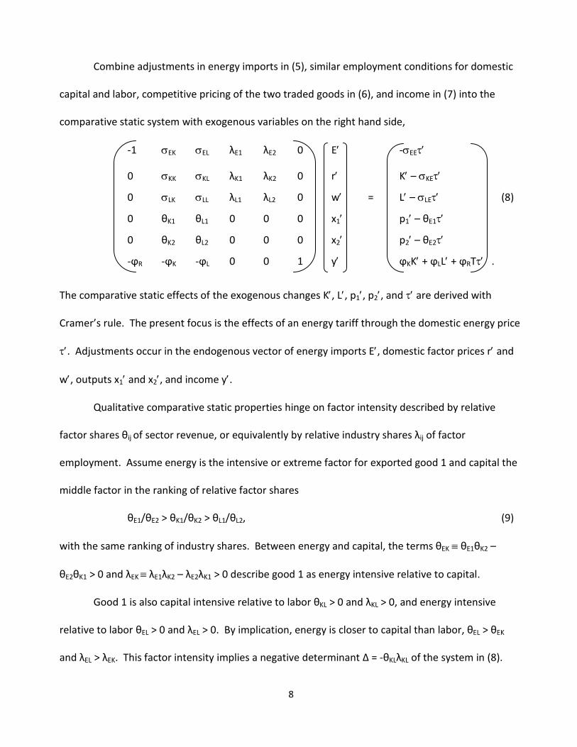
Combine adjustments in energy imports in (5), similar employment conditions for domestic

capital and labor, competitive pricing of the two traded goods in (6), and income in (7) into the

comparative static system with exogenous variables on the right hand side,

-1 EK EL λE1 λE2 0 E -EE

0 KK KL λK1 λK2 0 r K – KE

0 LK LL λL1 λL2 0 w = L – LE (8)

0 θK1 θL1 0 0 0 x1 p1 – θE1

0 θK2 θL2 0 0 0 x2 p2 – θE2

-ϕR -ϕK -ϕL 0 0 1 y ϕKK + ϕLL + ϕRT .

The comparative static effects of the exogenous changes K, L, p1, p2, and are derived with

Cramer’s rule. The present focus is the effects of an energy tariff through the domestic energy price

. Adjustments occur in the endogenous vector of energy imports E, domestic factor prices r and

w, outputs x1 and x2, and income y.

Qualitative comparative static properties hinge on factor intensity described by relative

factor shares θij of sector revenue, or equivalently by relative industry shares λij of factor

employment. Assume energy is the intensive or extreme factor for exported good 1 and capital the

middle factor in the ranking of relative factor shares

θE1/θE2 > θK1/θK2 > θL1/θL2, (9)

with the same ranking of industry shares. Between energy and capital, the terms θEK θE1θK2 –

θE2θK1 > 0 and λEK λE1λK2 – λE2λK1 > 0 describe good 1 as energy intensive relative to capital.

Good 1 is also capital intensive relative to labor θKL > 0 and λKL > 0, and energy intensive

relative to labor θEL > 0 and λEL > 0. By implication, energy is closer to capital than labor, θEL > θEK

and λEL > λEK. This factor intensity implies a negative determinant Δ = -θKLλKL of the system in (8).

9

There are six possible factor intensity rankings, each with its own signs of θik and λik terms for

i, k = K, L, E. Comparative static properties are sensitive to the intensity ranking. The critical

alternative assumption is that energy is the middle factor as in θK1/θK2 > θE1/θE2 > θL1/θL2, leading to

qualitatively different comparative static effects discussed in the results.

3. Changes or differences in endowments and prices

This section presents model background on factor endowments and output prices. Changes

or differences in domestic factor endowments affect energy imports in (8) according to E/K =

λEL/λKL > 0 and E/L = -λEK/λKL < 0. Increased endowment of middle factor capital raises energy

imports while increased endowment of labor, intensive in the other sector, reduces energy imports.

Energy imports are independent of substitution due to the lack of any factor price impacts in

the factor price equalization property noted below. In other models with less aggregated inputs and

outputs, substitution would have some influence on adjustments in energy imports to changes in

domestic endowments. Projecting these comparative static results to compare two economies that

are otherwise identical, the capital abundant one would import more energy,

If energy is the middle factor, the negative λEK implies energy imports increase with both K

and L endowments. Comparing two such economies, if energy were closer to capital in intensity in

the property -λEK > λEL then the capital abundant country would import more energy.

The factor price equalization property holds with adjustments in factor demands exactly

offsetting changes in factor supplies, w/L = r/L = w/K = r/K = 0. Factor price equalization is

characteristic of models such as the present one with the same number of factors and exogenous

prices. Trade between two such economies based on different domestic factor endowments would

lead to equal factor prices.

10

Outputs follow factor intensity in Rybczynski type endowment effects. Each output has a

positive link to the endowment of its intensive domestic factor and a negative link to the other.

Good 1 output increases with capital, and good 2 with labor. Ruffin (1977) develops the comparison

of two such economies with trade following the Heckscher-Ohlin pattern based on factor abundance

and intensity.

Domestic factor endowments affect income according to

y/K = ϕK + ϕRλEL/λKL > 0 (10)

y/L = ϕL – ϕRλEK/λKL.

Income shares affect the direction and size of these factor endowment effects. An increase in

capital raises income by its return, attracting energy and raising tariff revenue. The total adjustment

y/K is the income weighted average of these two positive effects.

An increase in labor raises income by the wage but lowers energy imports and tariff revenue

leading to its ambiguous effect on income. A positive effect of labor on income is favored by a

larger labor share of income, as well as capital close to energy in factor intensity.

If energy is the middle factor, the positive λEK implies both capital and labor raise income. If

capital and labor are more similar in factor intensity λKL becomes smaller and domestic factor

endowments have larger effects on income.

The effects of changing prices on energy imports depend on substitution as well as intensity.

For a change in the price of good 1,

E/p1 = (θK2σ1 – θL2σ2)/, (11)

where σ1 λKLσEL – λELσKL + λEKσLL = (λKL – λEK)σEL – (λEL + λEK)σKL and σ2 λKLσEK – λELσKK + λEKσLK = (λKL +

λEL)σEK + (λEK + λEL)σLK. There is a presumption that σ1 < 0 and σ3 > 0 implying E/p1 > 0 with an

11

increase in the price and output of energy intensive good 1 raising energy imports. Energy imports

could decrease, however, if energy is a strong substitute for labor with a large positive σEL and a

complement with capital with a negative σEK. This unusual result is also favored by a large intensity

difference between capital and labor in a large λKL term. A change in p2 is similar with the

presumption that E/p2 = (-θK1σ1 + θL1σ2)/ < 0. Thompson (1983) shows imports must increase

with at least one of the two product prices. In the present model, the strong presumption is that

imports increase with the price of the energy intensive good.

Standard Stolper-Samuelson adjustments of domestic factor prices to changing product

prices depend only on factor intensity. The production frontier is also locally convex in prices with

xm/pn cofactors that are determinants of two factor production models.

A change in the price of good 1 affects income according to y/p1 = [(ϕKθL2 – ϕLθK2)/θKL] +

ϕR(E/p1). The expression in brackets is positive due to the spanning condition for full employment,

K/L > K2/L2, implying a net positive effect of an increase in p1 on domestic factor payments. A larger

income share ϕR of tariff revenue and increase in energy imports favor increased income. Analysis

of a change in p2 is similar with an ambiguous outcome due to falling energy imports.

4. Adjustments to an energy tariff

An energy tariff lowers imports in (8) according to

E/ = -Δ32/Δ < 0, (12)

where Δ32 is the negative determinant of the model with three domestic factors. Concavity of the

two production functions implies Δ32 < 0 as discussed by Chang (1979) and Thompson (1985). This

mutatis mutandis downward sloping import demand is not apparent given the flexibility of the two

outputs and two domestic inputs.

12

Elastic energy demand E/ < -1 follows if -Δ32 < -Δ in a condition favored by stronger

substitution. If energy demand is elastic, the tariff reduces import spending inclusive of the tariff.

Weaker substitution would lead to inelastic energy import demand.

Effects of the energy tariff on domestic factor prices depend only on factor intensity,

r/ = -θEL/θKL < 0 (13)

w/ = θEK/θKL > 0.

Domestic factors have polar interests in an energy tariff with middle factor capital hurt while

intensive labor benefits. Rising wages are consistent with expanding labor intensive output as the

economy shifts away from energy intensive production. If energy were the middle factor, the

negative θEK would imply both domestic factor prices fall with the tariff.

The energy tariff shrinks the production frontier as the two outputs adjust according to

x1/ = (λK2σ3 + λL2σ4)/ (14)

x2/ = -(λK1σ3 + λL1σ4)/,

where σ3 θELσLK – θKLσEL + θEKσLL = θELσLK – (θKL + θEK)σEL – θEKσKL and σ4 θKLσEK – θELσKK – θEKσKL =

(θKL + θEL)σEK + θKLσLK – θEKσKL Both factor intensity and substitution affect these output adjustments

with the presumption that σ3 < 0 and σ4 > 0.

The tariff must lower at least one of the two outputs as shown by Thompson (1983). Energy

intensive output x1 is presumed to fall as in Figure 1. An increase in labor intensive output x2 is

consistent with the rising wage w in (13).

If energy and capital were complements, the negative substitution elasticities σLK and σKL

would favor a positive σ3 and less of a decrease in x1 due to the tariff. The higher domestic price of

energy reduces the unit capital input with strong substitution toward labor, leading to the smaller

13

decrease in x1. A smaller share of capital employed in sector 1 reflected by a larger λK2 also favors

less of a decrease in energy intensive output x1.

Income adjusts to the energy tariff according to

y/ = [ϕL(w/) + ϕK(r/)]/θKL + ϕE(R/), (15)

where tariff revenue is R teE and R/ = T + E/. The first two terms in (15) simplify to (ϕLθEK –

ϕKθEL)/θKL reflecting the rising wage and falling capital return in (13). Direct substitution implies

ϕLθEK < ϕKθEL implying the tariff lowers domestic factor income.

A larger labor share ϕL favors less of a decrease in domestic factor income due to the

increased weight on the rising wage. A larger θEK and smaller θEL also favor less of a decrease in

domestic factor income with energy closer to labor in factor intensity.

The term ϕR(R/) = ϕR(T + E/) in (15) captures the adjustment in tariff revenue. An

increase in the tariff lowers the term T = (1 + t)/t offsetting the decreased import. At lower tariffs T

is high and tariff revenue R rises with the tariff. At higher tariffs T approaches 1 and the negative

E/ becomes more elastic.

At higher tariffs, the tariff lowers tariff revenue R. Substitution elasticities also become

stronger at higher tariffs implying a more elastic E/. As a result the tariff lowers revenue at higher

tariff levels. The following simulation illustrates concave tariff revenue with Cobb-Douglas

production.

5. A simulated energy tariff

Consider the general equilibrium adjustments to a range of energy tariffs from 0 to 1 with

Cobb-Douglas production functions. For energy intensive sector 1 the production function is x1 =

K10.5L1

0.2E10.3 and for the labor intensive sector x2 = K2

0.4L20.5L2

0.1. Factor intensity maintains the

14

ranking in (9) throughout the range of tariffs as industry shares adjust. Cobb-Douglas is a familiar

but restrictive functional form with constant factor shares but simulations with constant elasticity

and translog production functions produce similar results.

Fully employed domestic factor endowments are K = 100 and L = 10. The price e of imported

energy and prices p1 and p2 of the two goods are standardized to 1. Factor endowments are chosen

to be consistent with prices and production functions for feasible economic results across the range

of tariffs. Adjustment paths to the rising tariff are not overly sensitive to changing parameters

except for the Cobb-Douglas production coefficients.

The main behavioral assumptions are full employment and competitive pricing with factors

paid marginal products in each sector. These constraints motivate the nonlinear optimization of

income y = wL + rK + teE. Due to Euler’s theorem, optimization of y = p1x1 + p2x2 – E yields the

identical outcome.

Figure 2 plots adjustments to a tariff rising from 0 to 1. Energy imports E declines by 83%

from 8.3 at t = 0 to 1.4 at t = 1. Energy intensive output x1 declines from 26.6 to 3.4 across the range

of tariffs, as labor intensive x2 increases from 3.4 to 17.4. Total output x = x1 + x2 declines by 31%

from 30.0 to 20.8. These substantial adjustments in energy imports and outputs are characteristic

of the constant factor shares in Cobb-Doublas production. Stronger constant elasticity substitution

leads to a declining energy share with less of a decline in imports and smaller output adjustments.

* Figure 2*

Income y declines 11% from 21.7 to 19.4 across the range of tariffs. Income becomes more

sensitive to the tariff as the rate increases with the income elasticity y/ in (15) falling from -0.004

to -0.242. At higher domestic energy prices, income is more exposed to the increased domestic

15

price of energy. At low tariffs, the reduced energy import spending nearly offsets falling domestic

factor income. The effect of the tariff on income is weaker with stronger constant elasticity

substitution.

Figure 3 shows the associated change in domestic factor payments due to the rising energy

tariff. The capital payment rK declines 41% from 14.7 to 8.6 as the labor payment wL increases 34%

from 7.0 to 9.4 across the range of tariffs. A higher energy tariff would always be favored by labor

although total domestic factor payment declines 17% from 21.7 to 18.0 across the range of tariffs.

* Figure 3 *

Tariff revenue R rises from 0 to its maximum 1.62 at tR = 0.59, the tariff of a revenue

maximizing government. The tariff revenue share ϕR of income has a similar path that is maximized

at tϕ = 0.64, with the negative effect of the tariff on domestic factor payment implying tϕ > tR.

Stronger constant elasticity substitution results in a higher revenue maximizing tariff.

The elastic effect of the tariff on energy imports E/ becomes stronger as the tariff

increases, falling from -2.16 to -3.33 over the range of tariffs. Energy imports become more elastic

at higher tariff levels. Stronger constant elasticity substitution leads to less elastic energy imports.

The effect of the tariff on the domestic energy price diminishes as the tariff increases with

falling from 0.010 to 0.005 over the range of tariffs. The marginal effect of tariff revenue on income

M ≡ ϕE(T + E/) from (15) declines and becomes negative in Figure 3 at the revenue maximizing

tariff tR.

The energy import tariff can be analyzed in addition to other taxes. For instance, if the

government taxes factor income at 10% government revenue rises from g = 2.2 at t = 0 to its

16

maximum g* = 3.5 at tg = 0.52. The negative effect of the energy tariff on domestic factor payments

implies tg < t*. A similar result follows with output taxes.

6. Conclusion

Other issues regarding energy tariffs can be mentioned. An energy tariff for a large economy

lowers the international price. Weitzel, Hübler, and Peterson (2012) stress oil tariffs as a strategic

tool to affect the terms of trade. A Metzler (1949) paradox with a lower domestic energy price

inclusive of the tariff is feasible and perhaps likely in the global oil market as described by Thompson

(2007).

For an economy with domestic energy supply competing with the import, the tariff would

increase quantity supplied. This increase in the domestic resource payment could result in higher

income. Jones (1990) documents the positive effect of an oil tariff on US oil output and income.

The present adjustments to an energy tariff depend on production functions, domestic factor

endowments, income shares, and the tariff level. An energy tariff lowers imports and shrinks the

production frontier. Payment to the domestic factor intensive in the other sector rises as might the

other output, while payment to the middle domestic factor falls. If energy is the middle intensity

factor, a tariff lowers both domestic factor prices. At least one of the two outputs must fall with the

tariff. These results suggest unanimous political opinion on energy tariffs cannot be expected.

There may be an energy tariff that maximizes tariff revenue. For many governments, the

implicit goal of revenue maximization suggests the present model is relevant for predicting energy

tariffs.

17

References

Bemdt, Ernst, and Laurits Christensen (1973) The internal structure of functional relationships:

Seperability, substitution, and aggregation, The Review of Economic Studies 55, 403-10.

Böhringer, Christoph Brita Bye, Taran Fæ hn, and Knut Einar Rosendahl (2012) Alternative designs for

tariffs on embodied carbon: A global cost-effectiveness analysis, Energy Economics 34, 143-53.

Caves, Richard (1971) International corporations: The industrial economics of international

investment, Economica 38, 1-27.

Chang, Winston (1979) Some theorems of trade and general equilibrium with many goods and

factors, Econometrica 47, 790-26.

Chipman, John (1971) International trade with capital mobility: a substitution theorem, in Trade,

Balance of Payments, and Growth, edited by Jagdish Bhagwati, Ron Jones, Robert Mundell, and

Jaroslav Vanek, North Holland.

Dissou, Yazid and Terry Eyland (2011) Carbon control policies, competitiveness, and border tax

adjustments, Energy Economics, 33, 556-64.

Ethier, Bill and Lars Svensson (1986) The theorems of international trade and factor mobility, Journal

of International Economics 20, 21-42.

Ferguson, David (1978) International capital mobility and comparative advantage: The two-country,

two-factor case, Journal of International Economics 8, 373-96.

Griffin, James and Paul Gregory (1976) An intercountry translog model of energy substitution

responses, American Economic Review 66, 845-57.

Hatibu Haji and Haji Semboja (1994) The effects of energy taxes on the Kenyan economy: A CGE

analysis, Energy Economics 16, 205-15.

Jones, Clifton (1990) An oil import fee and drilling activity in the USA: A comment, Energy Economics

4, 302-4.

Jones, Ron (1967) International capital movements and the theory of tariffs and trade, Quarterly

Journal of Economics 81, 1-38.

18

Jones, Ron and Roy Ruffin (1975) Trade patterns with capital mobility, in Current Economic

Problems, edited by M. Parkin and A. Nobay, Cambridge.

Kemp, Murray (1966) The gains from international trade and investment: A neo-Heckscher-Ohlin

approach, American Economic Review 56, 788-809.

Kline, David and John Weyant (1982) Reducing dependence on oil imports, Energy Economics 4, 51-

64.

Metzler, Lloyd (1949) Tariffs, international demand, and domestic prices, Journal of Political

Economy 57, 345-51.

Mundell, Robert (1957) International trade and factor mobility, American Economic Review 47, 321-

35.

Panagariya, Arvind (1992) Input tariffs, duty drawbacks and tariff reforms, Journal of International

Economics 26, 132-47.

Proost, S. and D. Van Regemorter (1992) Economic effects of a carbon tax: With a general

equilibrium illustration for Belgium, Energy Economics 14, 136-49.

Ruffin, Roy (1969) Tariffs, intermediate goods, and domestic protection, American Economic Review

49, 261-9.

Ruffin, Roy (1977) A note on the Heckscher-Ohlin theorem, Journal of International Economics 7,

403-5.

Srinivasan, T.N. (1983) International factor movements, commodity trade and commercial policy in a

specific factors model, Journal of International Economics 12, 389-12.

Svensson, Lars (1984) Factor trade and goods trade, Journal of International Economics 16, 365-78.

Thompson, Henry (1983) Trade and international factor mobility, Atlantic Economic Journal 11, 45-8.

Thompson, Henry (1985) Complementarity in a simple general equilibrium production model,

Canadian Journal of Economics 18, 616-21.

19

Thompson, Henry (2006) The applied theory of energy substitution in production, Energy Economics, 28, 410-25.

Thompson, Henry (2007) Oil depletion and terms of trade, Keio Economic Studies, 19-25

Weitzel, Matthias, Michael Hübler, and Sonja Peterson (2012) Fair, optimal or detrimental?

Environmental vs. strategic use of border carbon adjustment, Energy Economics 34, 198-207.

20

x2

x1

tt

eE

P

Figure 1. A factor tariff and income

y

21

Figure 2. Outputs, import, and income

Figure 3. Factor payments and tariff revenue

0

5

10

15

20

25

30

0 0.1 0.2 0.3 0.4 0.5 0.6 0.7 0.8 0.9 1

x1 x2 E x-E

-1

1

3

5

7

9

11

13

15

0 0.1 0.2 0.3 0.4 0.5 0.6 0.7 0.8 0.9 1

rK wL R M