determinants of income distribution in the nigeria economy

ISSN 1923-841X [Print]ISSN 1923-8428 [Online]

www.cscanada.netwww.cscanada.org

International Business and ManagementVol. 5, No. 1, 2012, pp. 126-137DOI:10.3968/j.ibm.1923842820120501.1020

126Copyright © Canadian Research & Development Center of Sciences and Cultures

Determinants of Income Distribution in the Nigeria Economy: 1977-2005

A.A. Awe[a],*; Olawumi Ojo Rufus[a]

[a]Department of Economics, Ekiti State University Ado-Ekiti, Nigeria.*Corresponding Author. Address: Department of Economics Ekiti State University, Ado-Ekiti, Nigeria.

Received 19 June 2012; Accepted 30 July 2012

AbstractThe study carried out an investigation of a number of factors which determine income distribution in Nigeria by making empirical analysis of the relationship between the determinants and income distribution using the co-integration technique. The empirical findings in the study revealed that, Gini Coefficient is very high in Nigeria, indicating a high level of income inequality. Also, employment rate, inflation rate, Gross Domestic Product and social spending were true determinants of income distribution in the Nigerian economy during the period under review (1977-2005). The study also found that, both the growth rate of output and government health expenditure exhibited an inverse relationship with Gini coefficient of income distribution in the Nigerian economy while employment rate, inflation rate and government education expenditure had direct relationship with Gini coefficient of income distribution in the Nigerian economy. Moreso, the findings showed the existence of a long run relationship between income distribution and its determinants in Nigeria. Finally, from the empirical findings in this research work and based on the relationship each determinant exhibited with the Gini coefficient of income distribution in Nigerian economy, a set of policy recommendations were made such as: government ensuring the formulation and implementation of more pragmatic employment policies in Nigeria, government ensuring proper monitoring of its spending on education and health through appropriate policy measures and policies that bring about more equitable distribution of income and associated income earning opportunities were suggested among others.

Key words: Income distribution; Inegquate; Gini coefficient enploment rate; Nigeria economy

A.A. Awe, Olawumi Ojo Rufus (2012). Determinants of Income Distribution in the Nigeria Economy: 1977-2005. International Business and Management, 5 (1), 126-137. Available from: URL: http://www.cscanada.net/index.php/ibm/article/view/j.ibm.1923842820120501.1020 DOI: http://dx.doi.org/10.3968/j.ibm.1923842820120501.1020

INTRODUCTIONIncreasing income inequality and poverty continue to be the most challenging economic trend facing most developing countries, particularly Nigeria. There are enough evidences to show that poverty and income inequalities are on the increase. For instance, Canagarajah, et al. (1997), reported increased level of poverty over the period spanning the 1980s and 1990s in Nigeria. The study further revealed high level of income inequality over the same period. This inequality was established by an increase in Gini coefficient from 38.1 percent in 1985 to 44.9 percent in 1992.

The Nigerian economy is characterized by a large rural agricultural-based traditional sector that encompasses about two-third of the population in the low-income class. Most of these people at the bottom of the income distribution chart are living in abject poverty (Canagarajah et al., 1997). Also, a high rate of unemployment and under employment, a large public sector, low wage and poor working conditions characterized the labour market in Nigeria. Also, varying degree of income inequality compounded by a keen middle class has continued to exhibit a strong influence on the nature and pattern of income distribution in the Nigerian economy (Alayande, 2003).

In the 1960s and 1970s, the Nigerian economy provided jobs for its teeming population and absorbed considerable imported labour in the key sectors of the economy. The wage rate which dictated the income level

A.A. Awe; Olawumi Ojo Rufus (2012). International Business and Management, 5(1), 126-137

127 Copyright © Canadian Research & Development Center of Sciences and Cultures

competed favourably with international standard and there was relative industrial peace in the whole economy (Nnnanna et al., 2003). Following the oil boom of the 1970s, there was mass migration of people, especially the youth to the urban areas seeking for jobs. This movement worsened the employment situation in the urban areas as the employers of labour found it difficult to accommodate this massive influx of rural dwellers who are mostly youths. The reason however, was not unconnected with the shortage of funds to pay the income of the prospective job seekers. However, following the downturn in the economy in the 1980’s, the problem of unemployment started to manifest, precipitating the introduction of the Structural Adjustment Programme (SAP), the rapid depreciation of the naira exchange rate and inability of most industries to import raw materials required to sustain their output levels (Nnnanna et al., 2003).

A major consequence of the rapid depreciation of the naira after SAP was the sharp rise in the general price level, leading to a significant decline in the real income. The low income inturn aggravated a weakening purchasing power of income earners and declining aggregate demand. Consequently, industries started to accumulate unintended inventories and all sectors in the economy started to rationalize their work force thereby compounding the problem of unemployment and income inequality in the country. As a corollary to this, the public sector of the Nigerian economy places an embargo on employment due to lack of the required capacity to pay their income. With the simultaneous rapid expansion in educational sector, new entrants into the labour market increased beyond the absorptive capacity of the economy. Thus the avowed government objective of achieving full employment failed to materialize.

Income distribution is central to the development of any nation. This simply explains the popularity which issues on income distribution have gained among various scholars in Economics. Income distribution has become a contemporary issue in the developing economies which has enjoyed the patronage of some researchers such as Aboyade (1978), Fajana (1985), Deininger and Squire (1996), Bulir (2001), Rossana and Hoeven (2001), Jose and Teilings (2002), Alayande (2003), Ogwumike et al. (2003), Dodson (2005), Awoyemi (2005), Jones (2007), Oguntuase (2007), among others who have contributed to the concept of income distribution. For instance, Fajana (1985) expressed employment rate as an important determinant of income distribution using Nigeria data. He employed the Ordinary Least Square technique of analysis of established the nexus between the variables.

In the same vein, Deininger and Sqaure (1996) expressed number of declared vacancies as a determinant of income distribution and relied on the Ordinary Least Square method of analysis to establish the nexus between the variables. Jose and Teilings (2002) in their view, expressed the Gini coefficient of income distribution as

a function of a number of explanatory variables such as; employment rate, education, government social, inflationary rate, GDP per capita and percentage of old people above sixty years using the Ordinary Least Square method of estimation. In congruence to the view of Jose and Teilings (2002), Oguntuase (2007) in an empirical study on the determinants of income distribution in the manufacturing sector of the Nigerian economy, expressed Gini coefficient of income distribution as a function of employment rate, literacy rate (proxy for education), inflationary rate and manufacturing sector share of the GDP. He made use of the cointegration analysis and the Error Correction Model to establish the nexus among the variables.

However, considering critically the various views earlier explained, the major question that arises is; what is the long-run relationship that existed among the variables? It was observed that none of these views explained the time series properties of the variables, which may help to determine whether there is a long run relationship among the variables in the Nigerian economy. Only Oguntuase (2007) who delved into the verification of the long-run relationship among income distribution and some explanatory variables focused on the manufacturing sector of the Nigerian economy. A sectoral appraisal of the determinants of income distribution is only a means to an end and not an end in itself. Therefore, the study is set to fill the missing gaps created by past researchers. Firstly, by incorporating variables which represents the existing views on determinants of income distribution; secondly, by assessing the long-run relationship among the variables; which past researchers emphasized.

1. REVIEW OF EMPIRICAL WORKSMajor studies on income distribution centered on descriptive method of analysis, various results of surveys on income distribution were compiled by different authors in the past. Income distribution has been seen summarily as the pattern of earnings of the rich and the poor in any economy. One of the earliest works on income distribution is the Kuznet’s hypothesis by Professor Kuznet. He was the first economist to study income distribution empirically. In his 1955 study, it was revealed that in LDCs 60% of the poorest received 30% and less of national income, whereas in DCs, they received more than 30% of national income. So far as the richest 20% in LDCs are concerned, they received 50% and more of national income. In DCs, they received 45% and less. Kuznet (1955) came to the conclusion that, the size distribution income was more unequal in LDCs than in DCs. It was high (1.67 to 2.33) in LDCs and low (1.25 to 1.29) in DCs.

Also Kuznet (1963) developed an inverted U-shaped hypothesis by taking the data of 18 countries by size distribution of income, from where he constructed



different Lorenz curves for DCs and derived their Gini coefficient. It was 0.37 percent for DCs and 0.44 percent for LDCs. It showed that income inequalities were higher in LDCs than DCs. This was explained in the graph of Lorenz curve in figure 2.1 above, where the 45° straight line OD is of equal income distribution, the thick curve to the right and nearest to this line is the Lorenz curve of developed countries (DCs). The dotted curve further to the right represented the Lorenz curve of less Developed Countries (LDCs). However, Kuznet’s study was criticized based on the fact that he took average small sample of developing and developed countries. Todaro (2000) maintains that Kuznet’s analysis was based on 5% empirical information and 95% speculation.

Based on the forgoing, some authors that followed Kuznet have tried to narrow down the scope by focusing on one or two economies for the basis of their studies. One of these is the research work on income distribution and employment in Nigerian urban sector by Fajana (1985). Aboyade and Yakubu acknowledge the good empirical work of Fajana titled, “the empirical analysis of the relationship between differential in earnings of employed and employee power in some selected manufacturing firms in Nigeria”. He focused on differential in earnings (income distribution). Fajana captured income distribution by using four categories of employee’s earnings and assessed the impact of employee’s power (employment rate) of an industry on each of them. Average earnings of employees were divided into earnings of clerical officer, manual/casual operatives (junior employee), professional and managerial employees (senior employees). After critical analysis of this model and concluding from his findings, Fajana (1985), logically deduced that casual factors of the differences in labour power i.e. employment rate constitutes an integral part of the explanatory hypothesis for inter industry wage differentials in Nigeria.

Moreover, Adesimi (1990) analyzed the structure of rural-urban income distribution vis-à-vis occupational group, and conducted a survey of the four major states in the western part of the country that is, Lagos, Ogun, Ondo and Oyo. The economy was divided into rural and urban sector which has been weighted and scored for the divisions on the basis of population, major economic activity, services and level of industrialization. He observed that the rural sector received 38.3% of the tax payers income in the three states of Oyo, Ondo and Ogun for which data are available.

The reason for this lopsided distribution between the urban and the rural sectors are many, but one obvious explanation is the pattern of income distribution among various occupational groups within each sector. From his study, it was easily observed that most of the income in the rural areas is received by the farmers, fishermen and hunters who constitute the primary producers. The percentage share of the total income received by this group ranged between 77.4% and 74.7%. This group is

essentially in the low income bracket, the low share of income by the professional group is a reflection of their low numbers in the rural areas. Unlike the rural areas, most of the income in the urban sector is received by the salary/wage earner group.

The percentage share of this group ranged between 43 and 67 whereas in the rural sector, this same group received less than 0.5% of rural income. He concluded by saying that most of the income in the rural sector goes to the primary producers while the salary/wage earners received the bulk of urban income. In another dimension, Piesse et al. (1998) carried a study titled, “Modernization, multiple income source and equity: a Gini decomposition for the communal lands in Zimbabwe” and made use of a Gini decomposition to analyze the effects of crop, animal and non-farm income on the distribution of total income in the communal lands in Zimbabwe. Results show that non-farm income decreases inequality in Chiweshe, which is near Harare. Particularly, a substantial part of reduction in equality arises from greater non farm incomes at the bottom of the scale, so poverty is reduced by access to alternative income sources. However, in the more remote and traditional region of Gokwe, non-farm income increases inequality, accruing particularly to the relatively well off rather than the poor. Thus, it was concluded that the opportunities offered by the development of markets and non-farm opportunities appear to be important to poverty reduction.

Adams (1999) made use of household-level data from a nationally representative survey to analyze the impact of nonfarm income on income inequality in rural Egypt. The decomposition was done using rural income among five sources of incomes, which were nonfarm, agricultural, livestock, rental and transfer. The analysis shows that while nonfarm income represent the most important inequality-decreasing source of income, agricultural income represents the most important inequality-increasing source of income.

Also, Jacobs (2000) in an empirical work found that in Japan, Taiwan and South Korea, total income inequality accounted for by differences between age groups is very low (less or equal to 5%). Inequality as much more prevalent between individuals of the same age category than between the mean of different age groups. In other words, age does not explain much of the observed income inequality in any of the three countries. In the same vein, Bouillon et al. (2001) made use of a simulation empirical framework to identify the contribution of microeconomic factors to increasing income inequality in Mexico in 1984 and 1994. Having specified different regression equations for the determinants of per capita income in 1984 and 1994, they proceeded to simulate the impact of changes in observable and unobservable characteristics. The micro-simulation method decomposes the observed changes in the distribution of income into “return effect”, “population effect” and the “effect of unobservable”. Results showed



that changes in returns to household characteristics, in particular changes are responsible for about 50 percent increase in Gini-coefficients. The deteriorating conditions in rural areas relative to the urban areas and of the southern region relative to other regions account for another 25 percent increase in the Gini.

The work of Rossana and Hoeven (2001) titled, “Is inflation bad for income inequality”: explores theoretical and empirical evidence to study the effects of monetary policy and inflation on income inequality in developed economies. The ordinary least square regression was used to regressed the data collected from US and a sample of 15 OECD countries. Their findings revealed that in high inflation countries, restrictive monetary policy is often beneficial for income inequality. In a slight different manner, Odedokun and Jeffery (2001) carried out an empirical study on the determinants of income inequality and its effects on economic growth: evidence from African countries. They attempted to demonstrate a much more complete interplay of the variables. They collected data from 35 countries over different periods in the last four decades and OLS method was adopted and their findings revealed that, level of economic development, attained regional factors size of government budget and the amount devoted to subsidies and transfers, phase of economic cycle, share of agricultural sector in total labour force, as well as human and land resources endowment affects income distribution. They submitted that an increase in the output will reduce income inequality in the economy.

Bulir (1998) in an empirical study titled, “Income inequality: Does inflation matter?”, contributed to the income inequality literature that was based on traditional Kuznet model. Income inequality was expressed as a function of level of development, state employment, fiscal redistribution and price stability. He found that the impact of price stability on income distribution is nonlinear. He concluded that, the reduction in inflation from hyperinflationary levels significantly lowers income inequality while further reduction toward a very low level of inflation seems to bring about negligible additional gains in the Gini coefficient of income distribution.

A more comprehensive empirical work was carried out by Jose and Teilings (2002) by conducting a research with a view to investigating the causes of substantial changes in income inequality overtime. They made use of a model where they captured income distribution or changes in income inequality in transitional countries by a number of explanatory variables. Precisely, the GINI coefficient of income inequality (GINI) was expressed as a function of adjusted GDP per capita (GDPPCS), inflation rate (INFL), employment rate (EMP), government consumption percentage of the GDP (CONSG), industrial output as a percentage of GDP (INVA), private sector share of the GDP (PRIVS), percentage of old people above 60 years (SH60), government social employment and the error term (Ut).

The regression model was estimated using 24 transitional countries and findings from the regression result showed that, there was a strong negative relationship between income inequality and per capita GDP which implies that inequality may rise during recession. Also, the squared GDP per capita showed a negative relationship indicating the normal U-shaped relationship between income inequality and economic development (Kuznet Hypothesis). Inflation was found to increase income inequality while employment rate and government consumption failed to have any significant effect on income inequality. The industrial sector output share of the GDP showed a strong negative relationship, which means that when industrial output drops, there will be an increase in income inequality. Conversely, a positive relationship was obtained between the size of private sector and income inequality i.e., as the share of private sector rises, the more the upward provocative effect on income inequality, while the government social expenditure will lead to a fall in income inequality. Finally, the share of population aged 60 years and above was found to have a strong adverse effect on income inequality.

Morduch and Sicular (2002) in their work titled, “Rethinking Inequality Decomposition with Evidence from Rural China” introduced a new regression-based approach for decomposing inequality indices with household-level data, and examined the strengths and weaknesses of inequality decompositions by income source in light of the way that they are commonly interpreted. The approach uses estimated income flows from variables in linear income equations to decompose aggregate inequality indices. The integrated approach provides an efficient and flexible way to quantify the roles of variables like education, age, infrastructure, and social status in a multivariate context. The evidence from China illustrates the sharp differences that can result when using decomposition methods with varying properties, and it demonstrates advantages of the proposed, integrated method. The empirical results show the importance that spatial segmentations play in increasing inequality: village of residence strongly drives inequality in the sample. This force is counter-balanced in part by the relatively equitable distribution of human capital, especially demographic variables. Contrary to other recent findings, affiliation with the Communists Party and measures of social status have a very limited role in explaining inequality.

Alayande (2003) in an empirical work tit led, “Decomposition of Inequality Reconsidered: Some Evidence from Nigeria” decomposed income inequality and poverty in Nigeria with the regression-based decomposition approach developed by Morduch and Sicular (2002), showed that primary and post-secondary educational attainments are important in reducing income inequality in Nigeria, while the number of unemployed in the households contributed positively to income



inequality. Also Elbers et al. (2003) in their work titled, Are Neighbours Equal? estimated income inequality for Ecuador, Mozambique and Madagascar. Based on statistical procedure that combines household survey data with population census, their analysis showed that the share of within-community inequality in overall inequality is high. Specifically, computed Gini-coefficients were between 0.320 – 0.518 and 0.320 – 0.440 in Madagascar and Mozambique respectively.

Ogwumike et al. (2003) in their work titled, “Labour force participation, earnings and income inequality in Nigeria” demonstrated a unique and relationship between labour earnings and income inequality. They analyzes among other things, the distributions of structure of main job earnings, determinants and income inequality in Nigerian labour market. The study uses tabular presentations, Gini coefficient, Theil’s Entropy Index, Ordinary Least Squares techniques, Heckman’s two-stage selectivity bias correction procedure, Tobit analytical technique as well as descriptive statistics for analysis. The results show that inequality is more pronounced in paid employment than in self-employed segment of the Nigerian labour force, it is higher among women involvement in paid employment than in the self employment segment, it is higher among self-employed men than their female counterparts. It is generally higher in the rural areas than in the urban areas and within group inequality mainly explains income inequality in Nigeria.

Cornia (2005) in his work titled, “policy reform and income distribution”, analyzed the relationship between within-country income inequality and policies of domestic liberalization and external globalization. He used a number of models such as the Hecksher – Ohlin model to predict a decline inequality. Finding from Cornia study revealed that, inequality often rose with the introduction of such reforms. Also Awoyemi (2005) employed a regression based decomposition methods which can be seen as an attempt at bringing together hitherto separated statistical and human capital theoretical approaches to the study of income distribution. The Gini coefficient was used as a measure of income inequality. His findings shows that household size has negative and highest impact on the level of household consumption level. The study also shows that, education, age and productive hours committed to primary occupation will impact positively on the level of income. Another empirical work reviewed in this study, is the work of Oyekale, et al. (2005) titled, “sources of income inequality and poverty in rural and urban Nigeria”. The study attempted an estimation of the level of income inequality using the data from National Integrated Households’ Survey collected by the Federal Bureau of Statistics (FOS) in 2003. The mean, standard deviation, and coefficient of variation was used to measure income inequality. The socio-economic determinants of per capita income, which is a measure of welfare was derived through the Ordinary Least Square (OLS)

regression. Their findings revealed that, income inequality is detrimental to economic growth and development and that income inequality is increasing in the rural and urban areas in Nigeria, which can be linked to the growing dimension of poverty.

Also, Jones (2007) in his work titled, “income inequality, poverty and social spending in Japan”, stressed that, income inequality and relative poverty among the working-age population in Japan have risen to levels above the OECD average. The study revealed that, social spending as a share of GDP has been expanding in the context of population ageing, and also the impact of social spending on inequality and poverty is weak compared to other OECD countries and inadequate to offset the deterioration in market income. He concluded that, the scope for increasing social spending is constrained by the fiscal situation and that reversing the upward trend in inequality and poverty requires reforms to reduce labour market dualism and better target social spending on low-income households, particularly single parents.

Furthermore, Oguntuase (2007) also conducted an empirical work on income distribution titled, “an empirical investigation into the determinants of income distribution in the Nigerian manufacturing sector”. The study expressed the Gini coefficient of income distribution in the manufacturing sector as a function of a number of explanatory variables such as: Employment Rate (EMP), Inflationary Rate (INFR), Manufacturing sector share of the Nigerian GDP (MGDP), government expenditure on social services (GSEXP), and literacy rate (Proxy for Education) LITR.

The method of analysis and estimating technique used in the study was the co-integration and error correction model. The empirical results of the study revealed that level of education, manufacturing sector share of the GDP, government social expenditure and employment rate were true determinants of income distribution in the Nigerian manufacturing sector. It was revealed from the study that both manufacturing sector share of the GDP and employment rate exhibited an inverse relationship with the Gini coefficient of income distribution in the Nigerian manufacturing sector, while both government social expenditure and literacy rate (proxy for education) had a direct relationship with the Gini coefficient of income distribution in the Nigerian manufacturing sector. Also the study revealed that, there existed a long run relationship between income distribution and all the explanatory variables in the Nigerian manufacturing sector. In another slight different manner, Aboyade (1978) stressed that in analyzing the disparities in the current salary structure according to educational levels, it should be noted that, the lowest paid workers in the public service are expected to have a minimum qualification of complete primary school education. The income distribution among employees in relation to their education background was summarized in their findings which indicated that the salary of a



secondary school graduate is 65% higher than that of the primary school while that of university graduate or post secondary school graduate is between 115% - 170% higher than that of secondary school’s graduate. The irony of the whole issue is that many employees in the public service will remain perpetually in the junior cadre regardless of their years of service due to the nature of the current salary or career structure in public service which is also in use in most of the private sectors. Friedman of the WIDER concluded that, the returns to higher education have been rising all over the world, especially since the early 1990s when there was a rapid increase in the salary premium enjoined by university graduates. Therefore, education plays important role in determining rate of employment and pattern of income distribution in an economy.

Finally, the World Institute for Development Economics Research – WIDER (2006) focused on education and how it affects employment vis-à-vis income distribution in the face of globalization. Though some authors like Diejomaoh and Anosionwu (1985) had empirically studied education and income inequalities in Nigeria, there findings were supported by the WIDER study. From their survey of some developing countries, about 67% of the Nigeria labour force are illiterate, out of this, 26% had primary education and about 7% had secondary education while less than 0.5% had university education. It was further observed that 95% of the illiterates were self employed, also it was observed that secondary school graduates earn about twice the level of earnings of primary school graduates and university graduates earn more than twice the level of earnings of secondary school graduates. However, while the ratio of the average university graduates wage to an illiterate is about twelve times, the ratio of lifetime stream of earnings between the two groups is about 25.1. The WIDER findings revealed that the analysis above accounts for income inequality between junior and senior employees in various establishment in many countries.

Concluding from all the empirical works reviewed so far, it is very apparent that there have been diverse views on the type of nexus existing between the variables. From the empirical works reviewed so far in this study, it is observed that most of the views were centered on the short run analysis of the variables of interest, apart from Oguntuase (2007) who delved into the verification of longrun relationship among the variables, but concentrated on the manufacturing sector of the Nigerian economy. A sectoral appraisal of the determinants of income distribution is only a means to an end and not an end in itself. Hence, in an attempt to fill the missing gap created by the various empirical works reviewed, the study focused on determining the longrun relationship between the endogenous variable and the explanatory variables in the Nigerian economy.

2. METHODOLOGICAL FRAMEWORK

2.1 Model Specification In order to ascertain the true determinants of income distribution in Nigeria, the model for this study is specified thus: GINIC = f(EMPR, INFR, GDP, HE, EDE)t

GINIC = α0 + α1EMPRt + α2INFRt + α3GDPt + α4HEt + α5EDEt + Ut

Where, GINICt = Gini coefficient of income distribution in the

Nigeria economy.EMPRt = Employment rate in the Nigerian economy INFRt = Inflation rate in the Nigerian economy GDPt = Growth Rate of Output in the Nigerian economy HEt = Government Expenditure on Health in the Nigerian economy proxied by recurrent expenditure on health. EDEt = Government Expenditure on Education in the Nigerian economy proxied by recurrent expenditure on education. Ut = Stochastic variables α0 = Intercept of the relationshipα1 – α5 = Slope Coefficients

2.2 Apriori Expectation The Gini coefficient of income distribution (GINIC) is expected to have an inverse relationship with Employment Rate (EMPR), Growth Rate of Output (GDP), Government Expenditure on Health (HE) and Government Expenditure on Education (EDE). Also Gini coefficient (GINIC) is expected to have a positive relationship with inflation rate.

These expected re la t ionship are represented symbolically as follows;

∂GINICt ∂GINICt ∂GINICt

∂EMPRt ∂GDPt ∂HEt

∂GINICt ∂GINICt

∂EDEt ∂INFRt

2.3 Estimation TechniqueThe method of estimation employed for this study is the co-integration analysis and the Error Correction Model (ECM). The model examined the time series properties of the variables using the Philip Peron unit root test. The Johansen co-integration rank technique was used to test for co-integration among the variables. These estimation techniques are discussed briefly as follows.

2.4 Unit Root TestThe unit root test is the first step and very important determinant of the stationarity of a time series. A series Xt is said to be stationary if it has a constant mean, finite variance, and the tendency to return to mean value equilibrium when there is disequilibrium as well as zero order of integration l(0).



In general terms, if the series needs to be differenced times in order to achieve l(0), then the series is said to be integrated of order ‘n’ and can be expressed as Xt~l(n). The study made use of Philip-Peron (PP) unit root test to test the stationarity of the variables at their levels and at their first differences. This test is an improvement of the Augumented Dickey Fuller (ADF) test which does not take into account the less restrictive nature of the error process. The use of Philip Peron (PP) stationarity test according to Nyong (2003), replaces the use of lags in the Augumented Dickey Fuller (ADF) unit root test

2.5 Co-Integration Regression One of the specific objectives of this research work is the determination of the existence of long run relationship among GINI coefficient of Income Distribution, Employment Rate, Inflation Rate, Growth Rate of Output and Government Social Expenditure in the Nigerian economy. The long run relationship cannot be achieved in the absence of the co-integration technique. The concept of co-integration creates the link between integration process and the concept of steady state equilibrium. (Granger 1981, 1986; Mill 1990).

The original co-integration regression can be specified as follows;

GINICt = α0 + α1EMPRt + α2INFRt + α3GDPt + α4HEt + α5EDEt + et (1)

Where “GINICt” represent the endogenous variable which is the GINI coefficient of income distribution in the Nigerian economy. “EMPRt, INFRt, GDPt, HEt and EDEt” are the exogenous variables earlier specified. While “et” is the stochastic variables, α0, α1, α2, α3, α4, and α5 are the intercept and slope co-efficient respectively.

To provide a more definite answer to the non-stationary in each time series, the Philip Peron (PP) regression is estimated as shown in equation (3.2) for a unit root test. If λ equals zero, et is non stationary, as a result GINICt and EMPRt, INFRt, GDPt, HEt, EDEt are not co-integrated, in other words, if λ is significantly different from zero, GINICt and EMPRt, INFRt, GDPt, HEt, EDEt are found integrated individually. If λ = 0 it is equivalent to α = 1 for GINICt = αGt-1 + et for a unit root test.

The null hypothesis of no co-integration is accepted if the estimated Philip Peron (PP) test statistics is less negative than the critical values at 1% and 5% levels and vice versa.

2.6 Error Correction ModelIf GINICt and EMPRt, INFRt, GDPt, HEt, EDEt are found to be co-integrated, then there must exist an associated Error Correction Model (ECM) according to Engle and Granger (1987).

The usual ECM may take the following form;GINICt = δ0et-1 + ∑α j∆GINIC t-j + ∑α1∆EMPR t-j +

∑α2∆INFRt-j + ∑∆GDPt-j - ∑α4∆HEt-j - ∑α5EDEt-j + Vt (2) j = l

Where ∆ denotes first difference operator, et-l is the error correction term, T is the number of lags require to obtain white noise and Vt is another random disturbance term. If l(0)t is significantly different from zero, then the dependent variable (GINIC) and the explanatory variables (EMPR, INFR, GDP, HE and EDE) will have a long run relationship which establishes co-movement among them.

The usual form of presenting error correction model is shown in equation (2) above, the error correction term (et-1) expresses the extent of disequilibrium among the endogeneous and explanatory variables. The ECM reveals further that the changes in GINICt is not only a function of the lagged changes in EMPRt, INFRt, GDPt, HEt and EDEt, but also on its own lagged changes.

The ECM according to Hendry and Richard (1983) is very appealing due to its ability to induce flexibility by combining the short run and long run dynamics in a unified system. Also the consistency and efficiency of estimate of the parameters of ECM makes the model more dynamic.

2.7 Source of DataGiven the design of this research work, secondary data were sourced to conduct an empirical investigation of the determinants of income distribution in the Nigerian economy.

Data on income earned proxied by employment rate and data on average income levels from which the GINI coefficient of income distribution for Nigeria was computed, were extracted from the Nigerian Statistical Fact Sheets on Economic and Social Development, National Bureau of Statistics, various issues and CBN Statistical Bulletin 2007 edition respectively. Also data on inflation rate, government social expenditure and growth rate of output were sourced from the CBN Statistical Bulletin 2007 edition.

3. EMPIRICAL RESULTSThis section analyzes the long-run relationship between income distribution and its determinants in Nigeria. The variables in the model include: Gini coefficient of income distribution (GINIC), a measure of inequality of income distribution. It is defined as a ratio with values between 0 and 1, inflation rate (INF) which is the major determinant of real income or the purchasing power of income, health expenditure (HE) and education expenditure (EDE), the two major measures of social spending, growth rate of output (GDP), a measure of national output and employment rate (EMR) which determine the source and flow of income to individuals. Also, the section reports the results of both the descriptive and empirical analysis of the results. The results of the various empirical tests conducted in the study are presented. This includes; the Philip Peron (PP) unit root test, cointegration and error correction mechanism.



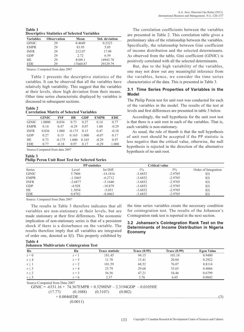
Table 1Descriptive Statistics of Selected Variables Variables Observation Mean Std. deviationGINIC 29 0.4649 0.2323EMPR 29 83.95 5.05INFR 29 212.07 17.99GDP 29 2.72 6.59HE 29 8109.1 14943.78EDE 29 17660.87 29129.79Source: Computed from data 2007

Table 1 presents the descriptive statistics of the variables. It can be observed that all the variables have relatively high variability. This suggest that the variables at their levels, show high deviation from their means. Other time series characteristic displayed by variables is discussed in subsequent sections.

Table 2Correlation Matrix of Selected Variables

GINIC INF HE GDP EMPR EDEGINIC 1.0000 0.036 0.73 0.27 0.14 0.77EMPR 0.14 0.47 -0.29 0.07 1.00 -0.29INFR 0.036 1.000 -0.175 0.15 0.47 -0.18GDP 0.27 0.15 0.165 1.000 -0.07 0.17HE 0.73 -0.175 1.000 0.165 -0.29 0.97EDE 0.77 -0.18 0.97 0.17 -0.29 1.000Source:Computed from data 2007

The correlation coefficients between the variables are presented in Table 2. This correlation table gives a preliminary idea of the relationship between the variables. Specifically, the relationship between Gini coefficient of income distribution and the selected determinants. As observed from the table, Gini coefficient (GINIC) is positively correlated with all the selected determinants.

But, due to the high variability of the variables, one may not draw out any meaningful inference from the variables, hence, we consider the time series characteristics of the data. This is presented in Table 3.

3.1 Time Series Properties of Variables in the ModelThe Philip Peron test for unit root was conducted for each of the variables in the model. The results of the test at levels and first differences are presented in table 3 below.

Table 3Philip Peron Unit Root Test for Selected Series

PP statistics Critical valueSeries Level Ist Diff. 1% 5% Order of IntegrationGINIC 5.7806 -14.1816 -3.6852 -2.9705 I(l)EMPR -1.5465 -6.2712 -3.6852 -2.9705 I(l)INFR -2.6877 -5.1640 -3.6852 -2.9705 I(l)GDP -4.928 -10.879 -3.6852 -2.9705 I(l)HE 1.3854 -5.051 -3.6852 -2.9705 I(l)EDE 0.8782 -8.0463 -3.6852 -2.9705 I(l)Source: Computed from Data 2007

Accordingly, the null hypothesis for the unit root test is that there is a unit root in each of the variables. That is, each variable is non-stationary.

As usual, the rule of thumb is that the null hypothesis of unit root should be accepted if the PP statistic is less negative than the critical value, otherwise, the null hypothesis is rejected in the direction of the alternative hypothesis of no unit root.

The results in Table 3 therefore indicates that all variables are non-stationary at their levels, but are made stationary at their first differences. The economic implication of non-stationary series is that of a persistent shock if there is a disturbance on the variable. The results therefore imply that all variables are integrated of order one, denoted as I(l). This property exhibited by

the time series variables create the necessary condition for cointegration test. The results of the Johansen’s Cointegration rank test is reported in the next section.

3.2 Johansen’s Cointegration Rank Test on the Determinants of Income Distribution in Nigeria Economy

Table 4Johansen Multivariate Cointegraton TestHo Ha Trace statistic Trace (0.95) Trace (0.99) Egen Valuer = 0 r = 1 181.45 94.15 103.18 0.9480r < 4 r = 5 11.70 15.41 20.04 0.2922r < 1 r = 2 101.59 68.52 76.07 0.8114r < 3 r = 4 25.79 29.68 35.65 0.4066r < 2 r = 3 56.56 47.21 54.46 0.6799r < 5 r = 6 2.37 3.76 6.65 0.0842Source:Computed from Data 2007

GINIC = -6331.16 + 74.367EMPR + 0.3298INF – 2.3194GDP – 0.0105HE (17.77) (0.1088) (0.3107) (0.002) + 0.0046EDE ��(3) (0.0011)



The Likelihood Ratio (LR) test based on the trace statistic is reported in Table 4. The null hypothesis of no cointegration is rejected up to r < 2, implying that there are at least 3 cointegrating equations at 1% and 5% significance level, among the I(1) variables. This is so because at r < 0, r < 1 and r < 2 the trace statistics are greater than the critical values respectively at 1% and 5% levels.

The evidence of cointegration indicates that, inflation rate, employment rate, growth rate of output, health and education expenditure are long-run determinants of income distribution. The long-run relationship was represented in equation (3). It is observed from the equation that employment rate, inflation rate and education expenditure all show positive relationship to the Gini coefficient, while, growth rate of output and health expenditure show negative relationship.

Note, that GINI coefficient is a measure of the rate of inequality of income distribution in an economy. The higher the coefficient the higher the inequality of income distribution. As discussed under the trend of income distribution in Nigeria, the coefficient has been on the increase in Nigeria, tending towards extreme inequality (above 0.75). The relationship in equation (3) is justifiable, the rate of employment in Nigeria has not been sufficient to reduce inequality of income distribution, else, it widens the gap. A unit of employment created increases inequality with about 74 percent. In most cases, employment generated are mainly to sustain living and not for wealth creation, thus, instead of redistributing income, it further creates low-level income earners.

Also, inflation rate increases the gap between the rich and the poor. A unit increase in inflation rate widens the inequality gap with about 0.33 percent. This is so because, inflation rate reduces the purchasing power of income, and this mostly affects the low-income earners. The rate at which education expenditure affects GINI coefficient in the long-run is low and more or less insignificant.

Growth of output (GDP) was found to reduce inequality in the longrun as shown in equation (3). The precise shape of inequality-growth relationship is not totally depicted by equation (3) as the relationship could be more than unidirectional.

We have first established that income distribution and its determinants are cointegrated; that is, a long term or equilibrium relationship existed among the variables. In the short run, there may be disequilibrium. The error term in equation (3) is treated as the disequilibrium error, the sign and magnitude of which links the short-run and long-run relationship. The results of the Error-Correction Mechanism (ECM) is reported in the next section.

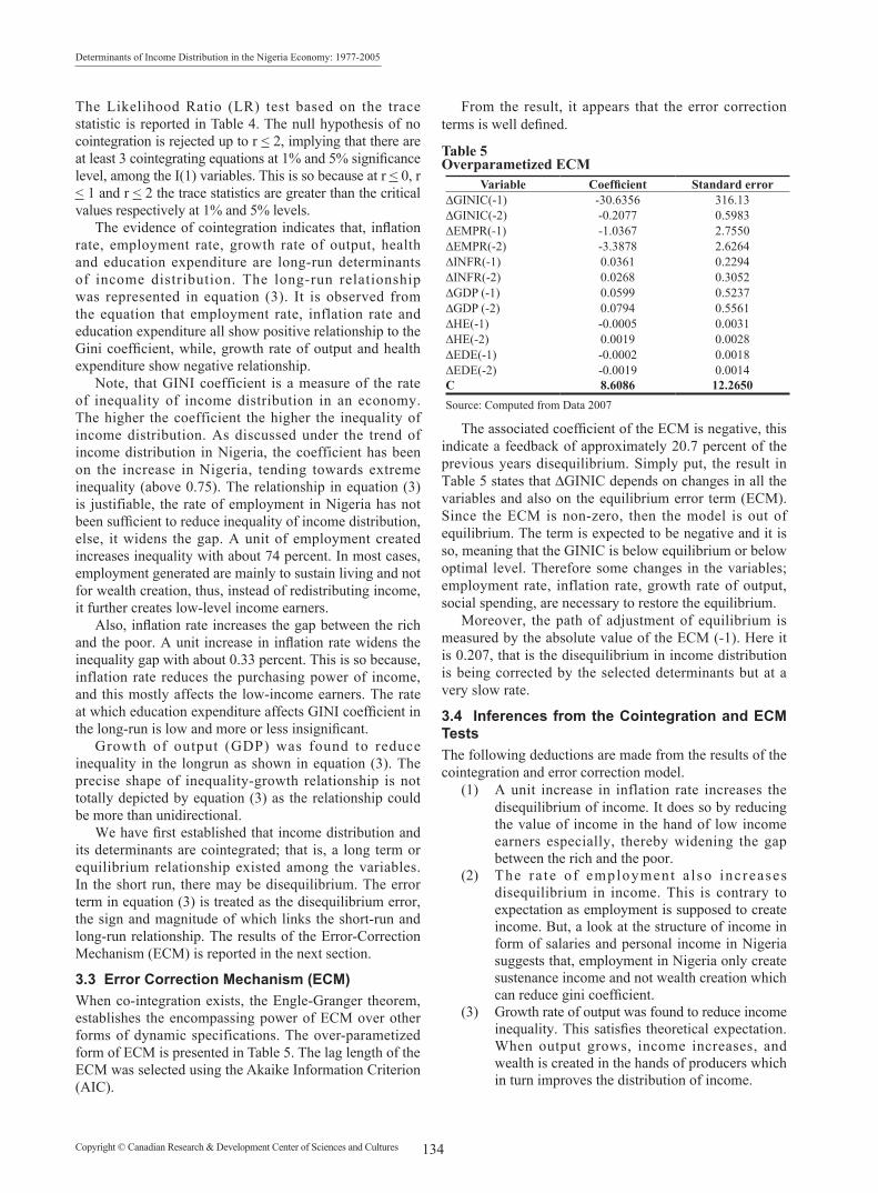
3.3 Error Correction Mechanism (ECM)When co-integration exists, the Engle-Granger theorem, establishes the encompassing power of ECM over other forms of dynamic specifications. The over-parametized form of ECM is presented in Table 5. The lag length of the ECM was selected using the Akaike Information Criterion (AIC).

From the result, it appears that the error correction terms is well defined.

Table 5Overparametized ECM

Variable Coefficient Standard error∆GINIC(-1) -30.6356 316.13∆GINIC(-2) -0.2077 0.5983∆EMPR(-1) -1.0367 2.7550∆EMPR(-2) -3.3878 2.6264∆INFR(-1) 0.0361 0.2294∆INFR(-2) 0.0268 0.3052∆GDP (-1) 0.0599 0.5237∆GDP (-2) 0.0794 0.5561∆HE(-1) -0.0005 0.0031∆HE(-2) 0.0019 0.0028∆EDE(-1) -0.0002 0.0018∆EDE(-2) -0.0019 0.0014C 8.6086 12.2650Source: Computed from Data 2007

The associated coefficient of the ECM is negative, this indicate a feedback of approximately 20.7 percent of the previous years disequilibrium. Simply put, the result in Table 5 states that ∆GINIC depends on changes in all the variables and also on the equilibrium error term (ECM). Since the ECM is non-zero, then the model is out of equilibrium. The term is expected to be negative and it is so, meaning that the GINIC is below equilibrium or below optimal level. Therefore some changes in the variables; employment rate, inflation rate, growth rate of output, social spending, are necessary to restore the equilibrium.

Moreover, the path of adjustment of equilibrium is measured by the absolute value of the ECM (-1). Here it is 0.207, that is the disequilibrium in income distribution is being corrected by the selected determinants but at a very slow rate.

3.4 Inferences from the Cointegration and ECM Tests The following deductions are made from the results of the cointegration and error correction model.

(1) A unit increase in inflation rate increases the disequilibrium of income. It does so by reducing the value of income in the hand of low income earners especially, thereby widening the gap between the rich and the poor.

(2) The ra te of employment a l so increases disequilibrium in income. This is contrary to expectation as employment is supposed to create income. But, a look at the structure of income in form of salaries and personal income in Nigeria suggests that, employment in Nigeria only create sustenance income and not wealth creation which can reduce gini coefficient.

(3) Growth rate of output was found to reduce income inequality. This satisfies theoretical expectation. When output grows, income increases, and wealth is created in the hands of producers which in turn improves the distribution of income.



(4) Social spending shows a dual relationship with income distribution. While education expenditure was found to have widen the inequali ty gap, health expenditure closes the gap. The relationship of government education expenditure to income distribution observed here support the argument of Anand (1983), that if human capital is not well distributed or insufficient, it brings about inequality in income rather than welfare. For some times now, the education sector in Nigeria have been under-funded thereby making the sector less effective in solving the problem of inequality in income distribution.

(5) Improvement s in a l l t he de te rminan t s , according to ECM results, was found to have been correcting the disequilibrium in income distribution but at a very slow rate.

CONCLUSION Sequel to the results and the findings in this study, the following logical, coherent and sequential conclusions are made:

(1) There is a longrun positive relationship between employment rate and Gini Coefficient of income distribution in Nigeria. That is, employment rate increases income inequality in Nigeria.

(2) There is a longrun positive relationship between inflation rate and Gini Coefficient of income distribution in Nigeria, since, inflation rate widens the gap between the rich and the poor. Also inflation rate reduces the purchasing power of income of the junior workers thereby widening income gap in Nigeria.

(3) There is longrun, inverse relationship between output growth and Gini Coefficient of income distribution in Nigeria. Growth rate of output (GDP) increases income and wealth is created in the economy which increases the distribution of income in Nigeria.

(4) Also, there is a longrun positive relationship between government education expenditure and Gini Coefficient of income distribution in Nigeria i.e. expenditure on education rather than reducing income inequality, widens it in Nigeria while government health expenditure exhibited and inverse relationship with Gini coefficient of income distribution i.e. health expenditure closes income gap in Nigeria but at a very slow rate.

(5) The study also concluded that, employment rate, inflation rate, Gross Domestic Product and social spending are true determinants of income distribution in Nigeria.

(6) A negative coefficient of the overparametized ECM which shows that changes in the Gini coefficient of income distribution depends on changes in all the variables and also on the equilibrium error term (ECM), further justifies the existence of long run relationship between income distribution and its determinants.

POLICY RECOMMENDATIONS From the empirical findings in this research work and based on the relationship each determinant of income exhibited with the Gini coefficient of income distribution in Nigeria economy, the following recommendations are made to enhance a more evenly distribution of income which would in effect, reduce income gap and poverty in Nigeria.

(1) Efforts of the government should be mobilized towards the formulation and implementation of more pragmatic employment policies in Nigeria. Since the empirical findings in this research work have shown that a rise in employment rate has not been sufficient to reduce inequality of income distribution in Nigeria. A more pragmatic employment policy would enable workers to create wealth from their income (and not just for sustenance) which enhances a more evenly distribution of income.

(2) If the efforts of Nigerian government on wage increase is going to yield more positive result then, a policy to reduce the current inflation rate of 2-digits to 1-digit must be priotised. A considerable rate of inflation would help increase the real value of income in the hand of workers especially the low income earners thereby closing the gap between the rich and the poor. Our findings in this empirical work indicated that a rise in inflation rate widens income gap in Nigeria, therefore, simultaneous policies for wage increase and that which controls the growth rate of inflation should be given more priority in Nigeria.

(3) Also, empirical findings from this research work indicated that, output growth reduces inequality of income distribution. Odedokun and Jeffery (2001) found that increase in output would reduce inequality of income in the economy. Therefore, effort of the government should be geared towards the improvement of national output (GDP) in the Nigerian economy.

(4) Government should a l so ensure p roper monitoring of its spending on education and health, through appropriate policy measures. This will checkmate the diversion of funds meant to boost educational growth and health care delivery in Nigeria. Todaro (2000) stated that the lack of prudence in LDC’s public expenditure management has contributed immensely to the wide gap between the rich and the poor. The empirical findings in this research work indicated that, a rise in education expenditure rather than reducing inequality of income distribution, widens it. This implies that expenditure on education does not commensurate with the output realized. Hence, policies that would enhance proper monitoring of these processes should be formulated and implemented by Nigerian government. Also, the empirical findings from the study revealed that a rise in health expenditure



reduces gini coefficient of income distribution in Nigeria. Therefore, government should intensify efforts in ensuring proper monitoring of funds allocated to the health sector, so as to boost health care delivery in the country.

(5) Finally, a set of policies designed to bring about a more equitable distribution of income, equal access to education and associated income earning opportunities should be given priority in Nigeria. Such policies should be targeted towards ensuring that the income gap between the rich individuals and the poor individual in Nigeria is further closed.

REFERENCESAboyade, O. (1974). Income Structure and Economic Society,

Nigeria Economic Society (NES) Conference in: (NES), The Construction Industry in Nigeria. Ibadan, University Press.

Aboyade, O. (1978). Integrated Economics: A Case Study of Developing Economies. English Language Book Society.

Adams, R.H. (Jr) (1999). Nonfarm Income, Inequality and Land in Rural Egypt PRMPO/MNSED, Washington. Unpublished Report for Comment, World Bank.

Adams, R.H. (Jr), & HE, J.J. (1995). Sources of Income Inequality and Poverty in Rural Pakistan (Research Report, 102). International Food Policy Research Institute. Washington.

Alayande , B . (2003) . Decompos i t ion o f Inequa l i ty Reconsidered: Some Evidence from Nigeria. Paper Presented at the UNU/WIDER Conference on Inequality, Poverty and Human well being in Helsinki, Finland between 29th and 31st of May, 2003.

Awoyemi, B.T. (2005). Explaining Income Inequality in Nigeria: A Regression Based Approach. Journal of Economics and Rural Development, 4(6), 45-59.

Bouillon, C.P., Legovini, A., & Lustig, N. (2001). Rising Inequality in Mexico: Household Characteristic and Regional Effects. JEL Classification D1. Part of Research Report on “The Microeconomic of Income Distribution Dynamics in East Asia and Latin America”.

Bulir, A. (1998). Income Inequality “Does Inflation Matter?” IMF Working Paper, 98/7, 48(1). Washington, International Monetary Fund.

Canagarajah, S., Ngwafon, J., & Thomas, S. (1997). The Evolution of Poverty and Welfare in Nigeria, 1985-92. Policy Research Working Paper No. 1715.

Cornia, G.A. (2004). Changes in the Distribution of Income over the Last Two Decades, Extents, Sources and Possible Causes. Rivista Italiana Degli Economisti, 9(3), 69-84.

Deininger, K., & Squire L. (1996). Measuring Income Inequality: A New Data-Base. Development Discussion Paper No. 537. Cambridge, Massachusetts: Harvard Institute for International Development.

Deijomaoh, V.P., & Ansionwu, S. (1985). Income Distribution and Poverty Growth in Developing Economies. NBER working papers, 4798.

Elbers, C., Lanjouw, P., Mistiaem, J., Ozler, B., & Similar, K. (2003). Are Neighbours Equal? Estimating Local Inequality in Three Developing Countries. WIDER Discussion Paper No. 2003/52.

Fajana, C.O. (1985). The Empirical Analysis of the Relationship Between Differential in Earnings of Employed and Employee Power in Some Selected Manufacturing Firms in Nigeria. Journal of Development Economics, 38, 23-32.

Granger, C.W.J. (1969). Investigating Causal Relations by Econometric Models and Cross-Spectral Methods. Econometrica, 37, 169-187.

Gujarati, D.N. (2007). Basic Econometrics (4th ed.). New York: Mc-Graw Hill.

Jacobs, D. (2000). Low Inequality with Low Redistribution? An Analysis of Income Distribution in Japan, South Korea and Taiwan Compared to Britain. CASE Paper 33 Centre for Analysis of Social Exclusion. London School of Economics Houghton Street London.

Jones, R. (2007). Income Inequality, Poverty and Social Spending in Japan. European Journal of Polical Economy, 18(4). Retrieved 20 Feb, 2007, from http://www.olisoecd org/olis doc-list 43 bb 61 30e5eb.

Jose, D., & Teilings, G. (2002). Determinants of Income Distribution. New Evidence from Cross Country Data, Korea University.

Kuznet, S. (1963). Quantitative Aspect of the Economic Growth of Nations: Distribution of Income by Size. Economic Development and Cultural Change, 2, 51-80.

Kuznet, S. (1955). Economic Growth and Income Inequality. American Economic Review, 45, 1-28.

Morduch, J., & Sicular, T. (2002). Rethinking Inequality Decomposition with Evidence from Rural China. The Economic Journal, 112, 93-106.

Nnanna, O. J., Alade, S.O., & Odoko, F.O. (2003). Contemporary Economic Policy Issues. Cental Bank Nigeria Publications.

Odedokun, M.O., & Jeffery, I. (2001). Determinants of Income Inequality and Its Effects on Economic Growth: Evidence from African Countries. Journal of Economic Literature, 39(4). Retrieved on 16 Feb, from http://www.wider.unu.edu/stc/repec/pdfs/2001/dp2001-103.PDF.

Oguntuase, A. (2007). An Empirical Investigation into the Determinants of Income Distribution in the Nigerian Manufacturing Sector (Unpublished M.Sc Thesis). Ekiti State University.

Ogwumike, F.O., Alaba, O.B., Alaba, Alayande, B.A., & Okojie, B.A., C. E. E. (2003). Labour Force Participation, Earnings and Income Inequality in Nigeria. A World Bank Report.

Oyekale, A.S. (2005). Sources of Isncome Inequality and Poverty in Rural and Urban Nigeria. Journal of Development Economics, 51, 267-290.

Piesse, Simister J.J., & Thirtle, S. (1998). Modernization, M u l t i p l e I n c o m e S o u r c e s a n d E q u i t y : A G i n i Decomposition for the Communal Lands in Zimbabwe, JEZ Classification: D31.

Rossana, G., & Hoeven, R.V.D. (2001). Is Inflation Bad for Income Inequality? The Importance of Initial Rate of Inflation.



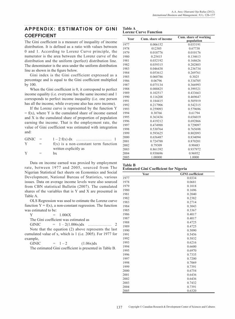
APPENDIX: ESTIMATION OF GINI COEFFICIENTThe Gini coefficient is a measure of inequality of income distribution. It is defined as a ratio with values between 0 and 1. According to Lorenz Curve principle, the numerator is the area between the Lorenz curve of the distribution and the uniform (perfect) distribution line. The denominator is the area under the uniform distribution line as shown in the figure below.

Gini index is the Gini coefficient expressed as a percentage and is equal to the Gini coefficient multiplied by 100.

When the Gini coefficient is 0, it correspond to perfect income equality (i.e. everyone has the same income) and 1 corresponds to perfect income inequality (i.e. one person has all the income, while everyone also has zero income).

If the Lorenz curve is represented by the function Y = f(x), where Y is the cumulated share of income earned and X is the cumulated share of proportion of population earning the income. That is the employment rate, the value of Gini coefficient was estimated with integration and:

GINIC = 1 – 2 f(x) dx �� 1Y = f(x) is a non-constant term function

written explicitly as Y = bx

Data on income earned was proxied by employment rate, between 1977 and 2005, sourced from The Nigerian Statistical fact sheets on Economics and Social Development, National Bureau of Statistics, various issues. Data on average income levels were also sourced from CBN statistical Bulletin (2007). The cumulated shares of the variables that is Y and X are presented in Table A.

OLS Regression was used to estimate the Lorenz curve function Y = f(x), a non-constant regression. The function was estimated to be:

Y = 1.006XThe Gini coefficient was estimated as GINIC = 1 – 2(1.006x)dx �� 2Note that the equation (2) above represents the last

cumulated value of x, which is 1 (i.e. 2005). For 1977 for example,

GINIC = 1 – 2 (1.06x)dxThe estimated Gini coefficient is presented in Table B.

Table ALorenz Curve Function

Year Cum. share of income Cum. share of working population

1977 0.006152 0.0331911978 012305 0.677381979 0.018776 0.0101761980 0.25415 0.1346131981 0.032192 0.1686261982 0.039315 0.2028031983 0.046438 0.2367341984 0.053612 0.2697611985 0.060786 0.30251986 0.06796 0.3347051987 0.075134 0.3669931988 0.088825 0.3993211989 0.102517 0.4336631990 0.116208 0.4696471991 0.184415 0.5059191992 0.217906 0.5423151993 0.259093 0.5796961994 0.30766 0.617941995 0.363436 0.6560191996 0.419212 0.6928661997 0.474988 0.7290971998 0.530764 0.7656981999 0.593625 0.8020932000 0.656487 0.8340942001 0.724788 0.8702012002 0.79309 0.904832003 0.861392 0.9379722004 0.930696 0.969522005 1.00000 1.0000

Table BEstimated Gini Coefficient for Nigeria

Year GINI coefficient 1977 0.03341978 0.06811979 0.10181980 0.16961981 0.20401982 0.23821983 0.27141984 0.30431985 0.33671986 0.40171987 0.40171988 0.47251989 0.47251990 0.50901991 0.54561992 0.58321993 0.62161994 0.66001995 0.69701996 0.73351997 0.72001998 0.70691999 0.73912000 0.67542001 0.64362002 0.64362003 0.74322004 0.73912005 0.6320

determinants of income distribution in the nigeria economy

Documents