air pollution and per capita income - political economy research

POLITIC

AL EC

ON

OM

YR

ESEAR

CH

INSTITU

TE

Gordon Hall

Amherst, MA, 01002-1735Telephone: (413) 545-6355Facsimile: (413) 577-0261 Email:[email protected]

Website: http://www.umass.edu/peri/

Deepening Divides in Jobless Recovery

Robert Pollin

2004

Number 82

POLITICAL ECONOMY RESEARCH INSTITUTE

University of Massachusetts Amherst

WORKINGPAPER SERIES

418 N. Pleasant St, Suite A

Air Pollution and Per Capita Income

Rachel A. Bouvier

2004

Number 84

AIR POLLUTION AND PER CAPITA INCOME: A Disaggregation of the Effects of Scale, Sectoral Composition,

and Technological Change

Rachel A. Bouvier

Department of Economics

Wellesley College

June 2004 Abstract During the last decade, researchers have investigated the relationship between per capita income and environmental quality. This paper disaggregates the relationship between per capita income and emissions of carbon monoxide, carbon dioxide, sulfur dioxide, and volatile organic compounds into scale, composition and technology effects, using data from European and North American countries from the period 1980-1986. Results indicate that the scale effect outweighs the composition and technology effects in the cases of carbon dioxide and volatile organic compounds, while the opposite is true in the cases of carbon monoxide and sulfur dioxide. The results also suggest that greater democracy is associated with lower emissions of all four pollutants. Key words: Environmental Kuznets curve; emissions; carbon monoxide; carbon dioxide; sulfur dioxide; volatile organic compounds.

1

1. Introduction In 1992, researchers at the World Bank profiled how six environmental problems, ranging from carbon dioxide emissions to the percentage of the population without access to safe drinking water, respond to changes in per capita income. They described three distinct patterns: some environmental problems worsened as per capita income increased (municipal wastes per capita and carbon dioxide emissions per capita); some improved along with per capita income (the percentage of the population without safe water or adequate sanitation, and concentrations of airborne particulate matter); and some initially worsened and then eventually began to improve (concentrations of sulfur dioxide) (World Bank, 1992:11). Curiously, it is the latter which has most captured the attention of many economists and policy makers. The “inverted U” described by the trajectory of sulfur dioxide concentrations against per capita income – called the “environmental Kuznets curve” due to its similarity to the theoretical relationship between per capita income and inequality first suggested by Kuznets (1955) – has been used incautiously by some to conclude that “in the end the best – and probably the only – way to attain a decent environment … is to become rich” (Beckerman, 1992). Tempting as it may be to arrive at this conclusion, it would be unwise for several reasons. First, as the World Bank found, the phenomena that fall into the “inverted-U” category represent only a subset of environmental problems. Second, as Arrow et al. (1995:520) point out, the inverted U does not “constitute evidence that it [the decline of pollution] will…happen in time to avert the important and irreversible global consequences of growth.” Third, as Grossman and Krueger (1995) state, there is nothing automatic about relationships that have proven true – in some places – in the past. While pollution levels may have declined after some turning point in some developed countries as per capita income grew, this does not necessarily imply that the same can or will occur in developing countries. For this reason, one must consider the underlying reasons behind such a curve, where it exists. The empirical literature on the environmental Kuznets curve typically is based on reduced-form equations that estimate the net effect of per capita income on pollution. Grossman and Krueger distinguish three effects that mediate this relationship, but they do not attempt to disentangle them empirically. This paper is an effort to do so, first by separating out the scale effect and then by investigating the impacts of variables related to the composition and technology effects. The next section describes each of these effects in turn. Section 3 then presents the econometric model to be used. Section 4 discusses the data, Section 5 summarizes the results, and Section 6 concludes.

2

2. The Scale, Composition, and Technology Effects The scale effect arises from the simple fact that economies with higher per capita incomes both produce and consume more goods and services. Holding output mix and production techniques constant, an increase in scale necessarily brings about a proportionate increase in pollution. Generally, however, as per capita income grows, both the output mix and production techniques change. Depending on the direction of these changes, a given unit of income may be associated with less or more pollution. If the scale effect is outweighed by pollution-reducing composition and/or technology effects, total pollution will fall with rising income. The scale effect can be expected to track year-to-year changes in the level of output and income, rising and falling with business cycle fluctuations, but the latter effects can be expected to operate more gradually. In the industrialized countries, economic growth has been accompanied by a shift in consumption patterns from the more material- and energy-intensive manufacturing sector toward the (theoretically) more environmentally-friendly service sector (Jayadevappa and Chhatre, 2000: 178). In addition, international trade permits a country’s production patterns to diverge from its consumption patterns, as its citizens consume goods produced in other countries and produce goods consumed elsewhere. Both can contribute to the “composition effect” of rising per capita incomes. The technology effect allows for the possibility that as countries develop, “cleaner” technologies substitute for “dirtier” ones in the production of any given commodity. As a result, pollution per unit of output could decline while holding the output mix constant. If the technology effect were sufficiently strong, total pollution could decline even as output rises. The technology effect can be separated into two elements. One is the “autonomous” technology effect, in which the substitution of cleaner processes occurs more or less automatically for exogenous reasons. The other is the “induced” technology response, whereby demand for a cleaner environment is translated into public and private decisions to cut pollution.1 Technological change in response to regulatory mandates, such as compulsory installation of end-of-pipe scrubbers in stacks to reduce sulfur dioxide emissions, is an example. The possibility of such induced technology responses suggests that an important intervening variable in the income-pollution relation may be the extent of democracy, such that demand for environmental quality is politically effective (see

1 This builds on Hicks’ (1939) distinction between technological change brought about by changes in the relative price of factors (induced technological change) versus exogenous growth in scientific and technical knowledge. For a comprehensive literature survey on induced versus autonomous technological change and environmental quality, see Jaffe et al. (1995).

3

Barrett and Graddy, 2000; Torras and Boyce, 1998). For this reason, the induced technology response is sometimes called the “political economy” effect (Heerink et al, 2001). To advance our understanding of the relationship between environmental degradation and per capita income, it would be useful to be able to distinguish empirically among the scale, composition, and technology effects, and to assess their relative strength. Stern (2002) attempts to measure the composition effect by including variables measuring the value-added shares of agriculture, manufacturing, and other sectors as determinants of pollution; to proxy the technology effect he uses total energy inputs. Once these are included, he treats the estimated coefficient on per capita income as a measure of the scale effect. Baldson (2003) interacts measures of the degree of democracy with per capita income to assess the technology effect, reasoning that “‘abatement’ (technique) effects are fundamentally interacted with government in a way that ‘gross emissions’ (or scale) are not, leading to an econometric specification capable of identifying them separately.” However, he makes no attempt to identify the composition effect. In this paper, I propose an alternative methodology for disaggregating the three effects.

3. A Disaggregated Model of the Income-Degradation Relationship

3.1 Trend versus fluctuations

I begin by estimating separately the environmental impact of the trend in GDP and that of fluctuations around that trend. The composition and technology effects are assumed to operate only through the trend: they are expected to affect the income-degradation relation gradually, with little sensitivity to year-to-year income fluctuations. The scale effect, on the other hand, is apparent in the effects of the year-to-year fluctuations in income around that trend. These short-run variations in GDP, unlike long-run growth, are not expected to alter substantially the composition of output or technology. Figure 1 depicts the per capita income in a hypothetical country where it trends upward in a linear fashion. The curved line indicates the observed level of per capita GDP; the dashed line indicates the level predicted by the time trend. Previous econometric models of the relationship between per capita income and emissions have used (Yit), the observed income in country i at time t, as the independent variable. Decomposing this into fluctuations and trend, we can obtain two independent variables: Yit*, the trend level of income, and (Yit – Yit*), the fluctuations around that trend. The impact of income fluctuations on environmental degradation can be attributed to the scale effect, while the impact of the income trend is attributable not only to the changes in the scale but also to composition and technology effects.

Yt trend of GDP over time Y*t Y t time

Figure 1: Trend versus fluctuation of income

3.2 Model

The full econometric model estimated in this paper is: lnPolit = α + β1lnYit* + β2(lnYit*)2 + β3ln(Yit - Yit*) + β4(Popit/km2) +β5(Popit/km2)2 + + β6(Iit/Sit)+ β7DEMOCit + βiIDi +µit (1) where: Polit = the per capita emissions level; Yit*= the trend value of income; 2 Yit = the actual value of per capita GDP; Popit/km2= population per kilometer squared; Iit = the percentage of GDP that comes from value added in the industrial Sit = the percentage of GDP that comes from value added in the service sector DEMOCit is an index of democracy IDi = country-specific dummy variables; µit is the error term, whose properties will be discussed below; and the subscripts i and t refer to the country and year, respectively. Equation (1) implies that the pollution level can be explained by the income trend, income fluctuations, sectoral composition of output (Iit/Sit), and the democracy index,

2 The income trend variable is obtained by regressing the log of per capita GDP on the year and year squared, and obtaining the fitted values. The income fluctuations are the residuals of this equation.

5

with population density included as a control variable.3 The equation will be estimated by feasible generalized least squares. The scale effect is estimated as a constant elasticity by the coefficient β3. The elasticity of emissions with respect to the trend level of income is estimated by the following equation: εey = β1 + 2(β2)[mean (lnY)] (2) The trend elasticity captures the scale, composition and technology effects combined. Hence, (εey - β3) gives an estimate of the effects of composition and technology. The sectoral composition variable is added in an effort to isolate the composition effect; insofar as it does so, (εey - β3) provides an estimate of the technology effect alone. The democracy variable is added in an effort to further separate out the induced “political economy” component of the technology effect. Insofar as it does so, the value of (εey - β3) provides an estimate of the autonomous component of the technology effect alone. The strength of the induced technology effect may differ by pollutant: it can be expected to be stronger for pollutants that have greater visibility – literally and metaphorically – and hence are more subject to public demand for emissions reductions. This study investigates four different pollutants: carbon dioxide, carbon monoxide, sulfur dioxide, and volatile organic compounds. The characteristics of each are discussed in the next sub-section.

3.3 Discussion of pollutants studied

The pollutants investigated in this study – carbon monoxide, carbon dioxide, sulfur dioxide, and volatile organic compounds – were chosen because of their contrasting characteristics, as well as the fact that data on emissions are available for a large number of industrialized countries. Pollution is measured in metric tons of emissions per capita. Some studies of the income-degradation relationship have used ambient concentrations, rather than emissions, as the dependant variable. Both measures have advantages and drawbacks. If the goal is to study how environmental quality changes with economic growth, then ambient concentrations are a preferable measure for localized pollutants. However, ambient concentrations are affected by geographical variables such as topography, climate, and wind. For example, the existence of hills or thermal inversions may limit dispersion of contaminants. The fact that ambient concentrations vary from place to place within any given country makes determining the appropriate measure for

3 Population density has been used in other studies of air pollution (see, for example, Selden and Song, 1994), as sparsely populated countries may be less likely to consider lowering per capita emissions as a priority.

6

national-level analysis problematic.4 Moreover, for globalized pollutants such as CO2, the level of emissions is the only appropriate measure.

3.3.1 Carbon monoxide

Carbon monoxide (CO) is a colorless, odorless gas, arising from the incomplete burning of fossil fuels (OSHA, 2002). In the United States, emissions of carbon monoxide generally decreased from 1970 to 1995, but then increased again (World Almanac Book of Facts, 2003:166). The atmospheric concentration of carbon monoxide in the U.S. nonetheless continued to decline, possibly because increased ultraviolet radiation, due to the thinning of the ozone layer, creates hydroxyl radicals that react rapidly with carbon monoxide (Khalil, 1995: 7). Although carbon dioxide and carbon monoxide both arise from the combustion of fossil fuels, the contaminants exhibit different fates. Carbon dioxide persists in the atmosphere, whereas carbon monoxide remains in the atmosphere for an average of two months. Therefore, changes in emissions of carbon monoxide have a more rapid effect on atmospheric concentrations. Although carbon monoxide is odorless and colorless, its localized health effects (shortness of breath and dizziness, for example) make it a good candidate for a strong political economy effect. In the U.S., for example, CO is among the “criteria air pollutants” regulated under the Clean Air Act of 1970.

3.3.2 Carbon dioxide

Carbon dioxide (CO2), like its cousin, is a colorless, odorless gas, released from fossil fuel combustion. As one of the primary culprits in global warming, CO2 is a pure “public bad” whose effects are not restricted by country boundaries. As such, it is subject to the international “free rider” problem: individual countries may not be willing to enforce controls on carbon dioxide emissions, as they would receive only a small fraction of the benefits while bearing the full costs. Therefore, the political economy effect may not be as strong for carbon dioxide as for some other more visible and localized contaminants. In the U.S., for example, the Environmental Protection Act does not attempt to regulate CO2 emissions.5 However, concern about global warming has been growing in the past decade or so. In the 2002 “Eurobarometer” (an extensive survey of the attitudes of Europeans towards their environment), 39% of those surveyed reported that they were “very worried” about climate change (EORG, 2002: 8). With the signing of the Kyoto Protocol, and subsequent discussions of “carbon taxes” in Europe, public awareness of carbon dioxide emissions is on an upswing in many countries.

4 In addition, there is the issue of the spatial separation between emissions and concentrations: “Using emissions neither ‘punishes’ countries that import pollution from areas over which they have little political control nor ‘rewards’ those that export pollution via prevailing winds” (Scruggs, 1998: 296). 5 In fact, under the current administration, the U.S. EPA heavily edited a report on the state of the environment to include only cursory mention of global warming and climate change (Herbert, 2003).

7

3.3.3 Sulfur dioxide Sulfur dioxide is a colorless gas with a pungent odor. It is formed when fuels containing sulfur (mainly coal and oil) are burned, and during various industrial processes, such as smelting. Short-term exposure to high levels of sulfur dioxide can be life-threatening. Long-term exposure to atmospheric sulfur dioxide can lead to or exacerbate asthma and other respiratory illnesses, and aggravate existing heart disease (U.S. Environmental Protection Agency, 2003). In addition, sulfur dioxide is a precursor to acid rain, which leads to the corrosion of buildings, monuments, and other structures, and has adverse impacts on forests and aquatic ecosystems. Sulfur dioxide in the atmosphere is highly visible (politically speaking) and thus is a prime candidate for an induced policy response. However, public interest and concern about acid rain has been declining over the last decade, in both the United States (Gallup et al., 2000) and Europe (EORG, 2002: 8). In addition, because SO2 can be transported long distances, there is potential for transboundary separation between the point of origin and the point of impact, diminishing the likelihood of an effective political economy effect.

3.3.4 Volatile organic compounds

Volatile organic compounds (VOCs), a class of volatile (easily evaporating) carbon-containing compounds such as carbon tetrachloride, trichloroethene (TCE) and benzene, are found in many solvents and paints used in industrial activities and many household items. Unless disposed of properly, VOCs can enter the air, soil, and water, where they can remain for years (Brookhaven National Laboratories, 2002). The dispersion of sources of VOCs, compared to those of sulfur dioxide, may make their emissions more difficult to control. In addition, VOCs may be less visible in the public’s perception, possibly muting any political economy effect.

3.4 Hypotheses

Equation (1) will be estimated first without the sectoral composition and democracy variables. Income fluctuations are expected to have a positive coefficient, here interpreted as an estimate of the scale effect. If pollution exhibited constant returns to scale, the elasticity of emissions with respect to income fluctuations would be 1.0. It is possible, however, that emissions have both a fixed component that is more or less inelastic with respect to income fluctuations, as well as a variable component with approximately unit elasticity. If so, the estimated elasticity (which can be read directly from the coefficient in this specification since both variables are in natural logarithms) would be between zero and one. The elasticity of emissions with respect to the trend level of income is expected to be negative (meaning that the income trend is favorable for environmental quality) if the composition and technology effects outweigh the scale effect, and positive if they do not.

8

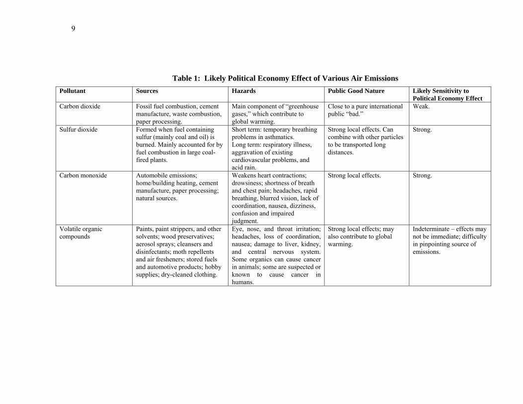
Next, the full model will be estimated in an effort to isolate some phenomena that contribute to the trend effect. The predicted sign on the sectoral composition variable is positive; that is, a higher ratio of industrial sector output to service sector output is expected to result in higher levels of emissions. The predicted sign on the democracy variable is negative; that is, countries with greater democracy (and a more equitable distribution of political power) are expected to have lower levels of emissions. The strength of this effect is expected to vary across pollutants, however, for the reasons discussed above. A typology of the pollutants and their likely political “responsiveness” (defined as how likely emissions are to elicit politically effective demand for pollution reduction) is presented in Table 1. The inclusion of the sectoral composition and democracy variables in the estimated equations is expected to reduce the difference between the elasticities of emissions with respect to the income trend and with respect to income fluctuations. Some difference is expected to remain, however, insofar as the trend effect also reflects autonomous technological change, and because the sectoral and democracy variables used here may be imperfect proxies for the composition and political economy effects.

3.5 Issues in Estimation

Equation (1) is estimated by a fixed-effects method. That is, each country is assumed to have its own intercept, while the slope coefficients are common to all countries. A log-ratio test was used to test for heteroskedasticity across panels: the model was estimated with and without correcting for panel-level heteroskedasticity, and their log ratios then compared. Evidence was found for panel-level heteroskedasticity; hence, the corrected results are reported here. First-order serial autocorrelation within panels can also be a problem. Durbin Watson tests were performed on the data for individual countries, and evidence of first-order serial autocorrelation was found in a number of cases. Hence, the feasible generalized least squares method was used to estimate the model.

9

Table 1: Likely Political Economy Effect of Various Air Emissions Pollutant Sources Hazards Public Good Nature Likely Sensitivity to

Political Economy Effect Carbon dioxide Fossil fuel combustion, cement

manufacture, waste combustion, paper processing.

Main component of “greenhouse gases,” which contribute to global warming.

Close to a pure international public “bad.”

Weak.

Sulfur dioxide Formed when fuel containing sulfur (mainly coal and oil) is burned. Mainly accounted for by fuel combustion in large coal-fired plants.

Short term: temporary breathing problems in asthmatics. Long term: respiratory illness, aggravation of existing cardiovascular problems, and acid rain.

Strong local effects. Can combine with other particles to be transported long distances.

Strong.

Carbon monoxide Automobile emissions; home/building heating, cement manufacture, paper processing; natural sources.

Weakens heart contractions; drowsiness; shortness of breath and chest pain; headaches, rapid breathing, blurred vision, lack of coordination, nausea, dizziness, confusion and impaired judgment.

Strong local effects. Strong.

Volatile organic compounds

Paints, paint strippers, and other solvents; wood preservatives; aerosol sprays; cleansers and disinfectants; moth repellents and air fresheners; stored fuels and automotive products; hobby supplies; dry-cleaned clothing.

Eye, nose, and throat irritation; headaches, loss of coordination, nausea; damage to liver, kidney, and central nervous system. Some organics can cause cancer in animals; some are suspected or known to cause cancer in humans.

Strong local effects; may also contribute to global warming.

Indeterminate – effects may not be immediate; difficulty in pinpointing source of emissions.

10

4. Data

4.1 Pollution data

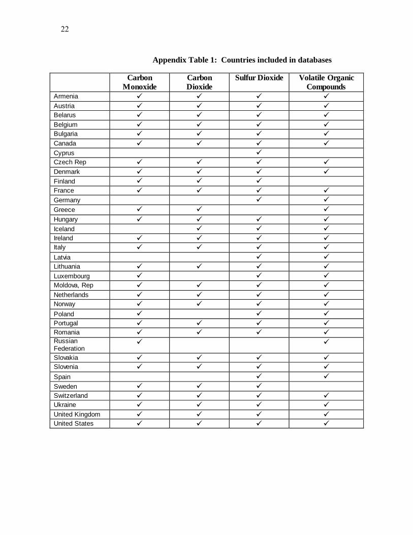
Pollution data for the years 1980 to 1996 were obtained from the World Resources Institute’s Earth Information Portal (2002).6 Emissions are divided by the population of the country to obtain per capita emissions. The available data include only European countries, Canada, and the United States – countries that reported their emissions to the Economic Commission for Europe whose per capita incomes (in 1987 PPP–adjusted dollars) range from $1100 to $24,371.7 Hence, one should be cautious about extrapolating the results to other countries. The country coverage varies by contaminant; Appendix Table 1 shows the countries covered by each database.

4.2 Economic and political variables

Data on the per capita level of GDP, adjusted for purchasing power parity, 8 also come from the World Resources Institute’s Earth Information Portal (2002), as do the democracy and population variables. The original data for the democracy index – a weighted measure of the competitiveness and openness of executive recruitment, the degree of limitations on the chief executive, and the competitiveness of political participation - are from the Polity IV project at the University of Maryland.9 The composition variable, which measures the value added in the industrial sector relative to that in the service sector, comes from the World Bank’s World Development Indicators, 1999. Summary statistics and correlation coefficients for all variables are reported in Tables 2 and 3, respectively.

6Carbon dioxide emissions figures come from the International Energy Agency, using the Reference Approach. This approach estimates the carbon content in primary fuels supplied to the economy. Apparent consumption of these fuels is derived by subtracting net exports from production, and accounting for net changes in stocks. “Double-counting” is avoided by not including the carbon contained in secondary fuels, but imports and exports of those fuels are included (see World Resources Institute, “Technical Notes”). 7 Data for carbon dioxide emissions are available for other countries, but for the sake of comparability, I analyze only those countries for which emissions data were found for at least one of the other contaminants. 8 The purchasing power parity adjustment ensures that countries with similar “real” income can purchase similar amounts and qualities of goods and services. 9 For detail, see (Marshall and Jaggers, 2002). The regime is coded for degree of democracy on a scale from 0 to 10, and for the degree of autocracy from 0 to 10. The variable used here is constructed by subtracting the autocracy score from the democracy score.

11

Table 2: Summary Statistics

Carbon Monoxide Sample Obs Mean Std. Dev. Min Max

CO (metric tons per 100 people) 325 14.65 8.75 2.25 52.29GDP (adjusted for PPP, hundreds of international 1987$ per person)

325 109.25 55.64 12.32 243.71

Industry / Service value added 272 0.76 0.47 0.25 2.30Democracy index 280 8.45 4.12 -8 10

Carbon Dioxide Sample Obs Mean Std. Dev. Min Max

CO2 (metric tons per 100 people) 368 887.6 372.7 73.9 2,097.3GDP (adjusted for PPP, hundreds of international 1987$ per person)

368 115.72 49.71 11.06 209.74


Sulfur Dioxide Sample Obs Mean Std. Dev. Min Max

SO2 (metric tons per 100 people) 434 0.598 0.453 0.008 2.70 GDP (adjusted for PPP, hundreds of international 1987$ per person)

434 106.83 53.40 12.32 243.71


Volatile Organic Compounds Sample Obs Mean Std. Dev. Min Max

VOC (metric tons per 100 people) 344 0.381 0.218 0.002 1.10 GDP (adjusted for PPP, hundreds of international 1987$ per person)

344 103.78 57.31 12.32 243.71


12

Table 3: Correlation Coefficients

Carbon Monoxide

Income Trend Income Fluctuations Ind/Serv Democracy

Income Trend 1 Income Fluctuations 1.61E-02 1 Industry/Service Value Added -0.724 7.33E-02 1 Democracy 0.516 -0.108 -0.739 1

Carbon Dioxide



Sulfur Dioxide



Volatile Organic Compounds


Income Trend 1 Income Fluctuations 4.40E-03 1 Industry/Service Value Added -0.708 0.111 1 Democracy 0.526 -0.145 -0.711 1

5. Results Regression results for each of the four contaminants are reported in Tables 4 through 7.

5.1 Carbon monoxide

In the case of carbon monoxide (Table 4), the estimated coefficient on the trend of income is positive and the coefficient on the square of the trend level of income is negative in all specifications. This implies an inverted-U relationship: as the trend level

13

of per capita income increases, per capita carbon monoxide emissions at first increase and then decrease. The turning point at which per capita carbon monoxide emissions begin to decrease occurs at about $7,300 (in 1987 international dollars), a level corresponding to Slovenia’s mean income over the period. Many countries in the sample had per capita incomes beyond this point.10 Table 4: Effect of Income, Composition, and Democracy on Carbon Monoxide Emissions

MODEL 1 MODEL 2 MODEL 3 MODEL 4 MODEL 5 Income Trend 4.27 *** 2.52 *** 2.15 *** 2.77 *** 2.08 *** Income Trend Squared

-0.50 *** -0.24 *** -0.20 *** -0.26 *** -0.19 *

Fluctuations 0.25 *** 0.13 # 0.12 0.14 # 0.14Population Density

-6.86E-02 *** -5.91E-02 *** -7.31E-02 *** -6.70E-02 ***

Population Density Squared

5.66E-05 *** 4.57E-05 *** 6.11E-05 *** 5.40E-05 ***

Industrial / Service Value Added

0.15 *** 8.86E-02 #

Democracy -1.04E-02 *** -1.02E-02 ** N 325 242 215 238 211# Countries 30 27 24 26 23 Wald Statistic 3214.81 *** 7954.61 5922.48 6909 5692.77Df 32 31 29 31 29

*** indicates statistical significance at the 0.005 level ** indicates statistical significance at the 0.01 level *indicates statistical significance at the 0.05 # indicates statistical significance at the 0.1 level

As expected, the coefficient on income fluctuations is positive, and it is statistically significant at the 10 percent level. A one percent fluctuation in income is associated with a 0.12 to 0.25 percent change in carbon monoxide emissions. The finding that this proxy for the scale effect is well below unit elasticity implies that CO emissions have a substantial fixed component. The population density variable is negative, again as expected, with the positive coefficient on the squared term of population density indicating that this effect is non-linear. The income trend coefficient captures the technology and composition effects in addition to scale. The inclusion of the sectoral composition and democracy variables was an attempt to isolate some of the factors that contribute to these effects. The composition 10 Selden and Song (1994) similarly found a turning point for carbon monoxide emissions of $6,241 in 1985 US$.

14

effect is positive, as hypothesized, and statistically significant, implying that the higher the ratio of value added in the industrial sector relative to that of the service sector, the higher the level of carbon monoxide emissions. The democracy index is negative and statistically significant, implying that all else being equal, the stronger a country’s democracy, the lower its per capita emissions. The inclusion of the democracy and composition variables does not have much effect, however, on the income trend coefficient. This implies either that these proxies imperfectly capture the composition and political economy effects, or that the autonomous technology effects are relatively strong. The estimated elasticity of carbon monoxide emissions with respect to the trend level of income is –0.33 in model 1, when calculated at the means, implying that a one percent increase in the trend level of income leads to a 0.33 percent decrease in emissions. The elasticity of emissions with respect to the fluctuations in income is 0.25 in this model, implying that a one percent increase in income is related to a 0.25 percent increase in pollution. The impact of income fluctuations is assumed to reflect purely the scale effect, since short-run fluctuations in income are unlikely to entail significant changes in the sectoral composition of output or in technology. The impact of the income trend, by contrast, reflects not only the scale effect but also the technology effect (both induced and autonomous) and the composition effect. Subtracting the elasticity of emissions with respect to the short-term income fluctuations from the elasticity with respect to the income trend gives an estimate of the size of the composition and technology effects. In this case, this implies that the composition and technology effects combined have an elasticity of –0.58. Long-term changes in the structure of the economy and technology appear to have decreased carbon monoxide emissions in these countries, outweighing the scale effect.

5.2 Carbon dioxide

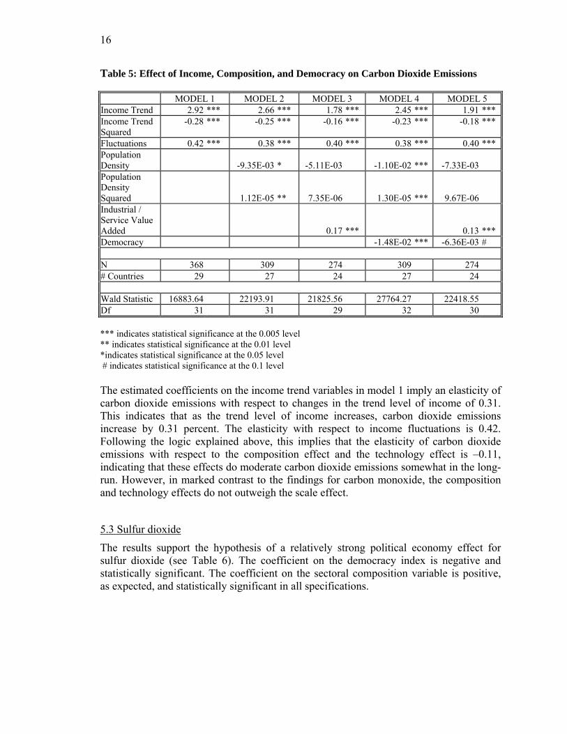
The political economy effect is expected to be relatively weak for carbon dioxide emissions, due to the global character of the associated externalities. The results for CO2 are shown in Table 5. The estimated coefficients on the income trend and its square again indicate an inverted-U relationship, which is consistent with other studies (see, for example, Stern (2002)). However, the turning point occurs at about $17,400 (in 1987 international dollars), a level corresponding to the per capita income of the United States in the 1990s. The fact that the turning point occurs at so high a level of income does not bode well for those who hope that economic growth will reduce worldwide carbon dioxide emissions in the foreseeable future. The estimated coefficients on population density and the sectoral composition variable have the expected signs. When sectoral composition is included as an explanatory variable, the estimated coefficient on the democracy index is of marginal statistical significance (though it does have the expected negative sign).

16

Table 5: Effect of Income, Composition, and Democracy on Carbon Dioxide Emissions MODEL 1 MODEL 2 MODEL 3 MODEL 4 MODEL 5 Income Trend 2.92 *** 2.66 *** 1.78 *** 2.45 *** 1.91 *** Income Trend Squared

-0.28 *** -0.25 *** -0.16 *** -0.23 *** -0.18 ***

Fluctuations 0.42 *** 0.38 *** 0.40 *** 0.38 *** 0.40 *** Population Density

-9.35E-03 * -5.11E-03 -1.10E-02 *** -7.33E-03


1.12E-05 ** 7.35E-06 1.30E-05 *** 9.67E-06


0.17 *** 0.13 *** Democracy -1.48E-02 *** -6.36E-03 #

N 368 309 274 309 274 # Countries 29 27 24 27 24

Wald Statistic 16883.64 22193.91 21825.56 27764.27 22418.55 Df 31 31 29 32 30

*** indicates statistical significance at the 0.005 level ** indicates statistical significance at the 0.01 level *indicates statistical significance at the 0.05 level # indicates statistical significance at the 0.1 level The estimated coefficients on the income trend variables in model 1 imply an elasticity of carbon dioxide emissions with respect to changes in the trend level of income of 0.31. This indicates that as the trend level of income increases, carbon dioxide emissions increase by 0.31 percent. The elasticity with respect to income fluctuations is 0.42. Following the logic explained above, this implies that the elasticity of carbon dioxide emissions with respect to the composition effect and the technology effect is –0.11, indicating that these effects do moderate carbon dioxide emissions somewhat in the long-run. However, in marked contrast to the findings for carbon monoxide, the composition and technology effects do not outweigh the scale effect.

5.3 Sulfur dioxide

The results support the hypothesis of a relatively strong political economy effect for sulfur dioxide (see Table 6). The coefficient on the democracy index is negative and statistically significant. The coefficient on the sectoral composition variable is positive, as expected, and statistically significant in all specifications.

17

Table 6: Effect of Income, Composition, and Democracy on Sulfur Dioxide Emissions

MODEL 1 MODEL 2 MODEL 3 MODEL 4 MODEL 5 Income Trend 8.18 *** 8.16 *** 7.40 *** 7.22 *** 6.62 *** Income Trend Squared

-1.01 *** -0.99 *** -0.99 *** -0.91 *** -0.91 ***

Fluctuations 0.42 *** 0.49 *** 0.31 * 0.39 *** 0.24 * Population Density -4.81E-02 *** 6.72E-04 -4.50E-02 *** 7.87E-04Population Density Squared

3.18E-05 *** -1.57E-05 2.90E-05 ** -1.54E-05


0.37 *** 0.35 ***

Democracy -1.35E-02 *** -9.57E-03 ***

N 434 323 272 319 268# Countries 33 30 26 29 25

Wald Statistic 1085.32 3426.17 3032.67 3942.46 3234.75Df 35 34 31 34 31

*** indicates statistical significance at the 0.005 level ** indicates statistical significance at the 0.01 level *indicates statistical significance at the 0.05 level # indicates statistical significance at the 0.1 level The coefficients on the income and income squared terms again describe an inverted-U relationship for sulfur dioxide emissions. The turning point occurs at $5,700 in 1987 international dollars, a level of income roughly equivalent to that of Hungary.11 In model 1, the elasticity of sulfur dioxide emissions with respect to trend income is -0.93. The elasticity of sulfur dioxide emissions with respect to income fluctuations is 0.42. Hence the elasticity of emissions with respect to the composition and technology effects of income growth is –1.35. This indicates that the latter effects together have contributed to a substantial decrease in per capita sulfur dioxide emissions.

5.4 Volatile organic compounds

The results for volatile organic compounds, reported in Table 7, support the hypothesis that the political economy effect, as proxied by the estimated coefficient on the democracy index, will be weaker than in the case of sulfur dioxide. Nevertheless, it is statistically significant, with the expected sign. The estimated coefficient on the composition variable is positive and statistically significant, also as expected.

11 Selden and Song (1994) estimated a turning point of $8,900 in 1985 US$; Grossman and Krueger (1995) arrived at a turning point of under $5,000, also in 1985 US$.

18

Table 7: Effect of Income, Composition, and Democracy on Volatile Organic Compound Emissions

MODEL 1 MODEL 2 MODEL 3 MODEL 4 MODEL 5

Income Trend 3.28 *** 2.20 *** 1.71 *** 2.04 *** 1.61 *** Income Trend Squared

-0.35 *** -0.17 *** -0.12 * -0.16 * -0.12 #

Fluctuations 0.48 *** 0.26 *** 0.19 * 0.21 *** 0.18 * Population Density

-5.16E-02 *** -6.75E-02 *** -4.83E-02 *** -7.09E-02 ***


4.20E-05 *** 6.24E-05 *** 3.86E-05 *** 6.65E-05 *** Industrial / Service Value Added

0.20 *** 0.13 *** Democracy -9.33E-03 *** -8.21E-03 **

N 344 259 222 255 218 # Countries 32 29 25 28 24

Wald Statistic 2324.99 3248.34 7522.82 2908.25 5521.95 Df 34 33 30 33 30

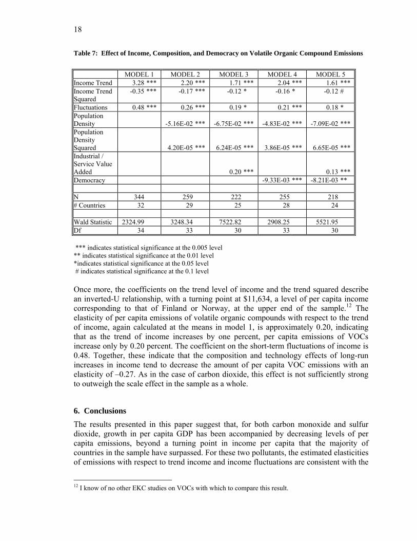
*** indicates statistical significance at the 0.005 level ** indicates statistical significance at the 0.01 level *indicates statistical significance at the 0.05 level # indicates statistical significance at the 0.1 level Once more, the coefficients on the trend level of income and the trend squared describe an inverted-U relationship, with a turning point at $11,634, a level of per capita income corresponding to that of Finland or Norway, at the upper end of the sample.12 The elasticity of per capita emissions of volatile organic compounds with respect to the trend of income, again calculated at the means in model 1, is approximately 0.20, indicating that as the trend of income increases by one percent, per capita emissions of VOCs increase only by 0.20 percent. The coefficient on the short-term fluctuations of income is 0.48. Together, these indicate that the composition and technology effects of long-run increases in income tend to decrease the amount of per capita VOC emissions with an elasticity of –0.27. As in the case of carbon dioxide, this effect is not sufficiently strong to outweigh the scale effect in the sample as a whole.

6. Conclusions The results presented in this paper suggest that, for both carbon monoxide and sulfur dioxide, growth in per capita GDP has been accompanied by decreasing levels of per capita emissions, beyond a turning point in income per capita that the majority of countries in the sample have surpassed. For these two pollutants, the estimated elasticities of emissions with respect to trend income and income fluctuations are consistent with the

12 I know of no other EKC studies on VOCs with which to compare this result.

18

conclusion that the composition and technology effects associated with income growth have outweighed the scale effect. These results are summarized in Table 8. For carbon dioxide and VOCs, in contrast, the results show turning points at the high end of the sample’s income range. Hence emissions generally rise as the trend level of income increases, implying that the composition and technology effects were not strong enough to outweigh the scale effects.

Table 8: Summary of Estimated Elasticities

ESTIMATED ELASTICITY OF EMISSIONS WITH RESPECT TO: POLLUTANT

Income trenda Income Fluctuationsb

Sectoral Compositionc Democracyd

CO -0.33 0.25 0.09 -0.09 CO2 0.31 0.42 0.11 -0.13 SO2 -0.93 0.42 0.25 -0.11 VOC 0.20 0.48 0.13 -0.07 a Elasticity = β1 + 2β2[mean(ln(income)]. b Elasticity = β3. Estimated from model 1. c Elasticity = β6/[mean(POL)/mean(ln(INDSERV))]. Estimated from model 3. d Elasticity = β7/[mean(POL)/mean(ln(DEMOC))]. Estimated from model 4. Attempting to disaggregate these effects further, the results indicate that the sectoral composition effect invariably played an important part in emission reductions: a higher ratio of value added from the industrial sector to that from the service sector was associated with increased emissions in all cases. The elasticity of emissions with respect to the sectoral composition variable (estimated at the means from model 3), was greatest in the case of sulfur dioxide, with an elasticity of 0.25, followed by VOCs (0.13), carbon dioxide (0.11), and CO (0.09). The democracy index, a measure of access to government, is here regarded as a proxy for the induced policy response component of the technology effect. It also proved to play a statistically significant role in all emissions studied. The elasticity (estimated at the means from model 4) was greatest in absolute value in the case of carbon dioxide (–0.13), followed by sulfur dioxide (–0.11), carbon monoxide (–0.09), and VOCs (–0.07). These results are somewhat surprising, in that carbon dioxide, as a global public bad, was hypothesized to have a weaker political economy effect. However, the estimated elasticity for carbon dioxide is within one standard deviation of that for sulfur dioxide, so the difference between the estimates is not statistically significant. The estimated coefficient on the income fluctuation variable was positive and statistically significant in all specifications for all contaminants. The elasticities of emissions with respect to this variable (estimated at the means from model 1), ranged from 0.25 to 0.48, suggesting that the scale effect, captured by income fluctuations, is not a one-to-one

19

correspondence. This finding is consistent with the view that pollution has a “fixed cost” as well as a “variable cost” component; while the latter tracks short-run income fluctuations, the former does not. These results reinforce the need for caution in the analysis of the income-degradation relationship. To be sure, there is evidence that as a country develops, the share of its manufacturing sector in GDP falls and democracy strengthens. Both of these contribute to reductions in emissions. But these effects have not been sufficiently strong to offset the scale effect in carbon dioxide and volatile organic compound emissions. Moreover, as Arrow et al. (1995) caution, if the developing countries cannot follow the “clean growth” trajectory that ostensibly has characterized the developed nations, then becoming richer may not improve their environmental quality. The findings reported here suggest that environmental improvements are especially unlikely if the growth process is heavy on manufacturing and light on democracy. ACKNOWLEDGEMENTS

The author wishes to thank James K. Boyce, Michael Ash, Bernie Morzuch, and the participants in the Environmental Working Group at the Political Economy Research Institute, University of Massachusetts, Amherst, for helpful comments on earlier incarnations of this work.

20

REFERENCES

Arrow, K. et al. 1995. “Economic growth, carrying capacity and the environment,” Science 268: 520-521. Baldson, Ed. 2003. “Political economy and the decomposition of environmental income effects,” Discussion paper 03-03. Department of Economics, Center for Public Economics, San Diego State University. Barrett, S. and K. Graddy. 2000. “Freedom, Growth, and the Environment,” Environment and Development Economics 5:433-56. Beckerman, W. 1992. “Economic growth and the environment: Whose growth? Whose environment?” World Development 20: 481-496. Brookhaven National Laboratory, 2002. “Volatile Organic Compounds: Historical use leads to concerns,” Cleanupdate 3(2). Available on line at: www.bnl.gov/erd/cleanupdate/vol3no2/vocs32.html. Environmental Protection Agency. 2003.“Sulfur Dioxide.” Available on line at www.epa.gov/air/sixpol.html. European Opinion Research Group. 2002. "Eurobarometer 58.0: The attitudes of Europeans towards the environment." Gallup Organization, CNN, and USA Today, “Public concern about pollution and identification with environmentalism has dropped in the past decade.” Available on line. Accessed at: http://www.publicagenda.org/issues/pcc.cfm?issue_type=environment Grossman, G. and A. Krueger. 1995. “Economic growth and the environment,” Quarterly Journal of Economics 112: 353-378. Heerink, N., A. Mulatu, and E. Bulte. 2001. “Aggregation bias and the environmental Kuznets curve,” Ecological Economics 38:359-67. Herbert, F. 2003. “Documents reveal that EPA downplayed climate change in a report on environmental challenges,” Environmental News Network, June 20. Accessed on line at www.enn.com. Hicks, Richard. 1939. Value and Capital: An Inquiry into Some Fundamental Principles of Economic Theory (Oxford: Clarendon Press). Jaffe, A. et al. 1995. “Environmental regulation and the competitiveness of U.S. manufacturing: What does the evidence tell us?” Journal of Economic Literature 33:132-63.

http://www.bnl.gov/erd/cleanupdate/vol3no2/vocs32.html

http://www.epa.gov/air/sixpol.html

http://www.publicagenda.org/issues/pcc.cfm?issue_type=environment

21

Jayadevappa, R. and S. Chhatre. 2000. “International trade and environmental quality: A survey,” Ecological Economics 32(2):175-194. Kahn, M. 1995. “Micro evidence on the environmental Kuznets curve.” Working Paper, Columbia University. Khalil, M.A.K. 1995. “Decline in atmospheric carbon monoxide raises questions about its cause,” Earth in Space 8(3): 7. Marshall, M. and K. Jaggers. 2002. “Polity IV Project: Political regime characteristics and transitions, 1800 –2002: Dataset users’ manual.” Center for International Development and Conflict Management. Available on line at www.cidcm.umd.edu/inscr/polity. Occupational Safety and Health Administration (OSHA), 2002. “Carbon Monoxide Fact Sheet.” Available at www.osha.gov. Scruggs, L. 1998. “Political and Economic Inequality and the Environment,” Ecological Economics 26 (3), 1998, 259-75.

Selden, T. and D. Song. 1994. “Environmental quality and development: Is there a Kuznets curve for air pollution?” Journal of Environmental Economics and Management 27: 147-162.

Stern, D. 2002. “Explaining changes in global sulfur emissions: An econometric decomposition approach,” Ecological Economics 42: 201-220. Torras, M. and J. Boyce. 1998. “Income, Inequality, and Pollution: A Reassessment of the Environmental Kuznets Curve,” 25:147-160. World Almanac Book of Facts. 2003. “Air Pollution,” page166. Accessed on line in Academic Search Premier. World Bank. 1992. World Development Report 1992. World Development Indicators. 1999. CD-ROM. World Resources Institute. 2001. “Searchable Database.” Accessed at http://earthtrends.wri.org.

http://www.osha.gov/

http://earthtrends.wri.org/

22

M

Armenia Austria Belarus Belgium Bulgaria Canada Cyprus Czech Rep Denmark Finland France Germany Greece Hungary Iceland Ireland Italy Latvia Lithuania Luxembourg Moldova, Rep Netherlands Norway Poland Portugal Romania Russian Federation Slovakia Slovenia Spain Sweden Switzerland Ukraine United Kingdom United States

Appendix Table 1: Countries included in databases

Carbon onoxide

Carbon Dioxide

Sulfur Dioxide Volatile Organic Compounds