energy efficient small cell planning for high capacity
TRANSCRIPT

University of North DakotaUND Scholarly Commons
Theses and Dissertations Theses, Dissertations, and Senior Projects
January 2015
Energy Efficient Small Cell Planning For HighCapacity Wireless NetworksMd Maruf Ahamed
Follow this and additional works at: https://commons.und.edu/theses
This Thesis is brought to you for free and open access by the Theses, Dissertations, and Senior Projects at UND Scholarly Commons. It has beenaccepted for inclusion in Theses and Dissertations by an authorized administrator of UND Scholarly Commons. For more information, please [email protected].
Recommended CitationAhamed, Md Maruf, "Energy Efficient Small Cell Planning For High Capacity Wireless Networks" (2015). Theses and Dissertations.1732.https://commons.und.edu/theses/1732

ENERGY EFFICIENT SMALL CELL PLANNING FOR HIGH CAPACITY WIRELESS NETWORKS
by
Md. Maruf Ahamed
Bachelor of Science in Electronics & Telecommunication Engineering, Rajshahi
University of Engineering & Technology, 2010
A Thesis
Submitted to the Graduate Faculty
of the
University of North Dakota
in partial fulfillment of the requirements
for the degree of
Master of Science
Grand Forks, North Dakota
August
2015

ii
Copyright 2015 Md. Maruf Ahamed

iii

iv
PERMISSION
Title Energy Efficient Small Cell Planning for High Capacity Wireless
Networks
Department Electrical Engineering
Degree Master of Science
In presenting this thesis in partial fulfillment of the requirements for a graduate
degree from the University of North Dakota, I agree that the library of this University
shall make it freely available for inspection. I further agree that permission for extensive
copying for scholarly purposes may be granted by the professor who supervised my
thesis work or, in his absence, by the chairperson of the department or the dean of the
Graduate School. It is understood that any copying or publication or other use of this
thesis or part thereof for financial gain shall not be allowed without my written
permission. It is also understood that due recognition shall be given to me and to the
University of North Dakota in any scholarly use which may be made of any material in
my thesis.
Signature Md. Maruf Ahamed
Date 07/10/2015

v
TABLE OF CONTENTS
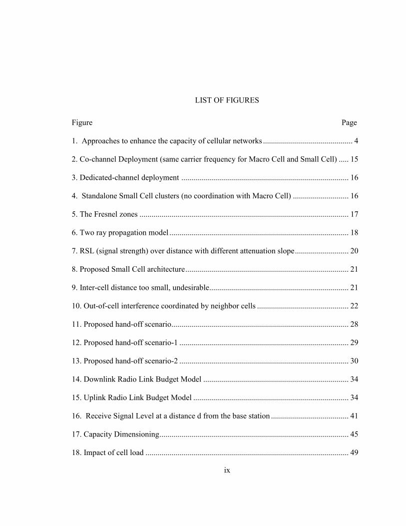
LIST OF FIGURES ............................................................................................... ix
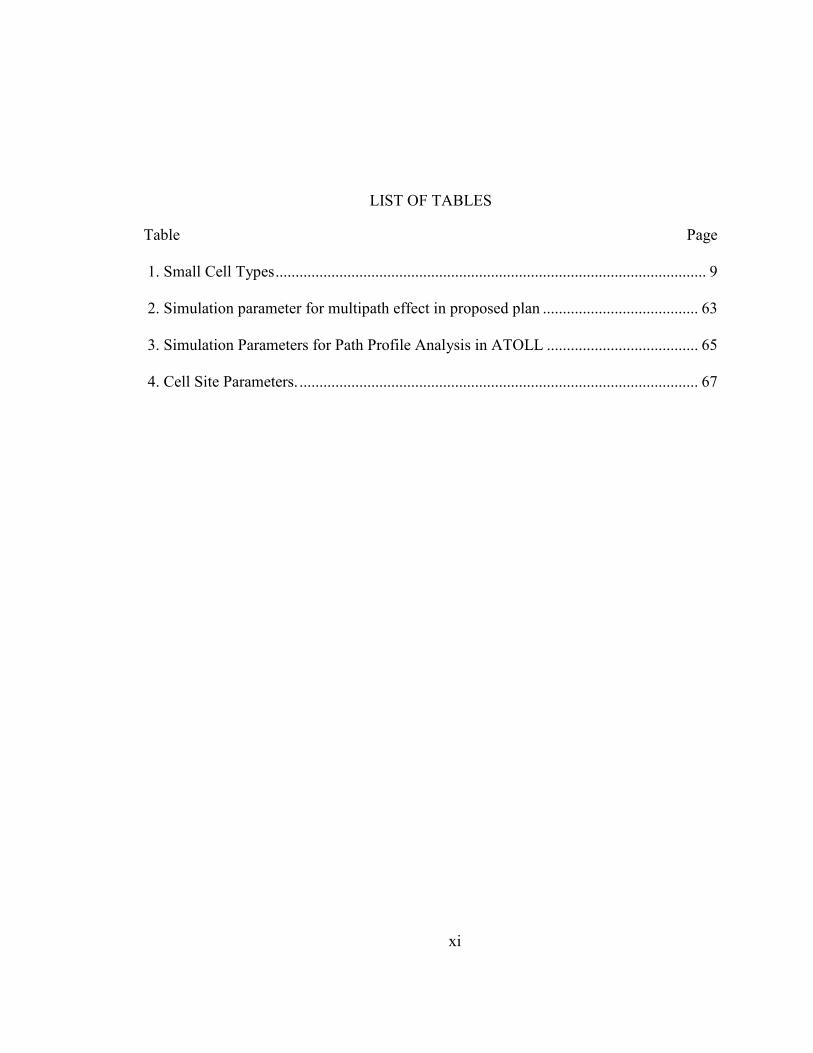
LIST OF TABLES ................................................................................................. xi
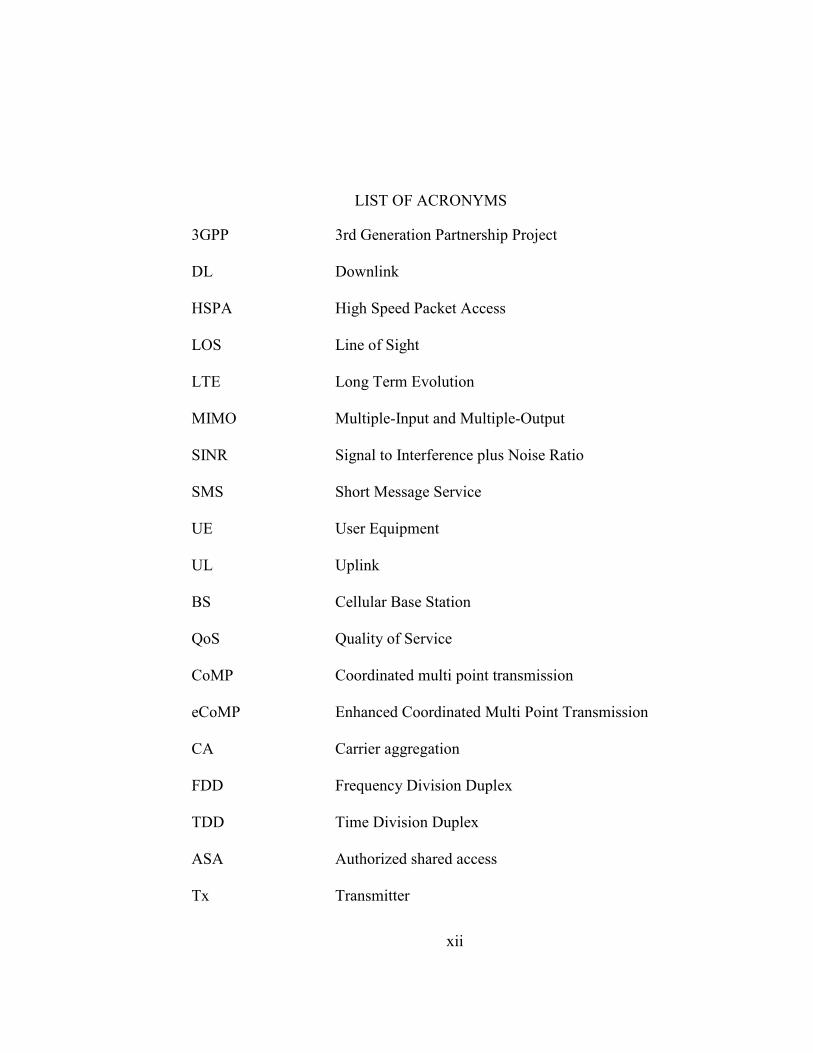
LIST OF ACRONYMS ......................................................................................... xi
ACKNOWLEDGEMENTS ................................................................................. xiv
ABSTRACT .......................................................................................................... xv
CHAPTER
1. INTRODUCTION ...................................................................................... 1
2. SMALL CELL NETWORKS OVERVIEW .............................................. 3
2.1 Motivation to Deploy Small Cells ....................................................... 3
2.1.1 Enhance Macro Layer Efficiency .......................................... 3
2.1.2 Densifying the Macro Network ............................................. 7
2.2 Introducing Small Cell Networks ........................................................ 7
2.3 Types of Small Cells ............................................................................ 8
2.3.1 Macro Cells/ Micro Cells ....................................................... 9
2.3.2 Pico Cells ............................................................................... 9
2.3.3 Femtocells ............................................................................ 10
2.4 Small Cell Networks Deployment Challenges ................................... 10
2.4.1 Backhauling ......................................................................... 10

vi
2.4.2 Handover .............................................................................. 11
2.4.3 Self-Organizing Networks ................................................... 12
2.4.4 Interference .......................................................................... 12
3. DENSE SMALLC ELL DEPLOYMENT ................................................ 14
3.1 Introduction ........................................................................................ 14
3.2 Small Cell Deployment Scenario ....................................................... 15
3.3 Proposed Small Cell Architecture ...................................................... 16
3.3.1 Overview of Fresnel Zone Effect ......................................... 16
3.3.2 Proposed Small Cell Architecture ........................................ 20
3.3.3 Propagation Prediction Model for Proposed Architecture ... 23
4. CELL SELECTION AND HANDOVER IN SMALL CELL NETWORKS .................................................................................................................. 25
4.1 Introduction ........................................................................................ 25
4.2 Conventional Cell Selection Methods ............................................... 26
4.2.1 RSRP-Based Cell Selection ................................................. 26
4.2.2 RSRQ-Based Cell Selection ................................................ 27
4.3 Proposed Cell Selection and Hand-Off Mechanism .......................... 28
4.4 Performance Analysis of Proposed Hand-Off Mechanism ................ 29
4.4.1 Scenario-1: When Small Cell Very Close to Macro Cell .... 29
4.4.2 Scenario-2: When Two Small Cells Are Very Close........... 30
5. COVERAGE AND CAPACITY DIMENSIONING ............................... 31
5.1 Coverage Planning ............................................................................. 31
5.1.1 Radio Link Budget ............................................................... 32
5.1.2 Coverage Analysis ............................................................... 40

vii
5.1.3 Okumura-Hata Propagation Prediction Model .................... 42
5.2 Capacity Planning .............................................................................. 44
5.2.1 Number of Sites due to Coverage ........................................ 45
5.2.2 Number of Sites due to Capacity ......................................... 46
5.3 Factors Affecting the Cell Capacity ................................................... 47
5.3.1 Cell Range (Pathloss) ........................................................... 48
5.3.2 Channel Bandwidth .............................................................. 48
5.3.3 Cell Load .............................................................................. 48
6. INTERFERENCE IN SMALL CELL NETWORKS ............................... 50
6.1 Interference Challenge ....................................................................... 50
6.1.1 Power Difference ................................................................. 51
6.1.2 Unplanned Deployment ....................................................... 52
6.1.3 Closed Subscriber Group (CSG) Access ............................. 52
6.2 Small Cell Interference Scenarios ...................................................... 52
6.2.1 Macro Cell Downlink to the Small Cell UE Interference .... 53
6.2.2 Macro Cell UE Uplink to the Small Cell Interference ....... 53
6.2.3 Small Cell Downlink to the Macro Cell UE ....................... 54
6.2.4 Small Cell UE Uplink to the Macro Cell Interference ......... 55
6.2.5 Small Cell Downlink to the nearby Small Cell UE ............ 56
6.2.6 Small Cell UE Uplink to the nearby Small Cell ................. 57
6.3 Interference Coordination in Heterogeneous Networks .................... 57
6.3.1 Frequency Domain Techniques ........................................... 58
6.3.2 Time Domain Techniques .................................................... 59

viii
6.3.3 Power Control Based Solution ............................................. 60
7. SIMULATION AND RESULT ................................................................ 61
7.1 Calculating Small Cell Radius ........................................................... 61
7.2 Multipath Effect in Proposed plan ..................................................... 63
7.3 Path Profile Analysis.......................................................................... 65
7.4 Coverage Analysis of Heterogeneous Networks ............................... 67
7.5 Capacity Analysis of Heterogeneous Networks ................................ 69
7.6 Carrier to Interference (C/I) Improvement ........................................ 70
8. CONCLUSION & FUTURE WORK ....................................................... 72
REFERENCES ..................................................................................................... 81
ix
LIST OF FIGURES
Figure Page
1. Approaches to enhance the capacity of cellular networks ............................................. 4
2. Co-channel Deployment (same carrier frequency for Macro Cell and Small Cell) ..... 15
3. Dedicated-channel deployment .................................................................................... 16
4. Standalone Small Cell clusters (no coordination with Macro Cell) ............................ 16
5. The Fresnel zones ......................................................................................................... 17
6. Two ray propagation model .......................................................................................... 18
7. RSL (signal strength) over distance with different attenuation slope ........................... 20
8. Proposed Small Cell architecture .................................................................................. 21
9. Inter-cell distance too small, undesirable...................................................................... 21
10. Out-of-cell interference coordinated by neighbor cells .............................................. 22
11. Proposed hand-off scenario......................................................................................... 28
12. Proposed hand-off scenario-1 ..................................................................................... 29
13. Proposed hand-off scenario-2 ..................................................................................... 30
14. Downlink Radio Link Budget Model ......................................................................... 34
15. Uplink Radio Link Budget Model .............................................................................. 34
16. Receive Signal Level at a distance d from the base station ....................................... 41
17. Capacity Dimensioning ............................................................................................... 45
18. Impact of cell load ...................................................................................................... 49

x
19. Problem caused by difference in power between Macro and Small Cells .................. 51
20. Macro Cell Downlink to the Small Cell UE Interference ........................................... 53
21. Macro Cell UE Uplink to the Small Cell Interference ................................................ 53
22. Small Cell Downlink to the Macro Cell UE Interference ........................................... 54
23. Small Cell UE Uplink to the Macro Cell Interference ................................................ 55
24. Small Cell UE Uplink to the Macro Cell Interference (Example) .............................. 55
25. Small Cell downlink to the nearby Small Cell UE Interference ................................. 56
26. Small Cell UE Uplink to the nearby Small Cell Interference ..................................... 57
27. Frequency domain eICIC Techniques ........................................................................ 58
28. Time domain eICIC Techniques. ................................................................................ 59
29. Fresnel zone break point varies with Tx height (F=2100MHz, h1=1.5m) ................. 61
30. Fresnel zone break point varies with TX Height (h1=1.5m, h2=20M) ...................... 62
31. Fresnel zone break point varies with Tx height (h1=1.5m, h2=20M) ........................ 63
32. Indoor cell radius as a function of attenuation slope .................................................. 64
33. Outdoor cell radius as a function of attenuation slope ................................................ 64
34. Path profile analysis scenario-1 for Macro Cell. ........................................................ 66
35. Path profile analysis scenario -2 for Macro Cell ........................................................ 66
36. Path profile analysis for Small Cell ............................................................................ 66
37. Heterogeneous Networks coverage for Macro only deployment. .............................. 67
38. Heterogeneous Network coverage with Small Cell deployment ................................ 68
39. Heterogeneous Network capacity for Macro only (Total users=735) ........................ 69
40. Heterogeneous Network capacity with Small Cell .................................................... 70
41. Carrier to Interference for different path loss slope .................................................... 71
xi
LIST OF TABLES
Table Page
1. Small Cell Types ............................................................................................................ 9
2. Simulation parameter for multipath effect in proposed plan ....................................... 63
3. Simulation Parameters for Path Profile Analysis in ATOLL ...................................... 65
4. Cell Site Parameters. .................................................................................................... 67
xii
LIST OF ACRONYMS
3GPP 3rd Generation Partnership Project
DL Downlink
HSPA High Speed Packet Access
LOS Line of Sight
LTE Long Term Evolution
MIMO Multiple-Input and Multiple-Output
SINR Signal to Interference plus Noise Ratio
SMS Short Message Service
UE User Equipment
UL Uplink
BS Cellular Base Station
QoS Quality of Service
CoMP Coordinated multi point transmission
eCoMP Enhanced Coordinated Multi Point Transmission
CA Carrier aggregation
FDD Frequency Division Duplex
TDD Time Division Duplex
ASA Authorized shared access
Tx Transmitter

xiii
Rx Receiver
CSG Closed subscriber group
DSL Digital subscriber lines
SON Self-organizing network
DSL Digital Subscriber Line
HetNet Heterogeneous Networks
RSRQ Reference Signal Received Quality
RSSI Received signal strength indicator
TAI Tracking area indicator
RSL Received signal level
RLB Radio Link Budget
eNodeB E-UTRAN Node B
OFDMA Orthogonal Frequency-Division Multiple Access
QPSK Quadrature Phase-Shift Keying
QAM Quadrature Amplitude Modulation
RF Radio Frequency
SC Small Cell
eICIC Enhanced inter-cell interference coordination
ICIC Inter-cell interference coordination
CRE Cell range expansion
ABS Almost blank sub frames
C/I Carrier-to-interference ratio
RSRP Reference signal received power

xiv
ACKNOWLEDGEMENTS
I would first like to express my gratitude to my advisor, Dr. Saleh Faruqe for his
guidance, support, and encouragement. His belief in my judgment and abilities has helped
me to stay focused on my goals and motivated me to achieve them.
I would also like to thank my committee members, Dr. Sima Noghanian, and Dr.
Prakash Ranganathan for their invaluable comments and suggestions.
I thank the Electrical Engineering Department at the University of North Dakota
for giving me this opportunity and financial support to finish my thesis.
Furthermore, I would like to acknowledge Rockwell Collins for partially funding
this research work.
In particularly, I am very grateful to my family for their love and support.

To my family.

xv
ABSTRACT
This thesis presents a new strategy to densify Small Cells (i.e., add more low
powered base stations within macro networks) and enhance the coverage and capacity of
Heterogeneous Networks. This is accomplished by designing Micro Cell for outdoor
applications, Pico and Femtocell for indoor applications. It is shown that, there exists a free
space propagation medium in all propagation environments due to Fresnel zones, and the
path loss slope within this zone is similar to free space propagation medium. This forms
the basis of our development of the present work. The salient feature of the proposed work
has two main considerations (a) The cell radius of Small Cells must be within the first
Fresnel zone break point, and (b) The minimum inter-cell distance must be greater than
twice of Small Cell radius.
The proposed network is simulated in real a radio network simulator called
ATOLL. The simulation results showed that densify Small Cells not only enhanced the
capacity and coverage of Heterogeneous Networks but also improved the carrier to
interference ratio significantly. Since the proposed work allows UE (user equipment) to
have Line of Sight (LOS) communication with the serving cell, and UE can have higher
uplink (UL) signal to interference plus noise ratio (SINR) that will further allow UE to
reduce its transmission power, which will consequently lead to a longer battery life for the
UE and reduce the interference in the system.
1
CHAPTER 1
INTRODUCTION
According to recent projections, mobile data traffic is getting doubled every year
and the estimated increase roughly by a factor of 1000 in the next 10 years [1]. This
increasing capacity requires fundamental changes in cellular network planning and
deployment [2]. Hence, the service providers need to add more capacity with significantly
lower cost per bit. New ways to enhance the revenue are also of interest to the service
providers [3].
There are three main approaches to cope this data demand: (i) network
densification: by deployment of Small Cells, (ii) adding more bandwidth: wider bandwidth
that is realistic at millimeter wave frequencies, and (iii) improving spectral efficiency: by
using advanced radio access technology, such as Long Term Evolution (LTE), and utilizing
special features like massive-multiple-input and multiple-output (MIMO), and better
interference management techniques. The last two approaches are certainly important
pieces of the puzzle [4], the most of the gains can be achieved by network densification.
This thesis presents different deployment scenarios of Small Cells and propose a
method to deploy Small Cells densely within or outside of macro layer and enhance the
coverage and capacity of heterogeneous networks.

2
It is shown that, there exists a free space propagation medium in all propagation
environments due to Fresnel zones, that the path loss slope within this zone is similar to
that of free space propagation medium. The salient feature of the proposed work has two
main considerations (a) the cell radius of Small Cells must be within the first Fresnel zone
break point, and (b) the minimum inter-cell distance must be greater than twice of Small
Cell radius.
This thesis also investigates mobility management problems in Heterogeneous
Networks and propose a new cell selection scheme called path loss slope based cell
selection, where a UE (user equipment) selects the best cell based on the path loss slope
value of the received signal instead of the received signal level. The performance of the
proposed cell selection scheme is also shown and compared with conventional cell
selection schemes. Finally, it is proved that, conventional cell selection schemes are no
longer sufficient when Small Cells are densely deployed for indoor or outdoor scenarios.
This thesis is organized as follows. Chapter 2 represents the motivation to deploy
Small Cells and brief overview of Small Cell networks. Different deployment scenarios of
Small Cells are discussed in chapter 3.The proposed Small Cell architecture is also
proposed in this chapter. In chapter 4 different cell selection methods are discussed and a
new cell selection method based on the path loss slope value of received signal is proposed.
In addition, coverage and capacity planning are discussed in chapter 5 and interference in
Small Cell networks are discussed in chapter 6. Finally simulation and results are shown
in chapter 7. In chapter 8, some conclusions are drawn.

3
CHAPTER 2
SMALL CELL NETWORKS OVERVIEW
2.1 Motivation to Deploy Small Cells
Until 2010, cellular network was planned to support voice calls and Short Message
Service (SMS). The reliable delivery of 15 kbps or so was enough to keep an end user
happy. But the game has changed in the last few years due to the rapid growth of mobile
broadband traffic, driven by the growing adoption of the data hungry multimedia services.
Since the popularity of connecting devices (e.g., smartphones and tablets) has increased,
the data-rate demands per user has increased dramatically [5]. According to recent
projections, mobile data traffic is getting doubled every year and the estimated increase of
1000 times in the next 10 years [6, 7]. Hence, the service providers need to add more
capacity with significantly lower cost per bit and finding some ways to enhance the revenue
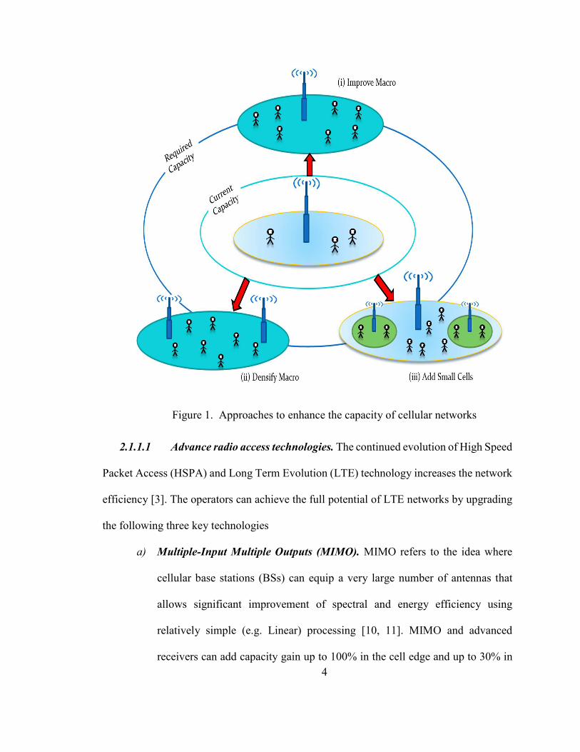
as well [7]. There are several approaches to meet this traffic demand, shown in Figure 1.
The Traditional approaches are explained in the following [8, 9]:
2.1.1 Enhance Macro Layer Efficiency
Improving the existing Macro Network can be a possible way to enhance the
capacity of macro network. This can be done by using advanced radio access technologies
or by adding more spectrums in the macro networks, as discussed below.
4
Figure 1. Approaches to enhance the capacity of cellular networks
2.1.1.1 Advance radio access technologies. The continued evolution of High Speed
Packet Access (HSPA) and Long Term Evolution (LTE) technology increases the network
efficiency [3]. The operators can achieve the full potential of LTE networks by upgrading
the following three key technologies
a) Multiple-Input Multiple Outputs (MIMO). MIMO refers to the idea where
cellular base stations (BSs) can equip a very large number of antennas that
allows significant improvement of spectral and energy efficiency using
relatively simple (e.g. Linear) processing [10, 11]. MIMO and advanced
receivers can add capacity gain up to 100% in the cell edge and up to 30% in

5
cell center [12]. MIMO implemented using diversity techniques that provide
diversity gain and improves the system reliability. In addition, massive MIMO
(also known as a large scale antenna system, very large MIMO, and hyper
MIMO) brings huge improvements in throughput and radiated energy
efficiency.
b) Smart scheduling. In case of conventional LTE schedulers, radio resources are
allocated to active subscribers in each cell, hence substantial spectrum remains
unallocated. On the other hand, smart scheduler assigns spectrum blocks to
users in every millisecond based on their application demands and required
quality of service (QoS). Smart scheduling can mitigates inter-cell interference
and improve cell capacity by more than 20%. It can also boost cell edge data
rates by more than 100% and can achieve more than 50% average throughput
than conventional LTE schedulers [3].
c) Coordinated multi point transmission (CoMP). In a distributed network
architecture (e.g., LTE Release 8), data are transmitted to the mobile device
from one cell at a time [14]. But, CoMP is a facility of LTE advanced networks,
where multiple cells can transmit data to a single mobile device [15]. By
providing connections to multiple base stations at a time, data can be passed to
the least loaded base stations to enhance resource utilization. The overall
reception can also be improved by using several cell sites for each connection,
hence, the number of dropped calls is reduced. In addition, specialized
combining techniques allow utilizing the interference constructively, instead
of destructively, thereby interference is reduced. Further improvement can be

6
achieved by using enhanced Coordinated Multi Point Transmission (eCoMP),
which allows multi-cell resource control [13].
2.1.1.2 New spectrum and optimal use of spectrum. Maximizing the utilization of
existing spectrum or adding more spectrums into services can add more capacity in the
macro networks. There are three strategies to improve as follows:
a). Carrier aggregation. Carrier aggregation is one of the most distinct features
of LTE Advanced, which is being standardized by 3rd Generation Partnership
Project (3GPP) [17]. This feature allows scalable expansion of effective
bandwidth delivered to a user through simultaneous utilization of radio
resources across multiple carriers. This can be done by aggregating several
smaller contiguous or non-contiguous carriers [16]. For instance, a 100 MHz
system can be constructed using contiguous or non-contiguous 5 × 20 MHz.
Carrier aggregation is supported by the Frequency Division Duplex (FDD) and
Time Division Duplex (TDD) both and it guarantees to meet the high data
throughput required by each of them.
b). Deploy new spectrum. Operators are able to use the 700, 800, 900, 1800, 2100
and 2600 MHz bands (EU example) for LTE networks and HSPA capacity
upgrades by the next few years. Capacity gain is possible by integrating use of
TDD and FDD spectrum. For instance, unused TDD spectrum will initially
supplement downlink or uplink FDD capacity, and then efficient carrier
aggregation across technologies will further bridge local and wide area assets.
c). Authorized Shared Access (ASA). ASA is a regulatory approach for sharing
bands where usage is low, but not vacated fully by incumbent users [16]. ASA

7
balances the mobile network operators with those needs of legacy spectrum
users and enables the availability and licensed use spectrum with QoS.
2.1.2 Densifying the Macro Network
The second possible solution is to densify the macro network. A simple way to
densify the macro network could be adding more sectors per Macro Cells. Splitting cells
horizontally can create additional sectors. For instance, upgrading a three sector site into a
six-sector site can boost capacity by up to 80% and the coverage of up to 40%. Vertical
splitting is also possible by deploying active antennas for beamforming. Two independent
dynamic beamforming can deliver up to 65% more capacity, as well as better coverage
with high data rates. Another way to densify the macro network would be deploying more
Macro Cells within the networks.
However, reducing the inter-cell distance and adding more Macro Cell in the
network can only be pursued in a certain extent because finding a position for new Macro
Cells becomes increasingly difficult and expensive, especially in the city centers. Besides,
the number of handoff within a cell will increase due to more Macro Cells in the vicinity
and additional software will need for this handoff.
2.2 Introducing Small Cell Networks
Small Cells are radio access nodes that can operate in licensed and unlicensed
spectrum and are operated by low-power. These nodes are "too small" compared to a
traditional Macro Cell, they are named Small Cells. The typical radius of a Small Cell will
be less a kilometers, whereas a Macro Cell can have a range of a few tens of kilometers.

8
The most promising approach to meet high capacity demand is to add more Small
Cells within the macro network and distribute the traffic between Macro Cell and Small
Cell [18]. Data capacity of a cell is defined as the aggregated cell throughput per cell. With
the identical condition (e.g. same channel bandwidth), the aggregated cell throughput of a
cell will remain the same, regardless of the size of the cell. Therefore, the aggregated cell
throughput for Macro Cell, Micro Cell, Small Cell, and Femtocell are the same. This means
that the total capacity is inversely proportional to the square of the cell radius. For instance,
if the cell radius is reduced to half, the cell capacity will be quadrupled.
The cell capacity is a function of several variables such as user distribution, fading
characteristics, and traffic moving speed. Small Cell users are slowly moving and usually
are located closer to the cell center with less fading, so the aggregated cell throughput from
a Small Cell is higher than a Macro Cell. Thus, by splitting the traffic from one large cell
into multiple Small Cells, the actual achieved capacity gain will be higher than the square
law [17].
2.3 Types of Small Cells
According to the cell radius and transmit (Tx) power levels, wireless cells can be
categorized into Macro Cells, Micro Cells, Pico Cells, and Femtocells [5]. The actual cell
size does not only depends on the cell Tx power, but also depends on the position of the
antenna, antenna height, as well as the deployment environment, e.g. indoor or outdoor,
rural or urban environment [6]. Any of the cells can be a better candidate than others
depending on different deployment environments, the type of communications, and the
quality of services. Table 1 shows the different types of Small Cells with corresponding
cell radii and Tx power levels [7].

9
Table 1. Small Cell Types
Cell
Type
Cell Radius PA Power Rang &
Typical Value
Number
of UEs
Developed by Managed by
Macro >1Km 20W-160W
(40W)
1200 Operator Operator
Micro 250m–1Km 2W-20W (5W) 400 Operator Operator
Pico 100m-
300m
250mW~2W 64-256 Operator Operator
Femto 10m-50m 10mW-200mW 10-50 Consumer Consumer
2.3.1 Macro Cells/ Micro Cells
In current cellular networks, Macro Cells are deployed by operators for wide area
coverage and the coverage footprint varies for different traffic conditions. The typical inter-
site distance for Macro Cells are more than 500m in rural or suburban areas, while Micro
Cells are deployed in urban areas with smaller cell radius. In heterogeneous networks, large
Macro Cells hold advantages to support high mobility users and reduced handover
frequency [6].
2.3.2 Pico Cells
Pico Cells are deployed by the operator for smaller area coverage compared to
Micro Cells. It can be deployed in outdoor public venues and hotspots, especially in
capacity starved locations like stadiums, airports, and shopping malls [5]. The deployments
of Pico Cells are carefully planned by the operators, and are open and accessible by all

10
cellular users. Since, Pico Cells use lower Tx power than Micro Cells, it has reduced the
transmission cost [6].
2.3.3 Femtocells
Femtocells are usually privately owned unlike Micro Cells or Pico Cells and can be
deployed more efficiently based on user’s needs. A Femtocell covers even small areas (10-
50m), such as a house or an apartment [5]. Since Femtocells can connect to the network by
existing residential backhaul links such as cables or Digital Subscriber Lines (DSL), it can
save infrastructural cost [6]. Typically, Femtocells are under Closed Subscriber Group
(CSG) operation, where only specific users are allowed to access the network through
Femtocells [7]. This may cause interference to the network when sharing the same
spectrum with other tiers.
2.4 Small Cell Networks Deployment Challenges
Small Cells can be installed by subscribers, unlike traditional macro network
installed by operators [8, 9]. Thus, it introduces a significant network paradigm shift from
traditional centralized network to unplanned and uncoordinated network approaches. These
changes can be seen as a good approach for enhanced, however, they also entail some
technical challenges [5, 9]. The key deployment challenges of Small Cell networks are
discussed in this section.
2.4.1 Backhauling
Backhaul solution is needed for a network with large number of Small Cell sites.
Backhaul can be supported by a physical transmission medium, including microwave,
optical fiber, laser, copper lines, and wireless connectivity. Backhauling affects the data

11
throughput available for users, thus it affects the overall performance of the networks [5].
However, for more tight coordination’s of Small Cells and optimized uses of available
spectrum, a high performance backhaul with low latency is needed.
Since various types of cells can coexist in Small Cell networks, backhauling will
be a major issue to maintain the overall performance of the networks [5]. For instance, Pico
Cells require access to utility infrastructure with power supply and wired network
backhauling, which may be expensive [8]. On the other hand, Femtocell can use
consumer’s broadband connections for backhauling. This reduces dedicated backhauling
cost. But it may face difficulties to maintain quality of service (QoS) [9]. The operators
need to plan backhaul solution carefully to minimize the backhauling cost and also
guarantee the quality of service of the networks.
2.4.2 Handover
Handovers and mobility management are necessary in order to provide seamless
uniform services when users are moving around the different cell coverage [5]. Besides,
handovers are efficient to offload the traffic from highly congested cells to the less
congested neighbor cells [9]. In Small Cell networks, as the density of Small Cells increase,
the probability of handover increases. It is a challenge for Small Cell networks to reduce
signaling load to the core network and optimize handover performance. Small Cell
networks needed careful planning of handover parameters, which probably is different
from the traditional Macro Cells.

12
2.4.3 Self-Organizing Networks
One of the key features of the Small Cell networks is that users or operators can
deploy Small Cells without careful network planning [9]. The operators may not configure
individual Small Cells, but Radio Frequency (RF) environment will vary continuously after
Small Cells deployment. Hence each Small Cell needs to be monitored continuously for
any changes of the RF environment and reconfigure it if needed. Self-Organizing Network
(SON) possess an automated operation in cellular networks, and uses automated and
intelligent procedures to replace human intervention in the networks without
compromising the network performances. The key features of SONs can be categorized by
the following three processes [9, 19]:
a) Self-configuration: Newly deployed cells are automatically configured by the
software before the cells enter in the operational mode.
b) Self-healing: Cells can automatically perform failure recovery or execute
compensation mechanism whenever a failure occurs.
c) Self-optimization: Cells can continuously monitor the network status and can
optimize the network settings for better coverage and less interference
scenarios.
2.4.4 Interference
Unlike traditional single tier cellular networks, in heterogeneous networks, Small
Cells overly Macro Cells and originate new cell-boundaries, in which end users may suffer
strong inter-cell interference. In addition, different backhaul link solution with different
bandwidth and delay constraint for each cell may add more challenges for interference
13
coordination [9]. For instance, Pico Cells use X2 interface for exchanging signals, whereas
Femtocells use internet connection Digital Subscriber Line (DSL), thus delay issues may
appear [10]. The main reasons that cause interference in Small Cell networks and different
interference coordination methods are discussed in Chapter 6.

14
CHAPTER 3
DENSE SMALLC ELL DEPLOYMENT
3.1 Introduction
Innovative upgrades and new technology will significantly enhance the Macro
Cellular network capacity. Once Macro Cells reach their limits, Heterogeneous Networks
will be the norm to meet the high traffic demand. It is expected that more than 30 percent
of the world population will live in metro and urban areas by 2017. Although these areas
represent less than one percent of the Earth’s total land area, they will be the source of
around 60 percent of mobile traffic by 2017 [1]. Macro Cells are the proven cost effective
solution, but it will be increasingly challenging to meet the traffic demand in the following
scenarios, such as [2];
a). Large outdoor hotspots, such as commercial streets and town squares. If these
areas are already served by a dense macro network but still there is a high
growing traffic demand. The interference will also be high in those areas.
b). Large, isolated indoor hotspots, such as hotels and businesses. It will be
difficult to meet capacity and maintain the quality of service of the network.
c). Large indoor hotspots, such as airports, shopping malls, and subway stations,
where interference and mobility demands are high.

15
d). Localized indoor hotspots or minor coverage holes, such as retail outlets, small
offices, and restaurants. The deployment challenge will be the cost structure of
conventional cellular networks
In those outline scenarios; Small Cell networks will be a better solution than macro
network improvements, to maintain high quality user experience and provide good
coverage as well. Ericsson expects that each Macro Cell will on average have three
supporting Small Cells in metro and urban areas by 2017 [2].
3.2 Small Cell Deployment Scenario
Until LTE Release 12, the Small Cell deployments are considered in sparse
co-channel scenarios, but LTE Release 12 focuses mostly on dense Small Cell deployments
operating on separate carriers to the Macro Cell. The proposed work and simulation are
based on this scenario. Three deployment scenarios have been identified in LTE Release
12, (1) Small Cell deployed in the same carrier F1 as the Macro Cell, (2) Small Cell
deployed in carrier F2 different from the Macro Cell carrier F1, and (3) Standalone
deployment of Small Cells, as shown in Figures 2, 3 and 4 [6, 8, 20, 21, 22].
Figure 2. Co-channel Deployment (same carrier frequency for Macro Cell and Small Cell)

16
Figure 3. Dedicated-channel deployment (different carrier frequency for Macro Cell and
Small Cell)
Figure 4. Standalone Small Cell clusters (no coordination with Macro Cell)
3.3 Proposed Small Cell Architecture
3.3.1 Overview of Fresnel Zone Effect
When any wave-front encounters an obstacle it bends around the objects and spread
out when passing it through a gap. This phenomenon is known as diffraction [23].
Likewise, diffraction of radio waves occurs in multipath environment when the radio waves
encounter any obstacles [24]. This can be examined by a model developed by Augustin-
Jean Fresnel for optics [25]. Fresnel postulated that the cross-section of any optical

17
wavefront (electromagnetic wavefront) is divided into zones of concentric circles separated
by λ/2 (Figure 5), where λ is the wavelength.
Figure 5. The Fresnel zones
The radius of the nth Fresnel zone is given by
21
21
dd
ddnRn +
= λ (3.1)
Where, d1 is the distance between the transmitter and the obstruction, d2 is the
distance between the receiver and the obstruction, λ is the wavelength is equal to c/f where
c is velocity of light and f is the frequency, n = 1 for the first Fresnel zone, and n = 2 for
the second Fresnel zone.
Equation (3.1) indicates that the Fresnel zone radius is inversely proportional to the
square root of frequency. Thus, for a given antenna height, a high frequency signal will
propagate further before the first Fresnel zone touches the ground. Similarly, for a given

18
frequency, a signal that radiates from a tall antenna will propagate further before the first
Fresnel zone touches the ground. In short, diffraction of radio waves depends on frequency
as well as on antenna height. The maximum diffraction occurs when the path difference
between the direct ray and diffracted ray is λ/2. This can be verified by two-ray model,
show in below Figure 6.
Figure 6. Two ray propagation model
In Figure 6, h1 is the transmit (Tx) antenna height, h2 is the receive (Rx) antenna
height, d is the antenna separation, d1 is the length of reflected path, d2 is the length of
direct path. The path difference between direct and reflected path can be found according
to plane geometry as
2221
2221 )()( dhhdhhd +−−++=∆ (3.2)
Where, ∆d = d2 – d1. Equation (3.2) can be further rewritten as
1)(1)(
4
221221
21
+−
+++
=∆
d
hhd
d
hhd
hhd (3.3)

19
Where (h1 ± h2)/d << 1, the path difference in the equation (3.3) reduces to
d
hhd 212≠∆ (3.4)
Now the composite received can be expressed as
)]2
(sin4[)4
(]1[)4
( 2222 θπλ
πλ θ ∆=+= ∆
dPe
dPP T
j
Tr (3.5)
Where, PT is the power of the transmitted signal, Pr is the composite received power
and ∆θ is the phase difference between the direct and the reflected path. In terms of path
difference ∆θ is given by
d∆=∆ )2
(λπθ (3.6)
Thus equation (3. 5) can rewrite with the new value of ∆θ as
])(sin4[)4
( 22 dd
PP Tr ∆×=λπ
πλ
(3.7)
Further equation (3.7) can be rewrite by putting the value of ∆d from the equation
(3.4) as
}]2){(sin4[)4
( 2122
d
hh
dPP Tr ××=
λπ
πλ (3.8)
Pr will be maximum when sin2{(π/λ)×2h1h2/d} is maximized. Thus,
22 21 π
λπ =×
d
hh (3.9)
Or
�� = � = 4����
� (3.10)

20
Note that d is now replaced by d0 and this distance is known as Fresnel zone break
point which is proportional to antenna height and frequency. Therefore, it can conclude
that path loss characteristic within d0 will be similar to free space path loss due to maximum
diffraction. But the signal attenuates faster beyond d0 due to destructive multipath
components which varies according to different propagation environment such as rural,
suburban, urban, and dense urban, shown in Figure 7.
Figure 7. RSL (signal strength) over distance with different attenuation slope
In the following Figure 6, γ is the attenuation slope and the value of attenuation
slope varies between 3.5 and 4 for a typical and dense urban environment [10]. Whereas,
RSL is received signal level in dBm, RSL0 is received signal level at the Fresnel zone
breakpoint d0, and d is the range at the desired RSL.
3.3.2 Proposed Small Cell Architecture
According to Figure 6, signal strength attenuates more slowly before reaching the
break point d0, and it attenuates faster after the breakpoint. In the proposed Small Cell
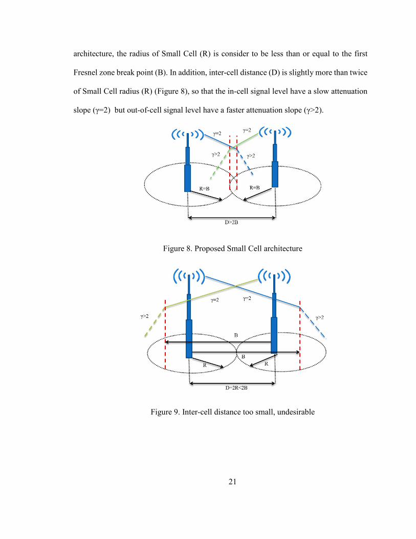
21
architecture, the radius of Small Cell (R) is consider to be less than or equal to the first
Fresnel zone break point (B). In addition, inter-cell distance (D) is slightly more than twice
of Small Cell radius (R) (Figure 8), so that the in-cell signal level have a slow attenuation
slope (γ=2) but out-of-cell signal level have a faster attenuation slope (γ>2).
Figure 8. Proposed Small Cell architecture
Figure 9. Inter-cell distance too small, undesirable

22
If two Small Cells are placed too close to each other, then the out-of-cell
interference will not attenuate fast enough, thus overall signal to interference ratio degrade
and the proper cell selection will not succeed, as shown in Figure 9.
Total out-of-cell interference can be found by adding interferences coordinated
from all neighbor cells, as shown in Figure 10. Total out-of-cell interference = ∑
(Interference coordinated from the first-tier neighbors + Interference coordinated from the
second-tier neighbors + ……+ (Interference coordinated from the kth - tier neighbors).
Figure 10. Out-of-cell interference coordinated by neighbor cells
As shown in Figure 10, each tier contains more cell than the previous ones and is
located farther away, i.e. the number of interferers increase. For instance, the first tier

23
contains six cells (yellow colored cells in Figure 10); the second tier contains 12 cells
(white colored); the third tier contains 18 cells (blue colored), and so on. The number of
cells in the kth tier is proportional to the circumference of the kth tier (2πRk), where Rk is
the average distance from the center cell (green colored). Hence, the total out-of-cell
interference can be expressed mathematically as equation (3.11)
∑∑ ====
11 )(
)2(k
k
k
k ktotalRO
ROII γ
π (3.11)
Where Ik is the total out-of-cell interference contributed by kth tier neighbor cells
and γ is the propagation path-loss slope exponent or single attenuation slope.
For example, for the path loss slope γ=4, Ik = O (
��). This means, if the path-loss
slope is steep, the interference contributed from the neighbor cells that are located far away
attenuate faster and the effect will be negligible.
However, if the path loss slope γ=2, then Ik = O (
�). This means, if the path loss
slope is too shallow, the interference contributed from the neighbor cells will be significant.
So the interference will goes up as the number of tier increases.
In the proposed Small Cell architecture, signal will attenuate faster after the cell
boundary. So, the total out of cell interference will not increase if the number of tier
increases.
3.3.3 Propagation Prediction Model for Proposed Architecture
According to Figure 7, a straight line equation can be formed with RSL0 as the
intercept at d0 is below

24
)(100
0d
dLogRSLRSL γ−= (3.12)
Where, RSL is received signal level, RSL0 is is received signal level at Fresnel
zone break point d0, and d is the distance.
Equation (3. 12) can be rewrite as below
)
10(
0
0
10 γRSLRSL
dd
−
= (3.13)
Since the cell is invariant to the propagation environment within first Fresnel zone
breakpoint and signal attenuates with attenuation slope γ=2, the path loss PL0 and received
signal level can be found by free space path loss formula as below
PL0 = 32.44 + 20 log(f) + 20 log(d0) (3.14)
RSL0 (d = d0) = ERP - PL0 (3.15)
Where, f is operating frequency band in MHz and ERP is Effective Radiated
Power in Watts. By combining equation (3.14) and (3.15), one we found
RSL0 = ERP – {32.44 + 20 log(f) + 20 log(d0)} (3.16)
Furthermore substituting equation (3.16) into (3.13), we obtain the general
propagation prediction formula is obtained
(3.17)
This
forms the basis development of the proposed Small Cell deployment.
]10
)}log(20)log(2044.32{[
0
0
10 γRSLdfERP
dd
−++−
=

25
CHAPTER 4
CELL SELECTION AND HANDOVER IN SMALL CELL NETWORKS
4.1 Introduction
The deployment of traditional cellular network (including LTE) based on the
assumption of a planned layout where a set of base-stations (Macro Cells) are deployed
with similar characteristics such as similar transmit power, antenna patterns, receiver noise
floors etc. But in case of Heterogeneous Networks, different low power nodes with
different characteristics are deployed that introduces randomness of cell deployment,
which also increases the challenges for selecting an optimum serving cell.
In case of a conventional homogeneous network, initial cell selection, cell
reselection in idle mode, and handovers are based on the highest reference signal received
power (RSRP) measured at User Equipment (UE). Although this gives the optimum
selection methodology for single-layer networks, but it does not always apply to the
Heterogeneous Networks (HetNets) where base stations can have different transmit powers
and various coverage areas such as Macro Cells, Micro Cells, Pico Cells, Femtocells, and
relays [26]. Usually, Macro Cell and Pico Cell base stations, namely MeNBs and Pico-
eNBs, differ by almost 16 dB in their downlink transmit power levels.
Small Cells are deployed within the Macro Cell to increase the network capacity
and avoid coverage holes by adapting varying nature of user traffic demand [27]. Since
Macro Cell uses higher transmitted power compared to Small Cells, UEs are more likely

26
to connect to Macro Cell even when the path loss condition between the UE and Small
Cells are better, if the cell selection is based on RSRP only. That leads the improper cell
selection and increases the probability of call drop [28]. To minimize these effects, cell-
specific handoff (HO) parameter optimization is needed to consider for Heterogeneous
Networks, unlike the same set of HO parameters (e.g., hysteresis margin, time-to-trigger,
UE velocity, etc.) for the single layer Macro network [29]. Many cell selection schemes
are proposed in [28, 30, 31, 32, 33, and 34].
4.2 Conventional Cell Selection Methods
When a UE first powers on in order to establish network attach process, it must
determine the best cell to camp on (i.e., cell selection. After connecting to the network,
Heterogeneous Networks have the mobility support that allows UE to move one cell to
another cell in idle mode (i.e., cell reselection) and also in active mode (i.e., handover). In
heterogeneous networks, two types of cell selection methods are specified. One is the
Reference Signal Received Power (RSRP)-based cell selection and the other one is
Reference Signal Received Quality (RSRQ)-based cell selection.
4.2.1 RSRP-Based Cell Selection
A cell is considered to be suitable cell if Reference Signal Received Power (RSRP)
is greater than the minimum RSRP value specified in that cell, which ranges from -144dBm
to -44dBm [22].
CellIDServing = arg max{i}{RSRPi} (4.1)
Macro Cell has larger downlink coverage due to high transmission power, but Small
Cell has small downlink coverage due to low transmission power. On the other hand, the

27
uplink coverage doesn’t change, since the transmitter is a set of the UEs. Therefore, the
optimum cell size for downlink and uplink are different and this introduces
downlink/uplink imbalance problem. According to Release8 specifications, biasing the cell
selection (i.e., Cell Range Expansion) is allowed, and the UE can then determine the best
cell by the following relationship:
CellIDServing = arg max{i}{RSRPi + biasi} (4.2)
The cell selection bias can range from 0 to 20 dB based on different propagation
environment. Since the RSRP-based cell selection only reflects the received power from
each cell and does not reflect the quality of the channel, the offloaded UE may suffer severe
interference caused by the Macro Cell if the bias is large.
4.2.2 RSRQ-Based Cell Selection
UE can also determine the best cell based on the RSRQ value (i.e., -3dB to 19.5dB
according to specification) if eNodeB is configured to do so. The RSRQ under the full load
conditions is defined by: [35]
SINR
SINR
RSSI
RSRPRSRQ
+==
1 (4.3)
Where, RSSI is received signal strength indicator, and SINR is signal-to-
interference-plus-noise ratio. Since RSRQ increases with increasing the SINR, therefore it
functions similarly as the SINR-based cell selection [30]. But RSRQ-based cell selection
allows more users offloaded to Small Cell with high SINR compared to SINR-based cell
selection. By introducing the bias, the UE selects the best cell according to the following
relationship:
CellIDServing = arg max{i}{RSRQi + biasi} (4.4)

28
4.3 Proposed Cell Selection and Hand-Off Mechanism
In the proposed cell selection method, the UE determine the best cell by the value
of the signal attenuation slope instead of RSRP/RSRQ. Referring to Figure 11, if any user
crosses the cell boundary and moves from Cell-A (Serving Cell) to Cell-B (Candidate
Cell), the user will experience a rapid attenuation of received signal strength due to a large
attenuation slope. As a result prompt hand-off will take place to Cell-B, since the downlink
signal from Cell-B experienced lower attenuation slope (γ=2).
Figure 11. Proposed hand-off scenario
When the eNodeB analyses the UE measurement report, it can get information
about received signal strength based on location (equation 4.5). By Tracking Area Indicator
(TAI), the eNodeB can identify the UE location and can get the value of attenuation slope
or path loss slope (γ) provided by the propagation model specified in that eNodeB.
RSL(x, y, z) ∞ d-γ (x, y, z) (4.5)

29
Where, RSL(x, y, z) represents the received signal level as a function location, d(x,
y, z) is the distance with respect to location, and γ is the attenuation factor provided by the
propagation prediction model.
4.4 Performance Analysis of Proposed Hand-Off Mechanism
Small Cells are deployed within the Macro Cell coverage to increase the network
capacity, but if we consider dense deployment of Small Cell, traffic offloading to Small
Cell becomes a critical issue, as explained in the following two scenarios:
4.4.1 Scenario-1: When Small Cell Very Close to Macro Cell
Referring to Figure 12, the user is served by Small Cell but it will get stronger signal
from Macro Cell, since Macro Cell has high transmission power. If the cell selection is
based on RSRP/RSRQ, the user is likely to connect with Macro Cell, but in the proposed
plan the user can be served by Small Cell due to lower attenuation slope (γ=2).
Figure 12. Proposed hand-off scenario-1

30
4.4.2 Scenario-2: When Two Small Cells Are Very Close
In Figure 13, the user is served by Small Cell-A but it will also get a strong signal
from neighbor Small Cell-B. If the cell selection is based on RSRP/RSRQ, the user will
experience lack of dominant cell and the number of handover signaling increases to find
the dominant cell. This problem is solved by the proposed plan, since the out-cell
interference attenuates fast due to large attenuation slope and the user connected with
serving cell without interruption.
Figure 13. Proposed hand-off scenario-2
In this chapter, conventional cell selection methods for Heterogeneous Networks
are studied and proposed a new cell selection method based on signal attenuation slope. It
is found that the proposed cell selection method allows seamless offloading the traffic
between Macro Cell and Small Cell. Thus, dense Small Cell deployment is possible to
hence the network capacity without degrading the network quality.

31
CHAPTER 5
COVERAGE AND CAPACITY DIMENSIONING
5.1 Coverage Planning
The coverage estimation is used to determine the coverage area of each base station.
Coverage estimation calculates the area where base station can be heard by the users
(receivers). It gives the maximum area that can be covered by a base station. But it is not
necessary that an acceptable connection (e.g. a voice call) between the base station and
receiver can be established in coverage area [36]. However, base station can be detected
by the receiver in coverage area.
Coverage planning includes Radio Link Budget (RLB) and Coverage analysis [37].
For the planning of any Radio Access Networks (RAN) begins with a RLB. RLB comprises
the accounting of all gains and losses from the transmitter end (base station site), through
the medium (i.e. free space, cable, waveguide, fiber, etc.) to the receiver end (mobile
station) in a telecommunication system [38]. The maximum allowed receive signal level at
the mobile station to the base station is estimated which allows to calculate the maximum
path loss allows to get maximum cell range that leads to estimate a suitable propagation
model. According to the cell range, it allows to estimate the total number of base station
sites required to cover a required geographical area.

32
5.1.1 Radio Link Budget
Since operators are rightfully focused on the service quality of a system, radio
network coverage becomes an important part of the service quality of a system. The main
purpose of radio network planning is to keep a balanced coverage, capacity, system quality,
and total cost so none of these can be considered in isolation.
The purpose of Radio Link Budge (RLB) can be sort out as follows [36]:
1. Calculate such a factor that can solely describe building penetration loss, feeder
loss, transmitting antenna gain, receiver antenna gain, and the interferences.
2. Calculate the margin of the radio link to find out all the related gains and losses
that can affect the whole cell coverage.
3. Based on eNodeB transmit power allocation and the maximum transmit power of
the terminal, estimate the maximum link loss of a radio link.
4. Whenever estimate the maximum link loss of a radio link allowed under certain
propagation model, coverage radius of a base station can be obtained. Then this
radius can be used for subsequent designs.
During radio network planning designer needs to consider various factor that will
affect the coverage radius of a cell and the total number of base stations required to cover
any particular area. The key affecting parameters are groups as followings:
1. Propagation related parameters, such as the penetration loss, feeder loss, body loss,
and background noise.
2. Equipment related parameters, such as transmit power, receiver sensitivity, and
antenna gain.

33
3. LTE specific parameters, such as Multiple Input Multiple Output (MIMO) gain,
power boosting gain, edge coverage rate, repeat coding gain, interference margin,
and fast fading margin.
4. System reliability parameters, such as slow fading margin.
5. Specific features that will affect the final path gain.
Note is that the link budget is based on only theories, and it cannot ensure the
system capacity and coverage reliability of the actual network. The actual coverage target
and requirements also vary with different network requirements [39, 40]. Consequences,
the link budget result varies greatly in reality, and depending on the different input
parameters that is varied with situation and requirements. Therefore designer’s need to
discuss with the operator to estimate the value of each input parameter in the link budget
to estimate a link budget that will reflects the requirement of a particular networks.
Link budget also assumes some parameters, such as a uniform landform, simple
terrain, ideal site locations, and even subscribers distribution. The simulation covers
detailed landform distribution, actual site location, terrain serves only as theoretical
calculation result. This calculated coverage radius is further used as reference for simulated
site distribution. For a given coverage area, the number of base stations needed depends on
the simulation results.
Radio Link Budget model for uplink (UE to eNodeB) and downlink (eNodeB to
UE) are shown in Figure 14 and 15.

34
Figure 14. Downlink Radio Link Budget Model
Figure 15. Uplink Radio Link Budget Model

35
The basic Radio Link Budget equation for LTE can be written as follows (in units
of dB) [36, 25]
PRX = PTX + GTX + GRX – LTX – LRX + PM - LP (5.1)
Where, the PRX is the received power (dBm). PTX is the transmitted output power
(dBm). GTX and GRX is transmitter and receiver antenna gain (dBm), respectively. LTX
and LRX are the cable and other losses on the transmitter and receiver side (dB)
respectively. PM is the planning margin and LP is the path loss between transmitter and
receiver end.
The maximum available transmission power is equally divided over the cell
bandwidth; the average received power (AveRxPowerDL) in the bandwidth allocated to
the user is derived as follows [41]:
LinkLossDL
andwidthAllocatedB
dthCellBandwi
PowerMaxNodeBTx
LinkLossDL
AveTxPowerDLAveRxPower ×==
(5.2)
Where,
AveTxPower = Average transmitted power (W)
LinkLossDL = Total Link Loss in Downlink (W)
MaxNodeBTxPower = Maximum Power transmitted from eNodeB (W)
CellBandwidth = Allocated bandwidth of LTE network cell (MHz)
Allocated bandwidth= Bandwidth of channel over which the signal is transmitted
In LTE network MaxNodeBTxPower depends on the cell bandwidth and the range
is from 1.25MHz to 20MHz. Specifically, MaxNodeBTxPower is 20 Watt (43 dBm) up to
5 MHz and 40 Watt (46 dBm) above this limits [42].

36
The average received power (AveRxPowerUL) can be written with assuming no
power control as follows:
LinkLossUL
erMaxUETxPowULAveRxPower = (5.3)
Where,
MaxUETxPower = Max transmission power of user equipment (UE in Watt)
LinkLossUL = Total link loss in uplink (W)
The max transmission power of user equipment can be either 0.125 W or 0.25 W
(21 dBm or 24 dBm) [42]. Total link loss in uplink includes the path loss which is distance
dependent and all other related gains and losses at the transmitter and the receiver. In case
of uplink, gains include antenna gains and amplification gains (e.g., Mast Head Amplifier
in UL direction). And also, the losses include body loss, cable loss and Mast Head
Amplifier noise figure at the eNodeB and finally some margins and other losses needed to
take into account are shadow fading and indoor penetration loss. Therefore, link loss can
be defined as:
sOtherLosseTxLossesRxLossesPathLoss
sTxGainRxGainsLinkloss
××××= (5.4)
The received noise power (RxNoise) can defined as follows:
RxNoise = ThermalNoise × ReceiverNoiseFigure (5.5)
= (ThermalNoiseDensity × AllocatedBandwidth) × ReceiverNoiseFigure
Where,
ThermalNoise = Thermal Noise (W)
ReceiverNoiseFigure = Receiver Noise (W)
Thermal Noise Density = -174 dBm

37
Orthogonal Frequency-Division Multiple Access (OFDMA) is used in the
downlink (DL) and if assuming the appropriate length of cyclic prefix, then we can assume
that there is no own cell interference (Own Cell Interference is Zero). But there will be
Other Cell Interference which is the total average power received from other cells in the
allocated bandwidth. Similarly, in the UL direction the Interference (also called Noise
Rise) is the power received from terminals transmitting on the same frequency in the
neighboring cells (Other Cell Interference) [43].
Above set of equations lay the basis for calculation of RLB equation for maximum
allowed path loss. Here, we get the result
∑ ≠+
=+
=+
=
ownkN
kLinkLoss
kAveTxPwr
ownLinkLoss
ownAveTxPwr
Nother
ownAveRxPwr
N
ownAveRxPwrSINR
)(
)()(
)(
)(1
)(
1
)( (5.6)
∑ ≠××+
=
mkureRxNoiseFigseDensityThermalNoi
MaxTxPwr
CellBW
kLinkLoss
ownLinkLoss
)(
1)(
1
(5.7)
LTE radio network requirements are as follows:
SINR ≥ Required SINR (5.8)
Now putting this in the above equation we get the following form of Path Loss:
∑ ≠×+
≤
ownkquiredSINRnentNoiseCompo
kPathLoss
ownPathLoss
Re))(
1(
1)(
(5.9)
a) Interference (i): To include the effect of interference, Other-to-own cell
interference for DL can be written as follows

38
∑ ≠=
ownk kPathLoss
ownPathLossi
)(
)( (5.10)
Rewriting this equation according to RequiredSINR requirements as follows
quiredSINRownPathLossnentNoiseCompoi
Re)(
1 ≤×+
(5.11)
Thus, the maximum path loss LTE can write as follows:
quiredSINRnentNoiseCompo
quiredSINRsMaxPathLosisMaxPathLos
Re
Re)(1
××−= (5.12)
Therefore it is found that all the conventional RLB components are in the Noise
Component. Noise component is the inverse of the conventional path loss [43, 44].
In case of uplink the issues of interference is dealt as interference margin which can
be calculated using the following equation:
Interference MarginSINR
SNR= (5.13)
Where,
SNR = Signal to noise ration
SINR = signal-to-interference-plus-noise ratio
b) Spectral efficiency: Whenever cell edge of a particular cell is defined
according to required throughput, the corresponding spectral efficiency has to be derived.
According to Alpha-Shannon formula Spectral efficiency of a radio network can be written
as follows [11]:
)101(log 102
SNR
ficiencySpectralEf +×=α (5.14)

39
The maximum capacity of the LTE radio network cannot be obtained due to the
following factors:
1. Limited coding block length
2. Frequency selective fading across the transmission bandwidth
3. Non-avoidable system overhead
4. Implementation margins ( channel estimation, CQI)
From above equation there are two factors that affect the Shannon formula to LTE
radio link is the following:
1. Bandwidth efficiency factor (α)
2. SNR efficiency factor, denominated Impact Factor
So, the modified Alpha- Shannon Formula can be written as:
)101(log Im102
pactFactor
SNR
ficiencySpectralEf ×+×=α (5.15)
c) Required SINR: For a given cell throughput cell edge of a particular cell is
solely depends on the Required SINR value. That’s why required SINR becomes the main
performance indicator for LTE Radio network. Required SINR is depends on the following
two factors [45]:
1. Modulation and Coding Schemes (MCS)
2. Propagation Channel Model
As higher the modulation and coding schemes used, higher the required SINR is
required. For example using Quadrature Phase Shift Keying (QPSK) has a lower required
SINR compared to 16QAM (quadrature amplitude modulation).

40
Maximum allowed path loss of a LTE Radio Network is calculated according to
the following condition:
SINR ≥ Required SINR (5.16)
SINR = (AveRxPower)/(Interference+RxNoise) (5.17)
Where, SINR is Signal to Interference and Noise Ratio. AveRxPower is average
received power (W). Interference is interference power (W) which comprises the own
channel interference (i.e., Power due to own cell interference) and Other Cell Interference
(i.e., power received for neighboring cells). RxNoise is the receiver noise power which
includes thermal noise and receiver noise figure.
5.1.2 Coverage Analysis
Coverage analysis gives the estimation of the resources needed to provide service
in the deployment area with specific system requirements. Since the LTE system allow
providing high quality of service and high capacity, estimating inaccurate coverage has
severe impact on the system performance. Over estimating the coverage area causes
received signal level at a distance from base station weaker than the minimum required
threshold [46, 47]. And even under estimating the coverage area results in coverage area
overlap, which causes interferences and degrade the system performance. Thus, accurate
estimation of coverage is the key to design a good radio network. In this section, the cell
radius of a particular LTE sector is calculated based on the propagation environment.
When the received signal is measured over the distance of a few tens of wavelength,
the receive signal level shows rapid and deep fluctuations about the local mean with the
movement of user equipment (e.g., mobile terminal). It is difficult to describe by

41
mathematical equations because the Radio Frequency (RF) propagate through transmitter
end to receiver end depends on lots of factor such as, proximity to buildings, the actual
terrain, antenna heights, topology, morphology, Etc. That’s why the selection of a suitable
RF propagation model for LTE radio network is of great importance [48, 49].
Figure 16. Receive Signal Level at a distance d from the base station
RF propagation model describes the behavior of the transmitted signal while it is
transmitted from transmitter end towards the receiver end, as described in section 5.1.3. It
gives the relation between transmitter and receiver end and from this relation designers can
get an idea about the maximum allowed path loss between transmitter and receiver end and
can estimate the maximum cell range, shown in Figure 16.
As shown in Figure 14 and 15, designers can easily estimate the transmitted output
power, transmitter and receiver antenna gains, the cable and other losses on the transmitter
and receiver sides but the designers cannot predict path loss between the medium of
transmitter and receiver end. The path loss criteria are solely depends on the RF

42
propagation environment (urban, rural, dense urban, suburban, open, forest, sea etc.),
operating frequency, atmospheric conditions, indoor/outdoor & the distance between
transmitter end & receiver end.
Note that empirical formulas do not estimate the actual coverage needed for
designing a network. Several computer based prediction tools [48] model that uses the
physical phenomenon of RF propagation using terrain and clutter (land use) data. To get
the accuracy of coverage estimation using these tools depends on the accuracy and
resolution of the available data. Even when accurate and high resolution clutter data is
available, the effect of the clutter on the RF propagation may different due the different of
areas. For example, if the clutter data classifies an area as dense urban considering, average
building height, there is still an ambiguity found about the density of the buildings in the
area and also RF propagation depends on the materials used to construct the buildings [50].
Also the propagation characteristics in an area classified as dense urban in one country will
never be equal in another country. That’s why designers always need lots of simulation
before deploying any network and it saves lots of money of an operator.
5.1.3 Okumura-Hata Propagation Prediction Model
The most widely used radio frequency propagation model for predicting the
behavior of cellular propagation is the Hata Model for Urban Areas, also known as the
Okumura-Hata model for being a developed version of the Okumura Model. This model
incorporates the effects of diffraction, reflection and scattering caused by different city
structures.

43
Okumura model for urban was the first model and used as the base for the others.
According to Okumura-Hata propagation model there are four different types of
propagation environment and considering each propagation environment there is a
propagation model [25].
1. Dense Urban Model
2. Urban Model
3. Sub-Urban Model
4. Rural Model
The traditional Okumura-Hata model for path loss formula is given by [25]
Lp(dB)=C0+C1+C2 log(FMHZ)-13.82 log(Hb)-a(Hm)
+[44.9-6.55 log(Hb)] log(dKm) (5.18)
Where C0, C1 and C2 are constants and are given
C0 = 0 for Urban
= 3 dB for Dense Urban
C1= 69.55 for 150 MHz to 1000 MHZ
= 46.30 for 1500 MHz to 2000 MHz
C2 = 26.16 for 160 MHz to 1000 MHz
= 33.90 for 1600 MHz to 2000 MHz
f = Frequency in MHz
d = Distance (cell radius) in Km
Hb = Base station antenna height in meters
for Urban,
a(Hm) ={1.1 log (FMHz) - 0.7}Hm – {1.56 log (FMHz) – 0.8} (5.19)

44
for Dense Urban,
a(Hm) = 3.2[log{11.75 Hm }]2 – 4.97 (5.20)
Hm = Mobile Antenna height in meters
From equation (5.18) we can find the cell radius
dKm= anti log [{Lp(dB)-C0-C1-C2 log(FMHZ)+13.82 log(Hb)
+ a(Hm)}/ {44.9-6.55 log(Hb)}] (5.21)
Using this cell radius the cell coverage area of a particular cell can be calculated
and it is depended on the site configuration. Designers consider hexagonal cell for design
purpose although the deployment area is irregular in shape. For hexagonal cell models, cell
coverage for omni-directional sites, Bi-sector sites, and tri-sector sites can be calculated by
equations 5.22, 5.23, and 5.24, respectively.
Site coverage area (Omni-directional site) = 2.6 * CellRadius2 (5.22)
Site Coverage area (Bi-sector site) = 1.3 * 2.6 * CellRadius2 (5.23)
Site Coverage area (Tri-Sector site)= 1.95 * 2.6 * CellRadius2 (5.24)
5.2 Capacity Planning
Capacity planning is crucial to estimate the resources needed for supporting a
specified offered traffic with a certain level of QoS (e.g. throughput or blocking
probability) [45]. Theoretical capacity of the network is limited by the number of cells
installed in the network. In short the capacity dimensioning can be described by the
flowchart, shown in Figure 17. Total number of sites need to cover a geographic area can
be found after calculating the number of sites based on coverage and number of sites based
on capacity.

45
Figure 17. Capacity Dimensioning
5.2.1 Number of Sites due to Coverage
Total number of sites needed to cover a deployment area can be calculated as
follows:
Total Number of SitesgeAreaSiteCovera
AreaDeployment= (5.25)
Where, Deployment Area is the planned area needed to cover by network and Site
Coverage Area can be calculated from the radio link budget, the propagation model and
the type of cell site (discussed in section 5.1.3).

46
5.2.2 Number of Sites due to Capacity
The first step is to find the subscriber density. Subscriber density for a particular
operator depends on the population density of the planned area, mobile phone
penetration, and operator market share.
The second step is to find the subscriber’s data usage requirement. The main
purpose of the traffic model is to describe the behavior of the average subscriber during
the most loaded day period (e.g., the Busy Hour time). Different data types are given
below
a). Voice: Calculate the Erlang per subscriber for voice call during busy hour of
the network
b). Video Call: Calculate the Erlang per subscriber for video call during busy
hour of the network
c). NRT Data: Calculate the average throughput (kbps) needed per subscriber
during busy hour of the network and find the target bit rates.
The third step is to calculate the total offered traffic. Total offered traffic can be
calculated after finding the total number of subscriber and the average data rates per
subscriber during busy hour time. Let’s consider an example. In this example, the total
number of subscriber is known as P and the average data volume per subscriber per busy
hour (BH) found is N MByte. Now, the average data rate per subscriber can be calculated
as
Average date rate per subscriber = Average Data Volume per subscriber per BH (bit)/3600s
(5.26)
The total offered traffic can be calculated as

47
Total offered traffic=Number of Subscriber * Average Data Rate per subscriber (5.27)
The next step is to find out the site capacity and it can be calculated as
Site capacity = Cell Capacity * Number of Cells per site (5.28)
Where, cell capacity is defined as the overall cell throughput [51].
The last step is to find the capacity base site count and it can be calculated as
Sites due to capacity = Roundup (Total Offered Traffic/Site Capacity) (5.29)
5.3 Factors Affecting the Cell Capacity
Based on the fundamental limit given by the Shannon’s capacity formula, the
maximum number of bit/sec/m2 is given by the following equation
))(
)((2
NI
PnwLogC
+=
λλλ (5.30)
Where,
λ = Base station density
n = No. of signaling dimensions: MIMO “multiplexing” gain
W = Bandwidth
I(λ) = Interference Power
P(λ) = Received signal power, and
N = Noise signal power
The cell capacity can be optimized based by optimizing the different factors in
equation 5.30. There are several factors that can impact on network capacity. The major
factors are discussed below
48
5.3.1 Cell Range (Pathloss)
Path loss condition is greatly varies with different geographic area and it has great
impact on inter site distance. Besides, the inter site distance (ISD) impact on network
capacity because as the ISD goes up the number of site can deploy in an area is going down,
so the total network capacity will goes down as well. So, the base station density can be
optimized by minimizing the ISD. In real planning scenarios, ISD obtained from radio link
budget is not equal to the ISD obtained in the radio network simulation (e.g., ATOLL).
Therefore additional interpolation is required to adapt the results from the radio link
budget.
5.3.2 Channel Bandwidth
Due to the maximum frequency diversity gain, the best capacity performance can
be achieved with the wider channel bandwidth. The available maximum bandwidth in case
of LTE is 20MHz. So next generation cellular networks (e.g., 5G) looking for wider
bandwidth called millimeter wave wireless communications (i.e., 3- 300 GHz). According
to equation 5.30, linear capacity gain is possible by adding more bandwidth but it requires
expensive resources.
5.3.3 Cell Load
Full resource utilization means the 100% cell load. It will be the worst case in terms
of interference, shown in the following Figure 18. The center black color cell is fully loaded
all the time is the victim cell for which the overall cell throughput is measured. The
surrounding cells are not fully loaded and impact the victim cell by inter-cell interference
which depends on the neighbor cell load condition. When the neighbor cell load decrease

49
the victim cell throughput is increased. So, the cell load condition can have great impact
on cell capacity.
Figure 18. Impact of cell load
In this chapter describes the coverage and capacity dimensioning of Heterogeneous
Networks. The different factors that affect the coverage and capacity planning is also
outlined. In the next chapter shows different interference scenarios of Heterogeneous
Networks and the interference coordination techniques.

50
CHAPTER 6
INTERFERENCE IN SMALL CELL NETWORKS
6.1 Interference Challenge
In general, interference occurs when two or more devices are transmitting close
each other (i.e., the devices are physically near each other and transmitting with same or
nearby frequencies or channels). Since Heterogeneous Networks is not handled by
carefully network and frequency planning, the interference issue is more challenging in
Heterogeneous Networks than homogeneous networks. Intra-tier interference occurs in
heterogeneous networks like as homogeneous networks, where a Macro Cell interfere with
neighbor Macro Cells and a Small Cell (e.g., Femtocell) interferes with neighbor Small
Cells. However, the most severe interference occurs in the cross-tire interference; where
Macro Cell interfere with Small Cells or a Small Cell interfere with Macro Cells [52].
In heterogeneous networks different type of cells can co-exist and the cells differ
in their own characteristics. So the uses of different backhaul links introduces more
challenges in interference coordination schemes, where each link supports different
bandwidth and delay constraints (e.g., Pico Cells and relays use X2 interface whereas
Femtocells use xDSL for exchanging signals) [53]. The main reasons that cause
interferences in heterogeneous networks are discussed below:

51
6.1.1 Power Difference
In heterogeneous networks, Macro Cells and Small Cells are differ strongly in
downlink transmit power that leads to a particular interference challenge (i.e., downlink
uplink imbalance problem), shown in (Fig. 19). Since the Macro Cells transmit in high
transmission power (e.g., 43dBm), the downlink coverage of Macro Cells are much higher
than of Small Cells. On the other hand, the uplink coverage does not affect by the difference
in downlink transmit power, since the transmitters (i.e., UE or mobile users) are same for
the Macro Cells and Small Cells [32]. So, the optimum cell will be different for downlink
and uplink connection. As a result, when UE is connected to one cell (serving cell) and
come closer to another cell (non-serving cell or neighbor cell), it will receive high power
from the non-serving cell interfering it’s downlink. Several interference scenarios are
discussed in section 5.2.
Figure 19. Problem caused by difference in power between Macro and Small Cells

52
6.1.2 Unplanned Deployment
In heterogeneous networks, Small Cells can be deployed and monitored by the
subscriber which is not a planned deployment [54]. The networks operator doesn’t have
any control on them that causes load-neighbor effect. Thus, network planning and
optimization becomes inefficient that leads to decentralize the interference management
schemes, where the interference management schemes are applied each cell independently
(e.g., Self Organizing Networks) by using the local information to achieve efficient gain
for the network.
6.1.3 Closed Subscriber Group (CSG) Access
In heterogeneous networks, some Small Cells (e.g., Femtocells) can be configured
as closed subscriber group access, where network access is restricted by the owners and
the approved users can only get the access of the networks [55]. As a result, when any user
comes near a closed subscriber group access node and cannot get access due to outside
users, it will suffer cross-tier interference. In this case, the victim users starts to transmit at
higher power to compensate the path loss for the it’s far away serving Macro Cell that leads
to jamming the unlink of the nearby closed subscriber group access node [29].
6.2 Small Cell Interference Scenarios
A set of interference scenarios for the deployment of Small Cell is discussed in
this section [6, 8, 22]. In the following analysis, SC UE represents user served by the
Small Cell, Macro UE represents, user served by the Macro Cell, and the red dotted line
represents interfering signal.

53
6.2.1 Macro Cell Downlink to the Small Cell UE Interference (Traffic Channel)
The first interference mechanism to consider is where the Small Cell users
interfered by the downlink signal of Macro Cell, shown in (Fig. 20). In this scenario, the
Small Cell and the Macro Cell use the same spectrum for serving their related UEs. If the
signal of the Macro Cell is strong at the location of the SC UE, the SC UE will be interfered
by the Macro Cell that serves its UEs by the same radio resources.
Figure 20. Macro Cell Downlink to the Small Cell UE Interference
6.2.2 Macro Cell UE Uplink to the Small Cell Interference (Traffic Channel)
Figure 21. Macro Cell UE Uplink to the Small Cell Interference

54
The second interference mechanism to consider is where the Macro Cell user
interfered by the uplink signal of Small Cell. In this scenario, one UE is served by the
Macro Cell is close to the SC which is remote from the Macro Cell. Since the macro UE is
remote from its serving Macro Cell it will transmit high power signal to reach it. However
this signal might reach the SC with high enough power to interfere with the reception of
the uplink signal arriving from the SC UE, shown in (Fig.21).
6.2.3 Small Cell Downlink to the Macro Cell UE Interference
According to (Fig.22) a Macro UE is served by a Macro Cell, but when it comes
closer to the Small Cell, the Macro UE is interfered by the Small Cell downlink signal.
Figure 22. Small Cell Downlink to the Macro Cell UE Interference
If the downlink signal of the Small Cell provides better service than the Macro Cell,
it may trigger the handoff request to the Small Cell. In this case, if the Small Cell is
configured a closed subscriber group policy, this handoff request will not successful and
the victim Macro UE will suffer severe disturbances without additional interference
mitigation mechanism.

55
6.2.4 Small Cell UE Uplink to the Macro Cell Interference
Here is another interference scenario, where Macro UE is interfered by the uplink
signal of SC UE, shown in (Fig.23). In the following this scenario, a faraway Macro UE is
served by the Macro Cell and receives its uplink signal. Besides, a SC UE, served by the
Small Cell transmits high enough power to interfere with the reception of the uplink signal
arriving from Macro UE. This scenario can be more obvious in the following example
(Fig.24)
Figure 23. Small Cell UE Uplink to the Macro Cell Interference
Figure 24. Small Cell UE Uplink to the Macro Cell Interference (Example)

56
Let’s a SC UE is located on a top floor with a line of sight to the Macro Cell and a
Macro UE is located far away from the Macro Cell and its communication path to the
Macro Cell antenna is obscured by buildings or by other obstructions. It is assumed that
both UE is transmitting at maximum power level. Since the maximum power levels of the
UEs are usually identical, Macro Cell might receive significantly higher uplink signal from
SC UE compared to Macro UE and therefore Macro UE will suffer severe interference
without additional interference mechanism technique.
6.2.5 Small Cell Downlink to the nearby Small Cell UE Interference
This interference mechanism is considered for indoor scenario like multistoried
buildings, where one Small Cell users interfered by the downlink signal of neighbor Small
Cells. In the following example shown in (Fig.25), SC UE1 is served by the Small
Cell1.When SC UE1 comes closer to Small Cell 2, it will still serve by the Small Cell 1
but it might receive strong interfering downlink signal from Small Cell 2. In this case, SC
UE1 will trigger handoff to Small Cell 2 but if Small Cell 2 is configured closed subscriber
group then this handoff request will not successful. Therefore this kind of system will
perform poorly without any additional interference mechanism technique.
Figure 25. Small Cell downlink to the nearby Small Cell UE Interference

57
6.2.6 Small Cell UE Uplink to the nearby Small Cell Interference
This is the second interference mechanism considered for indoor scenario like
multistoried buildings, where one Small Cell users interferes the uplink signal of another
Small Cell users.
Figure 26. Small Cell UE Uplink to the nearby Small Cell Interference
According to (Fig.26), SC UE2 is served by the Small Cell 2 and SC UE1 is served
by the Small Cell1. When SC UE2 move away from Small Cell 2 and the SC UE1 come
closer to Small Cell 2, it might interfere the uplink signal of SC UE2. It can happen when
the path loss condition between Small Cell 1 and SC UE1 becomes high, SC UE1 starts
transmitting with high power. Thus a significant interference might occur. Again, without
an additional interference mitigation mechanism this kind of system cannot perform well.
6.3 Interference Coordination in Heterogeneous Networks
In 3GPP LTE Release 10 introduces enhanced inter-cell interference coordination
(eICIC) mechanism to deal with the interference issues in Heterogeneous Networks, and
minimize interference on traffic and control channel. The techniques can be group into
frequency domain techniques, time domain techniques, and power control based solution.
All the techniques are discussed in this section.

58
6.3.1 Frequency Domain Techniques
In inter-cell interference coordination (ICIC) technique, system spectrums are
allocated for interference cells by partitioning. Carrier Aggregation (CA) is introduced in
3GPP LTE Release 10 that brings additional opportunities for frequency domain
interference mitigation [54]. It allows users to transmit/receive simultaneously on multiple
carriers. In case of CA-based ICIC techniques, CA creates protected component carrier
(CC) for each users in victim layers, where the data is received on scheduled cross-carrier
components, shown in (Fig.27) [55].
Figure 27. Frequency domain eICIC Techniques
For the deployment of Macro-Pico scenario, the macro node is the aggressive node,
whereas the Pico users are the victim users. After applying the CA-based ICIC techniques,
Macro Cell mute it’s control channel transmission on one carrier (CC1) and it schedules
users on both carriers by using the control region from the second carrier (CC 2). Thus
there will be no interference in the control region for the cell edge users. In case of Pico
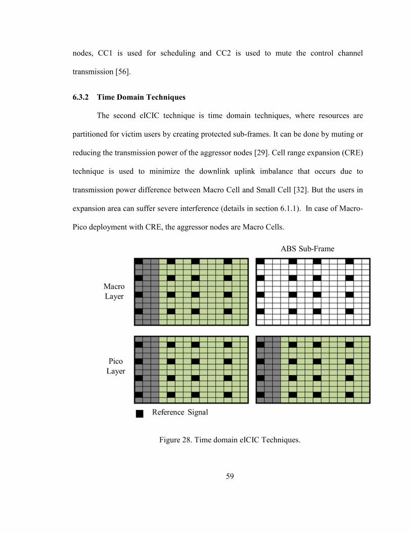
59
nodes, CC1 is used for scheduling and CC2 is used to mute the control channel
transmission [56].
6.3.2 Time Domain Techniques
The second eICIC technique is time domain techniques, where resources are
partitioned for victim users by creating protected sub-frames. It can be done by muting or
reducing the transmission power of the aggressor nodes [29]. Cell range expansion (CRE)
technique is used to minimize the downlink uplink imbalance that occurs due to
transmission power difference between Macro Cell and Small Cell [32]. But the users in
expansion area can suffer severe interference (details in section 6.1.1). In case of Macro-
Pico deployment with CRE, the aggressor nodes are Macro Cells.
Figure 28. Time domain eICIC Techniques.

60
In time domain eICIC, ABS (almost blank sub frames) is used for the Macro Cell
where no control or data signals is transmitted except reference signals. All the users in
extension area are scheduled within the sub-frames overlapping with ABS of the Macro
Cells, which mitigates the cross-tier interference significantly.
6.3.3 Power Control Based Solution
Power control based eICIC technique is used to mitigate the interference for the
Macro-Femto deployments scenario. After applying this technique, Femto cell can
automatically adapt its transmission power and users connected to them by observing the
interference conditions, deployments, and cell loads, etc. It is noted that, power reduction
is not applied in the Macro Cell because it will reduce the Macro Cell coverage [29].
In this chapter describes mobility management challenges in Small Cell networks
and shows different interference scenarios. This chapter also shows possible interference
coordination mechanism for Small Cell networks. The following chapter shows
simulation and results.

61
CHAPTER 7
SIMULATION AND RESULT
7.1 Calculating Small Cell Radius
In the proposed Small Cell architecture, the radius of Small Cell is less than the
first Fresnel zone break point and can be calculated by equation (3.10). According to this
equation, the Fresnel zone break point varies with different antenna heights and operating
frequency band. The first simulation result shows the different values of Small Cell radius
(e.g., for indoor d=50m and for outdoor d=294m) by varying the transmitting antenna
height, shown in (Fig. 29). In this simulation, receiver antenna height is considered as 1.5m,
and operating frequency band is 2100MHz.
Figure 29. Fresnel zone break point varies with Tx height (F=2100MHz, h1=1.5m)

62
The second simulation result shows the different values of Small Cell radius (e.g.,
for f=2100MHz, d=840m and for f=3.5GHz, d=1400) by varying the operating frequency
band, shown in (Fig. 30). In this simulation, receiver antenna height is considered as 1.5m
and transmitting antenna height as 20m (for outdoor scenario).
Figure 30. Fresnel zone break point varies with TX Height (h1=1.5m, h2=20M)
The third simulation result shows the different values of Small Cell radius (e.g., for
f=2100MHz, d=126m and for f=3.5GHz, d=210) by varying the operating frequency band,
shown in Figure 31. In this simulation, receiver antenna height is considered as 1.5m and
transmitting antenna height as 3m (for indoor scenario).
Based on Figure 29, 30, and 31, it is obvious that for different deployment
environments (e.g., indoor or outdoor), the service provider can optimize the Small Cell
radius by adjusting the transmit antenna height with any specific operating frequency band.

63
Figure 31. Fresnel zone break point varies with Tx height (h1=1.5m, h2=20M)
7.2 Multipath Effect in Proposed plan
This simulation result shows how the multipath signal can affect the received signal
level over a distance. For multipath effect analysis the following simulation parameters
listed in Table 2.
Table 2. Simulation parameter for multipath effect in proposed plan
Cell Type Transmitter Height
Receiver Height
Operating Frequency
RSL (dBm)
Indoor 3m 1.5m 2100MHz -70dBm
Outdoor 6m 1.5m 2100MHz -70dBm
It is found that the Small Cell is insensitive to the propagation environment with
ERP=10.98mW and the corresponding cell radius is 126m (indoor cell Figure 32). But
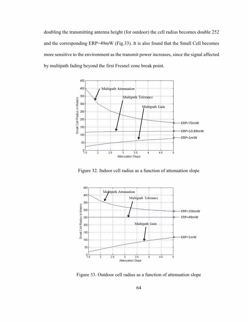
64
doubling the transmitting antenna height (for outdoor) the cell radius becomes double 252
and the corresponding ERP=49mW (Fig.33). It is also found that the Small Cell becomes
more sensitive to the environment as the transmit power increases, since the signal affected
by multipath fading beyond the first Fresnel zone break point.
Figure 32. Indoor cell radius as a function of attenuation slope
Figure 33. Outdoor cell radius as a function of attenuation slope

65
When the transmit power is too small, it introduces the waveguide effect
(constructive interference), where the reflected and diffracted components are<90 degree
out of phase and strong composite signal forms by multiple reflections. The attenuation
slope within this condition is less than 2, which means the propagation environment is
better than free space.
7.3 Path Profile Analysis
Path profile analysis shows how the signal decays over a distance from base station.
The cell site parameters for the path profile analysis are listed in Table 3.
Table 3. Simulation Parameters for Path Profile Analysis in ATOLL
Cell Type Transmitter height
Operating Frequency Transmit Power (dBm)
Macro Cell 35m 2100MHz 43Bm
Small Cell 20m 2100MHz 30 dBm
It is found that the radius of Fresnel zone is smaller closer to Macro Cell ( shown
in Figure 34) but the Fresnel zone radius increases at the cell boundary (shown in Figure
35) due to the signal affected by multipath signal beyond the Fresnel zone breakpoint. As
the radius of Fresnel zone increases it becomes more susceptible to shadowing or affected
by multipath signal. But in case of Small Cell (shown in Figure 36), the radius of small
remains within the first Fresnel zone break point and the transmitted signal is invariant to
propagation environment. Since the radius of Small Cell is within a Km, most of the area
in dense urban or urban can be covered by Small Cell networks where user will get
advantage of line of sight communication. If the users remains within line of sight
communication, it can reduce the transmission power and enhance the batter life.

66
Figure 34. Path profile analysis scenario-1 for Macro Cell.
Figure 35. Path profile analysis scenario -2 for Macro Cell
Figure 36. Path profile analysis for Small Cell

67
7.4 Coverage Analysis of Heterogeneous Networks
Coverage analysis shows how a particular serving area is covered by a network and
the analysis of received signal level in that area. After finding the Small Cell radius at
2100MHz for outdoor deployment scenario, seven Small Cell clusters are deployed within
and outside of the macro network. The coverage footprints are analyzed for both scenario,
Macro Cell only scenario, and with Small Cells by radio network planning tools called
ATOLL, shown in Figure 37 and 38. The design consideration and simulation results are
shown in below
Table 4. Cell Site Parameters.
Cell Type Antenna Height
Transmit Power
Cell Radius
Number of UE Cluster Size
Macro Cell 35m 43dBm 5Km 35 UE per Sector 7
Small Cell 20m 30dBm 840m 10 UE per Cell 4
Figure 37. Heterogeneous Networks coverage for Macro only deployment.

68
In Figure 37 and 38, the different color shows the different signal level. For
example, the best signal level shows by red color which is -70dBm and the worst signal is
represented by blue which is -105dBm. The received signal is considered as good, if the
value is more than -90dBm.In this simulation the area is covered by good quality signal
and the cell sites coverage areas are overlapped so that there is no coverage holes in the
service area.
Figure 38. Heterogeneous Network coverage with Small Cell deployment
In figure 37 shows the Heterogeneous Networks coverage considering macro cells
only and the figure 38 shows the Heterogeneous Networks coverage with Small Cells. It
is found that the signal strength is improved within the macro network by adding Small
Cell clusters, and the coverage area is also enhanced as indicated by the red arrow in Figure
38. Although 7 Small Cell clusters are deployed within the macro layer for simplicity, but
in case of real deployment scenarios, the number of Small Cell clusters and the size of the

69
clusters is totally depends on the traffic density of the deployment area. So, the operator
can customize the Small Cell Deployments based on the traffic demand.
7.5 Capacity Analysis of Heterogeneous Networks
Capacity analysis shows how many users can support by a network for a particular
serving area. Similar design consideration is used for capacity analysis and the result is
shown in Figure 39 (considering Macro Cell only) and Figure 40 (Considering Small Cells
within Macro Cell). The different color in Figures 39 and 40 shows the maximum number
of users can support in that area. For example, more than 14 users can support in red areas
whereas light blue color area can support less than 11 users.
Figure 39. Heterogeneous Network capacity for Macro only (Total users=735)
According to the simulation, Macro only deployment network can support up to
735 users (shown in Figure 39), whereas the capacity increases to 1055 after adding some
Small Cell clusters (shown in Figure 40). Although in the simulation 10 users per Small
Cell is considered, but this number depends on how much capacity we can support through

70
the backhaul connections. Each Small Cell can support the same amount of traffic as
Macro Cell, if we can deliver the enough capacity through backhaul. So, it is clear that
adding Small Cells can add more capacity in the network and operator can save energy and
cost by deploying Small Cells instead of deploying more Macro cells in the network.
Figure 40. Heterogeneous Network capacity with Small Cell (Total users=735+320=1055)
7.6 Carrier to Interference (C/I) Improvement
In the proposed plan, cochannel interference is greatly reduced that allows frequent
reuse of channels, thus enhancing the system capacity. To illustrate this concept, let’s
consider Figure 8 again, where R is the Small Cell radius and D is the inter-site distance.
Since the cochannel site is located beyond the first Fresnel zone breakpoint, the interfering
signal at the serving site will suffer multipath attenuation. Thus, the carrier-to-interference
(C/I) ratio prediction for six co-channel sites can be modified as [25]
}]{6
1[10
2
)2(
R
DLog
I
C γ∆+
= (7.1)

71
Where 2+∆γ is the path loss slope beyond the breakpoint. As shown in Figure.41,
the C/I performance is enhanced if R is within the first Fresnel zone breakpoint (e.g.,
R=840 for f=2100MHz and h2=20m) and the reuse distance is beyond the break point.
Figure 41. Carrier to Interference for different path loss slope
According to Figure 41, if we would like to deploy cell sites in an urban area, where
path lose slope is equal or greater than 4 for Macro Cell but for Small Cell the path loss
slope will be equal to 2. So, 6dB carrier to interference gain can achieved by deploying
Small Cell, that will further allow adding more Small Cells on the network and enhance
the network capacity.
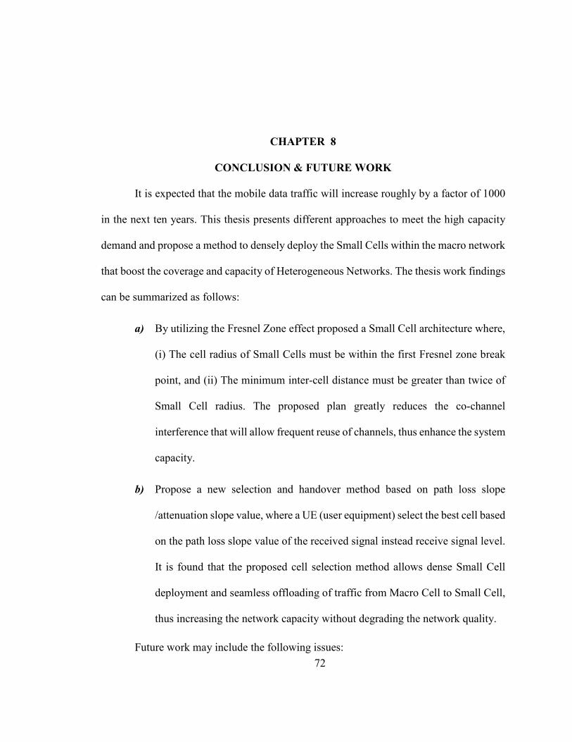
72
CHAPTER 8
CONCLUSION & FUTURE WORK
It is expected that the mobile data traffic will increase roughly by a factor of 1000
in the next ten years. This thesis presents different approaches to meet the high capacity
demand and propose a method to densely deploy the Small Cells within the macro network
that boost the coverage and capacity of Heterogeneous Networks. The thesis work findings
can be summarized as follows:
a) By utilizing the Fresnel Zone effect proposed a Small Cell architecture where,
(i) The cell radius of Small Cells must be within the first Fresnel zone break
point, and (ii) The minimum inter-cell distance must be greater than twice of
Small Cell radius. The proposed plan greatly reduces the co-channel
interference that will allow frequent reuse of channels, thus enhance the system
capacity.
b) Propose a new selection and handover method based on path loss slope
/attenuation slope value, where a UE (user equipment) select the best cell based
on the path loss slope value of the received signal instead receive signal level.
It is found that the proposed cell selection method allows dense Small Cell
deployment and seamless offloading of traffic from Macro Cell to Small Cell,
thus increasing the network capacity without degrading the network quality.
Future work may include the following issues:

73
a) Since Small Cell can be deployed and maintain by the consumer itself, it will
be difficult to maintain the quality of the network in case of dense Small Cell
deployment. So more analysis is needed to explore different deployment
challenges for dense Small Cell networks and find solutions to minimize the
challenges.
b) Analysis the performance of path loss slope based cell selection and handoff
method in terms of call drop probability, probability of handoff failure, and
ping pong rates.
c) Since the radius of small cell is less than a kilometer, the number of handoff
might increase for high speed users. So, more analysis is needed to solve this
mobility problem.

74
APPENDICES

75
Appendix A
Calculating Fresnel Zone Break Point for Different Antenna height MATLAB™ Code %**********************************************************
% Thesis_Code_Final
% Md. Maruf Ahamed
% University of North Dakota
% August 2015
% Finding Freznel Zone Breakpoint for different transmitting antenna height
%**********************************************************
clc;
clear;
close all;
h1=1.5; % receiver antenna height
h2=1:5:30; % transmitter antenna height
f=2100*10^6;
lamda=3*10^8./f;
d=(4*h1*h2)./lamda % fresnel zone break point in meter
plot(h2,d)
grid on
xlabel('Transmitting antenna height h2 in meters', 'FontSize', 11);
ylabel('Cell Radius or fresnel zone break point in meter', 'FontSize', 11);
text(3,126,['\bullet\leftarrow' 'd=50, h2=3m'], 'FontSize', 11)
text(20,840,['\bullet\leftarrow' 'd=294m, h2=20m'],'FontSize', 11)

76
Appendix B
Calculating Fresnel Zone Break Point for Different Operating Frequency MATLAB™
Code %**********************************************************
% Thesis_Code_Final
% Md. Maruf Ahamed
% University of North Dakota
% August 2015
% Finding Fresnel Zone Break Point for Different Operating Frequency
%**********************************************************
clc;
clear;
close all;
h1=1.5; % receiver antenna height
h2=3; % transmitter antenna height for outdoor
f=400*10^6:500*10^6:5900*10^6;
%f=1700*10^6;
lamda=3*10^8./f;
d=(4*h1*h2)./lamda % fresnel zone break point in meter
plot(f,d)
grid on
xlabel('Operating frequency in Hz', 'FontSize', 11);
ylabel('Cell Radius or fresnel zone break point in meter', 'FontSize', 11);

77
text(2100*10^6,126,['\bullet\leftarrow' 'f=2100MHz, d=126'], 'FontSize', 11)
text(3500*10^6,210,['\bullet\leftarrow' 'f=3500MHz, d=210'],'FontSize', 11)
Appendix C
Multipath Effect in Proposed Small Cell Planning MATLAB™ Code
%**********************************************************
% Thesis_Code_Final
% Md. Maruf Ahamed
% University of North Dakota
% August 2015
% Multipath Effect in Proposed Small Cell Planning
%**********************************************************
clc;
clear;
close all;
h1=3; %transmitting antenna height in meter
h2=1.5; % receiving antenna height in meter
f=2100; % operating frequency in MHz
d=(4*h1*h2*f*10^6)/(3*10^8) % fresnel zone break point
RSL=-100;% -70dBm=-70-30=-100dB , Desired Received signal level in dB
ERP=10*log10(10.89/1000); % ERP in dBW
Lp=32.44+20*log10(f)+20*log10(d/1000)
gama=1.5:.5:5;
exp=(ERP-Lp-RSL)./(10*gama)

78
D=d*10.^(exp)
plot(gama,D)
grid on
hold on
ERP=10*log10(70/1000); % ERP in dBW
Lp=32.44+20*log10(f)+20*log10(d/1000)
gama=1.5:.5:5;
exp=(ERP-Lp-RSL)./(10*gama)
D=d*10.^(exp)
plot(gama,D)
hold on
ERP=10*log10(1/1000); % ERP in dBW
Lp=32.44+20*log10(f)+20*log10(d/1000)
gama=1.5:.5:5;
exp=(ERP-Lp-RSL)./(10*gama)
D=d*10.^(exp)
plot(gama,D)
xlabel('Attenuation Slope', 'FontSize', 11);
ylabel('Small Cell Radius in Meters', 'FontSize', 11);

79
Appendix D
Carrier to Interference Analysis MATLAB™ Code %**********************************************************
% Thesis_Code_Final
% Md. Maruf Ahamed
% University of North Dakota
% August 2015
% Carrier to Interference Analysis for different deployment areas
%**********************************************************
clc;
clear;
close all;
%gama=1:.5:4.5; % 2=free space, 2.5=rural, 3=suburban, 3.5=typical urban,4=Dense
Urban
gama=2;
gama2=4; % for dense urban
j=6;
R=420; %for 700MHz LTE, h1=30m, h2=1.5m radius of smll cell
D=500:100:2500 ;%for directional reuse, interferer is 2
CtoI=10.*log10((1./j).*((D./R).^gama))
CtoI2=10.*log10((1./j).*((D./R).^gama2))
plot(D, CtoI)
grid on
xlabel('Inter-cell distance ', 'FontSize', 11);

80
ylabel('Carrier to interference ratio C/I', 'FontSize', 11);
hold on
plot(D, CtoI2)
xlabel('Inter-cell distance in meters', 'FontSize', 11);
ylabel('Carrier to interference ratio C/I in dB', 'FontSize', 11);
text(900,-1.162,['\bullet\leftarrow' 'Path loss slope=2'],'FontSize', 11 )
text(900,5.458,['\bullet\leftarrow' 'Path loss slope=4'], 'FontSize', 11)

81
REFERENCES
[1] "Cisco Visual Networking Index: Global Mobile Data Traffic Forecast Update 2014–2019 White Paper," Cisco, 2015.
[2] "White paper - Enhance Mobile Networks to Deliver 1000 Times More Capacity by 2020," Nokia Solutions and Networks, 2014.
[3] Y. Shu-ping, S. Talwar, W. Geng, N. Himayat, and K. Johnsson, "Capacity and coverage enhancement in heterogeneous networks," Wireless Communications, IEEE, vol. 18, pp. 32-38, 2011.
[4] H. S. Dhillon, "Small Cells, Big Gains: Increasing Cellular Capacity by 1000x," IEEE ComSoc webinar 03/2015.
[5] "Enabling Hyper-Dense Small Cell Deployments with UltraSON," Qualcomm Technologies, Inc., 2014.
[6] L. G. Joydeep Acharya, Sudhanshu Gaur, Heterogeneous Networks in LTE-Advanced: John Wiley & Sons, Ltd, 2014.
[7] M. Noordman, "The role of smalls cells in Heterogeneous Networks," Ericsson AB July 2012
[8] G. d. l. R. Tony Q. S. Quek, İsmail Güvenç, Marios Kountouris, "Small Cell Networks Deployment, PHY Techniques, and Resource Management," ed: Cambridge University Press.
[9] "Heterogeneous Networks," Ericsson White Paper, September 2014.
[10] L. Lu, G. Y. Li, A. L. Swindlehurst, A. Ashikhmin, and Z. Rui, "An Overview of Massive MIMO: Benefits and Challenges," Selected Topics in Signal Processing, IEEE Journal of, vol. 8, pp. 742-758, 2014.
[11] E. Larsson, O. Edfors, F. Tufvesson, and T. Marzetta, "Massive MIMO for next generation wireless systems," Communications Magazine, IEEE, vol. 52, pp. 186-195, 2014.

82
[12] "How can mobile networks deliver 1000 times more capacity by 2020?," Nokia Solutions and Networks, 2015.
[13] S. Geirhofer and P. Gaal, "Coordinated multi point transmission in 3GPP LTE heterogeneous networks," in Globecom Workshops (GC Wkshps), 2012 IEEE, 2012, pp. 608-612.
[14] M. Sawahashi, Y. Kishiyama, A. Morimoto, D. Nishikawa, and M. Tanno, "Coordinated multipoint transmission/reception techniques for LTE-advanced [Coordinated and Distributed MIMO]," Wireless Communications, IEEE, vol. 17, pp. 26-34, 2010.
[15] R. Ratasuk, D. Tolli, and A. Ghosh, "Carrier Aggregation in LTE-Advanced," in Vehicular Technology Conference (VTC 2010-Spring), 2010 IEEE 71st, 2010, pp. 1-5.
[16] M. Iwamura, K. Etemad, F. Mo-Han, R. Nory, and R. Love, "Carrier aggregation framework in 3GPP LTE-advanced [WiMAX/LTE Update]," Communications Magazine, IEEE, vol. 48, pp. 60-67, 2010.
[17] "High-Capacity Indoor Wireless Solutions: Pico Cell or Femtocell?," Fujitsu Network Communications Inc., 2013.
[18] Mehdi Bennis and W. Saad, "An introduction to Wireless Small Cell Networks," IEEE Global Communications Conference 3-7 December 2012.
[19] Q. Tongwei, X. Dengkun, Y. Dongkai, J. Wei, and H. Yuan, "Cell selection analysis in outdoor heterogeneous networks," in Advanced Computer Theory and Engineering (ICACTE), 2010 3rd International Conference on, 2010, pp. V5-554-V5-557.
[20] "3GPP TR 36.932: "Scenarios and requirements for Small Cell enhancements for E-UTRA and E-UTRAN".
[21] "3GPP TR 36.872: "Small Cell enhancements for E-UTRA and E-UTRAN ".
[22] Y. Q. Rose Qingyang Hu Heterogeneous Cellular Networks, 2013.
[23] G. C. King, "Vibrations and Waves," ed, 2009.
[24] H. Xia, H. L. Bertoni, L. R. Maciel, A. Lindsay-Stewart, and R. Rowe, "Radio propagation characteristics for line-of-sight Micro Cellular and personal communications," Antennas and Propagation, IEEE Transactions on, vol. 41, pp. 1439-1447, 1993.
83
[25] S. Faruque, Cellular Mobile Systems Engineering Artech House Mobile Communications, 1997.
[26] T. 3GPP, "Further advancements for E-UTRA physical layer aspects," Mar. 2010.
[27] S. Landstrom, H. Murai, and A. Simonsson, "Deployment Aspects of LTE Pico Nodes," in Communications Workshops (ICC), 2011 IEEE International Conference on, pp. 1-5,2011.
[28] K. Davaslioglu and E. Ayanoglu, "Interference-based cell selection in heterogenous networks," in Information Theory and Applications Workshop (ITA), pp. 1-6,2013.
[29] D. Lopez-Perez, I. Guvenc, and C. Xiaoli, "Theoretical analysis of handover failure and ping-pong rates for heterogeneous networks," in Communications (ICC), 2012 IEEE International Conference on, pp. 6774-6779, 2012.
[30] A. Jabban, Y. Nasser, and M. Helard, "SINR based network selection strategy in integrated heterogeneous networks," in Telecommunications (ICT), 2012 19th International Conference on, pp. 1-6, 2012.
[31] K. Ayyappan, K. Narasimman, and P. Dananjayan, "SINR Based Vertical Handoff Scheme for QoS in Heterogeneous Wireless Networks," in Future Computer and Communication, 2009. ICFCC 2009. International Conference on, pp. 117-121, 2009.
[32] J. Sangiamwong, Y. Saito, N. Miki, T. Abe, S. Nagata, and Y. Okumura, "Investigation on Cell Selection Methods Associated with Inter-cell Interference Coordination in Heterogeneous Networks for LTE-Advanced Downlink," in Wireless Conference 2011 - Sustainable Wireless Technologies (European Wireless), 11th European, pp. 1-6, 2011.
[33] M. A. S. AboulHassan, Essam A.; Shaaban, Shawki, "NOVEL CELL SELECTION PROCEDURE FOR LTE HETNETS BASED ON MATHEMATICAL MODELLING OF PROPORTIONAL FAIR SCHEDULING," International Journal of Wireless & Mobile Networks, vol. 5, p. 37, December 2013.
[34] M. Khan and K. Han, "An Optimized Network Selection and Handover Triggering Scheme for Heterogeneous Self-Organized Wireless Networks," Mathematical Problems in Engineering, vol. 2014, p. 11, 2014.
[35] 3GPP TS36.214, "E-UTRA – Physical Layer Measurements," 12.1.0 ed, 2015.
[36] “Introduction to Wireless Links for Digital Communications: Radio Link Budget”.Retrieved November 29, 2007, from Enigmatic Consulting.

84
[37] Abdul Basit, Syed-"Dimensioning of LTE Network: Description of Models and Tool, Coverage and Capacity Estimation of 3GPP Long Term Evolution radio interface " Master’s Thesis submitted in Helsinki University of Technology.
[38] JJamalipour, A., Mirchandani, V., Kibria, M.R., “Dimensioning of an enhanced 4G/B3G infrastructure for voice traffic,” IEEE 16th International Symposium on Personal, Indoor and Mobile Radio Communications, 2005. PIMRC September 2005.
[39] K. Allsebrook and J. D. Parsons, “Mobile radio propagation in British cities at frequencies in the VHF and UHF bands”, IEEE Transactions. Vehicular Technology, vol. VT-26, pp. 313-322, 1977.
[40] Md. Masud Hasan, Kishore Bhowmik and Md.Maruf Ahamed “Analysis of Cell Planning and Link Budgeting in WiMAX Communication”, IJCSI International Journal of Computer Science Issues, Vol. 9, Issue 3, No 1, ISSN (Online): 1694-0814, May 2012.
[41] P. Bernardin, M. Yee and T. Ellis, “Estimating the range to cell edge from signal strength measurements”, IEEE Vehicular Technology Conference, VTC-1997.
[42] C. E. Shannon, "Communication in the presence of noise", Proc. Institute of Radio Engineers, vol. 37, no.1, pp. 10-21, Jan. 1949. Reprint as classic paper in: Proc. IEEE, Vol. 86, No. 2, 1998
[43] M. Hata, K. Kinoshita and K. Hirade, “Radio Link Design of Cellular Land Mobile Communication Systems”, IEEE Transactions on Vehicular Technology, vol VT 31 February 1982.
[44] M. Hata, K. Kinoshita and K. Hirade, “Radio Link Design of Cellular Land Mobile Communication Systems”, IEEE Transactions on Vehicular Technology, vol VT 31 February 1982.
[45] K. Manoj, P. Bernardin and L. Tamil, “Coverage prediction for cellular networks from limited signal strength measurements, “Ninth IEEE International Symposium on Personal, Indoor and Mobile Radio Communications (PIMRC '98), pp. 1147 – 1151, Sep 1998.
[46] Jun Gu and Ren Sheng, “Research on LTE Network Coverage Planning”, White paper ZTE Communication
[47] RuzIcka, Z. Hanus, S., “Radio Network Dimensioning in UMTS Network Planning Process,” 18th International Conference on AppliedElectromagnetics and Communications, 2005. ICECom October 2005.

85
[48] J.B. Andersen, et al., “Propagation measurements and models for wireless Communications channels, “IEEE Communications Magazine, vol. 33, no.1, pp. 42-49, Jan 1995.
[49] L. C. P. Floriani and G. R. Mateus. Optimization models for effective cell planning design. In Proc. of the 1st Interntaional Workshop on Dis-crete Algorithms and Mehods for Mobile Computing and Communica-tions, 1997.
[50] F. Ikegami, S. Yoshida, T. Takeuchi, and M. Umehira, “Propagation factors controlling mean field strength on urban streets, “ IEEE Transactions on Antennas and Propagation, vol. AP-32, pp. 822-829, 1984
[51] M. L. Rekhi, Sukhvinder Malik, Rahul Atri "Throughput Calculation for LTE TDD and FDD System," White paper, December 2012.
[52] D. T. Ngo, Le-Ngoc, Tho, Architectures of Small-Cell Networks and Interference Management, 2014.
[53] D. X. Tongwei Qu, Dongkia Yang, Wei Jin, Yuan He, "Cell Selection Analysis Outdoor Heterogeneous Networks," 2010 3rd International Conference, Chengdu, vol. 5, pp. 554 – 557, 2010.
[54] E. Seidel, "LTE-A HetNets using Carrier Aggregation," NoMoR Research GmbH, Munich, Germany, June, 2013.
[55] S. Parkvall, A. Furuskar, and E. Dahlman, "Evolution of LTE toward IMT-advanced," Communications Magazine, IEEE, vol. 49, pp. 84-91, 2011.
[56] Qualcomm Inc., "A Comparison of LTE Advanced HetNets and Wi-Fi," 2011.