AALTO UNIVERSITY SCHOOL OF SCIENCE AND TECHNOLOGY Faculty of Electronics, Communications and Automation Networking and Communications Laboratory

Enabling Wireless Sensors Localization in Dynamic Indoor Environments

José Valarezo

Master’s Thesis submitted in partial fulfillment of the requirements for the Degree of Master of Science in Technology

Espoo, April 2010

Supervisor: Professor Riku Jäntti

Instructor: M.Sc. Shekar Nethi

ii

AALTO UNIVERSITY Abstract of the SCHOOL OF SCIENCE AND TECHNOLOGY Master’s Thesis

Author: José Valarezo

Title: Enabling Wireless Sensors Localization in Dynamic Indoor Environments

Date: March 2010 Number of pages: 65 + 33

Department: Department of Electrical and Communications Engineering

Professorship: S-72 Communications Engineering

Supervisor: Professor Riku Jäntti

Instructor: M.Sc. Shekar Nethi

Wireless sensors networks localization is an important area that attracts

significant research interest. Localization is a fundamental problem that must be

solved in order to support location-aware applications. The growing demand of

location-aware applications requires the development of application-oriented

localization solutions with appropriate trade offs between accuracy and costs. The

present thesis seeks to enhance the performance of simple and low-cost

propagation-based localization solutions in dynamic indoor environments.

First, an overview of the different approaches in wireless sensors networks

localization is provided. Next, sources of received signal strength variability are

investigated. Then, the problems of the distance-dependant path loss estimation

caused by the radio channel of dynamic indoor situations are empirically analyzed.

Based on these previous theoretical and empirical analysis, the solution uses spatial

and frequency diversity techniques, in addition to time diversity, in order to create a

better estimator of the distance-dependent path loss by counteracting the random

multipath effect. Furthermore, the solution attempts to account for the random

shadow fading by using “shadowing-independent” path loss estimations in order to

deduce distances. In order to find the unknown sensor’s positions based on the

distance estimates, the solution implements a weighted least-squares algorithm that

reduces the impact of the distance estimates errors on the location estimate.

Keywords: Localization, path loss, received signal strength, wireless sensors networks,

multipath effect, shadow fading, optimization, range

iii

Preface This work has been performed as part of the Wireless sensor systems in indoor

situation modeling (WISM) project and of the Generic sensor network architecture

for wireless automation (GENSEN) project.

I wish to express my sincere thanks and appreciation to my supervisor Riku Jäntti

and my instructor Shekar Nethi for their attention, guidance, insight and support

during this work and preparation of the Thesis. In addition, special thanks to Joni

Silvo for his technical support as well as to Lasse Eriksson and Justus Dahlen for

being part of the process.

I really enjoyed the experience of working in a cooperative and friendly

environment as a member of the Wireless Sensors Networks group at Aalto

University.

I would like to express my gratitude to my family for their unconditional love and

support since my childhood to this level of my career.

José Valarezo

March 2010, Espoo, Finland

iv

Table of Contents ABSTRACT .........................................................................................................................................ii

PREFACE...........................................................................................................................................iii

TABLE OF CONTENTS...................................................................................................................iv

LIST OF ABBREVIATIONS............................................................................................................vi

1 Background on Wireless Sensors Networks Localization 1

1.1 Our field of interest …………………………………………………………2 1.2 Problem definition …………………………………………………………..2 1.3 Methodology ………………………………………………………………..4 1.4 Thesis outline………………………………………………………………..4

2 Localization Approaches in WSN 6

2.1 Range methods ……………………………………………………………...6 2.1.1 Received signal strength …………………………………………….8 2.1.2 Time of flight ………………………………………………………..9 2.1.3 Beamforming ………………………………………………………10 2.1.4 Radio interferometry ………………………………………………11

2.2 Range-free methods ……………………………………………………….12 2.2.1 Connectivity-based ………………………………………………...13 2.2.2 Proximity-based ……………………………………………………14 2.2.3 Fingerprint-based …………………………………………………..15

2.3 Hybrid measurements and solutions ………………………………………15 2.4 Solution approach …………………………………………………………16

3 Development of a Novel Propagation-Based Ranging System 18

3.1 Sources of RSS variability ………………………………………………...18 3.1.1 Extrinsic sources of RSS variability ……………………………….18 3.1.2 Intrinsic sources of RSS variability ………………………………..21

3.2 Path loss modelling ………………………………………………………..22 3.2.1 Distance-dependant signal loss ……………………………………22 3.2.2 Multipath effect ……………………………………………………24 3.2.3 Shadow fading …………………………………………………….29

4 Localization Algorithms 33

4.1 Optimization ……………………………………………………………….34 4.2 Localization algorithm approach ………………………………………….36 4.3 Problem statement …………………………………………………………37 4.4 Least-squares optimization ………………………………………………..37 4.5 Weights function …………………………………………………………..39 4.6 Simulative performance analysis ………………………………………….42 4.6.1 Simulations results ………………………………………………...43

v

5 Empirical Platform 47

5.1 The IEEE 802.15.4 Standard ………………………………………………47 5.1.1 Network topology ………………………………………………….48 5.1.2 Layers ……………………………………………………………...49 5.1.3 Application side ……………………………………………………49

5.2 Sensinodes …………………………………………………………………50 5.2.1 Output power ………………………………………………………51 5.2.2 RSSI / Energy detection …………………………………………...52

6 Solution Demonstration 55

6.1 Creating the application ……………………………………………...……55 6.2 Empirical set-up …………………………………………………………...57 6.3 Results analysis …………………………………………………………....59

6.3.1 Counteracting multipath effect …………………………………….59 6.3.2 Counteracting shadow fading ……………………………………...61 6.3.3 Location estimate ………………………………………………….62

7 Conclusions and Future Work 63

7.1 Conclusions ………………………………………………………………..63 7.2 Future work ….…………………………………………………………….64

References 66

A. Matlab™ source code on the workstation 71

B. C-source code on the measuring nodes 83

C. C-source code on the sink node 91

vi

List of Abbreviations

CDF Cummulative Distribution Function

CSMA-CA Carrier Sense Multiple Access – Collision Avoidance

FFD Full Function Device

GPS Global Positioning System

IEEE Institute of Electrical and Electronics Engineers

LOS Line-of-Sight

LR-WPAN Low-Rate Wireless Personal Area Network

MAC Medium Access Control

MDS Multidimensional Scaling

NLOS Non-Line-of-Sight

PCB Printed Circuit Board

PHY Physical Layer

RSS Received Signal Strength

RSSI Received Signal Strength Indicator

RIPS Radio Interferometric Positioning System

RFD Reduced Function Device

RTS Request-to-Send

RTT Round Trip Time

SS Spread Spectrum

TDOA Time Difference of Arrival

TOF Time-of-Flight

UWB Ultra Wide Band

WLS Weighted Least-Squares

WPAN Wireless Personal Area Network

WSN Wireless Sensors Network

1

CHAPTER 1

Background on Wireless Sensors Networks Localization

The application of wireless networked sensors started in the defense area, providing

capabilities for reconnaissance and surveillance as well as other tactical

applications. Currently, wireless sensor network (WSN) is a relevant technology

that provides solutions for multiple “smart environments”, including industrial

automation, environment and habitat monitoring, healthcare applications, home

automation and traffic control. Low-cost, low-power and multi-functional sensors

that are small in size and communicate in short distances make wireless sensors

networks a suitable technology for large-scale solutions [51].

Localization, also known as location discovery or self-localization, refers to

the ability of a system to deduce the geographical location of a node, which is a

fundamental problem that must be solved in a sensors network. Knowing the

locations of the network nodes is crucial in order to support many applications and

protocols. For instance, ambient monitoring applications require the sensed data to

be stamped with the absolute location. Similarly, actuator networks perform specific

2

functions according to the location information, like for instance the operation of a

crane. Also, traffic-based applications may generate routes based on the location

information.

At the current state, reliable outdoors localization systems based on the

Global Positioning System (GPS) have been successfully deployed during the last

decade for those systems where the form and cost are not major concerns. But,

solving the localization problem in GPS-less indoor environments continue to be

challenging due to major constraints such as non-line-of-sight (NLOS), short-range

measurements and hostile radio propagation properties.

1.1 Our field of interest

Localization is a fundamental problem that must be solved in a wireless sensors

network, which is the field of research of the present Master’s Thesis. The research

seeks to enhance simple and low-cost propagation-based localization solutions for

wireless sensor networks in order to achieve good trade offs between accuracy and

costs.

1.2 Problem definition

Localization algorithms estimate the locations of nodes unaware of their locations

by using previous knowledge of the absolute locations of few nodes and either

range measurements such as distance and bearing measurements, or other network

information such as connectivity maps, proximity information, and signal strength

fingerprints. Nodes with known location information are called anchors, whose

locations can be obtained by using a GPS or by installing them at points with

known coordinates. Nodes that should be localized are called blinds.

There are certainly many issues that make WSN localization a nontrivial

problem. Some of these issues are the costs related to extra localization circuitry

and energy consumption for performing distance and/or bearing measurements,

need of anchors, short-range measurements, inaccurate measurements, non-line-of-

sight, anisotropic networks, and security attacks. Depending on the system

3

requirements and especially on the required localization accuracy of the application,

the aforementioned issues may not enable the realization of a cost-effective

solution.

Acknowledging the increasing demand of many error-tolerant location-aware

applications, a simple and low-cost solution based on the received signal strength

(RSS) is to be designed. Clearly, enabling localization of resource-constrained

sensors in dynamic indoor environments becomes a real challenge due to the special

properties of the radio channel.

The ranging system of the solution uses spatial and frequency diversity

techniques, in addition to time diversity, in order to create a better estimator of the

distance-dependant path loss by counteracting the random multipath effect.

Furthermore, the solution attempts to counteract the random shadow fading by

using “shadowing-independent” path loss estimations for distance prediction1. As it

will be notice later on, path loss estimations are performed online, sidestepping

unpractical offline path loss estimations requiring pre-planning effort and errors of

distance estimates caused by such outdated path loss estimations, as shown in [25].

Ultimately, the solution implements a weighted least-squares localization algorithm

that reduces the impact of distance estimates errors on the location estimate.

The application has been implemented so that it pulls all data from the

network and performs a centralized computation using MATLAB™ since this is

enough to validate the designed solution. Here, the current application supports

single-hop peer-to-peer networks; however, it can be upgraded to support large-

scale multi-hop networks as long as a higher data rate backbone is provided, e.g.,

IEEE 802.11 backbone. Implementing the solution in a decentralized fashion may

be then subject of a future research.

1 Shadow fading and shadow fading are used interchangeably.

4

1.3 Methodology

The work of the present thesis is carried out in four phases. The first phase consists

of an overall study of WSN localization approaches existing in the literature. Thus,

the first phase identifies the different approaches in WSN localization and justifies

the direction of the developed range-based solution.

The second phase consists of an empirical analysis of the problems caused by

the radio channel in dynamic indoor environments. In this phase, a preliminary

measurement campaign in an indoor scenario is required. This empirical analysis

provides the basis for the proposed counteracting approaches in order to reduce the

distance estimates errors.

Before going further to demonstrate the performance of the proposed ranging

system, the third phase provides a simulative performance analysis of distance-

based localization algorithms, i.e., algorithms using distance information in order to

find the blinds’ locations. Simulations are run using MATLAB™ and assume a

certain distribution of the distance estimates errors, i.e., distance between estimated

distance and true distance. Then, the third phase defines a localization algorithm

that reduces the impact of distance estimates errors on the location estimate.

Finally, the fourth phase demonstrates the performance of the designed

propagation-based localization solution. This phase will help us to validate the

proposed counteracting approaches in order to reduce distance estimates errors as

well as to give an insight of the localization accuracy.

1.4 Thesis outline

Localization is a fundamental problem that must be solved in order to support

location-aware applications in wireless sensor and actuator networks. As stated in

[3], no localization approach provides universal positioning services to all

applications. Instead, localization solutions should be application-oriented with

appropriate trade offs between accuracy and costs.

Acknowledging the increasing demand of many error-tolerant location-aware

5

applications, the present research tries to enhance the performance of simple and

low-cost propagation-based localization solutions for IEEE 802.15.4 sensors in

dynamic indoor environments, where the cost and form are major concerns.

Major problems for propagation-based ranging systems2 in indoor situations

are caused by the hostile propagation properties of the radio channel such as

multipath propagation and shadow fading. Acknowledging this, the present solution

seeks to mitigate such problems of path loss estimations without incurring in

unpractical offline calibrations/estimations.

Once the sources of range errors have been addressed, another important

aspect is the localization algorithm itself. There are many algorithms that can be

used for calculating unknown sensors’ locations based on distance information.

Different localization algorithms behave differently, especially in the presence of

range errors. Relevant for the present solution is then to define a robust localization

algorithm in the presence of range errors.

The reminder of the thesis is structured as follows. In Chapter 2, an overview

of the different approaches in WSN localization is provided. In Chapter 3, sources

of RSS variability are first analyzed, and then the path loss estimation of the present

ranging system is discussed. In Chapter 4, the robustness of localization algorithms

in the presence of range errors is analyzed. In Chapter 5, details about the empirical

platform are presented. In Chapter 6, the performances of the proposed ranging

system and of the overall localization solution are analyzed. A brief conclusion and

future work is given in Chapter 7.

2 Systems that estimate distances performing RSS-to-distance mappings based on path loss estimations.

6

CHAPTER 2

Theoretical Study Localization Approaches in WSN

In wireless sensors networks there are several methods intended to solve the

localization problem under different scenarios and for applications with varying

accuracy granularity. The papers [19, 3] present a global overview of the

measurement techniques and approaches in WSN localization. Localization

methods can be broadly categorized into two groups: range methods and range-free

methods.

2.1 Range methods

Range methods localize nodes based on distance and/or bearing measurements.3

These methods use a ranging system to deduce distances and/or angles and then run

a localization algorithm over the range estimates in order to find the blind’s

locations. Distance information is either deduced from amplitude measurements,

time measurements or radio interferometry measurements; whereas, bearing 3 In the literature, the term range is normally used to indicate distance measurements; however, in this context range is also used to refer to bearing measurements since both imply deducing information from measurements.

7

information is either deduced from beamforming measurements or radio

interferometry measurements.

The performance of range methods is mainly determined by the accuracy of

the distance and/or angle estimates. In fact, in [28, 29] the authors have remarked

that the performance of range-based localization systems is limited by the range

errors, and it cannot be significantly improved even using complex localization

algorithms. As a rule of thumb, ranging systems outperforming others require more

complex hardware configurations.

Complex ranging systems are employed for applications requiring fine-

grained localization, i.e., localization accuracy relatively small with respect to the

radio range, where the form and cost are not major concerns. Such systems

commonly use propagation-time measurements of signals with high resolution to

multipath propagation such as acoustic signals [1, 2] or ultra-wideband (UWB)

signals [10, 11]. Lately, radio interferometry techniques are gaining interest since

they can achieve both accuracy and reach for outdoor situations [20], and

apparently for indoor situations as well [21]. However, interferometry-based

ranging systems do not seem to be viable with the current sensors platforms since

they typically require more powerful platforms to make detailed observations of the

signals.

Acknowledging that a wide variety of applications require simple and low-

cost localization systems, propagation-based ranging systems have been widely

investigated. Propagation-based localization solutions are suitable for WSN

localization since they use the built-in Received Signal Strength Indicator (RSSI) of

the sensors radios. However, the accuracy of state-of-the-art propagation-based

localization solutions is questionable, especially for dynamic indoor environments

where the problems of the hostile radio channels, such as multipath propagation and

shadow fading, further increase the localization error, i.e., distance between

estimated location and true location.

On the other hand, localization systems based on bearing measurements lack

8

of popularity due to they require complex antenna configurations and careful

calibration [19], apart that they do not seem to outperform time-based ranging

systems of similar complexity. Next, the main features and problems of the different

range measurements methods are described.

2.1.1 Received signal strength

Signal strength measurements of radio signals are widely used to estimate distances.

In the ideal case, i.e., free space, isotropic radiation, noise-and-interference free, the

received-power change is just determined by the distance between transmitter and

receiver, referred as distance-dependant signal loss hereafter. Unfortunately, real

world scenarios are far away from the ideal case, so that many sources of RSS

variability have to be addressed in order to obtain distance estimates based on the

ideal propagation model. Sources of RSS variability are caused by the radio

channel, the radio platform, and the antenna radiation pattern.4

Major sources of RSS variability are the random both multipath effect and shadow

fading [3]. The multipath effect occurs due to signals are reflected, diffracted, or

scattered, so that the multipath components of a signal add up constructively (signal

is reinforced) and/or destructively (signal is weakened) at the receiver, leading to

dramatic changes in the total received power. On the other hand, shadow fading

occurs when obstructions weaken radio signals. In indoor situations, the problems

caused by the radio channel are exacerbated due to their hostile propagation

properties.

Robust localization systems typically use signals whit high resolution to

multipath components such as acoustic signals and UWB signals. Unfortunately,

acoustic signals have limited reach whereas spread spectrum techniques require

more bandwidth resources, which are limited in practice. Moreover, in the signal

strength approach for sensors localization, the random shadow fading of dynamic

indoor situations is not properly addressed. Therefore, there is certainly room for

improvements of the signal strength approach for localization of IEEE 802.15.4

4 A more detailed description of the sources of RSS variability is provided in Chapter 3.

9

sensors.

2.1.2 Time of flight

Time measurements of acoustic and radio signals are widely used to estimate

distances. In WSN localization, time-of-flight (TOF) measurements of acoustic

signals are commonly the choice to estimate distances accurately. Since the speed of

acoustic signals is relatively slow (approximately 343 m/s, but changes according to

environmental conditions), their transmission delay can be measured by inexpensive

clocks. Moreover, due to their low speed, reflected signals have a significant delay

relative to the line-of-sight (LOS) signal, so that, they can be filtered out. Again,

due to their low speed, the TOF approach of acoustic signals sidesteps the difficult

synchronization problem by using the time-difference-of-arrival (TDOA) technique,

in which the measured time at the receiver is the elapsed time between two signals

transmitted simultaneously by the transmitter: the radio signal, which starts the

counting, and the acoustic signal, which stops the counting. However, as it is

mention in [3], acoustic signals present three main limitations. First, they attenuate

fast with the distance, and thus, they have limited coverage. Second, they require

LOS to obtain the right distance measurement; otherwise, the measured distance

belongs to a reflected path. Third, human hearable acoustic signals are usually not

suitable, and thus, ultrasound signals become the choice. Here, ultrasound signals

are unidirectional, and thus, special radiators need to be arranged in order to achieve

proper coverage, e.g., multiple microphones or a cone reflector [3].

As an alternative to the ultrasound-based TOF approach, UWB radios can be

used to obtain accurate time measurements due to its high resolution to multipath

components [10, 11], but their reach is also limited. Here, UWB-based TOF systems

improve the measurements accuracy at the cost of using specialized hardware to

achieve sampling rates in GHz, sub-nanosecond synchronization and more

bandwidth resources.

On the other hand, distance measurements can also be obtained by measuring

the TOF of radio signals. Since the propagation speed of radio signals is extremely

10

high (approximately 3x108 m/s), precise sub-nanosecond timers are required in

order to measure their TOF. Thus, major sources of measurements errors under this

approach are the clock resolution and precision (drift). In order to avoid the difficult

synchronization problem of one-way time measurements, round-trip-time

measurements can be used; however, the remote processing time has to be filtered

out. In addition, the synchronization problem can also be avoided by measuring

time differences based on time references provided by few highly synchronized

nodes, which are equipped with precise atomic clocks as in the GPS.

In addition to the measurement errors caused by the clock, radio-based TOF

measurements are vulnerable to multipath propagation. Due to their extremely high

speed, the multipath components of a radio signal cannot be resolved in narrow-

band system, thus spread spectrum techniques arise as the choice.

In [3] the authors conclude that distance measurements, i.e., RSS and TOF

measurements, either have low-accuracy or short-range. However, distance

measurements via radio interferometry techniques have been proposed lately; under

which the low-accuracy and short-range measurements problems are partially

solved. Interferometry-based ranging is discussed in Section 2.1.4.

2.1.3 Beamforming

Beamforming refers to the use of the anisotropy reception pattern of an antenna. In

wireless communications, beamforming antennas are used to deduce the direction

of the transmitter. In the common beamforming approach, the decision of the

direction is given by the maximum signal strength when the beam of the receiver,

which has a directive antenna, is rotated electronically or mechanically. A blind’s

location is then approximated based on triangulation principles.

Unfortunately, this method is vulnerable to many sources of signal strength

variability caused by the radio channel and the transceiver. Major sources of error

are the multipath effect and the nonlinearities of the power amplifier at the

transmitter. In theory, narrow beam antennas would diminish problems caused by

multipath effect, whereas, erroneous bearing information caused by the varying

11

transmitted power could be filtered out by normalizing the RSS measurements of

the directional antenna with RSS measurements obtained from an extra

omnidirectional antenna at the receiver [19]. However, complex narrow-beam

antenna configurations are typically challenging and not practical for sensors

networks.

On the other hand, by using a minimum of two (but typically at least four)

stationary antennas with known anisotropic antenna patterns, the direction of the

transmitter can be determined by comparing the signal strength received from each

overlapping antenna. This method eludes the problem of varying signal strength of

absolute measures like in the case of the common directive-antenna method.

However, small measurement errors of signal strength, due to the nonlinearities of

the receiver, typically lead to 10-15° measurement error with four antennas, 5° with

six antennas and 2° with eight antennas [19].

2.1.4 Radio interferometry

Lately, localization systems based on radio interferometry techniques seem to be

promising. Both, distances and bearing information can be deduced via radio

interferometry techniques. Seeking to sidestep the problems of signal strength

measurements, the Radio Interferometric Positioning System (RIPS) [20] estimates

distances by measuring the phase offset between two interfering radio signals which

propagate at slightly different frequencies, so that, the relative phase offset of the

signals received at two different receivers is a function of the distances between the

four transceivers. In theory, the RIPS approach sidesteps two major problems of

signal strength measurements: the antenna orientation problem (RIPS enables three-

dimensional localization) and shadow fading; but, it does not address the multipath

effect problem. In [20], the authors argue that RIPS achieves both accuracy and

range in outdoor environments, solving the low-accuracy and short-range problems

of RSS and TOF distance measurements. The performance of RIPS for the case of

indoor environments is not demonstrated in [20]; however, it is expected to be

highly limited in hostile multipath situations.

12

On the other hand, bearing information can be deduced via radio

interferometry techniques by measuring Doppler shifts with the sensors’ radios [21,

22, 23]. The direction of a moving transmitter can be derived from a Doppler shift.

Hence, the location of the transmitter (blind node) can be approximated when

multiple receivers (anchor nodes) detect the shift. In [22, 23], the authors report that

the frequency change in the Doppler shifts is resistant to multipath interference,

thus, this approach is appropriate even for indoor situations. However, their

experiments were limited to outdoor environments. Notice also that this approach

suits to mobile systems where measurable Doppler shifts can be taken over mobile

nodes. But, in the case of static blinds, the method requires a rotation engine in

order to generate measurable shifts.

Here, even thought radio interferometry techniques seem to be promising,

they require complex ranging systems. Ranging based on radio interferometry

measurements typically requires tight synchronization and scheduling, high clock

stability, multi-frequency transmission calibration and powerful platforms for

making detailed observations on the signals.

2.2 Range-free methods

In light of the costs related to complex ranging systems, researchers have sought

range-free methods to the localization problem in wireless sensor networks [12].

Thus, range-free methods do not perform distance measurements or bearing

measurements; instead, they use other resources such as connectivity maps,

proximity information, or signal strength fingerprints in order to localize blinds.

Thus, any range-free method can be categorized into: connectivity-based,

proximity-based and fingerprint-based.

Generally speaking, range-free methods seem not to solve the fine-grained

localization problem. Range-free methods are meant for applications with relatively

high error-tolerance in the location information. Hence, range-free methods focus

on masking errors through fault tolerance, redundancy, aggregation or other means.

The performance of range-free methods is mainly determined by the amount

13

of resources required in terms of number of anchors and planning effort; similar to

range methods case where the performance of the solution is given by the

complexity of the ranging system.

The simplest range-free methods seek to solve the coarse-grained localization

problem, i.e., localization accuracy in the order of the radio range, for large scale

multi-hop networks based on connectivity maps [16, 17]. Range-free methods based

on connectivity maps perform rather intuitive distance estimations using the

network topology, thus, their accuracy is limited by the large errors of such intuitive

estimations. Seeking to improve the performance of connectivity-based methods,

but without performing the difficult ranging procedure, researchers have sought

localization methods based on proximity information [12, 13, 14, 31]. Proximity

information allows creating location estimators such as centers of gravity [12, 13,

14] as well as distance estimators [31]. In general, proximity-based methods

perform satisfactorily in the presence of relatively high number of anchor nodes

distributed uniformly. Thus, proximity-based methods are suitable for networks

with densely distributed nodes, most of whose locations are unknown. Trying to

eliminate the effects of the radio channel such as multipath effect and shadow

fading, localization systems using signal strength fingerprints have been proposed

[15]. In practice, their suitability to dynamic environments is rather questionable

since they use signal strength maps of outdated channel conditions, apart that they

require considerable preplanning effort. Next, the main features and problems of the

different range-free methods are described.

2.2.1 Connectivity-based

Connectivity-based methods perform distance estimations using the network

topology and then find blinds’ locations using the distance information. Thus,

distances are estimated without using explicit distance measurements such as

amplitude measurements, time measurements or radio interferometry

measurements. Connectivity-based methods are commonly known as shortest-path

or distance-vector methods because they estimate distances based on the number of

hops away over the shortest-path and the average radio range [16, 17]. The average

14

radio range is obtained trough communication between anchors by calculating the

average hop-distance based on the anchor-to-anchor distances (deduced from the

anchors’ locations) and the number of hops away over their corresponding shortest-

paths.

Connectivity-based methods try to alleviate two main problems in large-scale

multi-hop networks, such as short-range measurements and limited number of

anchors, while providing coarse-grained localization. In practice, the suitability of

shortest-path methods is limited by the large errors of the coarse-grained distance

estimates, especially in the case of anisotropic networks, i.e., non-uniform nodes

distribution. Outliers5 can be filtered out by using bound constraints for distance

estimates as in the upper bound approach [44] for locating sensors in concave

areas.

2.2.2 Proximity-based

The main characteristic of range-free methods using proximity information is that

the inferred proximity information relies on the assumption that the signal strength

decays monotonically with the distance. Therefore, these methods are also

vulnerable to random variations of the signal strength that lead to incoherent

proximity information.

Most range-free methods using proximity information localize a blind inside

the intersection area of the polygons formed by the anchor nodes, i.e., center of

gravity [12, 13, 14]. In the literature, such methods are known as area-based

methods [3]. Most area-based methods deduce proximity information by comparing

RSS measurements as in APIT [12] and ROCRSSI [13]. However, a most

sophisticated approach to infer proximity information is used by the kernel-based

learning approach [14]. In the kernel-based learning approach a blind is localized

in two steps. In the first step, called coarse-grained localization, a blind is localized

into some classification areas (regions) by minimizing a kernel function based on

statistical learning theory, which considers some monotonically decay of the signal

5 Values out of an expected range.

15

strength. Then, in the second step, called fine-grained localization, the center of

gravity is calculated, i.e., the intersection of the areas containing the blind node,

which were classified in the first step.

On the other hand, proximity information is also used to deduce distances as

in the proximity-distance map approach [31]. In this approach, blind-to-anchors

distances can be deduced from the known distance between a pair of anchors when

the blind is close enough to one of the anchors. In this way, the approach tries to

avoid outliers as it occurs in with the shortest-path approaches in the case of

anisotropic networks.

Here, proximity-based methods require relatively large number of anchor

nodes fairly deployed either to localize nodes inside areas or to deduce distances.

Thus, these methods are suitable for networks with densely distributed nodes, most

of whose locations are unknown.

2.2.3 Fingerprint-based

Fingerprint-based systems try to eliminate the effects of the radio channel such as

multipath effect and shadow fading. Fingerprint-based systems localize nodes based

on pre-planned site-specific signal strength fingerprints, also called RSS maps.

Apparently, fingerprint-based methods like the RADAR system [15] enable

indoors localization. In practice, the applicability of these methods to dynamic

indoor situations is rather questionable due to the RSS maps obey to different

channel conditions than the actual RSS measurements being used for the mapping.

Moreover, although fingerprint-based methods require significantly fewer anchors

to localize blinds compare to the other range-free methods, they require

considerable preplanning effort indeed.

2.3 Hybrid measurements and solutions

Ranging based on hybrid measurements can improve the accuracy of the range

estimates because measurements errors for different types of measurements come

from different sources. Thus, different types of measurements lead to at least

16

partially independent estimators. Performance improvements can be achieved by

using data fusion techniques to create more accurate and robust estimators out of

independent measurements [19]. Of course, hybrid measurements improve the

range accuracy at the cost of more complex ranging systems that require complex

hardware configurations and implementations [10].

Similarly to hybrid measurements, hybrid range-based and range-free

solutions can improve the overall performance of the solution while coping with

two main problems in multi-hop networks such as short-range measurements and

limited number of anchor nodes. For instance, the two-phase localization algorithm

[30] combines range measurements and a shortest-path method for estimating one-

hop distances and multi-hop distances, respectively. The two-phase localization

algorithm can improve the overall performance of the solution. In a similar way,

combining range measurements and the proximity-distance map approach for

estimating one-hop distances and multi-hop distances, respectively, can also

improve the overall performance of the solution while avoiding outliers in the case

of anisotropic network at the cost of more anchor nodes than in the two-phase

localization algorithm.

2.4 Solution approach

As stated in [3], no localization approach provides universal positioning services to

all applications. Instead, localization solutions should be application-oriented with

appropriate trade offs between accuracy and costs.

Acknowledging the increasing demand of many error-tolerant location-aware

applications, simple and low-cost localization solutions need to be designed. It is

clear that radio-based approaches can potentially provide the best cost-performance

trade off since a radio is available on any wireless node and it is already included in

the power budget. Moreover, among the existing radio-based approaches, the

propagation-based approach remains the simplest in terms of hardware complexity

—sensor radios have an in-built RSSI— and implementation.

Here, the ranging system of the designed solution uses spatial and frequency

17

diversity techniques, in addition to time diversity, in order to create a better

estimator of the path loss by counteracting the multipath effect. Furthermore, the

solution attempts to counteract the shadow fading by using “shadowing-

independent” path loss curves for distance prediction. As it will be notice later on,

the path loss estimations are performed online, sidestepping unpractical offline path

loss estimations requiring pre-planning effort and errors of distance estimates

caused by such outdated path loss estimations. Ultimately, the solution implements

a weighted least-squares localization algorithm that reduces the impact of distance

estimates errors on the location estimate.

18

CHAPTER 3

Development of a novel radio-based ranging system

In the present chapter, sources of received signal strength variability are first

discussed. Then, approaches in order to mitigate major problems of path loss

estimations are proposed.

3.1 Sources of RSS variability

Sources of received signal strength variability can be broadly classified into:

extrinsic and intrinsic. Extrinsic sources are those caused by the properties of the

wireless channel and the antenna radiation pattern, whereas intrinsic sources are

those caused by the radio platform.

3.1.1 Extrinsic sources of RSS variability

This category includes sources of variability caused by the radio channel —fading,

interference and noise— and by the antenna radiation pattern.

19

a) Fading

Major sources of received signal strength variability are caused by the random

fading of the radio channel such as multipath effect and shadow fading. The

multipath effect accounts for the different propagation styles of a signal in a

wireless communication system such as reflection, diffraction, and dispersion.

Multiple components of a signal are then received when multiple communication

paths between transceivers exist. At the receiver, the multipath components of the

signal that arrive in phase add up constructively while the ones that arrive out of

phase add up unconstructively. The total received power is determined by the vector

summation of all multipath components of the signal, leading to random dramatic

changes of the total received power. Unfortunately, in IEEE 802.15.4

communications the multipath components are not resolvable since all received

multipath components of a symbol arrive within the symbol time duration, known

as flat fading.

On the other hand, shadow fading occurs when the propagation path between

transmitter and receiver is obstructed by a dense body with large dimensions

relative to the wave-length, so that secondary waves are formed behind the

obstructing body, reaching the receiver. Here, the random fading of the channel is

the major concern for path loss estimation, which is analyzed in detail in Section

3.2.

b) Interference and additive noise

Interference and additive noise6 can also cause random variations of the received

signal strength. The targeted 2.4 GHz frequency band homes many systems for

unlicensed operations, including hot technologies such as Wi-Fi and ZigBee,

exposing them to interference. Interference is non-stationary and does not affect

equally to all receivers. The level of interference at different receivers varies

according to the corresponding path loss towards the interferer. As it is shown in

[32], interference becomes a significant source of received signal strength

6 Also known as termal noise.

20

variability in the presence of interferers with high activity. Interference cannot be

totally avoided since it is not stationary. However, the carrier sense multiple access

with collision avoidance (CSMA-CA) protocol of the IEEE 802.15.4 sensors tries to

avoid interference by clearing the channel for transmission via its request-to-rend

(RTS) message once it finds the channel idle. The developed ranging system further

avoids interference by using a time-based channel hopping schedule, so that the

channel is changed every new time frame, as well as by discarding measurements

taken over channels that present high activity.7

On the other hand, in indoor environments with the presence of machines and

people the additive noise is not necessarily stationary or same at all receivers. By

using 16 receivers placed at different locations, the overall standard deviation of the

measured additive noise was found to be 1.5 dB. In the developed ranging system,

the additive noise at each receiver is estimated by averaging several energy

measurements when the channel is idle.8 Then, the additive noise affecting the

actual measurements at each receiver is filtered out correspondingly. In practice, the

additive noise is a minor source of RSS variability.

c) Antenna radiation pattern

The radiation pattern of an antenna describes how the antenna radiates energy out

into space or how it receives energy. Each antenna has its own radiation pattern, that

is not uniform, i.e., there are no isotropic radiators. Accordingly, antenna gain is

defined as the ratio of maximum-to-average radiation/reception intensity multiplied

by the efficiency of the antenna.

Propagation-based localization systems typically assume uniform radiation, so

that, the combined gain of the pair wise antennas is a constant in the path loss

model for any relative orientation of the sensors. Unfortunately, there are no

7 The channel activity provides a good measure of the interference level of the channel, and it can be estimated as the average time that the channel is found to be busy, i.e., detected power level is higher than the maximum expected additive noise level. In the present solution, high activity was asummed when the channel is busy more than 30% of the time. 8 The channel is considered to be busy when the detected power level is higher than the maximum expected additive noise level, which in turn depends on the receiver’s sensitivity.

21

isotropic radiators. Hence, a propagation- based localization system is constrained

to the region where the radiation is uniform. In theory, this can only be achieved for

two-dimensional networks, using omnidirectional antennas where all of them

present vertical polarization, provided that the omnidirectional radiation pattern is

uniform within the azimuth. Thus, the present solution targets two-dimensional

networks, but it could also be applied to networks where the difference of antenna

heights is small (no more than a meter), provided that half wave-length dipoles (or

quarter wave-length monopoles) radiate almost uniformly within that region [4].

On the other hand, omnidirectional antennas have to be carefully installed on

the motes platforms, given that the radiation pattern is affected by the electrical

ground of the PCB and its electrical circuits. In [33], the authors show that external

monopoles, mounted a wave-length apart from the PCB, radiate uniformly within

the azimuth, which has been considered in the present solution.

3.1.2 Intrinsic sources of RSS variability

This category includes sources of RSS variability caused by the underlying radio

platform such as the nonlinearities of the power amplifier in the transmitter and

sensitivity in the receiver.

Transmitter variability

As it has been demonstrated in [4], different transmitters behave differently even

when they are equally configured. For a certain transmitter, the actual transmitted

power is close to the configured power level, but not necessarily exactly equal. In

addition, this inaccuracy in the transmitted power varies for different transmitters.9

One approach to mitigate this problem would be to normalize the RSS

measurements with respect to a single transmitter. But, this would require

estimating the inaccuracy in the transmitted power for each transmitter using a

single receiver under invariant conditions, which in turn implies pre-planning effort.

Thus, the present ranging system does not address the RSS variability caused by the

9 Facts of the transmitter’s output power of empirical radio platform are provided in Section 5.2.1.

22

transmitter.

Receiver variability

Similar to the transmitter case, different receivers behave differently even when

they are equally configured, as shown in [4]. This means that the RSS value

recorded is not necessarily the same for different receivers, even when all

parameters affecting RSS variability are kept the same, which obeys to the varying

receivers’ sensitivity.10 The variability of the receivers’ sensitivity can be attributed

to shot noise. Here, the shot noise cannot be estimated as in the case of the additive

noise of the channel since it first depends on the current flow when a packet is

received.

Similar to the transmitter case, one solution to mitigate this problem would be

performing an offline estimation of the shot noise at each receiver by using a single

transmitter under invariant conditions in order to normalize the RSS measurements

with respect to a single receiver. Because offline estimations/calibrations are not

considered in the present solution, the present ranging system does not address the

RSS variability caused by the receiver.

3.2 Path loss modeling

Path loss modeling in wireless networks localization seeks to predict the RSS-to-

distance relation determined by the signal fading and the antenna radiation pattern.

In this section, we first study the physical laws governing the line-of-sight signal

propagation. Then, we analyze the problems of path loss estimations in indoor

situation and introduce novel approaches in order to counteract major sources of

RSS variability such as multipath effect and shadow fading.

3.2.1 Distance-dependant signal loss

The distance-dependant signal loss merely obeys to the case of line-of-sight signal

propagation. Strictly speaking, line-of-sight signal propagation is governed by two

10 Facts of the receiver’s sensitivity of the empirical radio platform are provided in Section 5.2.2.

23

physical phenomenons such as the inverse-square law and the atmospheric

attenuation. From electromagnetism theory, we know that the strength of an

electromagnetic signal, spreading outwards of an ideal isotropic radiator, is

inversely proportional to the square of the distance from it, known as the inverse-

square law. On the other hand, the atmospheric attenuation reduces the intensity of

electromagnetic signals due to absorption or scattering of photons in the

atmosphere. Therefore, prediction of the total change in signal intensity involves

both the inverse-square law and estimation of the atmospheric attenuation over the

path.

The effect of the atmospheric attenuation in relatively small spaces such as

indoor environments can be neglected since its impact on the path loss estimation is

minimal, e.g., attenuation is less than 10dB/km. Then, with basis in the inverse-

square law, which predicts the signal strength some distance apart from the ideal

isotropic source, the amount of detected energy by a receiver standing some

distance apart from the transmitter is calculated by the Friis’ transmission equation,

defined as,

( ) 22

2

4 d

GGPP RT

TR πλ= , (3.1)

where d is the distance between the transmitter and the receiver, PR is the available

power at the antenna’s pins (in Watts), PT is the nominal transmission power, and GT

and GR are the antenna gains of the transmitter and receiver, respectively.

The Friis’ equation puts together the distance-dependant signal loss with the

ability of the receiver’s antenna to capture the electromagnetic radiation (antenna

aperture) and the directivity of the transmitter’s antenna to radiate energy into the

space (antenna gain). Notice that equation (3.1) is the simplified Friis’ transmission

equation that assumes no impedance mismatches and reflections, no atmospheric

attenuation and same antennas' polarization.

In our case, the only necessary requirements for RSS-to-distance prediction

based on the Friis’ transmission equation are: ubiquitous radio platforms, i.e., same

radio module, connectors, feeding cable and antenna in each node, and

24

omnidirectional antennas presenting the same polarizations; provided that the

atmospheric attenuation can be neglected in small spaces and losses due to

impedance mismatches are included in the path loss estimation.

3.2.2 Multipath effect

The Friis’ transmission equation predicts the received power at a receiver located

some distance apart from the transmitter when the line of sight is the unique

propagation path between them. In practice, terrestrial radio communications

normally presents multipath propagation, i.e., multiple propagation paths between

transmitter and receiver, especially in the case of indoor environments where the

surrounding surfaces, furniture and people create multiple propagation paths

between transceivers. Radio propagation models for terrestrial communications

acknowledge the effect of multipath propagation by estimating a path loss exponent

(n) [49, 34] in the standard Friss’ transmission equation as follows,

( ) ⋅=n

RTTR

d

GGPP 2

2

4πλ

(3.2)

For instance, the path loss exponent is typically set to 4 in the two-ray ground

reflection model, which provides accurate signal strength prediction when the

distance apart is much larger than the antenna heights. For convenience, Equation

(3.2) is typically converted to the log-scale, as follows,

][log10][ 100 dPPdRSS T η−+= , (3.3)

where (PT + P0) is the received power at a reference distance of 1 m and η is the

path loss exponent.11 In a typical path loss estimation, where a set of pair-wise RSS

measurements and distances are gathered, (PT + P0) and 10η are respectively

determined by the y-intersection and the absolute value of the slope of the fitted

curve resulting from such set of points, with distances expressed in meters and

converted to the log-scale (x-axis) and received signal strengths expressed in dBm

(y-axis), as shown in Figure 3.2.

Unfortunately, in hostile multipath environments the path loss estimation

11 Recall that the power unit of Equation (3.3) is dBm.

25

above represents the expected received signal strength, but a given measurement

would actually present a random multipath bias (α), also called multipath term, as

follows,

αη +−+= ][log10][ 100 dPPdRSS T . (3.4)

In a preliminary measurement campaign, the fluctuations of the multipath term were

analyzed.12 Figure 3.1 shows the scenario of the preliminary measurements

campaign. Figure 3.2 shows a typical RSS-to-distance curve fitting of data collected

in a static indoor situation. In this figure, a difference of around 20 dB between

measured RSS values corresponding to nearly same distance values can be

observed. This occurs due to one received signal is reinforced by the channel and

the other is weakened.

Figure 3.1: Scenario of the preliminary measurements campaign

12 Worth to recall that, this preliminary measurement campaign was carried out in order to identify the problems of the path loss estimations in indoor situations.

26

Figure 3.2: RSS-to-distance curve fitting (static indoor environment)

Counteracting multipath effect

In IEEE 802.15.4 communications where the multipath components of a signal are

not resolvable, canceling out the multipath effect (or at least averaging it out) is not

as straight forward as averaging some time-independent measurements, especially

in static environments where measurements taken at different time epochs are

highly correlated. In other words, measurements taken at different time epochs are

affected by the same multipath effects in static situations, as it can be observed in

Figure 3.2.13 Therefore, despite time diversity is important in dynamic situations, it

is certainly not enough to mitigate the multipath effect.

Here, considering the random nature of the multipath effect as it is discussed

later on, the following can be stated based on statistical theory:

Statement 3.1: For a pair of transceivers separated a certain distance, if several

RSS measurements over channels presenting independent multipath effects could be

taken, a good estimator of the expected received signal strength can be obtained by

finding the center of the samples distribution.

13 In this figure, measurements belonging to a given link (the ones in circles for instance) differ by few dB, caused by the nonlinearities of the radio platform. However, such measurements present the same multipath fading, e.g., strong signal or deep fading.

0.4 0.5 0.6 0.7 0.8 0.9 1 1.1 1.2 1.3 -90

-85

-80

-75

-70

-65

-60

-55

distance log-scale [m]

Measured samples Path loss model Median of samples

Rec

eive

d P

ower

[dB

m]

Strong signal

Deep fading

27

Here, the median of a set of uncorrelated RSS measurements taken between

two transceivers constitutes a good metric of center –better than the arithmetic

mean– given that the multipath effect phenomenon is not Gaussian; instead, it

presents Rician distribution when there is dominant propagation along the line of

sight between the transmitter and receiver or Rayleigh distribution otherwise [49].

Therefore, the following is assumed:

Assumption 3.1: The median of the distribution of uncorrelated RSS measurements

taken between two transceivers separated a certain distance is an unbiased

estimator of the expected received signal strength.

According to this, equation (3.4) can be restated in terms of the median RSS

(RSSmedian) as follows,

][log10][ 100 dPPdRSS Tmedian η−+= . (3.5)

Finding uncorrelated channels

The present ranging system attempts to find uncorrelated channel in order to obtain

independent (or at least partially independent) RSS measurements, i.e.,

measurements experiencing different multipath effects, for each one-way link via

diversity techniques. In wireless communications, diversity techniques have been

typically used to exploit the random nature of radio propagation by finding

independent channels for communication. On the localization problem side,

diversity techniques allow to create good estimators of the distance-dependant

signal loss out of RSS measurements taken over uncorrelated channels.

The multipath components of a received signal can change with space,

frequency and time. Here, it is known that the total received power is the vector

summation of the multipath components of a signal. In wireless communications,

the differences of the travelled distances of the multipath components of a signal

determine the relative phase offset of these components, which in turn leads to

dramatic changes in the total received power. It can be shown that differences in the

travelled distance of (2n+1)λc among the multipath components of a signal cause

28

them to be flipped in phase.14 For an IEEE 802.15.4 radio operating in the 2.4 GHz

band, a difference of around 12.5 cm between the travelled distances of two

multipath components of a signal causes them to be flipped in phase at the receiver.

The total received power will ultimately depend on the relative phase offsets

of the multipath components of the signal and their strengths at the receiver. Here,

the strengths of the multipath components of a signal and their relative phase offsets

are not only determined by the travelled distances. Whenever an incident radio

signal hits a junction between different dielectric media only a portion of the energy

is reflected and the phase of the signal may be flipped. The amount of reflected

energy and whether the signal is flipped or not depends upon signal polarization,

incident angle, dielectrics, and frequency.

Spatial diversity can be used in order to find channels presenting statistically

uncorrelated multipath effects. The differences of the travelled distances among the

multipath components of a signal at two receivers, whose antennas are slightly apart

of each other,15 are uncorrelated so that the channels among a given transmitter and

these two receivers are also uncorrelated. The channel response at these two

receivers will further differ given that the incident angles of reflected paths among a

given transmitter and these two receivers change, which in turn affects the losses of

reflected components of the signal and possibly their phases. Thus, spatial diversity

effectively allows finding uncorrelated channels in order to perform RSS

measurements.

Similar as above, frequency diversity can be used in order to find channels

presenting statistically uncorrelated multipath effects. Here, the relative phase

offsets of the multipath components of a signal can change with the frequency given

that the differences of the travelled distances of the multipath components of the

signal vary when expressed in terms of different λc.16 In other words, it can be that

the phase offset between two multipath components of a signal is zero at a given

14 λc stands for the wave length of the carrier and (2n+1) stands for all positive odd numbers. 15 It has been empirically shown that the received signals are statistically uncorrelated if the separation between the receiving antennas is just 0.4 wave lengths. 16 The travelled distance is the same but the relation in terms of different λc changes.

29

frequency band, but it is not zero at a different frequency band. Moreover, the losses

of reflected components of a signal and possibly their phases change at different

bands. Thus, frequency diversity allows finding uncorrelated channels in order to

perform RSS measurements.

On the other hand, the time-varying characteristics of the wireless channel can

also be exploited in order to find statistically uncorrelated channels to perform RSS

measurements. In dynamic situations, the multipath components of a signal change

at different time epochs due to the free motion of people or the movement of objects

like mobile cranes. In our case, the coherence time of the channel, a measure of the

expected time duration over which the channel’s response is essentially invariant,

determines the necessary time interval between two consecutive RSS measurements

in order to be taken over uncorrelated channels. For instance, it can be shown that in

a typical office environment the multipath components of a signal at a given

receiver, standing in front of an object or person moving at 1 m/s, change after

around every 100 m/s. Thus, time diversity allows finding uncorrelated channels in

order to perform RSS measurements under dynamic situations. Therefore, spatial,

frequency, and time diversity are used in the present solution in order to perform

RSS measurements over uncorrelated channels.

3.2.3 Shadow fading

Despite diversity techniques allow to create good estimators of the expected

received signal strength out of RSS measurements taken over uncorrelated

channels, it is strictly necessary to consider the effect caused by shadowed paths on

the received power change. In dynamic indoor situations, shadow fading is caused

by the free motion of people, the movement of objects like mobile cranes, or

obstructions like furniture that attenuate the signal.

Figure 3.3 shows a typical RSS-to-distance curve fitting of data collected in a

dynamic indoor situation. In this figure, the median of data clearly presents a

shadowing bias respect to the median of data in the case of static indoor situation

presented in Figure 3.2. This means that the expected received signal strength

30

(median RSS) between a pair of transceivers presents a shadowing bias (ψ), also

called shadow fading term, when the propagation path(s) between transmitter and

receiver are shadowed, so that equation (3.5) is restated as follows,

ψη +−+= ][log10][ 100 dPPdRSS Tmedian . (3.6)

The shadow fading term is generally Gaussian with zero mean and standard

deviation σψ. Here, the shadow fading is a major source of RSS prediction errors

given that its standard deviation ranges from 4 dB to 12 dB depending on the

characteristics of the environment [34].

0.4 0.5 0.6 0.7 0.8 0.9 1 1.1 1.2 1.3-90

-85

-80

-75

-70

-65

-60

-55

distance log-scale [m]

Rec

eive

d P

ower

[dB

m]

Measured samples (static)

Median of samples(static)Measured samples (dynamic)

Median of samples(dynamic)

Figure 3.3: RSS-to-distance curve fitting (dynamic indoor situation)17

Counteracting shadow fading

The present ranging system implements a novel and practical approach in order to

account for the random shadow fading. The solution attempts to account for the

random shadow fading by using “shadowing-independent” path loss estimations for

RSS prediction. Unlike cumbersome approaches such as offline calibrations of the

attenuation introduced by static obstacles, the present ranging system incorporates

the shadow fading affecting the observations in the path loss estimations, which are

calculated online.

17 Dynamic situation data in mustard color and static situation data in light blue color.

31

The shadow fading affecting the observations change at different locations but

it generally presents spatial correlation. Based on this, the following can be assumed

when the observations are made at receivers fixed at the perimeter of a convex area,

Assumption 3.2: Measurements taken at a given receiver are affected by partially

the same shadow fading during a period of time for any relative orientation of the

transmitter, which is independent to the shadow fading affecting measurements

taken at other receivers placed at different locations.

Considering that RSS measurements taken at anchor nodes placed at different

locations experience independent shadow fading, the present ranging system

performs anchor-specific path loss estimations in order to obtain shadowing-

independent path loss estimations, i.e., measurements taken at different anchors are

modeled separately. This means that for a generic i-th anchor node the RSS

measurements are affected by partially same shadowing bias (ψi) during a period of

time, which in turn means that the expected received signal strength (median RSS)

also presents this shadowing bias, so that equation (3.6) can be restated as follows,

iTimedian dPPdRSS ψη +−+= ][log10][ 100 . (3.7)

Based on this belief above, when the path loss estimation and the expected

received signal strength (median RSS) are both calculated using measurements

taken at a certain anchor node during the same period of time, the distance estimates

deduced from such estimations accounting for the shadow fading affecting the

observations are assumed to be unbiased estimates of the true distances. Therefore,

the present ranging considers several18 anchor nodes to be deployed at the perimeter

of a convex area so that a set of pair-wise RSS measurements and their

corresponding known anchor-to-anchor distances can be obtained in order to

perform anchor-specific path loss estimations, where (PT + P0 + ψi) and 10η are

respectively determined by the y-intersection and the absolute value of the slope of

the fitted curves resulting from such set of points. Then, distances are deduced by

mapping the expected received signal strength (median RSS) between each blind-

18 Seven anchor nodes were used in the demonstration presented in Chapter 6.

32

to-anchor and the corresponding anchor-specific path loss estimation.

33

CHAPTER 4

Distance-based localization algorithms

Once the sources of range errors have been addressed another important aspect is

the localization algorithm itself. There are many algorithms that can be used for

calculating the unknown sensors’ locations based on distance information. Such

algorithms are known as distance-based localization algorithms. Different

localization algorithms behave differently, especially in the presence of range

errors. Relevant for the present solution is then to define a robust localization

algorithm in the presence of range errors.

Distance-based localization algorithms can be broadly categorized into: tri-

lateration and optimization. The tri-lateration method is the most basic and intuitive

method that has its basis in geometry principles. This method finds out a blind

location by calculating the intersection of three anchor-centered circumferences —

recall that the two-dimensional solution is considered. The tri-lateration method

achieves perfect localization in the presence of perfect ranging, but it is the worst

performing in the presence of range errors since circumferences do not intersect on

a common point.

34

4.1 Optimization

Distance-based optimization algorithms approximate a blind's location by

minimizing a cost function associated to the distance information. Optimization

algorithms may demand significant computation resources, which depend on the

numerical method used to solve the optimization problem, e.g., Newton-Raphson

method is the most well-known method for real-valued functions.

Optimization problems can also include constraints. Constraints can improve

the convergence of the algorithm. For instance, in the localization problem case,

geometry-based constraints can reduce the impact of range errors on the location

estimate [26]. Also, bounding the fitted distances within an expected range can also

improve the performance of the algorithm [9]. However, constrained optimization

problems commonly demand high computation resources and may lead to

unacceptable convergence times, as shown in [8]. In the present solution, we focus

in unconstrained optimization problems and leave the constrained optimization

problem for future research. Among the most popular optimization algorithms there

are: multilateration, bounding-box, maximum likelihood and global optimization.

Multilateration

The multilateration approach has its basis in the tri-lateration method, but it first

provides a more flexible framework in the presence of range errors. Unlike the tri-

lateration method, which tries to find a blind’s location whose distances to anchors

are exactly equal to the corresponding estimated distances, i.e., distances obtained

from the ranging system, the multilateration approach aims to find a blind’s location

that minimizes the differences between fitted distances and estimated distances. In

the multilateration approach, all estimated distances are equally fitted based on the

belief that they have the same error distribution. Thus, the multilateration approach

finds out the optimal location that is close to the true location with a high

probability [3].

35

Bounding-box

This method, also known as min-max, is popular due to its implementation

simplicity. In the bounding-box algorithm, a blind draws a pair of horizontal lines

and a pair of vertical lines around each anchor, in such a way that the minimum

distance between each line and the anchor location equals the distance estimate

[24]. This algorithm does not achieve perfect localization even in the presence of

perfect ranging.

Maximum likelihood

The maximum likelihood localization technique is based on classical statistical

inference theory [26]. This algorithm finds out a bind's location in which the

probability of receiving the received power matrix within an expected offset is

maximized. This probability is based on the statistical distribution of the range

errors, thus, the maximum likelihood algorithm minimizes the variance of the

localization error as the number of observations, i.e, anchor-originated beacons,

grows to infinity.

Global optimization

Global optimization algorithms try to solve two main problems in large-scale multi-

hop networks such as incomplete ranging, due to short-range measurements, and

limited number of anchors [7, 8, 9]. In the absence of anchors, global optimization

algorithms compute the relative sensors' locations.

In the global optimization approach, all available distance information is used,

i.e., a distance is estimated and used to localize sensors as long as it can be

measured, due to not all blinds have enough surrounding anchors within their radio

range for localizing themselves. Therefore, these methods also use blind-to-blind

distance information to assist the localization process. Unfortunately, using blind-

to-blind distance information may cause the algorithm to calculate a wrong network

map, since the network graph is not fully anchored, and thus, it can have multiple

realizations [19].

36

As an alternative to the global optimization approach, researchers have sought

recursive methods to overcome both, the incomplete ranging problem and limited

number of anchors problem, in large-scale multi-hop networks. In the recursive

methods, a blind whose location is accurately determined becomes a new converted

anchor. Converted anchors are then used to reference other not yet localized blinds

in the network. Hence, the localization process propagates from the area that is

closer to the start-up anchors to the area that is inaccessible to them. However,

localization errors cumulate towards the last localized blinds under this approach.

4.2 Localization algorithm approach

Relevant for the present solution is to define a localization algorithm that reduces

the impact of distance estimates errors on the location estimate. Additionally, we

also seek for trade offs between performance and complexity.

In [24], the authors found that the bounding-box algorithm provides good

trade off between performance and complexity; however, it certainly does not

counteract the impact of distance estimates errors on the location estimate. On the

other hand, the maximum likelihood algorithm tries to reduce the impact of distance

estimates errors on the location estimate at the cost of high complexity [24].

Acknowledging such trade offs, the present solution implements the Weighted

Least-Squares (WLS) algorithm [8], which provides a simpler framework than the

maximum likelihood algorithm while reducing the impact of distance estimates

errors on the location estimate better than the standard distance fitting approaches as

it is explained in Section 4.4.1.

On the other hand, even thought the present solution does not attempt to solve

the global optimization problem, the WLS algorithm can be used to solve the global

optimization problem in the present centralized implementation in case the solution

needs to be upgraded to support large-scale multi-hop networks.

37

4.3 Problem statement

Before going further to study the least-squares approach, we need to define the

generic localization problem. Let’s consider a network of N nodes embedded in the

m dimensional Euclidean space. In the Euclidean space, the distance between nodes

i and j is given by,

[ ]( ) jijiji xxxxDd −== ,, , (4.1)

where D denotes the Euclidean Distance Matrix (EDM), xi denotes the coordinate

vector of node i, and ||• || denotes the Euclidean norm. The Euclidean norm of a

vector v = {v1, v2, … , vm}, where m denotes the dimension of the Euclidean space,

is defined as follows,

22

2

2

1 mvvvv +⋅⋅⋅++= . (4.2)

The Euclidean distance matrix (D) is then defined as the N-by-N symmetric

nonnegative matrix with zeros in the main diagonal composed by all pair-wise

distances of the network graph. The distance estimate between nodes i and j

obtained from the ranging system is denoted by δi,j.

We also define a connectivity matrix (C), where ci,j is a binary value 1/0 that

represents the existence/non-existence of a link between nodes i and j, i.e.,

existence/non-existence of a distance estimate. Also, connectivity level is defined as

the average number of nodes within a radio range. We later refer to completeness as

the ratio between the number of existing distance estimates and the total number of

edges of the fully connected network graph. The term incompleteness refers to the

complement of such ratio.

4.4 Least-squares optimization

Least-squares optimization is an algorithm which allows fitting data based on a

certain criterion (cost function) by approximating the least value of the summation

of the squares of the cost function. In the present solution, the weighted least-

squares [8] algorithm is implemented. The performance of the algorithm will be

compared with a standard least-squares data fitting approach such as metric

Multidimensional Scaling.

38

Multidimensional Scaling (MDS) [27] is a set of methods used to produce a

representation of dissimilarities in a small number of dimensions. In WSN

localization, MDS allows the mapping of the network from the distance

information. Among the different varieties of MDS, metric-MDS is typically used

to solve the global optimization problem in the presence of incomplete and

inaccurate ranging, as shown in [7]. Metric-MDS will be referred just as MDS

hereafter.

Localization problem formulation

MDS and WLS both belong to the nonlinear least-squares optimization family. The

MDS approach aims to find a blind’s location that minimizes the differences

between fitted distances and estimated distances, as follows,

[ ]( )( ) ,,min2

,∑ <ℜ∈−

ji jijiX

xxDmxN

))) δ (4.3)

where X)

is the m-by-N matrix of vector coordinates of the approximated locations

(referred as locations estimates later on). Similar to the multilateration approach, in

the distance fitting approach above all estimated distances are fitted equally based

on the belief that they have the same errors distribution. In fact, when only anchor-

to-blind distance information is used, the MDS resembles the multilateration

approach. However, distance estimates do not necessarily have the same errors

distribution, not at least in the case of propagation-based ranging where the distance

estimate error is proportional to the estimated distance [36], as shown later on.

Acknowledging this, the WLS approach introduces a weights function that accounts

for varying errors distributions of distance estimates.19 This approach showed to

reduce the impact of distance estimates errors on the location estimate [8].

On the other hand, the WLS algorithm not only introduces the aforementioned

weights function, but it also provides a different fitting criterion respect to the

standard least-squares distance fitting approach such as MDS. Here, the WLS aims

to find a blind’s location that minimizes the differences between fitted distances

squares and estimated distances squares, as shown below,

19 A detailed description of the weights function is provided in the next section.

39

[ ]( )( ) ,,min222

,,∑ <ℜ∈−

ji jijijiX

xxDhmxN

))) δ (4.4)

where hi,j represents the weight of the corresponding δi,j distance estimate. In [47],

the authors argue that this distance fitting approach guarantees that the matrix of

fitted distances is a Euclidean distance matrix indeed. In [8], the authors argue that

this fitting approach is robust to severe incompleteness apart that it does not

demand significant computational resources since it allows using Newtown

methods. However, a performance comparison of the WLS respect to a standard

least-squares fitting approaches, such as the MDS, has not been provided. In

Section 4.6, the performance of the MDS and WLS is then compared via extensive

simulations.

4.5 Weights function

The weights function is intended to weight the contribution of each distance

estimate for minimizing the cost function. In the absence of optimality theory, and

considering other techniques that calculate weights based only on intuition as in

[48], where weights are proportional to the number of hops away in the network

that corresponds to the estimated distance, the weights function proposed in [46] is

used in the present solution. Under this weights function, each entry of the weights

matrix is proportional to the relevance of the corresponding entry of the matrix of

distance estimates. The matrix of weights is mathematized based on two

independent factors: the confidence on the distance estimates (HD), and the impact

that each edge has on the rigidity of the network graph (HC) as follows,

CD HHH •= , (4.5)

where the product above implies element-wise multiplication. Notice that the matrix

of weights is a symmetric nonnegative matrix.

Confidence matrix (HD)

The confidence matrix measures the confidence on the distances estimates δi,j

obtained from the ranging system. Each entry of the confidence matrix is calculated

as follows,

40

( ) ( )

⋅⋅−

−

⋅⋅+

−≈jiji

ji

jijijiji

D

KQ

KQh

,,

, 22,,,,

δδ σρα

σρα

)) , (4.6)

so that jiDh, represents the probability that the distance estimate δi,j, conditioned to

the amount of offset ρi,j, is within a range α close to the true distance di,j; where ji ,δσ)

is the sample standard deviation of δi,j computed from the available Ki,j

measurements samples, and Q(x) is the Gaussian Q-function over a value x defined

as follows,

∫∞

−=

x

duu

xQ .2

exp2

1)(

2

π (4.7)

In [46], the authors do not provide an optimality theory for setting α in equation

(4.6), instead it is only mentioned that better accuracy can be achieved on average

for small values of α at the price of larger variance.20

Notice that the offset ρi,j allows accounting for varying errors distributions of

distance estimates. The errors distributions of the distance estimates depends on the

accuracy of the prediction of the received signal strength expressed in dBm. Even

after any efforts to counteract the sources of received signal strength variability, the

prediction of the received signal strength will ultimately be affected by some

generally Gaussian random error (ε) as follows,

ε+= ][][ dRSSdRSS trueprediction , (4.8)

where RSSprediction represents the RSSmedian in equation (3.7). This error in the

received signal strength prediction will lead to a random distance estimate error

proportional to the estimated distance as follows,

= ηε

δ 1010trued , (4.9) where η denotes the path loss exponent as defined in equation (3.2). The equation

above relates to the proportional distance estimate error of a particular estimated

distance, so that the expected proportional error of the distance estimates is given

by,

20 The authors in [46] use α equal to 0.1 m and 1 m, but in the present solution the value was set to 1 m acknowledging the large errors of propagation-based ranging.

41

[ ]

=

=2

10

10log

2

1exp

10

10logexp

ησ

ηεδ ε

truetrue dEdE , (4.10)

where σε is for the resulting standard error of the curve fitting for the corresponding

path loss estimation. Finally, the offset ρi,j conditioning the accuracy of the

estimated distance δi,j is also proportional to the estimated distance and is defined as

follows,

,10

10log

2

1exp1

2

,,

−−≈η

σδρ εjiji (4.11)

Structural matrix (H C)

The structural matrix relates to the impact that the presence/absence of each edge

has on the overall structure of the network graph, regardless of how good or bad the

distance is estimated. The structural matrix measures then the relevance that each

edge has on the rigidity of the network graph.

In [46], the impact that the presence/absence of an edge has on the overall

structure of the network graph is estimated by calculating the amount of

perturbation that the deletion of the edge (i, j) has on the spectrum of the graph.

This perturbation is calculated as shown below,

,G

GpG

Λ

Λ−Λ≅τ (4.12)

where ||• || denotes the Euclidean norm and ΛG and ΛGp are the vectors of

eigenvalues of the representation matrices of the non-perturbed graph Gp and

perturbed graph G, respectively. The representation matrix considered by the

authors in [2] is the signless Laplacian matrix,

L ≅ Θ + C, (4.13)

where Θ is a diagonal matrix where each entry of the main diagonal is equal to the

number of links that the node corresponding to the underlying entry has with other

nodes in the actual network and C is the connectivity matrix.

From the above, we finally arrive at,

42

,)max(, ∆

≅ rC ji

hτ

(4.14)

where the sub-index r refers to the edge connecting nodes (i, j) and ∆ = {τ1, … , τ|E|}

is the set of calculated perturbations, where |E| represents all existing links in the

network.

4.6 Simulative performance analysis

In the present simulative analysis performed in a Matlab™ environment, we seek to

determine the validity of the WLS distance fitting approach and the weights

function.

In order to realize the following simulations, a certain scenario and the errors

distributions of the distance estimates have to be assumed. Thus, a 10x10 squared-

meter room for a range of 7-35 randomly and identically distributed nodes is

considered. The minimum number of anchor nodes (m+1) is considered, where m is

the dimensions of the solution. The radio range (R) is set to 8.5 m, so that more than

70% of the inter-node distances are always detected, i.e., a partially connected

network is considered. The distance estimates are generated using equation (4.9),

where the standard deviation of the prediction error of the received signal strength

(σε) is set to 6 dB and the path loss exponent (η) to 1.64.21 The mean distance

estimates errors of such model was observed to be 4 m when the maximum error is

bounded to half of the radio range, which is in conciliation with real cases [2, 3].

For convenience, the performance of the algorithms is measured in terms of

the mean relative error of the fitted distances, as shown below,

[ ]( ) [ ]( )RAM

xxDxxDji jiji

)(

,,

−

−=∑ <

))

ς , ∀ i ∨ j ∉q, (4.15)

where q is defined as the set of indexes of location vectors of the anchors, M refers

to the number of combinations (i, j) ∀ i ≠ j (M equals to N(N-1)/2 ), and A refers to

the number edges connecting the anchor nodes (A equals to m(m+1)/2 ).

21 This reference values are based on empirical estimations in [24].

43

4.6.1 Simulations results

As it can be noticed, all figures obtained from the simulations present a remarkable

breakpoint at N equals to 15. This behavior is explained by the fact that a blind node

can be localized more accurately as the number of reference points grows to

infinity. In the simulation scenario, the assumed nodes distribution (independent

normal distributions centered at the origin for each axis) leads to high completeness

ratio in the presence of few nodes, but then this ratio decreases as the number of

nodes increases, until it stabilizes to around 75% completeness for N higher than 15

nodes. Hence, the distance fitting errors grow until N equals to 15 nodes due to the

decreasing completeness ratios, but the distance fitting errors start then to reduce

due to the connectivity level increases gradually.

Least-Squares optimization

In the first set of simulations, corresponding to Figure 4.1, the performance between

WLS and MDS is compared. Here, (hi,j) of the WLS cost function (equation (4.4)) is

given by the (ci,j) entry of the connectivity matrix (C), so that only existing

distances estimates given the network connectivity are actually fitted and the non-

existing distance estimates are shunned down in the minimization of the cost

function. This approach before is also used in the minimization of the MDS cost

function, so that the performance of these two different distance fitting criterions

can be compared under the same conditions.22

It can be noticed that both distance fitting approaches lead to similar

performance on average, where MDS outperforms by around 1% only. Although in

[8] it is argued that WLS is more robust than MDS in the presence of severe

incompleteness, there is nothing said about robustness in the presence of distance

estimates errors. Despite we do not focus on the incompleteness problem, this could

be alleviated by forming local maps with good connectivity model on which the

locations are estimated, so that these local maps are then aligned together based on

their common nodes, as it is done in [10]. More relevant for the present solution 22 Notations like for instance MDS(C) in the figures of the present chapter mean that the MDS algorithm with the matrix of weights C was used and so on.

44

becomes robustness in the presence of distance estimates errors, where the WLS

and MDS fitting approaches perform similarly.

10 15 20 25 30 350.19

0.195

0.2

0.205

0.21

0.215

0.22

0.225

0.23

0.235

number of nodes

Mea

n R

elat

ive

Err

or

WLS(C)

MDS(C)

Figure 4.1: Performance comparison between MDS and WLS

On the other hand, it was observed that the WLS algorithm converges faster

than the MDS algorithm, where the convergence time of this first is less than a

second on average. In the present study, the sensitivity of the algorithms with

respect to the parameters σε and η affecting the errors distribution of the distance

estimates according to equation (4.9) is not analyzed. Nevertheless, as a rule of

thumb, the distance fitting accuracy, and in turn the localization accuracy, increases

as the errors of the distance estimates decreases, and according to the errors

distribution of the distance estimates under the received signal strength approach

(equation (4.9)), the errors of the distance estimates decreases as σε and/or 1/η

decreases and vice versa.

Weights function

In the second set of simulations, corresponding to Figures 4.2 and 4.3, the

connectivity matrix (C), the confidence matrix (HD), and the matrix of weights (H)

are evaluated. Figures 4.2 and 4.3 respectively show the performance of the MDS

and WLS algorithm when different matrices of weights are used. It can be observed

that the matrices HD and H lead to roughly 5% gain on average over the

connectivity matrix C. However, this gain increases as the connectivity level, and in

45

turn the number of reference points, grows to infinity.

In [46], it is shown that this gain is around 25% under different conditions.

Nevertheless, after performing extensive simulations this gain could not be

achieved under the assumed scenario and errors distributions of the distance

estimates. Of course, the achieved gain increases as the number of available

samples for each distance estimate (Ki,j in equation (4.6)) grows to infinity;

however, in the present simulations the number of available samples (Ki,j) was set to

20 as it would most likely be in practice.23

On the other hand, as stated in [46] and as it can also be observed from

Figures 4.2 and 4.3, the structural matrix (HC) is less relevant than the confidence

matrix (HD) since matrices HD and H both achieve almost the same gain over the

connectivity matrix C.

10 15 20 25 30 350.16

0.17

0.18

0.19

0.2

0.21

0.22

number of nodes

Mea

n R

elat

ive

Err

or

MDS(C)

MDS(Hd)

MDS(H)

Figure 4.2: Performance comparison of the matrices of weights C, HD, and H over the

MDS algorithm

23 The sensitivity of the different parameters in the weights function of equation (4.6) is discussed in [46].

46

10 15 20 25 30 350.15

0.16

0.17

0.18

0.19

0.2

0.21

0.22

0.23

0.24

number of nodes

Mea

n R

elat

ive

Err

or

WLS(C)

WLS(Hd)

WLS(H)

Figure 4.3: Performance comparison of the matrices of weights C, HD, and H over the

WLS algorithm

Conclusions

It is clear that the weights function reduces the impact of distance estimates errors

on the location estimate and that the achieved gain increases as the number of

available samples for each distance estimate grows to infinity. On the other hand,

even thought MDS and WLS distance fitting approaches provide similar distance

fitting accuracy, the present solution implements the WLS algorithm since it

converges faster and becomes an asset in the presence of severe incompleteness in

case the solution needs to be upgraded to support large-scale multi-hop networks.

47

CHAPTER 5

Empirical platform

Before going further to the empirical demonstration of the proposed solution in

Chapter 6, it is necessary to revise some relevant details of the targeted IEEE

802.15.4 standard compliant motes. Sensinodes are the motes used by the Wireless

Sensor Group at Aalto University. The present chapter consists on a small

description of the IEEE 802.15.4 Standard [43] and the Sensinodes motes [41].

5.1 The IEEE 802.15.4 Standard

The IEEE 802.15.4 standard provides the specifications of the Physical Layer

(PHY) and Media Access Control (MAC) for Low-Rate Wireless Personal Area

Networks (LR-WPANs). LR-WPAN targets low-rate, low-power and low-cost

applications by providing reliable short-range communications.

In the standard, two types of network node are defined: a full-function device

(FFD) or a reduced-function device (RFD). The FFDs can either act as coordinators

or as normal devices. Every WPAN needs at least an FFD to work as the

coordinator of the network. Whereas, the RFDs cannot act as coordinators and they

can only be connected to one FFD at a time. RFDs are merely used for very simple

48

applications that require minimum capabilities.

5.1.1 Network topology

In IEEE 802.15.4 networks, nodes can be arranged into a star or a peer-to-peer

topology, as shown in Figure 5.1.

Figure 5.1: Network topologies24

In the star topology, one node acts as the network controller, known as the

PAN coordinator. The controller is mainly controlling and routing the

communication between nodes in the network, but it can also have other roles

according to the application strategy. In a star topology, reliability of

communications merely depends on the coordinator.

In the peer-to-peer topology, networks nodes communicate in a mesh-like

fashion as long as connectivity exists, where communication paths could be of

multiple hops, i.e., ad-hoc. Thus, communications require self-organization and

management. Routing a message is then more complex, but more reliable.

A star topology is typically used for applications with defined communication

patterns such as home automation, computer peripherals, healthcare applications,

toys and games; whereas, a peer-to-peer topology is used in applications with

undefined communication patterns such as wireless sensor networks for ambient

and habitat monitoring, traffic control and industrial control and monitoring.

Localization solutions generally assume peer-to-peer communications, so that

24 Figure 5.1 has been taken from the IEEE 802.15.4 Standard specifications [43].

49

any node-to-node information can be obtained as long as connectivity exists.

5.1.2 Layers

The IEEE 802.15.4 standard defines specific attributes of the physical layer (PHY)

and the medium access control (MAC) sublayer [43]. The physical layer is

responsible for managing the physical transceiver, whereas the median access

control sublayer is responsible for handling all access to the physical radio channel.

Relevant for the present solution is the inter-system interference.

Three possible unlicensed frequency bands are defined: 868 MHz band, 915

MHz band and 2.4 GHz band. IEEE 802.15.4 systems are then subjected to inter-

system interference. The first band is used in Europe, allowing one communication

channel (868.0-868.6 MHz). The second band is used in North America, allowing

up to ten channels (902-928 MHz). The targeted 2.4 GHz band is used worldwide,

providing 16 radio channels for unlicensed operations. Adjacent channels are 5

MHz apart, ranging from 2405 MHz up to 2480 MHz.

The 2.4 GHz frequency band homes many systems for unlicensed operations,

including hot technologies such as Wi-Fi and ZigBee, where this last is in

compliance with the IEEE 802.15.4 standard. Here, Wi-Fi channels may overlap

with ZigBee channels even though they do not share same carriers. Therefore, apart

from the CSMA-CA protocol of the IEEE 802.15.4 sensors, which tries to avoid

interference by clearing the channel for transmission via its RTS message once it

finds the channel idle, a time-based channel hopping schedule is used in the solution

to further avoid interference.

5.1.3 Application side

When designing applications for wireless sensor networks major issues are power

consumption and scalability.

Sensor networks are often used for monitoring situations where access is

difficult, hazardous or expensive. Lifetime of the network elements must be then

maximized in order to avoid maintenance operations. Elements lifetime depend

50

mainly on the batteries lifetime as long as the elements are used in the correct

conditions [42]. Therefore, power-aware applications should be developed in order

to maximize the batteries lifetime.

In the IEEE 802.15.4 standard, device power management is addressed via the

sleep mode. Then, the time the application spends in sleep mode should be

maximized. In event-driven applications, the sleep interval would ultimately depend

on the frequency of the events occurrence. Then, the sleep interval of the

localization application will depend on how often targets need to be localized,

which in turn depends on their movement speed.

Another important aspect that affects the power consumption and determines

the scalability of the application indeed is the amount of traffic the application

generates. Here, decentralized approaches generally scale better than centralized

approaches. However, the main goal of the present thesis is to mitigate the problems

of propagation-based localization solutions caused by the radio channel of dynamic

indoor environments; thus, a centralized solution has been implemented to validate

the present design.

Implementing the solution in a distributed fashion may be subject of a future

research. However, the present centralized implementation can be upgraded to

support large-scale networks as long as a higher data rate backbone is provided,

e.g., IEEE 802.11 backbone. Then, the large-scale localization problem would be

reduced either to align local maps together, in the presence of sufficient anchors

surrounding each blind, or to solve a global optimization problem otherwise.

5.2 Sensinodes

Sensinodes provides low-power wireless modules for use in sensor networks.

Sensinodes have the NanoStack™ protocol stack that is embedded networking

software supporting low-power IP-based applications running on top of IEEE

802.15.4 radios and operating at the 2.4 GHz frequency band [41].

In the experiments, the U100 micro.2420 sensinode is used (see figure 5.2),

51

which is a fully operable standalone communication node with accessible

connectors for integration of sensors and elements [37]. It has the MSP430

microcontroller and IEEE 802.15.4 compliant CC2420 radio transceiver [40], both

provided by Chipcon. The radio allows 250 kbps data rate and a transmission range

of 100 m with its on-board antenna.

Figure 5.2: U100 micro.2420 sensinode

The microcontroller and radio can be programmed with both, the FreeRTOS

[38] and TinyOS [39] operating systems, which are portable, open source, real-time

operating systems.

In FreeRTOS applications are written in C programming language, whereas in

TinyOS applications are written in NesC [45], which is a programming language

targeting networked embedded systems that has its basis in C. In addition, task

scheduling in TinyOS does not allow threads, whereas FreeRTOS allows pre-

emptive and multi-threading task scheduling, i.e., tasks are served at real time

according to their priority.

5.2.1 Output power

In the CC2420 radio chip, the output power level of the radio transmitter can be

controlled by configuring the TXCTRL.PA_LEVEL register. Table 5.1 shows the

output power for different TXCTRL.PA_LEVEL values. Notice that the

TXCTRL.PA_LEVEL register consist of 5 bits, thus, 32 configurable output power

levels are possible. However, the output power levels in Table 5.1 are the only ones

52

specified in the CC2420 radio chip specifications [40].

PA_LEVEL Output Power [dBm]

31 0

27 -1

23 -3

19 -5

15 -7

11 -10

7 -15

3 -25

Table 5.1: Output power settings @ 2.45 GHz

Output power variability

As before mentioned in Section 3.1.2, the actual transmitted power is close to the

configured power level but not necessarily exactly equal. Furthermore, different

transmitters behave differently even when they are configured in the same way. In

[4], the overall standard deviation of the transmitted power inaccuracy was found to

be 2.24 dB. The results were obtained using a single receiver and 9 different

transmitters, where the CC2420 radio chip was used.

5.2.2 RSSI / Energy detection

The CC2420 radio chip provides an RSSI (Received Signal Strength Indicator) for

energy detection of the channel, which value can be read from the RSSI.RSSI_VAL

register. In compliant to the IEEE 802.15.4 specifications, the RSSI is always

averaged over 8 symbol periods (128 µs).

Figure 5.3 shows a typical RSSI register value vs. input power curve. In

figure 5.3, one can notice that, in accordance to the CC2420 radio chip

specifications [40], the RSSI register value has an offset of roughly -45 as follows:

RFpower(dBm) = −45 + RSSIregister_value 5.1

53

Figure 5.3: Typical RSSI value vs. input power

Energy detection procedures

There are two types of procedures for energy detection: energy detection at packet

reception and continuous energy detection.

In the first type, the measured RSSI is averaged over the 8 symbol periods

following the SFD (Start of Frame Delimiter) of the received packet. The measured

RSSI value is then appended to the second last byte of the received packet. This

value needs to be handled by the application for making any distance estimations

based on the received signal strength.

In the second type, the RSSI value is continuously calculated and updated

every symbol period while the radio is enabled. This updated RSSI value can be

read from the RSSI.RSSI_VAL register. In fact, the designed application performs

noise sensing by reading the aforementioned register.

Energy detection variability

Energy detection with the CC2420 radio chip is very linear as it can be observed in

figure 5.3, but not accurate with respect to the true power. In fact, the typical energy

detection linearity and accuracy with the CC2420 radio chip are ± 3 dB and ± 6 dB,

respectively [40].

54

Moreover, the nonlinearities in the energy detection vary for different

receivers. In other words, the RSSI value recorded is not necessarily the same for

different receivers even if all other parameters affecting RSS variability are kept the

same. In [4], the overall standard deviation of the energy detection inaccuracy for

packet reception was found to be 1.86 dB. The results were obtained using a single

transmitter and 5 different receivers, where the CC2420 radio chip was used.

55

CHAPTER 6

Solution demonstration

In the present chapter, the performance of the present localization solution is

demonstrated. Here, before going further to analyze the results of the solution

demonstration, we first review how the localization application works and the

empirical set-up considered for the experiment. Then, the empirical set-up and the

results are

6.1 Creating the localization application

The localization application has been implemented so that it first pulls data from the

network and then performs a centralized computation using Matlab™ since this is

enough to validate the designed solution. This means that the actual estimations of

distances and locations are centrally calculated after the necessary energy

measurements (RSSI values) for such estimations are pulled from the network.

The localization application performs a round of energy measurements every

time blinds’ need to be localized, so that the path loss estimations and

corresponding distance estimations are performed online based on energy

measurements taken during the same period of time in order to sidestep unpractical

56

offline path loss estimations requiring pre-planning effort and errors of distance

estimates caused by such outdated path loss estimations. Notice that the path loss

estimations are calculated using the well-know anchor-to-anchor distances and the

corresponding energy measurements, then the anchor-to-blind energy measurements

are mapped to distances using those path loss estimations so that the blinds’

locations can be finally estimated based on this anchor-to-blind distance

information.25

During a round of energy measurements each anchor and blind node

broadcasts beacons based on a time schedule in order to both avoid collisions and

enable time diversity for energy measurements. So, beacons are needed to perform

energy measurements and they contain two fields: source ID and packet number,

which are used for the centralized processing of the data. Each anchor and blind

node broadcasts the same number of beacons, one beacon within a time frame. In

every next time frame the radio channel is changed to the next channel of a fixed

sequence of four channels (given as input to the localization application) in order to

both enable frequency diversity for energy measurements and reduce the impact of

radio interference. Each network node represents a dual-node, i.e., two radio

modules and antennas, where the two antennas are placed a wave length apart (12.5

cm approximately) of each other in order to enable spatial diversity for energy

measurements. Finally, each node measures the energy of the channel after every

packet reception in order to estimate the additive noise at each receiver.

Localization entities

In accordance to this above, localization requires three entities:

• Workstation: A workstation supporting a Matlab™ environment where the

estimations of the distances and locations are performed using the energy

measurements pulled from the network and the well-known locations of the

anchor nodes given as input to the application. The source code is included

25 The ranging system and localization algorithms are explain in detail in Chapter 3 and 4, respectively.

57

in Appendix- A.

• Measuring node: A device that performs energy measurements during a

measurements round. A measuring node can be either an anchor node (a

stationary device with a well-known location) or a blind node (a device

which location needs to be calculated). The measuring node is programmed

in C language and its source code is included in Appendix- B.

• Sink node: A device attached to the workstation that initializes the

measurements round and acts as a gateway for the measuring nodes. After

the measurements round ends the sink node collects and passes on

measurements data from each measuring node to the Matlab™ application

on the workstation via serial communication. The sink node can be used as

an anchor node when its location is well-known since it has been

implemented so that it performs energy measurements during the

measurements round. The sink node is programmed in C language and its

source code is included in Appendix- C.

6.2 Empirical set-up

The present experiment was carried out in a typical dynamic indoor situation with

the presence of furniture and mobile objects. For easier monitoring, the selected

indoor scenario is a 13x9 squared-meters room in the Electrical and

Communications Department of Aalto University, shown in Figure 6.2 (left side).

All nodes were deployed 1.3 m from the floor reference, where the ceiling is at 3 m.

Seven anchor nodes deployed as shown in Figure 6.2 (right side) were used.

As before mentioned, the U100 micro.2420 sensinode is used as the

ubiquitous device for the empirical demonstration of the solution. Each radio

module was equipped with an external monopole antenna mounted a wave length

apart from the PCB, as shown in Figure 6.1, in order to reduce the impact of the

electrical components and ground of the PCB on the antenna radiation pattern.

58

Figure 6.1: Empirical scenario (left side), Anchor nodes deployment (right side)

Figure 6.2: External monopole antenna

Parameters configuration

An important aspect of the experiment becomes the parameters configuration such

as the output power, time interval between consecutive beacons, channel hopping

sequence, and number of beacons that each node broadcasts. The CC2420 radio

module supports a range of discrete power settings from -25 dBm until 0 dBm. In

the present experiment, the output power is set to -7 dBm since measurements are

blurred by the background noise when the output power is too low, e.g., -25 dBm,

or too much reflections are generated when the output power is too high, e.g., 0

dBm. Here, setting up the output power to -7 dBm showed to achieve a radio range

of about 15 m, on average. Notice that, in dynamic indoor environments the radio

range is typically reduced due to multipath effect and shadow fading and it can not

be accurately determined.

When setting the time interval between consecutive beacons, it is important to

59

consider the time coherence of the channel in order to enable time diversity for RSS

measurements. Each beacon is then transmitted every next time coherence of the

channel. In a typical office room, where the maximum motion speed a person is

around 1 m/s, the time coherence of the channel is below 100 ms. Thus, the

following experiment uses 100 ms as the time interval between consecutive

beacons. On the other hand, seeking to enable frequency diversity for RSS

measurements while avoiding interference, the channel hopping sequence was

chosen so that any two consecutive channels in the four-channel sequence are at

least four carriers apart of each other, as follows: (2410, 2435, 2455, 2480) MHz.

Finally, in the present experiment, each node broadcasts 20 beacons every time

blinds need to be localized, which provides a meaningful number of samples for

distance estimations.

Parameters Value Output power -7 dBm

Time interval between consecutive beacons 100 ms

Channel hopping sequence (2410, 2435, 2455, 2480) MHz

Number of beacons per node 20

Table 6.1: Parameters values used in the experiment

6.3 Results analysis

Once the implemented localization algorithm showed to reduce the impact of

distance estimates errors on the location estimate in Chapter 4, our aim in this

section is to validate the use of diversity techniques in order to obtain good

estimators of the path loss and the use of anchor-specific path loss estimations in

order to account for the independent shadow fading affecting RSS measurements

taken at different anchor nodes. At the end of the section, an insight of the

localization accuracy is provided.

6.3.1 Counteracting multipath effect

The first part of the experiment, corresponding to Figures 6.4 and 6.5, provides a

comparison of the path loss estimation accuracy when the proposed diversity

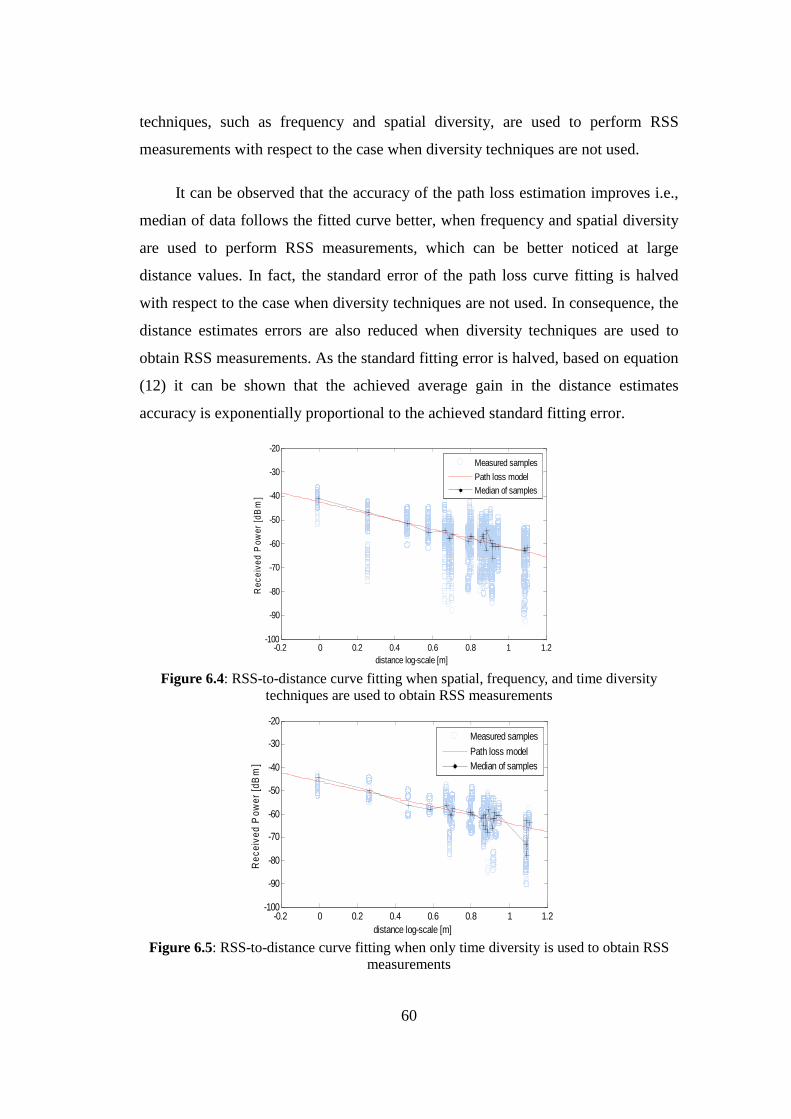
60

techniques, such as frequency and spatial diversity, are used to perform RSS

measurements with respect to the case when diversity techniques are not used.

It can be observed that the accuracy of the path loss estimation improves i.e.,

median of data follows the fitted curve better, when frequency and spatial diversity

are used to perform RSS measurements, which can be better noticed at large

distance values. In fact, the standard error of the path loss curve fitting is halved

with respect to the case when diversity techniques are not used. In consequence, the

distance estimates errors are also reduced when diversity techniques are used to

obtain RSS measurements. As the standard fitting error is halved, based on equation

(12) it can be shown that the achieved average gain in the distance estimates

accuracy is exponentially proportional to the achieved standard fitting error.

Figure 6.4: RSS-to-distance curve fitting when spatial, frequency, and time diversity

techniques are used to obtain RSS measurements

Figure 6.5: RSS-to-distance curve fitting when only time diversity is used to obtain RSS

measurements

-0.2 0 0.2 0.4 0.6 0.8 1 1.2-100

-90

-80

-70

-60

-50

-40

-30

-20

distance log-scale [m]

Rec

eive

d P

ower

[dB

m]

Measured samples

Path loss modelMedian of samples

-0.2 0 0.2 0.4 0.6 0.8 1 1.2-100

-90

-80

-70

-60

-50

-40

-30

-20

distance log-scale [m]

Rec

eive

d P

ower

[dB

m]

Measured samples

Path loss modelMedian of samples

61

6.3.2 Counteracting shadow fading

The second part of the experiment, corresponding to Figure 6.6, provides a

comparison of the accuracy of the path loss estimation when anchor-specific path

loss estimations are performed with respect to the case when a shadowing-

dependent path loss estimation is performed, i.e., RSS measurements taken at

different receivers, whose observations are affected by independent shadow fading,

are used to perform a single overall path loss estimation.

Figure 6.6 shows the standard error of the shadowing-dependent path loss

curve fitting (bar number 0) together with the standard errors of the anchor-specific

path loss curves fittings (bars number 1-7). It can be observed that the standard

error of the path loss curve fitting is on average reduced by about 25% when

anchor-specific path loss estimations are performed. In consequence, the distance

estimates errors are also reduced when anchor-specific path loss estimations are

used to deduce distances, provided that the those estimations are performed using

RSS measurements taken at a certain receiver, anchored at the perimeter of a

convex area, within a period of time when the channel is essentially invariant.

The present ranging system showed to achieve 1.25 m average accuracy on

the distance estimates. This error can be generalized in terms of the radio range, so

that the average distance estimates accuracy is about 8% of the radio range,

according to our estimation of the radio range.

Figure 6.6: Standard error of the curve fittings

0 1 2 3 4 5 6 7 0 0.5

1 1.5

2 2.5

3 3.5

4 4.5

Curve

Sta

ndar

d er

ror

[dB

]

62

6.3.3 Location estimate

In the present section we look at the accuracy of the location estimate. Here, the

actual localization accuracy of the solution may vary with the number of anchor

nodes used, the radio range, and the propagation characteristics of the environment.

In the experiment, a blind was placed at 20 different locations for finding its

location. Figure 6.7 shows the Cumulative Distribution Function (CDF) of the

absolute localization error, where the average localization error was observed to be

around 2.1 m. This error can be generalized in terms of the radio range, so that the

average localization accuracy is about 14% of the radio range according to our

estimation of the radio range. Nevertheless, propagation-based ranging may lead to

unpredictable results as shown in Figure 6.7, where localization errors about half of

the radio range can be observed.

0 1 2 3 4 5 6 7 8 9 100

0.1

0.2

0.3

0.4

0.5

0.6

0.7

0.8

0.9

1

localization error

Cum

mul

ativ

e pr

obab

ility

Figure 6.7: CDF of the absolute localization error

63

CHAPTER 7

Conclusions and Future Work

7.1 Conclusions

Acknowledging the increasing demand of many error-tolerant location-aware

applications, the present research enhances the performance of simple and low-cost

propagation-based localization solutions for wireless sensors networks in dynamic

indoor situations, where the cost and form are major concerns.

The present solution then implements practical and novel methods in order to

counteract the two major sources of distance estimates errors under the propagation-

based approach such as multipath effect and shadow fading. The use of diversity

techniques showed to halve the standard error of the estimations of the path loss, on

average, which in turn reduces the distance estimates errors. Moreover, the use of

anchor-specific path loss estimations in order to account for the independent

shadow fading affecting the observations at different anchor nodes showed to

reduce the standard error of the estimations of the path loss by about 25%, on

average, which in turn reduces the distance estimates errors. The achieved average

distance estimates accuracy is about 10% of the radio range when seven anchor

64

nodes are used.

On the other hand, the solution implements a non-constrained optimization

algorithm, such as the weighted least-squares algorithm, in order to find out blinds’

locations. This algorithm showed to reduce the impact of the distance estimates

errors on the location estimate, where the achieved gain on the distance fitting

accuracy increases as the number of beacons grows to infinity. The achieved

average localization accuracy is about 14% of the radio range when seven anchor

nodes are used. It can be concluded that propagation-based localization solutions

can lead to unpredictable results in hostile situations, apart that they are limited to

the region where the radiated power is uniform; however, they can provide

localization services to many error-tolerant applications under good situations.

7.2 Future work

It is clear that the present ranging system does counteract major problems of

distance estimation caused by the radio channel such as the multipath effect and

shadow fading, enhancing the performance of simple and low-cost propagation

based localization solutions. However, unpredictable results were observed under

hostile situations. Here, it would be interesting to determine the bounds of both

distance estimates errors and localization errors under hostile situations such as

highly scattered environments with metallic bodies and obstacles moving around.

Also, the present solution implements a non-constrained localization

algorithm; however, as discussed in Chapter 4, higher localization accuracy can be

achieved when the locations solution is constrained by the properties of the network

graph and/or additional information like for instance the expected range of the fitted

distances. Thus, it would be interesting to evaluate constrained localization

problems in order to reduce the impact of distance estimates errors on the location

estimate.

Finally, the present centralized implementation has been used in order to

validate the designed solution. However, even thought some upgrading directions of

the present solution are discussed throughout the thesis in case the solution needs to

65

support large-scale multi-hop networks, it would be interesting to asses the

improvements and challenges of a possible decentralized implementation of the

solution.

66

References

[1] N. Priyantha, A. Chakraborthy and H. Balakrishnan, “The Cricket Location-Support System,” Proceedings of International Conference on Mobile Computing and Networking, pp. 32-43, August 6-11, 2000, Boston, MA, Available online at February 02, 2010, http://nms.lcs.mit.edu/papers/cricket.html

[2] A. Savvides, C. Han, and M. B. Strivastava, “Dynamic Fine-Grained Localization

in Ad-Hoc Networks of Sensors,” Proc. MobiCom, Rome, Italy, 2001, pp. 166–79, Available online at February 02, 2010, http://portal.acm.org/citation.cfm?id=381693

[3] C.Wang and L. Xiao, “Sensor localization under limited measurement

capabilities,” IEEE Network, vol. 21, no. 3, pp. 16–23, May-June 2007, Available online at February 02, 2010, http://ieeexplore.ieee.org/xpls/abs_all.jsp?arnumber=4211213

[4] D. Lymberopoulos, Q. Lindsey, A. Savvides, “An empirical characterization of

radio signal strength variability in 3-d ieee 802.15.4 networks using monopole antennas,” (eds.) EWSN 2006, LNCS, vol. 3868, pp. 326–341, Springer, Heidelberg (2006), Available online at February 02, 2010, http://www.eng.yale.edu/enalab/publications/rssi_paper.pdf

[5] D. Moore et al., “Robust Distributed Network Localization with Noisy Range

Measurements,” Proc. SenSys, Baltimore, MD, 2004, pp. 50–61, Available online at February 02, 2010, http://rvsn.csail.mit.edu/netloc/sensys04.pdf

[6] J. Albowicz, A. Chen, and L. Zhang, “Recursive Position Estimation in Sensor

Networks,” Proc. ICNP, Riverside, CA, 2001, pp. 35–41, Available online at February 02, 2010, http://irl.cs.ucla.edu/papers/grab-icnp01.pdf

[7] Y. Shang et al., “Localization from Mere Connectivity,” Proc. MobiHoc, Annapolis,

MD, 2003, pp. 201–12, Available online at February 02, 2010, http://www.sigmobile.org/mobihoc/2003/papers/p201-shang.pdf

[8] G. Destino, and G.T.F. de Abreu, “Sensor Localization from WLS Optimization

with Closed-form Gradient and Hessian,” Center for Wireless Commun., Univ. of Oulu, Oulu, 2006-Dec, Available online at February 02, 2010, http://ieeexplore.ieee.org/xpls/abs_all.jsp?arnumber=4151125

[9] P. Biswas and Y. Ye, “Semidefinite Programming for Ad-Hoc Wireless

Localization,” Proceedings of Information Processing in Sensor Networks, pp. 46 - 53, USA, Available online at February 02, 2010, http://www.stanford.edu/~yyye/adhocn4.pdf

[10] Ubisense, http://www.ubisense.net [11] M. Tuchler, V. Schwarz, and A. Huber, “Location accuracy of an UWB localization

system in a multi-path environment,” Proc. of IEEE International Conference on

67

Ultra-Wideband (ICUWB), September 2005, Available online at February 02, 2010, http://www.fhnw.ch/technik/ime/publikationen/2005/pub_fullpaper.pdf

[12] T. He et al., “Range-Free Localization Schemes in Large Scale Sensor Networks,”

Proc. MobiCom, San Diego, CA, 2003, pp. 81–95, Available online at February 02, 2010, http://www.cs.virginia.edu/~th7c/paper/APIT_CS-2003-06.pdf

[13] C. Liu, K. Wu, and T. He, “Sensor localization with ring overlapping based on

comparison of received signal strength indicator,” IEEE Trans. on Mobile Computing, 2004, Available online at February 02, 2010, http://www-users.cs.umn.edu/~tianhe/Papers/LocalizationMASS.pdf

[14] X. Nguyen, M. I. Jordan, and B. Sinopoli, “A Kernel-Based Learning Approach to

Ad Hoc Sensor Network Localization,” ACM Trans. Sensor Networks, vol. 1, no, 1, 2005, pp. 134–52, Available online at February 02, 2010, http://portal.acm.org/citation.cfm?id=1077391.1077397

[15] P. Bahl, V. Padmanabhan, “RADAR: An In-Building RF-based User Location and

Tracking System,” Proceedings of INFOCOM 2000 Tel Aviv, Israel, March 2000, p775-84, vol. 2, Available online at February 02, 2010, http://research.microsoft.com/en-us/groups/sn-res/infocom2000.pdf

[16] D. Niculescu and B. Nath, “DV Based Positioning in Ad hoc Networks,” Journal of

Telecommunication Systems, 2003, Available online at February 02, 2010, http://www.springerlink.com/content/gt57ju03517v2076/fulltext.pdf

[17] R. Nagpal, “Organizing a Global Coordinate System from Local Information on an

Ad Hoc Sensor Network,” A.I. Memo 1666, MIT A.I. Laboratory, August 1999, Available online at February 02, 2010, http://groups.csail.mit.edu/mac/projects/amorphous/papers/ipsn-2003-v5.pdf

[18] Gabriele Di Stefano, Alberto Petricola, “A Distributed AOA Based Localization

Algorithm for Wireless Sensor Networks,” Department of Electrical and Information Engineering, University of L’Aquila, Italy, Available online at February 02, 2010, http://www.academypublisher.com/jcp/vol03/no04/jcp03040108.pdf

[19] Guoqiang Mao, Baris Fidan, Brian D.O. Anderson, “Wireless sensor network

localization techniques,” Computer Networks, Volume 51, Issue 10, 11 July 2007, pp. 2529-2553.

[20] M. Maroti et al., “Radio Interferometric Geolocation,” Proc. SenSys, San Diego,

CA, 2005, pp. 1–12, Available online at February 04, 2010, http://portal.acm.org/citation.cfm?id=1098918.1098920

[21] Ákos Lédeczi, János Sallai, Péter Völgyesi, and Ryan Thibodeaux, “Differential

Bearing Estimation for RF Tags,” EURASIP Journal on Embedded Systems, Volume 2009, Available online at February 04, 2010, http://www.hindawi.com/journals/es/2009/682183.html

[22] B. Kusy, J. Sallai, G. Balogh, A. Ledeczi, V. Protopopescu, J. Tolliver, F. DeNap,

68

and M. Parang, “Radio interferometric tracking of mobile wireless nodes,” Proc. of 5th International Conference on Mobile systems, applications and services (MobiSys), June 2007, Available online at February 16, 2010, http://graphics.stanford.edu/projects/lgl/papers/ksblptnp-ritmwt-07/ksblptnp-ritmwt-07.pdf

[23] B. Kusy, A. Ledeczi, and X. Koutsoukos, “Tracking mobile nodes using RF

Doppler shifts,” Proc. of 5th ACM International Conference on Embedded Networked Sensor Systems (SenSys), November 2007, Available online at February 16, 2010, http://portal.acm.org/citation.cfm?id=1322267

[24] Giovanni Zanca, Francesco Zorzi, Andrea Zanella and Michele Zorzi,

“Experimental comparison of RSSI-based localization algorithms for indoor wireless sensor networks,” REALWSN’08, April 1, 2008, Glasgow, United Kingdom, Available online at February 16, 2010, http://portal.acm.org/citation.cfm?id=1435473.1435475

[25] Stefano Tennina et al., “Locating ZigBee Nodes Using the TI’s CC2431 Location

Engine: A Testbed Platform and New Solutions for Positioning Estimation of WSNs in Dynamic Indoor Environments,” MELT’08, San Francisco, California, USA, September 19, 2008, Available online at February 16, 2010, http://portal.acm.org/citation.cfm?id=1410022

[26] M. Cao, B.D.O Anderson, A.S. Morse, “Localization with imprecise distance

information in sensor networks,” Proceedings of the Joint IEEE Conference on Decision and Control and European Control Conference, 2005, pp. 2829–2834, Available online at February 16, 2010, http://ieeexplore.ieee.org/xpl/freeabs_all.jsp?arnumber=1582592

[27] S. Schiffman, M. L. Reynolds, and F. W. Young, “Introduction to Multidimensional

Scaling,” Academic Press, 1981. [28] Savvides, A., Garber, W., Adlakha, S., Moses, R., and Srivastava, M. B., “On the

error characteristics of multihop node localization in ad-hoc sensor networks,” Proc. IPSN (Palo Alto, CA, April 2003), pp. 317-332, Available online at February 16, 2010, http://www.springerlink.com/content/nvhp4jw2c50qqlfj/fulltext.pdf

[29] E. Elnahrawy, X. Li, and R. P.Martin, “The limits of localization using signal

strength: a comparative study,” Proceeding of Sensor and Ad Hoc Communications and Networks, IEEE SECON, October 2004, pp. 406–414, Available online at February 16, 2010, http://paul.rutgers.edu/~eiman/elnahrawy04limits.pdf

[30] C. Savarese, K. Langendoen, and J. Rabaey, “Robust Positioning Algorithms for

Distributed Ad-Hoc Wireless Sensor Networks,” Proc. USENIX Annual Technical Conf., Monterey, CA, 2002, pp. 317–28, Available online at February 16, 2010, http://www.comp.nus.edu.sg/~bleong/geographic/related/savarese02robust.pdf

[31] H. Lim and J. C. Hou, “Localization for Anisotropic Sensor Networks,” Proc.

INFOCOM, Miami, FL, 2005, Available online at February 16, 2010, http://ieeexplore.ieee.org/xpl/freeabs_all.jsp?arnumber=1497886

69

[32] Seng-Yong Lau et al., “A measurement study of zigbee-based indoor localization systems under RF interference,” International Conference on Mobile Computing and Networking, Proceedings of the 4th ACM international workshop on Experimental evaluation and characterization, Beijing, China, 2009, pp. 35-42, Available online at February 16, 2010, http://portal.acm.org/citation.cfm?id=1614300

[33] Sungwon Yang and Hojung Cha, “An Empirical Study of Antenna Characteristics

Toward RF-based Localization for IEEE 802.15.4 Sensor Nodes,” Department of Computer Science, Yonsei University, Seodaemun-gu, Sinchon-dong 134, Seoul 120-749, Korea, Available online at February 16, 2010, http://www.springerlink.com/content/d5394x13401x6230/fulltext.pdf

[34] A. Goldsmith, “Wireless Communications,” New York, NY, USA: Cambridge

University Press, 2005. [35] System–on–chip for 2.4 GHz zigbee/IEEE 802.15.4 with location engine.

Datasheet, Texas Instruments, July 2007, Available online at February 16, 2010, http://focus.ti.com/lit/ds/symlink/cc2431.pdf

[36] N. Patwari et al., “Relative Location Estimation in Wireless Sensor Networks,”

IEEE Trans. Signal Proc., 2003, vol. 51, no. 8, pp. 2137–48. [37] Micro Hardware Manual, Sensinodes. [38] FreeRTOS, Available online at February 16, 2010, http://www.freertos.org/ [39] TinyOS community forum, Available online at February 16, 2010,

http://www.tinyos.net/ [40] Chipcon CC2420, Datasheet, Chipcon AS, 2004, Available online at February 16,

2010, http://focus.ti.com/lit/ds/symlink/cc2420.pdf [41] Sensinodes, Available at February 16, 2010, http://www.sensinode.com/ [42] Youssef Chraibi, “Localization in Wireless Sensor Networks,” KTH Signals

Sensors and Systems. Master's Degree Project, Stockholm, Sweden 2005 [43] Institute of Electrical and Electronics Engineers, Inc., IEEE Std. 802.15.4-2003,

New York: IEEE Press, 2003 [44] C. Wang and L. Xiao, “Locating Sensors in Concave Areas,” Proc. INFOCOM,

Barcelona, Catalunya, Spain, 2006, Available at February 16, 2010, http://ieeexplore.ieee.org/stamp/stamp.jsp?arnumber=04146877

[45] D.Gay, P.Levis, D.Culler and E.Brewer, nesC 1.1 Language Reference Manual,

May 2003 [46] Destino, G. and G.T.F. de Abreu, “Localization from Imperfect and Incomplete

Ranging,” Center for Wireless Commun., Univ. of Oulu, Oulu, Sept. 2006, Available at February 16, 2010,

70

http://ieeexplore.ieee.org/xpls/abs_all.jsp?arnumber=4022276 [47] David I. Chu et al., “On Least Squares Euclidean Distance Matrix Approximation

and Completion,” Available at February 16, 2010, http://www4.ncsu.edu/~mtchu/Research/Papers/distance03.pdf

[48] Yi Shang, Jing Meng, and Hongchi Shi, “A New Algorithm for Relative

Localization in Wireless Sensor Networks,” Department of Computer Science, University of Missouri-Columbia, Columbia, MO 65211, Available at February 16, 2010, http://ieeexplore.ieee.org/xpls/abs_all.jsp?arnumber=1302933

[49] Alan Bensky, “Short-range Wireless Communications: Fundamentals of RF System

Design and Application,” Second edition, Elsevier Editorial, 2004 [50] Daintree Networks Inc, “Locating ZigBee nodes using TI’s C2431 location engine

and the Daintree Networks Sensor Network Analyzer,” 2003-2008, Available at March 14, 2010, http://www.daintree.net/downloads/appnotes/appnote_016_sna_ti_locationing.pdf

[51] Jennifer Yick, Biswanath Mukherjee, Dipak Ghosal, “Wireless sensor network

survey,” Department of Computer Science, University of California, United States, Available at March 14, 2010, http://ece.ut.ac.ir/Classpages/F87/ECE637/FILES/material/Article%20WSN%20survey%202008.pdf

71

Appendix A. Matlab™ source code on the workstation %Energy measurements and additional data are pulled from the %network [DATA,Xblind,BOUNDdistance]=energy_measurements(); %The next function calculates the estimated locatio n of the blind %node(LOCATIONS) as well as the distance estimates errors and %localization errors(ERRORS) [LOCATIONS ERRORS]=localize(DATA,Xblind,BOUNDdistan ce) function [DATA,Xblind,BOUNDdistance]=energy_measurements() clear all ; try PRINT_COMMAND=70; EXIT_COMMAND=80; ERASE_MEMORY=90; %INPUT CONFIGURATION DATA %serial port communication com_number=input( 'COM PORT NUMBER: ' , 's' ); %labels the measurements round round_code=input( 'ROUND CODE: ' ); %total number of measuring nodes nodes_num=input( 'NUMBER OF NODES: ' ); %defines the measuring nodes to be localized Nblinds_=input( 'Number of blinds: ' ); %number of broadcast packets per measuring node PACKETS_NUM=input( 'NUMBER OF PACKETS TO BROADCAST: ' ); %time interval between consecutive beacons TX_int=input( 'TRANSMISSION INTERVAL [ms]: ' ); %control channel Radio_Channel=input( 'CONTROL CHANNEL [11,26]: ' ); %output power Transmission_power=input( 'TRANSMITTING POWER [0-100%]: ' ); %number of channel hops hop_num=input( 'CHANNEL HOP SEQUENCE LENGTH: ' ); %bounds the minimum value of a distance estimate BOUNDdistance_min=input( 'Minimum distance estimate [m]: ' ); %bounds the maximum value of a distance estimate BOUNDdistance_max=input( 'Maximum distance estimate [m]: ' ); %for convinience only once blind node was considere d, and its %true locations is required to compute the loca lization error blind_x=input( 'True blind location (x-axis): ' ); blind_y=input( 'True blind location (y-axis): ' ); Xblind = [blind_x,blind_y]; Nblinds=Nblinds_; BOUNDdistance.min=BOUNDdistance_min; BOUNDdistance.max=BOUNDdistance_max; nodes_number=nodes_num; PACKETS_NUMBER=PACKETS_NUM;

72

TX_interval=TX_int; Radio_Ch=Radio_Channel; TX_power=Transmission_power; Round=round_code; hop=hop_num; %channel hopping sequence for i=1:hop seq(i) = input([ 'CHANNEL ' num2str(i) ' IN HOPPING SEQUENCE: ' ]); end CONFIG.round=Round; CONFIG.num_nodes=nodes_num; CONFIG.num_packets=PACKETS_NUM; CONFIG.tx_int=TX_int; CONFIG.radio_ch=Radio_Channel; CONFIG.TX_power=Transmission_power; CONFIG.channels_to_hop=hop; CONFIG.hop_sequence=seq; AVR_RSSI_matrix=zeros(nodes_num,nodes_num); RPR_matrix=zeros(nodes_num,nodes_num); data_mat = zeros((nodes_num - 1) * PACKETS_NUM, 5); data_poll = zeros((nodes_num - 1) * PACKETS_NUM , 5); packets_numberLS=mod(PACKETS_NUMBER,255); packets_numberMS=floor(PACKETS_NUMBER/255); TX_intervalLS=mod(TX_interval,255); TX_intervalMS=floor(TX_interval/255); comstring=strcat( 'COM' ,com_number); com_port=comstring; baudrate=115200; uart_timeout=10; warning off MATLAB:serial:fscanf:unsuccessfulRead s=serial(com_port); set(s, 'BaudRate' ,baudrate); set(s, 'Timeout' ,uart_timeout); s.Flowcontrol= 'software' ; s.BytesAvailableFcnMode = 'terminator' ; disp( 'before opening port' ); fopen(s); disp( 'after opening port' ); pause(5); configuration(1)=nodes_number; configuration(2)=packets_numberLS; configuration(3)=packets_numberMS; configuration(4)=TX_intervalLS; configuration(5)=TX_intervalMS; configuration(6)=Radio_Ch; configuration(7)=TX_power;

73

configuration(8)=hop; for i=1:hop configuration(8 + i) = seq(i); end for i=1:length(configuration) fwrite(s,configuration(i), 'uint8' ); end %passing on configuration parameters to sink node TF=0; while TF~=1 out=fscanf(s); if out~=0 out end TF=strncmp(out, 'CONFIG PARAMATERS',10); end disp( 'CONFIGURATION DONE'); TF=0; while TF~=1 out=fscanf(s); if out~=0 out end TF=strncmp(out, 'MEMORY ALLOCATED',10); end disp( 'MEMORY ALLOCATION DONE'); TF=0; while TF~=1 out=fscanf(s); if out~=0 out end TF=strncmp(out, 'START APPLICATION MESSAGE' ,10); end disp( 'APPLICATION START' ); %measurments round started TF=0; while TF~=1 out=fscanf(s); if out~=0 out end TF=strncmp(out, 'ROUND COMPLETED',10); end disp( 'ROUND COMPLETED'); %measurements round ended %PULLING MEASUREMENTS FROM MEASURING NODES exit=0; while exit~=1 disp( 'NODE TO POLL?' ); disp( 'Enter the number of the node to poll:' ); disp( 'Press p to print the results of the sink node' );

74

disp( 'Press e to exit:' ); disp( 'Press r to erase memory' ); command=input( '' , 's' ); pause(1); if (command~= 'e' & command~= 'p' & command~= 'r' ) command=str2num(command); fwrite(s,command, 'uint8' ); TFprinted=0; TFresults=0; row = 1; while TFprinted~=1 out=fscanf(s); TFprinted=strncmp(out, 'POLL PRINTED' ,8); TFresults=strncmp(out, 'DATA' ,5); if TFresults out numbers=regexp(out, '(\d|[-])*' , 'match' ); node_from=str2double(char(numbe rs(1))); packet_number=str2double(char(n umbers(2))); RSSI=str2double(char(numbers(3) )); LQI=str2double(char(numbers(4)) ); noise=str2double(char(numbers(5 ))); data_poll(row,1) = node_from; data_poll(row,2) = packet_numbe r; data_poll(row,3) = RSSI; data_poll(row,4) = LQI; data_poll(row,5) = noise; row = row + 1; end end DATA{command + 1}=sortrows(data_poll,[1 2]); data_poll = zeros((nodes_num - 1) * PAC KETS_NUM, 5); disp( 'POLL PRINTED' ); elseif (command== 'p' ) fwrite(s,PRINT_COMMAND, 'uint8' ); TFprint=0; TFresults=0; line = 1; while TFprint~=1 out=fscanf(s); TFprint=strncmp(out, 'PRINT COMPLETED' ,10); TFresults=strncmp(out, 'DATA' ,5); if TFresults out

75

numbers=regexp(out, '(\d|[-])*' , 'match' ); node_from=str2double(char(numbe rs(1))); packet_number=str2double(char(n umbers(2))); RSSI=str2double(char(numbers(3) )); LQI=str2double(char(numbers(4)) ); noise=str2double(char(numbers(5 ))); data_mat(line,1) = node_from; data_mat(line,2) = packet_numbe r; data_mat(line,3) = RSSI; data_mat(line,4) = LQI; data_mat(line,5) = noise; line = line + 1; end end DATA{2}=sortrows(data_mat,[1 2]); disp( 'PRINT COMPLETED' ); elseif (command== 'r' ) disp( 'erase command' ); fwrite(s,ERASE_MEMORY, 'uint8' ); TF=0; while TF~=1 out=fscanf(s); if out~=0 out end TF=strncmp(out, 'Flash memory erased' ,10); end disp( 'Flash memory erased' ); elseif (command== 'e' ) fwrite(s,EXIT_COMMAND, 'uint8' ) TF=0; while TF~=1 out=fscanf(s); if out~=0 out end TF=strncmp(out, 'EXIT POLLING' ,10); end disp( 'EXIT POLLING' ); exit=1; end end DATA{1}=CONFIG; fclose(s); catch ME DATA{1}=CONFIG; fclose(s); end

76

function [LOCATIONS ERRORS]=localize(DATA,Xblind,BOUNDdista nce) CONFIG=DATA{1}; fullTABLE=DATA(2:end); for i=1:CONFIG.num_nodes fullTABLE{i}=sortrows(fullTABLE{i},[1 2]); end %PARAMETERS %Well-known anchors locations (true blinds location s are appended %for error calculation at the end) Xnodes =[ 0.5000 1.9600 0.5000 4.9000 5.3200 8.2600 6.3000 8.2600 12.1800 5.7400 12.1800 3.9200 5.8800 0.5000]; Xnodes=[Xblind;Xnodes]; %initial guess of blinds locations for i=1:Nblinds X0blinds(i,:) = rand(1,2).*[max(Xnodes(:,1)),ma x(Xnodes(:,2))]; end %number of measuring nodes N=CONFIG.num_nodes/2; %number of blinds Nblinds=length(X0blinds(:,1)); %reference frequency fo=2405 + 5*(CONFIG.hop_sequence(1)-11); %expected accuracy range of the distance estimates (used for %location estimation, i.e., distance fitting) alpha_m=1; %expected standard error of the received signal str ength estimates %(used for curves fittings of the path loss) alpha_dBm=3; %maximum expeceted additive noise max_additive_noise=-93; %threshold for maximum allowed channel activity interference_tresh=0.3; %Euclidean distance matrix D = pdist(Xnodes, 'euclidean' ); EDM=zeros(N); c=0; for i=1:N-1 for j=i+1:N c=c+1; EDM(i,j)=D(c); end end EDM = EDM + EDM'; %taking packet drops away TABLE=cell(1,CONFIG.num_nodes); drop=1; for i=1:CONFIG.num_nodes for j=1:(CONFIG.num_nodes-1)*CONFIG.num_packets

77

if (fullTABLE{i}(j,1)==0) drop=drop+1; else break ; end end TABLE{i}=fullTABLE{i}(drop:end,:); drop=1; end %setting channels with high activity and estimating additive noise %at each measuring node activity=zeros(1,CONFIG.channels_to_hop); num_noise_samples=zeros(1,CONFIG.channels_to_hop); NOISE=cell(1,CONFIG.num_nodes); for i=1:CONFIG.num_nodes NOISE{i}=[]; for j=1:length(TABLE{i}(:,1)) packet_num=TABLE{i}(j,2); noise=TABLE{i}(j,5); if (mod(packet_num,CONFIG.channels_to_hop)==0) hop=CONFIG.channels_to_hop; else hop=mod(packet_num,CONFIG.channels_to_h op); end num_noise_samples(hop)=num_noise_samples(ho p)+1; if (noise > max_additive_noise) activity(hop)=activity(hop)+1; else NOISE{i}=[NOISE{i},noise]; end end end node_add_noise=zeros(1,CONFIG.num_nodes); for i=1:CONFIG.num_nodes node_add_noise(i)=mean(NOISE{i}); end check_interference=ones(1,CONFIG.channels_to_hop); for i=1:CONFIG.channels_to_hop if ((activity(i)/num_noise_samples(i)) > interference_ tresh) check_interference(i)=0; end end %normalizing measurements obtained at different fre quencies with %respect to the reference frequency and filtering additive noise %out of measurements TABLEnormalized=cell(1,CONFIG.num_nodes); for i=1:CONFIG.num_nodes TABLEnormalized{i}=zeros(length(TABLE{i}(:,1)), 2); for j=1:length(TABLE{i}(:,1)) TABLEnormalized{i}(j,1)=TABLE{i}(j,1); noise=TABLE{i}(j,5); rssi=TABLE{i}(j,3); packet_num=TABLE{i}(j,2); if (mod(packet_num,CONFIG.channels_to_hop)==0) hop=CONFIG.channels_to_hop;

78

else hop=mod(packet_num,CONFIG.channels_to_h op); end f=2405 + 5*(CONFIG.hop_sequence(hop)-11); if (noise < max_additive_noise && check_interference(hop)==1) TABLEnormalized{i}(j,2)=10*log10(10^(rs si/10)-10^(node_add_noise(i)/10))-20*log10(fo/f); else TABLEnormalized{i}(j,2)=0; end end end %tagging measurements obtained from the two antenna s (having %different node-IDs) of a dual node under single node tags RSSI=[]; DISTANCE_log=[]; MEASUREMENTS=cell(1,N); c=0; for i=1:2:CONFIG.num_nodes-1 c=c+1; MEASUREMENTS{c}=[TABLEnormalized{i};TABLEnormal ized{i+1}]; MEASUREMENTS{c}=sortrows(MEASUREMENTS{c},[1]); sourceID=0; for ID=1:2:CONFIG.num_nodes-1 sourceID=sourceID+1; for j=1:length(MEASUREMENTS{c}(:,1)) if (MEASUREMENTS{c}(j,1)==ID||MEASUREMENTS{c}(j,1)==ID +1) MEASUREMENTS{c}(j,1)=sourceID; if (MEASUREMENTS{c}(j,2)~=0)

RSSI=[RSSI,MEASUREMENTS{c}(j,2)]; DISTANCE_log=[DISTANCE_log,log10(EDM(c,sourceID))];

end end end end end %separating measurements taken at different anchor nodes into %different matrices and computing the median of samples, weigt hs, %and corresponding log-distances RANGEdata=cell(1,N); for i=1:N c=0; temp=[]; count=1; for j=1:length(MEASUREMENTS{i}(:,1)) if (MEASUREMENTS{i}(j,1) > 0) sourceID=MEASUREMENTS{i}(j,1); if (L(i,sourceID)~=0) temp=[temp,MEASUREMENTS{i}(j,2)]; if (MEASUREMENTS{i}(j,2)==0) count=count+1; end if (j~=length(MEASUREMENTS{i}(:,1)))

79

if (MEASUREMENTS{i}(j+1,1)~=sourceID) c=c+1; RANGEdata{i}(1,c)=log10(EDM (i,sourceID)); temp=sort(temp); temp=temp(1:end-count); RANGEdata{i}(2,c)=median(te mp); RANGEdata{i}(3,c)=qfunc(-alpha_dBm*sqrt(length(temp))/(2*std(temp)))-qfunc(alpha_dBm*sqrt(length(temp))/(2*std(temp))); median_rssi(i,sourceID)=RAN GEdata{i}(2,c); TEMP{i,sourceID}=temp; temp=[]; count=1; end else c=c+1; RANGEdata{i}(1,c)=log10(EDM(i,s ourceID)); temp=sort(temp); temp=temp(1:end-count); RANGEdata{i}(2,c)=median(temp); RANGEdata{i}(3,c)=qfunc(-alpha_dBm*sqrt(length(temp))/(2*std(temp)))-qfunc(alpha_dBm*sqrt(length(temp))/(2*std(temp))); median_rssi(i,sourceID)=RANGEda ta{i}(2,c); TEMP{i,sourceID}=temp; end end end end end %ANCHOR-SPECIFIC PATH LOSS ESTIMATIONS NODESparameters=[(1:N)',zeros(N,3)]; temp1=[]; temp2=[]; temp3=[]; for i=1:N if (size(RANGEdata{i})>[2,2]) logDV = RANGEdata{i}(1,:); rssi_estimates = RANGEdata{i}(2,:); fitweigth = RANGEdata{i}(3,:); ok_ = isfinite(logDV) & isfinite(rssi_estim ates); if ~all( ok_ ) warning( 'GenerateMFile:IgnoringNansAndInfs' , ... 'Ignoring NaNs and Infs in data' ); end ft_ = fittype( 'poly1' ); fo_ = fitoptions( 'method' , 'LinearLeastSquares' , 'Robust' , 'On' ); set(fo_, 'Weight' ,fitweigth(ok_)); [cf_ gf_] = fit(logDV(ok_),rssi_estimates(o k_),ft_,fo_) if (gf_.rsquare<0) fo_ = fitoptions( 'method' , 'LinearLeastSquares' , 'Robust' , 'Off' ); set(fo_, 'Weight' ,fitweigth(ok_)); [cf_ gf_] = fit(logDV(ok_),rssi_estimat es(ok_),ft_,fo_) end

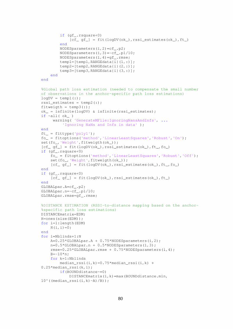
80

if (gf_.rsquare<0) [cf_ gf_] = fit(logDV(ok_),rssi_estimat es(ok_),ft_) end NODESparameters(i,2)=cf_.p2; NODESparameters(i,3)=-cf_.p1/10; NODESparameters(i,4)=gf_.rmse; temp1=[temp1,RANGEdata{i}(1,:)]; temp2=[temp2,RANGEdata{i}(2,:)]; temp3=[temp3,RANGEdata{i}(3,:)]; end end %Global path loss estimation (needed to compensate the small number of observations in the anchor-specific path loss es timations) logDV = temp1(:); rssi_estimates = temp2(:); fitweigth = temp3(:); ok_ = isfinite(logDV) & isfinite(rssi_estimates); if ~all( ok_ ) warning( 'GenerateMFile:IgnoringNansAndInfs' , ... 'Ignoring NaNs and Infs in data' ); end ft_ = fittype( 'poly1' ); fo_ = fitoptions( 'method' , 'LinearLeastSquares' , 'Robust' , 'On' ); set(fo_, 'Weight' ,fitweigth(ok_)); [cf_ gf_] = fit(logDV(ok_),rssi_estimates(ok_),ft_, fo_) if (gf_.rsquare<0) fo_ = fitoptions( 'method' , 'LinearLeastSquares' , 'Robust' , 'Off' ); set(fo_, 'Weight' ,fitweigth(ok_)); [cf_ gf_] = fit(logDV(ok_),rssi_estimates(ok_), ft_,fo_) end if (gf_.rsquare<0) [cf_ gf_] = fit(logDV(ok_),rssi_estimates(ok_), ft_) end GLOBALpar.A=cf_.p2; GLOBALpar.n=-cf_.p1/10; GLOBALpar.rmse=gf_.rmse; %DISTANCE ESTIMATION (RSSI-to-distance mapping base d on the anchor- %specific path loss estimations) DISTANCEmatrix=EDM; H=ones(size(EDM)); for i=1:length(EDM) H(i,i)=0; end for i=Nblinds+1:N A=0.25*GLOBALpar.A + 0.75*NODESparameters(i,2); n=0.5*GLOBALpar.n + 0.5*NODESparameters(i,3); rmse=0.25*GLOBALpar.rmse + 0.75*NODESparameters (i,4); B=-10*n; for k=1:Nblinds median_rssi(i,k)=0.75*median_rssi(i,k) + 0.25*median_rssi(k,i); if (BOUNDdistance~=0) DISTANCEmatrix(i,k)=max(BOUNDdistance.m in, 10^((median_rssi(i,k)-A)/B));

81

DISTANCEmatrix(i,k)=min(BOUNDdistance.m ax, DISTANCEmatrix(i,k)); else DISTANCEmatrix(i,k)=10^((median_rssi(i, k)-A)/B); end DISTANCEmatrix(k,i)=DISTANCEmatrix(i,k); %calculating weigths for distance fitting distance_samples=10.^((TEMP{i,k}-A)/B); offset=DISTANCEmatrix(i,k)*(1-exp(-(1/2)*((rmse*log(10))/(10*n))^2)); H(i,k)=qfunc(-abs(alpha_m+offset)*sqrt(length(distance_samples))/ (2*std(distance_samples)))-qfunc(abs(alpha_m-offset)*sqrt(length(distance_samples))/(2*std(dista nce_samples)));; H(k,i)=H(i,k); end end %calculating distance estimates errors temp=[]; for i=Nblinds+1:N for k=1:Nblinds distance_error=abs(EDM(i,k)-DISTANCEmatrix( i,k)); temp=[temp,distance_error]; end end RANGEerror.mean=mean(temp); RANGEerror.max=max(temp); %LOCATION ESTIMATION (weigthed least-squares optimi zation) X=Xnodes; X(1:Nblinds,:)=X0blinds; x0=[]; for i=1:N for j=1:2 x0 = [x0; X((j-1) * N + i)]; end end DISTANCEvector=DISTANCEmatrix(find(tril(ones(N),-1) ))'; H_=H(find(tril(ones(N),-1)))'; options = optimset( 'Jacobian' , 'on' ); [Xestimate,resnorm] = lsqnonlin(@(x)Jwls(x,DISTANCEvector,H_,N,2),x0,-inf*ones(N*2,1),inf*ones(N*2,1),options); LOCATIONS=zeros(N,2); for i=1:2 for j=1:N LOCATIONS(j,i) = [Xestimate((j-1) * 2 + i)] ; end end %calculating location estimate errors temp=[]; for k=1:Nblinds localization_error=pdist([LOCATIONS(k,:);Xnodes (k,:)]); temp=[temp,localization_error];

82

end LOCALIZATIONerror.mean=mean(temp); LOCALIZATIONerror.max=max(temp); ERROR(1)=RANGEerror; ERROR(2)=LOCALIZATIONerror; function [F J]= Jwls(x,D,H,N,m) Xmatrix=zeros(N,m); for i=1:m for j=1:N Xmatrix(j,i) = [x((j-1) * m + i)]; end end %calculating vector of non-redundant equations usin g the weigthed %least-squares cost function F = (H .* (D.^2 - (pdist(Xmatrix, 'euclidean' )).^2))'; %calculating the Jacobian temp1 = zeros(length(D),m*N); for v=1:N c=0; temp=zeros(length(D),m); for i=1:N for j=i+1:N c=c+1; if (v==i & v~=1:m+1) temp(c,:)=-2*H(c)*(Xmatrix(v,:)-Xma trix(j,:)); end if (v==j & v~=1:m+1) temp(c,:)=-2*H(c)*(Xmatrix(v,:)-Xma trix(i,:)); end end end temp1(:,m*v-(m-1):m*v)=temp; end J=temp1;

83

B. C-source code on the measuring node /* Created by: JS */ /* Revised by: JV */ /***** file main.c *****/ /* Standard includes. */ #include <stdlib.h> #include <signal.h> #include <string.h> /* Scheduler includes. */ #include "FreeRTOS.h" #include "task.h" #include "queue.h" #include "bus.h" #include "gpio.h" #include "debug.h" #include "socket.h" #include "rf.h" #include "buffer.h" #include "flash.h" /* tasks declaration */ static void Node( void * pvParameters ); /* Constants declaration */ uint8_t NODE_ID =3; //1 is ONLY for the sink node! uint8_t BROADCAST_PACKET =23; uint8_t START_APPLICATION =1; uint8_t POLL =40; uint8_t POLL_ANSWER =50; uint8_t ICS =200 ; // ms #define PRINT_COMMAND 70 #define ERASE_MEMORY 90 /* Variables declaration */ uint16_t PACKETS_NUMBER ; uint8_t RADIO_CHANNEL ; uint8_t TX_POWER ; uint16_t TX_interval ; uint8_t TX_intervalLS ; uint8_t TX_intervalMS ; uint8_t packets_numberLS ; uint8_t packets_numberMS ; int8_t byte ; uint8_t nodes_number ; uint16_t pac_counter ; uint8_t TX_NODE_ID ; int8_t RSSI_packet ; int8_t noise ; uint8_t not_started ; uint8_t not_polled ; uint8_t current_radio_channel ; uint8_t data [ 253 ]; // 252B + 1B = 42 packet + idx uint8_t rec_packet_counter ; uint16_t j ; uint32_t ADD ; uint32_t ADD_print ; uint16_t packet_number ; uint8_t packet_numLS ; uint8_t packet_numMS ; uint8_t last_page ; uint8_t content ;

84

uint8_t LQI_packet ; uint8_t * channel_seq ; uint8_t next ; uint8_t hop_num ; uint16_t i ; portTickType start_tx_time ; portTickType stop_tx_time ; portTickType recorded_time ; portTickType wait_tiempo ; portTickType wait_tiempo_temp ; portTickType tiempo_to_TX ; portTickType wait_to_change ; portTickType wait_to_change_temp ; portTickType time_to_change ; uint8_t distance ; uint8_t distance_to_last ; uint8_t first_reference ; uint8_t check ; /* Sockets declaration */ socket_t * Radio_Socket =0; /* Buffers declaration */ buffer_t * R_Buffer ; buffer_t * T_Buffer ; /* Ports definition */ #define BROADCAST_PORT_NUM 20 /* Addresses declaration */ sockaddr_t Broadcast_Add = {

ADDR_802_15_4_PAN_LONG, { 0xFF, 0xFF, 0xFF, 0xFF, 0xFF, 0xFF, 0xFF, 0xFF, 0xFF, 0xFF }, BROADCAST_PORT_NUM

}; /* main */ int main ( void ) {

/* Initializes the leds */ LED_INIT (); if ( bus_init () == pdFALSE) { } /* Initializes the debug window */ debug_init ( 115200 ); stack_init (); /* Creates the tasks */ xTaskCreate ( Node, "NODE", configMAXIMUM_STACK_SIZE , NULL,( tskIDLE_PRIORITY + 0),( xTaskHandle * ) NULL); /* Starts the scheduler */ vTaskStartScheduler (); return 0;

} /* Measuring node Task */ static void Node ( void * pvParameters ) {

/* wait user input */ LED2_ON(); byte = - 1;

85

debug ( "NODE WAITING FOR COMMAND\r\n" ); byte = debug_read_blocking ( 5000 ); LED2_OFF(); /*pulls measurmrnets data via serial communication when the measuring node is attached to the workstation*/ if ( byte == PRINT_COMMAND) {

last_page =0; ADD_print =0; while ( last_page != 1) {

if ( flash_read ( ADD_print , data , sizeof ( data )) == pdTRUE) {

content =data [ 0]; if ( content ==255 ) {

debug ( "PRINT COMPLETED\r\n" ); last_page =1;

} else {

for ( j =0; j <=( uint16_t )( content - 1)* 6; j =j +6) { TX_NODE_ID = data [ j +1]; packet_numLS = data [ j +2]; packet_numMS = data [ j +3]; packet_number = packet_numLS +( packet_numMS <<8); RSSI_packet = data [ j +4]; LQI_packet = data [ j +5]; noise = data [ j +6]; vTaskDelay ( 20); }

} } ADD_print =ADD_print +256 ;

} } /*erase memory*/ else if ( byte == ERASE_MEMORY) {

debug ( "Starting bulk erase\r\n" ); while ( flash_bulk_erase () != pdTRUE) {

debug ( "." ); vTaskDelay ( 10);

} debug ( "Flash memory erased\r\n" );

} // end of user input

/* ACTUAL PROGRAM FOR ENERGY MEASUREMENTS AND FOR PASSING DATA ON REQUEST*/ else {

Radio_Socket =socket ( MODULE_CUDP, 0); socket_bind ( Radio_Socket ,& Broadcast_Add ); for (;;) {

/*CONFIGURATION PHASE*/ //initial radio and memory settings rf_power_set ( RF_DEFAULT_POWER); current_radio_channel =rf_channel_set ( RF_DEFAULT_CHANNEL); while ( flash_bulk_erase () != pdTRUE)

86

{ debug ( "." ); vTaskDelay ( 10);

} /*measuring node waits configuration parameters fro m sink node*/ not_started = 1; while ( not_started ) {

R_Buffer =socket_read ( Radio_Socket , 0); if ( R_Buffer ==0) { } else {

if ( buffer_pull_uint8 ( R_Buffer ) == START_APPLICATION) {

nodes_number = buffer_pull_uint8 ( R_Buffer ); packets_numberLS = buffer_pull_uint8 ( R_Buffer ); packets_numberMS = buffer_pull_uint8 ( R_Buffer ); PACKETS_NUMBER = packets_numberLS +( packets_numberMS <<8); TX_intervalLS = buffer_pull_uint8 ( R_Buffer ); TX_intervalMS = buffer_pull_uint8 ( R_Buffer ); TX_interval = TX_intervalLS +( TX_intervalMS <<8); RADIO_CHANNEL = buffer_pull_uint8 ( R_Buffer ); TX_POWER = buffer_pull_uint8 ( R_Buffer ); hop_num = buffer_pull_uint8 ( R_Buffer ); channel_seq =( uint8_t *) malloc ( hop_num* sizeof ( uint8_t )); for ( i =0; i <hop_num; i ++) {

channel_seq [ i ]= 0; } for ( i =0; i <hop_num; i ++) {

channel_seq [ i ] = buffer_pull_uint8 ( R_Buffer ); } not_started = 0;

} socket_buffer_free ( R_Buffer ); R_Buffer =0;

} } //update radio settings current_radio_channel =rf_channel_set ( channel_seq [ 0]); rf_power_set ( TX_POWER); /*MEASUREMENTS PHASE: packet handling for the measu rments round (sink node initilizes the measurements round) */ wait_tiempo = (( nodes_number - 1) * TX_interval + ICS)/ portTICK_RATE_MS ; wait_to_change = (( nodes_number - NODE_ID) * TX_interval + ( ICS / 2))/ portTICK_RATE_MS ; j =0; ADD=0; rec_packet_counter =0; packet_number =0; pac_counter = 0; next =1; first_reference = 0; check = 0;

87

for (;;) {

if ( first_reference && pac_counter <= PACKETS_NUMBER) {

/* check if time to transmit expired*/ if ( xTaskGetTickCount () > tiempo_to_TX ) {

T_Buffer =socket_buffer_get ( Radio_Socket ); if ( T_Buffer ) {

buffer_push_uint8 ( T_Buffer , BROADCAST_PACKET); buffer_push_uint8 ( T_Buffer , NODE_ID); buffer_push_uint8 ( T_Buffer , ( pac_counter >>8)); buffer_push_uint8 ( T_Buffer , pac_counter ); if ( socket_sendto ( Radio_Socket ,& Broadcast_Add , T_Buffer ) == pdTRUE) {

T_Buffer = 0; } else {

socket_buffer_free ( T_Buffer ); T_Buffer = 0;

} } pac_counter ++; /* update time to transmit and time to change the channel*/ recorded_time = xTaskGetTickCount (); tiempo_to_TX = recorded_time + wait_tiempo ; time_to_change = recorded_time + wait_to_change ; check =1;

} /* check if time to change the channel expired*/ if ( xTaskGetTickCount () > time_to_change && hop_num > 1 && check ) {

check = 0; current_radio_channel =rf_channel_set ( channel_seq [ next]); next ++; if ( next > hop_num - 1) {

next = 0; }

} }

/* check if a beacon has been received*/ R_Buffer =socket_read ( Radio_Socket , 0); if ( R_Buffer ==0) { } else {

if ( buffer_pull_uint8 ( R_Buffer ) == BROADCAST_PACKET) {

/*for estimation of the additive noise and channel activity*/ noise = rf_analyze_rssi (); // data operations rec_packet_counter ++;

88

TX_NODE_ID = buffer_pull_uint8 ( R_Buffer ); packet_numMS = buffer_pull_uint8 ( R_Buffer ); packet_numLS = buffer_pull_uint8 ( R_Buffer ); packet_number = packet_numLS +( packet_numMS <<8); RSSI_packet = R_Buffer -> options . rf_dbm ; LQI_packet = R_Buffer -> options . rf_lqi ; if ( first_reference == 0) /*when first beacon of the measurements round is received*/ {

recorded_time = xTaskGetTickCount (); //update time to transmit if ( TX_NODE_ID < NODE_ID) {

pac_counter = packet_number ; distance = NODE_ID - TX_NODE_ID; wait_tiempo_temp = ( distance * TX_interval )/ portTICK_RATE_MS ; tiempo_to_TX = recorded_time + wait_tiempo_temp ;

} else {

pac_counter = packet_number + 1; distance = ( nodes_number + NODE_ID) - TX_NODE_ID; wait_tiempo_temp = (( distance - 1) * TX_interval + ICS)/ portTICK_RATE_MS ; tiempo_to_TX = recorded_time + wait_tiempo_temp ;

} // update time to change the channel distance_to_last = nodes_number – TX_NODE_ID; wait_to_change_temp = ( distance_to_last * TX_interval + ( ICS / 2))/ portTICK_RATE_MS ; time_to_change = recorded_time + wait_to_change_temp ; first_reference = 1; check =1;

} //data operations; data [(( rec_packet_counter - 1)* 6)+ 1]= TX_NODE_ID; data [(( rec_packet_counter - 1)* 6)+ 2]= packet_numLS ; data [(( rec_packet_counter - 1)* 6)+ 3]= packet_numMS ; data [(( rec_packet_counter - 1)* 6)+ 4]= RSSI_packet ; data [(( rec_packet_counter - 1)* 6)+ 5]= LQI_packet ; data [(( rec_packet_counter - 1)* 6)+ 6]= noise ; if ( rec_packet_counter ==42) {

data [ 0]= rec_packet_counter ; if ( flash_write ( ADD, data , sizeof ( data ))== pdTRUE) {

flash_write_wait (); } ADD=ADD+256 ; rec_packet_counter =0;

} } socket_buffer_free ( R_Buffer ); R_Buffer =0;

}

/* exit loop if the measurements round has ended*/ if ( pac_counter > PACKETS_NUMBER && ( xTaskGetTickCount () - recorded_time )* portTICK_RATE_MS > ( nodes_number -

89

NODE_ID)* TX_interval + 200 ) {

if ( rec_packet_counter != 0) {

data [ 0]= rec_packet_counter ; if ( flash_write ( ADD, data , sizeof ( data ))== pdTRUE) {

flash_write_wait (); } ADD=ADD+256 ;

} rec_packet_counter =0; break ;

} } // end of measurements phase

/* POLLING PHASE: sink node collects measurements f rom measuring nodes*/ //reset buffers and radio if ( T_Buffer ) {

socket_buffer_free ( T_Buffer ); T_Buffer = 0;

} if ( R_Buffer ) {

socket_buffer_free ( R_Buffer ); R_Buffer = 0;

} vTaskDelay ( 50); socket_close ( Radio_Socket ); Radio_Socket =socket ( MODULE_CUDP, 0); socket_bind ( Radio_Socket ,& Broadcast_Add ); current_radio_channel =rf_channel_set ( RADIO_CHANNEL); rf_power_set ( RF_DEFAULT_POWER); // waiting for poll request not_polled = 1; while ( not_polled ) {

R_Buffer =socket_read ( Radio_Socket , 5000 ); if ( R_Buffer ==0) { } else {

if ( buffer_pull_uint8 ( R_Buffer ) == POLL && buffer_pull_uint8 ( R_Buffer ) == NODE_ID) {

last_page =0; ADD_print =0 while ( last_page != 1) {

if ( flash_read ( ADD_print , data , sizeof ( data )) == pdTRUE)

{ content =data [ 0]; if ( content ==255 ) {

last_page =1; } else {

for ( j =0; j <=( uint16_t )( content - 1)* 6; j =j +6)

90

{ TX_NODE_ID = data [ j +1]; packet_numLS = data [ j +2]; packet_numMS = data [ j +3]; packet_number = packet_numLS +( packet_numMS <<8); RSSI_packet = data [ j +4]; LQI_packet = data [ j +5]; noise = data [ j +6]; T_Buffer =socket_buffer_get ( Radio_Socket ); if ( T_Buffer ) {

buffer_push_uint8 ( T_Buffer , POLL_ANSWER); buffer_push_uint8 ( T_Buffer , NODE_ID); buffer_push_uint8 ( T_Buffer , TX_NODE_ID); buffer_push_uint8 ( T_Buffer , packet_numLS ); buffer_push_uint8 ( T_Buffer , packet_numMS ); buffer_push_uint8 ( T_Buffer , RSSI_packet ); buffer_push_uint8 ( T_Buffer , LQI_packet ); buffer_push_uint8 ( T_Buffer , noise ); if ( socket_sendto ( Radio_Socket ,& Broadcast_Add, T_Buffer ) == pdTRUE) {

T_Buffer = 0; } else {

socket_buffer_free ( T_Buffer ); T_Buffer = 0;

} } vTaskDelay ( 20);

} }

} ADD_print =ADD_print +256 ;

} not_polled = 0;

} socket_buffer_free ( R_Buffer ); R_Buffer =0;

} } //end of polling phase free ( channel_seq );

} // back to configuration phase }

}

91

C. C-source code on the sink node

/* Created by: JS */ /* Revised by: JV */ /***** file main.c *****/ /* Standard includes. */ #include <stdlib.h> #include <signal.h> #include <string.h> /* Scheduler includes. */ #include "FreeRTOS.h" #include "task.h" #include "queue.h" #include "bus.h" #include "gpio.h" #include "debug.h" #include "socket.h" #include "rf.h" #include "buffer.h" #include "flash.h" #include <sys/inttypes.h> #include "control_message.h" /* tasks declaration */ static void Sink_Node ( void * pvParameters ); /* Constants declaration */ uint8_t NODE_ID =1; //1 is ONLY for the sink node! uint8_t BROADCAST_PACKET =23; uint8_t START_APPLICATION =1; uint8_t POLL =40; uint8_t POLL_ANSWER =50; uint8_t ICS =200 ; // ms #define PRINT_COMMAND 70 #define EXIT_COMMAND 80 #define ERASE_MEMORY 90 /* Variables declaration */ uint16_t PACKETS_NUMBER ; uint8_t RADIO_CHANNEL ; uint8_t TX_POWER ; uint16_t TX_interval ; uint8_t TX_intervalLS ; uint8_t TX_intervalMS ; uint8_t packets_numberLS ; uint8_t packets_numberMS ; uint8_t configuration [ 10]; uint8_t x ; uint8_t t ; uint8_t exit_condition ; int8_t byte ; uint8_t nodes_number ; uint16_t TX_pac_counter ; uint8_t TX_NODE_ID ; uint8_t node_id ; uint8_t i ; int8_t RSSI_packet ; int8_t noise ; uint8_t current_radio_channel ; int8_t data [ 253 ]; // 252B + 1B = 42 packet + idx uint8_t rec_packet_counter ;

92

uint16_t j ; uint32_t ADD ; uint32_t ADD_print ; uint16_t packet_number ; uint8_t packet_numLS ; uint8_t packet_numMS ; uint8_t last_page ; uint8_t content ; uint8_t LQI_packet ; uint16_t castMS ; uint8_t poll_completed ; uint8_t next ; uint8_t hop_num ; portTickType recorded_time ; portTickType wait_tiempo ; portTickType tiempo_to_TX ; portTickType wait_to_change ; portTickType time_to_change ; uint8_t distance ; uint8_t check ; /* Sockets declaration */ socket_t * Radio_Socket =0; /* Buffers declaration */ buffer_t * T_Buffer ; buffer_t * R_Buffer ; /* Ports definition */ #define BROADCAST_PORT_NUM 20 /* Addresses declaration */ sockaddr_t Broadcast_Add = {

ADDR_802_15_4_PAN_LONG, { 0xFF, 0xFF, 0xFF, 0xFF, 0xFF, 0xFF, 0xFF, 0xFF, 0xFF, 0xFF }, BROADCAST_PORT_NUM

}; /*function that passes on own (not collected) measu rements data to workstation*/ static void print_data ( void ) {

last_page =0; ADD_print =0; debug ( "print command received\r\n" ); while ( last_page != 1) {

if ( flash_read ( ADD_print , data , sizeof ( data )) == pdTRUE) {

content =data [ 0]; if ( content ==255 ) {

debug ( "PRINT COMPLETED\r\n" ); last_page =1;

} else {

for ( j =0; j <=( uint16_t )( content - 1)* 6; j =j +6) {

TX_NODE_ID = data [ j +1]; packet_numLS = data [ j +2]; packet_numMS = data [ j +3]; packet_number = packet_numLS +( packet_numMS <<8);

93

RSSI_packet = data [ j +4]; LQI_packet = data [ j +5]; noise = data [ j +6]; vTaskDelay ( 20);

} }

} ADD_print =ADD_print +256 ;

} } /* main */ int main ( void ) {

/* Initializes the leds */ LED_INIT (); if ( bus_init () == pdFALSE) { } /* Initializes the debug window */ debug_init ( 115200 ); stack_init (); /* Creates the tasks */ xTaskCreate ( Sink_Node , "SINKNODE", configMAXIMUM_STACK_SIZE , NULL,( tskIDLE_PRIORITY + 0),( xTaskHandle * ) NULL); /* Starts the scheduler */ vTaskStartScheduler (); return 0;

} /* Sink node Task */ static void Sink_Node ( void * pvParameters ) {

/*CONFIGURATION PHASE: sink node receives configura tion parameters from workstation and passes them on to t he network*/ LED1_ON(); vTaskDelay ( 1000 ); LED1_OFF(); for ( x=0; x<( sizeof ( configuration )); x++) {

configuration [ x] = 0; } LED2_ON(); for ( x=0; x<8; x++) //receive 7 parameters from workstation {

byte = - 1; while ( byte == - 1) {

byte = debug_read_blocking ( 1000 ); configuration [ x] = byte ;

} } LED2_OFF(); nodes_number = configuration [ 0]; packets_numberLS = configuration [ 1]; packets_numberMS = configuration [ 2]; TX_intervalLS = configuration [ 3]; TX_intervalMS = configuration [ 4]; RADIO_CHANNEL = configuration [ 5]; TX_POWER = configuration [ 6]; hop_num = configuration [ 7]; castMS = ( uint16_t ) TX_intervalMS ; TX_interval = TX_intervalLS +( castMS * 255 ); castMS = ( uint16_t ) packets_numberMS ;

94

PACKETS_NUMBER = packets_numberLS +( castMS * 255 ); debug ( "CONFIG PARAMETERS"); uint8_t * channel_seq ; channel_seq =( uint8_t *) malloc ( hop_num* sizeof ( uint8_t )); for ( i =0; i <hop_num; i ++) {

channel_seq [ i ]= 0; } debug ( "MEMORY ALLOCATED\r\n" ); LED2_ON(); for ( x=0; x<hop_num; x++) /*Receive hop_num parameters from workstation (channel hops)*/ {

byte = - 1; while ( byte == - 1) {

byte = debug_read_blocking ( 1000 ); channel_seq [ x] = byte ;

} } LED2_OFF(); while ( flash_bulk_erase () != pdTRUE) {

debug ( "." ); vTaskDelay ( 10);

} //radio settings for control channel Radio_Socket =socket ( MODULE_CUDP, 0); socket_bind ( Radio_Socket ,& Broadcast_Add ); rf_power_set ( RF_DEFAULT_POWER); current_radio_channel =rf_channel_set ( RF_DEFAULT_CHANNEL); /* Broadcast 3 START_APPLICATION packets (packet co ntains configuration parameters)*/ for ( t =1; t <=3; t ++) {

T_Buffer =socket_buffer_get ( Radio_Socket ); if ( T_Buffer ) {

buffer_push_uint8 ( T_Buffer , START_APPLICATION); buffer_push_uint8 ( T_Buffer , nodes_number ); buffer_push_uint8 ( T_Buffer , packets_numberLS ); buffer_push_uint8 ( T_Buffer , packets_numberMS ); buffer_push_uint8 ( T_Buffer , TX_intervalLS ); buffer_push_uint8 ( T_Buffer , TX_intervalMS ); buffer_push_uint8 ( T_Buffer , RADIO_CHANNEL); buffer_push_uint8 ( T_Buffer , TX_POWER); buffer_push_uint8 ( T_Buffer , hop_num); for ( x=0; x<hop_num; x++) {

buffer_push_uint8 ( T_Buffer , channel_seq [ x]); } if ( socket_sendto ( Radio_Socket ,& Broadcast_Add , T_Buffer ) == pdTRUE) { } else {

socket_buffer_free ( T_Buffer ); T_Buffer = 0;

} vTaskDelay ( 10);

} } debug ( "START APPLICATION MESSAGE TX\r\n" ); /* end of the configuration phase*/

95

/*MEASUREMENTS PHASE: sink node initiates measureme nts round*/ //reset radio for energy measurements current_radio_channel =rf_channel_set ( channel_seq [ 0]); rf_power_set ( TX_POWER); /* initialize the measurements round (sends first b eacon)*/ TX_pac_counter = 1; vTaskDelay ( 50); T_Buffer =socket_buffer_get ( Radio_Socket ); if ( T_Buffer ) {

buffer_push_uint8 ( T_Buffer , BROADCAST_PACKET); buffer_push_uint8 ( T_Buffer , NODE_ID); buffer_push_uint8 ( T_Buffer , ( TX_pac_counter >>8)); // MS buffer_push_uint8 ( T_Buffer , TX_pac_counter ); // LS if ( socket_sendto ( Radio_Socket ,& Broadcast_Add , T_Buffer ) == pdTRUE) { } else {

socket_buffer_free ( T_Buffer ); T_Buffer = 0;

} } /* packet hadling for the measurements round */ j =0; ADD=0; rec_packet_counter =0; TX_pac_counter = 2; next =1; check =1; recorded_time = xTaskGetTickCount (); last_rec = recorded_time ; wait_tiempo = (( nodes_number - 1) * TX_interval + ICS)/ portTICK_RATE_MS ; tiempo_to_TX = recorded_time + wait_tiempo ; wait_to_change = (( nodes_number - 1) * TX_interval + ICS / 2)/ portTICK_RATE_MS ; time_to_change = recorded_time + wait_to_change ; for (;;) {

// check if time to transmit expired if ( xTaskGetTickCount () > tiempo_to_TX && TX_pac_counter <= PACKETS_NUMBER) {

T_Buffer =socket_buffer_get ( Radio_Socket ); if ( T_Buffer ) {

buffer_push_uint8 ( T_Buffer , BROADCAST_PACKET); buffer_push_uint8 ( T_Buffer , NODE_ID); buffer_push_uint8 ( T_Buffer , ( TX_pac_counter >>8)); buffer_push_uint8 ( T_Buffer , TX_pac_counter ); if ( socket_sendto ( Radio_Socket ,& Broadcast_Add , T_Buffer ) == pdTRUE) {

T_Buffer = 0; } else {

socket_buffer_free ( T_Buffer ); T_Buffer = 0;

}

96

} TX_pac_counter ++; // update time to transmit recorded_time = xTaskGetTickCount (); tiempo_to_TX = recorded_time + wait_tiempo ; time_to_change = recorded_time + wait_to_change ; check =1;

} // check if time to change the channel expired if ( xTaskGetTickCount () > time_to_change && TX_pac_counter <= PACKETS_NUMBER && check && hop_num > 1) {

check =0; current_radio_channel =rf_channel_set ( channel_seq [ next ]); next ++; if ( next > hop_num - 1) {

next = 0; }

} // check if a beacon has been received R_Buffer =socket_read ( Radio_Socket , 0); if ( R_Buffer ==0) { } else {

if ( buffer_pull_uint8 ( R_Buffer ) == BROADCAST_PACKET) {

//for estimation of the additive noise and channel activity noise = rf_analyze_rssi (); // data operations rec_packet_counter ++; TX_NODE_ID = buffer_pull_uint8 ( R_Buffer ); packet_numMS = buffer_pull_uint8 ( R_Buffer ); packet_numLS = buffer_pull_uint8 ( R_Buffer ); packet_number = packet_numLS +( packet_numMS <<8); RSSI_packet = R_Buffer -> options . rf_dbm ; LQI_packet = R_Buffer -> options . rf_lqi ; data [(( rec_packet_counter - 1)* 6)+ 1]= TX_NODE_ID; data [(( rec_packet_counter - 1)* 6)+ 2]= packet_numLS ; data [(( rec_packet_counter - 1)* 6)+ 3]= packet_numMS ; data [(( rec_packet_counter - 1)* 6)+ 4]= RSSI_packet ; data [(( rec_packet_counter - 1)* 6)+ 5]= LQI_packet ; data [(( rec_packet_counter - 1)* 6)+ 6]= noise ; if ( rec_packet_counter ==42) {

data [ 0]= rec_packet_counter ; if ( flash_write ( ADD, data , sizeof ( data ))== pdTRUE) {

flash_write_wait (); } ADD=ADD+256 ; rec_packet_counter =0;

} } socket_buffer_free ( R_Buffer ); R_Buffer =0;

} // exit loop if measurements round ended if ( TX_pac_counter > PACKETS_NUMBER && ( xTaskGetTickCount () -

97

recorded_time )* portTICK_RATE_MS > ( nodes_number -NODE_ID)* TX_interval + 200 ) {

if ( rec_packet_counter != 0) {

data [ 0]= rec_packet_counter ; if ( flash_write ( ADD, data , sizeof ( data ))== pdTRUE) {

flash_write_wait (); } ADD=ADD+256 ;

} rec_packet_counter =0; break ;

} } // end of measurements phase debug ( "ROUND COMPLETED\r\n" ); /*POLLING PHASE: sink node collests measurements fr om the network*/ //reset buffers and radio if ( T_Buffer ) {

socket_buffer_free ( T_Buffer ); T_Buffer = 0;

} if ( R_Buffer ) {

socket_buffer_free ( R_Buffer ); R_Buffer = 0;

} socket_close ( Radio_Socket ); Radio_Socket =socket ( MODULE_CUDP, 0); socket_bind ( Radio_Socket ,& Broadcast_Add ); current_radio_channel =rf_channel_set ( RADIO_CHANNEL); rf_power_set ( RF_DEFAULT_POWER); /* polling procedure */ exit_condition =0; while ( exit_condition != 1) {

LED2_ON(); byte = - 1; while ( byte == - 1) {

byte = debug_read_blocking ( 1000 ); node_id = byte ;

} LED2_OFF(); switch ( byte ) {

case PRINT_COMMAND: // PRINT_COMMAND print_data (); break ;

case ERASE_MEMORY: // ERASE_MEMORY debug ( "Starting bulk erase\r\n" ); while ( flash_bulk_erase () != pdTRUE) {

debug ( "." ); vTaskDelay ( 10);

} debug ( "Flash memory erased\r\n" ); break ;

case EXIT_COMMAND: // EXIT_COMMAND

98

exit_condition =1; break ;

default : debug_printf ( "Polling node %d\r\n" , node_id ); /*Send POLL packet*/ T_Buffer =socket_buffer_get ( Radio_Socket ); if ( T_Buffer ) {

buffer_push_uint8 ( T_Buffer , POLL); buffer_push_uint8 ( T_Buffer , node_id ); if ( socket_sendto ( Radio_Socket ,& Broadcast_Add , T_Buffer ) == pdTRUE) { } else {

socket_buffer_free ( T_Buffer ); T_Buffer =0;

} } poll_completed = 0; while ( poll_completed != 1) {

R_Buffer =socket_read ( Radio_Socket , 2000 ); if ( R_Buffer ==0) {

poll_completed = 1; debug ( "POLL PRINTED\r\n" );

} else {

if ( buffer_pull_uint8 ( R_Buffer ) == POLL_ANSWER) {

TX_NODE_ID = buffer_pull_uint8 ( R_Buffer ); if ( TX_NODE_ID == node_id ) {

TX_NODE_ID = buffer_pull_uint8 ( R_Buffer ); packet_numLS = buffer_pull_uint8 ( R_Buffer ); packet_numMS = buffer_pull_uint8 ( R_Buffer ); packet_number = packet_numLS +( packet_numMS <<8); RSSI_packet = buffer_pull_uint8 ( R_Buffer ); LQI_packet = buffer_pull_uint8 ( R_Buffer ); noise = buffer_pull_uint8 ( R_Buffer );

} } socket_buffer_free ( R_Buffer ); R_Buffer =0;

} } break ;

} } // end of polling phase and back to configuration p hase free ( channel_seq ); debug ( "EXIT POLLING\r\n" );

}