Acta Oceanol. Sin., 2012, Vol. 31, No. 1, P. 16-23

DOI: 10.1007/s13131-012-0171-6

http://www.hyxb.org.cn

E-mail: hyxbe@263.net

Effects of horizontal mixing on the upper ocean temperature

in the equatorial Pacific Ocean

HUANG Chuanjiang1, QIAO Fangli1∗

1 First Institute of Oceanography, State Oceanic Administration, Qingdao 266061, China

Received 19 May 2010; accepted 5 March 2011

©The Chinese Society of Oceanography and Springer-Verlag Berlin Heidelberg 2012

AbstractThe influence of horizontal mixing on the thermal structure of the equatorial Pacific Ocean isexamined based on a sigma coordinate model. In general, the distributions of the temperatureand currents simulated by the sigma coordinate model are very close to the climatology. However,the simulated thermocline along the equator is slightly diffusive so that there is a cold bias abovethe main thermocline, while there is a warm bias under the main thermocline. Both horizontaldiffusivity and viscosity have important effects on the upper thermal structure in the equatorialPacific Ocean, while their detailed dynamics are different. Horizontal diffusivity affects the thermalstructure in the upper ocean mainly through regulating the vertical diffusivity, while the horizontalviscosity does mainly through regulating directly the circulate system. A large horizontal diffusivityor a small horizontal viscosity can be in favor of simulating a more realistically thermal structurein the equatorial Pacific Ocean.

Key words: horizontal mixing, thermal structure, equatorial Pacific Ocean

1 Introduction

Ocean general circulation models (OGCMs) arewell known to be sensitively dependent on parameter-izations of subgrid scale processes. Much attention hasbeen paid to vertical mixing during the last decadesdue to its strong impacts on the density structure andthe meridional overturning circulation (Bryan, 1987),while horizontal mixing (including the horizontal diffu-sivity and the horizontal viscosity) has generally beengiven the least attention. Many models run with thesmallest horizontal mixing to prevent numerical insta-bility.

In fact, horizontal mixing processes have also sig-nificant effects on the behavior of the OGCMs. Theocean is a complicated dynamical system so that therehas a significant nonlinear interaction between hori-zontal and vertical mixing (Maes et al., 1997; Pezziand Richards, 2003), then the horizontal mixing canaffect the oceanic circulation and the climate systemvia regulating the vertical mixing. On the other hand,the horizontal mixing can directly affect the large-scale currents and mesoscale activity through regulat-ing friction in the ocean.

Both vertical mixing and circulation system playa critical role in determining the temperature struc-ture of the equatorial oceans. The equatorial PacificOcean plays an important role in the global climateand its variability due to its strong interannual anddecadal variabilities. Stockdale et al. (1993) analyzedseveral different OGCMs, and suggested that the seasurface temperature (SST) is sensitive to the horizon-tal viscosity in the equatorial Pacific Ocean. Pezzi andRichards (2003) argued that the horizontal mixing canaffect the SST of the cold tongue area through adjust-ing tropical instability waves.

However, these results were in contradiction tothose by other studies. Maes et al. (1997) investi-gated the sensitivity of the equatorial Pacific Oceanto the horizontal mixing with an OGCM, in whichthese mixing coefficients varied in three orders of mag-nitude. They argued that the horizontal mixing coeffi-cients have important effects on the Equatorial Under-current (EUC), while their effect on the SST is smallalthough there have strong nonlinear interactions be-tween the horizontal and vertical mixing. Megann andNew (2001) obtained similar results in their cases withhigh resolutions based on an isopycnal-coordinate

Foundation item: The National Natural Science Foundation of China under contract Nos 40806017 and 40730842; the NationalBasic Research Program (973 Program) of China under contract No. 2010CB950500.

∗Corresponding author, E-mail: qiaofl@fio.org.cn

1

HUANG Chuanjiang et al. Acta Oceanol. Sin., 2012, Vol. 31, No. 1, P. 16-23 17

OGCM, in which the SST and the temperature in theupper ocean were almost independent of the horizon-tal viscosity.

The sigma coordinate models traditionally usedfor coastal and regional simulations have been widelyused for basin and global scale simulations (e.g., Ezer,1999; Ezer and Mellor, 2000; Qiao et al., 2004). Inthis study, the impact of the horizontal mixing on thethermal structure in the equatorial Pacific Ocean isexamined on the basis of a sigma coordinate model.Moreover, the ability of a sigma coordinate model sim-ulating the equatorial Pacific Ocean is verified. Themodel details are discussed in Section 2. Numericalexperiments were carried out, and the results of theseexperiments are discussed in Section 3. The conclu-sions are drawn in Section 4.

2 Model linkage

The Princeton ocean model (POM, Blumberg andMellor, 1987) based on a sigma coordinate in thevertical direction is used in this study. The modeldomain covers the Pacific Ocean within 30◦S–58◦Nand 122◦E–70◦W, with a zonal resolution of 1◦. Themeridional resolution is 0.25◦ within the 10◦S–10◦Nband, and increases linearly to 1◦ by 20◦N (20◦S). Themodel has 32 layers in the vertical direction, and atleast five layers are in the top 50 m. The topographyis taken from ETOPO5, and the maximal water depthis set as 5 000 m.

The model is initiated with the temperature andsalinity conditions in January taken from the WOA01climatology (Conkright et al., 2002). The climato-logical monthly mean wind stress is taken from theQuickSCAT/NCEP blended ocean winds (Milliff et al.,2004). The surface heat and fresh water fluxes aretaken from the monthly mean climatology (da Silvaet al., 1994). Moreover, to keep surface density val-ues from drifting too far from reality, the SST and thesalinity are relaxed to the monthly mean climatology(Conkright et al., 2002), with a relaxation scale of 50W/(m2 K) for the SST and 120 d for the SSS (fora mixed layer 50 m thick). Sponge layers are placedalong the northern and southern boundaries with fiverows of grids, in which both temperature and salinityare relaxed toward the WOA01 monthly mean clima-tology.

The vertical viscosity and diffusivity are calcu-lated from the level 2.5 turbulence closure scheme(Mellor and Yamada, 1982), with background coef-

ficients of 10−4 m2/s and 10−5 m2/s, respectively. Atime-splitting scheme is used with a barotropic timestep of 60 s, and a baroclinic time step of 1 200 s,respectively.

3 Model results

In POM, the horizontal viscosity and diffusiv-ity are calculated by a Smagorinsky type formula(Smagorinsky, 1963):

(Am, Ah) = (α, β)ΔxΔy[(∂u

∂x

)2

+12

(∂v

∂x+

∂u

∂y

)2

+

(∂v

∂y

)2]1/2

,

where α and β are dimensionless adjustable parame-ters; and Δx and Δy are zonal and meridional gridintervals. In this scheme, the horizontal viscosity Am

and diffusivity Ah can vary with grid sizes and ve-locity gradients, whose values are enhanced in regionsof large grid sizes and velocity gradients. Thus it iswidely used in OGCMs with irregular grids.

Through adjusting the parameters α and β, fiveexperiments were conducted in this study (Table 1).Experiment A is a control run with α=0.2 and β=0.1,which is used to examine the ability of POM in simu-lating the equatorial Pacific Ocean. In order to exam-ine the effect of the horizontal diffusivity and viscosity,other four numerical experiments were run. Experi-ments B1 and B2 have the same α but different β withvalues of 0.05 and 0.2, respectively. In Experiments C1and C2, β is fixed but α is 0.1 and 0.4, respectively. Inorder to simulate a realistic EUC, the minimum hori-zontal viscosity is set to 1 000 m2/s within 10◦S and10◦N (Pezzi and Richards, 2003). These experimentswere spun up 12 a, and the results in the last year wereused in the following discussion.

Table 1. The Smagorinsky parameters α and β used in

experiments

Experiment

A B1 B2 C1 C2

α 0.2 0.2 0.2 0.1 0.4

β 0.1 0.05 0.2 0.1 0.1

3.1 Control run

The ability of a sigma coordinate model in sim-ulating the equatorial Pacific Ocean is studied in thissection. Figure 1 shows the annual mean sea surfacetemperature difference of Experiment A against theWOA01 climatology (Conkright et al., 2002). Exper-iment A produces a cold SST in the eastern-central

18 HUANG Chuanjiang et al. Acta Oceanol. Sin., 2012, Vol. 31, No. 1, P. 16-23

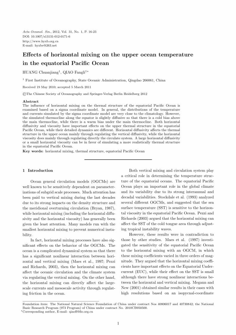
equatorial Pacific Ocean with a bias of 0.4◦C due toexcessive upward advection of cold water there, whilethe simulated SST is too warm with a bias of 0.8◦C inthe western equatorial Pacific Ocean. This SST biaspattern is quite common in most of OGCMs (Stock-dale et al., 1998). There have obvious cold biases offthe coast of South America, which is mainly associ-ated with strong northward currents.

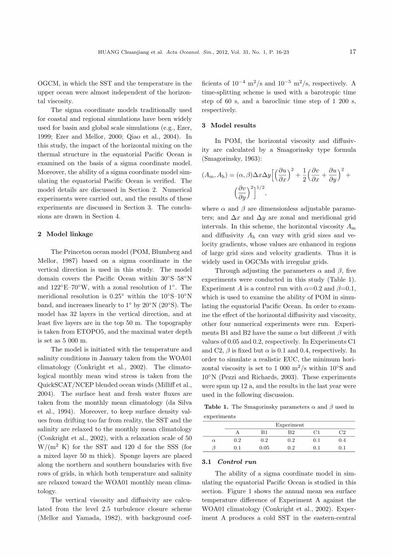
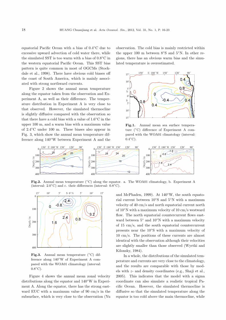
Figure 2 shows the annual mean temperaturealong the equator taken from the observation and Ex-periment A, as well as their difference. The temper-ature distribution in Experiment A is very close tothat observed. However, the simulated thermoclineis slightly diffusive compared with the observation sothat there have a cold bias with a value of 1.6◦C in theupper 100 m, and a warm bias with a maximum valueof 2.4◦C under 100 m. These biases also appear inFig. 3, which show the annual mean temperature dif-ference along 140◦W between Experiment A and the

observation. The cold bias is mainly restricted withinthe upper 100 m between 8◦S and 5◦N. In other re-gions, there has an obvious warm bias and the simu-lated temperature is overestimated.

Fig.1. Annual mean sea surface tempera-

ture (◦C) difference of Experiment A com-

pared with the WOA01 climatology (interval:

0.4◦C).

Fig.2. Annual mean temperature (◦C) along the equator. a. The WOA01 climatology, b. Experiment A(interval: 2.0◦C) and c. their differences (interval: 0.8◦C).

Fig.3. Annual mean temperature (◦C) dif-

ference along 140◦W of Experiment A com-

pared with the WOA01 climatology (interval:

0.8◦C).

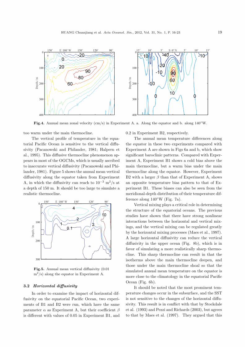
Figure 4 shows the annual mean zonal velocitydistributions along the equator and 140◦W in Experi-ment A. Along the equator, there has the strong east-ward EUC with a maximum value of 90 cm/s in thesubsurface, which is very close to the observation (Yu

and McPhaden, 1999). At 140◦W, the south equato-rial current between 10◦S and 5◦N with a maximumvelocity of 40 cm/s and north equatorial current northof 10◦N with a maximum velocity of 10 cm/s westwardflow. The north equatorial countercurrent flows east-ward between 5◦ and 10◦N with a maximum velocityof 15 cm/s, and the south equatorial countercurrentpresents near the 10◦S with a maximum velocity of10 cm/s. The positions of these currents are almostidentical with the observation although their velocitiesare slightly smaller than those observed (Wyrtki andKilonsky, 1984).

In a whole, the distributions of the simulated tem-perature and currents are very close to the climatology,and the results are comparable with those by mod-els with z- and density coordinates (e.g., Shaji et al.,2005). This indicates that the model with a sigmacoordinate can also simulate a realistic tropical Pa-cific Ocean. However, the simulated thermocline isdiffusive so that the simulated temperature along theequator is too cold above the main thermocline, while

HUANG Chuanjiang et al. Acta Oceanol. Sin., 2012, Vol. 31, No. 1, P. 16-23 19

Fig.4. Annual mean zonal velocity (cm/s) in Experiment A. a. Along the equator and b. along 140◦W.

too warm under the main thermocline.The vertical profile of temperature in the equa-

torial Pacific Ocean is sensitive to the vertical diffu-sivity (Pacanowski and Philander, 1981; Halpern etal., 1995). This diffusive thermocline phenomenon ap-pears in most of the OGCMs, which is usually ascribedto inaccurate vertical diffusivity (Pacanowski and Phi-lander, 1981). Figure 5 shows the annual mean verticaldiffusivity along the equator taken from ExperimentA, in which the diffusivity can reach to 10−3 m2/s ata depth of 150 m. It should be too large to simulate arealistic thermocline.

Fig.5. Annual mean vertical diffusivity (0.01

m2/s) along the equator in Experiment A.

3.2 Horizontal diffusivity

In order to examine the impact of horizontal dif-fusivity on the equatorial Pacific Ocean, two experi-ments of B1 and B2 were run, which have the sameparameter α as Experiment A, but their coefficient β

is different with values of 0.05 in Experiment B1, and

0.2 in Experiment B2, respectively.The annual mean temperature differences along

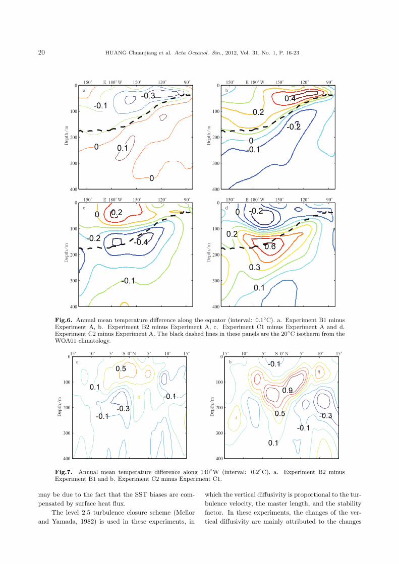
the equator in these two experiments compared withExperiment A are shown in Figs 6a and b, which showsignificant baroclinic patterns. Compared with Exper-iment A, Experiment B1 shows a cold bias above themain thermocline, but a warm bias under the mainthermocline along the equator. However, ExperimentB2 with a larger β than that of Experiment A, showsan opposite temperature bias pattern to that of Ex-periment B1. These biases can also be seen from themeridional-depth distribution of their temperature dif-ference along 140◦W (Fig. 7a).

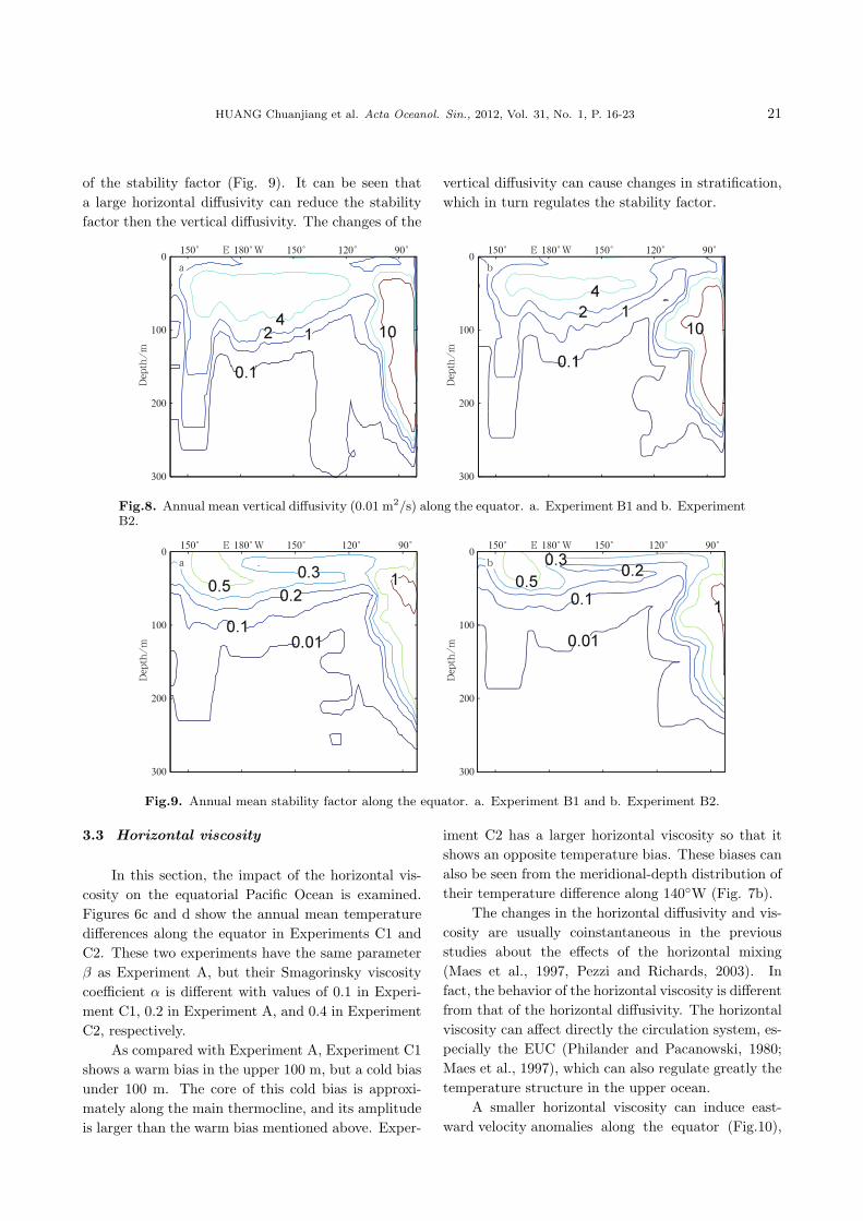
Vertical mixing plays a critical role in determiningthe structure of the equatorial oceans. The previousstudies have shown that there have strong nonlinearinteractions between the horizontal and vertical mix-ings, and the vertical mixing can be regulated greatlyby the horizontal mixing processes (Maes et al., 1997).A large horizontal diffusivity can reduce the verticaldiffusivity in the upper ocean (Fig. 8b), which is infavor of simulating a more realistically sharp thermo-cline. This sharp thermocline can result in that theisotherms above the main thermocline deepen, andthose under the main thermocline shoal so that thesimulated annual mean temperature on the equator ismore close to the climatology in the equatorial PacificOcean (Fig. 6b).

It should be noted that the most prominent tem-perature changes occur in the subsurface, and the SSTis not sensitive to the changes of the horizontal diffu-sivity. This result is in conflict with that by Stockdaleet al. (1993) and Pezzi and Richards (2003), but agreesto that by Maes et al. (1997). They argued that this

20 HUANG Chuanjiang et al. Acta Oceanol. Sin., 2012, Vol. 31, No. 1, P. 16-23

Fig.6. Annual mean temperature difference along the equator (interval: 0.1◦C). a. Experiment B1 minusExperiment A, b. Experiment B2 minus Experiment A, c. Experiment C1 minus Experiment A and d.Experiment C2 minus Experiment A. The black dashed lines in these panels are the 20◦C isotherm from theWOA01 climatology.

Fig.7. Annual mean temperature difference along 140◦W (interval: 0.2◦C). a. Experiment B2 minusExperiment B1 and b. Experiment C2 minus Experiment C1.

may be due to the fact that the SST biases are com-pensated by surface heat flux.

The level 2.5 turbulence closure scheme (Mellorand Yamada, 1982) is used in these experiments, in

which the vertical diffusivity is proportional to the tur-bulence velocity, the master length, and the stabilityfactor. In these experiments, the changes of the ver-tical diffusivity are mainly attributed to the changes

HUANG Chuanjiang et al. Acta Oceanol. Sin., 2012, Vol. 31, No. 1, P. 16-23 21

of the stability factor (Fig. 9). It can be seen thata large horizontal diffusivity can reduce the stabilityfactor then the vertical diffusivity. The changes of the

vertical diffusivity can cause changes in stratification,which in turn regulates the stability factor.

Fig.8. Annual mean vertical diffusivity (0.01 m2/s) along the equator. a. Experiment B1 and b. ExperimentB2.

Fig.9. Annual mean stability factor along the equator. a. Experiment B1 and b. Experiment B2.

3.3 Horizontal viscosity

In this section, the impact of the horizontal vis-cosity on the equatorial Pacific Ocean is examined.Figures 6c and d show the annual mean temperaturedifferences along the equator in Experiments C1 andC2. These two experiments have the same parameterβ as Experiment A, but their Smagorinsky viscositycoefficient α is different with values of 0.1 in Experi-ment C1, 0.2 in Experiment A, and 0.4 in ExperimentC2, respectively.

As compared with Experiment A, Experiment C1shows a warm bias in the upper 100 m, but a cold biasunder 100 m. The core of this cold bias is approxi-mately along the main thermocline, and its amplitudeis larger than the warm bias mentioned above. Exper-

iment C2 has a larger horizontal viscosity so that itshows an opposite temperature bias. These biases canalso be seen from the meridional-depth distribution oftheir temperature difference along 140◦W (Fig. 7b).

The changes in the horizontal diffusivity and vis-cosity are usually coinstantaneous in the previousstudies about the effects of the horizontal mixing(Maes et al., 1997, Pezzi and Richards, 2003). Infact, the behavior of the horizontal viscosity is differentfrom that of the horizontal diffusivity. The horizontalviscosity can affect directly the circulation system, es-pecially the EUC (Philander and Pacanowski, 1980;Maes et al., 1997), which can also regulate greatly thetemperature structure in the upper ocean.

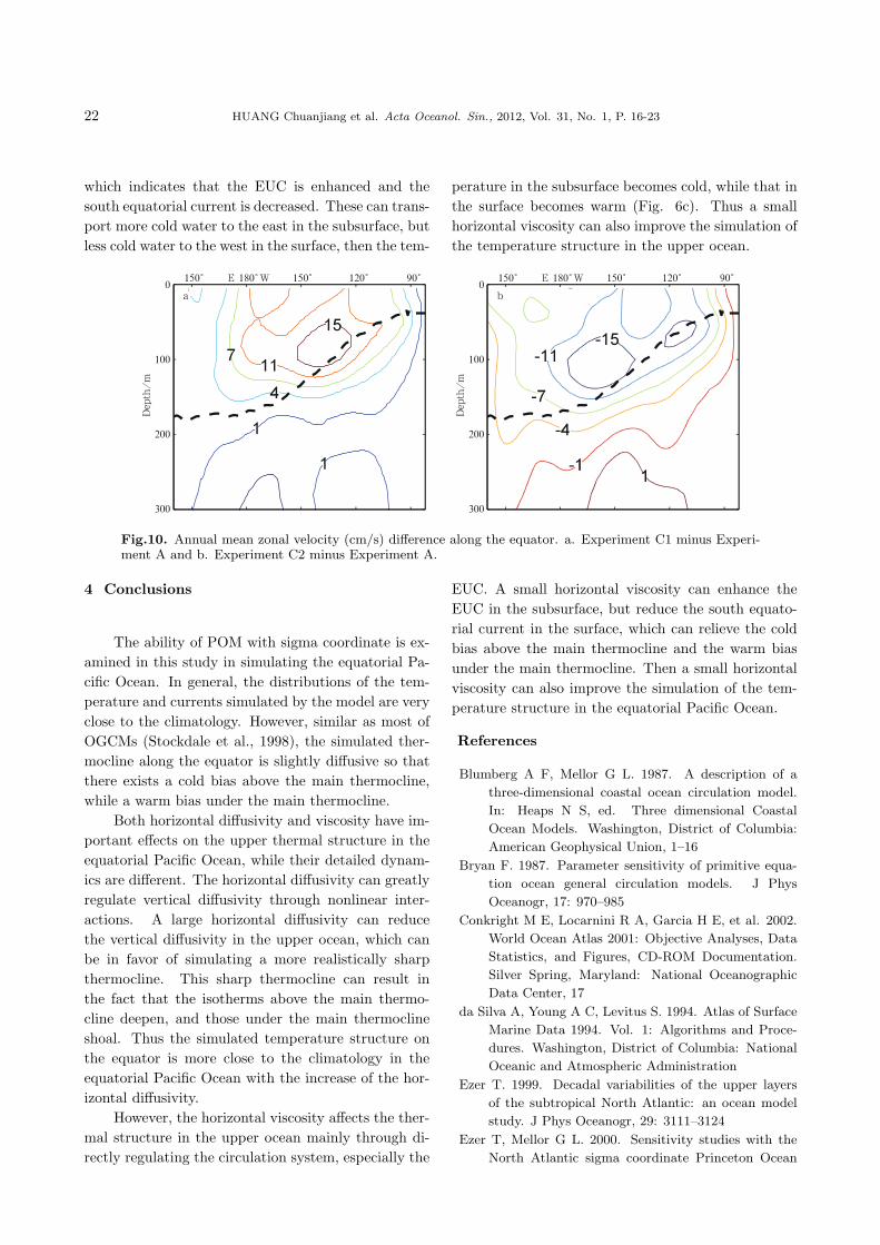
A smaller horizontal viscosity can induce east-ward velocity anomalies along the equator (Fig.10),

22 HUANG Chuanjiang et al. Acta Oceanol. Sin., 2012, Vol. 31, No. 1, P. 16-23

which indicates that the EUC is enhanced and thesouth equatorial current is decreased. These can trans-port more cold water to the east in the subsurface, butless cold water to the west in the surface, then the tem-

perature in the subsurface becomes cold, while that inthe surface becomes warm (Fig. 6c). Thus a smallhorizontal viscosity can also improve the simulation ofthe temperature structure in the upper ocean.

Fig.10. Annual mean zonal velocity (cm/s) difference along the equator. a. Experiment C1 minus Experi-ment A and b. Experiment C2 minus Experiment A.

4 Conclusions

The ability of POM with sigma coordinate is ex-amined in this study in simulating the equatorial Pa-cific Ocean. In general, the distributions of the tem-perature and currents simulated by the model are veryclose to the climatology. However, similar as most ofOGCMs (Stockdale et al., 1998), the simulated ther-mocline along the equator is slightly diffusive so thatthere exists a cold bias above the main thermocline,while a warm bias under the main thermocline.

Both horizontal diffusivity and viscosity have im-portant effects on the upper thermal structure in theequatorial Pacific Ocean, while their detailed dynam-ics are different. The horizontal diffusivity can greatlyregulate vertical diffusivity through nonlinear inter-actions. A large horizontal diffusivity can reducethe vertical diffusivity in the upper ocean, which canbe in favor of simulating a more realistically sharpthermocline. This sharp thermocline can result inthe fact that the isotherms above the main thermo-cline deepen, and those under the main thermoclineshoal. Thus the simulated temperature structure onthe equator is more close to the climatology in theequatorial Pacific Ocean with the increase of the hor-izontal diffusivity.

However, the horizontal viscosity affects the ther-mal structure in the upper ocean mainly through di-rectly regulating the circulation system, especially the

EUC. A small horizontal viscosity can enhance theEUC in the subsurface, but reduce the south equato-rial current in the surface, which can relieve the coldbias above the main thermocline and the warm biasunder the main thermocline. Then a small horizontalviscosity can also improve the simulation of the tem-perature structure in the equatorial Pacific Ocean.

References

Blumberg A F, Mellor G L. 1987. A description of a

three-dimensional coastal ocean circulation model.

In: Heaps N S, ed. Three dimensional Coastal

Ocean Models. Washington, District of Columbia:

American Geophysical Union, 1–16

Bryan F. 1987. Parameter sensitivity of primitive equa-

tion ocean general circulation models. J Phys

Oceanogr, 17: 970–985

Conkright M E, Locarnini R A, Garcia H E, et al. 2002.

World Ocean Atlas 2001: Objective Analyses, Data

Statistics, and Figures, CD-ROM Documentation.

Silver Spring, Maryland: National Oceanographic

Data Center, 17

da Silva A, Young A C, Levitus S. 1994. Atlas of Surface

Marine Data 1994. Vol. 1: Algorithms and Proce-

dures. Washington, District of Columbia: National

Oceanic and Atmospheric Administration

Ezer T. 1999. Decadal variabilities of the upper layers

of the subtropical North Atlantic: an ocean model

study. J Phys Oceanogr, 29: 3111–3124

Ezer T, Mellor G L. 2000. Sensitivity studies with the

North Atlantic sigma coordinate Princeton Ocean

HUANG Chuanjiang et al. Acta Oceanol. Sin., 2012, Vol. 31, No. 1, P. 16-23 23

Model. Dynamics of Atmospheres and Oceans, 32:

185–208

Halpern D, Chao Y, Ma C C, et al. 1995. Comparison

of tropical Pacific temperature and current simula-

tions with two vertical mixing schemes embedded in

an ocean general circulation model and reference to

observations. J Geophys Res, 100: 2515–2522

Maes C, Mades G, Delecluse P. 1997. Sensitivity of an

equatorial Pacific OGCM to the lateral diffusion.

Mon Wea Rev, 125: 958–971

Megann A, New A. 2001. The effects of resolution and

viscosity in an isopycnal-coordinate model of the

equatorial Pacific. J Phys Oceanogr, 31: 1993–2018

Mellor G L, Yamada T. 1982. Development of a turbu-

lence closure model for geophysical fluid problems.

Rev Geophys, 20: 851–875

Milliff R F, Morzel J, Chelton D B, et al. 2004. Wind

Stress Curl and Wind Stress Divergence Biases from

Rain Effects on QSCAT Surface Wind Retrievals. J

Atmos Ocean Tech, 21: 1216–1231

Pacanowski R C, Philander S G H. 1981. Parameter-

ization of vertical mixing in numerical models of

tropical oceans. J Phys Oceanogr, 11: 1443–1451

Pezzi L P, Richards K J. 2003. Effects of lateral mixing

on the mean state and eddy activity of an equato-

rial ocean. J Geophys Res, 108(C12): 3371, doi:

10.1029/2003JC001834

Philander S G H, Pacanowski R C. 1980. The generation

of equatorial currents. J Geophys Res, 85: 1123–

1136

Qiao F, Yuan Y, Yang Y, et al. 2004. Wave-induced

mixing in the upper ocean: Distribution and appli-

cation to a global ocean circulation model. Geophys

Res Lett, 31: L11303, doi: 10.1029/2004GL019824

Shaji C, Wang C, Halliwell Jr G R, et al. 2005. Simu-

lation of tropical Pacific and Atlantic Oceans using

a hybrid coordinate ocean model. Ocean Modelling,

9: 253–282

Smagorinsky J. 1963. General circulation experiments

with the primitive equations: I. The basic experi-

ment. Mon Wea Rev, 91: 99–164

Stockdale T N, Anderson D, Davey M, et al. 1993. In-

tercomparison of tropical ocean GCMs. Geneva,

Switzerland: World Climate Research Programme,

43

Stockdale T N, Busalacchi A J, Harrison D E, et al.

1998. Ocean modeling for ENSO. J Geophys Res,

103: 14325–14355

Wyrtki K, Kilonsky B. 1984. Mean water and current

structure during the Hawaii-to-Tahiti shuttle exper-

iment. J Phys Oceanogr, 14: 242–254

Yu X, McPhaden M J. 1999. Seasonal variability in the

equatorial Pacific. J Phys Oceanogr, 29: 925–947