equatorial circulation of a global ocean climate model

518 VOLUME 31J O U R N A L O F P H Y S I C A L O C E A N O G R A P H Y

q 2001 American Meteorological Society

Equatorial Circulation of a Global Ocean Climate Model withAnisotropic Horizontal Viscosity

WILLIAM G. LARGE, GOKHAN DANABASOGLU, JAMES C. MCWILLIAMS, PETER R. GENT, AND

FRANK O. BRYAN

National Center for Atmospheric Research, Boulder, Colorado

(Manuscript received 6 August 1999, in final form 3 May 2000)

ABSTRACT

Horizontal momentum flux in a global ocean climate model is formulated as an anisotropic viscosity withtwo spatially varying coefficients. This friction can be made purely dissipative, does not produce unphysicaltorques, and satisfies the symmetry conditions required of the Reynolds stress tensor. The two primary designcriteria are to have viscosity at values appropriate for the parameterization of missing mesoscale eddies whereverpossible and to use other values only where required by the numerics. These other viscosities control numericalnoise from advection and generate western boundary currents that are wide enough to be resolved by the coarsegrid of the model. Noise on the model gridscale is tolerated provided its amplitude is less than about 0.05 cms21. Parameter tuning is minimized by applying physical and numerical principles. The potential value of thisline of model development is demonstrated by comparison with equatorial ocean observations.

In particular, the goal of producing model equatorial ocean currents comparable to observations was achievedin the Pacific Ocean. The Equatorial Undercurrent reaches a maximum magnitude of nearly 100 cm s21 in theannual mean. Also, the spatial distribution of near-surface currents compares favorably with observations fromthe Global Drifter Program. The exceptions are off the equator; in the model the North Equatorial Countercurrentis improved, but still too weak, and the northward flow along the coast of South America may be too shallow.Equatorial Pacific upwelling has a realistic pattern and its magnitude is of the same order as diagnostic modelestimates. The necessary ingredients to achieve these results are wind forcing based on satellite scatterometry,a background vertical viscosity no greater than about 1 cm2 s21, and a mesoscale eddy viscosity of order 1000m2 s21 acting on meridional shear of zonal momentum. Model resolution is not critical, provided these threeelements remain unaltered. Thus, if the scatterometer winds are accurate, the model results are consistent withobservational estimates of these two coefficients. These winds have larger westward stress than NCEP reanalysiswinds, produce a 14% stronger EUC, more upwelling, but a weaker westward surface flow.

In the Indian Ocean the seasonal cycle of equatorial currents does not appear to be overly attenuated by thehorizontal viscosity, with differences from observations attributable to interannual variability. However, in theAtlantic, the numerics still require too large a meridional viscosity over too much of the basin, and a zonalresolution approaching 18 may be necessary to match observations. Because of this viscosity, increasing thebackground vertical viscosity slowed the westward surface current; opposite to the response in the Pacific.

1. Introduction

Equatorial ocean regions play a fundamental role inthe earth’s climate. In the tropical Atlantic, climate var-iability, including precipitation in adjacent continentalregions, has been related to the hemispheric gradient insea surface temperature (SST) (Hastenrath 1991; Cartonet al. 1996). The Asian–Australian monsoon has beenfound to affect global as well as regional climate onseasonal timescales, with suggestions of a role for Indianand Pacific equatorial SST (Webster et al. 1998). Ofcourse, the strongest and most predictable feature of

Corresponding author address: Dr. William G. Large, NCAR, P.O.Box 3000, Boulder, CO 80307.E-mail: [email protected].

interannual climate variability is the El Nino–SouthernOscillation (ENSO) phenomenon that is characterizedby SST anomalies in the central and eastern equatorialPacific. Describing the time-varying tropical PacificOcean, understanding the physical mechanisms ofENSO, and determining the associated predictabilitywere among the objectives of the Tropical Ocean–Glob-al Atmosphere (TOGA) program. The success of TOGAis documented in a series of review papers in a 1998special issue of the Journal of Geophysical Research(Vol. 103, No. C7). An earlier view of ENSO and otherfeatures of equatorial air–sea interaction are compre-hensively discussed in Philander (1990).

Many investigations of these phenomena rely onocean general circulation models (Stockdale et al. 1998),which are sometimes coupled to an atmosphere (Dele-cluse et al. 1998; Biasutti and Battisti 2001). For process

FEBRUARY 2001 519L A R G E E T A L .

studies (e.g., Chen et al. 1994a) and prediction purposes(Latif et al. 1998) of relevance to TOGA, it is possibleto use relatively high-resolution ocean models (e.g., Phi-lander et al. 1987), by either keeping the integrationtimes short and/or using regional ocean domains. Theseoptions are not available when modeling past and futureclimate changes because of the very long (thousands ofyears) timescales and the global nature of the problem.

Equatorial ocean dynamics are unique because of thevanishing Coriolis force (Gill 1982). The dominant zon-al momentum balance is between the wind, a pressuregradient, and advection. However, residual imbalancesaccelerate a downwind (usually westward) flow near thesurface and an eastward Equatorial Undercurrent (EUC)to the point where momentum flux divergences makeup the differences (Wacongne 1989). The challenge forclimate modeling is to reliably parameterize these mo-mentum fluxes. The issue of equatorial vertical mo-mentum exchange has been addressed in many works,with different schemes introduced by Pacanowski andPhilander (1981), Rosati and Miyakoda (1988), Gentand Cane (1989), Schudlich and Price (1992), Chen etal. (1994b), and Large and Gent (1999).

Less attention has been given to the very differentproblem of horizontal momentum fluxes, where nu-merical considerations (Bryan et al. 1975) are more im-portant but compromise physical realism (McWilliams1996). Usually there is a local downgradient flux witha single (isotropic) constant eddy coefficient. Maes etal. (1997) found that varying such a coefficient by threeorders of magnitude had little effect on equatorial SST,but changed currents a great deal. At the other end ofthe spectrum in complexity are schemes based on Sma-gorinsky (1963), where the eddy coefficient depends onthe time evolving, spatially varying flow as well as thegrid spacing. The basis of this viscosity is three-di-mensional, homogeneous, isotropic turbulence and ithas proved very useful in models of such flows (e.g.,large eddy simulations). It was first applied to two-di-mensional turbulence in atmospheric models with re-solved baroclinic eddies. It may not, however, be ap-propriate for ocean climate models where there is neitherisotropic, nor homogeneous turbulence, nor resolved ed-dies. Nonetheless, Rosati and Miyakoda (1988) andMiller et al. (1992) employ such schemes in large-scalemodels, but both use anisotropic viscosity in such a waythat the friction introduces unphysical torques (Wajso-wicz 1993). Pacanowski and Griffies (1998) present aphysically consistent implementation using only a sin-gle, spatially varying coefficient and Griffies and Hall-berg (2000) extend this for use in eddy-permitting oceanmodels.

An alternative, physically consistent, anisotropic hor-izontal viscosity is proposed in section 2. Only a limitedsubset of possible ways of specifying the two, spatiallyvarying viscosity coefficients has been explored. Theguiding principle is that these coefficients be physicallybased wherever possible, given their necessary role in

controlling solution variance (numerical noise) on thegrid scale. The result is a reasonable parameterizationof the viscous effects of mesoscale eddies in the equa-torial oceans that allows advective and wave dynamicsto be as active as possible in one particular model. Mod-ifications may be necessary when applied to other oceanregions, or differently constructed models. The overallperformance is tested in a series of numerical experi-ments that are described in section 3. In section 4 thebest solution is compared to observations, mostly in thePacific sector where the longest and most complete da-tasets have been compiled. The main data source is theTOGA observing system (McPhaden et al. 1998), whichincludes the Tropical Atmosphere–Ocean (TAO)moored array and the Global Drifter Program. Modelsensitivities to anisotropic versus isotropic horizontalviscosity, to the wind forcing, and to internal wave mix-ing are presented in section 5. Section 6 contains generaldiscussion and overall conclusions.

2. Anisotropic horizontal viscosity

Global ocean climate models by necessity have coarsehorizontal resolution (usually fewer than the 64 000 gridpoints of a 18 model). Two such examples are the nom-inal 38 (1008 longitude by 748 latitude) resolution de-scribed in Large et al. (1997) and its 28 (150 by 111)partner (Gent et al. 1998). They have 25 and 45 verticallevels, respectively, and are our previous configurationsof the Climate System Model ocean component, whichis adapted from the Modular Ocean Model 1.1 (Bryan1969; Pacanowski et al. 1991, 1993). One of the seriousdeficiencies of both their solutions is their equatorialocean circulation. Most obvious is the overly broad andweak EUC, whose maximum zonal velocity (10 cm s21)is only about 10% of the observed.

One step in an attempt to overcome this shortcoming,especially in the Pacific where there is the strongestcoupling to atmospheric climate, has been to enhancethe meridional resolution in the Tropics. The refined 28and 38 configurations, respectively, have constant 0.68and 0.98 meridional grid spacing between 108N and108S, have a total of 173 and 116 latitudes, place 4 and3 levels in the upper 50 m, and are referred to as the329 and 339 models, respectively. A more importantstep is the following reformulation of the horizontalmomentum flux divergences, and . We retain anu yF FH H

eddy-viscosity parameterization, but the viscosity is an-isotropic. In this first implementation the coefficientsare variable in space, but constant in time. Although thecurrents in both 329 and 339 are generally too broadand sluggish, we will show below that the zonal equa-torial currents become much more realistic when thereis a small, physically based eddy viscosity in the cross-stream (meridional) direction.

The model dynamics are governed by the primitiveequations in spherical coordinates (l, f, z) for an earthof mean radius a, gravitational acceleration g, and an-


gular velocity V, with hydrostatic, Boussinesq, and rig-id-lid approximations:

u tanf 1 pu 1 L (u) 2 f 1 y 5 2t 1 2 1 21 2a a cosf r0 l

u u1 F 1 F , (1a)H V

u tanf 1 pyy 1 L (y) 1 f 1 u 5 2 1 Ft H1 2 1 2a a r0 f

y1 F , (1b)V

p 5 2rg, (1c)z

1[u 1 (y cosf) ] 1 w 5 0. (1d)l f z1 2a cosf

In (1), u, y , and w are the longitudinal (l), latitudinal(f ), and vertical (z) velocity components, respectively,t is time, p is pressure, r is density, r0 (51000 kg m23)is the reference density and f 5 2V sinf is the Coriolisparameter. The vertical momentum flux divergences are

and . Partial derivatives with respect to indepen-u yF FV V

dent variables are denoted by subscripts; L is the ad-vection operator,

1L (G) 5 [(uG) 1 (yG cosf) ] 1 (wG) , (2)l f z1 2a cosf

where G is either u or y .Following common practice, the ratio of vertical to

horizontal eddy viscosities in the ocean interior is be-tween 1027 and 10210. This anisotropy reflects the factthat the vertical and horizontal mixing processes beingparameterized are different. However, for both physicaland computational reasons, we deviate from standardpractice of transverse isotropy and have two spatiallyvarying horizontal viscosity coefficients. The physicalmotivation for this anisotropy is the prevalence of strongocean currents that vary more sharply in the cross-stream direction. Also, the axes of material fronts liealong the mean flow direction because the transport ofmaterial properties, and probably momentum, is moreefficient along the flow direction than across it. Theseobservations suggest that different processes may op-erate in the two directions and that excess cross-streamviscosity would overly broaden such currents and dif-fuse the material fronts. The computational reason isthat the grid spacing is usually spatially variable andanisotropic and, because horizontal viscosities need beno larger than necessary to achieve smooth solutions onthe grid scale, it may be advantageous for them to havethese properties too. Of course, insofar as the modelgrid scale exceeds the true physical width of a current,minimizing the cross-stream eddy viscosity limits themagnitude of the model bias.

Eddy viscosity arises from a parameterization of thedeviatoric component, d, of the Reynolds stress, s, as

proportional to the shear of the resolved flow, u, whered must have zero trace (Batchelor 1967; Miles 1994).The most general form of this relation in orthogonal,curvilinear coordinates is

1s [ 2u9u9 5 2 d u9u9 1 d , d [ T e ,ij i j ij k k ij ij ijkl kl3

1e [ [¹ u 1 ¹ u ], (3)kl k l l k2

where the indices span {1, 2, 3}, summation is impliedby index repetition, and ¹ i denotes differentiation withrespect to the ith coordinate; T is a fourth-order tensor.For physical realizability of the stress tensor it mustsatisfy symmetry of s and d, and d 5 0 for a u ex-pressing uniform rotation about any axis. These con-ditions were described by Love (1944) and, more re-cently in the context of atmospheric and ocean motionswith transverse isotropy, by Williams (1972) and, forspatially varying viscosity, by Wajsowicz (1993). They,together with the second-order differentiability of thedissipation function, D [ e : T : e, lead to the symmetries

Tijkl 5 Tjikl 5 Tijlk 5 Tklij, (4)

which imply that of the 34 5 81 elements of T, only21 are independent.

The state of the art of oceanic parameterization is notyet sophisticated enough to allow a sensible specifica-tion of so many independent parameters in T. Therefore,we seek a minimal, anisotropic representation, in whichthe deviatoric stress divergence, ¹idij, has only secondderivatives operating on uj, without any cross-coordi-nate derivatives or cross-component terms, in the specialcase of Cartesian coordinates with spatially uniform butanisotropic eddy viscosities. Our rationale for thischoice is its similarity to the familiar isotropic form witha single, constant eddy viscosity, A, such that ¹idij 5A¹2uj. One way this can be achieved in general or-thogonal curvilinear coordinates is with only three in-dependent parameters (i.e., viscosity coefficients),which have arbitrary space–time dependence, and thefollowing definitions:

T 5 T 5 A 1 B ,1111 2222 MH MH

T 5 A 1 A ,3333 MH MV

T 5 B ,1212 MH

T 5 T 5 A ,1313 2323 MV

T 5 T 5 B 2 A , (5)1133 2233 MH MV

where all other coefficients in T, not related to these bythe symmetries (4), are taken to be zero. For a 3D in-compressible flow with = · u 5 tr[e] 5 0, one can verifythat (5) assures tr[d] 5 0 and becomes equivalent tothe transverse isotropy specification of Wajsowicz(1993) when AMH 5 BMH.


A simple illustration of (5) is spatially uniform, non-negative {AMH, BMH, AMV} in Cartesian coordinates:

u uF 1 F 5 x · = · d 5 A u 1 B u 1 A u ,H V MH xx MH yy MV zz

y yF 1 F 5 y · = · d 5 B y 1 A y 1 A y . (6)H V MH xx MH yy MV zz

The quantity AMV is recognizable as the vertical viscos-ity, while there are two horizontal viscosities, AMH andBMH. The latter operates in the cross-stream direction ofeach horizontal component, and AMH operates in thedownstream direction.

More relevant to global-scale ocean models is spa-tially variable {AMH, BMH, AMV} $ 0 in the thin sphericalcoordinates of (1). From (5) the momentum flux diver-gences become

1 1uF 5 (A u ) 1 (B cosfu )H MH l l MH f f2 2 2a cos f a cosf

2(1 2 tan f) tanf1 B u 2 (A 1 B ) yMH MH MH l2 2a a cosf

tanf y tanfl1 u 1 (B ) 2 y (A )MH f MH l2 2 2[ ]a a cosf a cosf

yf2 (B ) ,MH la cosf

(7)

1 1yF 5 (B y ) 1 (A cosfy )H MH l l MH f f2 2 2a cos f a cosf

2(B 2 tan fA ) tanfMH MH1 y 1 (A 1 B ) uMH MH l2 2a a cosf

tanf ul1 y 2 (B )MH f2 2[ ]a a cosf

utanf f1 u 1 (B ) ,MH l2 2[ ]a cosf a cosf

(8)

uF 5 [A u ] , (9)V MV z z

yF 5 [A y ] . (10)V MV z z

In certain special ocean regions, such as the core ofthe Antarctic Circumpolar Current, mesoscale eddiesmay not dissipate kinetic energy (McWilliams andChow 1981). However, kinetic energy dissipation is re-quired to be nonnegative-definite in the volume integral,which can be assured with local D $ 0 everywhere. Inthe Cartesian coordinates of (6) this condition is satisfiedlocally wherever AMH, BMH, AMV $ 0, for either thehydrostatic primitive equations (1), or the nonhydros-tatic equations. In a more general orthogonal curvilinearsystem, including the spherical coordinates of (7)–(10),AMH $ BMH is an additional requirement, consistent withthe physical motivation above to restrict the cross-stream momentum diffusion.

The lower bound for AHM and BHM in our eddylessocean climate model is set to account for all the missing

mesoscale eddy activity. An appropriate, approximatevalue indicated the rate of dispersion of neutrally buoy-ant floats in the ocean (Freeland et al. 1975; McWilliamset al. 1983) is Aeddy 5 1 3 103 m2 s21.

Bryan et al. (1975) discuss two numerical constraintsthat require larger viscosity. First, the width of viscouswestern boundary layers (Munk 1950) must exceed thegrid spacing in the offshore direction, Dx, which sets acriterion for viscosity

3Ï33A . bDx , (11)Munk 1 2p

where b 5 f f 5 2.28 cosf 3 10211 m21 s21. It is thisrequirement that sets the viscosity in models with con-stant, isotropic formulations and horizontal grid spac-ings larger than about 18. For example, in our previousconfigurations with Dl 5 3.68 and 2.48, (11) was sat-isfied with AMH 5 BMH 5 300 3 103 m2 s21 and 80 3103 m2 s21, respectively.

Second, with centered differencing, the grid Reynoldsnumber should be less than 2 so that numerical noiseadvected into a grid cell can be effectively diffusedaway. In one dimension, this consideration requires aviscosity

1A . VD, (12)gre 2

where V and D are the velocity and grid spacing. How-ever, it may not be necessary to satisfy (12) in all threedimensions (Weaver and Sarachik 1991). In previousimplementations it is not satisfied everywhere in thevertical, but the noise is apparently controlled by thelarge horizontal viscosities required by (11). With an-isotropic viscosity, this idea is carried further by assum-ing that it is sufficient to satisfy (12) in the alongstreamdirection only, by equating AMH in (7) and (8) to theviscosity required by the larger grid spacing, with alower limit set by Aeddy:

1 1A (f, z) 5 max V(z)Dx(f), V(z)Dy(f), A .MH eddy1 22 2

(13)

In (13) the spatial dependencies are given for our usualconfiguration of constant Dl and meridionally varyingDf. At present, the velocity in (13) is prescribed con-servatively to satisfy expected equatorial currents, withVo 5 100 cm s21:

V(z) 5 Voez/D, (14)

where the e-folding depth is D 5 1500 m so that nearthe bottom V(24000 m) 5 7 cm s21.

Inspection of (7) and (8) reveals that BMH operates onboth uff and y ll. In the former, it needs to be a low,physically based value to allow equatorial currents todevelop properly. In the latter it needs to be very muchlarger in order for the western boundary current to be


resolved. A solution to this dilemma is to assume that(11) needs to be satisfied by large viscosity only nearwestern boundaries with continents, islands, and bottomtopography given by

BMunk 5 0.2bDx3 ,22p(x)e (15)

where p(x) causes BMunk to fall off as fast as possibleaway from boundaries. Numerous experiments of both329 and 339 were performed in order to find an ac-ceptable function and the empirical result is

p(x) 5 max(0, x 2 xN),21LM (16)

where xN is the zonal coordinate of the Nth grid pointeast of the nearest western boundary. Viscosity is notsimilarly increased near zonal and eastern boundariesbecause doing so does not reduce numerical noise. Thechoice of length scale LM 5 1000 km and N 5 3 is acompromise between maintaining current strengths inequatorial regions, with acceptable noise levels, butthere is excessive noise in some high-latitude regions.Therefore, in order to make the global integrations use-ful for other purposes, this noise is controlled by in-creasing the mesoscale eddy viscosity away from theequator with

Beddy 5 Aeddy[1 1 24.5(1 2 cos2f )]. (17)

Combining these considerations gives

BMH 5 max(BMunk, Beddy). (18)

Finally, it must be ensured that momentum can neitherdiffuse nor advect through a grid cell in less than amodel time step, Dt. The advective criterion leads to thefamiliar CFL limit (Bryan et al. 1975), which sets Dt.The diffusive criterion requires

12 2A 1 B # min(Dx , Dy ). (19)MH MH 4Dt

Generally, this constraint is not satisfied as Dx becomessmall near the North Pole. In such regions both AMH andBMH are reduced by a common factor that makes (19)an equality, provided the factor is not too small. Howsmall is determined empirically and is about 0.2 for the339 configuration and about 0.06 in the 329.

The global distributions of AMH and BMH from (13)and (18), subject to (19), for the 329 configuration nearthe surface are shown in Figs. 1a and 1b, respectively.Low, physical values of BMH occupy most of the equa-torial Pacific, but less than half of the Atlantic. Nearthe western boundaries with either land or bottom to-pography, BMunk governs BMH from the equator polewardto about 508, where the decreasing Dx3 in (15) firstmakes BMunk smaller than the increasing Beddy from (17).At western equatorial boundaries, the viscosity is mostisotropic with AMH 5 133 3 103 and BMH 5 86 3 103

m2 s21. According to (13), AMH is largest at the surfacealong the equator where Dx and V(z) are largest. Thereduction in both coefficients due to (19) occurs onlypoleward of about 838N. Everywhere above about

1000-m depth, the dissipation is nonnegative-definite,because AMH is larger than BMH. This is true all the wayto the ocean bottom only in the Tropics and away fromwestern boundaries.

3. The numerical experiments

The surface forcing is computed using the bulkscheme described in Large et al. (1997). In nonpolarseas, the inputs are the near-surface atmospheric state(winds, temperature, density, and humidity), net solarflux, cloud coverage, and precipitation. The evolvingmodel SST and bulk formulae are then used to give thesurface fluxes of momentum, heat, and freshwater. Allinputs are on a nominal 28 grid, then interpolated to themodel tracer points. A further interpolation to the ve-locity points allows the wind stress to be applied asboundary conditions for and of (1). The Arakawau yF FV V

B grid has velocity points at the equator, so the nearesttracer points are at 6Df /2.

Unfortunately, no set of forcing data is entirely sat-isfactory. Since equatorial circulation is most sensitiveto the winds, an attractive choice is to use the annualcycle (August 1996–July 1997) of 6-hourly satellitescatterometer-based global winds (SCAT) constructedby Milliff et al. (1999). In equatorial regions they findthese winds to be superior to those from the NationalCenters for Environmental Prediction (NCEP) reanal-ysis (Kalnay et al. 1996). Grima et al. (1999) reportmore realistic equatorial current variability with scat-terometer wind forcing than with winds from an at-mospheric model. Nonetheless, the atmospheric state isalways completed with 6-hourly NCEP air temperatureand humidity (August 1996–July 1997). Other forcingdata are monthly precipitation over this period (Xie andArkin 1996) and the monthly climatological (1983–91)annual cycles from International Satellite Cloud Cli-matology Project solar radiation (Bishop and Rossow1991) and cloud cover (Rossow and Schiffer 1991).

Vertical mixing coefficients are variable because theydepend on the evolving ocean state, on the wind, ascharacterized by the friction velocity u*, and on thesurface buoyancy flux into the ocean, Bo. They are de-termined from the KPP scheme developed by Large etal. (1994) and validated at the equator by Large andGent (1999):

2z zBou*hH , , 2z # h

31 2A 5 h u*MV (20)

w sn 1 n (Ri ), 2z $ h, m g

where h is a diagnosed boundary layer depth, and Rig

is the local gradient Richardson number. The dimen-sionless function H makes AMV and its first vertical de-rivative continuous at 2z 5 h, and AMV 5 0 at thesurface. Below h, vertical mixing is similar overall tosome implementations of the Pacanowski and Philander(1981) parameterization. It is regarded as the superpo-


FIG. 1. The anisotropic viscosity coefficients AMH and BMH at 4-m depth for the global 329base case (B2), and the isotropic viscosity coefficient for the global 339 case HVb. Units are1000 m2 s21 and the contour interval is 10 units.

sition of two downgradient diffusion processes; internalwave breaking with a constant viscosity coefficient,

, and shear instability. The viscosity of the latter pro-wnm

cess, nS, is positive for Rig , 0.8 and a maximum of50 cm2 s21 at Rig 5 0.

The design of the numerical integrations recognizesthe rapid response of the equatorial ocean, as well asthe nearly 10 times greater computational demands ofthe 329 model over the 339. Base case solutions forboth B2 and B3, respectively, were obtained. Startingfrom rest, but with equilibrated temperature and salinityfrom a past long integration with isotropic, but spatially

varying horizontal viscosity, the B3 case was forced by10 repeating annual cycles of SCAT forcing. The B3solution after 5 years was interpolated as initial con-ditions for the B2 case, which ended after 5 more yearsof SCAT forcing.

Table 1 lists the relevant model parameters for thesetwo base cases and the changes made for all subsequent339 experiments. Two repeats of B3 were designed toshow how the anisotropic viscosity formulation of sec-tion 2 improved equatorial currents. The first, HVa, usedthe constant viscosity of Large et al. (1997); AMH 5 BMH

5 300 3 103 m2 s21. The second, HVb, used isotropic


TABLE 1. Model parameters for the two base cases, B2 and B3,and all the 339 sensitivity experiments. A blank entry indicates nochange from B3.

Case Winds

Viscosity

wVm

(cm2 s21)AM H

(m2 s21)BM H

(m2 s21)

B2B3

SCATSCAT

11

(13)(13)

(18)(18)

HVaHVb

300 000MAX (AMH, BMH)

NCEPV.5V16.7

NCEP0.5

16.7

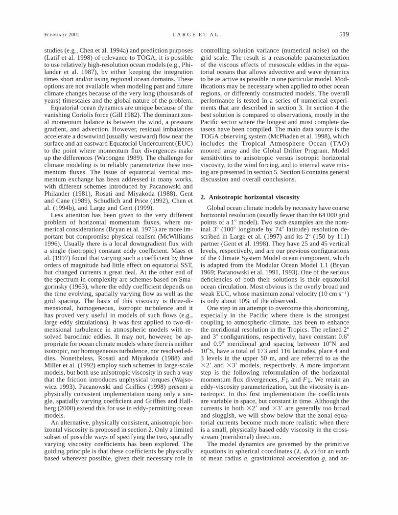
FIG. 2. Zonal sections across the Pacific of zonal velocity at theequator: (a) annual average of case B2, (b) TAO current meter cli-matological annual mean, (c) TAO current meter 1-yr mean, Aug1996–Jul 1997. Contour interval is 10 cm s21 and westward flowregions are shaded.

viscosity equal to the maximum of AMH and BMH, andits near-surface distribution is shown in Fig. 1c. Thisviscosity is governed by large values of BMH only withinabout 208 longitude of tropical and subtropical westernboundaries. Another repeat of B3 (NCEP) used NCEPwind forcing from August 1996 through July 1997, inorder to further quantify the effects of the differentwinds. Finally, the sensitivity to one part of the verticalviscosity (20) was investigated with two repeats of B3;V.5 and V16.7 with set to 0.5 cm2 s21 and to thewnm

16.7 cm2 s21 value of Large et al. (1997), respectively.

4. Comparisons with observations

The better base case result ought to be B2. It haslower mixing coefficients by virtue of its finer resolu-tion, and nonnegative-definite dissipation throughoutthe region of interest (see Fig. 1). Its mean zonal currentsalong the equatorial Pacific (Fig. 2a) are indeed com-parable to the climatological annual mean (Fig. 2b) andthe August 1996 through July 1997 mean (Fig. 2c) fromTAO current meter records. The respective maximumeastward undercurrent velocities, UEUC, are 95.4, 96.4,and 101 cm s21. The improvement over previous modelimplementations with UEUC , 15 cm s21 is dramatic.Also well represented are the rise in the core of the EUCfrom a depth about 200 m in the west to about 70 m inthe east, and the predominantly westward flow near thesurface.

More aspects of the B2 solution will now be comparedto observations in the Pacific and, less extensively, inthe equatorial Atlantic and Indian Oceans. This exerciseleads to the following conclusions regarding differencesfound in these comparisons and in Fig. 2. In the Pacific,the model compares more favorably with spatially av-eraged drifter data than point current meter observations(section 4a). The repeat wind forcing, the monthly pre-cipitation, and the climatological radiation are respon-sible for differences in the monthly mean zonal velocity(section 4b) and hence annual means (Fig. 2). Generalcirculation deficiencies (section 4c) may be causingproblems with modeled currents and water masses northof the equator. With the B2 configuration, specifyingthe horizontal viscosity in the Atlantic remains prob-

lematic (section 4d). Finally, interannual variabilitycould explain differences in the zonal velocity of theIndian Ocean (section 4e).

a. Climatological u(l, f ) and y(l, f ) fromnear-surface drifters

The extensive drifter observations in the equatorialPacific provide the most complete observations of thehorizontal structure of equatorial currents, but horizon-tal averaging over very large bins (28 lat by 128 long)is required because of the sampling. The drogue depthextends between about 10- and 20-m, so the drifter ve-locities are reported at z 5 215 m. The most compatiblemodel velocity is a weighted average of the second lev-el, which spans the depth range 8–17 m and the thirdlevel (17–27 m). Figure 3 shows that the modeled andobserved u(l, f, 215 m) in the Pacific have similar fea-tures. The eastward flowing North Equatorial Counter-current (NECC) is evident between 48 and 88N. Al-though its modeled strength is much stronger than inprevious configurations, it is only about one-half thatobserved across the basin, though the spatial patterns


FIG. 3. Zonal velocity at 15-m depth as a function of latitude andlongitude: (a) annual average of case B2, (b) climatology of equatorialdrifter deployments averaged over 28 lat by 128 long bins. Contourinterval is 10 cm s21, and westward flow regions are shaded.

FIG. 4. As in Fig. 3 except for meridional velocity with a contourinterval of 2 cm s21, and southward flow regions shaded.

are strikingly similar. Both the model and drifters showa maximum in westward flow at about 38S and between1.58 and 3.58N, where it is stronger. In between lies theequator where the model has a sharper feature and moreeastward flow than the drifter data, perhaps due in partto the large meridional averaging of the latter. In themodel this feature is caused by the eastward flowingEUC below.

Analysis of the zonal momentum budget reveals thatthis influence is exerted in two ways. First, there is aturbulent drag characterized by negative momentum flux(s13 , 0) all the way from the EUC core to the surface,such that the term of (1a) and (9) is also negativeuF V

throughout these depths. Thus, this term scales with thezonal surface stress divided by the depth of the EUC.Without an EUC, its magnitude would be greater bymore than a factor of 2, because it would scale with theshallower depth (typically less than 50 m) of the bound-ary layer, where the surface heat and freshwater fluxesare found. Second, there is the upwelling of more east-ward flowing deeper water. In particular, the verticaladvection [wuz part of the (wu)z term of (2)] is not

negligible compared to the zonal pressure gradient inbalancing in (1a). Furthermore, this feature is notuF V

diffused meridionally because remains only aboutuF H

10% of these terms. Without the small value of BMH in(7), away from western boundaries (Fig. 1), this viscousterm would dominate and the role of advection woulddiminish.

Drifter and model meridional velocities at z 5 215m are compared in Fig. 4. They both show similar equa-torial divergence: southward flow at 8–10 cm s21 atabout 28S, and northward flow at 8–10 cm s21 at about38N. Along much of the equator the average meridionalvelocity is near zero in both the model and drifters, butthe latter display more variability. Off the coast of SouthAmerica, the drifters show strong equatorward flow inboth hemispheres, but the model has northward flow inthe Southern Hemisphere only in its 8-m-thick upper-most level.

Prognostic model velocities represent the flow overa three-dimensional model grid cell. Therefore, they arenot directly comparable to current meter observationsfrom a point in space; especially in the highly shearedflows of the equatorial oceans. On the other hand, tra-jectories of surface drifters whose drogues span the


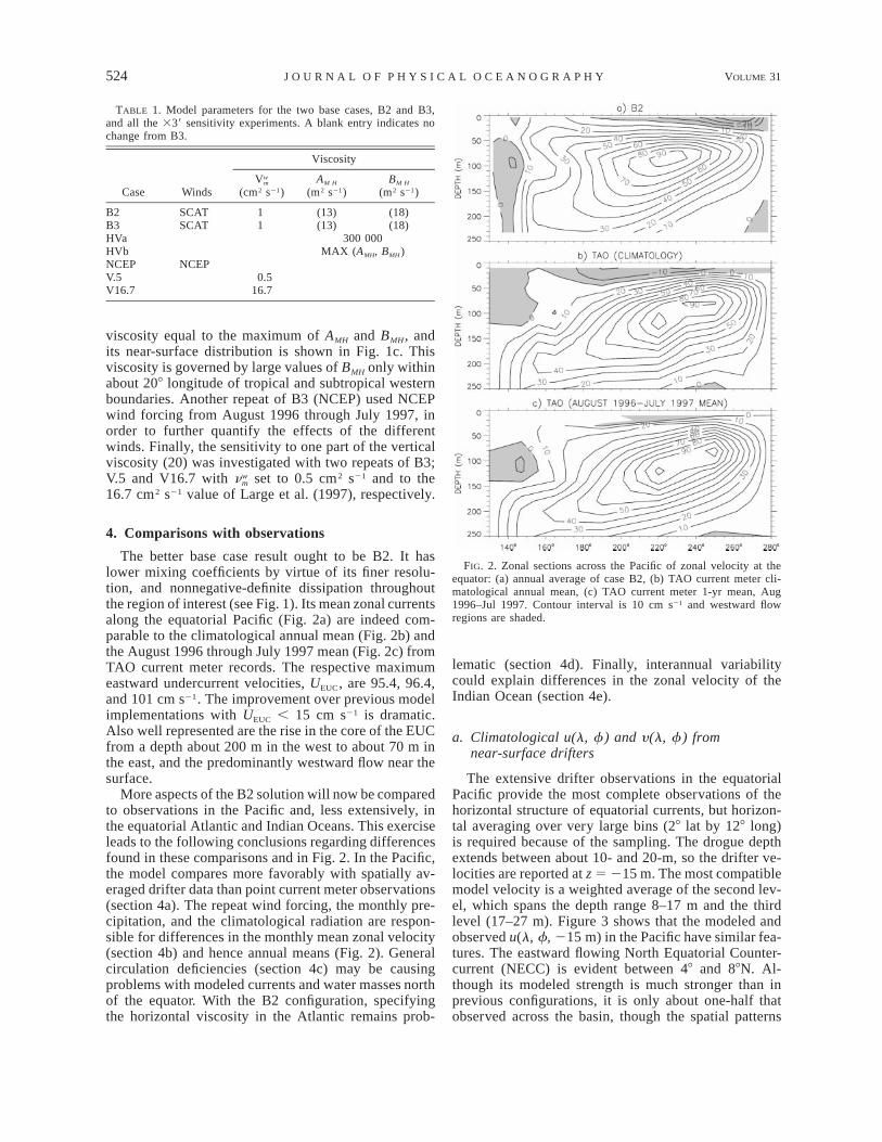
FIG. 5. One year cycle, starting with Aug 1996, of monthly mean zonal velocity at the equator as a functionof depth from case B2 and from the TAO current meters. The two locations are (top) 1478E and (bottom)2208E. The contour interval is 20 cm s21, and westward flow regions are shaded.

depths of a model grid level potentially could providemore compatible velocities. Although the drifter obser-vations fall short of this ideal, we indeed find that insome ways the model (Figs. 2a and 3a) agrees better atthe equator with the spatially averaged drifter data (Fig.3b) than the point current meter climatology (Fig. 2b).For example, the three respective values foru(08, 1608E, 215 m) are about 15, 15, and 0 cm s21 andfor u(08, 2608E, 215 m) they are about 222, 224, and25 cm s21.

b. Annual cycle of zonal velocity profiles

Twelve monthly means (August 1996–July 1997) ofzonal velocity from current meters and the model areshown in Fig. 5. This comparison is complicated by thestrong 1997 ENSO warm event, and this problem mayexplain some of the differences in Fig. 2. The repeatannual cycle of winds is necessary to spin up the modelcurrents and evolve the temperature and salinity awayfrom their initial conditions. There is a smooth transitionof the atmospheric state forcing over the last 5 days ofJuly 1997 and the first 5 days of August 1996, but there

is no attempt to initialize the model with velocity, tem-perature, and salinity fields appropriate for August 1996because the observations are incomplete. Instead, theocean state at the beginning of each August 1996 isrepresentative of July 1997 conditions, and a much poor-er initial condition than would have been the case if1997 had been a more normal year.

Where the observed and modeled currents are similarin August, they tend to remain so throughout the yearand, therefore, the annual means (Fig. 2) compare well.An example is at 2208E, above about 70 m (Fig. 5, lowerpanels). Deeper, such is not the case. In August 1996,the current meters below 150 m show a very stronguniform eastward flow at 100 cm s21 that remains stron-ger than the model throughout the year. As a result, themodel annual mean currents (Fig. 2a) are 10–20 cm s21

smaller at these depths than in Fig. 2c. It would appearthat this problem is also at least partially responsiblefor the shallower and weaker maximum at 2208E in Fig.2a, compared to Fig. 2b and Fig. 2c. However, the ob-served evolution of the EUC at 2208E (its rise fromMarch to June, maximum of more than 140 cm s21 in


April, and disappearance in July) is reproduced by themodel.

The model August conditions are also quite differentthan observed at 1478E (Fig. 5, top panels). Althoughneither the model, nor the current meters display muchmonthly variability below 150 m, the latter display morevertical shear in August and throughout the year. There-fore, the annual means differ, with Fig. 2a displayingmuch less shear between 150 and 200 m depth. Insteadthe corresponding shear appears to develop about 108farther east. Above 150-m depth, the model reproducesmuch of the observed pattern of westward flow. Theinitial westward flow is interrupted by two westerlywind bursts that force eastward flow with peaks in Jan-uary and March. The modeled and observed responsesto the first are similar both in magnitude and depth ofpenetration. However, in March the modeled currents atdepth are stronger eastward, perhaps because the month-ly precipitation, or the climatological radiation allowsthe response to penetrate too deep. Between 1508 and1708E, the model (Fig. 2a) has a maximum u between40 and 70 m depth that is not evident in the climatology(Fig. 2b). Although weaker, such a feature is seen bythe current meters from August 1996 to July 1997 (Fig.2c). This result suggests that the currents west of thedate line and above 100 m are very dependent on theresponse to westerly wind bursts, and that all modelforcing, not just the winds, should resolve the diurnalcycle, and be concurrent with the timeframe of the ob-servations being compared.

c. Meridional sections of climatological temperatureand salinity

Baroclinic pressure gradients are important terms inthe momentum equations (1) and couple the equatorialcurrents to the ocean’s potential temperature, u, and sa-linity, S. Climatological sections of u and S from 108Sto 108N along 1658E, 2058E, and 2508E are shown inJohnson and Moore (1997; Fig. 1). These sections showthat the Levitus and Boyer (1994) and Levitus et al.(1994) climatologies overly smooth the meridionalstructures near the equator. Since these structures arepresent in the model, they are now compared with John-son and Moore (1997). It appears that the model’s gen-eral circulation could be improved to produce more re-alistic water masses north of the equator and at depth.

To illustrate, corresponding sections from case B2 areshown in Fig. 6. South of the equator, the model andobserved water masses are much the same. The salinitymaxima are at the same depth, have similar temperatureand salinity, the same variation with longitude, and pen-etrate to about the same latitude. This penetration isterminated by a salinity front. This front is too strongin the model at 2058E because of a tongue of too freshwater coming from the north between about 80 and 250m. Otherwise the model salinities north of the equatorare comparable to the climatological sections. However,

from 68 to 108N the observed meridional temperaturegradient is systematically stronger than the model,which is related to the model’s weak NECC. The depthof the 208C isotherm is generally in good agreementbetween model and observed sections, but deeper themodel has a warm bias, with some density compensationprovided by overall saltier water.

d. Zonal velocity in the Atlantic Ocean

The anisotropic viscosity formulation of section 2 isless successful in the Atlantic, though a big improve-ment over previous implementations. The annual meanzonal velocity from the modeled Atlantic (Fig. 7a) doesnot compare very well with the current meter recordsof Weisberg and Colin (1986). In these observations thecore of the EUC at 288W varies from about 60 to 100cm s21 eastward, while the Fig. 7a value is less than 35cm s21. By chance, this location is near 258W where(15, 16, 17, and 18) give BMH 5 BMunk 5 Beddy 5 Aeddy

(Fig. 1). It appears as if the rapidly increasing viscosityto the west (upstream) causes the EUC strength to beweak downstream even where the viscosity is morephysical. This is also the case farther east at 48W wherethe current meters report core EUC speeds betweenabout 50 and 80 cm s21, but the model value is still lowat only about 25 cm s21. It is interesting that the depthof the model’s Atlantic EUC does agree with the ob-served behavior. It has a distinct annual cycle at 48Wthat is shallowest in late April at about 65 m, deepeningto 100 m by early October. At 258W the annual cycleis much reduced and the mean depth is only about 60m. Because it is weaker, the EUC does not exert suf-ficient influence near the surface where the flow, there-fore, is more westward than observed at both currentmeter locations. The zonal momentum budget (1a) in-dicates that the role of turbulent drag is similar to thePacific (section 4a), but vertical advection is weaker.

e. Zonal velocity in the Indian Ocean

The annual mean zonal velocity across the modeledequatorial Indian Ocean is shown in Fig. 7b, but theproblem of finding contemporaneous forcing and oceanobservations is particularly acute in this basin. Currentmeter records from the Indian Ocean are dominated bysemiannual period variability in response to the semi-annual fluctuations in the zonal wind stress (Luyten andRoemmich 1982; McPhaden 1982). In accord is Fig. 8,which shows the annual cycle of zonal wind stress andmodel velocity at (0.68S, 728E). The location and ver-tical averaging are chosen to match McPhaden (1982,Fig. 1). Both wind records show zonal stress approach-ing 0.05 N m22 in May and October, with correspondingmaxima in the 0–17-m average current reaching nearly100 cm s21. Westward wind stress tends to occur in twoperiods, January–March and June–August, and in re-sponse the flow reverses; in phase at the surface, and


FIG. 6. Meridional sections from 108S to 108N of potential temperature, u, and salinity, S, from case B2. The locationsnear (top) 1658E, (middle) 2058E, and (bottom) 2508E were chosen to match Johnson and Moore (1997, Fig. 1), as arethe contour intervals of 18C and 0.1 psu.

out-of-phase at depth (Fig. 8c). Such westward stressappears to have been more common in the year August1996 to July 1997 than between January 1973 and May1975 so that the model has stronger near-surface west-ward flow (u , 250 cm s21 for 4 of 12 months, Fig.8b) than the observations (u , 250 cm s21 for 1 of 29

months). This interannual variability is likely a majorsource of the weaker mean eastward flow in the upper200 m of Fig. 7b at 728E than shown in McPhaden(1982, Fig. 3). Deeper, between 160 and 180 m, themodel currents compare most favorably with the lastyear of the observed record, where the monthly mean


FIG. 7. Zonal sections across the Atlantic and Indian Oceans ofannual mean zonal velocity at the equator from case B2. Contourinterval is 10 cm s21 in the Atlantic and 5 cm s21 in the Indian, andwestward flow regions are shaded.

FIG. 8. One year cycle of monthly means from case B2 startingwith Aug 1996 of (a) zonal wind stress, and zonal current averagedover depth (b) 0–17-m, and (c) 147–192-m. The location (728E, 0.68S)and depth intervals were chosen to match McPhaden (1982, Fig. 1)closely.

zonal current varies from 21 to 20 cm s21. The vari-ability of the corresponding model flow in Fig. 8c, likethe near-surface currents (Fig. 8b), is comparable tothese observations, so the viscosity does not appear tobe too large in this region of the Indian Ocean.

5. Model sensitivities

Sensitivity experiments (Table 1) are performed usingthe less computationally demanding 339 configuration.An advantage of the anisotropic viscosity formulationof section 2 is that it explicitly includes how the hori-zontal viscosity should vary with resolution. The sen-sitivities in the 339 should be valid for the 329 becausethe B2 and B3 solutions are very similar with regard toequatorial currents. Thus, the larger area of AMH , BMH

in B3 does not appear to be a serious problem. Themeridional sections along 2208E in Fig. 9 provide anillustration of this similarity, as well as the meridionalstructure of the model solutions. In both, the eastwardflow of the EUC extends from about 15 to 250 m, thecore depth is between 90 and 100 m, with a speed be-tween 90 and 95 cm s21. Also both sections show anasymmetric South Equatorial Current that is stronger

westward to the north and has a minimum right at theequator where the force exerted by the EUC is maximum(section 4a). Except for the weak NECC evident at bothresolutions, the model features are very much like theHawaii to Tahiti shuttle results of Wyrtki and Kilonsky(1984) and the drifter observations (Figs. 3 and 4).

A useful diagnostic of overall model sensitivity, es-pecially with regard to the climatically important SST,is upwelling. Meridional sections from three cases areshown in Fig. 10, where the vertical velocity is an annualmean, averaged between 1808 and 2608E in the Pacific.The expected upwelling on the equator and downwellingpoleward is evident in every case. The strength is about10% stronger in B2 (not shown) than in B3 (Fig. 10a):19.8 versus 17.7 (31026 m s21) for the maximum up-welling and 23.3 versus 22.9 (31026 m s21) for themaximum downwelling. For comparison, the diagnosticmodel of Bryden and Brady (1985) gives a somewhatlarger equatorial upwelling with a maximum of 29 31026 m s21 at about the same depth (50–60 m). Theyalso find a much stronger downwelling below 180 m.Their model uses geostrophy to compute a stronger EUC(UEUC . 120 cm s21), which may cause some of thedifference in vertical velocity.

a. Anisotropic versus isotropic viscosity

Compared to B3, cases HVa and HVb differ only intheir formulation of horizontal viscosity. In HVa it is


FIG. 9. Meridional sections from 108S to 108N of annual meanzonal velocity near 2208E from (a) case B2 and (b) case B3. Contourlevel is 10 cm s21, and westward flow regions are shaded.

FIG. 10. Meridional sections from 108S to 108N of annual meanvertical velocity, averaged from 1808 to 2608E from (a) case B3, (b)case HVa, and (c) case NCEP. The contour interval is 2 3 1026 ms21, and downwelling regions are shaded.

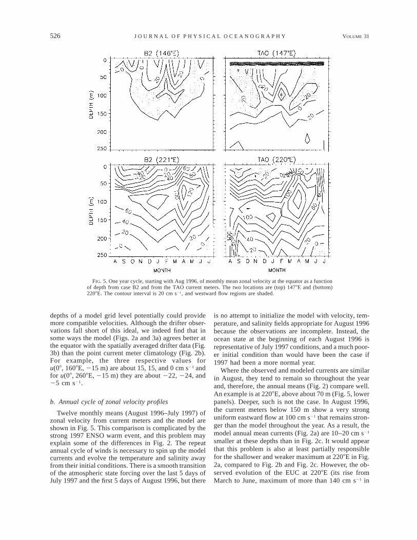
constant and identical to Large et al. (1997) and simi-larly weak equatorial currents result. Compared to B3(Fig. 10a), the much weaker and broader upwelling be-tween 48S and 48N, is shown in Fig. 10b. The upwellingis also shallower, which would tend to bring up warmerwater and maintain a warmer SST. Off the equator thedownwelling in case HVa is as strong, or even strongerthan B3, but shallower and displaced poleward. For themodel resolutions considered here, allowing an isotropicviscosity coefficient to be spatially variable is not veryeffective at strengthening equatorial circulation. To il-lustrate, Fig. 11 shows that the meridional sections ofzonal velocity from HVa and HVb are very similar.There are broad, weak EUCs with deep cores at about130 m. Near the surface both solutions are very differentfrom the drifter observations. The maximum westwardspeeds are right on the equator, not only at 2208E (Fig.11) but across the whole Pacific. Between 58 and 98Nthe NECC is very poorly represented by very weakeastward flows at depth. In contrast to the observations,the near-surface currents are westward at these latitudestoo. Off the equator the poleward velocities are muchtoo weak compared to Fig. 4.

In contrast, anisotropy is very effective in bringingequatorial current speeds and shears up to realistic val-

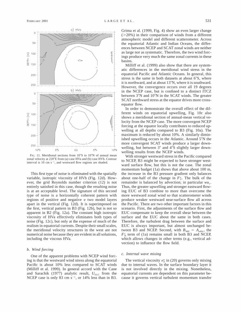
ues. In the Pacific UEUC is increased by nearly an orderof magnitude in B3 (Fig. 9b) compared to HVa and HVb(Fig. 11), and the NECC is much improved. As shownin section 4, other aspects of the equatorial current sys-tems also become more like observations. However, theprice for this improvement is a greater propensity fornumerical noise, as shown by the zonal sections of me-ridional velocity in Fig. 12. Two contour intervals inthese sections are set at 60.05 cm s21; an arbitrary levelof acceptable noise. A design criterion has been to nothave either the plus or minus 0.05 cm s21 contour appearin any noise pattern on the grid scale. Between 400 mand the bottom, where the velocities become small, bothbase cases (Fig. 12a and Fig. 12b) display such noise,but the amplitude criterion is satisfied except for a smallarea at about 400-m depth in both B2 and B3. Verticallycoherent regions of northward flow are separated by2Dl: 4.88 in B2 and 7.28 in B3. This type of noiseappears to emanate from western boundaries and canbe suppressed by reducing the effect of the function,p(x) in (15); the rate at which BMunk decreases away fromwestern boundaries. This can be accomplished by eitherincreasing LM or making N larger in (16), but at the costof reducing the Pacific EUC below its observed strength.


FIG. 11. Meridional sections from 108S to 108N of annual meanzonal velocity at 2208E from (a) case HVa and (b) case HVb. Contourinterval is 10 cm s21, and westward flow regions are shaded.

This first type of noise is eliminated with the spatiallyvariable, isotropic viscosity of HVb (Fig. 12d). How-ever, the grid Reynolds number criterion (12) is notentirely satisfied in this case, though the resulting noiseis at an acceptable level. The signature of this secondtype of noise is a horizontally coherent pattern withregions of positive and negative y two model layersapart in the vertical (Fig. 12d). It is superimposed onthe first, vertical pattern in B3 (Fig. 12b), but is not soapparent in B2 (Fig. 12a). The constant high isotropicviscosity of HVa effectively eliminates both types ofnoise (Fig. 12c), but only at the expense of much of therealism in equatorial currents. Despite their small scales,the meridional velocity structures in the west are notnumerical noise because they are evident in all solutions,including the viscous HVa.

b. Wind forcing

One of the apparent problems with NCEP wind forc-ing is that the westward wind stress along the equatorialPacific is about 10% less compared to SCAT winds(Milliff et al. 1999). In general accord with the Caneand Sarachik (1977) analytic result, UEUC from theNCEP case is only 83 cm s21, or 14% less than in B3.

Grima et al. (1999, Fig. 4) show an even larger change(.20%) in their comparison of winds from a differentatmospheric model and different scatterometer. Acrossthe equatorial Atlantic and Indian Oceans, the differ-ences between NCEP and SCAT zonal winds are neitheras large nor as systematic. Therefore, the two wind forc-ings produce very much the same zonal currents in thesebasins.

Milliff et al. (1999) also show that there are system-atic differences in the meridional wind stress in theequatorial Pacific and Atlantic Oceans. In general, thisstress is the same in both datasets at about 68S, whereit is northward, and at about 138N, where it is southward.However, the convergence occurs over all 19 degreesin the NCEP case, but is confined to a distinct ITCZbetween 38N and 108N in the SCAT winds. The greaterSCAT northward stress at the equator drives more cross-equator flow.

In order to demonstrate the overall effect of the dif-ferent winds on equatorial upwelling, Fig. 10c alsoshows a meridional section of annual-mean vertical ve-locity from the NCEP case. The more convergent NCEPforcing at the equator locally contributes to reduced up-welling at all depths compared to B3 (Fig. 10a). Themaximum is reduced by about 10%. A similarly dimin-ished upwelling occurs in the Atlantic. Around 58N themore convergent SCAT winds produce a larger down-welling, but between 38 and 48S slightly larger down-welling results from the NCEP winds.

With stronger westward stress in the Pacific comparedto NCEP, B3 might be expected to have stronger west-ward surface flow, but this is not the case. The zonalmomentum budget (1a) shows that above about 100 m,the increase in the B3 pressure gradient only balancesabout one-half of the change in . The bulk of theuF V

remainder is balanced by advection; in particular wuz.Thus, the greater upwelling and stronger eastward flow-ing EUC of B3 combine to more than overcome themore westward zonal wind so that scatterometer windsproduce weaker westward near-surface flow all acrossthe Pacific. There are two other important factors in thisscenario. First, the adjustments of the surface flow andEUC compensate to keep the overall shear between thesurface and the EUC about the same in both cases.Therefore, the turbulent drag between the surface andEUC is always important, but almost unchanged be-tween B3 and NCEP. Second, with BMH 5 Aeddy, the

term of (1a) remains small in both B3 and NCEP,uF H

which allows changes in other terms (e.g., vertical ad-vection) to influence the flow field.

c. Internal wave mixing

The vertical viscosity in (20) governs only mixingwnm

due to internal waves. In the surface boundary layer itis not involved directly in the mixing. Nonetheless,equatorial currents are dependent on this parameter be-cause it governs vertical turbulent momentum transfer


FIG. 12. Zonal section of annual mean meridional velocity along the equatorial Pacific from (a) case B2, (b) case B3, (c) case HVa, and(d) case HVb. Contours are irregular at 0, 60.5, 61, 62, 65, 610, 620, 650, 6100, and 6200 mm s21. The zero contour separates shadedsouthward flow from unshaded northward flow.

between the EUC core and deeper waters and it com-bines with shear instability mixing between the core andthe boundary layer. The overall sensitivity of the modelto is found to differ between the Pacific and Atlanticwnm

because horizontal viscosity plays too prominent a rolein the latter. This behavior is shown by comparing thethree cases V.5, B3, and V16.7 (Table 1). The effectson the magnitude (UEUC), depth (DEUC), and longitude(lEUC) of the maximum annual mean zonal velocity ofthe EUC are shown in Table 2. Also shown for bothbasins are the maximum westward surface velocity, Uo,and measures of the overall shear between DEUC and thesurface, SEQ (in units of cm s21 m21) and of the up-welling, WEQ.

With 5 16.7 cm2 s21, the zonal momentum budgetwnm

(1a) in both basins is primarily a simple balance betweenthe pressure gradient and from the surface to belowuF V

DEUC. Below DEUC, where 5 uzz, vertical mixingu wF nV m

with the slow moving abyss is much more of a brakeon the EUC than it should be. This momentum exchangebecomes much less important and perhaps more realistic

in B3 when this viscosity is reduced to 5 1.0 cm2wnm

s21. There is little change in the pressure gradient atany depth, which, with less friction, accelerates theEUC, whose maximum is found at shallower depths andfarther east (Table 2). In V16.7 the low shear, SEQ, meansthat internal wave viscosity dominates mixing betweenthe EUC and boundary layer (20). When this processis reduced in B3, the shear adjusts until shear instabilitymixing can make up the difference, along with increasedadvection. This occurs with SEQ 5 1.3 in both basins(Table 2). The vertical advection increases because ofthe larger shear and the greater upwelling, WEQ. In thePacific, UEUC reaches observed speeds (Fig. 9b) withadvection balancing the pressure gradient at depthsaround DEUC. The larger UEUC provides more thanenough shear, SEQ, and reduces the westward near-sur-face flow, Uo. In the Atlantic the pressure gradient inthe vicinity of DEUC is balanced incorrectly by meridi-onal viscosity, primarily the second term on the right-hand side of (7), because the coefficient, BMH, is un-physically large over too much of this basin. As a result,


TA

BL

E2.

Sen

siti

vity

ofth

ean

nual

mea

neq

uato

rial

zona

lcu

rren

tst

ruct

ure

tove

rtic

alvi

scos

ity

due

toin

tern

alw

aves

,,

inbo

thP

acifi

can

dA

tlan

tic

Oce

ans.

The

max

imum

east

war

dw n m

velo

city

inth

eE

UC

has

asp

eed

UE

UC

and

islo

cate

dat

dept

hD

EU

C,

and

long

itud

el

EU

C.

The

max

imum

upw

elli

ngan

ywhe

real

ong

the

equa

tor

isW

EQ,

and

the

min

imum

surf

ace

velo

city

isU

o.

Am

easu

reof

the

over

all

surf

ace

toE

UC

shea

ris

S EQ

5(U

EU

C2

Uo)

/DE

UC.

Cas

e

w n m(c

m2

s21)

Pac

ific

UE

UC

(cm

s21 )

DE

UC

(m)

lE

UC

(8E

)U

o

(cm

s21)

S EQ

)2

12

1(c

ms

mW

EQ

(mm

s21)

Atl

anti

c

UE

UC

(cm

s21)

DE

UC

(m)

lE

UC

(8E

)U

o

(cm

s21

m2

1)

S EQ

)2

12

1(c

ms

mW

EQ

(mm

s21)

V.5

B3

V16

.7

0.5

1 16.7

100 97 40

95 95 140

232

232

210

234

235

245

1.41

1.39 .61

20 20 12

46 40 11

64 64 105

348

348

338

245

245

234

1.42

1.33 .43

10 10 6

the EUC fails to reach observed speeds (UEUC 5 40 cms21, Table 2) and the westward near-surface flow in-creases until SEQ 5 1.3.

In B3, uzz is not an important term at the depth ofwnm

the EUC. Therefore, the factor of 2 reduction of inwnm

case V.5 causes little change in the EUC of either basin.With a similar EUC, other aspects of the equatorial cur-rents are not very different either (Table 2). This con-vergence of solutions to an equatorial current structureresembling reality means that any value of less thanwnm

about 1.0 cm2 s21 could have been used for the basecases B2 and B3.

6. Discussion and conclusions

A coarse-resolution climate model can be configuredto produce equatorial currents comparable to observa-tions, provided that a certain amount of numerical noiseis accepted. In the present model, the key element isthe spatially variable, anisotropic horizontal viscosity.It allows the coefficient of meridional diffusion of zonalmomentum, BMH, to be a physically based small valueeverywhere except near western boundaries. Thescheme formulated in section 2 includes dependencieson grid size, so parameter values need to be found atonly one resolution. This tuning procedure is greatlysimplified by taking the numerical constraints (11), (12),and (19) to be equalities and by restricting the appli-cation to equatorial oceans, where the EUC requires Vo

5 100 cm s21 in (14). Then, the only open question ishow BMunk (15) should decrease away from westernboundaries. The empirical result, (16) with LM 5 1000km and N 5 3, is a compromise between equatorialcurrent strength and smoothness on the grid scale.

In the central Pacific the 339 horizontal resolution ofDl 5 3.68, Df 5 0.98 (B3) is found to be adequate.The weak, diffuse zonal flows of previous implemen-tations are reproduced in case HVa, with a constant,isotropic viscosity of 300 3 103 m2 s21. There is verylittle improvement with the spatially varying isotropicviscosity of case HVb. On the other hand, the spatiallyvarying anisotropic viscosity of B3 not only improveszonal current structure and strength on and off the equa-tor, it has a profound effect on meridional flow and onequatorial upwelling. Perhaps most significantly, it pro-duces upwelling much deeper where it involves colderwater in the surface heat budget.

Only a combination of BMH 5 Aeddy, scatterometerwind forcing, and less than about 1 cm2 s21 is foundwnm

to produce a central Pacific EUC of the observedstrength. This result may also depend on other aspectsof the vertical viscosity (20). With weaker westwardwind stress, the value of UEUC in a model Pacific drivenby NCEP reanalysis winds is about 10% weaker. It isnot clear what the near-surface current in the modelshould be because neither the point current meter mea-surements nor the drifter bins correspond to the extentof the model grids. Nevertheless, the zonal component


of the model is strongly influenced by turbulent dragand vertical advection from the EUC below. These ef-fects, including weaker upwelling, led to the unexpectedresult that weaker NCEP westward winds produce stron-ger westward near-surface flow in the Pacific. A dif-ferent model momentum balance may not show the sameresponse.

A large value of 5 16.7 cm2 s21 (V16.7) com-wnm

pletely alters the momentum budget at the depths of theEUC because of the excessive downward momentumflux. The divergence of this flux, , deepens and slowsuF V

the EUC and becomes the primary balance of the pres-sure gradient. Once ceases to be important, at 5u wF nV m

1.0 cm2 s21 (B3), there is little sensitivity to furtherreductions of (e.g., V.5). The sensitivity of the near-wnm

surface westward flow to reducing depends on howwnm

the pressure gradient becomes balanced in and belowthe EUC. In the Pacific it is the advection terms, thatallow the EUC to reach observed speeds and reduce thewestward surface flow. In the Atlantic this balancecomes from an excessive meridional viscosity thatmakes the EUC too slow, with the net result that thesurface flow becomes stronger westward. A very dif-ferent sensitivity might be found in the Philander andPacanowski (1984) model because the pressure gradientis not an important term below the thermocline (Wa-congne 1989).

The finest horizontal resolution implemented (329)has Dl 5 2.48, Df 5 0.68 at the equator. Annual meansfrom this case (B2) compare favorably with the exten-sive observations from the equatorial Pacific. Furthercomparison would require a model simulation includingcomprehensive initial conditions, complete and accurateforcing, and contemporaneous observations. In partic-ular, it would be important to avoid problems associatedwith the large interannual variability in this region, suchas the strong 1997 ENSO. Despite this event, the resultsdo suggest that the ocean response to westerly windbursts is an important factor in determining the verticalstructure of annual mean zonal currents in the westerntropical Pacific. The model is capable of a strong re-sponse to such events (e.g., December 1996), but pre-cipitation and radiation forcing, at least daily, may benecessary for the proper modulation (e.g., March 1997).The model’s large-scale general circulation in the Pacificproduces more realistic water masses south of the equa-tor. To the north the water is too fresh and there areweak meridional temperature gradients associated witha weak NECC.

The observational evidence from 728E indicates thatequatorial Indian Ocean currents are not overly atten-uated in B2. The maximum monthly mean EUC speedof nearly 100 cm s21 is comparable to the observations.Annual mean differences with limited current meter re-cords can be attributed to interannual variability, at leastuntil more extensive observations become available.

In the much narrower Atlantic equatorial basin it ap-pears as if the viscosity, BMH, remains too large too far

east of South America, even in the 329. One conse-quence is that the EUC never achieves an eastward ve-locity more than about half of that observed. Some im-provement may be possible by reducing LM and/or N in(16), but the noise penalty would be high for a modestgain. Figure 7 shows the EUC forming at about 358W.If it is assumed that it will be sufficient to have BMH 5Aeddy everywhere downstream of this point, then the re-quired model resolution is about Dl 5 18. Another as-pect that may improve with finer zonal resolution is thedepth of the equatorward surface flow off the coast ofSouth America.

We view the formulation presented in section 2 forspatially variable, anisotropic eddy viscosities as pro-visional, so we have not been concerned with havingAMH , BMH away from our present regions of focus.With it we have achieved more satisfactorily strong andnarrow equatorial currents in a coarse-resolution oceanmodel than with simpler formulations. Only at very fineresolution (Dl 5 Df 5 0.18) does the viscosity becomenearly isotropic with a coefficient close to Aeddy, subjectto (19). Such resolutions have only been configured forregional domains (e.g., Smith et al. 2000) and are notpractical for global climate applications. Anisotropichorizontal eddy viscosity is a practical alternative, al-though Dl 5 2.48 would appear to be too coarse in theAtlantic. We believe there may be further benefits withadaptive prescriptions for the coefficients, that is, func-tionals of the solution fields as well as the grid structure.

Acknowledgments. We wish to acknowledge the manyindividuals responsible for acquiring the equatorialocean observations used in this study. In particular, theTOGA TAO Project Office, Dr. M. J. McPhaden, Di-rector, made the TOGA TAO data freely and easily ac-cessible, and Dr. P. P. Niiler generously provided pro-cessed surface drifter velocities. Dr. Rick Smith pro-vided helpful insights into general viscosity formula-tions. The National Center for Atmospheric Research issponsored by the National Science Foundation.

REFERENCES

Batchelor, G. K., 1967: An Introduction to Fluid Dynamics. Cam-bridge University Press, 615 pp.

Biasutti, M., and D. S. Battisti, 2001: Low-frequency variability inthe tropical Atlantic as simulated by the NCAR climate systemmodel and the CCM3 coupled to a slab ocean model. J. Climate,submitted.

Bishop, J. K. B., and W. B. Rossow, 1991: Spatial and temporalvariability of global surface solar irradiance. J. Geophys. Res.,96, 16 839–16 858.

Bryan, K., 1969: A numerical method for the study of the circulationof the World Ocean. J. Comput. Phys., 4, 347–376., S. Manabe, and R. C. Pacanowski, 1975: A global ocean–atmosphere climate model. Part II: The oceanic circulation. J.Phys. Oceanogr., 5, 30–46.

Bryden, H. L., and E. C. Brady, 1985: Diagnostic model of the three-dimensional circulation in the upper equatorial Pacific Ocean. J.Phys. Oceanogr., 15, 1255–1273.

Cane, M. A., and E. S. Sarachik, 1977: Forced baroclinic ocean


motions. Part II: The linear equatorial bounded case. J. Mar.Res., 37, 355–398.

Carton, J. A., X. Cao, B. S. Giese, and A. M. daSilva, 1996: Decadaland interannual SST variability in the tropical Atlantic Ocean.J. Phys. Oceanogr., 26, 1165–1175.

Chen, D., A. J. Busalacchi, and L. M. Rothstein, 1994a: The rolesof vertical mixing, solar radiation, and wind stress in a modelsimulation of the sea surface temperature seasonal cycle inthe tropical Pacific Ocean. J. Geophys. Res., 99, 20 345–20 359., L. M. Rothstein, and A. J. Busalacchi, 1994b: A hybrid verticalmixing scheme and its applications to tropical ocean models. J.Phys. Oceanogr., 24, 2156–2179.

Delecluse, P., M. K. Davey, Y. Kitamura, S. G. H. Philander, M.Suarez, and L. Bengtsson, 1998: Coupled general circulationmodeling of the tropical Pacific. J. Geophys. Res., 103, 14 357–14 374.

Freeland, H. J., P. B. Rhines, and H. T. Rossby, 1975: Statisticalobservations of the trajectories of neutrally buoyant floats in theNorth Atlantic. J. Mar. Res., 33, 383–404.

Gent, P. R., and M. A. Cane, 1989: A reduced gravity, primitiveequation model of the upper equatorial ocean. J. Comput. Phys.,81, 444–480., F. O. Bryan, G. Danabasoglu, S. C. Doney, W. R. Holland, W.G. Large, and J. C. McWilliams, 1998: The NCAR ClimateSystem Model Global Ocean Component. J. Climate, 11, 1287–1306.

Gill, A. E., 1982: Atmosphere–Ocean Dynamics. Academic Press,662 pp.

Griffies, S. M., and R. W. Hallberg, 2000: Biharmonic friction witha Smagorinsky-like viscosity for use in large-scale eddy-per-mitting ocean models. Mon. Wea. Rev., 128, 2935–2946.

Grima, N., A. Bentamy, K. Katsaros, Y. Quilfen, P. Delecluse, andC. Levy, 1999: Sensitivity of an oceanic general circulation mod-el forced by satellite wind stress fields. J. Geophys. Res., 104,7967–7989.

Hastenrath, S., 1991: Climate Dynamics of the Tropics. Kluwer Ac-ademic, 488 pp.

Johnson, G. C., and D. W. Moore, 1997: The Pacific subsurface coun-tercurrents and an inertial model. J. Phys. Oceanogr., 27, 2448–2459.

Kalnay, E., and Coauthors, 1996: The NCEP/NCAR 40-Year Re-analysis Project. Bull. Amer. Meteor. Soc., 77, 437–471.

Large, W. G., and P. R. Gent, 1999: Validation of vertical mixing inan equatorial ocean model using large eddy simulations andobservations. J. Phys. Oceanogr., 29, 449–464., J. C. Williams, and S. C. Doney, 1994: Oceanic vertical mixing:A review and a model with a nonlocal boundary layer param-eterization. Rev. Geophys., 32, 363–403., G. Danabasoglu, S. C. Doney, and J. C. McWilliams, 1997:Sensitivity to surface forcing and boundary layer mixing in aglobal ocean model: Annual mean climatology. J. Phys. Ocean-ogr., 27, 2418–2447.

Latif, M., D. Anderson, T. Barnett, M. Cane, R. Kleeman, A. Leetmaa,J. J. O’Brien, A. Rosati, and E. Schneider, 1998: A review ofthe predictability and prediction of ENSO. J. Geophys. Res., 103,14 375–14 394.

Levitus, S., and T. P. Boyer, 1994: World Ocean Atlas 1994. Vol. 4:Temperature. NOAA Atlas NESDIS 4, U.S. Department of Com-merce, Washington, D.C., 117 pp., R. Burgett, and T. P. Boyer, 1994: Salinity. Vol. 3, World OceanAtlas 1994. National Oceanic and Atmospheric Administration,99 pp.

Love, A. E. H., 1944: A Treatise on the Mathematical Theory ofElasticity. Dover, 643 pp.

Luyten, J. R., and D. H. Roemmich, 1982: Equatorial currents atsemi-annual period in the Indian Ocean. J. Phys. Oceanogr., 12,406–413.

Maes, C., G. Madec, and P. Delecluse, 1997: Sensitivity of an equa-

torial Pacific OGCM to the lateral diffusion. Mon. Wea. Rev.,125, 958–971.

McPhaden, M. J., 1982: Variability of the central equatorial IndianOcean. Part I: Ocean dynamics. J. Mar. Res., 40, 157–176., and Coauthors, 1998: The Tropical Ocean–Global Atmosphereobserving system. J. Geophys. Res., 103, 14 169–14 240.

McWilliams, J. C., 1996: Modeling the oceanic general circulation.Annu. Rev. Fluid Mech., 23, 215–248., and J. H. S. Chow, 1981: Equilibrium geostrophic turbulence.Part I: A reference solution in a b-plane channel. J. Phys. Ocean-ogr., 11, 921–949., and Coauthors, 1983: The local dynamics of eddies in thewestern North Atlantic. Eddies in Marine Science, A. R. Rob-inson, Ed., Springer-Verlag, 92–113.

Miles, J., 1994: On transversely isotropic eddy viscosity. J. Phys.Oceanogr., 24, 1077–1079.

Miller A. J., J. M. Oberhuber, N. E. Graham, and T. M. Barnett, 1992:Tropical Pacific Ocean response to observed winds in a layeredgeneral circulation model. J. Geophys. Res., 97, 7317–7340.

Milliff, R. F., W. G. Large, J. Morzel, G. Danabasoglu, and T. M.Chin, 1999: Ocean general circulation model sensitivity to forc-ing from scatterometer winds. J. Geophys. Res., 104, 11 337–11 358.

Munk, W. H., 1950: On the wind driven ocean circulation. J. Meteor.,7, 79–93.

Pacanowski, R. C., and S. G. H. Philander, 1981: Parameterizationof vertical mixing in numerical models of the tropical oceans.J. Phys. Oceanogr., 11, 1443–1451., and S. M. Griffies, 1998: MOM 3.0 manual. NOAA/GFDL,668 pp. [Available from NOAA/Geophysical Fluid DynamicsLaboratory, Princeton, NJ 08542.], K. Dixon, and A. Rosati, 1991, 1993: The GFDL modular oceanmodel users guide. GFDL Ocean Group Tech. Rep. 2. [Availablefrom NOAA/GFDL, Princeton, NJ 08542.]

Philander, S. G. H., 1990: El Nino, La Nina, and the Southern Os-cillation. Academic Press, 289 pp., and R. C. Pacanowski, 1984: Simulation of the seasonal cyclein the tropical Atlantic Ocean. Geophys. Res. Lett., 11, 802–804., W. J. Hurlin, and A. D. Siegel, 1987: Simulation of the seasonalcycle of the tropical Pacific Ocean. J. Phys. Oceanogr., 17,1986–2002.

Rosati, A., and K. Miyakoda, 1988: A general circulation model forupper ocean simulation. J. Phys. Oceanogr., 18, 1601–1626,

Rossow, W. B., and R. A. Schiffer, 1991: ISCCP cloud data products.Bull. Amer. Meteor. Soc., 72, 2–20.

Schudlich, R. R., and J. F. Price, 1992: Diurnal cycles of current,temperature, and turbulent dissipation in a model of the equa-torial upper ocean. J. Geophys. Res., 97, 5409–5422.

Smagorinsky, J., 1963: General circulation experiments with theprimitive equations. Mon. Wea. Rev., 91, 99–164.

Smith, R. D., M. E. Maltrud, F. O. Bryan, and M. W. Hecht, 2000:Numerical simulation of the North Atlantic Ocean at 1⁄108. J. Phys.Oceanogr., 30, 1532–1561.

Stockdale, T. N., A. J. Busalacchi, D. E. Harrison, and R. Seager,1998: Ocean modeling for ENSO. J. Geophys. Res., 103, 14 325–14 356.

Wacongne, S., 1989: Dynamical regimes of a fully nonlinear stratifiedmodel of the Atlantic Equatorial Undercurrent. J. Geophys. Res.,94, 4801–4815.

Wajsowicz, R. C., 1993: A consistent formulation of the anisotropicstress tensor for use in models of the large-scale ocean circu-lation. J. Comput. Phys. 105, 333–338.

Weaver, A. J., and E. S. Sarachik, 1991: Reply. J. Phys. Oceanogr.,21, 1702–1707.

Webster, P. J., V. O. Magana, T. N. Palmer, J. Shukla, R. A. Tomas,M. Yani, and T. Yasunari, 1998: Monsoons: Processes, predict-ability, and the prospects for prediction. J. Geophys. Res., 103,14 451–14 510.

Weisberg, R. H., and C. Colin, 1986: Equatorial Atlantic Ocean tem-


perature and current variations during 1983 and 1984. Nature,322, 240–243.

Williams, G. P., 1972: Friction term formulation and convective in-stability in a shallow atmosphere. J. Atmos. Sci., 29, 870–876.

Wyrtki, K., and B. Kilonsky, 1984: Mean water and current structure

during the Hawaii to Tahiti shuttle experiment. J. Phys. Ocean-ogr., 14, 242–254.

Xie, P., and P. A. Arkin, 1996: Analyses of global monthly precipi-tation using gauge observations, satellite estimates, and numer-ical model predictions. J. Climate, 9, 840–858.

equatorial circulation of a global ocean climate model

Documents