Seminar on

Thermodynamic analysis of ocean circulation

Master of Technology

In

Earth Systems & Sciences,

Center for Ocean,Rivers,Atmosphere and Land Sciences,

Indian Institute of Technology, Kharagpur

Presented by: Himanshu Katiyar (14CL60R03)

1

SUMMARY

• Calculating a stream function as function of depth and density isproposed as a new way of analyzing the thermodynamic characterof the overturning circulation in the global ocean.

• The sign of an overturning cell in this stream function directly showswhether it is driven mechanically by large-scale wind stress orthermally by heat conduction and small-scale mixing.

• It is also shown that the integral of this stream function gives thethermodynamic work performed by the fluid. The analysis is alsovalid for the Boussinesq equations, although formally there is nothermodynamic work in an incompressible fluid.

INTRODUCTION• A common way of analyzing the energetics of the ocean

circulation is to perform bulk calculations and construct boxdiagrams.

• Such a diagram can be regarded as a zero-dimensional picture ofthe ocean, with no spatial degrees of freedom.

• A principal problem with these models is that the particletrajectories in a three-dimensional fluid are in general not closed.

• Thus, the stream function in depth–density coordinates gives atwo-dimensional thermodynamic picture of the oceancirculation, without any assumption about closed particletrajectories.

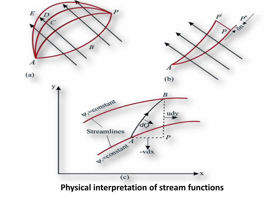
Physical interpretation of stream functions

Objectives

• Calculation of work done by thermal forces

• Analysis of energetics of the Boussinesqequations (Illustration of the budget equationsfor the Kinetic energy K and the Potential energyU in a Boussinesq model)

Work done by thermal forces

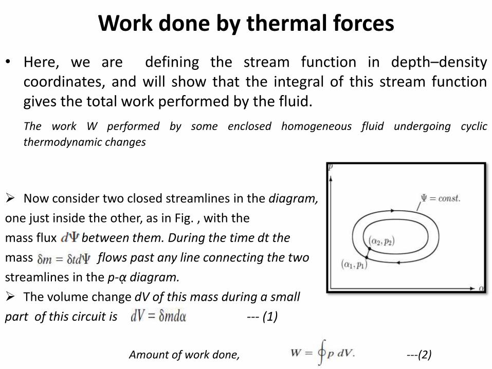
• Here, we are defining the stream function in depth–densitycoordinates, and will show that the integral of this stream functiongives the total work performed by the fluid.

The work W performed by some enclosed homogeneous fluid undergoing cyclic

thermodynamic changes

Now consider two closed streamlines in the diagram,

one just inside the other, as in Fig. , with the

mass flux between them. During the time dt the

mass flows past any line connecting the two

streamlines in the p-ᾳ diagram.

The volume change dV of this mass during a small

part of this circuit is --- (1)

Amount of work done, ---(2)

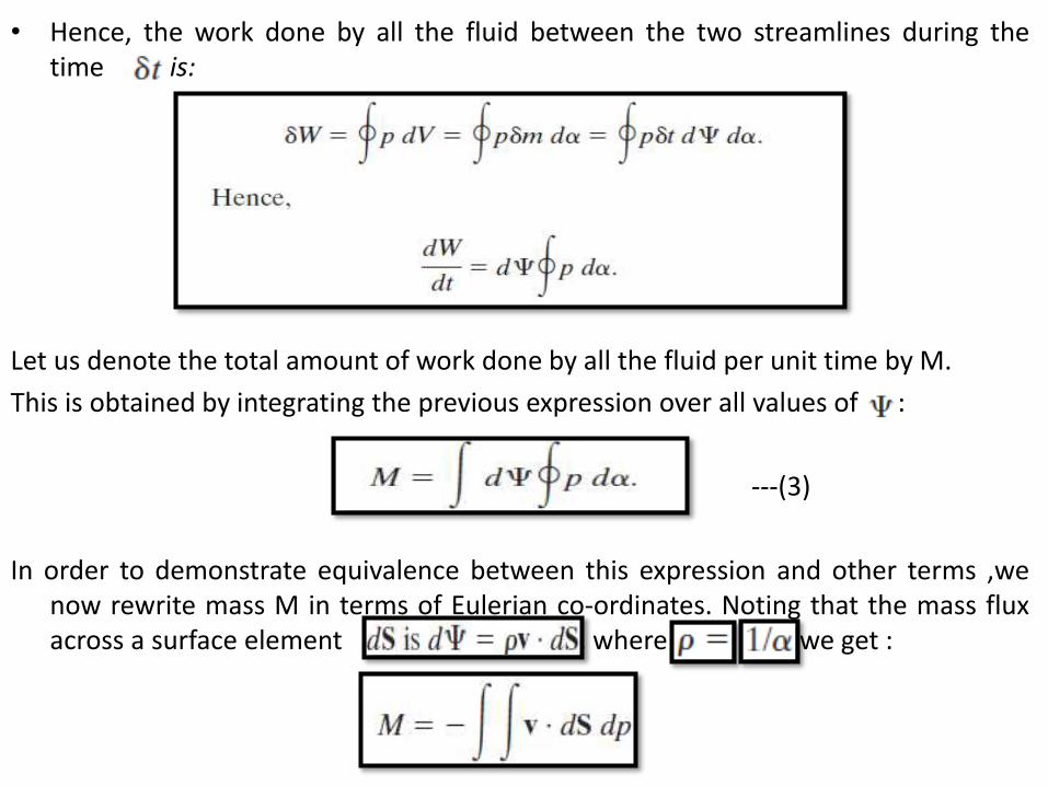
• Hence, the work done by all the fluid between the two streamlines during thetime is:

Let us denote the total amount of work done by all the fluid per unit time by M.

This is obtained by integrating the previous expression over all values of :

---(3)

In order to demonstrate equivalence between this expression and other terms ,wenow rewrite mass M in terms of Eulerian co-ordinates. Noting that the mass fluxacross a surface element , where , we get :

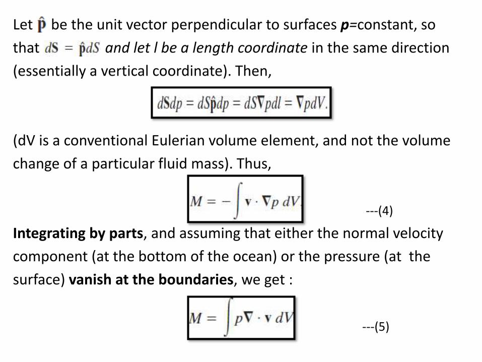
Let be the unit vector perpendicular to surfaces p=constant, so

that , and let l be a length coordinate in the same direction

(essentially a vertical coordinate). Then,

(dV is a conventional Eulerian volume element, and not the volume

change of a particular fluid mass). Thus,

---(4)

Integrating by parts, and assuming that either the normal velocity

component (at the bottom of the ocean) or the pressure (at the

surface) vanish at the boundaries, we get :

---(5)

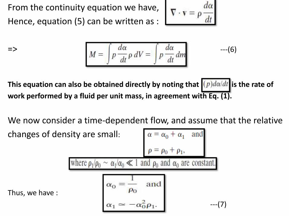
From the continuity equation we have,

Hence, equation (5) can be written as :

=> ---(6)

This equation can also be obtained directly by noting that is the rate of

work performed by a fluid per unit mass, in agreement with Eq. (1).

We now consider a time-dependent flow, and assume that the relative

changes of density are small:

Thus, we have :

---(7)

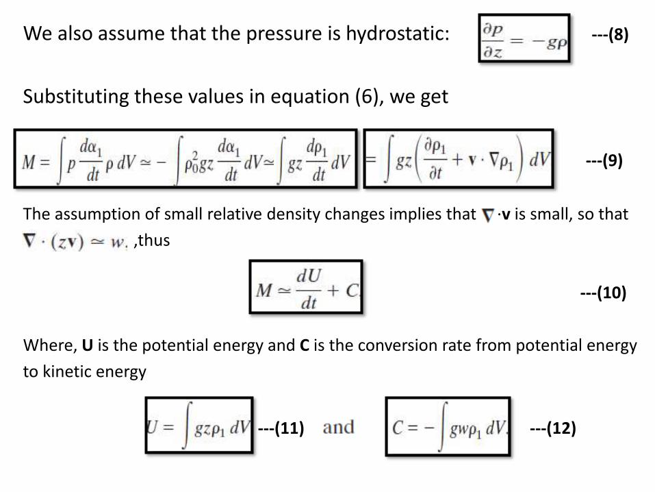
We also assume that the pressure is hydrostatic: ---(8)

Substituting these values in equation (6), we get

---(9)

The assumption of small relative density changes implies that ·v is small, so that

,thus

---(10)

Where, U is the potential energy and C is the conversion rate from potential energy

to kinetic energy

---(11) ---(12)

Thus, if the circulation is stationary (i.e dU/dt=0), and relative density variation is small, the total thermodynamic work done by the fluid is the same as the conversion from potential to kinetic energy.

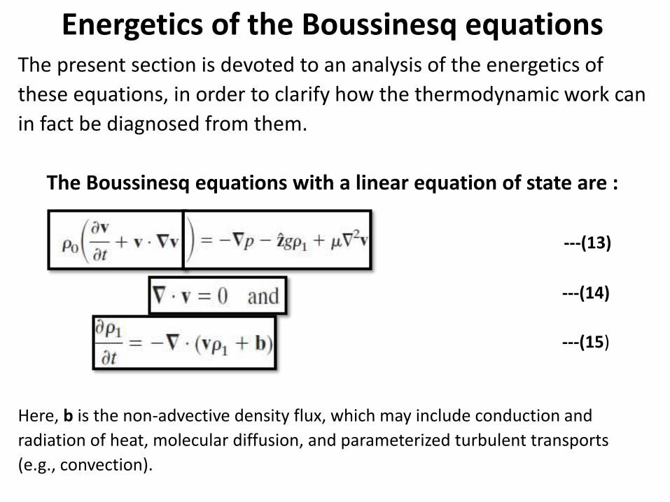
Energetics of the Boussinesq equationsThe present section is devoted to an analysis of the energetics of

these equations, in order to clarify how the thermodynamic work can

in fact be diagnosed from them.

The Boussinesq equations with a linear equation of state are :

---(13)

---(14)

---(15)

Here, b is the non-advective density flux, which may include conduction and

radiation of heat, molecular diffusion, and parameterized turbulent transports

(e.g., convection).

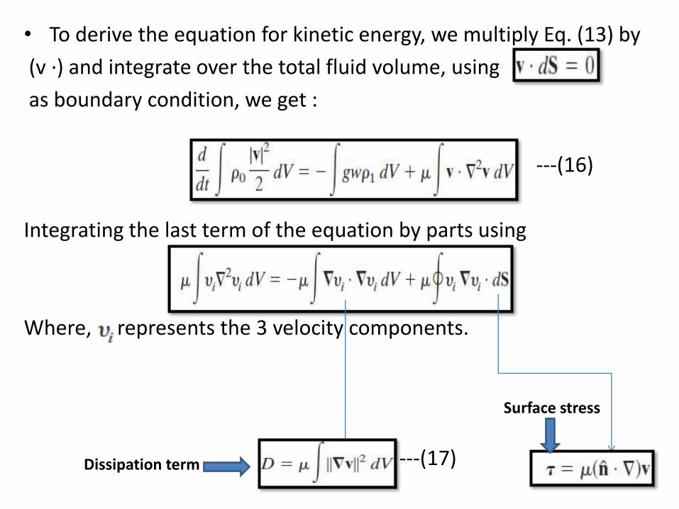
• To derive the equation for kinetic energy, we multiply Eq. (13) by

(v ·) and integrate over the total fluid volume, using

as boundary condition, we get :

---(16)

Integrating the last term of the equation by parts using

Where, represents the 3 velocity components.

---(17)Dissipation term

Surface stress

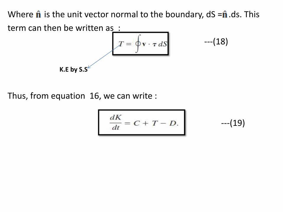
Where is the unit vector normal to the boundary, dS = .ds. This

term can then be written as :

---(18)

Thus, from equation 16, we can write :

---(19)

K.E by S.S

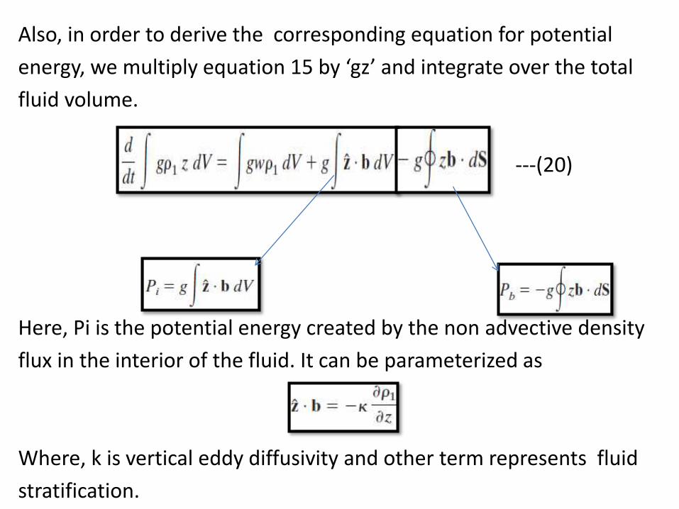
Also, in order to derive the corresponding equation for potential

energy, we multiply equation 15 by ‘gz’ and integrate over the total

fluid volume.

---(20)

Here, Pi is the potential energy created by the non advective density

flux in the interior of the fluid. It can be parameterized as

Where, k is vertical eddy diffusivity and other term represents fluid

stratification.

• The quantity is the potential energy created by density fluxes across the boundaries. At points where b.dS <0, there is increase in P.E.

From equation 20, we can depict that :

---(21)

Thus, from equation 19 and 21,

---(22)

Rate of change of total energy

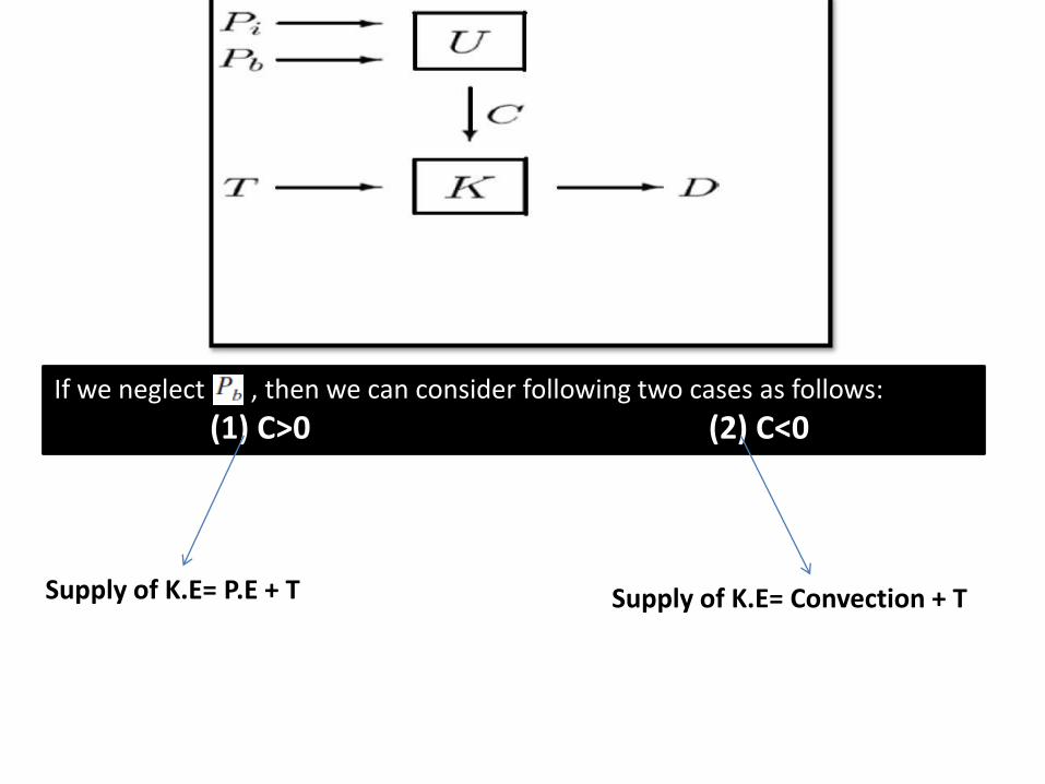
If we neglect , then we can consider following two cases as follows:

(1) C>0 (2) C<0

Supply of K.E= P.E + T Supply of K.E= Convection + T

Considering the work performed by thermal forces, if we compare

equation 10 and equation 21, we get

• If we wish to calculate thermodynamic work in simulation of Boussinesq equations, above equation can be used.

• In case, circulation is stationary (i.e., dU/dt =0), then from eq. 10 and 12,

From (for mass flux), we can define , where, is the

volume flux ( ). Thus,

No pressure term --- (23)

CONCLUSION

• Although the pressure forces strictly speaking performno work in a Boussinesq fluid, the thermodynamic workinstead appears as the generation of potential energy byheat conduction.

• The thermodynamic work can be calculated as anintegral of the stream function in a z- diagram.

REFERENCES• Gade, H. G., and K. E. Gustafsson, 2004: Application of classical

thermodynamic principles to the study of oceanic overturning circulation. Tellus, 56A, 371–386.

• Huang, R. X., 1999: Mixing and energetics of the oceanic thermohaline circulation. J. Phys. Oceanography, 29, 727–746.

• Wunsch, C., and R. Ferrari, 2004: Vertical mixing, energy, and the general circulation of the oceans. Annu. Rev. Fluid Mech., 36, 281–314.

• Jeffreys, H. W., 1925: On fluid motions produced by differences of temperature and salinity. Quart. J. Roy. Meteor. Soc., 51, 347–356.

• Defant, A., 1961: Physical Oceanography. 1, Pergamon Press, 729 pp.

THANK YOU!