efﬁcient optimal control of smoke using spacetime multigrid · efﬁcient optimal control of...

Efficient Optimal Control of Smoke using Spacetime MultigridZherong Pan Dinesh Manocha 1

Department of Computer Sciencethe University of North Carolina

We present a novel algorithm to control the physically-based animation ofsmoke. Given a set of keyframe smoke shapes, we compute a dense se-quence of control force fields that can drive the smoke shape to match sev-eral keyframes at certain time instances. Our approach formulates this con-trol problem as a PDE constrained spacetime optimization and computeslocally optimal control forces as the stationary point of the Karush-Kuhn-Tucker conditions. In order to reduce the high complexity of multiple passesof fluid resimulation, we utilize the coherence between consecutive fluidsimulation passes and update our solution using a novel spacetime full ap-proximation scheme (STFAS). We demonstrate the benefits of our approachby computing accurate solutions on 2D and 3D benchmarks. In practice, weobserve more than an order of magnitude improvement over prior methods.

Additional Key Words and Phrases: Fluid Simulation, Optimal Control

1. INTRODUCTION

Physically-based fluid animations are widely used in computergraphics and related areas. Over the past few years, research influid simulation has advanced considerably and it is now possibleto generate plausible animations for movies and special effects in afew hours on current desktop systems. In this paper, we mainlydeal with the problem of the keyframe-based spacetime controlof smoke, a special kind of fluid. Given a set of keyframe smokeshapes, our goal is to compute a dense sequence of control forcessuch that the smoke can be driven to match these keyframes at cer-tain time instances. This problem is an example of directable an-imation and arises in different applications, including special ef-fects [Rasmussen et al. 2004] (to model a character made of liquid)or artistic animation [Angelidis et al. 2006] (to change the movingdirection of the smoke plume). Some of these control techniques,such as [Nielsen and Bridson 2011], are used in the commercialfluid software.

In practice, the keyframe-based control of fluids is still regardedas a challenging problem. Unlike fluid simulation, which deals withthe problem of advancing the current fluid state to the next oneby time integrating the Navier-Stokes equations, a fluid controllerneeds to consider an entire sequence of fluid states that results in ahigh dimensional space of possible control forces. For example, tocontrol a 3D smoke animation discretized on a uniform grid at res-olution 643 with 60 timesteps, the dimension of the resulting spaceof control forces can be as high as 108. The problem of comput-ing the appropriate control force sequence in such a high dimen-sional space can be challenging for any continuous optimizationalgorithm. Furthermore, the iterative computation of control forceswould need many iterations, each of which involves solving a 2Dor 3D fluid simulation problem that can take hours on a desktopsystem.

Fluid control problems have been well studied in computergraphics and animation. At a broad level, prior techniques can beclassified into proportional-derivative (PD) controllers and optimalcontrollers. PD controllers [Fattal and Lischinski 2004; Shi and Yu2005] guide the fluid body using additional ghost force terms that

SpacetimeOptimization

Keyframe

Initial Frame

Control Force Fields

Fig. 1: Given the keyframe, we use spacetime optimization to compute adense sequence of control force fields, matching a smoke ball to the letter“F” (in the leftmost column). We highlight the control force fields. Five suchanimations are generated, matching the smoke ball to the word “FLUID”,at resolution 1282 with 40 timesteps. Each of these optimization computa-tions take about half an hour on a desktop PC, and is about 17 times fasterthan conventional gradient-based optimizer.

are designed based on a distance measure between the current fluidshape and the keyframe. On the other hand, optimal controllers[Treuille et al. 2003; McNamara et al. 2004] formulate the prob-lem as a spacetime optimization over the space of possible con-trol forces constrained by the fluid governing equations, i.e., theNavier-Stokes equations. The objective function of this optimiza-tion formulation consists of two terms: The first term requires thefluid shape to match the keyframe shape at certain time instances,while the second term requires the control force magnitudes to beas small as possible. Optimal controllers are advantageous over PDcontrollers in that they search for the control forces with the small-est possible magnitude, which usually provide smoother keyframetransitions as well as satisfy the fluid dynamic constraints. Treuilleet al. [2003] and McNamara et al. [2004] use a simple gradient-based optimization to search for control forces. Although thesetechniques reduce the overhead by constraining the control forcesto a small set of force templates, each gradient evaluation still needsto solve a fluid simulation problem, which can slow down the over-all computation.

We present a new, efficient optimization algorithm for control-ling smoke. Our approach exploits the special structure of theNavier-Stokes equations discretized on a regular staggered grid.The key idea is to solve the optimization problem by findingthe stationary point of the first order optimality (Karush-Kuhn-Tucker) conditions [Nocedal and Wright 2006]. Unlike prior meth-ods [Treuille et al. 2003; McNamara et al. 2004] that only solvefor the primal variables, we maintain both the primal and dual vari-ables (i.e., the Lagrangian multipliers). By maintaining the addi-tional dual variables, we can iteratively update our solution withoutrequiring it to satisfy the Navier-Stokes equations exactly in eachiteration, thus avoiding repeated fluid simulation. In order to updatethe solution efficiently, we present a spacetime full approximation

ACM Transactions on Graphics, Vol. VV, No. N, Article XXX, Publication date: Month YYYY.

arX

iv:1

608.

0110

2v1

[cs

.GR

] 3

Aug

201

6

2 ●

scheme (STFAS), which is a spacetime nonlinear multigrid solver.Our multigrid solver uses a novel spacetime smoothing operatorand can converge within a number of iterations independent of thegrid resolution and the number of timesteps. Overall, some novelaspects of our approach include:

—A spacetime optimization solver for controlling smoke anima-tion. We formulate it using a fixed point iteration defined for theKKT conditions.

—An acceleration scheme for the fixed point iteration using aspacetime full approximation scheme (STFAS).

—A keyframe-based smoke control algorithm that can efficientlyfind high resolution control forces to direct long 2D and 3D fluidanimation sequences. Moreover, a user can easily balance thekeyframe matching exactness and the amount of smoke-like be-havior by tuning a control force regularization parameter.

We have evaluated our approach on several benchmarks. Ourbenchmarks vary in terms of the grid resolution, the number oftimesteps, and the control force regularization parameter. We high-light results with up to 60 timesteps at the resolution of 643. More-over, we allow each component of the velocity field to be con-trolled. In practice, our algorithm can compute a convergent anima-tion in less than 50 iterations, and the overall runtime performanceis about an order of magnitude faster than a gradient-based quasi-Newton optimizer [Nocedal and Wright 2006] for similar accuracy.An example of achieved smooth transitions between keyframes isillustrated in Figure 1.

2. RELATED WORK

In this section, we give a brief overview of prior techniques for fluidsimulation, multigrid solvers and animation control algorithms.

Fluid simulation has been an active area of research in bothcomputer graphics and computational fluid dynamics. The simula-tion of fluid is typically solved by a discretized time integration ofthe Navier-Stokes equations or their equivalent forms. At a broadlevel, prior fluid simulators can be classified into Lagrangian orEulerian solvers according to the discretization of the convectionoperator. In order to model smoke and fire, a purely Eulerian solver[Fedkiw et al. 2001] is the standard technique. In terms of free-surface flow, hybrid Lagrangian-Eulerian representation [Zhu andBridson 2005] has been widely used in computer graphics. In ourwork, we confine ourselves to the control of fluids without free-surface, i.e., smoke or fire. We use [Harlow and Welch 1965] asour underlying fluid simulator.

Multigrid solvers are widely used for fluid simulation. Multi-grid is a long-standing concept that has been widely used to effi-ciently solve linear systems discretized from elliptic partial differ-ential equations (see [Trottenberg and Schuller 2001]). This ideahas been successfully applied to fluid simulation [Chentanez et al.2007; Chentanez and Muller 2011; Zhang and Bridson 2014] tofind the solenoidal component of the velocity field. In terms ofPDE-constrained optimization and control theory, the idea of multi-grid acceleration has been extended to the spatial temporal domain.Borzi and Griesse [2005] proposed a semi-coarsening spacetimemultigrid to control the time-dependent reaction-diffusion equa-tion. Hinze et al. [2012] used a spacetime multigrid to solve the ve-locity tracking problem governed by the Navier-Stokes equations.

Fluid control problems tend to be challenging and computation-ally demanding. Compared to other kinds of animations, e.g., char-acter locomotion [Mordatch et al. 2012], the configuration space offluid body is of much higher dimension. Prior work in this area can

be classified into two categories: PD controllers [Fattal and Lischin-ski 2004; Shi and Yu 2005] and optimal controllers [Treuille et al.2003; McNamara et al. 2004]. PD controllers compute the controlforces by considering only the configuration of the fluid at the cur-rent and next time instance. For example, in [Shi and Yu 2005], aPD controller is used where the control forces are made propor-tional to the error between the current fluid shape and the targetkeyframe shape. Similar ideas are used for controlling smoke [Fat-tal and Lischinski 2004] and liquid [Shi and Yu 2005; Raveendranet al. 2012]. In contrast, optimal controllers search for a sequenceof control forces that minimize an objective function. Prior meth-ods [Treuille et al. 2003; McNamara et al. 2004] typically solvespacetime optimization over a high-DOF search space to computesuch control forces. Recently, these two methods have been com-bined [Pan et al. 2013] by first optimizing for the fluid shape ateach keyframe and then propagating the changes to the neighbor-ing timesteps. Fluid control can also be achieved by combining ormodifying the results of existing fluid simulation data [Raveendranet al. 2014] or guiding fluid using a designed low-resolution ani-mation [Nielsen and Bridson 2011; Nielsen and Christensen 2010].Our approach is also based on the spacetime optimization formula-tion, similar to [Treuille et al. 2003; McNamara et al. 2004].

In addition, there is considerable work on Fluid Capture, whichtries to digitize a fully or partially observed fluid animation. A rowof methods have been developed for capturing fluid with specificappearance such as gas [Atcheson et al. 2008] and flames [Ihrke andMagnor 2004], or capturing general flows [Gregson et al. 2014]. Inmany ways, the complexity of fluid capture problems lies betweenfluid simulation and fluid control problems. Although fluid captureproblems can also be formulated as a spacetime optimization, mostof the resulting algorithms do not take into account fluid dynamicsas part of the formulation. Instead, they either assume that fluid dy-namics have been captured in the observation, or reduce the track-ing computation to a pure advection problem [Corpetti et al. 2000;Kadri-Harouna et al. 2013].

3. FLUID CONTROL

In this section, we formulate the spacetime fluid control problembased on fluid dynamics (Section 3.1) and optimal control theory(Section 3.2). The set of symbols used throughout the paper can befound in Figure 3, and the subscript i is the timestep index. In gen-

Symbol Meaning

vi velocity fieldui ghost force fieldρi density or dye fieldpi pressure fieldsi state vectorAdv self advection operatorA passive advection operator∆t timestep sizeN number of timesteps

(a) Symbols for fluid dy-namic system

Symbol Meaning

v∗i slack velocity fieldλi augmented Lagrangian multiplier fieldµi Lagrangian multiplier for passive advectionγi Lagrangian multiplier for ∇ ⋅ v∗i = 0pi Lagrangian multiplier for ∇ ⋅ vi = 0K penalty coefficient for constraint vi = v∗ir regularization coefficient for uici indicator of keyframe at timestep iCi metric measure for density fieldR restriction operator of STFASP prolongation operator of STFASS smoothing operator of STFASQ solenoidal projection operator

(b) Symbols for spacetime optimiza-tion

Fig. 3: Symbol table.

eral, we are dealing with a dynamic system whose configurationspace is denoted as si at physical time i∆t. Consecutive configu-rations si and si+1 are related by the partial differential equationdenoted as the function f : si+1 = f(si, ui,∆t), where ui is the


● 3

(b) Our Approach

ADMM Optimization

Advection Optimization

Fixed Point Iteration

Navier-StokesOptimization STFAS

Quasi-NewtonOptimization

Line Search

Hessian Approximation

Gradient Caculation

Navier-Stokes Simulation

(a) Previous Appraoch

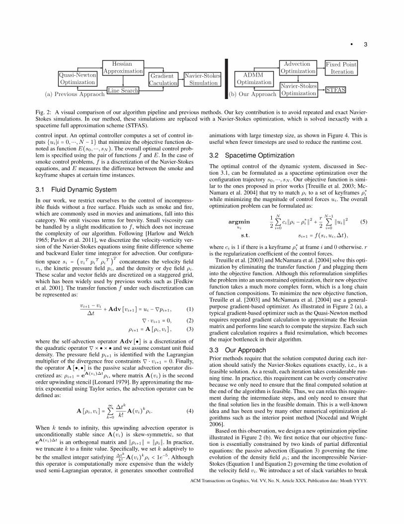
Fig. 2: A visual comparison of our algorithm pipeline and previous methods. Our key contribution is to avoid repeated and exact Navier-Stokes simulations. In our method, these simulations are replaced with a Navier-Stokes optimization, which is solved inexactly with aspacetime full approximation scheme (STFAS).

control input. An optimal controller computes a set of control in-puts {ui∣i = 0,⋯,N − 1} that minimize the objective function de-noted as function E(s0,⋯, sN). The overall optimal control prob-lem is specified using the pair of functions f and E. In the case ofsmoke control problems, f is a discretization of the Navier-Stokesequations, and E measures the difference between the smoke andkeyframe shapes at certain time instances.

3.1 Fluid Dynamic System

In our work, we restrict ourselves to the control of incompress-ible fluids without a free surface. Fluids such as smoke and fire,which are commonly used in movies and animations, fall into thiscategory. We omit viscous terms for brevity. Small viscosity canbe handled by a slight modification to f , which does not increasethe complexity of our algorithm. Following [Harlow and Welch1965; Pavlov et al. 2011], we discretize the velocity-vorticity ver-sion of the Navier-Stokes equations using finite difference schemeand backward Euler time integrator for advection. Our configura-tion space si = (vi

T piT ρi

T )T

concatenates the velocity fieldvi, the kinetic pressure field pi, and the density or dye field ρi.These scalar and vector fields are discretized on a staggered grid,which has been widely used by previous works such as [Fedkiwet al. 2001]. The transfer function f under such discretization canbe represented as:

vi+1 − vi∆t

+Adv [vi+1] = ui −∇pi+1, (1)

∇ ⋅ vi+1 = 0, (2)ρi+1 =A [ρi, vi] , (3)

where the self-advection operator Adv [●] is a discretization ofthe quadratic operator ∇× ● × ● and we assume constant unit fluiddensity. The pressure field pi+1 is identified with the Lagrangianmultiplier of the divergence free constraints ∇ ⋅ vi+1 = 0. Finally,the operator A [●, ●] is the passive scalar advection operator dis-cretized as: ρi+1 = eA(vi)∆tρi, where matrix A(vi) is the secondorder upwinding stencil [Leonard 1979]. By approximating the ma-trix exponential using Taylor series, the advection operator can bedefined as:

A [ρi, vi] =∞

∑k=0

∆tk

k!A(vi)

kρi. (4)

When k tends to infinity, this upwinding advection operator isunconditionally stable since A(vi) is skew-symmetric, so thateA(vi)∆t is an orthogonal matrix and ∥ρi+1∥ = ∥ρi∥. In practice,we truncate k to a finite value. Specifically, we set k adaptively tobe the smallest integer satisfying ∆tk

k!A(vi)

kρi < 1e−5. Althoughthis operator is computationally more expensive than the widelyused semi-Lagrangian operator, it generates smoother controlled

animations with large timestep size, as shown in Figure 4. This isuseful when fewer timesteps are used to reduce the runtime cost.

3.2 Spacetime Optimization

The optimal control of the dynamic system, discussed in Sec-tion 3.1, can be formulated as a spacetime optimization over theconfiguration trajectory s0,⋯, sN . Our objective function is simi-lar to the ones proposed in prior works [Treuille et al. 2003; Mc-Namara et al. 2004] that try to match ρi to a set of keyframes ρ∗iwhile minimizing the magnitude of control forces ui. The overalloptimization problem can be formulated as:

argminui

1

2

N

∑i=0

ci∥ρi − ρ∗

i ∥2+r

2

N−1

∑i=0

∥ui∥2 (5)

s.t. si+1 = f(si, ui,∆t),

where ci is 1 if there is a keyframe ρ∗i at frame i and 0 otherwise. ris the regularization coefficient of the control forces.

Treuille et al. [2003] and McNamara et al. [2004] solve this opti-mization by eliminating the transfer function f and plugging theminto the objective function. Although this reformulation simplifiesthe problem into an unconstrained optimization, their new objectivefunction takes a much more complex form, which is a long chainof function compositions. To minimize the new objective function,Treuille et al. [2003] and McNamara et al. [2004] use a general-purpose gradient-based optimizer. As illustrated in Figure 2 (a), atypical gradient-based optimizer such as the Quasi-Newton methodrequires repeated gradient calculation to approximate the Hessianmatrix and performs line search to compute the stepsize. Each suchgradient calculation requires a fluid resimulation, which becomesthe major bottleneck in their algorithm.

3.3 Our ApproachPrior methods require that the solution computed during each iter-ation should satisfy the Navier-Stokes equations exactly, i.e., is afeasible solution. As a result, each iteration takes considerable run-ning time. In practice, this requirement can be overly conservativebecause we only need to ensure that the final computed solution atthe end of the algorithm is feasible. Thus, we can relax this require-ment during the intermediate steps, and only need to ensure thatthe final solution lies in the feasible domain. This is a well-knownidea and has been used by many other numerical optimization al-gorithms such as the interior point method [Nocedal and Wright2006].

Based on this observation, we design a new optimization pipelineillustrated in Figure 2 (b). We first notice that our objective func-tion is essentially constrained by two kinds of partial differentialequations: the passive advection (Equation 3) governing the timeevolution of the density field ρi; and the incompressible Navier-Stokes (Equation 1 and Equation 2) governing the time evolution ofthe velocity field vi. We introduce a set of slack variables to break


4 ●

these two kinds of constraints into two subproblems: AdvectionOptimization ( AO ) is constrained only by Equation 3 and Navier-Stokes Optimization ( NSO ) is constrained only by Equation 1 andEquation 2. In order to solve the Advection Optimization (Sec-tion 4.1), we use a fixed point iteration defined for its KKT condi-tions. For the Navier-Stokes Optimization (Section 4.2), we updateour solution using a spacetime full approximation scheme (STFAS)to avoid repeated fluid resimulations. This can lead to great speedupnot only because of the fast convergence of a multigrid solver, butalso because the multigrid solver allows warm-starting, so that wecan make use of the coherence between consecutive iterations. Incontrast, previous methods use fluid resimulations, which alwayssolve Navier-Stokes equations from scratch, and solve them ex-actly.

4. SPACETIME OPTIMIZATION USING STFAS

In this section, we present our novel algorithm to solve Equation 5.We also describe our new acceleration method, STFAS. See [No-cedal and Wright 2006] for an introduction to some notations andreference solvers used in this section.

By introducing a series of slack variables v∗i , we can decomposethe overall optimization problem into two subproblems and refor-mulate Equation 5 as:

argminui

1

2

N

∑i=0

ci∥ρi − ρ∗

i ∥2+r

2

N−1

∑i=0

∥ui∥2+

λTi (vi − v∗

i ) +K

2

N−1

∑i=0

∥vi − v∗

i ∥2 (6)

s.t.vi+1 − vi

∆t+Adv [vi+1] = ui −∇pi+1

ρi+1 =A [ρi, v∗

i ] , ∇ ⋅ vi = 0,

where we added the augmented Lagrangian term λTi (vi − v∗

i ) andthe penalty term K

2 ∑N−1i=0 ∥vi − v

∗

i ∥2. This kind of optimization

can be solved efficiently using the well-known alternating direc-tion method of multipliers (ADMM) [Boyd et al. 2011], which hasbeen used in [Gregson et al. 2014] for fluid tracking. Specifically,in each iteration of our algorithm, we first fix vi, pi and solve forv∗i . This subproblem is denoted as the Advection Optimization (AO ) because the PDE constraints are just a passive advection ofthe density field ρi. We then fix v∗i and solve for vi, pi. We de-note this subproblem as the Navier-Stokes Optimization ( NSO), constrained by the incompressible Navier-Stokes equations. Thefinal step is to adjust λi according to the constraint violation as:λi = λi +Kβ(vi − v

∗

i ) where β is a constant parameter.The advantage of breaking the problem up is that we can derive

simple and effective algorithms to solve each subproblem. Our al-gorithm directly solves the first order optimality (KKT) conditionsof both problems. To solve the AO subproblem, we introduce afixed point iteration in Section 4.1, while for the NSO subprob-lem, which is the bottleneck of the algorithm, we introduce STFASsolver in Section 4.2.

4.1 Advection Optimization

The goal of solving the AO subproblem is to find a sequence ofvelocity fields v∗i to advect ρi so that it matches the keyframes,assuming that these v∗i are uncorrelated. By dropping terms irrel-evant to v∗i from Equation 6, we get a concise formulation for the

AO subproblem:

argminv∗i

1

2

N

∑i=0

∥ρi − ρ∗

i ∥2Ci+K

2

N−1

∑i=0

∥vi − v∗

i ∥2 (7)

s.t. ρi+1 =A [ρi, v∗

i ] ∇ ⋅ v∗i = 0,

where we have absorbed the augmented Lagrangian term λTi (vi −v∗i ) by setting: vi = vi + λi/K.

Due to the inherent nonlinearity and ambiguity in the advectionoperator, an AO solver is prone to falling into local minimum, lead-ing to trivial solutions. We introduce two additional modificationsto Equation 7 to avoid these trivial solutions. First, we replace thescalar coefficient ci with a matrix Ci which could be used to avoidthe problem of a zero gradient if the keyframe ρ∗i is far from thegiven density field ρi. Similar to [Treuille et al. 2003; Fattal andLischinski 2004], we take Ci = ciΣiGTi Gi to be a series of Gaus-sian filters Gi with receding support. Specifically, Gi has a stan-dard deviation σ(Gi) = 2σ(Gi−1). The combination of these filtersspreads the gradient information throughout the domain. Moreover,the keyframe features of various frequencies get equally penalized.We also introduce additional solenoidal constraints on v∗i . Note thatthis term does not alter the optima of Equation 6 since vi = v∗ion convergence. However, it prevents the optimizer from creatingor removing densities in order to match the keyframe, which is atempting trivial solution.

We solve this optimization via a fixed point iteration derivedfrom its KKT conditions. To derive this system we introduceLagrangian multipliers µi for each advection equation ρi+1 =

A [ρi, v∗

i ] and γi for the solenoidal constraints, giving a La-grangian function:

L =1

2

N

∑i=0

∥ρi − ρ∗

i ∥2Ci+K

2

N−1

∑i=0

∥vi − v∗

i ∥2+

N−1

∑i=0

µTi (ρi+1 −A [ρi, v∗

i ]) + γTi ∇ ⋅ v∗i .

After taking the derivative of the above Lagrangian against ρi, v∗i(primal variables) and µi, γi (dual variables), respectively, we getthe following set of KKT conditions for 0 ≤ i ≤ N :

µi−1 =∂A [ρi, v

∗

i ]

∂ρi

T

µi −Ci(ρi − ρ∗

i )

v∗i−1 =Q(vi−1 +∂A [ρi−1, v

∗

i−1]

∂v∗i−1

Tµi−1

K) (8)

ρi+1 −A [ρi, v∗

i ] = 0, ∇ ⋅ v∗i = 0,

where we set µ−1 = µN = 0 to unify the index, and we have re-placed γi with a solenoidal projection operator Q. This actuallydefines a fixed point iteration where we can first update ρi in a for-ward pass and then update µi, vi in a backward pass. This is closelyrelated to the adjoint method [McNamara et al. 2004], which alsotakes a forward-backward form. Unlike [McNamara et al. 2004]which then solves v∗i using quasi-Newton method, a fixed pointiteration is much simpler to implement, and a general-purpose op-timizer is not needed. The mostly costly step in applying Equa-tion 8 is the operator Q where we use conventional multigrid Pois-son solver [Trottenberg and Schuller 2001]. A pseudo-code of ourAO solver is given in Algorithm 1.

In the above derivation, since we do not exploit any structure inthe operator A [ρi, v

∗

i ], basically any advection operator other thanEquation 4, such as semi-Lagrangian, could be used as long as its


● 5

Algorithm 1 The Fixed Point Iteration: This is used to solve theAO subproblem. The algorithm consists of a forward sweep thatupdates the density fields ρi and a backward sweep that updates µiand vi.

Input: Initial vi, ρ0 and keyframes ρ∗iOutput: Fixed point vi, µi

1: for i = 0,⋯,N − 1 do2: ▷ Initialization3: v∗i = vi4: end for5: for i = 1,⋯,N do6: ▷ Find primal variable ρ7: ρi =A [ρi−1, v

∗

i−1]

8: end for9: set µ−1 = µN = 0

10: for i = N,⋯,1 do11: ▷ Find dual variable µ

12: µi−1 =∂A[ρi,v

∗

i ])

∂ρi

T

µi −Ci(ρi − ρ∗

i )

13: ▷ Find primal variable v

14: v∗i−1 =Q(vi−1 +∂A[ρi−1,v

∗

i−1])

∂v∗i−1

Tµi−1K

)

15: end for

t = 3s t = 6s t = 9s t = 12s

Fig. 4: We tested the fixed point iteration Equation 8 using different ad-vection operator A [●, ●] to deform an initially circle-shaped smoke (topleft) into the bird icon (bottom left). The AO subproblem solved using thesemi-Lagrangian operator involves lots of popping artifacts (top row). Theupwinding operator in Equation 4 doesn’t suffer from such problems (bot-tom row).

partial derivatives against ρi, v∗i are available. Empirically, how-ever, Equation 4 generally gives smoother animations especiallyunder large timestep size. This is because the semi-Lagrangian op-erator can jump across multiple cells when performing backtrack-ing, and the density value changes in these cells are ignored. As aresult, the semi-Lagrangian operator suffers from popping artifactsas illustrated in Figure 4, while our operator (Equation 4), beingpurely grid-based, doesn’t exhibit such problem. Unlike [Treuilleet al. 2003], where these popping artifacts can be alleviated by con-straining control force fields to a small set of force templates, weallow every velocity component to be controlled. In this case, theuse of our new advection operator is highly recommended.

4.2 Navier-Stokes Optimization

Complementary to Section 4.1, the goal of the Navier-Stokes Opti-mization is to enforce the correlation between vi given the sequenceof guiding velocity fields v∗i . The optimization takes the following

form:

argminvi

r

2

N−1

∑i=0

∥ui∥2+K

2

N−1

∑i=0

∥vi − v∗

i ∥2

s.t.vi+1 − vi

∆t+Adv [vi+1] = ui −∇pi+1

∇ ⋅ vi = 0.

This subproblem is the bottleneck of our algorithm, for which aforward-backward adjoint method similar to Equation 8 requiressolving the Navier-Stokes equations exactly in the forward pass. Toavoid this costly solve, we update primal as well as dual variablesin a single unified algorithm. In the same way as in Section 4.1, wederive the KKT conditions and assemble them into a set of nonlin-ear equations:

f =

⎛⎜⎜⎜⎝

Kr(vi − v

∗

i ) +∂ui∂vi

Tui +

∂ui−1∂vi

Tui−1 +∇pi

∇ ⋅ vivi+1−vi

∆t+Adv [vi+1] − ui +∇pi+1

∇ ⋅ ui

⎞⎟⎟⎟⎠

= 0, (9)

where the partial derivatives are ∂ui∂vi

= − I∆t

, ∂ui−1∂vi

= I∆t

+

∂Adv[vi]

∂vi, and the additional variable pi is the Lagrangian multi-

plier for the solenoidal constraint: ∇ ⋅ vi = 0. We refer readers toAppendix A for the derivation of Equation 9. In summary, we haveto solve for the primal variables ui, vi as well as the dual variablespi, pi. Unlike Equation 8, however, we do not differentiate thesetwo sets of variables and solve for them by iteratively bringing theresidual f to zero.

i =Ni = 0

R P

STagging

Spatial Resolution

Tim

este

pIn

dex

i

Fig. 5: A 2D illustration of our STFAS multigrid scheme. We use semi-coarsening only in the spatial direction (horizontal), with each finer leveldoubling the grid resolution. We use trilinear interpolation operators forP,R and tridiagonal SCGS smoothing for S, which solves the primal vari-ables vi, ui (defined on faces as short white lines) and dual variables pi, pi(defined in cell centers as black dots) associated with one cell across all thetimesteps (vertical) by solving a block tridiagonal system. The solve can bemade parallel by the 8 − color tagging in 3D or 4 − color tagging in 2D.

To this end, we develop a spacetime full approximation scheme(STFAS), which is a geometric multigrid algorithm designed forsolving a nonlinear system of equations as illustrated in Figure 5.The multigrid solver is a classical tool originally used for solvinglinear systems induced from elliptical PDEs. We refer the readers


6 ●

to [Trottenberg and Schuller 2001] for a detailed introduction andbriefly review the core idea here.

4.3 STFAS Algorithm

Our multigrid solver works on a hierarchy of grids in descend-ing resolutions. In each STFAS iteration, it refines the solution(vi, pi, ui, pi) by reducing the residual f(vi, pi, ui, pi). Since dif-ferent components of the residual can be reduced most effectively atdifferent resolutions, the multigrid solver downsamples the residualto appropriate resolutions and then upsamples and combines theirsolutions. With properly defined operators introduced in this sec-tion, our multigrid algorithm can generally achieve a linear rate oferror reduction, which is optimal in the asymptotic sense.

To adopt this idea to solve Equation 9, we introduce a hier-archy of spacetime grids (vhi , p

hi , u

hi , p

hi ), where h is the cell

size. We use semi-coarsening in spatial direction only where everycoarser level doubles the cell size. We denote the coarser level as(v2hi , p2h

i , u2hi , p

2hi ). We use the simple FAS-VCycle(2,2) iteration

to solve the nonlinear system of equations: f(vi, pi, ui, pi) = res.See Algorithm 2 for details of the NSO solver.

Algorithm 2 STFAS VCycle(vhi , phi , u

hi , p

hi , res

h): This is used

to solve the NSO subproblem. The algorithm is a standard FASVCycle with 2 pre and post smoothing (Line 8, Line 28) and 10final smoothing (Line 3).

Input: A tentative solution (vhi , phi , u

hi , p

hi )

Output: Refined solution to f(vhi , phi , u

hi , p

hi ) = resh

1: if h is coarsest then2: ▷ Final smoothing for the coarsest level3: for k = 1,⋯,10 do4: S(vhi , p

hi , u

hi , p

hi )

5: end for6: else7: ▷ Pre smoothing8: for k = 1,2 do9: S(vhi , p

hi , u

hi , p

hi )

10: end for11: ▷ Down-sampling12: for t = v, p, u, p and ∀i do13: t2hi =R(thi )

14: thi = thi −P(t2hi )

15: end for16: ▷ Compute FAS residual by combining:17: ▷ 1. the solution on coarse resolution18: ▷ 2. the residual on fine resolution19: res2h

= f(v2hi , p2h

i , u2hi , p

2hi )

20: res2h= res2h

+R(resh − f(vhi , phi , u

hi , p

hi ))

21: ▷ VCycle recursion22: VCycle(v2h

i , p2hi , u

2hi , p

2hi , res

2h)

23: ▷ Up-sampling24: for t = v, p, u, p and ∀i do25: thi = t

hi +P(t2hi )

26: end for27: ▷ Post smoothing28: for k = 1,2 do29: S(vhi , p

hi , u

hi , p

hi )

30: end for31: end if

-8

-7

-6

-5

-4

-3

-2

-1

0

1 9

17

25

33

41

49

57

65

73

81

89

97

10

5

11

3

12

1

12

9

13

7

14

5

15

3

16

1

16

9

17

7

18

5

Log

Rel

ativ

e K

KT

Res

idu

al

#STFAS VCycle

LBFGS 64^3/128 LBFGS 128^3/256STFAS 64^3/128 STFAS 128^3/256

Fig. 6: Convergence history of STFAS compared with that of the LBFGSoptimizer, running on two grid resolutions and with a different number oftimesteps (denoted as nd/N ). STFAS achieves a linear rate of error reduc-tion independent of grid resolution and number of timesteps, as the twocurves overlap.

The fast convergence of the geometric FAS relies on a properdefinition of the three application-dependent operators: R,P andS. The restriction operator R downsamples a fine grid solution to acoarser level for efficient error reduction, and the prolongation op-erator P upsamples the coarse grid solution to correct the fine gridsolution. We use simple trilinear interpolation for these two oper-ators whether applied on scalar or vector fields. Finally, designingthe smoothing operator S is much more involved. S should, by it-self, be a cheap iterative solver for f(vi, pi, ui, pi) = res. Com-pared with previous works such as [Chentanez and Muller 2011]where multigrid is used for solving the pressure field pi only, weare faced with two new challenges. First, since we are solving theprimal as well as dual variables, which gives a saddle point prob-lem, the Hessian matrix is not positive definite in the spatial do-main, so that a Jacobi or Gauss-Seidel (GS) solver does not work.Second, we are not coarsening in the temporal domain, so the tem-poral correlation must be considered in the smoothing operator.

Our solution is to consider the primal and dual variables at thesame time using the Symmetric Coupled Gauss-Seidel (SCGS)smoothing operator [Vanka 1983]. SCGS smoothing is a primal-dual variant of GS. In our case, where all the variables are stored ina staggered grid, SCGS smoothing considers one cell at a time. Itsolves the primal variables vi, ui stored on the 6 cell faces as wellas the dual variables pi, pi stored in the cell center at the same timeby solving a small 14×14 linear problem (10×10 in 2D). Like red-back-GS smoothing, we can parallelize SCGS smoothing using the8-color tagging (see Figure 5).

The above SCGS solver only considers one timestep at a time.To address the second problem of temporal correlation, we augmentthe SCGS solver with the temporal domain. We solve the 14 vari-ables associated with a single cell across all the timesteps at once.Although this involves solving a large 14N × 14N linear systemfor each cell, the left hand side of the linear system is a block tridi-agonal matrix so that we can solve the system in O(N). Indeed,


● 7

the Jacobian matrix of f takes the following form:

∂f∂vi,pi,ui,pi

=

⎛⎜⎜⎜⎜⎜⎜⎜⎜⎜⎜⎜⎜⎝

KrI ∇

∂u0∂v0

T

∇T

∂u0∂v0

−I ∇∂u0∂v1

∇T

∂u0∂v1

T KrI ∇

∇T

⋱

⎞⎟⎟⎟⎟⎟⎟⎟⎟⎟⎟⎟⎟⎠

, (10)

where the size of each block is 5 × 5 in 2D and 7 × 7 in 3D. Dueto this linear time solvability, the optimal multigrid performance isstill linear in the number of spatial-temporal variables. The aver-age convergence history for our multigrid solver is compared witha conventional LBFGS algorithm [McNamara et al. 2004] in Fig-ure 6. Our algorithm achieves a stable linear rate of error reduc-tion independent of both the grid resolution and the number oftimesteps.

4.4 ADMM Outer Loop

Equipped with solvers for the two subproblems, we present ourADMM outer loop in Algorithm 3. We find it difficult for eitherEquation 8 or a quasi-Newton method solving the AO subproblemto converge to an arbitrarily small residual due to the non-smoothnature of the operator A [●, ●]. Both algorithms decrease the objec-tive function in the first few iterations and then wander around theoptimal solution. In view of this, we run Equation 8 (Section 4.1)for a fixed number of iterations before moving on to the NSO sub-problem (Section 4.2) so that each ADMM iteration has O(ndN)

complexity and is linear in the number of spacetime variables. Fi-nally our stopping criterion for the NSO subproblem is that theresidual ∥f∥∞ < εSTFAS . Our stopping criterion for the ADMMouter loop is that the maximal visual difference, the largest differ-ence of the density field over all the timesteps, generated by twoconsecutive ADMM iterations should be smaller than εADMM .

Algorithm 3 ADMM Outer Loop

Input: Parameters K,r, ρ∗i , εSTFAS , εADMM

Output: Optimized velocity fields vi and density fields ρi1: for i = 0,⋯,N do2: Set vi = 03: Set ρlasti = ρi4: end for5: while true do6: ▷ Solve the AO subproblem7: Run Algorithm 1 for a fixed number of iterations8: ▷ Solve the NSO subproblem9: while f(vi, pi, ui, pi) > εSTFAS do

10: Algorithm 211: end while12: ▷ Stopping criterion13: if maxi∥ρ

lasti − ρi∥∞ < εADMM then

14: Return vi, ρi15: end if16: for i = 0,⋯,N do17: Set ρlasti = ρi18: ▷ Update augmented Lagrangian multiplier19: Set λi = λi +Kβ(vi − v∗i )20: end for21: end while

5. RESULTS AND ANALYSIS

Name Value

∆t 0.4 ∼ 2.0sK 103

r 102∼4

β for updating λi 1#Equation 8 2εSTFAS 10−5

εADMMρmax

100

Table I. : Parameters.

Parameter Choice: We usethe same set of parameterslisted in Table I for all exper-iments, where ρmax is themaximal density magnitudeat the initial frame. Underthis setting, the convergencehistory of the ADMM outerloop of our first exampleFigure 1 is illustrated in Fig-ure 7. In our experiments,the ADMM algorithm al-ways converges in fewerthan 50 iterations. Further,

running only 2 iterations of Equation 8 in each ADMM loop willnot deteriorate the performance. In fact, according to the averagedconvergence history of the AO subproblem illustrated in Figure 7,the fixed point iteration Equation 8 usually converges in the first4 iterations before it wanders around a local minimum. After finetuning, we found that 2 iterations lead to the best overall perfor-mance. In this case, the overhead of solving the AO subproblem ismarginal compared with the overhead of solving the NSO subprob-lem. Finally, unlike fluid simulation, the performance of spacetimeoptimization doesn’t depend on the timestep size due to our robustadvection operator (Equation 4). When we increase the timestepsize from 0.4s to 2s for the examples in Figure 8 and Figure 9,which is extremely large, our algorithm’s convergence behavior isabout the same.

-7

-6

-5

-4

-3

-2

-1

0

1 3 5 7 9 1113151719212325272931

Log

Rel

ativ

e K

KT

Res

idu

al

#ADMM Outer Loops200

#ADMM Outer Loops

0

50

100

150

200

1 2 3 4 5 6 7 8 9 10 11 12R

elat

ive

KK

T R

esid

ual

#Fixed Point Iterations

Fig. 7: We profile the convergence history of the example Figure 1. We plotthe logarithm of relative KKT residual of the optimized velocity field aftereach ADMM loop (left); and the absolute residual of the AO subproblem’sKKT conditions after each iteration of Equation 8 (right).

Benchmarks: To demonstrate the efficiency and robustness ofour algorithm, we used 7 benchmark problems that vary in theirgrid resolution, number of timesteps, and number of keyframes.The memory overhead and computational overhead are summa-rized in Table II. All of the results are generated on a desktop PCwith an i7-4790 8-core CPU 3.6GHz and 12GB of memory. We useOpenMP for multithread parallelization.

Our first example is five controlled animations matching a circleto the letters “FLUID”. Compared with [Treuille et al. 2003], whichuses a relatively small set of control force templates to reduce thesearch space of control forces, we allow control on every velocitycomponent so that the matching to keyframe is almost exact. Afterthe keyframe, we remove the control force, and rich smoke detailsare generated by pure simulation as illustrated in Figure 1. How-ever, in the controlled phase of Figure 1, this example seems “toomuch controlled”, meaning that most smoke-like behaviors are lost.This effect has also been noticed in [Treuille et al. 2003]. However,unlike their method, in which the number of templates needs tobe carefully tuned to recover such behavior, we can simply adjustthe regularization r in our system to balance matching exactnessand the amount of smoke-like behaviors. In Figure 8, we generated


8 ●

Example(nd/N) Boundary #ADMM Avg. AO (s) Avg. NSO (s) Total(hr) Memory(Gb) Total LBFGS(hr)

Letters FLUID(1282/40, r = 103

) Neumann 13 10 60 0.25 0.06 4Circle Bunny(1282

/80, r = 102) Neumann 25 20 130 1.04 0.2 12

Circle Bunny(1282/80, r = 103

) Neumann 37 20 220 2.46 0.2 15Circle Bunny(1282

/80, r = 104) Neumann 43 20 218 2.84 0.2 16

Letters ABC(1282/60, r = 104

) Neumann 33 16 179 1.78 0.15 14Sphere Armadillo Bunny(643

/40, r = 103) Neumann 17 103 1341 6.81 1.34 N/A

Varying Genus(642× 32/40, r = 103

) Periodic 20 82 840 5.12 0.67 N/AHuman Mocap(642

× 128/60, r = 103) Periodic 5 1437 3534 6.9 4.0 N/A

Moving Sphere(643/60, r = 102

) Neumann 17 630 1792 11.43 2.2 N/AMoving Sphere(643

/60, r = 103) Neumann 22 630 1978 15.93 2.2 N/A

Table II. : Memory and computational overhead for all the benchmarks. From left to right: name of example (resolution parameters); thespatial boundary condition; number of outer ADMM iterations; average time spent on each AO subproblem; average time spent on each NSOsubproblem; total time until convergence using our algorithm; memory overhead; total time until convergence using LBFGS. By comparingthe three “Circle Bunny” examples, we can see that the number of ADMM outer loops is roughly linear to log10(r). More ADMM outerloops are needed, if more fluid-like behaviors are desired. And the computational cost of each ADMM outer loop is roughly linear in thenumber of timesteps. This can be verified by comparing the “Letters FLUID” and the “Circle Bunny” example.

Fig. 8: For this animation, we match the circle (red) first to two smallercircles and then to a bunny (we show frames 20,40,60,80 from top tobottom). The resolution is 1282/80, and we test three different values ofghost force regularization r = 102,3,4 (from left to right). More smoke-likebehaviors are generated as we increase r.

Fig. 9: In this example, we deform a sphere into letter “A”, then letter “B”and finally letter “C”. For such complex deformation, it is advantageous toallow every velocity component to be optimized. So that a lot of fine-scaledetails can be generated as illustrated in the white circles.

three animations with two keyframes: first two circles and then abunny, using r = 102,3,4 respectively. These animations are alsoshown in the video. Our algorithm is robust to a wide range of pa-rameter choices. But more iterations are needed for the multigrid toconverge for a larger r as shown in Table II. Finally, since we allowevery velocity component to be optimized, the resulting animationexhibits lots of small-scale details as indicated in Figure 9, which isnot possible with the small set of force templates used in [Treuilleet al. 2003].

In addition to these 2D examples, we also tested our algorithmon some 3D benchmarks. Our first example is shown in Figure 10and runs at a resolution of 643

/40. We use two keyframes at frame20 and 40, and the overall optimization takes about 7 hours. In oursecond example, shown in Figure 11, we try to track the smokewith a dense sequence of keyframes from the motion capture dataof a human performing a punch action. Such an example is con-sidered the most widely used benchmarks for PD-type controllerssuch as [Shi and Yu 2005]. With such strong and dense guidance,our algorithm converges very quickly, within 5 iterations. Our thirdexample (Figure 13) highlights the effect of regularization coeffi-cient r in 3D. Like our 2D counterpart Figure 8, larger r usually re-sults in more wake flow behind moving smoke bodies. Finally, weevaluated our algorithm on a benchmark with keyframe shapes ofvarying genera. As illustrated in Figure 12, the initial smoke shapehas genus zero, but we use two keyframes, where the smoke shapeshave genus one and two. Our algorithm can handle such complexcases.

Comparison with LBFGS: We compared our algorithm witha gradient-based quasi-Newton optimizer. Specifically, we useLBFGS method [Nocedal and Wright 2006]. Such method approx-imates the Hessian using a history of gradients calculated by pastiterations. We set the history size to be 8, which is typical. We usesame stopping criteria for both LBFGS and our method. Under thissetting, we compared the performance of LBFGS and the ADMMsolver on two of our 2D examples: Figure 1 and Figure 8. For theexample of letter matching in Figure 1, LBFGS algorithm takes 4hrand 71 iterations to converge. While for the example of changingregularization in Figure 8, LBFGS algorithm takes 12hr and 152iterations at r = 102, 15hr and 170 iterations at r = 103, and 16hrand 212 iterations at r = 104. Therefore, our algorithm is approxi-mately an order of magnitude faster than a typical implementationof LBFGS.


● 9

Fig. 10: 3D smoke control example of deforming a sphere first to an armadillo and then to a bunny. This example runs at the resolution of643 with 40 timesteps. The optimization can be accomplished in 7hr.

Fig. 11: We generate the famous example of tracking smoke with a dense sequence of keyframes, which comes from human motion capturedata. Our algorithm converges and generates rich smoke drags within 5 ADMM iterations.

The speedup over LBFGS optimizer occurs for two reasons.First, we break the problem up into the AO subproblem and theNSO subproblem, that have sharply different properties. The AOsubproblem is nonsmooth while the NSO subproblem is not. Inpractice, neither our fixed point iteration scheme in Equation 8 northe LBFGS algorithm can efficiently solve AO to arbitrarily smallKKT residual. Without such decomposition, it takes a very longtime to solve the overall optimization problem by taking a lot ofiterations. The second reason is the use of warm-started STFASsolver for the NSO subproblem. Note that LBFGS algorithm notonly takes more iterations, but each iteration is also more expen-sive. This is mainly because of the repeated gradient evaluationin each LBFGS iteration, where each evaluation runs the adjointmethod with a cost equivalent to two passes of fluid resimulation.

Comparison with PD Controller: We also compared ourmethod with simple tracker type controllers such as PD controller[Fattal and Lischinski 2004]. To drive the fluid body towards a tar-get keyframe shape using heuristic ghost forces, PD controllers re-sult in much lower overhead in terms of fluid resimulation, as com-pared to our approach based on optimal controllers. In contrast,optimal controllers provide better flexibility and robust solutions ascompared to PD controllers. A PD controller tends to be very sensi-tive to the parameters of the ghost force. Moreover, its performancealso depends on the non-physical gathering term to generate plausi-ble results (see Figure 15). On the other hand, an optimal controllercan achieve exact keyframe timing, which may not be possible us-ing a PD controller, as shown in Figure 15. Moreover, an optimalcontroller can easily balance between the exactness of keyframematching and the amount of fluid-like behavior based on a singletuning parameter r (see Figure 8).

Memory Overhead: Since fluid control problems usually havea high memory overhead, we derive here an analytical upper boundof the memory consumption M(n, d,N):

M(n, d,N) ∼ [(nd) ∗ (1 + d) ∗ 2 ∗ 2] ∗ [1 + 12+ 1

4⋯] ∗N = 8nd(1 + d)N,

where n is the grid resolution, d is the dimension, and N is thenumber of timesteps. To derive this bound, note that we can reuse

the memory consumed by Algorithm 2 in Algorithm 1, and Algo-rithm 2 always consumes more memory than Algorithm 1, so thatwe only consider the memory overhead of Algorithm 2. The firstterm nd ∗ (1 + d) is the number of variables needed for storinga pair of pressure and velocity fields. This number is doubled be-cause we need to store ui, pi in addition to vi, pi at each timestep.We double it again because we need additional memory for stor-ing res in STFAS. Finally, the power series is due to the hierarchyof grids. At first observation, this memory overhead is higher than[Treuille et al. 2003; McNamara et al. 2004] since we require ad-ditional memory for storing the dual variables at multiple resolu-tions. However, due to the quasi-Newton method involved in theirapproach, additional memories are needed to store a set of L gradi-ents to approximate the inverse of the Hessian matrix. L is usually5 ∼ 10, leading to the following upper bound:

MLBFGS(n, d,N) ∼ [(nd) ∗ (1 + d)] ∗L ∗N = Lnd(1 + d)N.

In our benchmarks, the memory overheads of our ADMM andLBFGS solvers are comparable.

Convergence Analysis: Here we analyze the convergence ofour approach and propose some modifications to guarantee con-vergence of iterations used in Algorithm 3.

For our AO solver (Line 7 of Algorithm 3), we observe that itcan be difficult for Algorithm 1 to converge to an arbitrarily smallKKT residual in each loop of Algorithm 3. Although our choice isto perform a fixed number of iterations of Algorithm 1, one couldalso use a simple strategy that can guarantee that function valuedecreases by blending a new solution with the previous solutionand tuning the blending factor in a way similar to the line searchalgorithm. This modification has low computational overhead sinceone doesn’t need to apply the costly solenoidal projection operatorQ again after the blending, as the sum of two solenoidal vectorfields is still solenoidal. In our benchmarks, this strategy leads toa convergent algorithm with low overhead, but the error reductionrate after the first few iterations can be slow.

The same analysis can also be used for the NSO solver (Line 9of Algorithm 3) as well. To ensure convergence of Algorithm 2,


10 ●

Fig. 12: Example of smoke control where the keyframes have varying genera. The initial frame is a sphere (genus 0). The first keyframelocated at frame 20 is a torus (genus 1) and the second keyframe located at frame 40 is the shape eight (genus 2). The resolution is 642

×32/40and the overall optimization takes 5hr with r = 103.

fram

e=0

frame=20

fram

e=40

frame=60

Fig. 13: A moving smoke sphere guided by the 3 keyframes (left). We experimented with r = 103 (top) and r = 104 (bottom). Largerregularization results in more wake flow behind moving smoke bodies. The same effect can be observed in Figure 8.

-4

-3

-2

-1

0

1 6

11

16

21

26

31

36

41

46

51

56

61

66

71

76

81

86

91

96

10

1

10

6

11

1

11

6

12

1

12

6

13

1

r=10e5 r=10e6 r=10e7

#STFAS VCycle

Rel

ativ

eK

KT

Res

idu

al

Fig. 14: Convergence history of the NSO solver in the Circle Bunny ex-ample. When the regularization coefficient r is extremely large, we have totreat the FAS-Vcycle as a subproblem solver of the LM algorithm. In eachsubproblem solve, the convergence rate of FAS-VCycle is still linear.

we could add a perturbation to the penalty coefficient K in theHessian matrix Equation 10. Note that as K → ∞, vi → v∗i .Therefore, this strategy essentially makes Algorithm 2 the subprob-lem solver for the Levenberg-Marquardt algorithm [Nocedal andWright 2006], which in turn guarantees convergence. As illustratedin Figure 14, Levenberg-Marquardt modification can be necessarywhen one uses larger regularization r, because we observe that theconvergence rate decreases as r increases.

Finally, for the ADMM outer loop (Line 5 of Algorithm 3), cur-rent analysis of its convergence relies on strong assumptions of itsobjective function, such as global convexity. However, ADMM, asa variant of the Augmented Lagrangian solver [Nocedal and Wright2006], is guaranteed to converge by falling back to a standard Aug-mented Lagrangian solver. Specifically, one can run Algorithm 3without applying Line 18 until the decrease in function value islower than some threshold.

We have applied the above modifications for Line 7 and Line 9of Algorithm 3, which then takes a slightly more complex form.However, the introduced computational overhead is marginal.

6. CONCLUSION AND LIMITATIONS

In our work, we present a new algorithm for the optimal control ofsmoke animation. Our algorithm finds the stationary point of theKKT conditions, solving for both primal and dual variables. Ourkey idea is to refine primal as well as dual variables in a warm-started manner, without requiring them to satisfy the Navier-Stokesequations exactly in each iteration. We tested our approach on sev-eral benchmarks and a wide range of parameter choices. The re-sults show that our method can robustly find the locally optimalcontrol forces while achieving an order of magnitude speedup overthe gradient-based optimizer, which performs fluid resimulation ineach gradient evaluation.

On the downside, our method severely relies on the spatial struc-ture and the staggered grid discretization of the Navier-Stokesequations. This imposes a major restriction to the application ofour techniques. Nevertheless, generalizing our idea to other fluiddiscretization is still possible. For example, our method can be usedwith a fluid solver discretized on a general tetrahedron mesh suchas [Chentanez et al. 2007; Pavlov et al. 2011] since the KKT con-ditions are invariant under different discretizations, and the threeoperators to define STFAS stay valid. On the other hand, general-izing our method to free-surface flow or to handle internal bound-ary conditions can be non-trivial. The distance metric Ci in Equa-tion 7 needs to be modified to make it aware of the boundaries, e.g.,Euclidean distances should be replaced with Geodesic distances.However, modifying the NSO solver to handle the boundaries canbe relatively straightforward. This is because our multigrid formu-lation is the same as a conventional multigrid formulation in spatialdomain, using simple trilinear prolongation and restriction opera-tors. Therefore, existing works on boundary aware multigrid suchas [Chentanez and Muller 2011] can also be applied to our space-time formulation.


● 11

t = 10s

t = 20s

t = 100s

t = 10s

Fig. 15: In order to deform the smoke circle into the bunny, the opti-mal controller achieves exact and reliable keyframe timing and produces asmooth matched shape (top left). But PD-controller requires careful tuningof ghost force coefficient to achieve such exact timing. In addition, thereis still some wandering smoke (white circle) around the keyframe shape(bottom right). If one uses larger ghost force coefficient, the smoke vibratesaround the keyframe and a stable matching occurs 10s later (bottom left),with more wandering smokes (white circle). Moreover, PD-controller relieson the non-physical gathering term to generate plausible results. Withoutthis gathering term, the keyframe is not matched, regardless of the length ofthe animation (top right).

In addition, unlike [Treuille et al. 2003; McNamara et al. 2004],which use a set of template ghost force bases to reduce the searchspace, our method allows every velocity component to be opti-mized. This choice is application dependent. For matching smoketo detailed keyframes with lots of high frequency features, our for-mulation can be useful. However, using a reduced set of templateghost forces could help to avoid the popping artifacts illustrated inFigure 4, and at the same time it allows more user control over theapplied control force patterns. For example, the use of vortex forcetemplates encourages more swirly motions in the controlled anima-tions. Combining the control force templates with our formulationis considered as future work.

In terms of computational overhead, since our optimal controlleralways solves the spacetime optimization by considering all thetimesteps, it is much slower than a simple PD controller which con-siders one timestep at a time. In order to reduce runtime cost, wecan use a larger timestep size to reduce the number of timesteps.Our novel advection operator Equation 4 can robustly handle thissetting. Also, we can lower the spatial resolution in the controlphase and then use smoke upsampling methods such as [Nielsenand Bridson 2011] to generate a high quality animation.

In addition, further accelerations to our method are still possi-ble. For example, parallelization of our algorithm in a distributedenvironment is straightforward. Indeed, multigrid is known as oneof the most cluster-friendly algorithms. Moreover, meta-algorithmssuch as multiple shooting [Bock and Plitt 1984] try to break thespacetime optimization into a series of sub-optimizations that con-sider only a short animation segment and are thus faster to solve. Fi-

nally, we can also combine the benefits of both optimal and PD con-trollers by borrowing the idea of receding horizon control [Mayneand Michalska 1990]. In these controllers, optimal control is ap-plied only to a short window of timesteps starting from the currentone, and the window keeps being shifted forward to cover the wholeanimation.

APPENDIX

A. KKT SYSTEM OF THE NSO SUBPROBLEM

We derive here the KKT system for the NSO subproblem. Insteadof simply introducing the Lagrangian multipliers and followingstandard techniques as we did for the AO subproblem, we presenta derivation based on the analysis of the ghost force ui. We firsteliminate the Navier-Stokes constraints by writing ui as a functionof vi and vi+1. Next, we plug this function into our objective toobtain:

r

2

N−1

∑i=0

∥ui(vi, vi+1)∥2+K

2

N−1

∑i=0

∥vi − v∗

i ∥2.

Taking the derivative of this objective against vi and consideringthe additional solenoidal constraints on vi, we get the first twoequations in f :

K

r(vi − v

∗

i ) +∂ui∂vi

T

ui +∂ui−1

∂vi

T

ui−1 +∇pi = 0

∇ ⋅ vi = 0,

where pi is the Lagrangian multiplier. Now in order to derive theother two conditions in Equation 9, we need to determine the addi-tional pressure pi. We assert that pi+1 is the Lagrangian multiplierof the solenoidal constraints on ui. In fact, if ui is not divergence-free, we can always perform a pressure projection on ui by mini-mizing ∥ui −∇pi+1∥

2 to get a smaller objective function value. Asa result, ui must be divergence-free at the optima with pi+1 beingthe Lagrangian multiplier, and we get the two additional equationsof f :

vi+1 − vi∆t

+Adv [vi+1] − ui +∇pi+1 = 0

∇ ⋅ ui = 0.

From these two conditions, we can see that ∂ui∂vi

= −Q I∆t

, ∂ui−1∂vi

=

Q( I∆t

+∂Adv[vi]

∂vi). Here Q is the solenoidal projection operator

introduced in Equation 8. However, we can drop this Q because wehave ∂ui−1

∂vi

Tui = ( I

∆t+∂Adv[vi]

∂vi)TQTui and QTui =Qui = ui

by the fact that ui is already solenoidal.

REFERENCES

Alexis Angelidis, Fabrice Neyret, Karan Singh, and Derek Nowrouzezahrai.2006. A Controllable, Fast and Stable Basis for Vortex Based SmokeSimulation. In Proceedings of the 2006 ACM SIGGRAPH/EurographicsSymposium on Computer Animation (SCA ’06). Eurographics Associa-tion, 25–32.

Bradley Atcheson, Ivo Ihrke, Wolfgang Heidrich, Art Tevs, Derek Bradley,Marcus Magnor, and Hans-Peter Seidel. 2008. Time-resolved 3d captureof non-stationary gas flows. In ACM transactions on graphics (TOG),Vol. 27. ACM, 132.

Hans Georg Bock and Karl-Josef Plitt. 1984. A multiple shooting algorithmfor direct solution of optimal control problems. Proceedings of the IFACWorld Congress.


12 ●

Alfio Borzi and R Griesse. 2005. Experiences with a space–time multigridmethod for the optimal control of a chemical turbulence model. Interna-tional journal for numerical methods in fluids 47, 8-9 (2005), 879–885.

Stephen Boyd, Neal Parikh, Eric Chu, Borja Peleato, and Jonathan Eckstein.2011. Distributed optimization and statistical learning via the alternatingdirection method of multipliers. Foundations and Trends® in MachineLearning 3, 1 (2011), 1–122.

Nuttapong Chentanez, Bryan E Feldman, Francois Labelle, James FO’Brien, and Jonathan R Shewchuk. 2007. Liquid simulation onlattice-based tetrahedral meshes. In Proceedings of the 2007 ACM SIG-GRAPH/Eurographics symposium on Computer animation. EurographicsAssociation, 219–228.

Nuttapong Chentanez and Matthias Muller. 2011. Real-time eulerian wa-ter simulation using a restricted tall cell grid. In ACM Transactions onGraphics (TOG), Vol. 30. ACM, 82.

T Corpetti, E Memin, and P Perez. 2000. Adaptation of standard optic flowmethods to fluid motion. Citeseer.

Raanan Fattal and Dani Lischinski. 2004. Target-driven smoke animation.In ACM Transactions on Graphics (TOG), Vol. 23. ACM, 441–448.

Ronald Fedkiw, Jos Stam, and Henrik Wann Jensen. 2001. Visual simula-tion of smoke. In Proceedings of the 28th annual conference on Computergraphics and interactive techniques. ACM, 15–22.

James Gregson, Ivo Ihrke, Nils Thuerey, and Wolfgang Heidrich. 2014.From Capture to Simulation: Connecting Forward and Inverse Problemsin Fluids. ACM Trans. Graph. 33, 4, Article 139 (July 2014), 11 pages.DOI:http://dx.doi.org/10.1145/2601097.2601147

F. H. Harlow and J. E. Welch. 1965. Numerical calculation of time-dependent viscous incompressible flowof fluid with free surfaces. Physicsof Fluids 8 (1965), 2182–2188.

Roland Herzog and Karl Kunisch. 2010. Algorithms for PDE-constrainedoptimization. GAMM-Mitteilungen 33, 2 (2010), 163–176.

Michael Hinze, Michael Koster, and Stefan Turek. 2012. A space-timemultigrid method for optimal flow control. In Constrained optimizationand optimal control for partial differential equations. Springer, 147–170.

Ivo Ihrke and Marcus Magnor. 2004. Image-based tomographic re-construction of flames. In Proceedings of the 2004 ACM SIG-GRAPH/Eurographics symposium on Computer animation. EurographicsAssociation, 365–373.

S Kadri-Harouna, Pierre Derian, Patrick Heas, and Etienne Memin. 2013.Divergence-free wavelets and high order regularization. Internationaljournal of computer vision 103, 1 (2013), 80–99.

Brian P Leonard. 1979. A stable and accurate convective modelling pro-cedure based on quadratic upstream interpolation. Computer methods inapplied mechanics and engineering 19, 1 (1979), 59–98.

David Q Mayne and Hannah Michalska. 1990. Receding horizon controlof nonlinear systems. Automatic Control, IEEE Transactions on 35, 7(1990), 814–824.

Antoine McNamara, Adrien Treuille, Zoran Popovic, and Jos Stam. 2004.Fluid control using the adjoint method. In ACM Transactions On Graph-ics (TOG), Vol. 23. ACM, 449–456.

Igor Mordatch, Emanuel Todorov, and Zoran Popovic. 2012. Discovery ofcomplex behaviors through contact-invariant optimization. ACM Trans-actions on Graphics (TOG) 31, 4 (2012), 43.

Michael B Nielsen and Robert Bridson. 2011. Guide shapes for high res-olution naturalistic liquid simulation. In ACM Transactions on Graphics(TOG), Vol. 30. ACM, 83.

Michael B Nielsen and Brian B Christensen. 2010. Improved variationalguiding of smoke animations. In Computer Graphics Forum, Vol. 29. Wi-ley Online Library, 705–712.

Jorge Nocedal and Stephen Wright. 2006. Numerical optimization. SpringerScience & Business Media.

Zherong Pan, Jin Huang, Yiying Tong, Changxi Zheng, and Hujun Bao.2013. Interactive localized liquid motion editing. ACM Transactions onGraphics (TOG) 32, 6 (2013), 184.

Dmitry Pavlov, Patrick Mullen, Yiying Tong, Eva Kanso, Jerrold E Mars-den, and Mathieu Desbrun. 2011. Structure-preserving discretization ofincompressible fluids. Physica D: Nonlinear Phenomena 240, 6 (2011),443–458.

Nick Rasmussen, Doug Enright, Duc Nguyen, Sebastian Marino, NigelSumner, Willi Geiger, Samir Hoon, and Ron Fedkiw. 2004. Di-rectable photorealistic liquids. In Proceedings of the 2004 ACM SIG-GRAPH/Eurographics symposium on Computer animation. EurographicsAssociation, 193–202.

Karthik Raveendran, Nils Thuerey, Chris Wojtan, and Greg Turk. 2012.Controlling liquids using meshes. In Proceedings of the ACM SIG-GRAPH/Eurographics Symposium on Computer Animation. Eurograph-ics Association, 255–264.

Karthik Raveendran, Chris Wojtan, Nils Thuerey, and Greg Turk. 2014.Blending liquids. ACM Transactions on Graphics (TOG) 33, 4 (2014),137.

Lin Shi and Yizhou Yu. 2005. Taming liquids for rapidly changing targets.In Proceedings of the 2005 ACM SIGGRAPH/Eurographics symposiumon Computer animation. ACM, 229–236.

Adrien Treuille, Antoine McNamara, Zoran Popovic, and Jos Stam. 2003.Keyframe control of smoke simulations. ACM Transactions on Graphics(TOG) 22 (2003), 716–723.

Ulrich Trottenberg and Anton Schuller. 2001. Multigrid. Academic Press,Inc., Orlando, FL, USA.

SP Vanka. 1983. Fully coupled calculation of fluid flows with limited use ofcomputer storage. Technical Report. Argonne National Lab., IL (USA).

Xinxin Zhang and Robert Bridson. 2014. A PPPM fast summation methodfor fluids and beyond. ACM Transactions on Graphics (TOG) 33, 6(2014), 206.

Yongning Zhu and Robert Bridson. 2005. Animating sand as a fluid. InACM Transactions on Graphics (TOG), Vol. 24. ACM, 965–972.


http://dx.doi.org/10.1145/2601097.2601147

efﬁcient optimal control of smoke using spacetime multigrid · efﬁcient optimal control of...

Documents