an efficient multigrid method for the simulation of …jteran/papers/zstb10.pdf · an efficient...
TRANSCRIPT
An efficient multigrid method for the simulation of high-resolutionelastic solids
YONGNING ZHU,University of California Los AngelesEFTYCHIOS SIFAKIS, JOSEPH TERANUniversity of California Los Angeles – Walt Disney Animation Studiosand ACHI BRANDTWeizmann Institute of Science
We present a multigrid framework for the simulation of high resolution elas-tic deformable models, designed to facilitate scalability on shared memorymultiprocessors. We incorporate several state-of-the-art techniques frommultigrid theory, while adapting them to the specific requirements of graph-ics and animation applications, such as the ability to handle elaborate ge-ometry and complex boundary conditions. Our method supports simula-tion of linear elasticity and co-rotational linear elasticity. The efficiency ofour solver is practically independent of material parameters, even for near-incompressible materials. We achieve simulation rates as high as 6 framesper second for test models with 256K vertices on an 8-core SMP, and 1.6frames per second for a 2M vertex object on a 16-core SMP.
Categories and Subject Descriptors: I.3.5 [Computer Graphics]: Com-putational Geometry and Object Modeling—Physically based modeling;G.1.8 [Numerical Analysis]: Finite difference methods—Multigrid andmultilevel methods
Additional Key Words and Phrases: Deformable models, co-rotational lin-ear elasticity, near-incompressible solids, parallel simulation
1. INTRODUCTION
Simulation of deformable solids was introduced to computer graph-ics by [Terzopoulos et al. 1987; Terzopoulos and Fleischer 1988].The quest for visual realism has spawned an ever growing interestin simulation techniques capable of accommodating larger, moredetailed models. Several researchers have explored approachessuch as adaptivity [Debunne et al. 2001; Capell et al. 2002; Grin-spun et al. 2002], reduced models [James and Fatahalian 2003;Barbic and James 2005] or shape matching [Muller et al. 2005;Rivers and James 2007] to accelerate the simulation of detailed de-formable models, while others used multi-core platforms [Hugheset al. 2007; Thomaszewski et al. 2007] to reduce simulation times.
Multigrid methods [Trottenberg et al. 2001; Brandt 1977] areamong the fastest numerical solvers for certain elliptic problems.Due to their efficiency, multigrid methods have garnered attentionin the graphics community for a diverse spectrum of applications,including deformable bodies and thin shell simulation [Green et al.2002; Wu and Tendick 2004; Georgii and Westermann 2006; 2008],mesh deformation [Shi et al. 2006], image editing [Kazhdan andHoppe 2008], biomedical simulation [Dick et al. 2008], geometryprocessing [Ni et al. 2004] and in general purpose GPU solvers[Bolz et al. 2003; Goodnight et al. 2003].
We present a scalable framework for fast deformable model sim-ulation based on multigrid techniques. We particularly focus on
the simulation of large models with hundreds of thousands of de-grees of freedom, and aim to create the ideal conditions for ourmethod to scale favorably on shared memory multiprocessors witha large number of cores. In addition, we accommodate models ofarbitrary geometry, and our solver is equally effective even on near-incompressible materials. Although such issues have been individ-ually discussed in the graphics community, we jointly address thechallenges of irregular geometry, near-incompressibilty and par-allel performance without limiting our scope to smaller problemswhich can achieve interactive performance with a broader varietyof techniques. Our solver accommodates the equations of 3D lin-ear (or co-rotational) elasticity as opposed to simpler elliptic sys-tems (e.g. Poisson problems), and performs well for either dynamicor quasistatic simulation. In order to extract the maximum perfor-mance that multigrid formulations have to offer, we adopt some lesscommon choices such as a staggered finite difference discretiza-tion and a mixed formulation of the elasticity equations. We be-lieve these decisions are justified by the performance gains, scala-bility potential and resilience to incompressibility exhibited by ourmethod. Our main contributions are:
—We introduce a novel, symmetric boundary discretization, en-abling robust treatment of irregular geometry and efficientsmoothing of the boundary conditions.
—We show how to accommodate both linear and co-rotational lin-ear elasticity within our framework, for the entire range of com-pressible to highly incompressible materials.
—We demonstrate the mapping and favorable scalability of ourframework on multi-threaded SMP platforms.
2. BACKGROUND
2.1 Linear elasticity
We represent the deformation of an elastic volumetric object usinga deformation function φ which maps any material point X of theundeformed configuration of the object, to its position x in the de-formed configuration, i.e. x = φ(X). Deformation of an objectgives rise to elastic forces [Bonet and Wood 1997] which are ana-lytically given (in divergence form) as f = ∇TP or, component-wise fi =
∑j∂jPij where P is the first Piola-Kirchhoff stress ten-
sor. The stress tensor P is computed from the deformation map φ.This analytic expression is known as the elastic constitutive equa-tion. We will henceforth adopt the common conventions of usingsubscripts after a comma to denote partial derivatives, and omitcertain summation symbols by implicitly summing over any right-hand side indices that do not appear on the left-hand side of a given
ACM Transactions on Graphics, Vol. VV, No. N, Article XXX, Publication date: Month YYYY.
2 • Y. Zhu et al.
equation. Consequently, the previous equation is compactly writtenfi = Pij,j . The constitutive equation of linear elasticity is
P = 2µε+ λtr(ε)I or Pij = 2µεij + λεkkδij (1)
In this equation, µ and λ are the Lame parameters of the linearmaterial, and are computed from Young’s modulus E (a measureof material stiffness) and Poisson’s ratio ν (a measure of materialincompressibility) as µ = E/(2+2ν), λ = Eν/((1+ν)(1−2ν)).Also, δij is the Kronecker delta, ε is the small strain tensor
ε = 12(F + FT )− I or εij = 1
2(φi,j + φj,i)− δij (2)
and F is the deformation gradient tensor, defined as Fij = φi,j .Using (1,2) we derive the governing equations
fi = µφi,jj + (µ+ λ)φj,ij = Lijφj (3)
In this equation L = µ∆I + (µ+ λ)∇∇T is the partial differen-tial operator of linear elasticity. A static elasticity problem amountsto determining the deformation map φ that leads to an equilib-rium of the total forces, i.e. Lφ + fext = 0, where fext are theexternal forces applied on the object. For simplicity, we redefinef = −fext and the static elasticity problem becomes equivalent tothe linear partial differential equation Lφ = f .
2.2 Multigrid correction scheme
Multigrid methods are based on the concept of a smoother which isa procedure designed to reduce the residual r=f−Lφ of the differ-ential equation. For example, in a discretized system, Gauss-Seidelor Jacobi iteration are common smoothers. An inherent property ofelliptic systems is that when the magnitude of the residual is small,the error e = φ−φexact is expected to be smooth [Brandt 1986].Smoothers are typically simple, local and relatively inexpensiveroutines, which are efficient at reducing large values of the residual(and, as a consequence, eliminating high frequences in the error).Nevertheless, once the high frequency component of the error hasbeen eliminated, subsequent iterations are characterized by rapidlydecelerated convergence. Multigrid methods seek to remediate thisstagnation by using the smoother as a building block in a multi-level solver that achieves constant rate of convergence, regardlessof the prevailing frequencies of the error. This is accomplished byobserving that any persistent lower frequency error will appear tobe higher frequency if the problem is resampled using a coarserdiscretization. By transitioning to ever coarser discretizations thesmoother retains the ability to make progress towards convergence.
The components of a multigrid solver are:
—Discretizations of the continuous operator L at a number of dif-ferent resolutions, denoted as Lh,L2h,L4h etc. (where the su-perscripts indicate the mesh size for each resolution).
—Smoothing subroutine, defined at each resolution.
—Prolongation and Restriction subroutines. These implement anupsampling and downsampling operation respectively, betweentwo different levels of resolution.
—An exact solver, used for solving the discrete equations at thecoarsest level. As the coarse grid is expected to be small, anyreasonable solver would be an acceptable option.
Algorithm 1 gives the pseudocode for a V(1,1) cycle of the Multi-grid correction scheme, which is the method used in our paper. Thefollowing sections provide the implementation details for the com-ponents of the multigrid scheme, and explain our design decisions.
Algorithm 1 Multigrid Correction Scheme – V(1,1) Cycle1: procedure MULTIGRID(φ,f , L) . φ is the current estimate2: uh ← φ, bh ← f . total of L+1 levels3: for l = 0 to L−1 do4: Smooth(L2lh,u2lh,b2
lh)5: r2lh ← b2
lh − L2lhu2lh
6: b2l+1h ←Restrict(r2lh), u2l+1h ← 0
7: end for8: Solve u2Lh ← (L2Lh)−1b2
Lh
9: for l = L−1 down to 0 do10: u2lh ← u2lh+Prolongate(u2l+1h)11: Smooth(L2lh,u2lh,b2
lh)12: end for13: φ← uh
14: end procedure
3. DISCRETIZATION
Our method uses a staggered finite difference discretization onuniform grids, a familiar practice in the field of computationalfluid dynamics (e.g. [Harlow and Welch 1965]). Although far lesswidespread for the simulation of solids, this formulation was se-lected for reasons of efficiency and numerical stability.
Use of regular grids. We discretize the elasticity problem on aregular Cartesian lattice. Our deformable model is embedded inthis lattice, similar to the approach of [Rivers and James 2007].Although an unstructured mesh provides more flexibility, we optedfor a regular grid for economy of storage. For example, storing thetopology of a tetrahedral lattice could easily require 4-5 times morethan the storage required for the vertex positions, taking up valu-able memory bandwidth. Additionally, the discrete PDE and trans-fer operators are uniform across regular grids, eliminating the needfor explicit storage. Although not used in this paper, adaptivity canalso be combined with regular grids, see e.g. [Brandt 1977].
Use of finite differences. Finite elements are arguably the mostcommon discretization method for elasticity applications in graph-ics (see e.g. [O’Brien and Hodgins 1999]). Finite elements havealso been successfully combined with multigrid. However, webased our method on a finite difference discretization for the fol-lowing reasons: Our method owes its good performance for highlyincompressible materials to a mixed formulation of elasticity (sec-tion 4.1). Although it is possible to combine this formulation withfinite elements (see e.g. [Brezzi and Fortin 1991]) it is much sim-pler to implement it using finite differences. For regular lattices,both finite elements and finite differences are second-order accuratediscretizations away from the boundary, while both are susceptibleto degrading to first order near the boundaries as discussed in sec-tion 9.2. In addition, our finite difference scheme leads to sparserstencils than finite elements: in our formulation of 3D linear elas-ticity, each equation has 15 nonzero entries, while 81 entries arerequired by a trilinear hexahedral finite element discretization, and45 for BCC tetrahedral finite elements. This translates to a lowercomputational cost for a finite difference scheme. Finally, as partof our contribution we derive a specific finite difference schemethat guarantees the same symmetry and definiteness properties thatare automatic with finite element methods.
ACM Transactions on Graphics, Vol. VV, No. N, Article XXX, Publication date: Month YYYY.
An efficient multigrid method for the simulation of high-resolution elastic solids • 3
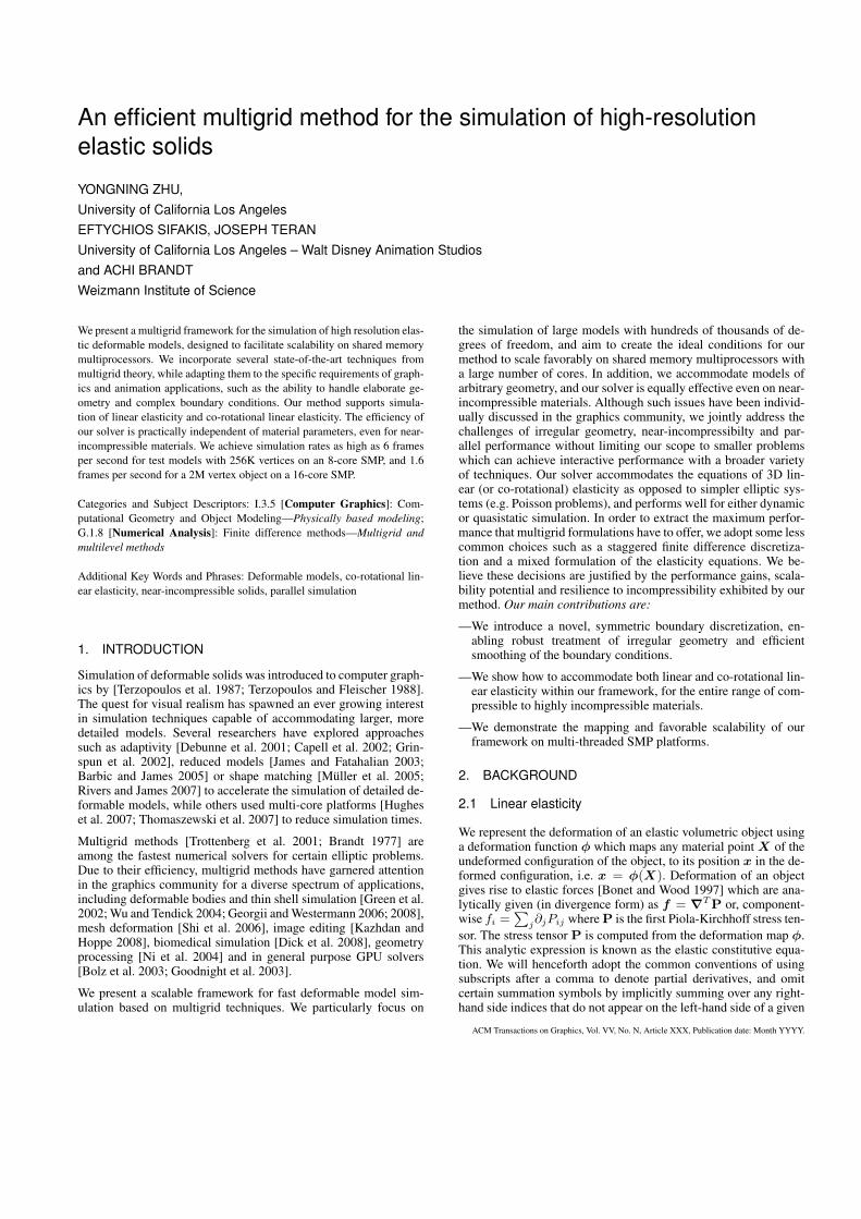
Fig. 1: Staggering of variables in 2D(left) and 3D(right). EquationsL1,L2,L3 are also stored on φ1,φ2,φ3 locations respectively.
Use of staggered variables. In a regular grid it would be mostnatural to specify all components of the vector-valued deformationmap φ at the same locations, for example at the nodes of the grid.However, for equation (3) doing so may result in grid-scale oscilla-tions, especially for near-incompressible materials. This is qualita-tively analogous to an artifact observed in the simulation of fluidswith non-staggered grids, where spurious oscillations may be leftover in the pressure field. For multigrid methods, such oscillatorymodes are problematic, as they may not respect the fundamentalproperty of elliptic PDEs that a low residual implies a smooth error,requiring more elaborate and expensive smoothers to compensate.We avoid this issue by adopting a staggered discretization (Figure1), which is free of this oscillatory behavior. More specifically, φivariables are stored at the centers of grid faces perpendicular to theCartesian axis vector ei. For example, φ1 values are stored on gridfaces perpendicular to e1, i.e. those parallel to the yz-plane. Thesame strategy is followed in 2D, where faces of grid cells are nowidentified with grid edges, thus φ1 values are stored at the center ofy-oriented edges, and φ2 values at the center of x-oriented edges.We define discrete first-order derivatives using central differences:
D1u[x, y, z] = u[x+ 12hx, y, z]− u[x− 1
2hx, y, z]
D2u[x, y, z] = u[x, y+ 12hy, z]− u[x, y− 1
2hy, z]
D3u[x, y, z] = u[x, y, z+ 12hz]− u[x, y, z− 1
2hz]
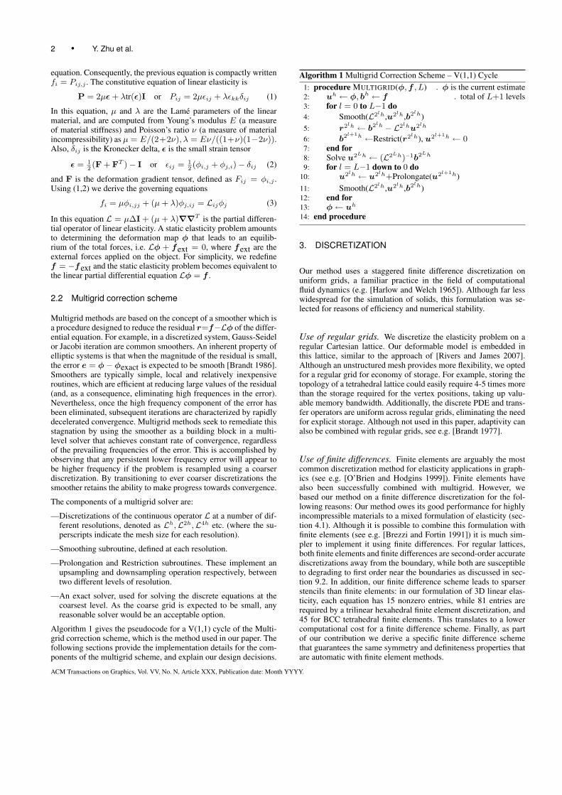
where (hx, hy, hz) are the dimensions of the background grid cells.Second-order derivative stencils are defined as the composition oftwo first-order stencils, i.e. Dij = DiDj . An implication of thesedefinitions is that the discrete first derivative of a certain quantitywill not be collocated with it. For example, all derivatives of theform Diφi are naturally defined at cell centers, while D1φ2 is lo-cated at centers of z-oriented edges in 3D, and at grid nodes in2D. However, derivatives are centered at the appropriate locationsfor a convenient discretization of (3). In particular, all stencils in-volved in the discretization of equation Li are naturally centeredon the location of variable φi. Thus, the staggering of the unknownvariables implies a natural staggering of the discretized differentialequations. Figure 2 illustrates this fact in 2D, where the discretestencils for the operators L1 and L2 from (3) are shown to be natu-rally centered at φ1 and φ2 variable locations, respectively.
4. CONSTRUCTION OF THE SMOOTHING OPERATOR
A majority of elastic materials of interest to computer graphics(e.g. the muscles and flesh of animated characters) are ideallyincompressible. A number of authors [Irving et al. 2007; Kauf-mann et al. 2008] have discussed the simulation challenges of near-incompressible materials and proposed solutions. For a multigrid
Fig. 2: Discrete stencils for operators L1(left) and L2(right) of the PDEsystem (3). The red and green nodes of the stencil correspond to φ1 and φ2
values respectively. The dashed square indicates the center of the stencil,where the equation is evaluated.
solver, naive use of standard smoothers (e.g. Gauss-Seidel) in thepresence of high incompressibility could lead to slow convergenceor even loss of stability. Our proposed solution is computationallyinexpensive and achieves fast convergence independent of materialparameters.
4.1 Augmentation and stable discretization
When the Poisson’s ratio approaches the incompressible limit ν →0.5, the Lame parameter λ becomes several orders of magnitudelarger than µ. As a consequence, the dominant term of the elastic-ity operator L = µ∆I+(µ+λ)∇∇T is the rank deficient operator(µ+λ)∇∇T ; thus L becomes near-singular. More specifically, wesee that any divergence-free field φ will be in the nullspace of thedominant term, i.e. λ∇∇Tφ = 0. Thus, a solution to the elasticityPDE Lφ = f could be perturbed by a divergence-free displace-ment of substantial amplitude, without introducing a large residualfor the differential equation. These perturbations can be arbitrar-ily oscillatory, and lead to high-frequency errors that the multigridmethod cannot smooth efficiently or correct using information froma coarser grid. Fortunately, this complication is not a result of in-herently problematic material behavior, but rather an artifact of theform of the governing equations. Our solution is to reformulate thePDEs of elasticity into an equivalent system, which does not suf-fer from the near-singularity of the original. This stable differentialdescription of near-incompressible elasticity is adapted from thetheory of mixed variational formulations [Brezzi and Fortin 1991].We introduce a new auxiliary variable p (which we call pressure)defined as p = −(λ/µ)∇Tφ = −(λ/µ)divφ. We can write
Lφ = µ(∆I + ∇∇T )φ+ λ∇(∇Tφ)
= µ(∆I + ∇∇T )φ− µ∇p (4)
Thus, the equilibrium equation Lφ = f is equivalently written as(µ(∆I+∇∇T ) −µ∇
µ∇T µ2
λ
)(φp
)=
(f0
)(5)
The top of system (5) follows directly from equation (4), while thebottom is the definition of pressure p. Conversely, the original dif-ferential equation (3) can be obtained from (5) by simply eliminat-ing the pressure variable. Thus the augmented differential equationsystem of (5) is equivalent to the governing equations of linear elas-ticity (e.g. the two systems agree in the value of φ when solved).
ACM Transactions on Graphics, Vol. VV, No. N, Article XXX, Publication date: Month YYYY.
4 • Y. Zhu et al.
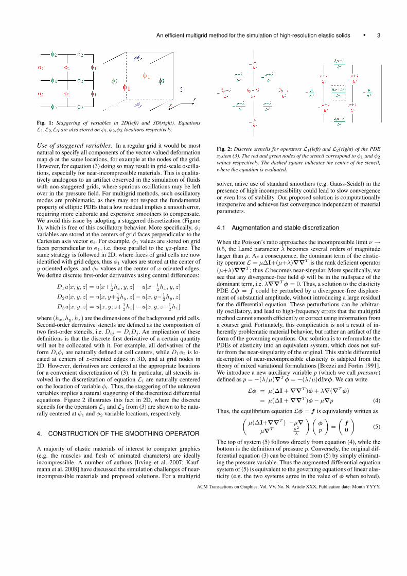
Fig. 3: Placement of pressures in 2D (left) and 3D (right).
The important consequence of this manipulation is that this newdiscretization is stable, in the sense that the system can be smoothedwith standard methods without leaving spurious oscillatory modes.This property can be rigorously proved via Fourier analysis; wecan verify however that as λ tends to infinity, the term µ2/λ van-ishes, and the resulting limit system is now non-singular. In section4.2 we describe a simple smoother, specifically tailored to equation(5). The newly introduced pressure variables are also discretizedon an offset Cartesian lattice, with pressures stored in cell centers(see Figure 3). Pressure equations are also cell centered. As was thecase with the non-augmented elasticity equations, the staggering ofdeformation (φ) and pressure (p) variables is such that all discretedifferential operators are well defined where they are needed.
4.2 Distributive smoothing
The discretization of system (5) yields a symmetric, yet indefinitematrix (discrete first order derivatives are skew-symmetric). Al-though this system has the stability to admit efficient local smooth-ing, this cannot be accomplished with a standard Gauss-Seidel orJacobi iteration. Additionally, for a differential equation such as (5)exhibiting nontrivial coupling between the variables φ1, φ2, φ3 andp, a smoothing scheme which smoothes a given equation by updat-ing several variables at once is often the optimal choice in terms ofefficiency [Trottenberg et al. 2001]. The technique we use in ourformulation is the distributive smoothing approach. This techniquewas applied to the Stokes equation in [Brandt and Dinar 1978]while [Gaspar et al. 2008] discussed its application to linear elastic-ity. In section 7 we generalize it to co-rotated linear elasticity. Letus redefineL to denote the augmented differential operator of equa-tion (5), and write u = (φ, p) for the augmented set of unknownsand b = (f , 0) for the right-hand side vector. Thus, system (5) iswritten as Lu = b. Consider the change of variables(
φp
)=
(I −∇
∇T −2∆
)(ψq
)or u =Mv (6)
where v = (ψ, q) is the vector of auxiliary unknown variables,and M is called the distribution matrix. In accordance with ourstaggered formulation, the components ψ1, ψ2, ψ3 of the auxiliaryvector ψ will be collocated with φ1, φ2, φ3 respectively, while qand p values are also collocated. Using the change of variables ofequation (6), our augmented systemLu = b is equivalently writtenas LMv = b. Composing the operators L andM yields
LM =
(µ∆I 0
µ(1 + µλ
)∇T −µ(1 + 2µλ
)∆
)(7)
That is, the composed system is lower triangular, and its diago-nal elements are simply Laplacian operators. This system can be
smoothed with any scheme that works for the Poisson equation, in-cluding the Gauss-Seidel or Jacobi methods. In fact, the entire sys-tem can be smoothed with the efficiency of the Poisson equation,following a forward substitution approach, i.e. we smooth all ψ1-centered equations across the domain first, followed by sweeps ofψ2, ψ3, and q-centered equations in sequence.While we do not nec-essarily have the auxiliary variables (ψ, q) at our disposal, such anexplicit transformation is not necessary. Consider the Gauss-Seideliteration for the system Lu = b: At every step, we calculate apoint-wise correction to the variable ui, such that the residual ofthe collocated equation Li will vanish. That is, we replace variableui with ui + δ (or u with u+ δei) such that:
eTi (b− L(u+ δei)) = 0⇒ (eTi Lei)δ = eTi (b− Lu)
The last equation is equivalent to Liiδ = roldi or δ = rold
i /Lii,where Lii is the i-th diagonal element of the discrete operator androldi denotes the i-th component of the residual. In an analogous
fashion, a Gauss-Seidel step on the distributed system LMv = bamounts to changing ψi into ψi + δ (or v into v + δei) such thatthe i-th residual of the distributed equation is annihilated
eTi (b− LM(v + δei)) = 0⇒ eTi (b− L(u+ δMei)) = 0
⇒ (eTi LMei)δ = eTi (b− Lu)⇒ δ = roldi /(LM)ii
In this derivation the auxiliary vector v is only used in the formMv which is equal to the value of the original variable u. Thus,after the value of δ has been determined,u is updated tou+δMei.The computational cost of distributive smoothing is comparable tothat of simple Gauss-Seidel iteration, yet it allows efficient smooth-ing of the equations of linear elasticity, independent of Poisson’s ra-tio. We summarize the distributive smoothing process in Algorithm2.
Algorithm 2 Distributive Smoothing1: procedure DISTRIBUTIVESMOOTHING(L,M,u,b)2: for v in {φ1, φ2, φ3, p} do . Must be in this exact order3: for i in Lattice[v] do . i is an equation index4: r ← bi − Li · u . Li is the i-th row of L5: δ ← r/(LM)ii6: u += δmT
i . mi is the i-th row ofM7: end for8: end for9: end procedure
5. TREATMENT OF BOUNDARIES
The previous sections did not address the effect of boundaries, in-stead focusing on the treatment of the interior region. The efficiencyof the interior smoother can be evaluated using a periodic domain.In fact, it is known [Brandt 1994] that a boundary value problemcan be solved at the same efficiency as a periodic problem, at theexpense of more intensive smoothing at the boundary. In theoreti-cal studies, the computational overhead of this additional boundarysmoothing is often overlooked, as the cost of interior smoothing isasymptotically expected to dominate. Nevertheless, practical prob-lem sizes may never reach the asymptotic regime and slow, genericboundary smoothers can pose a performance bottleneck. In thissection, we develop a boundary discretization strategy, includinga novel treatment of traction boundary conditions, that facilitatesthe design of efficient and inexpensive boundary smoothers.
ACM Transactions on Graphics, Vol. VV, No. N, Article XXX, Publication date: Month YYYY.
An efficient multigrid method for the simulation of high-resolution elastic solids • 5
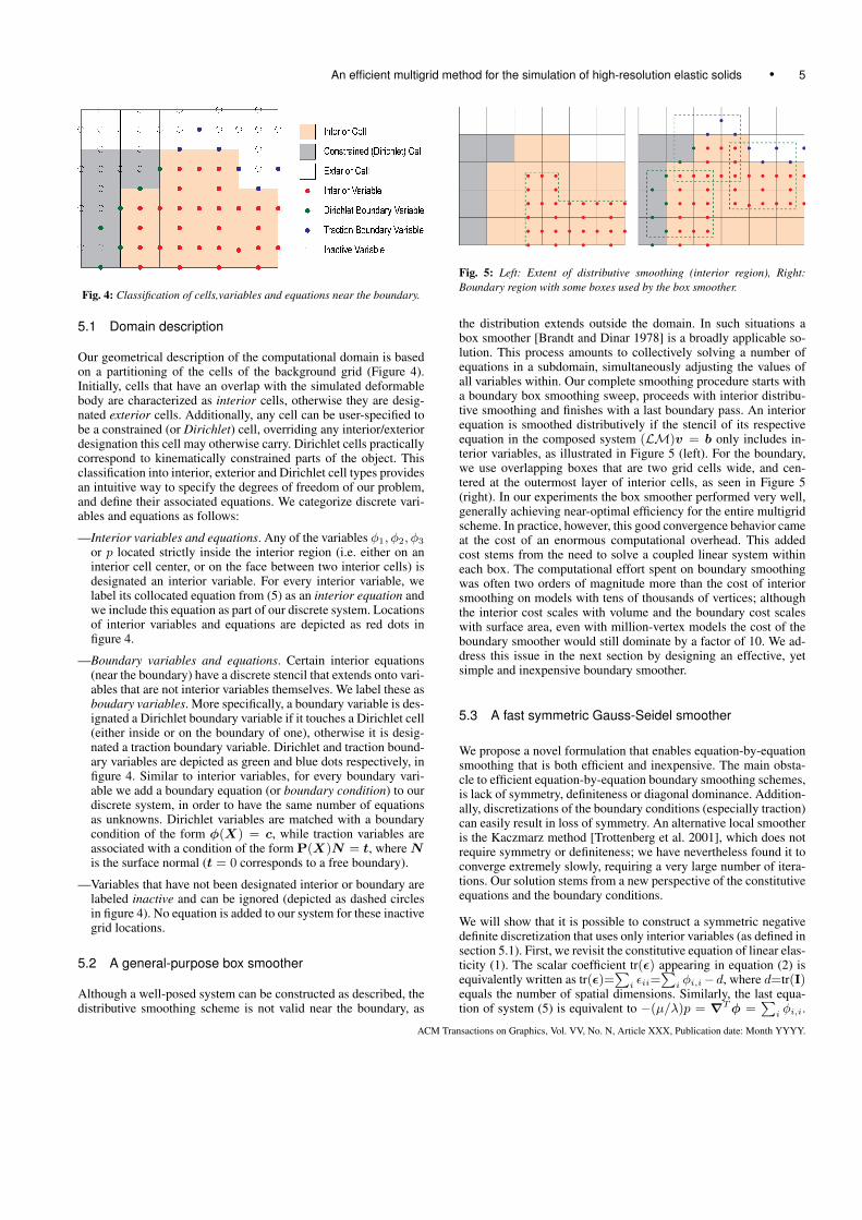
Fig. 4: Classification of cells,variables and equations near the boundary.
5.1 Domain description
Our geometrical description of the computational domain is basedon a partitioning of the cells of the background grid (Figure 4).Initially, cells that have an overlap with the simulated deformablebody are characterized as interior cells, otherwise they are desig-nated exterior cells. Additionally, any cell can be user-specified tobe a constrained (or Dirichlet) cell, overriding any interior/exteriordesignation this cell may otherwise carry. Dirichlet cells practicallycorrespond to kinematically constrained parts of the object. Thisclassification into interior, exterior and Dirichlet cell types providesan intuitive way to specify the degrees of freedom of our problem,and define their associated equations. We categorize discrete vari-ables and equations as follows:
—Interior variables and equations. Any of the variables φ1, φ2, φ3
or p located strictly inside the interior region (i.e. either on aninterior cell center, or on the face between two interior cells) isdesignated an interior variable. For every interior variable, welabel its collocated equation from (5) as an interior equation andwe include this equation as part of our discrete system. Locationsof interior variables and equations are depicted as red dots infigure 4.
—Boundary variables and equations. Certain interior equations(near the boundary) have a discrete stencil that extends onto vari-ables that are not interior variables themselves. We label these asboudary variables. More specifically, a boundary variable is des-ignated a Dirichlet boundary variable if it touches a Dirichlet cell(either inside or on the boundary of one), otherwise it is desig-nated a traction boundary variable. Dirichlet and traction bound-ary variables are depicted as green and blue dots respectively, infigure 4. Similar to interior variables, for every boundary vari-able we add a boundary equation (or boundary condition) to ourdiscrete system, in order to have the same number of equationsas unknowns. Dirichlet variables are matched with a boundarycondition of the form φ(X) = c, while traction variables areassociated with a condition of the form P(X)N = t, whereNis the surface normal (t = 0 corresponds to a free boundary).
—Variables that have not been designated interior or boundary arelabeled inactive and can be ignored (depicted as dashed circlesin figure 4). No equation is added to our system for these inactivegrid locations.
5.2 A general-purpose box smoother
Although a well-posed system can be constructed as described, thedistributive smoothing scheme is not valid near the boundary, as
Fig. 5: Left: Extent of distributive smoothing (interior region), Right:Boundary region with some boxes used by the box smoother.
the distribution extends outside the domain. In such situations abox smoother [Brandt and Dinar 1978] is a broadly applicable so-lution. This process amounts to collectively solving a number ofequations in a subdomain, simultaneously adjusting the values ofall variables within. Our complete smoothing procedure starts witha boundary box smoothing sweep, proceeds with interior distribu-tive smoothing and finishes with a last boundary pass. An interiorequation is smoothed distributively if the stencil of its respectiveequation in the composed system (LM)v = b only includes in-terior variables, as illustrated in Figure 5 (left). For the boundary,we use overlapping boxes that are two grid cells wide, and cen-tered at the outermost layer of interior cells, as seen in Figure 5(right). In our experiments the box smoother performed very well,generally achieving near-optimal efficiency for the entire multigridscheme. In practice, however, this good convergence behavior cameat the cost of an enormous computational overhead. This addedcost stems from the need to solve a coupled linear system withineach box. The computational effort spent on boundary smoothingwas often two orders of magnitude more than the cost of interiorsmoothing on models with tens of thousands of vertices; althoughthe interior cost scales with volume and the boundary cost scaleswith surface area, even with million-vertex models the cost of theboundary smoother would still dominate by a factor of 10. We ad-dress this issue in the next section by designing an effective, yetsimple and inexpensive boundary smoother.
5.3 A fast symmetric Gauss-Seidel smoother
We propose a novel formulation that enables equation-by-equationsmoothing that is both efficient and inexpensive. The main obsta-cle to efficient equation-by-equation boundary smoothing schemes,is lack of symmetry, definiteness or diagonal dominance. Addition-ally, discretizations of the boundary conditions (especially traction)can easily result in loss of symmetry. An alternative local smootheris the Kaczmarz method [Trottenberg et al. 2001], which does notrequire symmetry or definiteness; we have nevertheless found it toconverge extremely slowly, requiring a very large number of itera-tions. Our solution stems from a new perspective of the constitutiveequations and the boundary conditions.
We will show that it is possible to construct a symmetric negativedefinite discretization that uses only interior variables (as defined insection 5.1). First, we revisit the constitutive equation of linear elas-ticity (1). The scalar coefficient tr(ε) appearing in equation (2) isequivalently written as tr(ε)=
∑iεii=
∑iφi,i−d, where d=tr(I)
equals the number of spatial dimensions. Similarly, the last equa-tion of system (5) is equivalent to −(µ/λ)p = ∇Tφ =
∑iφi,i.
ACM Transactions on Graphics, Vol. VV, No. N, Article XXX, Publication date: Month YYYY.
6 • Y. Zhu et al.
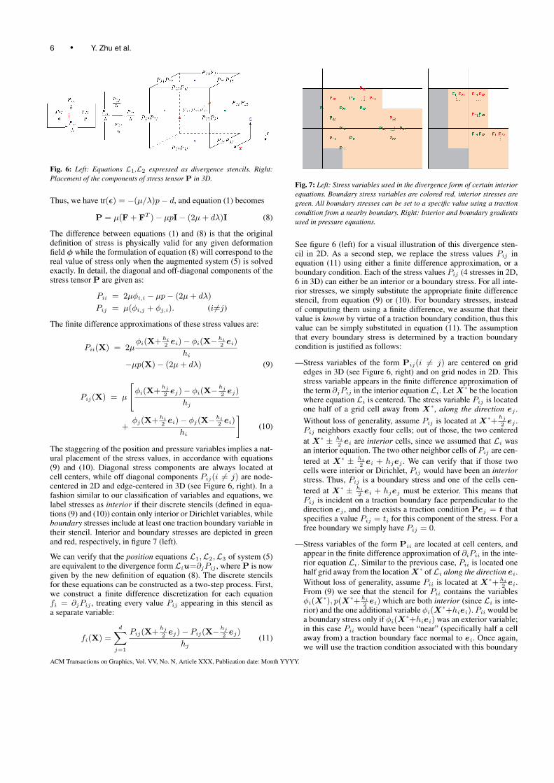
Fig. 6: Left: Equations L1,L2 expressed as divergence stencils. Right:Placement of the components of stress tensor P in 3D.
Thus, we have tr(ε) = −(µ/λ)p− d, and equation (1) becomes
P = µ(F + FT )− µpI− (2µ+ dλ)I (8)
The difference between equations (1) and (8) is that the originaldefinition of stress is physically valid for any given deformationfield φ while the formulation of equation (8) will correspond to thereal value of stress only when the augmented system (5) is solvedexactly. In detail, the diagonal and off-diagonal components of thestress tensor P are given as:
Pii = 2µφi,i − µp− (2µ+ dλ)
Pij = µ(φi,j + φj,i). (i 6=j)
The finite difference approximations of these stress values are:
Pii(X) = 2µφi(X+hi
2ei)− φi(X−hi
2ei)
hi−µp(X)− (2µ+ dλ) (9)
Pij(X) = µ
[φi(X+
hj
2ej)− φi(X−
hj
2ej)
hj
+φj(X+hi
2ei)− φj(X−hi
2ei)
hi
](10)
The staggering of the position and pressure variables implies a nat-ural placement of the stress values, in accordance with equations(9) and (10). Diagonal stress components are always located atcell centers, while off diagonal components Pij(i 6= j) are node-centered in 2D and edge-centered in 3D (see Figure 6, right). In afashion similar to our classification of variables and equations, welabel stresses as interior if their discrete stencils (defined in equa-tions (9) and (10)) contain only interior or Dirichlet variables, whileboundary stresses include at least one traction boundary variable intheir stencil. Interior and boundary stresses are depicted in greenand red, respectively, in figure 7 (left).
We can verify that the position equations L1,L2,L3 of system (5)are equivalent to the divergence form Liu=∂jPij , where P is nowgiven by the new definition of equation (8). The discrete stencilsfor these equations can be constructed as a two-step process. First,we construct a finite difference discretization for each equationfi = ∂jPij , treating every value Pij appearing in this stencil asa separate variable:
fi(X) =
d∑j=1
Pij(X+hj
2ej)− Pij(X−
hj
2ej)
hj(11)
Fig. 7: Left: Stress variables used in the divergence form of certain interiorequations. Boundary stress variables are colored red, interior stresses aregreen. All boundary stresses can be set to a specific value using a tractioncondition from a nearby boundary. Right: Interior and boundary gradientsused in pressure equations.
See figure 6 (left) for a visual illustration of this divergence sten-cil in 2D. As a second step, we replace the stress values Pij inequation (11) using either a finite difference approximation, or aboundary condition. Each of the stress values Pij (4 stresses in 2D,6 in 3D) can either be an interior or a boundary stress. For all inte-rior stresses, we simply substitute the appropriate finite differencestencil, from equation (9) or (10). For boundary stresses, insteadof computing them using a finite difference, we assume that theirvalue is known by virtue of a traction boundary condition, thus thisvalue can be simply substituted in equation (11). The assumptionthat every boundary stress is determined by a traction boundarycondition is justified as follows:
—Stress variables of the form Pij(i 6= j) are centered on gridedges in 3D (see Figure 6, right) and on grid nodes in 2D. Thisstress variable appears in the finite difference approximation ofthe term ∂jPij in the interior equationLi. LetX∗ be the locationwhere equation Li is centered. The stress variable Pij is locatedone half of a grid cell away from X∗, along the direction ej .Without loss of generality, assume Pij is located at X∗+
hj
2ej .
Pij neighbors exactly four cells; out of those, the two centeredat X∗ ± hi
2ei are interior cells, since we assumed that Li was
an interior equation. The two other neighbor cells of Pij are cen-tered at X∗ ± hi
2ei + hjej . We can verify that if those two
cells were interior or Dirichlet, Pij would have been an interiorstress. Thus, Pij is a boundary stress and one of the cells cen-tered at X∗ ± hi
2ei + hjej must be exterior. This means that
Pij is incident on a traction boundary face perpendicular to thedirection ej , and there exists a traction condition Pej = t thatspecifies a value Pij = ti for this component of the stress. For afree boundary we simply have Pij = 0.
—Stress variables of the form Pii are located at cell centers, andappear in the finite difference approximation of ∂iPii in the inte-rior equation Li. Similar to the previous case, Pii is located onehalf grid away from the locationX∗ ofLi along the direction ei.Without loss of generality, assume Pii is located at X∗+hi
2ei.
From (9) we see that the stencil for Pii contains the variablesφi(X
∗), p(X∗+hi2ei) which are both interior (since Li is inte-
rior) and the one additional variable φi(X∗+hiei).Pii would bea boundary stress only if φi(X∗+hiei) was an exterior variable;in this case Pii would have been “near” (specifically half a cellaway from) a traction boundary face normal to ei. Once again,we will use the traction condition associated with this boundary
ACM Transactions on Graphics, Vol. VV, No. N, Article XXX, Publication date: Month YYYY.
An efficient multigrid method for the simulation of high-resolution elastic solids • 7
to set Pii = ti (or Pii = 0 for a free boundary). The subtlety ofthis formulation is that the stress variable Pii is not located ex-actly on the boundary; nevertheless the discrete stencil for Pii isstill a valid first-order approximation of the Pii at the boundary.
In summary, we have justified that all boundary stress variables canbe eliminated (and replaced with known constants) from the diver-gence form of interior position equations. Notably, for equationsthat are far enough from the traction boundary (specifically, thosethat do not require any boundary stresses in equation (8)), this pro-cess yields exactly the same results as the direct discretization ofsystem (5). A similar treatment is performed on the discretizationof the pressure equation Lp=µ
∑iFii + µ2
λp. Similar to stresses,
the deformation gradients Fii are also characterized as interior orboundary, based on whether they touch traction boundary variables.Since Pii = 2µFii−µp−(2λ+dµ), we observe that Fii is bound-ary if and only if the stress Pii is boundary (see figure 7, right). Forsuch boundary gradients or stresses we can use the traction con-dition Pii = ti to eliminate Fii from the pressure equation. Thisis accomplished by replacing Lp ← Lp− 1
2(Pii − ti) for every
boundary gradient Fii.
Our manipulations effectively remove all traction boundary vari-ables from the discretization of the interior equations. For everyDirichlet boundary variable, we assume a Dirichlet condition ofthe form φi = ci is provided. Thus, we can substitute a given valuefor every Dirichlet variable in the stencil of every interior equationthat uses it. As a result, our overall discrete system can be writtenas L∗u∗ = b − bD = b∗, where u∗ only contains interior vari-ables, and bD results from moving the Dirichlet conditions to theright-hand side. The discrete system matrix L∗ has as many rowsand columns as interior variables, and will differ from L near theboundaries, as it incorporates the effect of the boundary conditions.An analysis of our formulation can verify that L∗ has the form
L∗ =
(Lφ GGT Dp
)In this formulation Lφ is symmetric, negative definite, and Dp isa diagonal matrix with positive diagonal elements. As a final step,we define the substitution matrix U
U =
(I −GD−1
p
0 I
)and use it to pre-multiply our equation as
UL∗u∗ =
(Lφ −GD−1
p GT 0GT Dp
)u∗ = Ub∗ (12)
The top left block Lφ −GD−1p GT is essentially a symmetric and
negative definite discretization of our non-augmented system (3)and can be smoothed via Gauss-Seidel iteration. The boundary andinterior regions are smoothed in separate sweeps; during the sweepof the boundary smoother, all interior variables not being smoothedare effectively treated as Dirichlet values. The boundary smootheris confined in a narrow region between boundary conditions (vari-ables of this narrow band are depicted in red in Figure 5, right).This narrow support of the boundary smoother has a strong stabi-lizing effect, and compensates for any difficulties encountered withnear-incompressible materials. In practice, we found that 2 Gauss-Seidel boundary sweeps for every sweep of the distributive interiorsmoother are sufficient for Poisson’s ratio up to ν = .45, while 3-4Gauss-Seidel sweeps suffice for values as high as ν = .495. Fi-nally, we note that Gauss-Seidel is not the only option for smooth-
ing the discrete system derived in this section; in fact it is evenpossible to use a distributive smoother as in Algorithm 2, takingcare to restrict the distribution stencil to active variables.
After completing the smoothing process, we need to update the val-ues of the pressure and traction boundary variables that were pre-viously annihilated. Since the lower right block of equation (12) isdiagonal, all pressure equations can be satisfied exactly via a simpleGauss-Seidel sweep. Similarly, the boundary traction variables canbe updated using the traction conditions Pij = ti in a simple back-substitution step, first updating variables on faces between interiorand exterior cells, and then variables located at half-cell distanceaway from the interior region. Notably, at the end of the process allboundary conditions are satisfied exactly (i.e. they will have zeroresiduals), which simplifies our inter-grid transfers discussed next.
6. CONSTRUCTION OF THE TRANSFER OPERATORS
We designed the Restriction (R) and Prolongation (P) operatorsemployed by algorithm 1 aiming to keep implementation as in-expensive as possible, while conforming to the textbook accuracyrequirements for full multigrid efficiency (see [Trottenberg et al.2001]). We define the following 1D averaging operators
B1u[x] = 12u[x−h
2] + 1
2u[x+h
2]
B2u[x] = 14u[x−h] + 1
2u[x] + 1
4u[x+h]
B3u[x] = 18u[x− 3h
2] + 3
8u[x+h
2] + 3
8u[x−h
2] + 1
8u[x+ 3h
2]
The restriction and prolongation operators will be defined as tensorproduct stencils of the preceding 1D operators as
R1 = B2 ⊗ B1 ⊗ B1 PT1 = 8 B2 ⊗ B3 ⊗ B3
R2 = B1 ⊗ B2 ⊗ B1 PT2 = 8 B3 ⊗ B2 ⊗ B3
R3 = B1 ⊗ B1 ⊗ B2 PT3 = 8 B3 ⊗ B3 ⊗ B2
Rp = B1 ⊗ B1 ⊗ B1 PTp = 8 B1 ⊗ B1 ⊗ B1
where Ri,Pi are the restriction and prolongation operators usedfor variable ui, respectively, and Rp,Pp are the operators used forthe pressure variables. Our restriction and prolongation are not thetranspose of one another (as commonly done in other methods) butthis practice is not unusual or problematic, see e.g. [Brandt 1977].Our domain description for the finest grid was based on a partition-ing of the cells into interior, exterior and Dirichlet. The coarse gridis derived from the natural 8-to-1 coarsening of the Cartesian back-ground lattice. Furthermore, a coarse cell is designated a Dirichletcell if any of its eight fine sub-cells is Dirichlet. If any of the finesub-cells are interior and none is Dirichlet, the coarse cell will beconsidered interior. Otherwise, the coarse cell is exterior. Thus, thecoarse active domain is geometrically a superset of the fine, whileits Dirichlet parts are extended. Despite this geometrical discrep-ancy, which is no larger than the grid cell size, we were still able toobtain a highly efficient multigrid scheme as described next.
In our treatment of boundary conditions in section 5.3 we effec-tively forced all boundary conditions to be satisfied exactly afterevery application of the smoother. In general, if a smoother leavesa residual on the boundary conditions, this residual has to be re-stricted. In our case all boundary residuals in the fine grid arezero, thus all coarse boundary conditions will be homogeneous;for Dirichlet equations they will have the form u2h
i = 0 (i.e. thecoarse grid incurs no correction), while traction equations will beof the form P 2h
ij = 0, where P = µ(F + FT ) − µpI is the ho-mogeneous part of P. We also note that, due to the possible ge-
ACM Transactions on Graphics, Vol. VV, No. N, Article XXX, Publication date: Month YYYY.
8 • Y. Zhu et al.
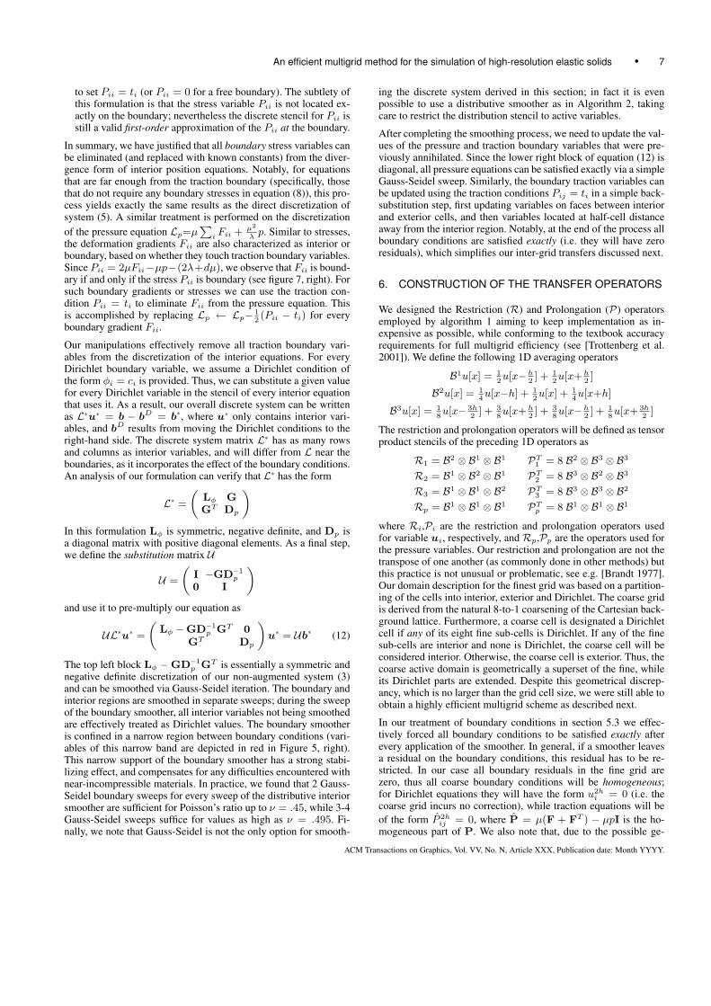
Fig. 8: Boundary discrepancies in the fine (left) and coarse (right) domains.On the right, red dots indicate locations containing Dirichlet conditions onthe coarse grid, but interior equations on the fine grid. On the left, red dotsindicate interior equations that would restrict residuals on one or more lo-cations occupied by Dirichlet conditions on the coarse grid; those restrictedresiduals will be replaced with zero. Green circles indicate fine interiorvariables that prolongate their correction from boundary coarse variables.
ometrical change of the Dirichlet region, certain coarse Dirichletequations will be centered on locations that were interior in the finegrid (shown as red dots in Figure 8, right). The fine grid interiorequations (red dots in Figure 8, left) that would restrict their resid-uals onto these (now Dirichlet) coarse locations, will not have theirresiduals well represented on the coarse grid. We compensate forthis inaccuracy by performing an extra 2-3 sweeps of our boundaryGauss-Seidel smoother over these equations, driving their resid-uals very close to zero, just prior to restriction. A similar inac-curacy may affect the prolongation of the correction: as we pre-viously mentioned, the active region may have extended more inthe coarse grid, compared to the fine. This discrepancy may intro-duce inaccuracies in the coarse grid solution near such relocatedboundaries. Again, we compensate by performing an additional 2-3 Gauss-Seidel smoother sweeps on the locations of the fine gridthat prolongate corrections from such relocated boundary variables(depicted as green circles in Figure 8, left). This simple treatmentproved quite effective to guarantee a good coarse correction despitethe small geometrical discrepancies of the two domains.
7. CO-ROTATIONAL LINEAR ELASTICITY
In the large deformation regime, and in the presence of large ro-tational deformations, the linear elasticity model develops artifactssuch as volumetric distortions in parts of the domain with largerotations. We provide an extension to the co-rotational linear elas-ticity model, which has been used in slightly different forms by anumber of authors in computer graphics [Muller et al. 2002; Hauthand Strasser 2004; Muller and Gross 2004], and has also used withfinite elements and multigrid by [Georgii and Westermann 2006;2008]. The co-rotational formulation extracts the rotational com-ponent of the local deformation at a specific part of the domainby computing the polar decomposition of the deformation gradi-ent tensor F = RS into the rotation R and the symmetric tensorS. The stress is then computed as P = RPL(S), where PL de-notes the stress of a linear material, as described in equation (1).Thus, the co-rotational formulation computes stresses by applyingthe constitutive equation of linear elasticity in a frame of referencethat is rotated with the material deformation as follows:
P = RPL(S) = R[2µ(RTF−I) + λtr(RTF−I)I
]
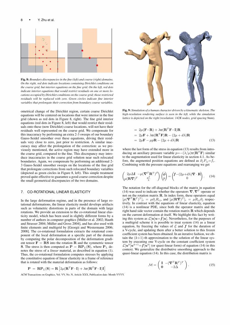
Fig. 9: Simulation of a human character driven by a kinematic skeleton. Thehigh-resolution rendering surface is seen in the left, while the simulationlattice is depicted on the right (resolution: 142K nodes, grid spacing 9mm).
= 2µ(F−R) + λtr(RTF−I)R
= 2µF + λtr(RTF)R− (2µ+ dλ)R
= 2µF− µpR− (2µ+ dλ)R (13)
where the last form of the stress in equation (13) results from intro-ducing an auxiliary pressure variable p=−(λ/µ)tr(RTF) similarto the augmentation used for linear elasticity in section 4.1. As be-fore, the augmented position equations are defined as ∂jPij=fi.Combining with the pressure equations and rearranging we get(
2µ∆I −µ(∇TRT )T
µ(R∇)T µ2
λ
)(φp
)=
(f−(2µ+dλ)∇ ·R
0
). (14)
The notation for the off-diagonal blocks of the matrix in equation(14) was used to indicate whether the operators ∇,∇T operate ornot on the rotation matrix R. In index form, these operators equal[µ(∇TRT )T ]i = µ∂jRij , and [µ(R∇)T ]i = µRij∂j respec-tively. In contrast with the equations of linear elasticity, equation(14) is a nonlinear PDE, since both the operator matrix and theright hand side vector contain the rotation matrix R which dependson the current deformation φ itself. We highlight this fact by writ-ing this system as L[u]u=f [u]. Nevertheless, for the purposes ofa multigrid scheme it is possible to treat system (14) as a linearequation, by freezing the values of L and f for the duration ofa V-cycle, and updating them after a better solution to this frozencoefficient system has been obtained. In an iterative fashion, we ob-tain the (k+1)-th approximation to the solution of the linear sys-tem by executing one V-cycle on the constant coefficient systemL[uk]uk+1=f [uk] (or quasi-linear form) of equation (14) in thiscontext. We generalize the distributive smoothing approach to thequasi-linear equation (14). In this case, the distribution matrix is
M =
(I −(∇TRT )T
0 −2∆
). (15)
ACM Transactions on Graphics, Vol. VV, No. N, Article XXX, Publication date: Month YYYY.
An efficient multigrid method for the simulation of high-resolution elastic solids • 9
Then, the distributed operator LM becomes
LM =
(2µ∆I 2µ
[(∇TRT )T∆−∆(∇TRT )T
]µ(R∇)T −µ(1 + 2µ
λ)∆
)(16)
The top right block of LM would be equal to zero if R is a spa-tially constant rotation, but not in the general case. However, neara solution where the rotations are expected to be smooth, this valueis effectively zero, and LM becomes a triangular matrix, simi-lar to the linear case. Effectively, even if the distributed system isnear-triangular, a Gauss-Seidel algorithm will still be an acceptablesmoother. In practice we found distributive Gauss-Seidel to be agood smoother for the quasi-linear problem at all times, althoughthe convergence rates were slightly lower away from the solution.
For the purposes of boundary smoothing, we again derive a sym-metric definite discretization where Gauss-Seidel can be used. Theequations are written in the divergence form Liu=∂jPij and anyexterior stresses are eliminated from the divergence stencil us-ing an appropriate traction equation, as in section 5.3. The onlycomplication is due to the fact that pressures are now multipliedby the non-diagonal matrix R in the augmented stress definition(13), thus off diagonal stresses Pij (i 6= j) require an edge cen-tered pressure value. Since all exterior stresses have been removed,the four incident cells to the edge in question are interior. Thus,we compute the needed pressure value by averaging these fourneighboring pressures. Finally, pressure equations are written asµRijφi,j + (µ2/λ)p = 0, indicating that all gradient values φi,jare needed at a cell center. The stencil for off-diagonal gradientswill be averaged from the four neighboring edge centers, wherethey are naturally defined. If any such gradient is external, we eval-uate this term as RijFij as a frozen coefficient and move it to theright hand side. The resulting discrete system of equations is sym-metric and definite (after substitution of the pressures) and can besmoothed with a Gauss-Seidel procedure as in section 5.3.
8. DYNAMICS
The static formulation of elasticity disregards any dynamic effects.Our method, however, can easily accommodate the simulation ofdynamic deformation; the effect of inertia actually improves theconditioning of the discrete equations. For example, a backwardEuler implicit scheme updates positions as(
I− ∆t
m(∆t+ γ)L
)xn+1 = xn + ∆tvn − γ∆t
mLxn.
Here, γ is the damping coefficient. Velocities are updated asvn+1=(xn+1−xn)/∆t. Up to scaling, this is equivalent to solv-ing the problem Lu−cφ = b. This system can also be augmented,by adding the term−cI to the position equations of (5). Distributivesmoothing can be followed as before, where the bottom right term−2∆ in the distribution matrix is now replaced by−2∆+c/µ. Allother formulations hold unchanged and convergence for this systemwill be at least as good as the static case.
9. RESULTS AND EVALUATION
9.1 Evaluation of solver performance
We first compare the performance of our method with a ConjugateGradients (CG) solver, as illustrated in Figure 11. The left figureplots the reduction of the residual for our synthetic test model: a
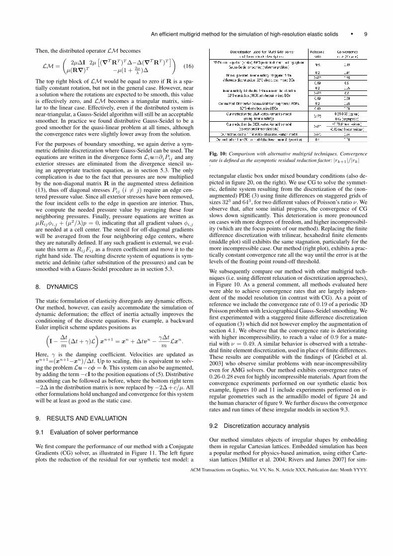
Fig. 10: Comparison with alternative multigrid techniques. Convergencerate is defined as the asymptotic residual reduction factor: |rk+1|/|rk|.
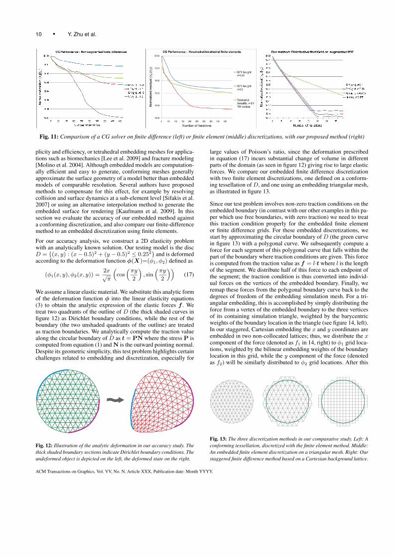
rectangular elastic box under mixed boundary conditions (also de-picted in figure 20, on the right). We use CG to solve the symmet-ric, definite system resulting from the discretization of the (non-augmented) PDE (3) using finite differences on staggered grids ofsizes 323 and 643, for two different values of Poisson’s ratio ν. Weobserve that, after some initial progress, the convergence of CGslows down significantly. This deterioration is more pronouncedon cases with more degrees of freedom, and higher incompressibil-ity (which are the focus points of our method). Replacing the finitedifference discretization with trilinear, hexahedral finite elements(middle plot) still exhibits the same stagnation, particularly for themore incompressible case. Our method (right plot), exhibits a prac-tically constant convergence rate all the way until the error is at thelevels of the floating point round-off threshold.
We subsequently compare our method with other multigrid tech-niques (i.e. using different relaxation or discretization approaches),in Figure 10. As a general comment, all methods evaluated herewere able to achieve convergence rates that are largely indepen-dent of the model resolution (in contrast with CG). As a point ofreference we include the convergence rate of 0.19 of a periodic 3DPoisson problem with lexicographical Gauss-Seidel smoothing. Wefirst experimented with a staggered finite difference discretizationof equation (3) which did not however employ the augmentation ofsection 4.1. We observe that the convergence rate is deterioratingwith higher incompressibility, to reach a value of 0.9 for a mate-rial with ν = 0.49. A similar behavior is observed with a tetrahe-dral finite element discretization, used in place of finite differences.These results are compatible with the findings of [Griebel et al.2003] who observe similar problems with near-incompressibilityeven for AMG solvers. Our method exhibits convergence rates of0.26-0.28 even for highly incompressible materials. Apart from theconvergence experiments performed on our synthetic elastic boxexample, figures 10 and 11 include experiments performed on ir-regular geometries such as the armadillo model of figure 24 andthe human character of figure 9. We further discuss the convergencerates and run times of these irregular models in section 9.3.
9.2 Discretization accuracy analysis
Our method simulates objects of irregular shapes by embeddingthem in regular Cartesian lattices. Embedded simulation has beena popular method for physics-based animation, using either Carte-sian lattices [Muller et al. 2004; Rivers and James 2007] for sim-
ACM Transactions on Graphics, Vol. VV, No. N, Article XXX, Publication date: Month YYYY.
10 • Y. Zhu et al.
Fig. 11: Comparison of a CG solver on finite difference (left) or finite element (middle) discretizations, with our proposed method (right)
plicity and efficiency, or tetrahedral embedding meshes for applica-tions such as biomechanics [Lee et al. 2009] and fracture modeling[Molino et al. 2004]. Although embedded models are computation-ally efficient and easy to generate, conforming meshes generallyapproximate the surface geometry of a model better than embeddedmodels of comparable resolution. Several authors have proposedmethods to compensate for this effect, for example by resolvingcollision and surface dynamics at a sub-element level [Sifakis et al.2007] or using an alternative interpolation method to generate theembedded surface for rendering [Kaufmann et al. 2009]. In thissection we evaluate the accuracy of our embedded method againsta conforming discretization, and also compare our finite-differencemethod to an embedded discretization using finite elements.
For our accuracy analysis, we construct a 2D elasticity problemwith an analytically known solution. Our testing model is the discD = {(x, y) : (x− 0.5)2 + (y − 0.5)2 ≤ 0.252} and is deformedaccording to the deformation function φ(X)=(φ1, φ2) defined as
(φ1(x, y), φ2(x, y)) =2x√π
(cos(πy
2
), sin
(πy
2
))(17)
We assume a linear elastic material. We substitute this analytic formof the deformation function φ into the linear elasticity equations(3) to obtain the analytic expression of the elastic forces f . Wetreat two quadrants of the outline of D (the thick shaded curves infigure 12) as Dirichlet boundary conditions, while the rest of theboundary (the two unshaded quadrants of the outline) are treatedas traction boundaries. We analytically compute the traction valuealong the circular boundary of D as t = PN where the stress P iscomputed from equation (1) and N is the outward pointing normal.Despite its geometric simplicity, this test problem highlights certainchallenges related to embedding and discretization, especially for
Fig. 12: Illustration of the analytic deformation in our accuracy study. Thethick shaded boundary sections indicate Dirichlet boundary conditions. Theundeformed object is depicted on the left, the deformed state on the right.
large values of Poisson’s ratio, since the deformation prescribedin equation (17) incurs substantial change of volume in differentparts of the domain (as seen in figure 12) giving rise to large elasticforces. We compare our embedded finite difference discretizationwith two finite element discretizations, one defined on a conform-ing tessellation ofD, and one using an embedding triangular mesh,as illustrated in figure 13.
Since our test problem involves non-zero traction conditions on theembedded boundary (in contrast with our other examples in this pa-per which use free boundaries, with zero traction) we need to treatthis traction condition properly for the embedded finite elementor finite difference grids. For these embedded discretizations, westart by approximating the circular boundary of D (the green curvein figure 13) with a polygonal curve. We subsequently compute aforce for each segment of this polygonal curve that falls within thepart of the boundary where traction conditions are given. This forceis computed from the traction value as f = l·t where l is the lengthof the segment. We distribute half of this force to each endpoint ofthe segment; the traction condition is thus converted into individ-ual forces on the vertices of the embedded boundary. Finally, weremap these forces from the polygonal boundary curve back to thedegrees of freedom of the embedding simulation mesh. For a tri-angular embedding, this is accomplished by simply distributing theforce from a vertex of the embedded boundary to the three verticesof its containing simulation triangle, weighted by the barycentricweights of the boundary location in the triangle (see figure 14, left).In our staggered, Cartesian embedding the x and y coordinates areembedded in two non-collocated lattices; thus, we distribute the xcomponent of the force (denoted as f1 in 14, right) to φ1 grid loca-tions, weighted by the bilinear embedding weights of the boundarylocation in this grid, while the y component of the force (denotedas f2) will be similarly distributed to φ2 grid locations. After this
Fig. 13: The three discretization methods in our comparative study. Left: Aconforming tessellation, discretized with the finite element method. Middle:An embedded finite element discretization on a triangular mesh. Right: Ourstaggered finite difference method based on a Cartesian background lattice.
ACM Transactions on Graphics, Vol. VV, No. N, Article XXX, Publication date: Month YYYY.
An efficient multigrid method for the simulation of high-resolution elastic solids • 11
Fig. 14: Left: Boundary traction forces are barycentrically distributed tothe vertices of a triangular embedding mesh. Right: In our staggered dis-cretization, each component of the traction force is bilinearly distributed tothe grid locations of the respective (staggered) variable.
remapping, traction forces that have been mapped to locations ofinterior variables are scaled by 1/h2 (to remove the area weightingand convert them to force densities, as in the PDE form of elastic-ity) and then added to the right hand side of the discrete equationLφ = f , while forces mapped to boundary variable locations areconverted back into traction conditions on the faces of the embed-ding grid as ti = fi(N · N ′)/h, where N is the normal to theembedded boundary and N ′ is the normal to boundary face of theembedding grid. Notably, for free (zero-traction) boundaries, thistreatment simply reduces to the method described in section 5.3.
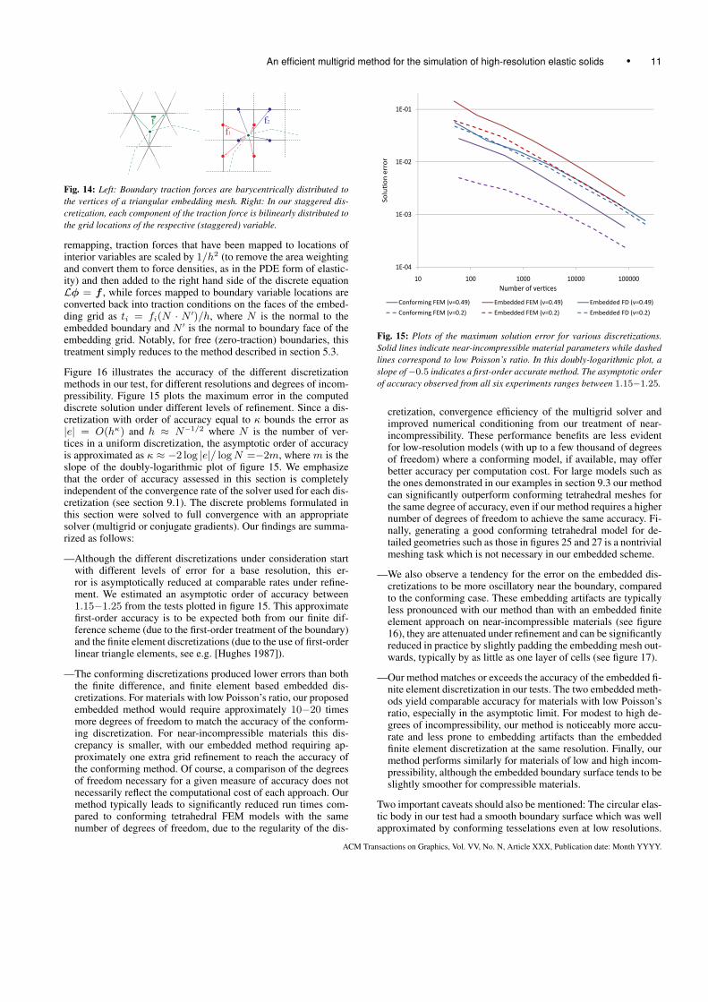
Figure 16 illustrates the accuracy of the different discretizationmethods in our test, for different resolutions and degrees of incom-pressibility. Figure 15 plots the maximum error in the computeddiscrete solution under different levels of refinement. Since a dis-cretization with order of accuracy equal to κ bounds the error as|e| = O(hκ) and h ≈ N−1/2 where N is the number of ver-tices in a uniform discretization, the asymptotic order of accuracyis approximated as κ ≈ −2 log |e|/ logN =−2m, where m is theslope of the doubly-logarithmic plot of figure 15. We emphasizethat the order of accuracy assessed in this section is completelyindependent of the convergence rate of the solver used for each dis-cretization (see section 9.1). The discrete problems formulated inthis section were solved to full convergence with an appropriatesolver (multigrid or conjugate gradients). Our findings are summa-rized as follows:
—Although the different discretizations under consideration startwith different levels of error for a base resolution, this er-ror is asymptotically reduced at comparable rates under refine-ment. We estimated an asymptotic order of accuracy between1.15−1.25 from the tests plotted in figure 15. This approximatefirst-order accuracy is to be expected both from our finite dif-ference scheme (due to the first-order treatment of the boundary)and the finite element discretizations (due to the use of first-orderlinear triangle elements, see e.g. [Hughes 1987]).
—The conforming discretizations produced lower errors than boththe finite difference, and finite element based embedded dis-cretizations. For materials with low Poisson’s ratio, our proposedembedded method would require approximately 10−20 timesmore degrees of freedom to match the accuracy of the conform-ing discretization. For near-incompressible materials this dis-crepancy is smaller, with our embedded method requiring ap-proximately one extra grid refinement to reach the accuracy ofthe conforming method. Of course, a comparison of the degreesof freedom necessary for a given measure of accuracy does notnecessarily reflect the computational cost of each approach. Ourmethod typically leads to significantly reduced run times com-pared to conforming tetrahedral FEM models with the samenumber of degrees of freedom, due to the regularity of the dis-
1E-03
1E-02
1E-01
Solution
err
or
1E-04
10 100 1000 10000 100000Number of vertices
Conforming FEM (ν=0.49) Embedded FEM (ν=0.49) Embedded FD (ν=0.49)
Conforming FEM (ν=0.2) Embedded FEM (ν=0.2) Embedded FD (ν=0.2)
Fig. 15: Plots of the maximum solution error for various discretizations.Solid lines indicate near-incompressible material parameters while dashedlines correspond to low Poisson’s ratio. In this doubly-logarithmic plot, aslope of−0.5 indicates a first-order accurate method. The asymptotic orderof accuracy observed from all six experiments ranges between 1.15−1.25.
cretization, convergence efficiency of the multigrid solver andimproved numerical conditioning from our treatment of near-incompressibility. These performance benefits are less evidentfor low-resolution models (with up to a few thousand of degreesof freedom) where a conforming model, if available, may offerbetter accuracy per computation cost. For large models such asthe ones demonstrated in our examples in section 9.3 our methodcan significantly outperform conforming tetrahedral meshes forthe same degree of accuracy, even if our method requires a highernumber of degrees of freedom to achieve the same accuracy. Fi-nally, generating a good conforming tetrahedral model for de-tailed geometries such as those in figures 25 and 27 is a nontrivialmeshing task which is not necessary in our embedded scheme.
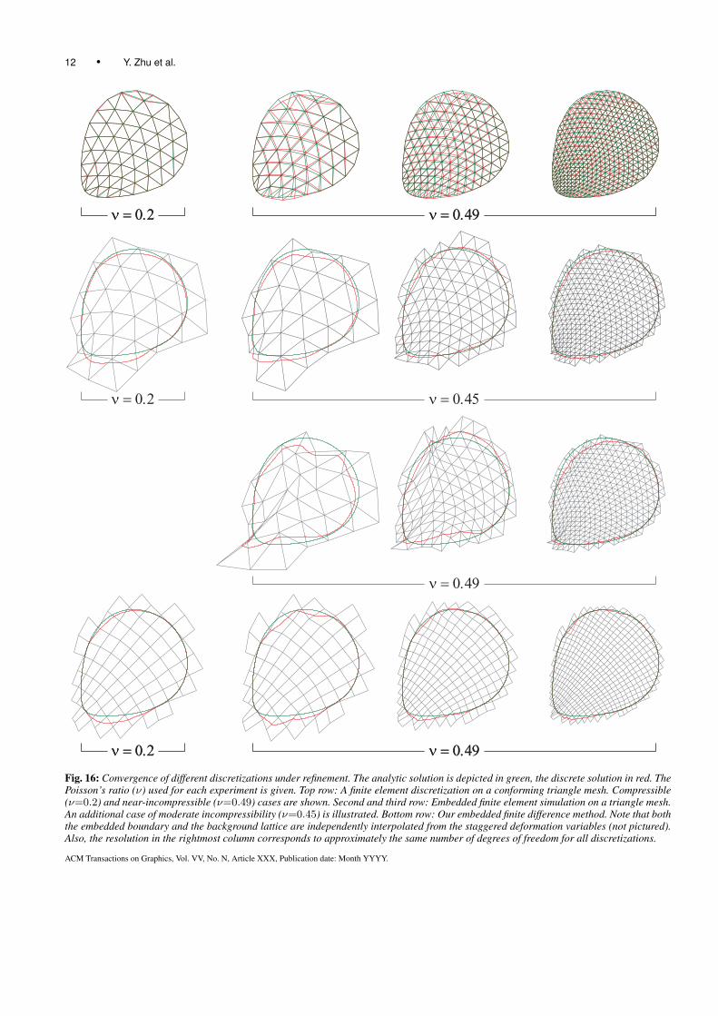
—We also observe a tendency for the error on the embedded dis-cretizations to be more oscillatory near the boundary, comparedto the conforming case. These embedding artifacts are typicallyless pronounced with our method than with an embedded finiteelement approach on near-incompressible materials (see figure16), they are attenuated under refinement and can be significantlyreduced in practice by slightly padding the embedding mesh out-wards, typically by as little as one layer of cells (see figure 17).
—Our method matches or exceeds the accuracy of the embedded fi-nite element discretization in our tests. The two embedded meth-ods yield comparable accuracy for materials with low Poisson’sratio, especially in the asymptotic limit. For modest to high de-grees of incompressibility, our method is noticeably more accu-rate and less prone to embedding artifacts than the embeddedfinite element discretization at the same resolution. Finally, ourmethod performs similarly for materials of low and high incom-pressibility, although the embedded boundary surface tends to beslightly smoother for compressible materials.
Two important caveats should also be mentioned: The circular elas-tic body in our test had a smooth boundary surface which was wellapproximated by conforming tesselations even at low resolutions.
ACM Transactions on Graphics, Vol. VV, No. N, Article XXX, Publication date: Month YYYY.
12 • Y. Zhu et al.
ν = 0.49ν = 0.2
ν = 0.45ν = 0.2
ν = 0.49ν = 0.2
ν = 0.49ν = 0.2 ν = 0.49ν = 0.2
ν = 0.49
Fig. 16: Convergence of different discretizations under refinement. The analytic solution is depicted in green, the discrete solution in red. ThePoisson’s ratio (ν) used for each experiment is given. Top row: A finite element discretization on a conforming triangle mesh. Compressible(ν=0.2) and near-incompressible (ν=0.49) cases are shown. Second and third row: Embedded finite element simulation on a triangle mesh.An additional case of moderate incompressibility (ν=0.45) is illustrated. Bottom row: Our embedded finite difference method. Note that boththe embedded boundary and the background lattice are independently interpolated from the staggered deformation variables (not pictured).Also, the resolution in the rightmost column corresponds to approximately the same number of degrees of freedom for all discretizations.
ACM Transactions on Graphics, Vol. VV, No. N, Article XXX, Publication date: Month YYYY.
An efficient multigrid method for the simulation of high-resolution elastic solids • 13
Highly detailed models with intricate features (see e.g., figures 25and 27) would incur significantly higher approximation errors for aconforming tesselation that does not descend to the resolution levelnecessary to resolve all the geometric detail. Secondly, in our em-bedded examples we used the analytic expression of the deforma-tion field in equation (17) to specify Dirichlet boundary conditionsdirectly on the vertices of the embedding meshes. This can be anacceptable practice for applications such as skeleton-driven charac-ters, where kinematic constraints have a volumetric extent and cantherefore be sampled at the locations of the simulation degrees offreedom. However, when Dirichlet conditions need to be specifiedat sub-grid locations and extrapolating these constraints to simu-lation vertices is not convenient, conforming meshes that resolvethe constraint surface would be at an advantage. In future work wewill investigate adding embedded soft-constraints in our framework(see e.g. [Sifakis et al. 2007]) to provide this additional flexibility.Finally, in our tests we considered discretizations of approximatelyuniform density (even when the mesh topology was irregular). It isalso possible to use an adaptive discretization, either in the form ofan adaptive conforming tesselation or an adaptive finite differencescheme (see e.g. [Losasso et al. 2004]). In fact, there are well estab-lished multigrid methods that operate in conjunction with adaptivediscretizations [Brandt 1977], and we believe the elasticity solverproposed in this paper can be similarly applied to adaptive (e.g. oc-tree) discretizations. We defer this extension to future work, alongwith a principed comparative evaluation of different adaptive dis-cretization schemes for elasticity, especially in light of the nontriv-ial implications adaptivity may have on accuracy, numerical condi-tioning and potential for parallelization.
9.3 Animation tests
In addition to our comparative benchmarks, we tested our methodon models with elaborate, irregular geometries. Figure 9 demon-strates the simulation of flesh of a human character with keyframedskeleton motion. The model was simulated at 2 resolutions yield-ing V-cycle times of 0.62sec for a 142K vertex model (pictured infigure 9), and 3.48sec for a larger resolution with 1.15M vertices(figure 17, right). The convergence rate for this example, as seen inFigures 11(right) and 10, was slightly better than our synthetic boxexamples at 0.24. We attribute this result to the extensive Dirich-let regions throughout the body induced by the kinematic skeleton,which stabilize the model and allow for highly efficient smooth-ing. In contrast, the armadillo model of figure 24 is very weaklyconstrained, with Dirichlet regions defined only over the hands andfeet (see also [Griebel et al. 2003] for a discussion of sub-optimalsmoothing performance with dominating traction boundaries). Inthis model with extensive zero-traction boundary conditions, ourmethod exhibited convergence rates between 0.21-0.35 for the first7-8 V-cycles after a large perturbation; at that point the residualhad been reduced by four orders of magnitude and the model hadvisually reached convergence after just the first few iterations. Sub-sequent V-cycles would ultimately settle at an asymptotic rate of0.62 which could be improved by increasing the intensity of theboundary smoother, although this was not pursued since the modelwas already well converged and the extra smoothing cost wouldnot be practically justified. With typical incremental motion of theboundary conditions, 1-2 V-cycles per frame would be enough toproduce a visually converged animation.
Figure 10 also reports the convergence rates for the armadillomodel of figure 24 simulated using co-rotational linear elasticity.Since the coefficients of the discrete system vary with the current
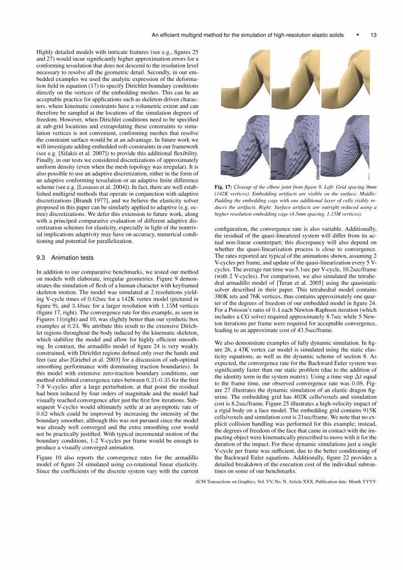
Fig. 17: Closeup of the elbow joint from figure 9. Left: Grid spacing 9mm(142K vertices). Embedding artifacts are visible on the surface. Middle:Padding the embedding cage with one additional layer of cells visibly re-duces the artifacts. Right: Surface artifacts are outright reduced using ahigher resolution embedding cage (4.5mm spacing, 1.15M vertices).
configuration, the convergence rate is also variable. Additionally,the residual of the quasi-linearized system will differ from its ac-tual non-linear counterpart; this discrepancy will also depend onwhether the quasi-linearization process is close to convergence.The rates reported are typical of the animations shown, assuming 2V-cycles per frame, and update of the quasi-linearization every 5 V-cycles. The average run time was 5.1sec per V-cycle, 10.2sec/frame(with 2 V-cycles). For comparison, we also simulated the tetrahe-dral armadillo model of [Teran et al. 2005] using the quasistaticsolver described in their paper. This tetrahedral model contains380K tets and 76K vertices, thus contains approximately one quar-ter of the degrees of freedom of our embedded model in figure 24.For a Poisson’s ratio of 0.4 each Newton-Raphson iteration (whichincludes a CG solve) required approximately 8.7sec while 5 New-ton iterations per frame were required for acceptable convergence,leading to an approximate cost of 43.5sec/frame.
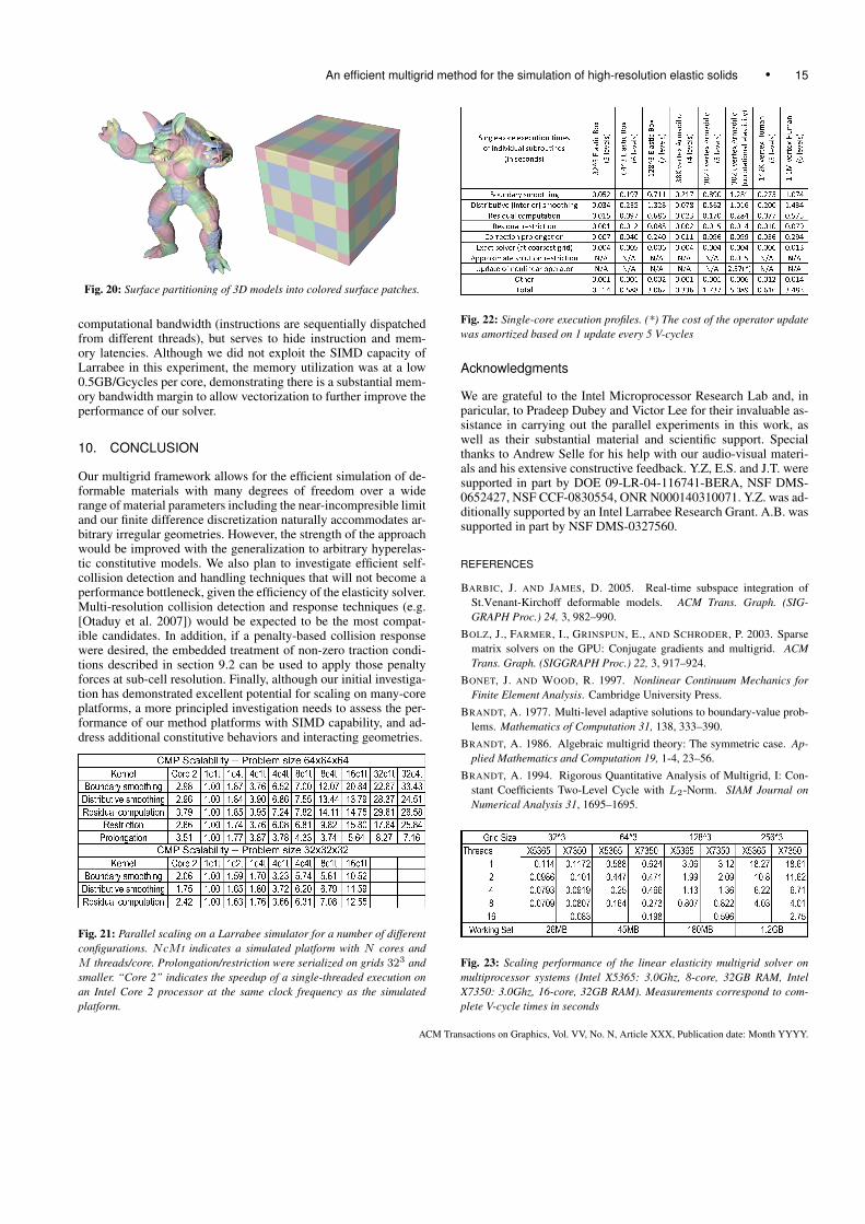
We also demonstrate examples of fully dynamic simulation. In fig-ure 26, a 43K vertex car model is simulated using the static elas-ticity equations, as well as the dynamic scheme of section 8. Asexpected, the convergence rate for the Backward Euler system wassignificantly faster than our static problem (due to the addition ofthe identity term in the system matrix). Using a time step ∆t equalto the frame time, our observed convergence rate was 0.08. Fig-ure 27 illustrates the dynamic simulation of an elastic dragon fig-urine. The embedding grid has 402K cells/voxels and simulationcost is 8.2sec/frame. Figure 25 illustrates a high-velocity impact ofa rigid body on a face model. The embedding grid contains 915Kcells/voxels and simulation cost is 21sec/frame. We note that no ex-plicit collision handling was performed for this example; instead,the degrees of freedom of the face that came in contact with the im-pacting object were kinematically prescribed to move with it for theduration of the impact. For these dynamic simulations just a singleV-cycle per frame was sufficient, due to the better conditioning ofthe Backward Euler equations. Additionally, figure 22 provides adetailed breakdown of the execution cost of the individual subrou-tines on some of our benchmarks.
ACM Transactions on Graphics, Vol. VV, No. N, Article XXX, Publication date: Month YYYY.
14 • Y. Zhu et al.
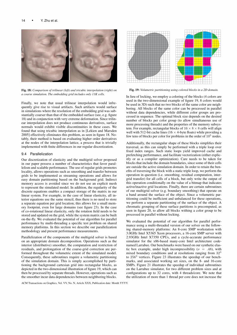
Fig. 18: Comparison of trilinear (left) and tricubic interpolation (right) ona coarse simulation. The embedding grid includes only 11K cells.
Finally, we note that usual trilinear interpolation would infre-quently give rise to visual artifacts. Such artifacts would surfacein simulations where the resolution of the embedding grid was sub-stantially coarser than that of the embedded surface (see, e.g. figure18) and in conjunction with very extreme deformation. Since trilin-ear interpolation does not produce continuous derivatives, surfacenormals would exhibit visible discontinuities in these cases. Wefound that using tricubic interpolation as in [Lekien and Marsden2005] effectively eliminates this problem, as seen in figure 18. No-tably, their method is based on evaluating higher order derivativesat the nodes of the interpolation lattice, a process that is triviallyimplemented with finite differences in our regular discretization.
9.4 ParallelizationOur discretization of elasticity and the multigrid solver proposedin our paper possess a number of characteristics that favor paral-lelism and scalable performance. The use of regular grids promoteslocality, allows operations such as smoothing and transfer betweengrids to be implemented as streaming operations and allows foreasy domain partitioning based on the background grid. Indirectmemory access is avoided since we do not use an explicit meshto represent the simulated model. In addition, the regularity of thediscrete equations enables a compact storage of the matrix in ourlinear system. For example, in the case of linear elasticity, all in-terior equations use the same stencil, thus there is no need to storea separate equation per grid location; this allows for a small mem-ory footprint, even for large domains (see figure 23). In the caseof co-rotational linear elasticity, only the rotation field needs to bestored and updated on the grid, while the system matrix can be builton-the-fly. We evaluated the potential of our algorithm for parallelperformance by multi-threading a specific test problem on sharedmemory platforms. In this section we describe our parallelizationmethodology and present performance measurements.
Parallelization of the components of the multigrid solver is basedon an appropriate domain decomposition. Operations such as theinterior (distributive) smoother, the computation and restriction ofresiduals, and prolongation of the coarse-grid correction are per-formed throughout the volumetric extent of the simulated model.Consequently, these subroutines require a volumetric partitioningof the simulation domain. This is simply accomplished by parti-tioning the background cartesian grid into rectangular blocks, asdepicted in the two-dimensional illustration of figure 19, which canthen be processed by separate threads. However, operations such asthe smoother incur data dependencies between neighboring blocks.
Fig. 19: Volumetric partitioning using colored blocks in a 2D domain.
In lieu of locking, we employ a coloring of the blocks (4 colors areused in the two-dimensional example of figure 19, 8 colors wouldbe used in 3D) such that no two blocks of the same color are neigh-boring. All blocks of the same color can be processed in parallelwithout data dependencies, while different color groups are pro-cessed in sequence. The optimal block size depends on the desirednumber of blocks per color group (to allow simultaneous use ofmore processing threads) and the properties of the memory subsys-tem. For example, rectangular blocks of 16× 8× 8 cells will alignwell with 512-bit cache lines (16× 4-byte floats) while providing afew tens of blocks per color for problems in the order of 105 nodes.
Additionally, the rectangular shape of these blocks simplifies theirtraversal, as this can simply be performed with a triple loop overfixed index ranges. Such static loops yield improved cache andprefetching performance, and facilitate vectorization (either explic-itly or as a compiler optimization). Care needs to be taken forblocks that include the domain boundaries, since some of their cellsare outside the active simulation domain. In order to retain the ben-efits of traversing the block with a static triple loop, we perform theoperation in question (i.e. smoothing, residual computation, inter-grid transfer) for all cells of a block, but only write the output ofthis operation conditionally on the value of a bitmap that indicatesactive/inactive grid locations. Finally, there are certain subroutinesof our multigrid solver (e.g. boundary smoothing) that operate ona band around the surface of the object. Since a volumetric par-titioning could be inefficient and unbalanced for these operations,we perform a separate partitioning of the surface of the object. Achromatic grouping of these surface partitions is precomputed, asseen in figure 20, to allow all blocks withing a color group to beprocessed in parallel without locking.
We evaluated the potential of our algorithm for parallel perfor-mance using a multi-threaded version of our solver on the follow-ing shared-memory platforms: An 8-core SMP workstation with3.0GHz Intel X5365 Xeon processors, a 16-core SMP server with2.93GHz Intel X7350 CPUs, and a cycle-accurate performancesimulator for the x86-based many-core Intel architecture code-named Larrabee. Our benchmarks were based on our synthetic elas-tic box example, under high incompressibility (ν = .48), withmixed boundary conditions and at resolutions ranging from 323
to 2563 vertices. Figure 23 illustrates the speedup of our bench-marks, and associated working set sizes, on the 8- and 16-coreSMPs. Figure 21 illustrates the speedup of individual subroutineson the Larrabee simulator, for two different problem sizes and atconfigurations up to 32 cores, with 4 threads/core. We note thatthe utilization of more than 1 thread per core does not increase the
ACM Transactions on Graphics, Vol. VV, No. N, Article XXX, Publication date: Month YYYY.
An efficient multigrid method for the simulation of high-resolution elastic solids • 15
Fig. 20: Surface partitioning of 3D models into colored surface patches.
computational bandwidth (instructions are sequentially dispatchedfrom different threads), but serves to hide instruction and mem-ory latencies. Although we did not exploit the SIMD capacity ofLarrabee in this experiment, the memory utilization was at a low0.5GB/Gcycles per core, demonstrating there is a substantial mem-ory bandwidth margin to allow vectorization to further improve theperformance of our solver.
10. CONCLUSION
Our multigrid framework allows for the efficient simulation of de-formable materials with many degrees of freedom over a widerange of material parameters including the near-incompresible limitand our finite difference discretization naturally accommodates ar-bitrary irregular geometries. However, the strength of the approachwould be improved with the generalization to arbitrary hyperelas-tic constitutive models. We also plan to investigate efficient self-collision detection and handling techniques that will not become aperformance bottleneck, given the efficiency of the elasticity solver.Multi-resolution collision detection and response techniques (e.g.[Otaduy et al. 2007]) would be expected to be the most compat-ible candidates. In addition, if a penalty-based collision responsewere desired, the embedded treatment of non-zero traction condi-tions described in section 9.2 can be used to apply those penaltyforces at sub-cell resolution. Finally, although our initial investiga-tion has demonstrated excellent potential for scaling on many-coreplatforms, a more principled investigation needs to assess the per-formance of our method platforms with SIMD capability, and ad-dress additional constitutive behaviors and interacting geometries.
Fig. 21: Parallel scaling on a Larrabee simulator for a number of differentconfigurations. NcM t indicates a simulated platform with N cores andM threads/core. Prolongation/restriction were serialized on grids 323 andsmaller. “Core 2” indicates the speedup of a single-threaded execution onan Intel Core 2 processor at the same clock frequency as the simulatedplatform.
Fig. 22: Single-core execution profiles. (*) The cost of the operator updatewas amortized based on 1 update every 5 V-cycles
Acknowledgments
We are grateful to the Intel Microprocessor Research Lab and, inparicular, to Pradeep Dubey and Victor Lee for their invaluable as-sistance in carrying out the parallel experiments in this work, aswell as their substantial material and scientific support. Specialthanks to Andrew Selle for his help with our audio-visual materi-als and his extensive constructive feedback. Y.Z, E.S. and J.T. weresupported in part by DOE 09-LR-04-116741-BERA, NSF DMS-0652427, NSF CCF-0830554, ONR N000140310071. Y.Z. was ad-ditionally supported by an Intel Larrabee Research Grant. A.B. wassupported in part by NSF DMS-0327560.
REFERENCES
BARBIC, J. AND JAMES, D. 2005. Real-time subspace integration ofSt.Venant-Kirchoff deformable models. ACM Trans. Graph. (SIG-GRAPH Proc.) 24, 3, 982–990.
BOLZ, J., FARMER, I., GRINSPUN, E., AND SCHRODER, P. 2003. Sparsematrix solvers on the GPU: Conjugate gradients and multigrid. ACMTrans. Graph. (SIGGRAPH Proc.) 22, 3, 917–924.
BONET, J. AND WOOD, R. 1997. Nonlinear Continuum Mechanics forFinite Element Analysis. Cambridge University Press.
BRANDT, A. 1977. Multi-level adaptive solutions to boundary-value prob-lems. Mathematics of Computation 31, 138, 333–390.
BRANDT, A. 1986. Algebraic multigrid theory: The symmetric case. Ap-plied Mathematics and Computation 19, 1-4, 23–56.
BRANDT, A. 1994. Rigorous Quantitative Analysis of Multigrid, I: Con-stant Coefficients Two-Level Cycle with L2-Norm. SIAM Journal onNumerical Analysis 31, 1695–1695.
Fig. 23: Scaling performance of the linear elasticity multigrid solver onmultiprocessor systems (Intel X5365: 3.0Ghz, 8-core, 32GB RAM, IntelX7350: 3.0Ghz, 16-core, 32GB RAM). Measurements correspond to com-plete V-cycle times in seconds
ACM Transactions on Graphics, Vol. VV, No. N, Article XXX, Publication date: Month YYYY.
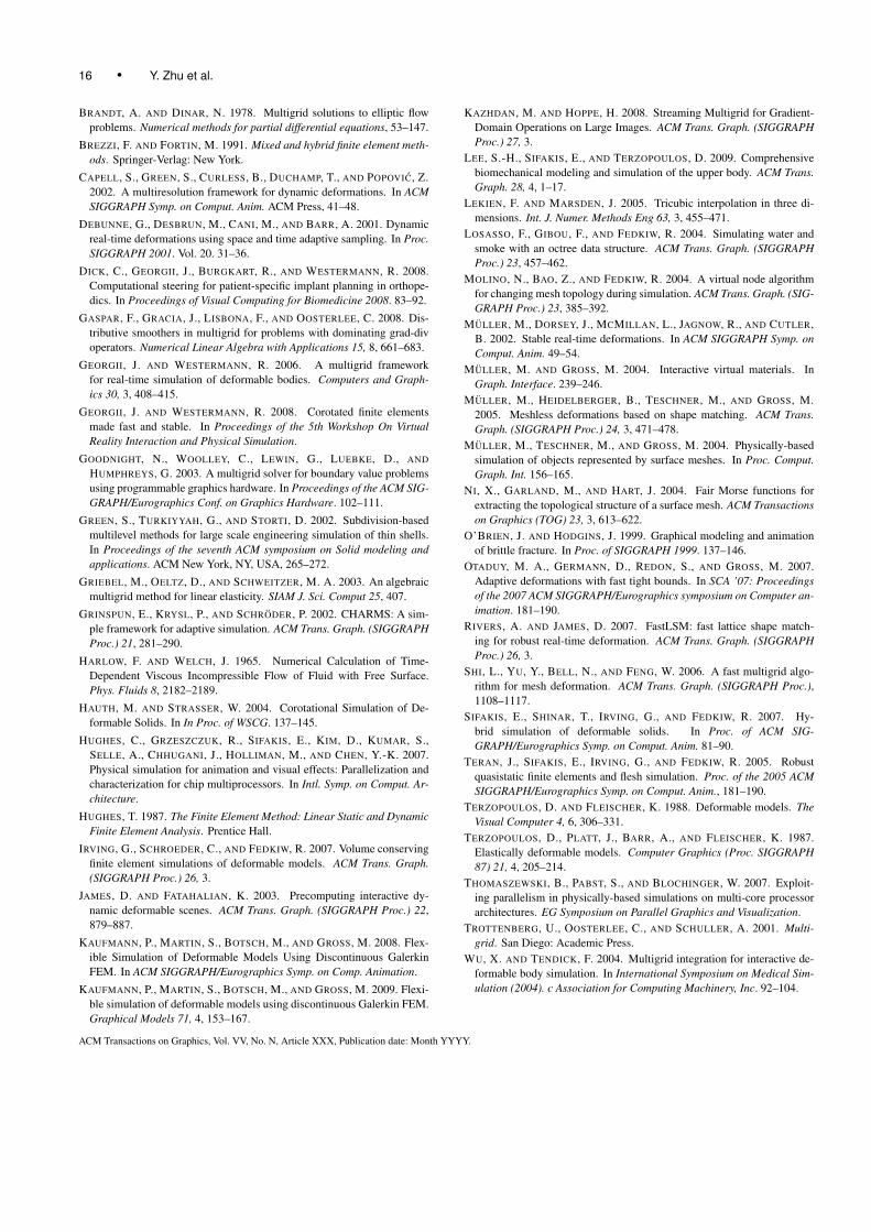
16 • Y. Zhu et al.
BRANDT, A. AND DINAR, N. 1978. Multigrid solutions to elliptic flowproblems. Numerical methods for partial differential equations, 53–147.
BREZZI, F. AND FORTIN, M. 1991. Mixed and hybrid finite element meth-ods. Springer-Verlag: New York.
CAPELL, S., GREEN, S., CURLESS, B., DUCHAMP, T., AND POPOVIC, Z.2002. A multiresolution framework for dynamic deformations. In ACMSIGGRAPH Symp. on Comput. Anim. ACM Press, 41–48.
DEBUNNE, G., DESBRUN, M., CANI, M., AND BARR, A. 2001. Dynamicreal-time deformations using space and time adaptive sampling. In Proc.SIGGRAPH 2001. Vol. 20. 31–36.
DICK, C., GEORGII, J., BURGKART, R., AND WESTERMANN, R. 2008.Computational steering for patient-specific implant planning in orthope-dics. In Proceedings of Visual Computing for Biomedicine 2008. 83–92.
GASPAR, F., GRACIA, J., LISBONA, F., AND OOSTERLEE, C. 2008. Dis-tributive smoothers in multigrid for problems with dominating grad-divoperators. Numerical Linear Algebra with Applications 15, 8, 661–683.
GEORGII, J. AND WESTERMANN, R. 2006. A multigrid frameworkfor real-time simulation of deformable bodies. Computers and Graph-ics 30, 3, 408–415.
GEORGII, J. AND WESTERMANN, R. 2008. Corotated finite elementsmade fast and stable. In Proceedings of the 5th Workshop On VirtualReality Interaction and Physical Simulation.
GOODNIGHT, N., WOOLLEY, C., LEWIN, G., LUEBKE, D., AND
HUMPHREYS, G. 2003. A multigrid solver for boundary value problemsusing programmable graphics hardware. In Proceedings of the ACM SIG-GRAPH/Eurographics Conf. on Graphics Hardware. 102–111.
GREEN, S., TURKIYYAH, G., AND STORTI, D. 2002. Subdivision-basedmultilevel methods for large scale engineering simulation of thin shells.In Proceedings of the seventh ACM symposium on Solid modeling andapplications. ACM New York, NY, USA, 265–272.
GRIEBEL, M., OELTZ, D., AND SCHWEITZER, M. A. 2003. An algebraicmultigrid method for linear elasticity. SIAM J. Sci. Comput 25, 407.
GRINSPUN, E., KRYSL, P., AND SCHRODER, P. 2002. CHARMS: A sim-ple framework for adaptive simulation. ACM Trans. Graph. (SIGGRAPHProc.) 21, 281–290.
HARLOW, F. AND WELCH, J. 1965. Numerical Calculation of Time-Dependent Viscous Incompressible Flow of Fluid with Free Surface.Phys. Fluids 8, 2182–2189.
HAUTH, M. AND STRASSER, W. 2004. Corotational Simulation of De-formable Solids. In In Proc. of WSCG. 137–145.
HUGHES, C., GRZESZCZUK, R., SIFAKIS, E., KIM, D., KUMAR, S.,SELLE, A., CHHUGANI, J., HOLLIMAN, M., AND CHEN, Y.-K. 2007.Physical simulation for animation and visual effects: Parallelization andcharacterization for chip multiprocessors. In Intl. Symp. on Comput. Ar-chitecture.
HUGHES, T. 1987. The Finite Element Method: Linear Static and DynamicFinite Element Analysis. Prentice Hall.
IRVING, G., SCHROEDER, C., AND FEDKIW, R. 2007. Volume conservingfinite element simulations of deformable models. ACM Trans. Graph.(SIGGRAPH Proc.) 26, 3.
JAMES, D. AND FATAHALIAN, K. 2003. Precomputing interactive dy-namic deformable scenes. ACM Trans. Graph. (SIGGRAPH Proc.) 22,879–887.
KAUFMANN, P., MARTIN, S., BOTSCH, M., AND GROSS, M. 2008. Flex-ible Simulation of Deformable Models Using Discontinuous GalerkinFEM. In ACM SIGGRAPH/Eurographics Symp. on Comp. Animation.
KAUFMANN, P., MARTIN, S., BOTSCH, M., AND GROSS, M. 2009. Flexi-ble simulation of deformable models using discontinuous Galerkin FEM.Graphical Models 71, 4, 153–167.
KAZHDAN, M. AND HOPPE, H. 2008. Streaming Multigrid for Gradient-Domain Operations on Large Images. ACM Trans. Graph. (SIGGRAPHProc.) 27, 3.
LEE, S.-H., SIFAKIS, E., AND TERZOPOULOS, D. 2009. Comprehensivebiomechanical modeling and simulation of the upper body. ACM Trans.Graph. 28, 4, 1–17.
LEKIEN, F. AND MARSDEN, J. 2005. Tricubic interpolation in three di-mensions. Int. J. Numer. Methods Eng 63, 3, 455–471.
LOSASSO, F., GIBOU, F., AND FEDKIW, R. 2004. Simulating water andsmoke with an octree data structure. ACM Trans. Graph. (SIGGRAPHProc.) 23, 457–462.
MOLINO, N., BAO, Z., AND FEDKIW, R. 2004. A virtual node algorithmfor changing mesh topology during simulation. ACM Trans. Graph. (SIG-GRAPH Proc.) 23, 385–392.
MULLER, M., DORSEY, J., MCMILLAN, L., JAGNOW, R., AND CUTLER,B. 2002. Stable real-time deformations. In ACM SIGGRAPH Symp. onComput. Anim. 49–54.
MULLER, M. AND GROSS, M. 2004. Interactive virtual materials. InGraph. Interface. 239–246.
MULLER, M., HEIDELBERGER, B., TESCHNER, M., AND GROSS, M.2005. Meshless deformations based on shape matching. ACM Trans.Graph. (SIGGRAPH Proc.) 24, 3, 471–478.
MULLER, M., TESCHNER, M., AND GROSS, M. 2004. Physically-basedsimulation of objects represented by surface meshes. In Proc. Comput.Graph. Int. 156–165.
NI, X., GARLAND, M., AND HART, J. 2004. Fair Morse functions forextracting the topological structure of a surface mesh. ACM Transactionson Graphics (TOG) 23, 3, 613–622.
O’BRIEN, J. AND HODGINS, J. 1999. Graphical modeling and animationof brittle fracture. In Proc. of SIGGRAPH 1999. 137–146.
OTADUY, M. A., GERMANN, D., REDON, S., AND GROSS, M. 2007.Adaptive deformations with fast tight bounds. In SCA ’07: Proceedingsof the 2007 ACM SIGGRAPH/Eurographics symposium on Computer an-imation. 181–190.
RIVERS, A. AND JAMES, D. 2007. FastLSM: fast lattice shape match-ing for robust real-time deformation. ACM Trans. Graph. (SIGGRAPHProc.) 26, 3.
SHI, L., YU, Y., BELL, N., AND FENG, W. 2006. A fast multigrid algo-rithm for mesh deformation. ACM Trans. Graph. (SIGGRAPH Proc.),1108–1117.
SIFAKIS, E., SHINAR, T., IRVING, G., AND FEDKIW, R. 2007. Hy-brid simulation of deformable solids. In Proc. of ACM SIG-GRAPH/Eurographics Symp. on Comput. Anim. 81–90.
TERAN, J., SIFAKIS, E., IRVING, G., AND FEDKIW, R. 2005. Robustquasistatic finite elements and flesh simulation. Proc. of the 2005 ACMSIGGRAPH/Eurographics Symp. on Comput. Anim., 181–190.
TERZOPOULOS, D. AND FLEISCHER, K. 1988. Deformable models. TheVisual Computer 4, 6, 306–331.
TERZOPOULOS, D., PLATT, J., BARR, A., AND FLEISCHER, K. 1987.Elastically deformable models. Computer Graphics (Proc. SIGGRAPH87) 21, 4, 205–214.
THOMASZEWSKI, B., PABST, S., AND BLOCHINGER, W. 2007. Exploit-ing parallelism in physically-based simulations on multi-core processorarchitectures. EG Symposium on Parallel Graphics and Visualization.
TROTTENBERG, U., OOSTERLEE, C., AND SCHULLER, A. 2001. Multi-grid. San Diego: Academic Press.
WU, X. AND TENDICK, F. 2004. Multigrid integration for interactive de-formable body simulation. In International Symposium on Medical Sim-ulation (2004). c Association for Computing Machinery, Inc. 92–104.
ACM Transactions on Graphics, Vol. VV, No. N, Article XXX, Publication date: Month YYYY.
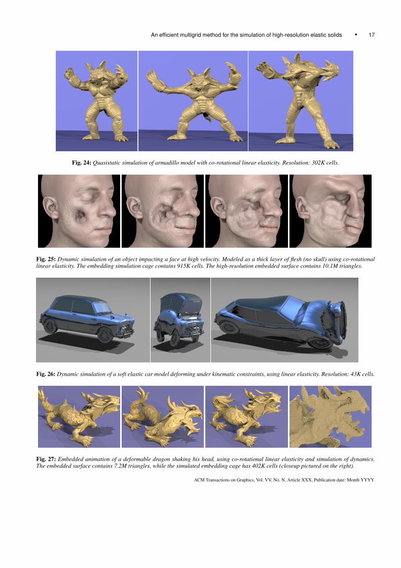
An efficient multigrid method for the simulation of high-resolution elastic solids • 17
Fig. 24: Quasistatic simulation of armadillo model with co-rotational linear elasticity. Resolution: 302K cells.
Fig. 25: Dynamic simulation of an object impacting a face at high velocity. Modeled as a thick layer of flesh (no skull) using co-rotationallinear elasticity. The embedding simulation cage contains 915K cells. The high-resolution embedded surface contains 10.1M triangles.
Fig. 26: Dynamic simulation of a soft elastic car model deforming under kinematic constraints, using linear elasticity. Resolution: 43K cells.
Fig. 27: Embedded animation of a deformable dragon shaking his head, using co-rotational linear elasticity and simulation of dynamics.The embedded surface contains 7.2M triangles, while the simulated embedding cage has 402K cells (closeup pictured on the right).
ACM Transactions on Graphics, Vol. VV, No. N, Article XXX, Publication date: Month YYYY.