Efficient Computation of Closed Contours using Modified Baum-Welch Updating

Leigh. A. Johnston and James. H. ElderCentre for Vision Research

York University, Toronto, Canada

AbstractWe address the problem of computing closed contours delin-eating the boundaries of objects of interest from image tan-gent maps. The Bayesian formulation of this problem incor-porates the notion of foreground and background models ininferring the optimal image organization. Due to vital non-local constraints, the optimal MAP solution is intractable.We present a novel efficient search algorithm for the con-struction of highly probable closed contours, based on theBaum-Welch algorithm for updating hidden Markov modelparameters.

1 IntroductionPerceptual organization can be treated probabilistically,making use of appropriate Bayesian frameworks [1, 2, 3, 4].We follow here the maximum a posteriori (MAP) formu-lation advanced in [4], incorporating Markov assumptions,grouping cues and object knowledge for the contour group-ing task. Non-local constraints such as contour closure,simplicity (non-self-intersection) and global priors prohibitthe exact solution of the MAP objective. Standard dynamicprogramming search techniques that rely on local Markovassumptions cannot guarantee the optimality or simplicityof the computed closed contours. Further, while these stan-dard algorithms have polynomial time complexity, they re-main too computationally expensive for larger images. Effi-cient, approximate search techniques suited to this problemare therefore of great interest.

Prior approaches to computing closed contours gener-ally fail to take into account important global constraints(though see Jacobs [5] for a global approach restricted toconvex groups). The approach of Elder and Zucker [2] com-putes complete contours in polynomial time but does notincorporate the simplicity constraint or global priors. Themethod of Thornber and Williams for segmenting closedcontours [6, 7] also has no means to incorporate these con-straints, nor does it model the background distribution.

The novel search algorithm we propose for Bayesianconstruction of closed contours overcomes the limitationsof previous approaches in its ability to incorporate non-local constraints, and outperforms existing [4] and naive

approaches. In [4] a greedy algorithm for contour con-struction is implemented that monotonically grows a set ofhighly probable, simple contours, pruning the least proba-ble at each step to respect memory and time bounds. Thisalgorithm can fail for complex problems due to overprun-ing. Empirically, we have observed that intermediate con-tour hypotheses tend to cluster into minor variants of eachother, which fail to grow into the correct complete bound-ary. Thus the algorithm locks on prematurely to a highlypeaked local maximum in the high-dimensional space ofcontour hypotheses. Superior performance of the new al-gorithm proposed here derives from two key features:

• A more evenly distributed sampling of the contourhypothesis space is enforced by restricting the firsttwo tangents of each contour hypothesis to be unique.

• A heuristic, based on the Baum-Welch algorithm forparameter estimation of hidden Markov models [8], isemployed that acts as a look-ahead mechanism and in-fluences the contour hypotheses toward closure.

Combinatorial problems formulated using Bayesianmodels often result in the optimization of a maximum sum-cost objective, for which the class of A* heuristic algo-rithms is applicable [9]. A* algorithms choose paths toexplore in a graph based on a path weight that is a com-bination of (i) the cumulative cost of the current path, and(ii) the heuristic look-ahead cost of reaching the goal statefrom the current path.

There are two classes of A* heuristics: admissibleheuristics, that guarantee convergence to the optimal solu-tion, and inadmissible heuristics, that do not. In practice,inadmissible heuristics are often preferred due to their fasterconvergence properties [9]. For the problem of computingclosed contours, we have no choice: non-local constraintsnecessitate inadmissible heuristics.

A* algorithms have been employed previously in per-ceptual organization, however not with dynamic look-aheadheuristics capable of learning from past decisions. Gemanand Jedynak [10] studied the problem of road tracking insatellite imagery, applying a tree search algorithm based onan entropy testing rule to determine which paths to explore.

1

Yuille and Coughlan proved that this algorithm is a variantof an inadmissible A* algorithm with no heuristic weight-ing term [9]. Thus the Geman and Jedynak algorithm andits variants are essentially greedy shortest-path algorithms.

Yuille and Coughlan present measures for quantify-ing the performance of A* algorithms for Bayesian infer-ence [11], however these results depend on the underlyingprobability distributions being shift-invariant Markov. Thenon-local contour grouping constraints invalidate the appli-cation of their results to the perceptual organization taskstudied here.

Methods for optimizing saliency networks based on ge-ometric properties of contour elements are based on theformation of contours that tend to close [12], salient con-vex contours [5], and closed contours formed via heuristicsearch strategies that give preference to contours satisfyingglobal geometric salience measures [13]. The salience mea-sures we use are based on probabilistic models of both geo-metric and photometric properties of the contour elements,and the measure of closure used to drive the dynamic heuris-tic search algorithm is formally grounded in the theory ofhidden Markov models.

The AI literature contains examples of dynamic heuris-tic search algorithms that learn from previous decisions,termed incremental search or replanning algorithms [14].The D* (Dynamic A*) algorithm [15] is perhaps thefirst such incremental search algorithm, although dynamicshortest-path algorithms have been proposed since the late1960s [14]. These algorithms, largely used for mobilerobotics, are dynamic search procedures that adapt andmake use of previous decisions as the system parametersand costs change. The perceptual organization problem weaddress here is different in that the costs are static but non-local.

In this paper, we address the problem of computing theboundary of a single object of interest, based on both gen-eral purpose grouping cues and object-specific knowledge.Images are represented by their tangent maps [2], and dis-tributions of object cues associated with individual tangentsand grouping cues associated with tangent pairs are learnedfrom training images. In Sec. 5 we extend the proposed al-gorithm to deal with multiple objects of interest.

The paper proceeds as follows. Notation is described inSec. 2, followed by the Bayesian problem formulation andMAP objective in Sec. 3. The proposed constructive algo-rithm is then derived and presented in Sec. 4, together withits relationship to the Baum-Welch algorithm for parameterestimation of hidden Markov models. Sec. 5 demonstratesthe effectiveness of the algorithm.

2 Notation

We follow the convention that capitalized letters, Z, denotesets, script upper case letters, Z , denote random variables,bold-faced upper case letters, Z, denote matrices, lowercase letters, z, denote realizations of random variables, andbold-faced lower case letters, z, denote vectors.

Image contours are locally represented by variablelength tangents, formed by the grouping of local edges intoshort linear segments. The edge elements are first detectedby a multiscale edge detection algorithm [16]. The resul-tant tangent map is a set of N tangents, T = {t1, . . . , tN},where each ti indexes a point in the space of observabletangents.

Define S to be a length-m sequence of random variableswith components, Sk ∈ T, ∀ k = 1, . . . ,m. A length-mcontour, s = [tα1 , . . . , tαm

], is a realization of S for whichαi 6= αj ∀ i ∈ {1, . . . ,m}, j ∈ {2, . . . ,m − 1}, i 6= j.The set of all possible contours is denoted by S. Similarly,the set of all possible closed contours, S∗ ⊂ S, is all s forwhich s ∈ S and tα1 = tαm

.It is assumed that there exists a correct organization of

the image, C ⊂ S. All tangent sequences corresponding toactual contours in the image and the subsequences thereofare contained in C. The set of object fragments, So, is de-fined as s ∈ So iff tαi

∈ T o ∀ i ∈ {1, . . . ,m}, where T o

is the set of tangents on the boundary of the object of inter-est. We define the set of object contours, Co, as the set ofcorrectly organized object fragments, Co = So ∩ C. Theobject boundary, co∗ ∈ Co ∩S∗, and all object contours areassumed to be simple (not self-intersecting).

The set of observed data, D = Do ∪ Dc, is comprisedof the set of observable object cues,Do, and grouping cues,Dc. Do determines the likelihood that tangents lie on theboundary of the object of interest, while Dc determines thelikelihood that pairs of tangents should be grouped together.Each element of the object cue set, di ∈ Do, is a set of loobservations about tangent ti. Similarly, each element ofthe grouping cue set, dij ∈ Dc, i 6= j, is composed of lcobservations about the tangent pair tij .

The grouping cues, dij , are general purpose relation-ships between pairs of tangents, such as brightness, con-trast, proximity and good continuation. The object cues, di,are specific to the object of interest. For the satellite lakeimages shown in Fig. 3, the object cues are the tangent’sdark side intensity and the distance to the nearest tangentin the direction opposite to the local intensity gradient, i.e.,toward the interior of the lake for object tangents.

It is assumed that the local cues, di and dij , are indepen-dent of cues pertaining to other tangents or tangent pairs,when conditioned upon a contour hypothesis, s ∈ Co. It isalso assumed that local cues are independent of all compo-nents of a contour hypothesis except the tangent or tangent

2

pair to which they directly pertain.The problem space forms a sparsely-connected graph, as

only the strongest grouping hypotheses within a limited ra-dius around each tangent are considered. For each ti ∈ T ,we define a set of tangents, Gi = {tj}, whose |Gi| = gelements group most strongly to ti, as measured by the lo-cal probabilities p({ti, tj} ∈ C | dij)× p(tj ∈ T o | dj). Wesearch tangents within a radius of rg pixels, to reduce thecomputation required in constructing the sparse graph.

3 Theory

The objective can be formulated as a maximum a posteriori(MAP) inference problem,

co∗ = arg maxs∈S∗

p(s = co∗|D) (1)

Under the data independence assumptions (Sec. 2), p(s =co∗|D), can be decomposed into the product of a fore-ground, background and global prior term [4],

p(s = co∗|D) ∝ F ∗(s, D)B∗(s, D)P ∗(s) (2)

where, for s = [tα1 , . . . , tαm],

F ∗(s, D) =

m∏

k=1

p(dαk| tαk

∈ T o)

p(dαk)

(3)

×m−1∏

k=1

p(dαkαk+1| {tαk

, tαk+1} ∈ C)

p(dαkαk+1)

B∗(s, D) =∏

{i:ti /∈s}

p(di|ti /∈ T o)

p(di)(4)

P ∗(s) = p(s = co∗) (5)

Thus the foreground term is concerned with the tangents onthe boundary of the object of interest, while the backgroundterm models tangents that are inside or outside the objectboundary.

Somewhat surprisingly, the posterior probability of anobject contour, p(s ∈ Co|D), can be expressed as a productof local object and pairwise grouping posterior probabili-ties [4],

p(s ∈ Co|D) ∝m∏

k=1

p(tαk∈ T o|dαk

) (6)

×m−1∏

k=1

p({tαk, tαk+1

} ∈ C | dαkαk+1)

where, by application of Bayes’ theorem, the local posteri-

ors are

p(tαk∈ T o|dαk

) =p(dαk

| tαk∈ T o) p(tαk

∈ T o)

p(dαk)

(7)

p({tαk, tαk+1

} ∈ C | dαkαk+1)

=p(dαkαk+1

| {tαk, tαk+1

} ∈ C) p({tαk, tαk+1

} ∈ C)

p(dαkαk+1)

(8)

A comparison between the foreground term (3) and the ob-ject contour posterior (6) reveals the following relationship,

F ∗(s, D) = (popc)−m Ψ(s,dos,dc

s) (9)

p(s ∈ Co|D) ∝ Ψ(s,dos,dc

s) (10)

where

Ψ(s,dos ,d

cs) =

m∏

k=1

p(tαk∈ T o|dαk

) (11)

×m−1∏

k=1

p({tαk, tαk+1

} ∈ C | dαkαk+1)

po = p(tαk∈ T o), pc = p({tαk

, tαk+1} ∈ C) (12)

dos

= [dα1 , . . . , dαm], dc

s= [dα1α2 , . . . , dαm−1αm

](13)

Eqns. (9)–(10) indicate that a contour with high p(s ∈Co|D) will also have a high foreground probability term,F ∗(s, D), relative to other contours of the same length. Wetherefore follow the approach outlined in [4] and constructa set of closed contours, C∗, that have high Ψ(s,do

s ,dcs).

Eqns. (3)–(5) are then used to select from C∗ the most prob-able object boundary.

The success of the procedure in determining the contourthat maximizes the MAP objective rests on the ability of theconstructive algorithm to produce a set of closed contoursthat are highly probably object contours. In Sec. 4 we derivea new algorithm, based on an optimal parameter estimationalgorithm for hidden Markov models (HMMs), that uses alook-ahead heuristic to determine contour closure.

4 New algorithm

The set of closed contours, C∗, from which the contourwith the maximum p(s = co∗|D) is chosen, is constructedthrough a contour growth procedure that iteratively extendsa set of highly probable tangent sequences, pruning thoseless likely to be valid object contours. Closed contours aris-ing during the procedure are stored, forming C∗.

The object contour posterior (10) is a product of localprobabilities, reflecting both the data independence assump-tions, and the assumption of local priors (12). In the ab-sence of self-intersection restrictions, the problem of deter-mining the contour most likely to be an object contour can

3

be solved via standard dynamic programming techniques inpolynomial time [2]. The restriction that contours be sim-ple renders the problem exponentially complex, as completecontour histories are required when constructing candidatecontours.

Consider the application of an all-pairs-shortest-path(APSP) algorithm to the test image depicted in the bottomrow of Fig. 3. The optimal contour, taking 392 minutesto determine, is simple (similar to the bottom-left image inFig. 3, for space reasons omitted), however there is no guar-antee of this in general. The APSP algorithm determines,for each tangent, the closed contour that maximizes theforeground probability (9). There is no guarantee that a con-tour maximizing (9) will also maximize the posterior (1).Indeed, the optimal closed contour obtained by the APSPalgorithm has a lower global posterior probability than theclosed contour computed via the proposed MBW algorithm(Fig. 3). The computational complexity of the APSP algo-rithm is O(N2g +N2 logN)), where g = |Gi| is the num-ber of continuations considered from each tangent (Sec. 2).The images we test have between 2000 and 40000 tangents,making application of the APSP algorithm computationallyinfeasible for any but the smallest images. The 392 minuterun-time of the APSP algorithm for the small, 4414 tangentimage in the top row of Fig. 3 stands in direct contrast tothe low run-times of the efficient algorithms proposed andcompared within this paper.

In our proposed Modified Baum-Welch (MBW) algo-rithm a set of length-2 contours is first instantiated togetherwith the set of associated object contour probabilities. Thecontours in the set are then grown iteratively by greedydecision-making based on a novel look-ahead heuristic thatinfluences the contours toward closure. The object contourprobabilities, upon which the look-ahead heuristic weightsare based, are updated as the contours grow, and any closedcontours that form in the growth process are stored sepa-rately in C∗. A contour’s growth is terminated when thereis no simple tangent extension available, i.e. all extensionscause self-intersections. When no contours remain unter-minated, or a predefined maximum contour length, L, hasbeen reached, the MBW algorithm stops, at which point theMAP objective (1) is evaluated over the set C∗ to determinethe optimal contour. The computational complexity of theMBW algorithm is O(NgL2). For constants g, L << N ,this algorithm is considerably more efficient.

We now formalize the MBW algorithm, deriving thecontour HMM in Sec. 4.1, and its relationship to the objectcontour posterior, p(s ∈ Co|D). Sec. 4.2 then demonstratesthe use of estimates of high-order Markov transition prob-abilities as look-ahead heuristics for the MBW algorithm’sgrowth mechanism, and the relationship between the Baum-Welch and proposed MBW algorithms.

4.1 Object contour hidden Markov modelFor notational simplicity and completeness in describing ahidden Markov model of object contours, we make the fol-lowing definitions. Define the length-m sequence of ran-dom variables, Do, with components Do

k defined on thediscrete sample space of observed object cues. That is,Do

k ∈ Do, ∀k = 1, . . . ,m. Associate the sequence Do

with the tangent sequence S (defined in Sec. 2), such thatthe assignment Sk = tαk

implies Dok = dαk

.Similarly, define Dc to be the length-(m− 1) sequence

of random variables with components Dck defined on the

discrete sample space of observed grouping cues, Dck ∈

Dc, ∀k = 1, . . . ,m − 1. Associate Dc with S such thatSk = tαk

and Sk+1 = tαk+1implies Dc

k = dαkαk+1.

Associate also with S the sequences of random variables,X and Y , of lengths m and (m − 1) respectively. Let thecomponents of X be binary-valued random variables, Xk ∈{x+, x−}, that label S; for Sk = tαk

, the realization Xk =x+ is shorthand for tαk

∈ T o, and Xk = x− is shorthandfor tαk

/∈ T o. Let the components of Y be binary-valuedrandom variables, Yk ∈ {y+, y−}, that also label S. ForSk = tαk

and Sk+1 = tαk+1, Yk = y+ is shorthand for

{tαk, tαk+1

} ∈ C, and similarly Yk = y− is shorthandfor {tαk

, tαk+1} /∈ C. Define the particular realizations,

x+ = [x+, . . . , x+] and y+ = [y+, . . . , y+], of lengths mand m− 1 respectively.

Under this notation, the local object and grouping poste-riors (7)–(8) are expressed as

p(Xk = x+ | Dok = dαk

) = p(tαk∈ T o | dαk

) (14)

p(Yk = y+ | Dck = dαkαk+1

) = p({tαk, tαk+1

} ∈ C | dαkαk+1)

Recall from (9)–(10) that for contours of equal length, theposterior probability of an object contour hypothesis, p(s ∈Co|D), is proportional to the product of local posteriors,Ψ(s,do

s ,dcs). Under the new notation, this product is

Ψ(s,dos ,d

cs) = p(X = x+|Do = do

s) p(Y = y+|Dc = dcs)

(15)

where

p(X = x+|Do = dos) =

m∏

k=1

p(Xk = x+|Dok = dαk

) (16)

p(Y = y+|Dc = dcs) =

m−1∏

k=1

p(Yk = y+|Dck = dαkαk+1

)

(17)

The MBW algorithm seeks contours, s, with highΨ(s,do

s,dc

s). This then defines an optimization of the func-

tion Ψ(s,dos ,d

cs) over all valid realizations of the discrete

random variable sequence, S = s, and the subsequently de-termined sequences of discrete random variables, Do = do

s,

4

and Dc = dcs. From (15) it is evident that for any two

equal-length realizations, s1 and s2, Ψ(s1,dos1,dc

s1) and

Ψ(s2,dos2,dc

s2) differ only in the variables on which we

are conditioning, while the label sequences, X = x+ andY = y+, remain fixed. Therefore we can conceptualizex+ and y+ to be data sequences, and {s,do

s,dc

s} to be se-

quences of state variables to be estimated. This interpreta-tion renders Ψ(s,do

s,dc

s) a product of local likelihood func-

tions, rather than local posteriors, which can be precom-puted on the discrete sample spaces, T,Do and Dc. Theselocal likelihood functions form the emission distribution ofthe proposed HMM.

The relationships between the sequences of random vari-ables are depicted in Bayes network form in Fig. 1. Thelinking of consecutive states in the tangent sequence, S,implies the Markovian dependence of the tangent in posi-tion k in the sequence on the tangent in position k − 1. Infact, Fig. 1 defines a hidden Markov model, M, with states,Sk, ranging over the discrete state space, T , and emittedsymbols, Xk and Yk, related via the likelihood distribution,Ψ(S,Do,Dc).

� ��

� ��

� ��

� ��

� ��

� ��

� ��

� ��

� ��

� ��

� ��

??

ZZ

ZZ~ ?

��

��=?

?

ZZ~

?

?

��=

- - -

Xm

Do

2

X2

Do

mDc

1

Y1

S1 S2 Sm

X1

Do

1

Figure 1: Bayes network depicting the contour hiddenMarkov model, M. The first-order Markov dynamics ofthe tangent sequence, S, are indicated by the directed linksbetween consecutive sequence elements.

It is therefore possible to define a constructive algorithmobjective, related to the maximization of Ψ(s,do

s,dcs), on

the posterior,

pM(S = s | X = x+,Y = y+)

∝ p(X = x+,Y = y+ | Do = dos ,D

c = dcs)

× pM(Do = dos,Dc = dc

s| S = s) pM(S = s)

= p(X = x+,Y = y+ | Do = dos ,D

c = dcs) pM(S = s)

= Ψ(s,dos,dc

s) pM(S = s) (18)

where the deterministic mapping from tangent to cue se-quences, that renders pM(Do = do

s,Dc = dc

s| S = s) = 1,

simplifies the expression, and the first-order Markov prioras specified in the Bayes network in Fig. 1 is pM(S) =∏m

k=2 pM(Sk|Sk−1) pM(S1). We define notation for the

homogeneous transition probabilities:

aij = pM(Sk = tj | Sk−1 = ti), ∀ ti ∈ T, j ∈ Gi (19)

If the HMM for object contours is assumed to haveequiprobable initial state and transition probabilities, thenmaximizing the posterior (18) is equivalent to maximiz-ing Ψ(s,do

s ,dcs). The constructive algorithm presented

in [4] is therefore a suboptimal maximum likelihood se-quence estimation algorithm, as it bases contour growthsolely on Ψ(s,do

s ,dcs). The MBW algorithm we derive

here is based on the full posterior (18), using estimates ofthe prior pM(S = s) to dynamically effect contour growthtowards closure.

4.2 Transition probabilities and closureThe assumption of first-order Markov contour dynamics,though helpful as a simplifying approximation for the con-struction of candidate contours, does not take into accountglobal constraints. As the objective of the contour con-struction algorithm is to form a set of closed contours,pM(Sk = tαk

|Sk−1 = tαk−1, . . . ,S1 = tα1) cannot be

independent of S1 = tα1 . Similarly, satisfying the re-quirement that contours not self-intersect demands the en-tire sequence history in determining pM(Sk = tαk

|Sk−1 =tαk−1

, . . . ,S1 = tα1). The greedy mechanism of the pro-posed MBW algorithm influences contour growth towardsclosure by application of a heuristic term based on estimatesof joint state transition probabilities, pM(S+,S2|S1), where+ is used to indicated a sequence position index greater than2.

In a greedy construction of candidate closed contours,open contours are grown tangent-by-tangent in the searchfor closed contours. At iteration k, a length-k contour, s1,is extended to s2 = [s1, tβ]. Define label sequences, x+

2

and y+2 , to be of the same length as s2. A greedy algorithm

based solely on maximizing the posterior, pM(S = s2|X =x+

2 ,Y = y+2 ), under the assumption of equiprobable tran-

sition probabilities, would choose tαk+1such that

tαk+1= arg max

tβ∈Gαk

pM(S = s2|X = x+2 ,Y = y+

2 )

= arg maxtβ∈Gαk

pM(S = s1|X = x+1 ,Y = y+

1 )

× ψk(tαk, tβ) pM(Sk+1 = tβ |Sk = tαk

)

= arg maxtβ∈Gαk

ψk(tαk, tβ) pM(Sk+1 = tβ |Sk = tαk

)

(20)

Rather than basing greedy decisions purely on local likeli-hood values, ψk(·), the proposed MBW algorithm weightsthe potential contour continuations according to estimatesof the probability that the extended contour will returnto the initial tangent at some future iteration. Let S =

5

[S1, . . . ,Sk,Sk+1], and S ′ = [S,Sk+2, . . . ,S+, . . .]. Thenthe chosen continuation tαk+1

is given by

tαk+1= arg max

tβ∈Gαk

pM(S = s2,S+ = tα1 |X = x+2 ,Y = y+

2 )

= arg maxtβ∈Gαk

ψk(tαk, tβ)pM(Sk+1 = tβ ,S+ = tα1 |Sk = tαk

)

The heuristic weighting terms, pM(Sk+1,S+|Sk), are jointstate transition probabilities, estimates of which are ob-tained via a modified Baum-Welch algorithm.

The Baum-Welch algorithm (BWA) is an instance of theExpectation-Maximization algorithm for the estimation ofhidden Markov model parameters [8]. It is an iterative pro-cedure guaranteed to converge to a local maximum on thelikelihood surface, p(X = x+,Y = y+|A), in the absenceof contour closure or simplicity assumptions that invalidatethe first-order Markov assumption. The parameters of themodel, M, optimized by the BWA are the transition proba-bilities, A, with elements defined in (19). The initial transi-tion probability estimates, A(1), are set to be equiprobable.The E and M steps of the BWA proceed as follows.

• E step: Form joint state probabilities conditioned onthe object contour hypothesis and current transitionprobability estimates, A(n). For k ∈ [1,m], ti ∈T, tj ∈ Gi:

γ(n)k (ti, tj) = pA(Sk−1 = ti,Sk = tj | X = x+,Y = y+,A(n))

=∑

S=s:Sk−1=ti,Sk=tj

Ψ(s,dos,dc

s) p

A(n)(S = s)

The joint state probabilities arise from the standardEM procedure of forming the auxiliary function,ES{log p(S,X ,Y|A) |x+,y+, A(n)}, where ES{·}denotes expectation with respect to the random vari-ables S. For an instructive derivation of the Baum-Welch update equations, see [17].

• M step: Update the transition probability estimates,A(n+1) = [a

(n+1)ij ], ∀{i, j} : ti ∈ T, tj ∈ Gi:

a(n+1)ij =

(

m∑

k=1

γ(n)k (ti, tj)

)/(

m∑

k=1

∑

tj′∈Gi

γ(n)k (ti, tj′ )

)

The E step computes the sum of a number of terms ex-ponential in the sequence length, however the forwards-backwards algorithm [8] performs this computation in poly-nomial time. The contour simplicity constraint violatesthe first-order Markov assumption, and thus determiningp(Sk|Sk−1, . . . ,S1) demands the entire sequence history.Therefore, exact computation of the E step requires in-tractable memory and computational power. The MBW im-plements a sequential, approximate BWA, replacing the E

step sum with a max operator, and iterating over succes-sively longer sequences of random variables. The secondmodification that the MBW algorithm makes is to use esti-mates, aijl, of high-order joint state transition probabilities,pA(Sk+1 = tj ,S+ = tl | Sk = ti), rather than the first-order transition probabilities, pA(Sk+1 = tj |Sk = ti). Thejoint state transition probabilities are used to influence con-tour closure, as previously discussed in this section.

The transition probabilities, A(1) = [a(1)ij ], are initialized

as equiprobable, a(1)ij = 1/g (recall g = |Gi|). The MBW

also requires both the initialization of the set of all length-2contours, {s(1)

ij = [ti, tj ], ∀ ti ∈ T, tj ∈ Gi}, and the set of

joint state probabilities, {γ(1)ij = 1, ∀ ti ∈ T, tj ∈ Gi}.

• Modified E step: Form joint state probabilities condi-tioned on the object contour hypothesis and transitionprobability estimates, A(k). Store the extended con-tours associated with the joint state probabilities:

s(k)ij = [s

(k−1)ij , tαk+1

]

γ(k)ij ≈ γ

(k−1)ij ψk(tαk

, tαk+1) aαkαk+1i

where tαk= tail (s(k−1)

ij )

tαk+1= arg max

tβ∈Gαk

ψk(tαk, tβ) aαkβi

aαkβi =

{

a(k)αkβ , if ti ∈ s

(k−1)αkβ (contour closure)

1g , otherwise

• Modified M step: Update the transition probabilityestimates, A(k+1) = [a

(k+1)ij ], ∀ {i, j} : ti ∈ T, tj ∈

Gi:

a(k+1)ij = γ

(k)ij

/(

∑

j′∈Gi

γ(k)ij′

)

(21)

While the modifications made to the standard BWA denythe MBW proven convergence properties, the derivation ofthe MBW algorithm from this optimal parameter estimationalgorithm formally grounds the choice of heuristic.

The MBW algorithm in its entirety is stated in Fig. 2.

5 ResultsThe MBW algorithm differs from the constructive, greedyalgorithm presented in [4] through the reweighting ofMarkov transition probabilities and the even sampling ofcontours across the contour hypothesis space. In this sectionwe contrast the performances of these two algorithms, alongwith the performance of the algorithm that, like the MBWalgorithm, evenly samples the contour hypothesis space, butdoes not reweight transition probabilities. This algorithm isreferred to as the non-reweighted (NRW) algorithm.

6

The Modified Baum-Welch (MBW) Algorithm

Initialization: Initialize the following quantities:

• Tangent pair set, G ={

{ti, tj}, ∀ti ∈ T, tj ∈ Gi

}

.

• Closed contour set, C∗ = ∅.

• The sparse array of open contours, S(1), with elementss(1)ij = [ti, tj ], ∀{ti, tj} ∈ G.

• Joint state probability sparse array, Γ(1), with elementsγ

(1)ij = p(X1 = x+|Do

1 = di)ψ1(ti, tj), ∀{ti, tj} ∈ G.

• The sparse array of transition probabilities, A(1), withelements a(1)

ij = 1/g, ∀{ti, tj} ∈ G.

Recursion: For k = 2, 3, . . .

• Update contours, S(k), and joint state probabilities,Γ(k) (Mod. E step) For all {ti, tj} ∈ G:

– Form the set S+ ={

[s(k−1)ij , tαk+1

],

∀ tαk+1∈ Gαk

, tαk= tail (s(k−1)

ij )}

.

– Store in C∗ any s ∈ S+ that is closed and simple.

– If no simple and open contours result, remove{ti, tj} from G.

– Else, update both the open contour s(k)ij =

[s(k−1)ij , tαk+1

], and the joint state probability,

γ(k)ij = γ

(k−1)ij ψk(tαk

, tαk+1) aαkαk+1i, where

tαk+1= arg max

tβ∈Gαk

ψk(tαk, tβ) aαkβi,

tαk= tail (s(k−1)

ij )

aαkβi =

{

a(k)αkβ , if ti is in the contour s

(k−1)αkβ

1g , otherwise

• Update transition probs, A(k) (Mod. M step):

a(k+1)ij =

γ(k)ij

∑

tj′∈Gi

γ(k)ij′

, ∀ {ti, tj} ∈ G

Termination: G = ∅, or max contour length, L, reached.Output: The set of candidate MAP closed contours, C∗.

Figure 2: Details of the Modified Baum-Welch (MBW) al-gorithm for the construction of C∗.

Given unlimited tangent extension sets, g = |Gi|, andlarge memory budget to eliminate the effects of pruning,all three approaches would perform equally well. Here weadjust the size of g and the memory budget available, sepa-rately for each test image, to bring out the efficiency differ-ences of the algorithms. All three algorithms are given thesame g and the same memory budget for each image, andare tested on a 2.8GHz Pentium 4 machine.

We first evaluate algorithm performance on a set of fivepanchromatic IKONOS satellite images. In each image weseek the optimal closed contour bounding a lake. Two ob-ject cues, di, are used: the intensity on the dark side of tan-gent ti, and the distance between ti and the nearest tangentin the direction opposite to the local intensity gradient (to-ward the interior of the lake if ti is on the lake boundary).The four grouping cues, dij , considered are the distance be-tween the tangents ti and tj (proximity), the good contin-uation of the two tangents, approximated as the absolutevalue of the sum of the angles formed by a linear interpo-lation, the change in mean intensity (brightness) betweenthe two tangents, and the change in edge contrast betweenthe two tangents. The cue likelihood distributions are esti-mated from hand-segmented training data over five images,and modelled parametrically by generalized Laplacian dis-tributions [4].

Fig. 3 shows three test images for which the MBW suc-ceeds, while either the Greedy and/or NRW algorithmscompletely fail. In successful cases, the MBW’s contourshave a higher global posterior probability than the closedcontours produced by the other algorithms.

The MBW’s transition probability reweighting influ-ences the contours toward closure. Practically this resultsin candidate closed contour sets, C∗, that are larger thantheir counterparts resulting from the NRW algorithm, andthat contain a more diverse set of closed contours than inthe Greedy algorithm for which many closed contours dif-fer only by a small number of tangents. This may seemcounter-intuitive, as it may be expected that biasing towardclosure would lead to shorter, more direct paths being takentoward closure. However, as indicated in the recursive stepof the MBW algorithm (Fig. 2), for each remaining opencontour, the set, S+, is formed, from which the best opencontour extension is chosen to update the current contour,while any closed contours are stored. Thus while the pref-erence may be for shorter closed paths, by maintaining thebest open contours at each stage, there is no reduction inthe number of valid closed contours found at long contourlengths.

Figure 4 displays the results of repeated application of asingle-source shortest path algorithm (Dijkstra’s algorithm),initiated at the most probable tangent pair and then addi-tional pairs in descending order of probability, until themaximum running time of the MBW, Greedy and NRW al-

7

gorithms for each of the three test cases in Figure 3 is ex-ceeded. This approach succeeds in finding a lake boundaryin only one case.

Run time: 3.0 mins Run time: 5.6 mins Run time: 2.7 mins

Run time: 2.4 mins Run time: 7.3 mins Run time: 2.1 mins

Run time: 0.34 mins Run time: 0.33 mins Run time: 0.26 mins

Figure 3: Left: MBW, Middle: Greedy, Right: NRW. Toprow: g = 6, rg = 20, Middle, bottom rows: g = 5, rg = 10.

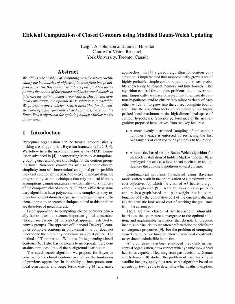
In our second experiment, we evaluated the algorithmson the problem of finding detailed bounding contours of ma-jor human skin regions in natural images (Fig. 5). We em-ployed the same grouping cues used in our first experiment,but considered only one object cue: the RGB colour of theskin and non-skin sides of skin boundary tangents. Again,the cue distributions are learned from five hand-segmentedtraining images taken in the test environment. To extendthe method to extract multiple skin regions from a singleimage, we employ an iterative procedure in which an op-timal closed contour is estimated, then removed from thetangent map.

Fig. 5 presents the results of the three algorithms for twotest images. In each case the MBW forms two closed con-tours delineating the two skin regions, while the Greedy al-gorithm fails to find one or both of the regions. The NRWalgorithm succeeds for the second image, but successfullyfinds only one of the skin regions in the first case, forminginstead a closed contour around part of the subject’s eye.Thus the MBW algorithm for computing closed contoursappears to be considerably more efficient than both purelygreedy and shortest-path approaches.

6 ConclusionsThe Modified Baum-Welch algorithm for the constructionof closed contours outlining object boundaries makes useof an even sampling of the contour hypothesis space and it-

Run time: 5.7 mins

Run time: 8.6 mins

Run time: 0.43 mins

Figure 4: Dijkstra’s algorithm, initialised at decreasinglylikely tangent pairs, run over time periods equal to or greaterthan the corresponding slowest times of the MBW, Greedyand NRW algorithms in Figure 3. Top: g = 6, rg = 20,Middle, bottom: g = 5, rg = 10.

erative reweighting of the Markov transition probabilitiesbased on the Baum-Welch updating mechanism, to formhighly probable closed contours. The MBW algorithm iscomputationally efficient, and has been shown to be morerobust than both the purely greedy approach presented in [4]and a naive non-reweighted version of the algorithm, in itsability to form closed contours given finite computationalresources.

References[1] I. J. Cox, J. M. Rehg, and S. Hingorani, “A Bayesian

multiple-hypothesis approach to edge grouping andcontour segmentation,” IJCV, vol. 11, pp. 5–24, 1993.

[2] J. H. Elder and S. W. Zucker, “Computing contour clo-sure,” in Proc. 4th ECCV, pp. 399–412, 1996.

[3] J. Sullivan, A. Blake, M. Isard, and J. Mac-Cormick, “Bayesian object localisation in images,”IJCV, vol. 44, no. 2, pp. 111–135, 2001.

[4] J. H. Elder, A. Krupnik, and L. A. Johnston, “Con-tour grouping with prior models,” IEEE Trans. PAMI,vol. 25, pp. 661–674, June 2003.

[5] D. Jacobs, “Robust and efficient detection of salientconvex groups,” IEEE Trans. PAMI, vol. 18, pp. 23–37, Jan. 1996.

8

Run time: 7.5 mins Run time: 40.0 mins Run time: 6.5 mins

Run time: 9.9 mins Run time: 44.3 mins Run time: 9.9 mins

Figure 5: Left: MBW, Middle: Greedy, Right: NRW, forg = 5 and rg = 20.

[6] K. K. Thornber and L. R. Williams, Closed Curvesin the Analysis and Segmentation of Images. Kluwer,2000.

[7] S. Mahamud, L. R. Williams, K. K. Thornber, andK. Xu, “Segmentation of multiple salient closed con-tours from real images,” IEEE Trans. PAMI, vol. 25,no. 4, pp. 1–12, 2003.

[8] L. R. Rabiner, “A tutorial on hidden Markov mod-els and selected applications in speech recognition,”Proc. IEEE, vol. 77, no. 2, pp. 257–285, 1989.

[9] A. L. Yuille and J. M. Coughlan, “An A* perspec-tive on deterministic optimization for deformable tem-plates,” Pattern Recognition Letters, vol. 33, pp. 603–616, 2000.

[10] D. Geman and B. Jedynak, “An active model for track-ing roads in satellite images,” IEEE Trans. PAMI,vol. 18, no. 1, pp. 1–14, 1996.

[11] A. L. Yuille and J. M. Coughlan, “Fundamental lim-its of Bayesian inference: Order parameters and phasetransitions for road tracking,” IEEE Trans. PAMI,vol. 22, no. 2, pp. 160–173, 2000.

[12] A. Sha’ashua and S. Ullman, “Structural saliency: Thedetection of globally salient structures using a locallyconnected network,” in ICCV, pp. 321–327, 1988.

[13] E. Saund, “Finding perceptually closed paths insketches and drawings,” IEEE Trans. PAMI, vol. 25,pp. 475–491, Apr. 2003.

[14] S. Koenig, M. Likhachev, Y. Liu, and D. Furcy, “Incre-mental heuristic search in artificial intelligence,” Arti-ficial Intelligence Magazine, to appear, 2004.

[15] A. Stentz, “Optimal and efficient path plan-ning for partially-known environments,” inProc. Int. Conf. Robotics and Automation, vol. 4,pp. 3310–3317, 1994.

[16] J. H. Elder and S. W. Zucker, “Local scale con-trol for edge detection and blur estimation,” IEEETrans. PAMI, vol. 20, pp. 699–716, July 1998.

[17] J. A. Bilmes, “A gentle tutorial of the EM algo-rithm and its application to parameter estimation forGaussian mixture and hidden Markov models,” Tech.Rep. ICSI-TR-97-021, Dept. Electrical Engineeringand Computer Science, U. C. Berkeley, 1997. Avail-able at http://citeseer.ist.psu.edu/bilmes98gentle.html.

9