developing a computationally efcient dynamic multilevel ... · sand2005-7498 unlimited release...

SANDIA REPORTSAND2005-7498Unlimited ReleasePrinted January 2006

Developing a Computationally EfficientDynamic Multilevel Hybrid OptimizationScheme using Multifidelity ModelInteractions

Joseph P. Castro, Genetha A. Gray, Anthony A. Giunta, and Patricia D. Hough

Prepared by

Sandia National Laboratories

Albuquerque, New Mexico 87185 and Livermore, California 94550

Sandia is a multiprogram laboratory operated by Sandia Corporation,

a Lockheed Martin Company, for the United States Department of Energy’s

National Nuclear Security Administration under Contract DE-AC04-94-AL85000.

Approved for public release; further dissemination unlimited.

Issued by Sandia National Laboratories, operated for the United States Department ofEnergy by Sandia Corporation.

NOTICE: This report was prepared as an account of work sponsored by an agency ofthe United States Government. Neither the United States Government, nor any agencythereof, nor any of their employees, nor any of their contractors, subcontractors, or theiremployees, make any warranty, express or implied, or assume any legal liability or re-sponsibility for the accuracy, completeness, or usefulness of any information, appara-tus, product, or process disclosed, or represent that its use would not infringe privatelyowned rights. Reference herein to any specific commercial product, process, or serviceby trade name, trademark, manufacturer, or otherwise, does not necessarily constituteor imply its endorsement, recommendation, or favoring by the United States Govern-ment, any agency thereof, or any of their contractors or subcontractors. The views andopinions expressed herein do not necessarily state or reflect those of the United StatesGovernment, any agency thereof, or any of their contractors.

Printed in the United States of America. This report has been reproduced directly fromthe best available copy.

Available to DOE and DOE contractors fromU.S. Department of EnergyOffice of Scientific and Technical InformationP.O. Box 62Oak Ridge, TN 37831

Telephone: (865) 576-8401Facsimile: (865) 576-5728E-Mail: [email protected] ordering: http://www.doe.gov/bridge

Available to the public fromU.S. Department of CommerceNational Technical Information Service5285 Port Royal RdSpringfield, VA 22161

Telephone: (800) 553-6847Facsimile: (703) 605-6900E-Mail: [email protected] ordering: http://www.ntis.gov/ordering.htm

DEP

ARTMENT OF ENERGY

• • UN

ITED

STATES OF AM

ERIC

A

2

SAND2005-7498Unlimited Release

Printed January 2006

Developing a Computationally Efficient DynamicMultilevel Hybrid Optimization Scheme using

Multifidelity Model Interactions

Joseph P. CastroElectrical and Microsystem Modeling, Dept. 1437

Sandia National LaboratoriesP.O. Box 5800, Albuquerque, NM 87185-0316

[email protected]

Genetha A. GrayComputational Sciences & Math, Dept. 8962

Sandia National LaboratoriesP.O. Box 969, MS9159 Livermore, CA 94551-0969

[email protected]

Anthony A. GiuntaValidation and Uncertainty Quantification Processes, Dept. 1533

Sandia National LaboratoriesP.O. Box 5800, Albuquerque, NM 87185-0828

[email protected]

Patricia D. HoughComputational Sciences & Math, Dept. 8962

Sandia National LaboratoriesP.O. Box 969, MS9159 Livermore, CA 94551-0969

[email protected]

3

Abstract

Many engineering application problems use optimization algorithms in conjunction withnumerical simulators to search for solutions. The formulation of relevant objective func-tions and constraints dictate possible optimization algorithms. Often, a gradient basedapproach is not possible since objective functions and constraints can be nonlinear, non-convex, non-differentiable, or even discontinuous and the simulations involved can be com-putationally expensive. Moreover, computational efficiency and accuracy are desirable andalso influence the choice of solution method.

With the advent and increasing availability of massively parallel computers, computa-tional speed has increased tremendously. Unfortunately, the numerical and model com-plexities of many problems still demand significant computational resources. Moreover,in optimization, these expenses can be a limiting factor since obtaining solutions often re-quires the completion of numerous computationally intensive simulations. Therefore, wepropose a multifidelity optimization algorithm (MFO) designed to improve the computa-tional efficiency of an optimization method for a wide range of applications.

In developing the MFO algorithm, we take advantage of the interactions between mul-tifidelity models to develop a dynamic and computational time saving optimization algo-rithm. First, a direct search method is applied to the high fidelity model over a reduceddesign space. In conjunction with this search, a specialized oracle is employed to map thedesign space of this high fidelity model to that of a computationally cheaper low fidelitymodel using space mapping techniques. Then, in the low fidelity space, an optimum isobtained using gradient or non-gradient based optimization, and it is mapped back to thehigh fidelity space.

In this paper, we describe the theory and implementation details of our MFO algorithm.We also demonstrate our MFO method on some example problems and on two applications:earth penetrators and groundwater remediation.

4

Acknowledgments

Thanks to Paul Demmie and Donald Longcope for valuable discussions and help with earthpenetrator models used within this document. Thanks to Katherine Fowler for providing thegroundwater remediation problem and promoting our optimization method to the ground-water community. Thanks to Mike Eldred for valuable discussions and suggestions aboutspace mapping.

5

This page is left intentionally blank

6

Contents

1 Introduction and Motivation 13

2 Developing a Multifidelity-Multilevel Hybrid Optimization Scheme 16

2.1 Asynchronous Parallel Pattern Search (APPS) . . . . . . . . . . . . . . . . . . . . . . . 16

2.2 Space Mapping . . . . . . . . . . . . . . . . . . . . . . . . . . . . . . . . . . . . . . . . . . . . . . . 17

2.3 The APPS/Space Mapping Scheme . . . . . . . . . . . . . . . . . . . . . . . . . . . . . . . . 18

3 Software Implementation of the APPS/Space Mapping Scheme 21

3.1 The DAKOTA Toolkit . . . . . . . . . . . . . . . . . . . . . . . . . . . . . . . . . . . . . . . . . . 21

3.2 APPSPACK-4.0: Software Implementation of APPS . . . . . . . . . . . . . . . . . . 22

3.2.1 Point Objects . . . . . . . . . . . . . . . . . . . . . . . . . . . . . . . . . . . . . . . . . . . 22

3.2.2 Evaluation Conveyor . . . . . . . . . . . . . . . . . . . . . . . . . . . . . . . . . . . . . 22

3.2.3 Function Executor and Evaluator . . . . . . . . . . . . . . . . . . . . . . . . . . . 24

3.2.4 Cache . . . . . . . . . . . . . . . . . . . . . . . . . . . . . . . . . . . . . . . . . . . . . . . . . 24

3.3 Scripts for the APPS/Space Mapping Function Evaluation . . . . . . . . . . . . . . 25

3.4 Script Dependencies . . . . . . . . . . . . . . . . . . . . . . . . . . . . . . . . . . . . . . . . . . . . 26

3.5 Scripts for User Interfacing . . . . . . . . . . . . . . . . . . . . . . . . . . . . . . . . . . . . . . 27

3.6 Inner Loop Implementation . . . . . . . . . . . . . . . . . . . . . . . . . . . . . . . . . . . . . . 29

3.6.1 Computing the Space Mapping Parameters: A Series of Least SquaresCalculations . . . . . . . . . . . . . . . . . . . . . . . . . . . . . . . . . . . . . . . . . . . . 30

3.6.2 A Script for the Space Mapped Low Fidelity Optimization . . . . . . . 31

7

4 Test Problems 33

4.1 Polynomial Function . . . . . . . . . . . . . . . . . . . . . . . . . . . . . . . . . . . . . . . . . . . 34

4.1.1 Polynomial Test 1: γ O1 ; α β 1 . . . . . . . . . . . . . . . . . . . . . . . 35

4.1.2 Polynomial Test 2: γ O10 ; α β 1 . . . . . . . . . . . . . . . . . . . . . . 36

4.1.3 Polynomial Test 3: γ O100 ; α β 1 . . . . . . . . . . . . . . . . . . . . . 36

4.1.4 Polynomial Test 4: α γ O1 ; β 1 . . . . . . . . . . . . . . . . . . . . . . . 36

4.1.5 Polynomial Test 5: α O10 γ O

100 ; β 1 . . . . . . . . . . . . . . 37

4.1.6 Polynomial Test 6: α O100 γ O

10000 ; β 1 . . . . . . . . . . . 37

4.2 Multi-Variable Rosenbrock Function . . . . . . . . . . . . . . . . . . . . . . . . . . . . . . . 44

4.2.1 Multi-Variable Rosenbrock Test 1: N 3, α00 αmn O

1 ,

γ0 γm 0 . . . . . . . . . . . . . . . . . . . . . . . . . . . . . . . . . . . . . . . . . . . 45


1 ,

γ0 γm 0 . . . . . . . . . . . . . . . . . . . . . . . . . . . . . . . . . . . . . . . . . . . 46


1 ,

γ0 γm O

1 . . . . . . . . . . . . . . . . . . . . . . . . . . . . . . . . . . . . . . . . 46

5 Engineering Science Application 51

5.1 Earth Penetrator Models . . . . . . . . . . . . . . . . . . . . . . . . . . . . . . . . . . . . . . . . 51

5.2 Groundwater Remediation Models . . . . . . . . . . . . . . . . . . . . . . . . . . . . . . . . 56

5.2.1 Models of Hydraulic Capture . . . . . . . . . . . . . . . . . . . . . . . . . . . . . . 56

5.2.1.1 Flow-based Hydraulic Control (FBHC) . . . . . . . . . . . . . . 58

5.2.1.2 Transport Based Concentration Control (TBCC) . . . . . . . 59

5.2.2 HC Problem for Comparison . . . . . . . . . . . . . . . . . . . . . . . . . . . . . . 59

5.2.3 Numerical Results . . . . . . . . . . . . . . . . . . . . . . . . . . . . . . . . . . . . . . . 60

5.2.4 Discussion . . . . . . . . . . . . . . . . . . . . . . . . . . . . . . . . . . . . . . . . . . . . . 61

6 Conclusions and Future Work 63

References 67

8

Appendix

A Inner Loop Scripts 68

A.1 Main Execution Script . . . . . . . . . . . . . . . . . . . . . . . . . . . . . . . . . . . . . . . . . . 69

A.2 User Interface Scripts . . . . . . . . . . . . . . . . . . . . . . . . . . . . . . . . . . . . . . . . . . . 72

A.3 Multifidelity Optimization Script . . . . . . . . . . . . . . . . . . . . . . . . . . . . . . . . . . 87

9

List of Figures

2.1 APPS/Space Mapping Scheme Illustration . . . . . . . . . . . . . . . . . . . . . . . . . . 20

3.1 Overview of the MFO Software and its Script Dependencies . . . . . . . . . . . . 27

4.1 Polynomial Test Case 1 Results . . . . . . . . . . . . . . . . . . . . . . . . . . . . . . . . . . . 38






4.7 Multi-Variable Rosenbrock Test Case 1 Results . . . . . . . . . . . . . . . . . . . . . . 48



5.1 Earth Penetrator Striking a Target . . . . . . . . . . . . . . . . . . . . . . . . . . . . . . . . . 52

5.2 Earth Penetrator Density vs. Acceleration Parameter Study . . . . . . . . . . . . . 53

5.3 Earth Penetrator MFO Case . . . . . . . . . . . . . . . . . . . . . . . . . . . . . . . . . . . . . . 54

5.4 Illustration of the MFO Global Search Capability . . . . . . . . . . . . . . . . . . . . . 55

5.5 Groundwater Remediation Application Results . . . . . . . . . . . . . . . . . . . . . . . 62

10

List of Tables










5.1 Earth Penetrator Application Results . . . . . . . . . . . . . . . . . . . . . . . . . . . . . . . 54

5.2 Comparison of Methods for Solving a Groundwater Remediation Problem . 62

11

This page is left intentionally blank

12

Chapter 1

Introduction and Motivation

With the advent of massively parallel computers, computational speeds have increasedtremendously. Unfortunately, the comparable scaling of numerical and model complex-ities in combination with overburdened machines can still result in long compute times.Moreover, many of the optimization problems that arise in engineering require a largenumber of computationally expensive physics-based software simulations. In some cases,the computational expense of a full-physics simulation may make the direct coupling of thesimulation code to numerical optimization software infeasible.

At Sandia National Laboratories, parallel computing is an essential and well inte-grated function of many of the physics application codes. Moreover, the Sandia developedDAKOTA optimization software toolkit was designed to exploit massively parallel com-puters and take advantage of multilevel parallelism to alleviate computational times [10].Since parallelism alone may not sufficiently reduce compute times, intelligent solutiontechniques and algorithms are critical for overall optimization efficiency. Thus, DAKOTAincludes optimization strategies such as surrogate-based optimization (SBO). The SBOmethod is a two-level multifidelity optimization approach [14]. A surrogate or low fidelitymodel is optimized using periodic corrections from the high fidelity model. The goal ofSBO is to improve the overall computational speed by using the simpler (and less compu-tationally expensive) surrogate model. Although the SBO approach has been successful, itsdesign precludes its application to certain problems. For example, the SBO method requiresthat the design variables are equivalent (one-to-one mapping) between high and low fidelitymodels. Therefore, the goal of our project was to design a dynamic multifidelity-multilevelhybrid optimization thereby expanding the capabilities of the DAKOTA toolkit.

To reach our ultimate goal of developing and implementing the software and algorithmsfor a multifidelity-multilevel hybrid optimization scheme, our original plan was to expandupon the current SBO strategy in DAKOTA. As with SBO, our idea was to use a lowfidelity model to drive the optimization of the high fidelity model. For example, given twolow fidelity models that capture particular physical trends (e.g. one displacement and theother acceleration) of a high fidelity model, the appropriate low fidelity model could be

13

used to drive the optimization of the high fidelity model at a given iteration. Unfortunately,two issues arise in this approach:

1. At each iteration, DAKOTA optimizes over all the design variables at once. It is notcurrently possible to drive the optimization of design variables separately within asingle iteration. Significant changes to DAKOTA would be required to allow for thisfeature.

2. The number of design variables in the high fidelity model must be equal to the num-ber of design variables in any/all low fidelity models.

By definition, low fidelity models are less descriptive than their high fidelity counterparts.Thus, high fidelity models may include design variables that are not a part of their corre-sponding low fidelity models (e.g. another physical dimension). Therefore, the optimiza-tion of the high fidelity model cannot be restricted to identifying only those variables thatare also present in the low fidelity model. Given these difficulties, we opted to formulatean approach to multifidelity optimization (MFO) independent of the existing SBO method.

The theoretical details of our MFO scheme are discussed in Chapter 2. Two of the mostimportant features of our approach are The algorithm is provably convergent (see Section 2.3). The number of design variables in the models of varying fidelity need not be equiva-

lent in number or type. (see Section 2.2).

Designing a scheme that is provably convergent is important because the existence of con-vergence lends credibility and separates our approach from heuristic methods with no the-oretical basis. Supporting models with different numbers of design variables expands theapplicability of our method, particularly within Sandia. At Sandia, the design of physics-based codes often begins with a research level code that includes robust and complexphysics but simple mathematical models. The limitation of this type of code is often asimplistic geometry and/or the lumping of physical processes (e.g. averaging over spatialdimensions). Therefore, for critical applications, research codes are improved by addingmore complex mathematical models, solver algorithms, software infrastructures, etc. Theresult is diverse set of software models for the same physical process with different com-plexities and compute times. Our MFO approach lends itself particularly well to this hier-archical development process. Often, as codes are developed, design spaces become betterdefined and design variables are added. Appropriate MFO schemes for applications thatinvolve such codes will not place any limitations on the number of design variables in eachmodel.

In this report, we describe the development, implementation, and testing of an algorith-mic approach to MFO. Our method takes advantage of interactions between multifidelity

14

models to develop a dynamic and computationally time-saving algorithm. In Chapter 2,we review the theoretical basis of our method and describe how existing convergence re-sults can be applied to our MFO algorithm. Chapter 3 includes all the details related toimplementation. A set of test problems and the results we obtained are given in Chapter4. Testing of our MFO algorithm is expanded to engineering applications in Chapter 5.We explain two problems and exhibit the success of our MFO algorithm in solving them.Finally, in Chapter 6, we give some final thoughts. Note that the Appendix includes anexample of the scripting process used in the implementation of one of our examples.

15

Chapter 2

Developing a Multifidelity-MultilevelHybrid Optimization Scheme

The development of our MFO scheme is based on the theory of a direct search algorithmscheme and space mapping techniques.

2.1 Asynchronous Parallel Pattern Search (APPS)

The MFO approach described in this paper incorporates a derivative-free optimizationmethod called Asynchronous Parallel Pattern Search (APPS) [18, 19]. The APPS algo-rithm is part of a class of direct search methods which were primarily developed to addressproblems in which the derivative of the objective function is unavailable and approxima-tions are unreliable [37, 25]. Pattern searches use a predetermined pattern of points tosample a given function domain. It has been shown that if certain requirements on the formof the points in this pattern are followed and if the objective function is suitably smooth,convergence to a stationary point is guaranteed [9, 24, 35].

The majority of the computational cost of pattern search methods is the function evalua-tions, so parallel pattern search (PPS) techniques have been developed to reduce the overallcomputation time. Specifically, PPS exploits the fact that once the points in the search pat-tern have been defined, the function values at these points can be computed simultaneously[8, 34]. The APPS algorithm is a modification of PPS that eliminates the synchronizationrequirements. It retains the positive features of PPS, but eliminates processor latency andrequires less total time than PPS to return results [18]. Implementations of APPS haveminimal requirements on the number of processors and do not assume that the amount oftime required for an objective function evaluation is constant or that the processors arehomogeneous.

In this work, we consider the specific APPS algorithm as described in [19]. It is a

16

variant on generating set search as described in [20] and is provably convergent under mildconditions [21, 22, 19]. Omitting the implementation details, the basic APPS algorithmcan be simply outlined as follows:

1. Generate a set of trial points T to be evaluated.

2. Send the set T to the conveyor for evaluation, and collect a set of evaluated points, E,from the conveyor. (The conveyor is a mechanism for shuttling trial points throughthe process of being evaluated.)

3. Process the set E and see if it contains a new best point. If E contains such a point,then the iteration is successful; otherwise, it is unsuccessful.

4. If the iteration is successful, replace the current best point with the new best point(from E). Optionally, regenerate the set of search directions and delete any pendingtrial points in the conveyor.

5. If the iteration is unsuccessful, reduce certain step lengths as appropriate. In addition,check for convergence based on the step lengths.

A detailed procedural version of APPS is given in [15], and a complete mathematicaldescription and analysis is available in [19]. APPSPACK version 4.0 is a software imple-mentation of this algorithm. In Section 3.2, we discuss some of its basic implementationdetails and describe the customizations made specifically for our MFO procedure.

2.2 Space Mapping

Space mapping [4, 5] is a numerical technique that allows linking design spaces of modelswith similar functionality (i.e. modeling the same physical process), but varying fidelities(i.e. differing dimensions, differing physics assumptions). In this report, we refer to thesemodels of differing fidelity as the high fidelity model and the low fidelity model. The highfidelity model is considered to be the “best” or more exact model but is computationallymore expensive. In contrast, the low fidelity model is less exact but requires fewer compu-tational resources. The relationship between these two models can be defined by a mappingP such that the high fidelity model design space, xH , and the low fidelity design space, xL,are related via the equationxL P

xH (2.1)

such that

fLP xH fH

xH (2.2)

17

where fH and fL are the high and low fidelity model responses respectively. Equation (2.2)can be restated as a minimization problem of the form

min

N

∑i 1 fL

Pxi fH

xi 2 (2.3)

where N is the number of high fidelity design points xi. (This is done with a least squaretechnique, see Section 3.6.1 for details.) Finding an appropriate formulation for P is highlydependent on the problem type. One mapping that we have consistently used is of the form

PxH αxβ

H γ (2.4)

where α, β, and γ are determined by solving (2.3). This formulation is in no way a completeand generic mapping, nor is it our only option, but it is an appropriate starting point for ourresearch.

It is also important to note that xH is not restricted to being equivalent to xL. This is animportant feature of space mapping since it is often the case that a low fidelity model hasfewer design parameters to characterize than a corresponding higher fidelity model. ManyMFO schemes require a one-to-one correspondence between the design space of models.We incorporate space mapping into our MFO approach to eliminate this restriction. Section4.2 includes examples of models with an unequal numbers of design variables and theircorresponding mappings.

2.3 The APPS/Space Mapping Scheme

The APPS/Space Mapping approach to MFO can be described in terms of two loops– anouter loop and an inner loop. The main purpose of the outer loop is the application ofthe APPS algorithm to the high fidelity model. However, it also has the added task ofmaintaining a set of trial points and their corresponding response values. These are used bythe inner loop to map the high fidelity space to the low fidelity space. The inner loop thenuses this space mapping to optimize the low fidelity model. The complete MFO procedureis:

1. Start the outer loop. Optimize the high fidelity model fH using the APPS algorithm. While optimizing, collect a set of N pairsxi fH

xi

2. Start the inner loop

18

Using the N high fidelity response pairs collected by the outer loop, obtain thespace mapping parameters. In other words, find α, β, and γ such that

N

∑i 1 fL

αxi β γ fH

xi 2 (2.5)

is minimized (see Equation 2.3). See Section 3.6.1 for a discussion of the leastsquares optimization algorithm applied to solve (2.5). Optimize the low fidelity model within the space mapped high fidelity space byminimizing fL

αxβ γ with respect to x; obtain x .

3. Return x to the APPS algorithm and determine if it is a new best point.

This algorithm is illustrated in Figure 2.1, and its implementation is discussed in Chapter 3and in the Appendix.

One of the main theoretical considerations in developing an MFO method is conver-gence. As discussed in Section 2.1, the APPS algorithm is provably convergent under mildconditions [21, 22, 19]. This result can be leveraged by the APPS/Space Mapping schemeif we view the inner loop as an oracle. In optimization methods, oracles are used to predictpoints at which a decrease in the objective function might be observed. Analytically, anoracle is free to choose points by any finite process. (See [20] and references therein.)

In the case of the APPS/Space Mapping scheme, the inner loop acts as an oracle in thatit chooses additional candidate points for minimizing the high fidelity model. Note thesepoints are given in addition to those generated by the pattern search of outer loop. There-fore, the convergence of the APPS algorithm is not adversely affected by the addition ofthe inner loop. All other changes required in the implementation of the APPS algorithm toincorporate the inner loop are merely cosmetic and do not affect the underlying algorithm.Thus, no additional work is required to prove convergence of the APPS/Space Mappingapproach to MFO. However, future work may include investigating any improvement tothe convergence of the APPS algorithm that may be attained from the addition of the innerloop described here.

19

!"

"

α β γ

βα γ+

Figure 2.1. The APPS/Space Mapping Scheme: First,APPSPACK is applied to the high fidelity model over a reduceddesign space. In conjunction with the search, a specialized oracleis employed to map the design space of this high fidelity model, aset of xH f xH pairs, to that of a computationally cheaper lowfidelity model using space mapping techniques. Using the result-ing space mapping parameters, α, β, and γ, an optimum is obtainedin the low fidelity design space. The result, xtrial

H , is returned toAPPSPACK as a possible new best point.

20

Chapter 3

Software Implementation of theAPPS/Space Mapping Scheme

The APPS/Space Mapping scheme was implemented using an existing software implemen-tation of the APPS algorithm and a series of customized scripts.

3.1 The DAKOTA Toolkit

Much of the existing software that we will discuss in this Chapter is included DAKOTA(Design and Analysis Toolkit for Optimization and Terascale Applications) [10], an object-oriented suite of analysis and optimization methods under development at Sandia NationalLaboratories. DAKOTA is also used extensively in the customized MFO inner loop script.Therefore, we provide a short overview of the DAKOTA toolbox here.

DAKOTA provides a flexible framework for conducting parameter estimation, sensitiv-ity analysis, uncertainty quantification, design of experiments sampling, and optimization.Included in the optimization tools are methods for solving continuous, discrete, and mixedcontinuous-discrete problems. The analysis and optimization methods in DAKOTA are de-signed to exploit massively parallel computers (typically having O 103 104 processors)which were developed under the Department of Energy’s Accelerated Strategic ComputingInitiative (ASC). While intended for MP computers, DAKOTA also may be used on a sin-gle workstation or on a cluster of workstations. To date, DAKOTA has been ported to mostcommon UNIX-based workstations including Sun, SGI, DEC, IBM, and LINUX-basedPCs.

21

3.2 APPSPACK-4.0: Software Implementation of APPS

One optimization routine included in DAKOTA is APPSPACK, a software implementationof the APPS algorithm discussed in Section 2.1. It is targeted at simulation-based opti-mization. These problems are characterized by a relatively small number of variables (i.e.n 100), and an objective function whose evaluation requires the results of a complexsimulation. Because, APPS is a direct search method, gradient information is not required.Therefore, APPSPACK is applicable to a variety of problems. Moreover, the procedure forevaluating the objective function can be executed via a separate program or script. Thissimplifies its execution and makes it amenable to customization.

APPSPACK version 4.0 is a software implementation of the specific APPS algorithmpresented in [19]. It is written in C++ and uses MPI [16, 17] for parallelism. The detailsof the implementation are described in detail in [15]. There are both serial and parallelversions of APPSPACK-4.0, but to achieve the goals in developing an MFO algorithm, weare solely interested in the parallel version. Of particular interest to us is the managementof the function evaluation process. The procedure is actually quite general and merely oneway of handling the process of parallelizing multiple independent function evaluations andefficiently balancing computational load. This makes the code applicable in a wide varietyof contexts and easily customizable. In this section, we review some of the basic featuresand how we customized them to fit our MFO procedure.

3.2.1 Point Objects

In the APPSPACK software, points are stored as objects that contain information about howthe point was generated and its function value (if it has been evaluated). In general, newtrial points are generated using a predetermined pattern and the current best point. For theMFO algorithm, some additional trial points are generated using the oracle or inner loopas described in Section 2.3. The point objects in APPSPACK also store state informationthat indicates whether or not the point has been evaluated and, if it has, whether or not itsatisfies certain decrease conditions. We customized this state field for the MFO algorithmso that it also includes information about how this point was generated (i.e. by the oracleor otherwise) and whether or not it should be used as a starting point for a future inner loopcalculation.

3.2.2 Evaluation Conveyor

The basic purpose of the evaluation conveyor is to exchange a set of unevaluated pointsT is for a set of evaluated points E. The set T may be empty, but the set E must be non-empty because returning an empty set of evaluated points means that the current iterationcannot proceed. More specifically, the evaluation conveyor facilitates the movement of

22

points through the following three queues: W the “Wait” queue where trial points wait to be evaluated. P the “Pending” queue for points with on-going evaluations. Its size is restricted bythe resources available for function evaluations. R the “Return” queue where evaluated points are collected. Its size can be controlledby the user.

Note that it may take more than one APPSPACK iteration (e.g. the return of morethan one non-empty set of evaluated points E) for a point to move through the conveyor.Therefore, at each iteration, the input set T will not necessarily contain the same points asthe output set E. Furthermore, depending on resources, it may be desirable to prune (i.e.remove) some or all of the points that are in the W queue.

Points stored in W remain there until either there is space in P or they are pruned. Bydefault, the W queue is pruned whenever a new best point is found, and pruning meansemptying all the points currently still in W For the MFO algorithm, we modify the prun-ing process by adjusting one of the existing APPSPACK solver parameters, inherent to thealgorithm. Although the points remaining in the queue are not good candidates for pro-gressing the optimization in the MFO outer loop, the evaluation results are still needed inthe inner loop (or oracle) process.

It should also be noted that the normal process for adding points to W is to put thenewest point at the end of the list. We customize this procedure for the MFO algorithmby placing points that will initiate an inner loop calculation at the beginning of the queue.Since such points are more likely to be an improvement on the current best point, we wantto evaluate them as soon as resources are available.

Before a point is pushed from W to P, certain criteria must be met. In the case ofthe MFO algorithm, these criteria are based on whether or not a point requires an innerloop calculation. If there is to be no inner loop calculation, the criteria is a cache check.Basically, if the function value has already been calculated for that point, it is obtained fromthe cache and the corresponding point is moved directly to R. Otherwise, the point movesto P and is evaluated. If the point does require an inner loop calculation, an appropriatesets of N high response pairs must be available. If such a set exists, then the point moves toP and is evaluated. If the set has not yet been assembled, the point remains in W until theset of pairs is completed. It is important to note that once a point is removed W and placedin P or R it cannot be pruned.

Points which have been submitted to the executor for evaluation are stored in P. Thesize of P depends on the available resources. Because function evaluations are often com-putationally expensive, points may remain in P for several iterations. Once the executorreturns the results of the function evaluation, the point is moved to R

23

The conveyor process continues until R reaches a user specified size. The default sizeis one, but larger values can be used. In the extreme, a synchronous pattern search [23]can be defined by requiring every trial point to be evaluated and collected. However, sincethe MFO algorithm was designed to take advantage of the asynchronous characteristics ofAPPSPACK, we use the default size for R 3.2.3 Function Executor and Evaluator

Once a point is pushed to the pending queue, P it must be assigned to a worker and eval-uated. It is the job of the executor to coordinate the assignment of points to workers forfunction evaluation.

The evaluator is its own entity and is not actually part of the executor. Each worker ownsits own evaluator object and receives messages from the executor on the master processorwith the information it needs to pass on to the evaluator. Therefore, in the MFO algorithm,we have customized the executor on the master processor so that it not only sends thepoint to be evaluated but also a message indicating whether or not an inner loop calculationshould be done.

The actual objective function evaluation of the trial points is handled by the evaluator.For the MFO algorithm, it works as follows: A function input file containing the pointto be evaluated and a simple message indicating whether or not an inner loop calculationshould be done is created. Then, an external system call is made to the user-providedexecutable that calculates the function value. This executable is described in more detailwithin Section 3.3. After the function value has been computed, the evaluator reads theresult from the function output file. In addition, the evaluator reads a message from thefunction output file which describes how this value was obtained (i.e. with or without aninner loop calculation). Finally, both the function input and output files are deleted.

By default, APPSPACK function evaluations are run as separate executables, and com-munication with the evaluation executable is done via file input and output. In other words,each worker makes an external system call. This ensures applicability of APPSPACK tosimulation-based optimization and eliminates any requirements that simulators be encap-sulated into a subroutine. In the case of MFO, we leverage this design and provide a scriptthat first runs an inner loop if called for and then calculates the high fidelity function valueusing either the results from inner loop or the point contained in the APPSPACK functioninput file. This is described in detail in Section 3.3.

3.2.4 Cache

Because the APPS algorithm is based on searching a pattern of points that lie on a regulargrid, the same point may be revisited several times. To avoid evaluating the objective

24

function at any point more than once, APPSPACK employs a function value cache. Itsfunctions include inserting new points into the cache, performing lookups, and returningpreviously calculated function values. Optionally, the cache manager can also create anoutput file with the contents of the cache or read an input file generated by a previous run.

In the case of the MFO algorithm, the procedures for inserting new points into the cache,performing lookups and retrieving previously cached values remain the same. They aredescribed in detail in [15]. Note that each time a function evaluation is completed and a trialpoint is placed in the return queue R, the conveyor stores this point and its correspondingfunction value in the cache. And, as previously discussed, before sending any point thatdoes not require an inner loop calculation to the pending queue P, the conveyor first checksthe cache to see if a value has already been calculated. If it has, the cached function valueis used instead of repeating the function evaluation.

The customizations made to the cache for the MFO algorithm relate to the optionalcache output file. Entries in the default cache output file only include the point and itsfunction value. Our cache output files includes those things and some of the additionalinformation stored in the APPSPACK point structure. This extra information allows us toappropriately gather the sets of N high fidelity response pairs needed by the inner loop.Moreover, allowing the function evaluation script to access the cache using the output filegreatly simplifies the implementation and execution of the MFO algorithm.

3.3 Scripts for the APPS/Space Mapping Function Evalu-ation

As previously discussed, APPSPACK performs function evaluations through system callsto an external executable, and no restrictions are placed on the language of this executable.For the APPS/Space Mapping approach to MFO, a customized csh/Perl script was createdto manage the function evaluation process. Basically, it carries out the following steps: Read the trial point x and corresponding message from the APPSPACK function

input file. If message = “yes” and inner loop conditions are met,

– Run inner loop script (as described in section 3.6).

– Replace x with the point returned from the inner loop. Run high fidelity script.

1. Copy high fidelity template directory into temporary work directory.

2. Create high fidelity input file with template input file and trial point x.

3. Evaluate high fidelity function; may include calls to simulators, etc.

25

4. Write the resulting function value and corresponding message to the APPSPACKfunction output file.

For a specific example of such a script, see Appendix A.1.

The high fidelity script oversees the execution of the high fidelity function evaluation. Itwas written to be as general as possible, so user modification is necessary to accommodatespecific applications. As seen in the example high fidelity script in the Appendix, our scriptis explicitly labeled to indicate which sections require user modification. Specifically, theuser must add the appropriate command line call for the external high fidelity functionexecutable of interest. None of the other tasks performed by the high fidelity script requireany user modification

Completing a high fidelity function evaluation usually requires access to additional filesand directory structures. For example, obtaining a high fidelity response value may entailrunning a simulator or mesh generator. Therefore, a high fidelity template directory ismaintained to store the pertinent information. The high fidelity script copies this directoryinto a unique temporary work directory to prevent potential file overwriting. In addition,the template directory contains a sample input file with aprepro [32] place holders for thecomponents of x. During the function execution, aprepro is used to insert the current valuesinto these place holders and generate an appropriate input file for the current executable run.Examples of both a high fidelity script and corresponding high fidelity template directorystructure are given in Appendix A.1.

3.4 Script Dependencies

To reasonably implement our APPS/Space Mapping MFO scheme, we developed a seriesof interrelated scripts. In this section, we give a high level overview of these scripts andtheir dependencies. The entire MFO scheme is outlined in Figure 3.1. This figure givesa graphical representation of the algorithm and includes APPSPACK, the scripts, and theprocess of algorithm execution. It also illustrates how the scripts are related to one another.

The primary run script is MFO RUN SCRIPT. It is executed directly by the user to ini-tiate the entire MFO algorithm. This script also includes some preprocessing steps thatensure that the APPSPACK input file and the USER INTERFACE SCRIPT have the ap-propriate dependencies (e.g. , the APPSPACK input file must specify USER SCRIPT asthe function executable). For each APPSPACK trial point, a temporary USER SCRIPTis generated that contains all the relevant function evaluation information. Next, thisUSER SCRIPT generates a temporary interface script file, interface script $tag,whose jobis to obtain the most current APPSPACK information (primarily high fidelity functionvalues from the APPSPACK cache file). The interface script then calls the primary in-ner loop control script, mfo script. Using the criteria discussed in Section 3.6, the leastsquares evaluation (least squares script), the space mapped low fidelity optimization cal-

26

USER_INTERFACE_SCRIPTUSER_INTERFACE_SCRIPT

Specify user input for multi-Specify user input for multi-

fidelity optimization schemefidelity optimization scheme

APPSPACKAPPSPACK input fileinput file

Specify user input forSpecify user input for

APPSPACKAPPSPACK

RUN_MFO_SCRIPTRUN_MFO_SCRIPT

- pre-process check of input- pre-process check of input

file specificationfile specification

- primary run scriptprimary run script

specifiedspecified

USER_SCRIPTUSER_SCRIPT

Script called byAPPSPACKScript called byAPPSPACK

at each function evaluationat each function evaluation

generates APPSPACK

MFO run

interface_template_scriptinterface_template_script

Creates interface betweenCreates interface between

APPSPACK and inner loopAPPSPACK and inner loop

at each function evaluationat each function evaluation

calls

interface_script_$taginterface_script_$tag

- created at each APPS function- created at each APPS function

evaluation designated by $tagevaluation designated by $tag

-- current best point used ascurrent best point used as InitialInitial

point for low fidelity opt. runpoint for low fidelity opt. run

generates

mfo_scriptmfo_script

primary control scriptprimary control script

of inner loopof inner loop

calls

DAKOTA

DAKOTA

low_fi_scriptlow_fi_script

specifies and runsspecifies and runs

low fidelitylow fidelity modelmodel

least_squares_scriptleast_squares_script


leastleast squares calc.squares calc.

high_fi_scripthigh_fi_script


high fidelityhigh fidelity modelmodel

least squares run

high fidelity model run

User ModifiableUser ModifiableFile/ScriptFile/Script

GeneratedGenerated

TemporaryTemporary ScriptScript

ApplicationStatic ScriptStatic Script

Legend

calls

calls

mappedlow fidelity optimization run

Figure 3.1. A high level view of the implementation of the MFOscheme and its script dependencies.

culation (low fi script), and/or the high fidelity response calculation (high fi script), aresubsequently executed. More details of these scripts are given in the remainder of thisChapter.

3.5 Scripts for User Interfacing

Our MFO scheme was implemented in such a way as to keep user modifications to a mini-mum. However, it was necessary to also keep in mind the special needs of specific applica-tions and their external executables. Thus, the run-time options available to the user includesome control of the inner loop execution, but they also provide some functionality for au-tomating some of the otherwise tedious tasks. In the script USER INTERFACE SCRIPT,the user can opt to specify the following: num responses – number of high fidelity function values required to execute an inner

loop calculation.

27

min calcs – minimum number of high fidelity function calculations performed be-tween inner loop calculations. high var tag option ( sequential explicit ) – definition of the high fidelity variabletags in the high fidelity template input file (see Section 3.3).

– sequential – the single tag name defined in high var tag will have a sequentialnumber (starting at 0) appended to the end of the tag.

– explicit – all tags are defined by the user (in high var tag). high var tag – if sequential, a single tag value; if explicit, tag numbers in array (tag 1tag 2 !!! ). low var tag option ( one to one sequential explicit ) – definition of the low fidelityvariable tags in the low fidelity template input file (see Section 3.6.2).

– one to one – one-to-one mapping from high to low so parameters are definedequivalently.

– sequential – single tag name defined in low var tag will have a sequential num-ber (starting at 0) appended to the end of the tag.

– explicit - all tags are defined by the user (in low var tag). num low var – number of low fidelity model variables; Note that this need not beequivalent to the number of high fidelity variables and must be set except when theone to one option is set. low var tag – if sequential, single tag value; if explicit, tags given in arrays (tag 1tag 2 !!! ); if one to one, not needed. space map tag option ( global explicit ) – space mapping tags in low fidelity model.

– global – low/high/init values are equivalent for a given space map tag for allvariables.

– explicit – all tags must be defined by the user in space map tag and for allassociated low/high/init values. Note that each design variable is assigned toeach space param tag. num space map – number of space mapping parameters; if global, no need to set this

parameter. space map tag – naming scheme for space mapping parameters.

– If global, define each space map tag without the high var tag appendix. (e.g.(alpha, beta)).

– If explicit, every space map tag with the high var tag appendix must be de-fined. (e.g. (alpha x0 alpha x1 beta x0 beta x1))

28

space map low – lower bounds of space map tag.

– If global, define each value in the order of space map tag. (e.g. (alpha, beta) "(0.0 1.0))

– If explicit, define each value in the order of space map tag. (e.g. (alpha x0alpha x1 beta x0 beta x1) " (0.0 0.0 1.0 1.0)) space map high – upper bounds of space map tag. (See space map low for specifi-

cations.) space map init – initial value of space map tag. (See space map low for specifica-tions.) opt strategy ( grad apps ) – optimization strategy used in the space mapped lowfidelity optimization calculation.

– grad – gradient based method (from DAKOTA).

– apps – traditional APPSPACK.

An example user interface script is included in Appendix A.2.1.

3.6 Inner Loop Implementation

The inner loop implementation was designed to maintain the flexibility and black box ap-proach of the the optimization toolbox DAKOTA. It will become evident in this section thatDAKOTA is the workhorse of the inner loop. Therefore, it is critical that the two be wellintegrated. The inner loop script carries out the following steps: Check cache output file validity (# evaluations # # x points) and required number of

calculations between inner loop calls (set by user). If all inner loop conditions are met,

– Run the MFO script, mfo script.

1. Incorporate user modifications defined in the user interface script (describedin Section 3.5).

2. Convert any user supplied data and APPSPACK data to aprepro format.3. Run normalization calculation (optional, see Section 3.5).4. Run least squares script to calculate space mapping parameters (as de-

scribed in Section 3.6.1).5. Optimize the space mapped low fidelity model via the low fidelity opti-

mization script (as described in Section 3.6.2).

29

6. Write x the point of optimum value, to an output file.

– Using x as a trial point, run the high fidelity script (described in Section 3.3).

The MFO script is the heart of the inner loop. It does not change from application toapplication and requires no user customizations. Instead, all run time user options areset in the user modification scripts. Appendix A.3 includes the MFO script used for thisproject.

3.6.1 Computing the Space Mapping Parameters: A Series of LeastSquares Calculations

There are two methods for calculating the space mapping parameters– dependent and in-dependent. The independent approach computes the space mapping parameters for a sin-gle design variable while holding all other design variables and their corresponding spacemapping parameters constant. One advantage of this method is that the the number of highfidelity responses required to complete the calculation is merely the number of space map-ping parameters for a given design variable. However, calculating the space mapping pa-rameters independently requires a least squares calculation for each design variable. More-over, holding the other design variables constant restricts the sampling of space. In contrast,the dependent method solves for space mapping parameters of all the design variables in asingle least squares calculation and does a more thoroughly sampling of the space. But, thisapproach requires many more function response values; the number of space mapping pa-rameters multiplied by the number of design variables is needed. Our MFO implementationoffers both methods for calculating the space mapping parameters but sets the dependentmethod as the default because it requires far fewer high fidelity function response values.In many of the applications of interest at Sandia, the cost of computing a high fidelity func-tion response is often a limiting factor. Thus, we are most interested in methods that reducethe overall number of high fidelity function evaluations.

As discussed in Section 3.2.4, once a high fidelity response is computed, its value andcorresponding design variables are cached in a file. If normalization is required, thesecached design points are used to calculate the corresponding low fidelity responses. Then,a normalization parameter is calculated using the equation

η ∑i

fHxi

fLxi (3.1)

where xi is a point in the high fidelity space. Note that the low fidelity response can benormalized. In this case, a product η fL is used in the least squares calculation instead offL.

To solve (3.1), we apply the NL2SOL algorithm [13], a least squares method that isincluded in the DAKOTA toolkit. Our least squares script, least squares script, is called

30

internally by DAKOTA. The primary function of this script is to facilitate the calculation ofthe space mapping parameters using the N high response pairs collected by the outer loop.In other words, the parameters α, β, and γ are calculated such that

N

∑i 1 fL

αxi β γ fH

xi 2

This process is implemented via a script that carries out the following steps Read N high fidelity responses and corresponding design variables from the APPSPACKcache file. Copy the low fidelity template directory and low fidelity script into a temporary workdirectory. Perform DAKOTA least squares calculations.

– Make multiple calls to least square script which returns η fLαxi β γ $ fH

xi

– Return the parameters α, β, and γ that result. Place DAKOTA results for the space mapping parameters into an aprepro file.

3.6.2 A Script for the Space Mapped Low Fidelity Optimization

Once the space mapping parameters have been calculated, an optimization problem issolved in the mapped low fidelity space. As described in Section 3.5, the optimizationscheme applied can be specified by the user. In fact, there are no restrictions on the type ofoptimization scheme that can be used here, and the only consideration is implementation.Although the setup of the DAKOTA optimization run is automated, some additional setupis required to create the appropriate DAKOTA optimization file. Various DAKOTA optionscould be moved up into the user input file so that the user can control them, but this wasconsidered unnecessary for our current MFO implementation. The space mapping param-eters are set to one by default, but can be reset to the value calculated by the least squaresmethod via an aprepro call. In summary, the space mapped low fidelity optimization cal-culation is carried out as follows: Read the space mapping parameters from the least squares calculation. Copy the low fidelity template directory and low fidelity script into a temporary work

directory Carry out the DAKOTA space mapped low fidelity optimization calculation.

31

– Makes multiple calls to the low fidelity script and read the space mapping pa-rameters (α, β, and γ) via aprepro.

– Return the solution, x . Place x into an aprepro file.

An example of the low fidelity script is included in Appendix A.2.2. The space mappedlow fidelity optimization is integrated into the main MFO script and is given in AppendixA.3.

32

Chapter 4

Test Problems

A set of test problems was developed for two reasons:

1. To show proof of concept for our MFO scheme, and to compare optimal solutionsobtained from our MFO scheme and traditional APPSPACK optimal as well as thenumber of high fidelity runs required by each method to reach a solution.

2. To study the sensitivity of the space mapping parameters to algorithmic input includ-ing: the number of high fidelity responses used for the mapping. the scaling of the space mapping parameters (or the size of the offset between

the low and high fidelity models). different starting points.

The two types of test functions in the test set are: (i) polynomial and (ii) multi-variableRosenbrock [31] The polynomial function was included to examine direct mappings be-tween the low and high fidelity models as well as space mapping sensitivity. The Rosen-brock function [30] is well known and often used by the optimization community to testnew algorithms. The multi-variable Rosenbrock is a variant that can be represented by Ndesign variables. It allows us to test the mapping between models with different numbersof design variables. Note throughout this section the mapping terms have been annotatedwith a * to distinguish them from terms within the test functions.

33

4.1 Polynomial Function

The high fidelity model of the first polynomial test function is

fHx0 x1 &% α0xβ0

0 γ0 ' 2 % α1xβ11 γ1 ' 2 (4.1)

and the corresponding low fidelity model is

fLy0 y1

y0 2 y1 2 (4.2)

A direct mapping between these two models can be represented as PxH where

PxH α xβ (

H γ (4.3)

so that the the mapped low fidelity function has the form

fmapped fLPx0 P x1 &% α 0xβ0 (

0 γ 0 ' 2 % α 1xβ1 (1 γ 1 ' 2 (4.4)

Therefore, the ideal case is

fmapped fH " α0 α 0;β0 β 0;γ0 γ 0;α1 α 1;β1 β 1;γ1 γ 1 (4.5)

Again, note that the mapping terms have been annotated with a * to distinguish them fromthe polynomial terms.

A series of calculations was done in which the order of magnitude of the mappingparameters, number of high fidelity responses to calculate the mapping, and starting pointwere varied. This document includes the results for the following sets of conditions:

Test 1: γ O1 ; α β 1

Test 2: γ O10 ; α β 1

Test 3: γ O100 ; α β 1

Test 4: α γ O1 ; β 1

Test 5: α O10 ) γ O

100 ; β 1

Test 6: α O100 γ O

10000 ; β 1

34

The results of each test case are included in the next sections. For each test case, results aredisplayed in both a table and a graph. The columns of the tables are the same for each testcase and are as follows:

# Hi-Fi Resp.: the number of high fidelity responses used by the inner loop for the spacemapping calculation. For comparison, the last row of the table, labeled “APPS”,displays results obtained using traditional APPSPACK, without making any calls tothe inner loop.

γ0 γ1 α0 α1: calculated values of the space mapping parameters in (4.4). The true value isspecified as part of the the column label. Note that not all the test cases use all fourparameters.

x0 x1: final value of the design variables in (4.4). The true solution is given as part of thecolumn label.

Objective Value: minimum calculated response (i.e. minimum of fH obtained by the al-gorithm)

# Hi-Fi Calc.: total number of high fidelity response calculations completed while search-ing for the minimum of fH .

X Speed Imp: speed improvement of the MFO algorithm from traditional APPSPACKwhere speed refers to the number of high fidelity response calls that are required tocomplete the run. The value was calculated using the equation

X Speed Imp # of high fidelity response calculations for MFO# of high fidelity response calculations for APPS

The graph illustrates the algorithmic progression of each row in the table. The x-axisindicates the number of successful APPSPACK iterations where a successful iteration isdefined by the identification of a new best point. (Recall that an APPSPACK best pointcorresponds to the point that results in the smallest objective function value.) The y-axiscorresponds to the value of the objective function. The legend indicates which color corre-sponds to which number of high fidelity responses was used by the inner loop. The starredpoints were obtained without the inner loop while the circle points were the result of aninner loop calculation. (Note that although the point resulting from the first iteration is acircle, this was not obtained using the inner loop. It is merely an artifact of the plottingroutine.)

4.1.1 Polynomial Test 1: γ * O + 1 , ; α - β . 1

This test uses the high fidelity function with the exact form

fHx0 x1

x0 0 5 2 x1 0 83 2

35

The results of the MFO calculation are displayed in Table 4.1 and Figure 4.1. In this case,the space mapping parameters are nearly an exact match regardless of the number of highfidelity responses used by the inner loop. The MFO scheme provides a 2-3 times speed upfrom traditional APPSPACK. The graph indicates that this speed up is the result of doingan inner loop calculation early in the execution of the algorithm. Moreover, the MFOalgorithm finds a better minimum.


In this case, the high fidelity function has the exact form

fHx0 x1

x0 5 0 2 x1 8 3 2

The test results are given in Table 4.2 and illustrated in Figure 4.2. As was the case for test1, the space mapping parameters are nearly an exact match in all the cases. In addition,they scale well with the polynomial described in test case 1. The same speed up andimprovement in algorithm progression are observed.


Test case 3 is a high fidelity function of the exact form

fHx0 x1

x0 50 0 2 x1 83 0 2

The results obtained with the MFO algorithm and with traditional APPSPACK are shownin Table 4.3 and Figure 4.3. The space mapping parameters are again nearly an exact matchin all cases and scale very well with the test case 1 and 2 polynomials. Improvements inalgorithmic progression and speed are also apparent.

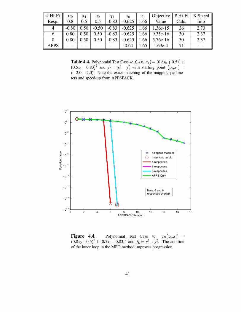
4.1.4 Polynomial Test 4: α - γ * O + 1 , ; β . 1

For polynomial test case 4, the high fidelity function takes the exact form

fHx0 x1

0 8x0 0 5 2 0 5x1 0 83 2

The results of the multifidelity optimization calculation are displayed in Table 4.4 andFigure 4.4. The results show that the space mapping parameters are nearly an exact matchregardless of the number of high fidelity responses used by the inner loop. There is a sign

36

difference in some of the mapping parameters, but this is still a match since the terms aresquared for use in the algorithm. A beneficial speed-up over traditional APPSPACK is alsoevident.

4.1.5 Polynomial Test 5: α * O + 10 ,$- γ * O + 100 , ; β . 1

The high fidelity function with the exact form

fHx0 x1

8 0x0 50 0 2 5 0x1 83 0 2

is used in polynomial test case 5. The comparison between the APPSPACK and MFOresults are shown in Table 4.5 and Figure 4.5. As was the case for the previous tests, thespace mapping parameters are nearly an exact match for all the cases and scale well withthe polynomial test case 1. Although there is a sign difference for some of the mappingparameters, the terms are squared when used so this can still be considered a match.

4.1.6 Polynomial Test 6: α * O + 100 ,/- γ * O + 10000 , ; β . 1

For the final polynomial test, the high fidelity function has the exact form

fHx0 x1

80 0x0 5000 0 2 50 0x1 8300 0 2

Table 4.6 and Figure 4.6 display the results obtained using both the MFO and the traditionalAPPSPACK algorithms. The space mapping parameters are nearly an exact match and asignificant speed-up is observed.

37

# Hi-Fi γ0 γ1 x0 x1 Objective # Hi-Fi X SpeedResp. 0.5 -0.83 -0.5 0.83 Value Calc. Imp

2 0.50 -0.83 -0.499 0.835 2.86e-5 21 2.764 0.50 -0.83 -0.50 0.83 1.0e-20 25 2.326 0.50 -0.83 -0.50 0.83 2.0e-20 28 2.078 0.50 -0.83 -0.50 0.83 4.0e-20 32 1.81

APPS — — -0.50 0.85 4.0e-4 58 —

Table 4.1. Polynomial test case 1: fH x0 x1 10 x0 2 0 3 5 2 2 x1 4 0 3 83 2 and fL 0 y20 2 y2

1 with starting point x0 x1 50 4 2 3 0 64 2 3 0 . Note the exact matching of the mapping parame-ters.

0 2 4 6 8 10 12 1410−20

10−15

10−10

10−5

100

105

APPSPACK Iteration

Func

tion

Val

ue

no space mapping

inner loop result

2 responses

4 responses

6 responses

8 responses

APPS Only

Figure 4.1. Polynomial Test Case 1: fH x0 x1 70 x0 2 0 3 5 2 2 x1 4 0 3 83 2 and fL 0 y20 2 y2

1. In searching for a minimum offH the MFO algorithm progresses much quicker than traditionalAPPSPACK.

38


2 5.0 -8.3 -5.0 8.3 1.3e-17 21 2.764 5.0 -8.3 -5.0 8.3 1.0e-18 25 2.326 5.0 -8.3 -5.0 8.3 1.7e-17 28 2.078 5.0 -8.3 -5.0 8.3 0.0 32 1.81

APPS — — -5.0 8.5 4.0e-2 58 —

Table 4.2. Polynomial Test Case 2: fH x0 x1 80 x0 2 5 3 0 2 2 x1 4 8 3 3 2 and fL 0 y20 2 y2

1 with starting point x0 x1 90 4 20 3 0 64 20 3 0 . Note the exact matching of the mapping parame-ters and the nearly identical scaling to polynomial test case 1.

0 2 4 6 8 10 12 140

200

400

600

800

1000

1200

APPSPACK Iteration

Func

tion

Val

ue

no space mapping

inner loop result

2 responses

4 responses

6 responses

8 responses

APPS Only


1. The MFO method provides improvedalgorithm progression and results. Note that this is a linear plotsince the “8 response” case is exactly 0.

39


2 50.0 -83.0 -50.0 82.7 6.74e-2 21 2.764 50.0 -83.0 -50.0 83.0 1.0e-16 25 2.326 50.0 -83.0 -50.0 83.0 0.0 28 2.078 50.0 -83.0 -50.0 83.0 0.0 32 1.81

APPS — — -50.0 85.0 4.0e-2 58 —

Table 4.3. Polynomial Test Case 3: fH x0 x1 :0 x0 2 50 3 0 2 2 x1 4 83 3 0 2 and fL 0 y20 2 y2

1 with starting point x0 x1 50 4 200 3 0 64 200 3 0 . Note the exact matching of the mapping pa-rameters and the nearly identical scaling to polynomial test cases1 and 2.

0 2 4 6 8 10 12 140

2

4

6

8

10

12x 104

APPSPACK Iteration

Func

tion

Val

ue

no space mapping

inner loop result

2 responses

4 responses

6 responses

8 responses

APPS Only

Note: 6 and 8responses goesto exactly zero


1. The minimum obtained by the MFOmethod is better than the one found by traditional APPSPACK.Note that this is a linear plot since the “6 response” and “8 re-sponses” cases is exactly 0.

40

# Hi-Fi α0 α1 γ0 γ1 x0 x1 Objective # Hi-Fi X SpeedResp. 0.8 0.5 0.5 -0.83 -0.625 1.66 Value Calc. Imp

4 -0.80 0.50 -0.50 -0.83 -0.625 1.66 1.36e-15 26 2.736 0.80 0.50 0.50 -0.83 -0.625 1.66 9.35e-16 30 2.378 0.80 0.50 0.50 -0.83 -0.625 1.66 5.76e-16 30 2.37

APPS — — — — -0.64 1.65 1.69e-4 71 —

Table 4.4. Polynomial Test Case 4: fH x0 x1 ;0 0 3 8x0 2 0 3 5 2 2 0 3 5x1 4 0 3 83 2 and fL 0 y20 2 y2

1 with starting point x0 x1 <0 4 2 3 0 64 2 3 0 . Note the exact matching of the mapping parame-ters and speed-up from APPSPACK.

0 2 4 6 8 10 12 14 16 1810−16

10−14

10−12

10−10

10−8

10−6

10−4

10−2

100

102

APPSPACK Iteration

Func

tion

Val

ue no space mapping

inner loop result

4 responses

6 responses

8 responses

APPS Only

Note: 6 and 8responses overlap

Figure 4.4. Polynomial Test Case 4: fH x0 x1 =0 0 3 8x0 2 0 3 5 2 2 0 3 5x1 4 0 3 83 2 and fL 0 y20 2 y2

1. The additionof the inner loop in the MFO method improves progression.

41


4 -8.0 5.0 -50.0 -83.0 -6.25 16.6 4.06e-14 26 2.696 -8.0 5.0 -50.0 -83.0 -6.25 16.6 6.4e-17 30 2.338 8.0 5.0 50.0 -83.0 -6.25 16.6 4.1e-15 30 2.33

APPS — — — — -6.4 16.5 1.69 70 —

Table 4.5. Polynomial Test Case 5: fH x0 x1 >0 8 3 0x0 2 50 3 0 2 2 5 3 0x1 4 83 3 0 2 and fL 0 y20 2 y2

1 with startingpoint x0 x1 :0 4 20 3 0 64 20 3 0 . Note the exact matching of themapping parameters and the scaling with the polynomial in testcase 1.

0 2 4 6 8 10 12 14 16 1810−20

10−15

10−10

10−5

100

105

APPSPACK Iteration

Func

tion

Val

ue no space mapping

inner loop result

4 responses

6 responses

8 responses

APPS Only


1. Note the im-provement of MFO over APPSPACK.

42


4 80.0 50.0 5000.0 -8300.0 -62.5 166.0 2.81e-10 26 2.696 80.0 50.0 5000.0 -8300.0 -62.5 166.0 3.14e-11 30 2.338 80.0 50.0 5000.0 -8300.0 -62.5 166.0 3.08e-11 30 2.33

APPS — - — — -6.4 16.5 1.69e+4 70 —

Table 4.6. Polynomial Test Case 6: fH x0 x1 >0 80 3 0x0 2 5000 3 0 2 2 50 3 0x1 4 8300 3 0 2 and fL 0 y20 2 y2

1with starting point x0 x1 50 4 200 3 0 64 200 3 0 . The spacemapping parameters are almost an exact match.

0 2 4 6 8 10 12 14 16 1810−15

10−10

10−5

100

105

1010

APPSPACK Iteration

Func

tion

Val

ue no space mapping

inner loop result

4 responses

6 responses

8 responses

APPS Only

Note: 6 and 8responses overlap


1. Thespeed-up of the MFO algorithm over APPSPACK is about 2 times.

43

4.2 Multi-Variable Rosenbrock Function

In testing optimization methods, it is common to study the feasibility of an algorithm onthe Rosenbrock function. The function is

fR 100 ? y1 y20 @ 2

1 y0 2 (4.6)

and has a minimum at fR1 1 A 0 0. The multi-variable Rosenbrock function has N design

variables and can be written as

fMV Rx0 !!! xN B 1 N B 1

∑k 1 C 100 ? xk x2

k B 1 @ 2 1 xk B 1 2 D (4.7)

where fMVR1 !!!E 1 8 0 0 is a minimum. Note that (4.7) for N 2 is merely (4.6). Thus,

the Rosenbrock equation can be used as a low fidelity model and the multi-variable Rosen-brock as a corresponding high fidelity model. We examine these models to study the feasi-bility of mapping between models with different numbers of design variables.

To map between models with different numbers of design variables, a general mappingwas developed that captures the cross-dependencies of mapping parameters. This generalmapping has the following form

P F n G A F m H n G x F n GH Γ F m G (4.8)

where

A F m H n G IJK α00 !!! α0n... . . . ...

αm0 !!! αmn

LNMO Γ F m G IJK γ0...

γm

LNMO (4.9)

m is the number of low fidelity variables, and n is the number of high fidelity variables.The general mapping (4.8) can be reduced to our previous mapping, m n, by using onlythe diagonal terms of A F m H n G . Note that when the cross terms are required, additional highfidelity response calculations are required.

The following test cases were analyzed using the standard Rosenbrock function as thelow fidelity model and the multi-variable Rosenbrock as the high fidelity model:

Test 1: N 3, α00 E αmn O

1 , γ0 γm 0


1 , γ0 γm 0

44


1 , γ0 γm

O1

As with the polynomial test cases, the results from each test case are included in the nextsections in both table and graph formats. The tables contain basically the same informationas previously. One change is that the first column is now the the number of non-zero spacemapping parameters, from matrix (4.9), used in the calculations (# SM parameters). Thelast row of the table (APPS) still displays results obtained when APPSPACK was appliedto the high fidelity model (e.g. no calls to the inner loop). The other columns in the tableinclude the final values of the design variables (x0 !!!E xN), the final objective function value(Objective Value), the total number of high fidelity response calculations completed (# Hi-Fi Resp.), and the speed improvement of the MFO algorithm from traditional APPSPACK(X Speed Imp).

As before, the graph illustrates the algorithmic progression of each row in the table. Thex-axis indicates the number of successful APPSPACK iterations where successful refers toidentifying of a new best point. The y-axis shows the value of the objective function. Thelegend indicates which color corresponds to what number of non-zero high fidelity spacemapping parameters were used. The circles and stars indicate whether or not an inner loopcalculation was done to obtain the point respectively.

4.2.1 Multi-Variable Rosenbrock Test 1: N . 3, α00 -QPRPRPS- αmn * O + 1 , ,γ0 -QPRPRPS- γm . 0

This test uses the high fidelity function of the exact form

fHx0 x1 x2 8 100 ? x1 x2

0 @ 2 1 x0 2 100 ? x2 x2

1 @ 2 1 x1 2 (4.10)

and the exact mapping terms

A F 2 H 3 G UT α00 α01 α02α10 α11 α12 V Γ F 2 G WT 0

0 V (4.11)

In Table 4.7, results given the following testing conditions are displayed: 3 non-zero space mapping parameters; α10 α01 α02 0 0 4 non-zero space mapping parameters; α10 α01 0 0 6 non-zero space mapping parameters; all α are non-zero

Since the multi-variable Rosenbrock is a sum of squares whose minimum is 0, the equationcan be solved by setting each individual squared term equal to zero. Then, (4.10) shows

45

that x0 and x1 are forced to their optimum with the1 x0 2 and

1 x1 2 respectively.

Therefore x2 is only dependent on the x1 term via ? x2 x21 @ 2, and the only relevant cross

term is α12. Basically, the closer the problem is to the objective function the “non-relevant”space mapping parameters will go to zero.

Both Table 4.7 and Figure 4.7 show that a solution is found the quickest in the the caseof using three space mapping parameters. However, if four space mapping parameters areused, the speed-up is still significant and a better solution can be obtained.

4.2.2 Multi-Variable Rosenbrock Test 2: N . 4, α00 -QPRPRPS- αmn * O + 1 , ,γ0 -QPRPRPS- γm . 0

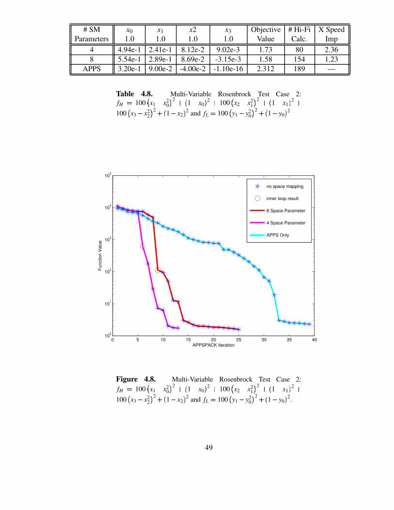
In test 2, the high fidelity function has the exact form

fHx0 x1 x2 8 100 ? x1 x2

0 @ 2 1 x0 2 100 ? x2 x2

1 @ 2 1 x1 2 100 ? x3 x2

2 @ 2 1 x2 2 (4.12)

and the exact mapping terms

A F 2 H 3 G T α00 α01 α02 α03α10 α11 α12 α13 V Γ F 2 G T 0

0 V (4.13)

Table 4.8 includes results for the following testing conditions: 4 non-zero space mapping parameters; α10 α01 α02 α03 0 0 8 non-zero space mapping parameters; all α are non-zero

As illustrated in Table 4.8 and Figure 4.8, the case with four non-zero space mappingparameters gives the best answer with the least amount of computational effort.

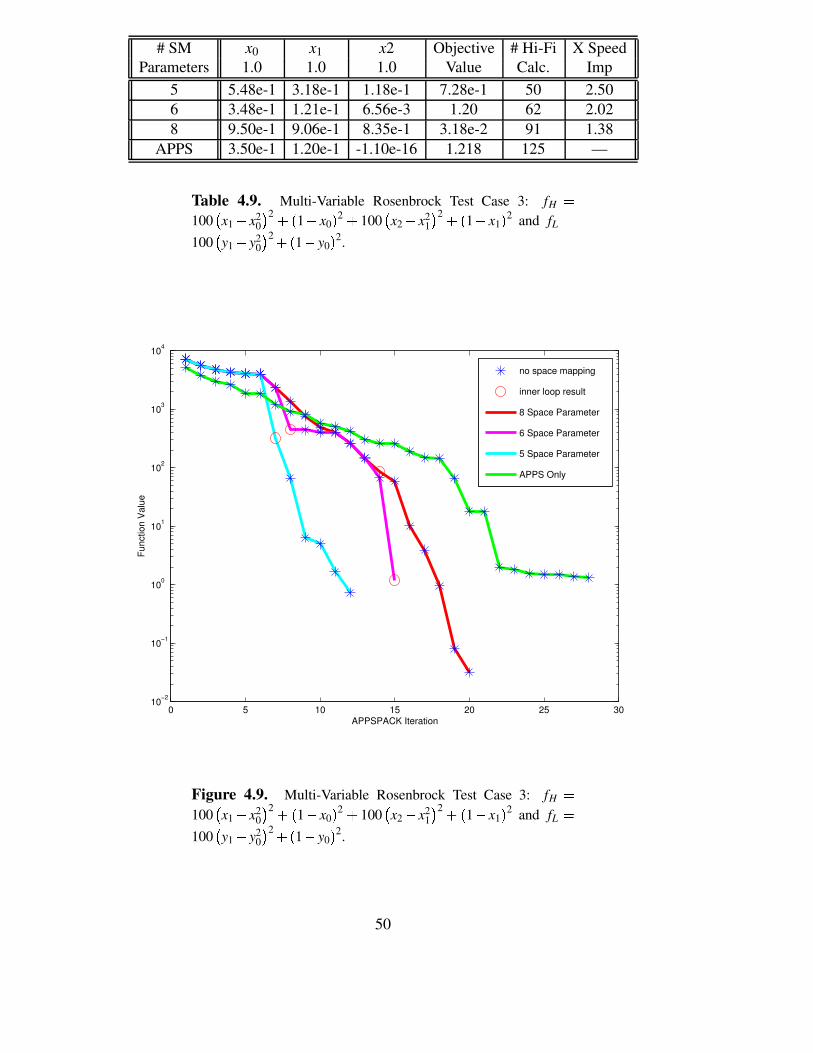
4.2.3 Multi-Variable Rosenbrock Test 3: N . 3, α00 -QPRPRPS- αmn * O + 1 , ,γ0 -QPRPRPS- γm * O + 1 ,

The exact form high fidelity function used in test 3 is

fHx0 x1 x2 8 100 ? x1 x2

0 @ 2 1 x0 2 100 ? x2 x2

1 @ 2 1 x1 2 (4.14)

46

and the exact mapping terms are

A F 2 H 3 G T α00 α01 α02α10 α11 α12 V Γ F 2 G T γ0

γ1 V (4.15)

Table 4.9 giving results for the following test conditions: 5 space parameters - α10 α01 α02 0 0 and all γ are non-zero 6 space parameters - α10 α01 0 0 and all γ are non-zero 8 space parameters - all α and γ are non-zero

The results are illustrated in Figure 4.9. The test condition with eight non-zero spacemapping parameters gives a significantly better solution. It requires more computationalwork than the other MFO runs, but it still provides some improvement over traditionalAPPSPACK.

47

# SM x0 x1 x2 Objective # Hi-Fi X SpeedParameters 1.0 1.0 1.0 Value Calc. Imp

3 7.29e-1 5.45e-1 2.93e-1 3.04e-1 42 2.984 8.29e-1 6.80e-1 4.57e-1 1.39e-1 50 2.506 2.99e-1 6.8e-1 4.57e-1 1.35 87 1.44

APPS 3.50e-1 1.20e-1 -1.10e-16 1.218 125 —

Table 4.7. Multi-Variable Rosenbrock Test Case 1: fH 0100 X x1 4 x2

0 Y 2 2 1 4 x0 2 2 100 X x2 4 x21 Y 2 2 1 4 x1 2 and fL 0

100 X y1 4 y20 Y 2 2 1 4 y0 2.

0 5 10 15 20 25 3010−1

100

101

102

103

104

APPSPACK Iteration

Func

tion

Val

ue

no space mappinginner loop result3 Space Parameter4 Space Parameter6 Space ParameterAPPS Only

Figure 4.7. Multi-Variable Rosenbrock Test Case 1: fH 0100 X x1 4 x2

0 Y 2 2 1 4 x0 2 2 100 X x2 4 x21 Y 2 2 1 4 x1 2 and fL 0

100 X y1 4 y20 Y 2 2 1 4 y0 2.

48

# SM x0 x1 x2 x3 Objective # Hi-Fi X SpeedParameters 1.0 1.0 1.0 1.0 Value Calc. Imp

4 4.94e-1 2.41e-1 8.12e-2 9.02e-3 1.73 80 2.368 5.54e-1 2.89e-1 8.69e-2 -3.15e-3 1.58 154 1.23

APPS 3.20e-1 9.00e-2 -4.00e-2 -1.10e-16 2.312 189 —

Table 4.8. Multi-Variable Rosenbrock Test Case 2:fH 0 100 X x1 4 x2

0 Y 2 2 1 4 x0 2 2 100 X x2 4 x21 Y 2 2 1 4 x1 2 2

100 X x3 4 x22 Y 2 2 1 4 x2 2 and fL 0 100 X y1 4 y2

0 Y 2 2 1 4 y0 2

0 5 10 15 20 25 30 35 40100

101

102

103

104

105

APPSPACK Iteration

Func

tion

Val

ue

no space mapping

inner loop result

8 Space Parameter

4 Space Parameter

APPS Only

Figure 4.8. Multi-Variable Rosenbrock Test Case 2:fH 0 100 X x1 4 x2

0 Y 2 2 1 4 x0 2 2 100 X x2 4 x21 Y 2 2 1 4 x1 2 2

100 X x3 4 x22 Y 2 2 1 4 x2 2 and fL 0 100 X y1 4 y2

0 Y 2 2 1 4 y0 2.

49

# SM x0 x1 x2 Objective # Hi-Fi X SpeedParameters 1.0 1.0 1.0 Value Calc. Imp

5 5.48e-1 3.18e-1 1.18e-1 7.28e-1 50 2.506 3.48e-1 1.21e-1 6.56e-3 1.20 62 2.028 9.50e-1 9.06e-1 8.35e-1 3.18e-2 91 1.38

APPS 3.50e-1 1.20e-1 -1.10e-16 1.218 125 —

Table 4.9. Multi-Variable Rosenbrock Test Case 3: fH 0100 X x1 4 x2

0 Y 2 2 1 4 x0 2 2 100 X x2 4 x21 Y 2 2 1 4 x1 2 and fL 0

100 X y1 4 y20 Y 2 2 1 4 y0 2.

0 5 10 15 20 25 3010−2

10−1

100

101

102

103

104

APPSPACK Iteration

Func

tion

Val

ue

no space mapping

inner loop result

8 Space Parameter

6 Space Parameter

5 Space Parameter

APPS Only

Figure 4.9. Multi-Variable Rosenbrock Test Case 3: fH 0100 X x1 4 x2

0 Y 2 2 1 4 x0 2 2 100 X x2 4 x21 Y 2 2 1 4 x1 2 and fL 0

100 X y1 4 y20 Y 2 2 1 4 y0 2.

50

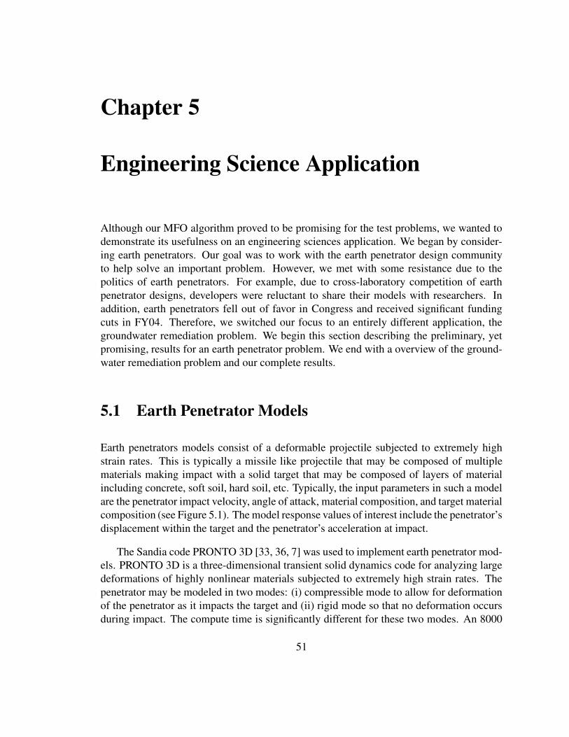
Chapter 5

Engineering Science Application

Although our MFO algorithm proved to be promising for the test problems, we wanted todemonstrate its usefulness on an engineering sciences application. We began by consider-ing earth penetrators. Our goal was to work with the earth penetrator design communityto help solve an important problem. However, we met with some resistance due to thepolitics of earth penetrators. For example, due to cross-laboratory competition of earthpenetrator designs, developers were reluctant to share their models with researchers. Inaddition, earth penetrators fell out of favor in Congress and received significant fundingcuts in FY04. Therefore, we switched our focus to an entirely different application, thegroundwater remediation problem. We begin this section describing the preliminary, yetpromising, results for an earth penetrator problem. We end with a overview of the ground-water remediation problem and our complete results.

5.1 Earth Penetrator Models

Earth penetrators models consist of a deformable projectile subjected to extremely highstrain rates. This is typically a missile like projectile that may be composed of multiplematerials making impact with a solid target that may be composed of layers of materialincluding concrete, soft soil, hard soil, etc. Typically, the input parameters in such a modelare the penetrator impact velocity, angle of attack, material composition, and target materialcomposition (see Figure 5.1). The model response values of interest include the penetrator’sdisplacement within the target and the penetrator’s acceleration at impact.

The Sandia code PRONTO 3D [33, 36, 7] was used to implement earth penetrator mod-els. PRONTO 3D is a three-dimensional transient solid dynamics code for analyzing largedeformations of highly nonlinear materials subjected to extremely high strain rates. Thepenetrator may be modeled in two modes: (i) compressible mode to allow for deformationof the penetrator as it impacts the target and (ii) rigid mode so that no deformation occursduring impact. The compute time is significantly different for these two modes. An 8000

51

V

!

"p

"c

"N

Target-y

Figure 5.1. Simple graphic depicting an earth penetrator com-posed of multiple materials (depicted by density ρ) striking a tar-get.

element mesh in the compressible mode takes approximately 40 minutes to execute whilethe rigid mode takes only about 10 seconds on the same computer, a computational ratioof 1:240. A parameter study varying the penetrator density and corresponding accelerationresponse is shown in Figure 5.2. The elastic body results in an oscillatory acceleration re-sponse since the body is compressible and pressure waves within the body produce thesenoisy oscillations. In contrast, the rigid body has a relatively smooth acceleration responsewith respect to density, but it captures the trend of the elastic body. This factor and thedifference in compute times make this problem an ideal candidate for multifidelity opti-mization.

Many different earth penetrator calculations were done minimizing acceleration andmaximizing displacement by varying penetrator density. With these calculations, a 2-3times speed up was observed with displacement and 1-2 times speed was observed withacceleration. One case of particular interest is shown in Figure 5.3 and Table 5.1. Theacceleration of the penetrator was minimized such that high fidelity model = elastic model with fine mesh (see Figure 5.2) , low fidelity model = rigid model with fine mesh.

As Figure 5.3 illustrates, the MFO approach actually takes longer, but finds an improved

52

Parameter Study - Acceleration dependence on Density

0.00E+00

2.00E+07

4.00E+07

6.00E+07

8.00E+07

1.00E+08

1.20E+08

1.40E+08

1.60E+08

1.80E+08

2.00E+08

0 0.5 1 1.5 2 2.5 3 3.5 4 4.5

Density

Acceleration

acceleration - coarse (elastic)

acceleration-fine (rigid)

acceleration-fine (elastic)

CoarseCoarse

MeshMeshFineFine

MeshMesh

18018024002400ElasticElastic

Calc. TimeCalc. Time

(s)(s)

1152115278487848# Elements# Elements

Figure 5.2. Parameter study of acceleration response of earthpenetrator with varying density impacting a concrete target. Notehow the rigid penetrator captures the trend of the elastic penetratorwithout the ”noise”.

minimum. The reason for this is that traditional APPSPACK becomes trapped at a localminimum. Since the acceleration response of the rigid body is smooth and captures thecorrect trend, it pushes the optimization past the local noise and finds the a better minimum(see Figure 5.4). This result is in no way implying that our MFO algorithm guarantees aglobal minimum, just that the behavior was observed in this specific case.

53

1 1.5 2 2.5 3 3.5 4 4.5 55

5.5

6

6.5

7

7.5

8

8.5

9x 107

APPSPACK Iteration

Func

tion

Val

ue

no space mappinginner loop resultAPPS OnlyInner Loop Calculation

Figure 5.3. Comparison of traditional APPSPACK and MFO(specified as Inner Loop Calculation) on the problem of mini-mizing the acceleration of an earth penetrator. See Table 5.1 forspecifics. Although the MFO case takes longer to optimize, it findsthe “observed” optimum (see Figure 5.4).

Optimization Objective # Hi-Fi X SpeedScheme Value Calc. ImpMFO 5.0e7 11 0.82APPS 7.3e7 9 —

Table 5.1. Comparison of traditional APPSPACK and MFO onthe problem of minimizing acceleration of an earth penetrator. Al-though the MFO case takes longer to optimize, it finds a betteroptimum (see Figure 5.4).

54

Parameter Study - Acceleration dependence on Density

0.00E+00

2.00E+07

4.00E+07

6.00E+07

8.00E+07

1.00E+08

1.20E+08

1.40E+08

1.60E+08

1.80E+08

2.00E+08

0 0.5 1 1.5 2 2.5 3 3.5 4 4.5

Density (*6.e-4)

Acceleration

acceleration-fine (elastic)

observed optimum

found optimum

Figure 5.4. Traditional APPSPACK calculates the local optimumspecified with the red arrow. The MFO scheme demonstrates aglobal search capability and finds a better optimum at the purplearrow. From the parameter study this is the observed optimum, butnot necessarily the global optimum.

55

5.2 Groundwater Remediation Models

Remediation is a technique that is employed to reduce or minimize the negative health andenvironmental impacts of chemical contamination. One method of groundwater remedi-ation, hydraulic capture (HC), uses the design of a well field to alter the direction of thegroundwater flow and reverse or halt the migration of the contaminant plume. For exam-ple, a well field can be designed so that gradients point toward the interior of the plume,resulting in containment and possible shrinkage of the plume. The overall goal of HC is tocontain or shrink a plume at minimum cost. Therefore, optimization is a useful tool for thedesign of an appropriate well field.

Plume migration control is an active area of research in environmental engineering.The three prime areas of focus are: improving models of subsurface flow and transport,incorporating installation and operational costs of HC into the objective functions, anddeveloping and calibrating capture constraints so that computational efficiency is obtainedin the modeling process while simultaneously avoiding excessive pumping in the final welldesign. Once an objective function and constraints are developed, optimization techniquesare used to determine the well design that minimizes the remediation cost while satisfyingthe constraints. Mathematically, these problems are challenging because evaluation of theobjective function and constraints typically requires the results of a simulation. This meansthat necessary gradient information may be difficult or impossible to obtain.

The problem studied here is motivated by a hydraulic capture application proposedas part of a suite of benchmarking test problems in [27]. This entire test suite of prob-lems includes data for several different physical domains and objective functions as well asguidelines for comparison. For the HC application, it is left to the modeler to choose thecapture constraint and the concentration contour of the plume boundary.

5.2.1 Models of Hydraulic Capture

In this study, we consider two hydraulic capture models: transport-based concentrationcontrol (TBCC) and flow-based hydraulic control (FBHC). For both models, the optimiza-tion problem is

minu Z Ω

Ju (5.1)

where u is a vector of decision variables and Ω is the feasible region of u and can berepresented by a set of constraint equations.

56

The objective function J is merely the sum of the capital (or installation) cost Jc andthe operational cost Jo and can be stated as follows [27, 26]:

J n

∑i 1

c0db0i ∑

Qi [ 0 \ 0 c1 Qmi b1

zgs hmin b2] ^`_ a

Jc b t f

0 c ∑i HQi [ 0 \ 0 c2Qi

hi zgs ∑

i HQi d 0 \ 0 c3Qi e dt] ^`_ aJo

(5.2)

In Jc the first term accounts for drilling and installing all the wells and the second termrepresents the additional cost for pumps for extraction wells. In Jo the term pertaining theextraction wells includes the lift cost associated with raising the water to the surface. Morespecifically, in (5.2) c j and b j are cost coefficients and exponents, respectively, di zgs isthe depth of well i Qm

i is the design pumping rate, and hmin is the minimum allowable head.We use the values hmin 10

m and Qm

i gf 0 0064m3 h s and di 30

m for each pump

i. Note that a negative pumping rate means a well is extracting and a positive pumping ratesmeans a well is injecting and that injection wells are assumed to operate under gravity feedconditions. The simulation time is t f 5 years. Other pertinent cost data is given in [26].

The number of wells, n i N and pumping rates j Qi k ni 1 are decision variables. If, in

the course of the optimization, a well rate satisfies the inequality Qi li 10 B 6 m3 h s , thatwell is removed from the design space and excluded from all other calculations. Althoughthis restriction leads to a discontinuous objective function, the benefit is a decrease in theinstallation cost and a well design with fewer wells operating at higher rates. We assumethat all wells have a fixed depth, but that their location can vary in the x y plane. Thesewell locations, j xi yi k n

i 1 are also decision variables, but do not explicitly appear in theobjective function.

The hydraulic heads, him for well i, also vary with the decision variables and obtain-

ing their values at each iteration requires a solution to equations that model saturated flow.The model is given by

Ss∂h∂t

∇ ! K ! ∇h S (5.3)

where Ss1 h m is the specific storage coefficient, h

m is the hydraulic head, K

m h s is the

hydraulic conductivity tensor, and Sm3 h s is a fluid source term and is where the decision

variables enter into the state equation for the HC problem. Numerically, the simulatorMODFLOW2000 [38] is used to find a solution to (5.3).

In HC models, constraints on the decision variables typically include bounds on thewell capacities and the hydraulic head at each well location. For example, we incorporate

57

the inequalities

Qemax i Qi i Qimax m3 h s i 1 mnm n (5.4)

hmax # hi # hmin m ) i 1 mmn n (5.5)

where, Qemax is the maximum extraction rate at any well, Qimax is the maximum injectionrate at any well, hmax is the maximum allowable head, and hmin is the minimum allowablehead. Note that assessing whether or not (5.5) holds requires a solution to (5.3). In additionto (5.4) and (5.5), the HC problem constrains the net pumping rate using the inequality

QT n

∑i 1

Qi # QmaxT (5.6)

where QmaxT

m3 h s is the maximum allowable total extraction rate. This ensures that the

land is not completely drained of all its water resources.

5.2.1.1 Flow-based Hydraulic Control (FBHC)

Flow-based hydraulic control is a technique for plume containment that enforces head gra-dient constraints around the perimeter of the plume. In the particular model we consider,a head gradient constraint is formulated as a constraint on the difference in hydraulic headvalues at specified locations. Consider

hk1 hk

2 # dm ) k 1 M (5.7)

where M is the number of head gradient constraints imposed around the boundary, h1 h2are hydraulic head values at specified nodes for each constraint k, and d is the bound onthe difference. This set of constraints can be used to enforce head gradients vertically orhorizontally. For example, in the simple case where h1 are h2 are aligned at a distance ofdistance ∆x apart, then dividing (5.7) by ∆x yieldso

hk1 hk

2∆x p # d

∆xm h s (5.8)

The FBHC approach to the HC problem is minimizing the objective function J subjectto (5.4), (5.5), (5.6) and (5.7). Use of this method is attractive because it is relativelyinexpensive. However, it requires (5.7) to be calibrated to ensure that the contaminantplume is properly captured and to avoid excessive pumping [28].

58

5.2.1.2 Transport Based Concentration Control (TBCC)

A direct approach for plume containment is to impose constraints on the concentration atspecified locations. This constraint can be expressed as

C j i Cmaxj

kg h m3 (5.9)

where C j is the concentration at some observation node j and Cmaxj is the maximum al-

lowable concentration. Evaluation of this constraint requires a solution to the contaminanttransport equation

∂θαCι ∂t

∇ ! θαDι ! ∇Cι ∇ ! qCι Iι Rι Sι (5.10)

where Cι kg h m3 is the concentration of species ι in the aqueous phase, θα is the volumefraction of the aqueous phase, D is a hydrodynamic dispersion tensor, v

m h s is the mean

pore velocity, qm h s is the Darcy velocity, and I ι Rι Sι represent interphase mass transfer,

biogeochemical reactions, and source of mass respectively. Numerically, the simulatorknown as MT3DMS [39] is used to obtain a solution to the transport equation.

Solving the HC problem using the TBCC model is minimizing the cost function J withrespect to (5.4), (5.5), (5.6), and (5.9). Therefore, the TBCC approach requires a solution toboth (5.10) and (5.3) making it computationally expensive. Moreover, objective functionsand constraints involving concentrations are nonconvex in some situations [6, 3], makingthe minimization problem more difficult.

5.2.2 HC Problem for Comparison

In the MFO approach to the HC problem, we use the FBHC model as the low fidelitymodel and the TBCC model as the corresponding high fidelity model. In order to test theeffectiveness of the MFO approach, we compare results for the HC problem included in theset of community problems proposed in [27]. For the simple domain of this problem, theFBHC formulation has been shown to be sufficient [12]. However, it should be noted thatother approaches are needed for more realistic domains [1].

In the HC problem used here, the physical domain is a 1000 q 1000 q 30m unconfined

aquifer. Since the aquifer is unconfined, the head constraint (5.5), depends nonlinearly onthe pumping rates. For the hydraulic conductivity field, we use the simple homogeneouscase with K 5 01 q 10 B 5 m h s Paired with the saturated flow equation (5.3), we use thefollowing boundary and initial conditions:

∂h∂x rrrr x 0

∂h∂y rrrr y 0

∂h∂z rrrr z 0

0 t 0

59

qzx y z h t 0 8s 1 903x10 B 8 m h s where qz s K

∂h∂z

h1000 y z t 0 20 0 001y

m

hx 1000 z t 0 1 20 0 001x

m

Here qz is the Darcy flux out of the domain, representing recharge into the aquifer thatcould result from rainfall. The steady state solution to the flow problem without wellsis h

x y z 0 t hs

m and Ss 2 0 q 10 B 1 1 h m is the specific yield of the unconfined

aquifer. The ground surface elevation is zgs 30m )

A plume development was simulated using (5.10) from a finite source for five yearswith a constant concentration of 1kg h m3 located in the region bounded by 200 225 ; 475 525 h h 2 m )We chose the 5 q 10 B 5 kg h m3 contour line as the plume boundary and set Cmax

j 5 q10 B 5 kg h m3 in (5.9). The MT3DMS [39] was used to generate this initial contaminantplume, as described in [26].

For the FBHC approach, we use five head difference constraints (5.7) with d 10 B 4 Five concentration constraints (5.9) are used for the TBCC approach, enforced in the samelocations as (5.7) in the FBHC approach. The starting point includes two extraction andtwo injection wells for a total of N 4 candidate wells and initial pumping rates of f Qi 0 0064

m3 h s .

5.2.3 Numerical Results

The financial cost of the remediation at the initial iterate is Ju0 u $78 587 Table 5.2

shows the minimum financial cost found and the %-decrease for each of the approaches–FBHC, TBCC, and MFO. Both the FBHC and TBCC models were solved using APPSPACK4.0, the same software customized for the APPS/Space Mapping approach to MFO. Notethat all three methods produce solutions with similar remediations costs and overall per-centage decreases.

One way to view the computational performance of the algorithms is to consider thenumber of function evaluations needed to reach the optimal point. As with most simulation-based optimization problems, the majority of the computational cost in the function eval-uation is the calls to the MODFLOW2000 and/or MT3DMS simulators. Note that if (5.6)is not satisfied, a flow simulation is not performed in any approach and likewise if (5.5) isnot satisfied, then no transport simulation is performed for the TBCC or MFO approaches.The fourth and fifth columns in Table 5.2 show the number of times that MODFLOW2000(mf2k) and MT3DMS (mt3d) were called for each approach. For this problem, a MOD-FLOW2000 simulation takes approximately 2 seconds, wall clock time and a MT3DMSsimulation takes anywhere from 40 to 50 seconds wall clock time.

60

Figure 5.5 highlights the differences in the three approaches by illustrating their per-formances over the course of the algorithm’s execution. All three approaches start off thesame. However, once the MFO approach receives the results of an inner loop calculation,it is able to make a significant decrease in the overall cost more quickly.

5.2.4 Discussion

In [27], many of the existing challenges in optimal design of problems involving saturatedflow and transport are addressed. The lack of representative problems to be used for thetesting and comparison of methods is discussed, and a set of test problems is presented.Although the test problems were developed after an extensive literature search and areindicative of real world problems, the domain is still relatively simple. For this simple, ho-mogeneous case considered in this work, the FBHC model is sufficient and computationallycost-effective [11]. However, the introduction of heterogeneities or other complexities willlikely require the TBCC or other models in which the plume boundary is precisely defined.Since this may not be a viable alternative with respect to computational cost, we offer theMFO approach. We have shown that the MFO approach is a comparable method and thusmay be a reasonable method for the solution of groundwater remediation problems. Tofurther investigate its usefulness in this case, we plan to extend our study to consider morerepresentative physical models and simulators and to incorporate real-site data.

61

Model Cost % Decrease mf2k calls mt3d callsFBHC $24,175 69.2% 117 0TBCC $20,362 74.1% 188 160MFO $22,428 71.5% 152 86

Table 5.2. Comparison of results from solving a groundwater re-mediation problem using three different models. The first columngives the model used in the problem statement while the remainingfour columns give the corresponding performance information.

1 2 3 4 5 6 7 8 9 102

3

4

5

6

7

8x 10

4

APPSPACK Iteration

Func

tion

Val

ue

TBCCFBHCMFO

Figure 5.5. Graph showing the reduction in the groundwater re-mediation cost function versus the number of APPSPACK itera-tions. The solid blue line and green dashed lines correspond to thesolutions of the TBCC and the FBHC models, respectively, solvedwith APPSPACK 4.0. The red dot-dash line corresponds to solv-ing the problem using the MFO approach. Note that the significantdecrease corresponding to the red dot (at iteration 4) was the resultof and inner loop calculation.

62

Chapter 6

Conclusions and Future Work

In this paper, we have described an approach to multifidelity optimization based on asyn-chronous parallel pattern search and space mapping. Two important features of our ap-proach are: (i) it is provably convergent and (ii) the number of design variables betweenmodels of differing fidelity may be non-equivalent in both number and type. Our MFOscheme was implemented using the existing APPSPACK software and a customized or-acle. This oracle is composed of a series of scripts that control the calculation of thespace mapped low fidelity optimization calculation. This report describes the implementa-tion details and illustrates our success for a set of test problems including polynomial andmulti-variable Rosenbrock and for two engineering science applications– earth penetratorsand groundwater remediation.

Throughout the course of this work, some topics of interest arose that we were unfortu-nately unable to touch upon. Future work in this area should consider them. For example,a more generic and dynamic mapping could be developed through the use of data mining.In this case, the selection of the space mapping terms would be based on both past andruntime calculations, and the space mapping formulation would be improved at each runof the application. Another approach might include 1st and 2nd order corrective modelsin the mapping terms as done in [29]. Note that this would require intermittent calls tofixed patterns in order to calculate the derivate terms, and therefore, a more generic oracleimplementation would be needed.

Currently, our MFO scheme is a set of standalone scripts that work in conjunctionwith APPSPACK. We believe it would be beneficial to incorporate our scheme into theDAKOTA toolkit. Future engineering science applications of our MFO algorithm includean extended set of groundwater problems that may contain a model of Long Island cur-rently being developed at SUNY-Buffalo. In addition, there are many relevant optimizationproblems for circuit and device model codes at Sandia.

63

References

[1] D. P. Ahfeld, R. Page, and G. F. Pinder. Optimal ground-water remediation methodsapplied to a superfund site: from formulation to implementation. Ground Water,33(1):58–70, 1995.

[2] D. P. Ahlfeld and M. Heidari. Applications of optimal hydraulic control to ground-water systems. J. of Water Resources Planning and Management, 120(3):350–365,1994.

[3] D. P. Ahlfeld and M. P. Sprong. Presence of nonconvexity in groundwater concentra-tion response functions. J. of Water Resources Planning and Management, 124(1):8–14, 1998.

[4] Mohamed H. Baker and John W. Bandler. An introduction to the space mappingtechnique. Optimization and Engineering, 2:369–384, 2001.

[5] John W. Bandler, Mostafa A. Ismail, Jose Ernesto Rayas-Sanchez, and Qi-Jun Zhang.Neuromodeling of microwave circuits exploiting space-mapping technology. IEEETransactions on Microwave Theory and Techniques, 47(12):2417–2427, 1999.

[6] A. Battermann, J.M. Gablonsky, A. Patrick, C.T. Kelley, and K.R. Kavanagh. Solutionof a groundwater flow problem with implicit filtering. Optimization and Engineering,3:189–199, 2002.

[7] Kevin H. Brown, J. Richard Koteras, Don B. Longcope, and Thomas L. Warren. Cav-ity expansion: A library for cavity expansion algorithms, version 1.0. Technical Re-port SAND2003-1048, Sandia National Laboratories, Albuquerque, NM 87185, April2003.

[8] J. E. Dennis, Jr. and V. Torczon. Direct search methods on parallel machines. SIAMJ. Opt., 1:448–474, 1991.

[9] E. D. Dolan, R. M. Lewis, and V. Torczon. On the local convergence properties ofparallel pattern search. Technical Report 2000-36, NASA Langley Research Center,Institute for Computer Applications in Science and Engineering, Hampton, VA, 2000.

[10] Michael S. Eldred, Laura P. Swiler, David M. Gay, Shannon L. Brown, Anthony A.Giunta, William E. Hart, and Jean-Paul Watson. DAKOTA: A multilevel parallel

64

object-oriented framework for design optimization, parameter estimation, uncertaintyquantification, and sensitivity analysis - version 3.3 reference manual. Technical Re-port SAND2001-3515, Sandia National Laboratories, Albuquerque, NM 87185, De-cember 2004.

[11] K.R. Fowler, C.T. Kelley, C.E. Kees, and C. T. Miller. A hydraulic capture applicationfor optimal remediation design. In C.T. Miller, M.W. Farthing, W.G. Gray, and G.F.Pinder, editors, Proceedings of the XV International Conference on ComputationalMethods in Water Resources, 2004.

[12] K.R. Fowler, C.T. Kelley, C.T. Miller, M. S. Reed, C.E. Kees, and R. W. Darwin. So-lution of a well field design problem with implicit filtering. to appear in Optimizationand Engineering, 2003.

[13] David M. Gay. Usage summary for selected optimization routines. Technical ReportComputing Science Technical Report No. 153, AT&T Bell Laboratories, Murray Hill,NJ 07974, October 1990.

[14] Anthony A. Giunta. Use of data sampling, surrogate models, and numerical optimiza-tion in engineering design. In Proceedings of 40th AIAA Aerospace Sciences Meetingand Exhibit, AIAA Paper 2002-0538, pages 1–13. AIAA, 2002.

[15] Genetha A. Gray and Tamara G. Kolda. APPSPACK 4.0: Asynchronous parallelpattern search for derivative-free optimization. Technical Report SAND2004-6391,Sandia National Laboratories, Livermore, CA 94551, August 2004.

[16] W. Gropp, E. Lusk, N. Doss, and A. Skjellum. A high-performance, portable imple-mentation of the MPI message passing interface standard. Parallel Comp., 22:789–828, 1996.

[17] W. D. Gropp and E. Lusk. User’s guide for mpich, a portable implementation of MPI.Technical Report ANL-96/6, Mathematics and Computer Science Division, ArgonneNational Laboratory, 1996.

[18] P. D. Hough, T. G. Kolda, and V. Torczon. Asynchrounous parallel pattern search fornonlinear optimization. SIAM J. Sci. Comput., 23:134–156, 2001.

[19] Tamara G. Kolda. Revisiting asynchronous parallel pattern search. Technical Re-port SAND2004-8055, Sandia National Laboratories, Livermore, CA 94551, Febru-ary 2004.

[20] Tamara G. Kolda, Robert Michael Lewis, and Virginia Torczon. Optimization by di-rect search: New perspectives on some classical and modern methods. SIAM Review,45(3):385–482, 2003.

[21] Tamara G. Kolda and Virginia J. Torczon. Understanding asynchronous parallel pat-tern search. In Gianni Di Pillo and Almerico Murli, editors, High Performance Algo-rithms and Software for Nonlinear Optimization, volume 82 of Applied Optimization,pages 316–335. Kluwer Academic Publishers, Boston, 2003.

65

[22] Tamara G. Kolda and Virginia J. Torczon. On the convergence of asynchronous par-allel pattern search. SIAM Journal on Optimization, 14(4):939–964, 2004.

[23] R. M. Lewis and V. Torczon. Rank ordering and positive bases in pattern search algo-rithms. Technical Report 96–71, Institute for Computer Applications in Science andEngineering, Mail Stop 132C, NASA Langley Research Center, Hampton, Virginia23681–2199, 1996.

[24] R. M. Lewis and V. Torczon. Rank ordering and positive basis in pattern searchalgorithms. Technical Report 96-71, NASA Langley Research Center, Institute forComputer Applications in Science and Engineering, Hampton, VA, 1996.

[25] Robert Michael Lewis, Virginia Torczon, and Michael W. Tross et. Direct searchmethods: Then and now. Journal of Computational and Applied Mathematics, 124(1–2):191–207, December 2000.

[26] A.S. Meyer, C.T. Kelley, and C.T. Miller. Electronic supplement to ”optimal designfor problems involving flow and transport in saturated porous media”. Advances inWater Resources, 12:1233–1256, 2002.

[27] A.S. Meyer, C.T. Kelley, and C.T. Miller. Optimal design for problems involving flowand transport in saturated porous media. Advances in Water Resources, 12:1233–1256, 2002.

[28] A. E. Mulligan and D. P. Ahlfeld. Advective control of groundwater contaminantplumes: Model development and comparison to hydraulic control. Water ResourcesResearch, 35(8):2285–2294, 1999.

[29] T. D. Robinson, M. S. Eldred, K. E. Wilcox, and R. Haimes. Strategies for multifi-delity optimization with variable dimensional hierarchical models. In abstract sub-mitted for 47th AIAA/ASME/ASCE/AHS/ASC Structures, Structural Dynamics, andMaterials Conference (2nd AIAA Multidisciplinary Design Optimization SpecialistConference), Newport, Rhode Island, May 1-4, 2006.

[30] H. H. Rosenbrock. An automatic method for finding the greatest and least value of afunction. Computer Journal, 3:175–184, 1960.

[31] Klaus Schittkowski. More test problems for nonlinear programming codes. LectureNotes in Economics and Mathematical Systems, 282:118–223, 1987.

[32] Gregory D. Sjaardema. APREPRO: An algebraic preprocessor for parameterizingfinite element analyses. Technical Report SAND92-2291, Sandia National Laborato-ries, Albuquerque, NM 87185, March 1997.

[33] L. M. Taylor and D. P. Flanagan. Pronto 3D a three-dimensional transient solid dy-namics program. Technical Report SAND87-1912, Sandia National Laboratories,Albuquerque, NM 87185, December 1992.

66

[34] V. Torczon. PDS: Direct search methods for unconstrained optimization on eithersequential or parallel machines. Technical Report TR92-09, Rice University, Depart-ment of Computational & Applied Math, Houston, TX, 1992.

[35] V. Torczon. On the convergence of pattern search algorithms. SIAM J. Opt., 7:1–25,1997.

[36] Thomas L. Warren and Mazen R. Tabbara. Spherical cavity-expansion forcing func-tion in pronto 3d for application to penetration problems. Technical Report SAND97-1174, Sandia National Laboratories, Albuquerque, NM 87185, May 1997.

[37] Margaret H. Wright. Direct search methods: Once scorned, now respectable. InD. F. Griffiths and G. A. Watson, editors, Numerical Analysis 1995 (Proceedings ofthe 1995 Dundee Biennial Conference in Numerical Analysis), volume 344 of PitmanResearch Notes in Mathematics, pages 191–208. CRC Press, 1996.

[38] C. Zheng, M. C. Hill, and P. A. Hsieh. MODFLOW2000, The U.S.G.S Survey ModularGround-Water Model User Guide to the LMT6 Package, the Linkage With MT3DMSfor Multispecies Mass Transport Modeling. USGS, user’s guide edition, 2001.

[39] C. Zheng and P. P. Wang. MT3DMS: A Modular Three-Dimensional MultispeciesTransport Model for Simulation of Advection, Dispersion, and Chemical Reactionsof Contaminants in Groundwater Systems, documentation and user’s guide edition,1999.

67

Appendix A

Inner Loop Scripts

Here, we give explicit examples of scripts written to carry out our MFO scheme. Thesescripts are included to elucidate some of difficult details found in this document. All scriptswere executed in a csh environment. Both PERL commands and Java calls to externalparsers (for generating the aprepro type files) were used. The following scripts and fileswere included in the top level directory structure: high fi script – calculates the high fidelity response. low fi script – calculates the low fidelity response. interface template script – placeholder for many of the default advanced user options

(changes made be expert users only). mfo script – primary multifidelity optimization script. RUN MFO SCRIPT – high level run script. USER INTERFACE SCRIPT – placeholder for options that are to be modified bythe user for each application. APPSPACK INPUT FILE – APPSPACK input file. response template.txt – m4 file used to extract the relevant response values. templatedir highfi – directory containing files required to complete a high fidelityfunction calculation.

– high fi input template.txt – file containing function input in aprepro format.

– ParseFileToAprepro.class – java parser file that creates many of the apreprofiles.

– application specific auxiliary files required for a high fidelity calculation; in-cludes simulators.

68

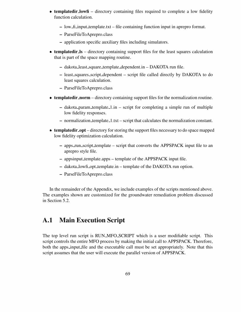
templatedir lowfi – directory containing files required to complete a low fidelityfunction calculation.

– low fi input template.txt – file containing function input in aprepro format.

– ParseFileToAprepro.class

– application specific auxiliary files including simulators. templatedir ls – directory containing support files for the least squares calculationthat is part of the space mapping routine.

– dakota least square template dependent.in – DAKOTA run file.

– least squares script dependent – script file called directly by DAKOTA to doleast squares calculation.

– ParseFileToAprepro.class templatedir norm – directory containing support files for the normalization routine.

– dakota param template 1.in – script for completing a simple run of multiplelow fidelity responses.

– normalization template 1.txt – script that calculates the normalization constant. templatedir opt – directory for storing the support files necessary to do space mappedlow fidelity optimization calculation.

– apps run script template – script that converts the APPSPACK input file to anaprepro style file.

– appsinput template.apps – template of the APPSPACK input file.

– dakota lowfi opt template.in – template of the DAKOTA run option.

– ParseFileToAprepro.class

In the remainder of the Appendix, we include examples of the scripts mentioned above.The examples shown are customized for the groundwater remediation problem discussedin Section 5.2.

A.1 Main Execution Script

The top level run script is RUN MFO SCRIPT which is a user modifiable script. Thisscript controls the entire MFO process by making the initial call to APPSPACK. Therefore,both the apps input file and the executable call must be set appropriately. Note that thisscript assumes that the user will execute the parallel version of APPSPACK.

69

BEGIN RUN MFO SCRIPT

#!/bin/csh -f################################################################# the following arguments are called for from script in APPSPACK# argv[1] = input file name# argv[2] = output file name# argv[3] = tag# argv[4] = message (yes or no)# argv[5] = fidelity# argv[6] = number of variables# argv[7..n] = tag name for each variable################################################################

#-----------------------------------------------------# USER MODIFICATION SECTION#-----------------------------------------------------

## set the name of the apps input fileset apps_input_file = "groundwater.apps"

# set the file that the apps output to screen will be piped intoset apps_output_file = "groundwater.out"

# set the number of processors@ number_processors = 4

# set the apps executable (include path if necessary)set apps_exe = "/home/gagray/appspack/src/appspack_mpi"

##########################################################################################################################################DO NOT MAKE ANY CHANGES BELOW HERE############################################################################################################################

## do some checking of the apps input file#

# check that cache output file is set to apps_cachefgrep -w "Cache Output File" $apps_input_file >! tmp.appsfgrep -w "apps_cache" tmp.apps >! tmp2.appsset num_file_lines = ‘less tmp2.apps | wc -l‘

70

if ($num_file_lines == 0) thenecho "***** RUN_MFO_SCRIPT ERROR *****"echo \"Cache Output File\" "must be set to" \"apps_cache\" \\"for the MFO routine to work correctly. \\Please add or reset this option."

exitendif

#check that correct interface script is usedfgrep -w "Executable Name" $apps_input_file >! tmp.appsfgrep -w "USER_SCRIPT" tmp.apps >! tmp2.appsset num_file_lines = ‘less tmp2.apps | wc -l‘

if ($num_file_lines == 0) thenecho "***** RUN_MFO_SCRIPT ERROR *****"echo \"Executable Name\" "must be set to" \"USER_SCRIPT\" \\"for the MFO routine to work correctly. \\Please add or reset this option."

exitendif

# set up the USER_SCRIPT script for the given apps input filerm -f USER_SCRIPTm4 -DAPPS_INPUT_FILE="$apps_input_file" \\

-DAPPS_OUTPUT_FILE="$apps_output_file" \\USER_INTERFACE_SCRIPT >! USER_SCRIPT

chmod a+x USER_SCRIPT

## do some clean up#if ( -e number_calcs) rm number_calcsrm tmp.apps tmp2.appsrm -f interface_script_*

## begin execution of appspack in background#mpirun -np $number_processors $apps_exe $apps_input_file \\

>! $apps_output_file &

END RUN MFO SCRIPT

71

A.2 User Interface Scripts

This section contains the scripts that require application specific modifications by the user.The low fi script and high fi script only require changes for a certain applications. TheUSER INTERFACE SCRIPT is the primary file for user options of the MFO scheme.

A.2.1 User Input Scripts

The user interface script, USER INTERFACE SCRIPT, controls the run options of theMFO calculations. Most of the user modifications are done in this top level script file.Some advanced user options are defined in interface script (not shown here). A cleanerimplementation should be done in the future so that all user options are defined in a singleinput file.

BEGIN USER INTERFACE SCRIPT

#!/bin/csh -f### This script is the inner loop of the MFO algorithm w/Space Mapping# and is called by an APPSPACK worker node (NOTE: this may be# generalized as an inner loop for GA as well)## The following arguments are passed directly from APPSPACK# argv[1] = function input file name# argv[2] = function output file name# argv[3] = function input tag number###################################################################################################################################################################### PRE-PROCESSING SECTION DO NOT CHANGE########################################################################################################### macros set up for the m4 call# changequote(,) removes the dependence on ‘ as a quote characterchangequote(,)set apps_input_file = "APPS_INPUT_FILE"set apps_output_file = "APPS_OUTPUT_FILE"

set apps_input = $argv[1]set apps_output = $argv[2]set apps_tag = $argv[3]

72

################################################################################################################USER MODIFICATIONS REQUIRED IN THIS SECTION############################################################################################################# SET the number of responses and the minimum number of# calculations between each inner loop call (min_calcs)@ num_responses = 2@ min_calcs = 2

### SET the high fidelity variable tags# high_var_tag_option = <sequential|explicit># - sequential - the single tag name, defined in high_var_tag,# will have a sequential number (starting at 0)# appended to the end of the tag# - explicit - all tags defined by the user in high_var_tag## high_var_tag - if sequential, place a single tag value# if explicit, place the tags in arrays# (tag_1 tag_2 tag_3 ...)

set high_var_tag_option = sequentialset high_var_tag = x

### SET the number of variables, variable tags, and value ranges# for the low fidelity models## low_var_tag_option = <one_to_one|sequential|explicit># - one_to_one - one to one mapping from high to low so# parameters are defined equivalently.# - sequential - the single tag name defined in low_var_tag will# have a sequential number (starting at 0)# appended to the end of the tag.# - explicit - all tags defined by user in low_var_tag## num_low_var = number of low fidelity model variables; Note that# this need not be equivalent to the number of high# fidelity variables & thus must be defined except# for the one_to_one case## low_var_tag = if sequential defined, place a single tag value# if explicit defined, place the tags in arrays# (tag_1 tag_2 tag_3 ...).# not needed if one_to_one is set.

73

set low_var_tag_option = one_to_one#set num_low_var = 12#set low_var_tag = x

### SET the space mapping parameter tags and values used for fitting### SET the range and init values of the fitting parameters## Choose one of the following three# (depends on the number of space map vars)## space_map_tag_option = <global|explicit># - global - the low/high/init values are equivalently defined for# a given space_map_tag for all variables# - explicit - all tags must be defined by user in space_map_tag# and all associated low/high/inti values. Note: each# design variable is assigned to each space param tag.## num_space_map = the number of space parameter; if global,# no need to set this parameter## space_map_tag = If global, define each space_map_tag without# the high_var_tag appendix Ex. (alpha, beta)# If explicit, every space_map_tag in the# high_var_tag appendix must be defined.# Ex. (alpha_x0 alpha_x1 beta_x0 beta_x1)## space_map_low = lower bounds of space_map_tag.# If global, define each value in the order of# space_map_tag Ex. (alpha, beta) -> (0.0 1.0)# If explicit, define each value in the order of# space_map_tag# Ex. (alpha_x0 alpha_x1 beta_x0 beta_x1) -># (0.0 0.0 1.0 1.0)## space_map_high = higher bounds of the space_map_tag. See# space_map_low for specifications.## space_map_init = initial value of the space_map_tag. See# space_map_low for specifications.########## alphaset space_map_tag_option = globalset space_map_tag = (alpha)set space_map_high = (10)

74

set space_map_low = (0.5)set space_map_init = (1.0)

######### alpha and gamma#set space_map_tag_option = global#set space_map_tag = (alpha gamma)#set space_map_low = (0.5 0.5)#set space_map_high = (10.0 10.0)#set space_map_init = (1.0 1.0)

######### alpha, gamma, and beta#set space_map_tag_option = global#set space_map_tag = (alpha gamma beta)#set space_map_low = (0.5 0.5 1.0)#set space_map_high = (10.0 10.0 2.0)#set space_map_init = (1.0 1.0 1.0)

### SET the low-fidelity optimization strategy#set opt_strategy = gradset opt_strategy = apps

########################################################################################################################DO NOT MAKE ANY CHANGES BELOW HERE########################################################################################################### get the number of high fidelity variables and the# initial best point from the apps function input file# which has the following format:## <number_variables># <variable_1># .# .# <variable_n># <yes|no>

set value = ‘less $apps_input‘set num_high_var = $value[1]

# create a string with all high fi vars (high_var_tag_string)switch ($high_var_tag_option)case sequential:

@ ii = 0set high_var_tag_string = " "

75

while ($ii < $num_high_var)set high_var_tag_index = \\

‘perl -e " print $high_var_tag . $ii "‘set high_var_tag_string = ‘echo "$high_var_tag_string \\

$high_var_tag_index "‘@ ii++

endbreaksw

case explicit:if ($num_high_var != $#high_var_tag) then

echo "***** USER_INTERFACE_SCRIPT ERROR *****"echo "the number of high_var_tag should equal \\$num_high_var but is currently equal to \\$#high_var_tag. Please edit this parameter."

exitendifset high_var_tag_string = ‘echo " $high_var_tag "‘breaksw

default:echo ***** USER_INTERFACE_SCRIPT ERROR *****"echo "An improper high_var_tag_option has been set to \\$high_var_tag_option. Please change to sequential or explicit."exitbreaksw

endsw

# create a string with all the low fi variables (low_var_tag_string)switch ($low_var_tag_option)case one_to_one:

set num_low_var = $num_high_varset low_var_tag_string = ‘echo "$high_var_tag_string"‘breaksw

case sequential:if (!($?num_low_var)) then

echo ***** USER_INTERFACE_SCRIPT ERROR *****"echo "The num_low_var must be set with the sequential \\

option, please set this variable"exit

endifif (!($?low_var_tag)) then

echo ***** USER_INTERFACE_SCRIPT ERROR *****"echo "The low_var_tag must be set with the sequential option, \\please set this variable"exit

endif

76

@ ii = 0set low_var_tag_string = " "while ($ii < $num_low_var)

set low_var_tag_index = \\‘perl -e " print $low_var_tag . $ii "‘

set low_var_tag_string = ‘echo "$low_var_tag_string \\$low_var_tag_index "‘

@ ii++endbreaksw

case explicit:if (!($?num_low_var)) then

echo ***** USER_INTERFACE_SCRIPT ERROR *****"echo "the num_low_var must be set with the explicit \\


endifif (!($?low_var_tag)) then

echo ***** USER_INTERFACE_SCRIPT ERROR *****"echo "the low_var_tag must be set with the explicit \\


endifif ($num_low_var != $#low_var_tag) then

echo ***** USER_INTERFACE_SCRIPT ERROR *****"echo "the number of low_var_tag should equal $num_low_var \\but is currently equal to $#low_var_tag. \\Please edit this parameter."

exitendifset low_var_tag_string = ‘echo " $low_var_tag "‘breaksw

default:echo ***** USER_INTERFACE_SCRIPT ERROR *****"echo "An improper low_var_tag_option has been set to \\

$low_var_tag_option. Please change to one_to_one, \\sequential or explicit."

exitbreaksw

endsw

# create a list of space parameter stringsset space_map_tag_string = " "set space_map_low_string = " "set space_map_high_string = " "

77

set space_map_init_string = " "

# create a string with all space map vars (space_map_tag_string)switch ($space_map_tag_option)case global:

# set the number of space parametersset num_space_map_tag = $#space_map_tag@ num_space_map = $num_high_var * $num_space_map_tag

# make sure the number of values is equivalent to the number# of parametersif ($num_space_map_tag != $#space_map_high) then

echo ***** USER_INTERFACE_SCRIPT ERROR *****"echo "the number of space_map_high parameters should equal \\$num_space_map_tag but is currently equal to \\$#space_map_high. Please edit this parameter."

exitendif

if ($num_space_map_tag != $#space_map_low) thenecho ***** USER_INTERFACE_SCRIPT ERROR *****"echo "the number of space_map_low parameters should equal \\$num_space_map_tag but is currently equal to \\$#space_map_low. Please edit this parameter."

exitendif

if ($num_space_map_tag != $#space_map_init) thenecho ***** USER_INTERFACE_SCRIPT ERROR *****"echo "the number of space_map_init parameters should equal \\$num_space_map_tag but is currently equal to \\$#space_map_init. Please edit this parameter."

exitendif

# set the space_map_strings@ ii = 0while ($ii < $num_space_map_tag)

@ jj = 0while ($jj < $num_high_var)

@ iindex = $ii + 1@ jindex = $jj + 1set space_map_tag_index = \\‘perl -e " print $space_map_tag[$iindex] . _ . \\$high_var_tag_string[$jindex] "‘

78

set space_map_tag_string = \\‘echo "$space_map_tag_string $space_map_tag_index "‘set space_map_high_string = \\‘echo "$space_map_high_string $space_map_high[$iindex] "‘set space_map_low_string = \\‘echo "$space_map_low_string $space_map_low[$iindex] "‘set space_map_init_string = \\‘echo "$space_map_init_string $space_map_init[$iindex] "‘@ jj++

end@ ii++

end

breakswcase explicit:

#error checksif (!($?num_space_map)) then

echo ***** USER_INTERFACE_SCRIPT ERROR *****"echo "the parameter num_space_map must be set when explicit \\is set as space_map_tag_option. Please edit this parameter."

exitendif

if ($num_space_map != $#space_map_tag) thenecho ***** USER_INTERFACE_SCRIPT ERROR *****"echo "the number of space_map_tag parameters should equal \\$num_space_map but is currently equal to \\$#space_map_tag. Please edit this parameter."

exitendif

if ($num_space_map != $#space_map_high) thenecho ***** USER_INTERFACE_SCRIPT ERROR *****"echo "the number of space_map_high parameters should equal \\$num_space_map but is currently equal to \\$#space_map_high. Please edit this parameter."

exitendif

if ($num_space_map != $#space_map_low) thenecho ***** USER_INTERFACE_SCRIPT ERROR *****"echo "the number of space_map_low parameters should equal \\$num_space_map but is currently equal to \\$#space_map_low. Please edit this parameter."

79

exitendif

if ($num_space_map != $#space_map_init) thenecho ***** USER_INTERFACE_SCRIPT ERROR *****"echo "the number of space_map_init parameters should equal \\$num_space_map but is currently equal to \\$#space_map_init. Please edit this parameter."

exitendif

# set the variablesset space_map_tag_string = ‘echo " $space_map_tag "‘set space_map_high_string = ‘echo " $space_map_high "‘set space_map_low_string = ‘echo " $space_map_low "‘set space_map_init_string = ‘echo " $space_map_init "‘

breakswdefault:

echo ***** USER_INTERFACE_SCRIPT ERROR *****"echo "An improper space_map_tag_option has been set to \\$space_map_tag_option. Please change to global or explicit."exitbreaksw

endsw

# get the low_fi bounds and best point# NOTE: should be moved into a separate script in the future

# set the init value to the current best pointset low_var_init_string = " "set low_var_high_string = " "set low_var_low_string = " "set low_value_low = ‘fgrep -w "Lower" $apps_input_file‘set low_value_high = ‘fgrep -w "Upper" $apps_input_file‘

# error checks@ num_low_var_init_current = $#value - 2@ num_low_var_high_current = $#low_value_low - 3@ num_low_var_low_current = $#low_value_high - 3

if ($num_low_var != $num_low_var_init_current) thenecho ***** USER_INTERFACE_SCRIPT ERROR *****"echo "the number of low_var_init parameters should equal \\

$num_low_var but is currently equal to \\

80

$num_low_var_init_current. \\There may be an error within $apps_input."

exitendif

if ($num_low_var != $num_low_var_high_current) thenecho ***** USER_INTERFACE_SCRIPT ERROR *****"echo "the number of low_var_high parameters should equal \\

$num_low_var but is currently equal to \\$num_low_var_high_current. \\There may be an error within $apps_input_file."

exitendif

if ($num_low_var != $num_low_var_low_current) thenecho ***** USER_INTERFACE_SCRIPT ERROR *****"echo "the number of low_var_low parameters should equal \\

$num_low_var but is currently equal to \\$num_low_var_low_current. \\There may be an error within $apps_input_file."

exitendif# set the values@ ii = 0while ($ii < $num_high_var)

@ iindex = $ii + 2@ jindex = $ii + 4set low_var_init_string = \\‘echo "$low_var_init_string $value[$iindex] "‘set low_var_high_string = \\‘echo "$low_var_high_string $low_value_high[$jindex] "‘set low_var_low_string = \\‘echo "$low_var_low_string $low_value_low[$jindex] "‘@ ii++

end

#create interface_script_tagm4 -DHIGH_VAR_TAG_STRING="$high_var_tag_string" \\-DLOW_VAR_TAG_STRING="$low_var_tag_string" \\-DSPACE_MAP_TAG_STRING="$space_map_tag_string" \\-DSPACE_MAP_HIGH_STRING="$space_map_high_string" \\-DSPACE_MAP_LOW_STRING="$space_map_low_string" \\-DSPACE_MAP_INIT_STRING="$space_map_init_string" \\-DNUM_HIGH_VAR="$num_high_var" \\-DNUM_LOW_VAR="$num_low_var" \\

81

-DNUM_SPACE_MAP="$num_space_map" \\-DLOW_VAR_HIGH_STRING="$low_var_high_string" \\-DLOW_VAR_LOW_STRING="$low_var_low_string" \\-DLOW_VAR_INIT_STRING="$low_var_init_string" \\interface_template_script >! interface_script_$apps_tag

chmod a+x interface_script_$apps_tag

# call interface_script_taginterface_script_$apps_tag $apps_input $apps_output \\$apps_tag $num_responses $min_calcs $opt_strategy

# remove the interface script when finishedrm interface_script_$apps_tag

END USER INTERFACE SCRIPT

A.2.2 Low Fidelity Model Scripts

This section includes the low fidelity script file for the groundwater remediation problem.Note that there are only two lines of the script that require user modification. Therefore,future work would include moving these modifications to the top level user scripts.

BEGIN low fi script

#!/bin/csh -f############################################################ $argv[1] is params.in.(fn_eval_num) from DAKOTA# $argv[2] is results.out.(fn_eval_num) returned to DAKOTA##########################################################

#------------------------------------------------# PRE-PROCESSING : NO USER MODIFICATIONS REQUIRED#------------------------------------------------

set num = ‘echo $argv[1] | cut -c 11-‘

cp -r templatedir workdir.$nummv $argv[1] workdir.$num/dakota_varscd workdir.$num

82

# run a different executable if least squares option is passed# into this script (argv[3] == "ls")set executable = APPSfbhcif (($#argv > 2) && ($argv[3] == "ls")) \\

set executable = APPSfbhc_ls

# --------# ANALYSIS AND OUTPUT# --------

################################################### --------- USER MODIFICATION REQUIRED -----------################################################### Change the file templatedir_lowfi/low_fi_input_template.txt# so that low_fi_input.in is in the appropriate format for# your application; No further applications are neededaprepro -qW low_fi_input_template.txt temp_responseperl -ne ’print unless /ˆ\s*$/o’ temp_response > low_fi_input.inrm temp_response

################################################### --------- USER MODIFICATION REQUIRED -----------################################################### add the appropriate low fidelity executable call below./$executable low_fi_input.in response.txt $num

################################################### NO USER MODIFICATIONS REQUIRED BELOW HERE##################################################

# places response.txt into dakota filecat response.txt > $argv[2]

# NOTE: moving $argv[2] at the end of the script avoids any# problems with read race conditions# (although master-slave does not have this problem).mv $argv[2] ../.cd ..

# -------------# CLEANUP# -------------rm -rf workdir.$num

END low fi script

83

A.2.3 High Fidelity Model Scripts

Below is the high fidelity script file for the groundwater remediation problem. As with thelow fidelity script, there are only two possible lines for user modification, and the plan is tomove this to the top level user scripts in the future.

BEGIN hi fi script

#!/bin/csh -f################################################################# the following arguments are called for this script in APPSPACK# argv[1] = input file name# argv[2] = output file name# argv[3] = tag# argv[4] = message (yes or no)# argv[5] = fidelity# argv[6] = number of variables# argv[7..n] = tag name for each variable################################################################

#-----------------------------------------------------# PRE-PROCESSING# NO USER MODIFICATIONS REQUIRED IN THIS SECTION#-----------------------------------------------------

## just set num to the tag valueset num = $argv[3]set message = $argv[4]set fidelity = $argv[5]set number_var = $argv[6]@ start_index = 7

# be sure to set unique directorieswhile ( -e workdir_$fidelity.$num)

set num = $num.$argv[3]end

# cp the templatedir and needed files intocp -r templatedir_$fidelity workdir_$fidelity.$nummv $argv[1] workdir_$fidelity.$numcp response_template.txt workdir_$fidelity.$numcd workdir_$fidelity.$num

# create a string list of variables

84

@ iv = 0set var_string = " "while ($iv < $number_var)

@ var_index = $iv + $start_indexset var_string = ‘echo "$var_string $argv[$var_index] "‘@ iv++

end

## process the appspack input file into a aprepro filejava ParseFileToAprepro input $argv[1] $number_var \\

$var_string dakota_vars

# -------------------# ANALYSIS AND OUTPUT# --------------------

######################################################## --------- USER MODIFICATION REQUIRED -----------######################################################## NOTE: Modify templatedir_highfi/high_fi_input_template.txt# so that high_fi_input.in has the appropriate format for your# application; No other modification required belowaprepro -qW high_fi_input_template.txt temp_responseperl -ne ’print unless /ˆ\s*$/o’ temp_response > high_fi_input.inrm temp_response

######################################################## --------- USER MODIFICATION REQUIRED -----------######################################################## add the appropriate high fidelity executable call below/home/gagray/groundwater/apps-call/APPSComHC high_fi_input.in \\response.txt $argv[3]

#########################################################NO USER MODIFICATIONS REQUIRED BELOW#########################################################cat all require values into the dakota output fileecho $message > message.txtcat response.txt message.txt > $argv[2]cp $argv[2] ../.

switch ($message)case yes:

85

# place each parameter value within file@ ii = 0while ($ii < $number_var)

@ varindex = $ii + $start_index

m4 -DVAR_FILE="dakota_vars" -DVAR_NAME=$argv[$varindex] \\response_template.txt > temp_file.txt

aprepro temp_file.txt temp.newgrep -vi aprepro temp.new > temp_.new

# removes Aprepro line and first blank lineperl -ne \\

’print unless /ˆ\s*$/o’ temp_.new | cat >> point.$argv[3]

@ ii++end

# make point file writable by everyone in case job hangs & point# file is left in tmp directorychmod a+w point.$argv[3]mv point.$argv[3] /tmp/point.$argv[3]breaksw

case no:breaksw

endsw

# move back out of the work directorycd ..

# -------------# CLEANUP# -------------

#rm -rf workdir_$fidelity.$num

END hi fi script

86

A.3 Multifidelity Optimization Script

This script is the primary control script of the MFO calculation, and it directly calls most ofthe other scripts. If additional optimization schemes or mapping approaches are developedin the future, this script will encapsulate these changes.

BEGIN mfo script

#!/bin/csh -f###################################################################### This script is the inner loop of the MFO algorithm w/Space Mapping# and is called by an APPSPACK worker (NOTE: this may be generalized# as an inner loop for GA as well)## the arguments are# argv[1] = input file name# argv[2] = output file name# argv[3] = tag# argv[4] = message (yes or no)# argv[5] = fidelity# argv[6] = response tag# argv[7] = number of low fidelity variables# argv[8..n1] = tag name for each low fidelity variable# argv[n1+1] = number of high fidelity variables# argv[(n1+1)..n2] = tag name for each high fidelity variable######################################################################### NO USER MODIFICATIONS IN THIS SCRIPT #############################################################################################

# make an inner loop directory an place everything within here## get all argv values a name in case additional values are addedset num = $argv[3]set message = $argv[4]set fidelity = $argv[5]set normalization = $argv[6]set response_tag = $argv[7]set number_responses = $argv[8]set opt_strategy = $argv[9]set ls_calc_type = $argv[10]set num_high_var = $argv[11]@ start_high_index = 12@ low_index_var = $start_high_index + $num_high_var@ start_low_index = $low_index_var + 1

87

set num_low_var = $argv[$low_index_var]@ space_param_index_var = $start_low_index + ($num_low_var * 4)@ start_space_param_index = $space_param_index_var + 1set num_space_param = $argv[$space_param_index_var]

while ( -e inner_loop.$num)set num = $num.$argv[3]

end

# move template, cache, and script files into inner loopmkdir innerloop.$numcp response_template.txt innerloop.$numcp apps_cache innerloop.$numcp low_fi_script innerloop.$num

cd innerloop.$num

#---------------# Get APPSPACK data#---------------

# get the apps data (the high fidelity model runs) and make aprepro# friendly file named apps_out_varscp -f ../templatedir_$fidelity/ParseFileToAprepro.class .

# create a string with all high fi variables (high_var_tag_string)@ iv = 0set high_var_tag_string = " "while ($iv < $num_high_var)

@ var_index = $iv + $start_high_indexset high_var_tag_string = ‘echo "$high_var_tag_string \\

$argv[$var_index] "‘@ iv++

end

# create a string with all the low fi variables (low_var_tag_string)@ iv = 0set low_var_tag_string = " "set low_var_tag_wparen_string = " "set low_var_low_string = " "set low_var_high_string = " "set low_var_init_string = " "while ($iv < $num_low_var)

88

@ varindex = $iv + $start_low_indexset low_var_tag_string = ‘echo "$low_var_tag_string \\

$argv[$varindex] "‘set low_var_tag_wparen_string = \\

‘echo "$low_var_tag_wparen_string ’$argv[$varindex]’ "‘@ varindex += $num_low_varset low_var_low_string = ‘echo "$low_var_low_string \\

$argv[$varindex] "‘@ varindex += $num_low_varset low_var_high_string = ‘echo "$low_var_high_string \\

$argv[$varindex] "‘@ varindex += $num_low_varset low_var_init_string = ‘echo "$low_var_init_string \\

$argv[$varindex] "‘

@ iv++end

# create list of var string values to be used in script@ m=0set hifi_design_value_string = " "while ($m < $number_responses)

@ mindex = $m + 1@ j=0

while ($j < $num_high_var)@ varindex = $j + $start_high_index# set design_var to current design variableset design_var = $argv[$varindex]# concatenate string values into design variable index valuesset designVarIndex = ‘perl -e \\

" print $design_var . _ . $mindex "‘# create design variable value stringset hifi_design_value_string = \\

‘echo "$hifi_design_value_string $designVarIndex "‘@ j++

end@ m++

end

# create a list of space mapping var string valuesset space_map_tag_string = " "set space_map_low_string = " "set space_map_high_string = " "

89

set space_map_init_string = " "

@ j=0while ($j < $num_space_param)

@ varindex = $j + $start_space_param_index# set space mapping stringsset space_map_tag_string=‘echo "$space_map_tag_string \\

$argv[$varindex]’ "‘@ varindex += $num_space_paramset space_map_low_string=‘echo "$space_map_low_string \\

$argv[$varindex] "‘@ varindex += $num_space_paramset space_map_high_string=‘echo "$space_map_high_string \\

$argv[$varindex] "‘@ varindex += $num_space_paramset space_map_init_string=‘echo "$space_map_init_string \\

$argv[$varindex] "‘@ j++

end

# debug output##echo "high fidelity tags = $high_var_tag_string"##echo "low fidelity tags = $low_var_tag_string"##echo "low fidelity low values = $low_var_low_string"##echo "low fidelity high values = $low_var_high_string"##echo "low fidelity init values = $low_var_init_string"##echo "space mapping tags = $space_map_tag_string"##echo "space mapping low values = $space_map_low_string"##echo "space mapping high values = $space_map_high_string"##echo "space mapping init values = $space_map_init_string"

# NOTE: THIS SHOULD BE CHANGED TO cache_message IN THE FUTURE AND# THE PARSER SHOULD LOOK FOR NUMBER TAGjava ParseFileToAprepro cache apps_cache $num_high_var \\$high_var_tag_string apps_out_vars $response_tag $number_responses

#---------------# Run Normalization Calculation (between high and low fidelity model)#---------------

switch($normalization)case on:

# move all appropriate files to a new workdir_norm_$jindex# now a single normalization directorycp -r ../templatedir_norm workdir_norm

90

cp apps_out_vars workdir_normcp low_fi_script workdir_normcp ../templatedir_lowfi/* workdir_normcp -r ../templatedir_lowfi workdir_norm/templatedircp apps_out_vars workdir_norm/templatedircd workdir_norm

# calculate normalization constant and tag unto apps_out_vars

# get the list of var string names@ iv = 0set dakota_var_string = " "while ($iv < $num_high_var)

@ var_index = $iv + $start_high_indexset dakota_var_string = ‘echo "$dakota_var_string ’\\

$argv[$var_index]’ "‘@ iv++

end

# add DESIGN_VALUES and DESIGN_VARS termsm4 -DDESIGN_VARS="$dakota_var_string" \\

-DDESIGN_VALUES="$hifi_design_value_string" \\dakota_param_template_1.in > dakota_param_template.in

# cleanuprm -f dakota_param_template_*.in

# substitute values from aprepro fileaprepro -qW dakota_param_template.in dakota_param.in

# do parameter studydakota -input dakota_param.in >>&! dakota_param.out

# place response values in aprepro format (normalization_vars)java ParseFileToAprepro dakota_tabular_table \\

dakota_tabular.dat 0 normalization_vars

# loop over and average sum of ratio of low & high fidelity# response

@ n=0while ($n < $number_responses)

91

@ nindex = $n + 1@ nindexp1 = $nindex + 1

# insert the design variablem4 -DRATIO_$nindex="\\

(response_$nindex / response_fn1_$nindex) \\+ RATIO_$nindexp1" normalization_template_$nindex.txt \\> normalization_template_$nindexp1.txt

@ n++end

# clear out RATIO tags from the last insertionm4 -DRATIO_$nindexp1="0.0" \\

normalization_template_$nindexp1.txt \\> normalization_template.txt

# substitute values from aprepro fileaprepro -qW normalization_template.txt normal_out_vars

# cleanuprm -f normalization_template_*.txt# add normalization variable to apps_out_vars and cp in# directory abovecat normal_out_vars apps_out_vars > apps_out_vars_modifiedcp apps_out_vars_modified ../apps_out_vars

cd ..breaksw # case(on)case off:

# set the normalization_factor to 1.0echo " normalization_factor = 1.0 " > normal_out_vars

# add normalization variable to apps_out_varscat normal_out_vars apps_out_vars > apps_out_vars_modifiedcp apps_out_vars_modified apps_out_vars

breaksw # case (off)endsw # switch($normalization)

#---------------# Run Least Squares Calculation#---------------

92

switch($ls_calc_type)case independent:

## BEGIN LOOP HERE FOR MULTIPLE DESIGN VARIABLES#

@ j=0while ($j < $num_low_var)

@ jindex = $j + 1@ jindexp1 = $jindex + 1@ varindex = $j + $start_low_index

# set design_var to current design variableset design_var = $argv[$varindex]

#---------------# Run Least Squares Calculation#---------------

# move all least squares files to a new workdir_ls_$jindexcp -r ../templatedir_ls workdir_ls_$jindexcp apps_out_vars workdir_ls_$jindexcp response_template.txt workdir_ls_$jindexcp -r ../templatedir_lowfi workdir_ls_$jindex/templatedircp apps_out_vars workdir_ls_$jindex/templatedircd workdir_ls_$jindex

# convert dakota_least_squares_template.in to# dakota_least_squares.in; insert appropriate design# variable and response values of high

# fidelity model to do least squares calculation

@ i=0

while ($i < $number_responses)

@ iindex = $i + 1@ iindexp1 = $iindex + 1

# concatenate string values into design variable# index values

set designVarIndex = ‘perl -e \\" print $design_var . _ . $iindex "‘

93

# insert the design variable values and descriptorsm4 -DCSV_VALUES_$iindex="$designVarIndex \\

CSV_VALUES_$iindexp1" \\-DCSV_DESCRIPTORS_$iindex="’$designVarIndex’ \\CSV_DESCRIPTORS_$iindexp1" \\dakota_least_squares_template_$iindex.in \\> dakota_least_squares_template_$iindexp1.in

@ i++end

# clear out CSV tags from last insertionm4 -DCSV_VALUES_$iindexp1 -DCSV_DESCRIPTORS_$iindexp1 \\dakota_least_squares_template_$iindexp1.in > \\

dakota_least_squares_template_temp.in

# add CSV_TAGEm4 -DCSV_TAG="design_variable_$jindex" \\dakota_least_squares_template_temp.in > \\

dakota_least_squares_template.in

# cleanuprm -f dakota_least_squares_template_*.in

# substitute values from aprepro fileaprepro -qW dakota_least_squares_template.in \\

dakota_least_squares.in

# do least squares calculationdakota -input dakota_least_squares.in \\

>>&! dakota_least_squares.out

# place alpha, beta, gamma within aprepro friendly format# (space_mapping_vars)java ParseFileToAprepro dakota_tabular \\

dakota_tabular.dat 0 space_mapping_vars_$jindex

# move spacing mapping aprepro file up before cleaning dircp space_mapping_vars_$jindex ../.cd ..

@ j++end

94

# remove old space_mapping_varsrm space_mapping_vars

# cat all the space_mapping_vars files into one@ jj=0while ($jj < $num_low_var)

# parameter used for indexing@ jjindex = 1 + $jjcat space_mapping_vars_$jjindex >> space_mapping_vars@ jj++

end # while ($j < $num_low_var)breaksw #case independent

case dependent:#---------------# Run Least Squares Calculation#---------------

# move all least squares files to a new workdir_ls_cp -r ../templatedir_ls workdir_lscp apps_out_vars workdir_lscp response_template.txt workdir_lscp low_fi_script workdir_lscp -r ../templatedir_lowfi workdir_ls/templatedircp apps_out_vars workdir_ls/templatedir

cd workdir_ls

# convert dakota_least_squares_template.in to# dakota_least_squares.in; insert appropriate design vars &# response vals of high-fi model to do LS calculationset space_var_init = " "set space_var_upper = " "set space_var_lower = " "set space_var_descriptor = " "set design_var_descript = " "

@ i=0while ($i < $number_responses)

@ iindex = $i + 1

@ j=0while ($j < $num_low_var)

95

@ varindex = $j + $start_low_index

# concatenate string vals into design var index vals# set designVarIndex = ‘perl -e \\# " print $design_var . _ . $iindex "‘

set design_var_descript = ‘echo \\"$design_var_descript ’$argv[$varindex]_$iindex’ "‘

@ j++end

@ i++end

set space_var_init = ‘echo "$space_map_init_string"‘set space_var_lower = ‘echo "$space_map_low_string"‘set space_var_upper = ‘echo "$space_map_high_string"‘set space_var_descriptor = ‘echo "$space_map_tag_string"‘set total_num_space_param = ‘echo "$num_space_param"‘

# insert the design variable values and descriptorsm4 -DCDV_INIT="$space_var_init" -DCDV_LOWER="$space_var_lower" \\-DCDV_UPPER="$space_var_upper" \\-DCDV_DESCRIPTOR="$space_var_descriptor" \\-DDESIGN_VARS="$low_var_tag_string" \\-DNUM_SPACE_PARAMS="$total_num_space_param"\\dakota_least_squares_template_dependent.in \\> dakota_least_squares_template.in

# substitute values from aprepro fileaprepro -qW dakota_least_squares_template.in \\

dakota_least_squares.in

# sourcing .cshrc file, may remove this in futuresource ˜/.cshrc

# do least squares calculationdakota -input dakota_least_squares.in >>&! \\

dakota_least_squares.out

# place alpha, beta, gamma within aprepro friendly format# (space_mapping_vars)java ParseFileToAprepro dakota_tabular dakota_tabular.dat 0 \\space_mapping_vars

96

# move spacing mapping aprepro file up before cleaning dircp space_mapping_vars ../.cd ..

breaksw # dependent

case default:# move default_vars into space_mapping_vars

cp ../templatedir_lowfi/default_vars ./space_mapping_vars

breaksw #dependent

endsw # switch($ls_calc_type)

#---------------# Optimize the Low Fidelity Model#---------------# move all low fidelity model files and space_mapping_vars# into new workdir_optcp -r ../templatedir_opt workdir_optcp ../templatedir_lowfi/* workdir_optcp -r ../templatedir_lowfi workdir_opt/templatedircp space_mapping_vars workdir_opt/templatedircp space_mapping_vars workdir_opt/cp low_fi_script workdir_opt/cd workdir_opt

switch($opt_strategy)case grad:

# prepare optimization input filem4 -DNUM_DESIGN_VAR="$num_low_var" \\

-DCDV_INITIAL="$low_var_init_string" \\-DCDV_UPPER="$low_var_high_string" \\-DCDV_LOWER="$low_var_low_string" \\-DCDV_TAG="$low_var_tag_wparen_string" \\dakota_lowfi_opt_template.in > dakota_lowfi_temp.in

aprepro -qW dakota_lowfi_temp.in dakota_lowfi_opt.in

# do low fidelity optimization with space mapping variablesdakota -input dakota_lowfi_opt.in >>&! dakota_lowfi_opt.out

97

#place low fidelity optimum result within filejava ParseFileToAprepro dakota_tabular dakota_tabular.dat 0 \\

lowfi_optimum_vars

breaksw #gradcase apps:

# append apps_run_script_template file to low_fi_script, so that# APPSPACK input file is appropriate aprepro formatgrep -v "#!" low_fi_script > script_temp

m4 -DNUM_LOW_VAR="$num_low_var" \\-DLOW_VAR_TAGS="$low_var_tag_string" \\apps_run_script_template > apps_run_script

cat apps_run_script script_temp > low_fi_script_newmv low_fi_script_new low_fi_scriptchmod a+x low_fi_scriptrm apps_run_script script_temp

# prepare optimization input filem4 -DNUM_DESIGN_VAR="$num_low_var" \\

-DINITIAL_X="$low_var_init_string" \\-DUPPER_BOUNDS="$low_var_high_string" \\-DLOWER_BOUNDS="$low_var_low_string" \\appsinput_template.apps > appsinput_temp.apps

aprepro -qW appsinput_temp.apps appsinput.apps

# do low fidelity optimization with space mapping variablesmpirun -np 2 \\

/home/jpcastr/APPSPACK/test/appspack-4.0alpha-dev/src/appspack_mpi \\appsinput.apps > appsinput.out

#place low fidelity optimum result within filejava ParseFileToAprepro apps_out appsinput.out \\

$num_high_var $high_var_tag_string lowfi_optimum_vars \\$response_tag $number_responses

breaksw #apps

endsw # switch($opt_strategy)

# move optimum aprepro file up before cleaning up this directorycp lowfi_optimum_vars ../.

98

cd ..

#---------------# Write out to APPSPACK function output file#---------------

# place all responses in a single file (response.txt)@ iv = 0while ($iv < $num_high_var)

@ var_index = $iv + $start_high_indexm4 -DVAR_FILE="lowfi_optimum_vars" \\

-DVAR_NAME=$argv[$var_index] \\response_template.txt > temp_response_$iv.txt

aprepro -qW temp_response_$iv.txt temp_response_$iv.appperl -ne ’print unless /ˆ\s*$/o’ temp_response_$iv.app \\

> temp_response_$iv.outcat temp_response_$iv.out >>! response.txtrm temp_response*.*@ iv++

end

## CREATE NEW ARGV1 WITH NEW VALUES#echo $num_high_var > num_var.txtecho $message > message.txtcat num_var.txt response.txt message.txt > $argv[1]cp $argv[1] ../.

cp space_mapping_vars ..

# move out of inner loop directorycd ..

#-----------------# create a matlab friendly file with space_mapping_vars#-----------------

@ j=0while ($j < $num_space_param)

@ varindex = $j + $start_space_param_indexm4 -DRUN_TAG="$num" -DSPACE_PARAM_TAG="$argv[$varindex]" \\

matlab_template.in > temp_matlab.inaprepro -qW temp_matlab.in | perl -ne \\

’print unless /ˆ\s*$/o’ > temp_matlab.out

99

cat temp_matlab.out >> matlab_space_map_vars.mrm temp_matlab.in temp_matlab.out@ j++

endrm space_mapping_vars

# make call to high fidelity model

high_fi_script $argv[1] $argv[2] $argv[3] $message $fidelity \\$num_high_var $high_var_tag_string

# -------------# CLEANUP# -------------

rm -rf innerloop.$num

END mfo script

100

DISTRIBUTION:1 Prof. Katie Fowler

Clarkson UniversityPO Box 5815Potsdam, NY 13699-5815

1 Prof. John W. BandlerSimulation Optimization SystemsResearch LaboratoryDepartment of Electrical andComputer EngineeringMcMaster University1280 Main Street WestHamilton, Ontario, CANADAL8S 4K1

1 Prof. Karen WilcoxDepartment of Aeronautics andAstronauticsMassachusetts Institute of Tech-nology77 Massachusetts Ave.37-395Cambridge, MA 02139-4307

1 Ms. Theresa RobinsonDepartment of Aeronautics andAstronauticsMassachusetts Institute of Tech-nology77 Massachusetts Ave.37-395Cambridge, MA 02139-4307

10 MS 0316Joseph Castro, 1437

1 MS 0316Gary Hennigan, 1437

1 MS 0316Robert Hoekstra, 1437

1 MS 0316Eric Keiter, 1437

1 MS 0316Paul Lin, 1437

1 MS 0316Larry Musson, 1437

1 MS 0316Eric Rankin, 1437

1 MS 0316Richard Schiek, 1437

1 MS 0316Rod Schmidt, 1437

1 MS 0316John Shadid, 1437

1 MS 0370Bart van Bloemen Waanders, 1411

1 MS 0316Bret Bader, 1416

1 MS 0316Russell Hooper, 1416

1 MS 0316Roger Pawlowski, 1416

1 MS 0316Eric Phipps, 1416

1 MS 0321Bill Camp, 1400

1 MS 1110David Womble, 1410

1 MS 0316Sudip Dosanjh, 1420

1 MS 0321Jennifer Nelson, 1430

101

1 MS 0370Scott Mitchell, 1411

1 MS 0310Mark Rintoul, 1412

1 MS 1110Scott Collis, 1414

1 MS 1110Suzanne Rountree, 1415

1 MS 1110Andrew Salinger, 1416

1 MS 0378Randy Summers, 1431

1 MS 0378Jim Strickland, 1433

1 MS 1110John Aidun, 1435

1 MS 0316Scott Hutchinson, 1437

5 MS 9159Genetha Gray, 8962

1 MS 9159Heidi Ammerlahn, 8962

1 MS 9159Josh Griffin, 8962

1 MS 9159Tammy Kolda, 8962

5 MS 9159Patricia Hough, 8962

5 MS 0828Anthony Giunta, 1533

1 MS 0370Mike Eldred, 1411

1 MS 0370Laura Swiler, 1411

1 MS 0370David Gay, 1411

1 MS 0370Shannon Brown, 1411

1 MS 0370Timothy Trucano, 1411

1 MS 0370Stephen Thomas, 1411

1 MS 0828Vincente Romero, 1533

1 MS 0847Walter Witkowski, 1533

1 MS 1110William Hart, 1415

1 MS 1110Jean-Paul Watson, 1415

2 MS 9018Central Technical Files, 8945-1

2 MS 0899Technical Library, 9616

1 MS 0123D. Chavez, LDRD Office, 1011

102

developing a computationally efcient dynamic multilevel ... · sand2005-7498 unlimited release...

Documents