Educational Inequality in the United States: Methodology and Historical Estimation of Education Gini Coefficients

Daniel L. Bennett

August 2011

Published by the Center for College Affordability and Productivity§

Abstract

This paper estimates historical measures of equality in the distribution of education in the United States by age group and sex. Using educational attainment data for the population, the EduGini measure indicates that educational inequality in the U.S. declined significantly between 1950 and 2009. Reductions in educational inequality were more profound during the first three decades of the study than the last three, with the degree of inequality remaining relatively constant since the early 1990s. Educational inequality has historically been higher among males than females, but recently the gap has narrowed substantially. Older age groups have experienced greater declines in educational inequality compared to younger age groups. Research extensions of the data presented in this paper are discussed.

Daniel L. Bennett is a Research Fellow at the Center for College Affordability and Productivity and a doctoral student in economics at Florida State University. He would like to acknowledge his wife Haley for assistance on this project. § The Center for College Affordability and Productivity (CCAP) is an independent, nonprofit research center based in Washington, DC that is dedicated to researching public policy and economic issues relating to postsecondary education. CCAP aims to facilitate a broader dialogue that challenges conventional thinking about costs, efficiency and innovation in postsecondary education in the United States. Interested readers can contact CCAP:

Mail: 1150 17th Street NW #910,

Washington, DC 22036 Tel: (202) 375-7831 Fax: (202) 375-7821 Email: theccap@centerforcollegeaffordability.org Website: www.centerforcollegeaffordability.org

1

I. Introduction

The distribution of education among a population is an important consideration that has intertwined economic, political and social implications. Because labor is a vital input for economic production and because the skill needs of the labor force are often developed through formal education, the distribution of education is important for its effects on economic growth. 1 Additionally, education levels have been found to be statistically correlated with a number of economic and social indicators such as crime rates, health, and income (Baum, Ma, and Payea, 2010). The relationship--whether direct or indirect--between education and these varies outcomes, makes education and its distribution a key political consideration. The purpose of this paper is to report trends in the education Gini coefficient (EduGini), a quantifiable measure of the inequality in the distribution of educational attainment2 and to reveal how the measure has changed over time for different groups of the U.S. population. In doing so, a methodology of the calculation of the EduGini estimates will be presented, as well as a discussion of the interpretation of the EduGini, and potential policy implications and research extensions. While the focus of this paper will be on the distribution of education for those between 25 to 64 years old, historical EduGini coefficients were also estimated for several age groups by sex. The latter measures are presented in Appendices 2B and 2C. As the data reported in this paper show, educational inequality as measured by the EduGini has declined in the United States since 1950. Declines in the EduGini were much more rapid through the early 1990s than they have been since. In fact, that inequality has remained relatively constant since the early 1990s. while educational inequality has been historically greater among males than females, the gap between sexes has been closing since the 1970s and is near parity today. II. How EduGini is Derived

This section provides an abridged version of the methodology used to calculate the EduGini coefficients for the United States, with the full methodology presented in Appendix A. EduGini coefficients were estimated using a mathematical formula (Thomas, Wang, Fan, 2001), given by equation 1, that utilizes educational attainment data from the

1 Although some portion of labor market skills are enabled, either directly or indirectly, through formal education, on-the-job training or ―learning by doing‖ is also believed to strongly enhance human capital development (Lucas, 1987) 2 Educational attainment is the highest level or year of schooling completed by an individual

2

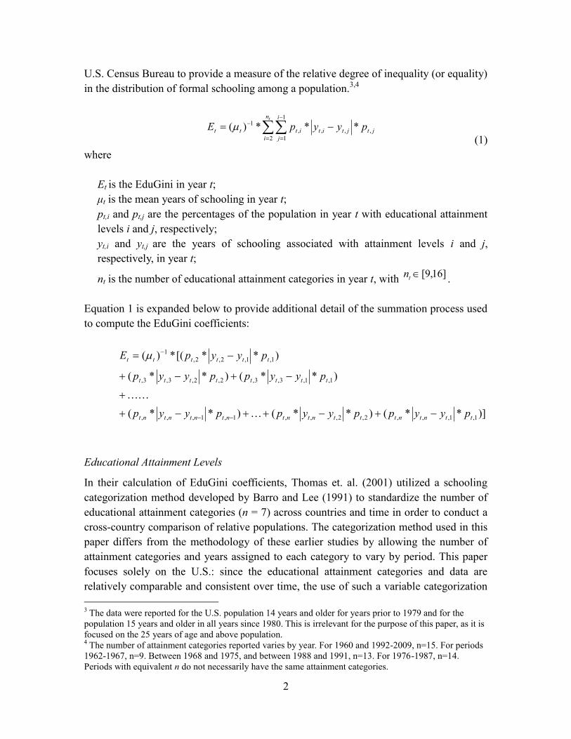
U.S. Census Bureau to provide a measure of the relative degree of inequality (or equality) in the distribution of formal schooling among a population.3,4

jt

n

i

i

jjtitittt pyypE

t

,2

1

1,,,

1 ***)(

(1) where

Et is the EduGini in year t; μt is the mean years of schooling in year t; pt,i and pt,j are the percentages of the population in year t with educational attainment levels i and j, respectively; yt,i and yt,j are the years of schooling associated with attainment levels i and j, respectively, in year t;

nt is the number of educational attainment categories in year t, with ]16,9[tn . Equation 1 is expanded below to provide additional detail of the summation process used to compute the EduGini coefficients:

)]**()**()**(

)**()**(

)**[(*)(

1,1,,,2,2,,,1,1,,,

1,1,3,3,2,2,3,3,

1,1,2,2,1

ttntntttntntntntntnt

tttttttt

tttttt

pyyppyyppyyp

pyyppyyp

pyypE

Educational Attainment Levels

In their calculation of EduGini coefficients, Thomas et. al. (2001) utilized a schooling categorization method developed by Barro and Lee (1991) to standardize the number of educational attainment categories (n = 7) across countries and time in order to conduct a cross-country comparison of relative populations. The categorization method used in this paper differs from the methodology of these earlier studies by allowing the number of attainment categories and years assigned to each category to vary by period. This paper focuses solely on the U.S.: since the educational attainment categories and data are relatively comparable and consistent over time, the use of such a variable categorization 3 The data were reported for the U.S. population 14 years and older for years prior to 1979 and for the population 15 years and older in all years since 1980. This is irrelevant for the purpose of this paper, as it is focused on the 25 years of age and above population. 4 The number of attainment categories reported varies by year. For 1960 and 1992-2009, n=15. For periods 1962-1967, n=9. Between 1968 and 1975, and between 1988 and 1991, n=13. For 1976-1987, n=14. Periods with equivalent n do not necessarily have the same attainment categories.

3

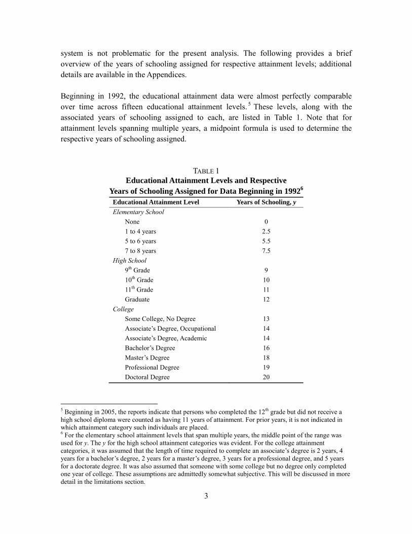
system is not problematic for the present analysis. The following provides a brief overview of the years of schooling assigned for respective attainment levels; additional details are available in the Appendices. Beginning in 1992, the educational attainment data were almost perfectly comparable over time across fifteen educational attainment levels. 5 These levels, along with the associated years of schooling assigned to each, are listed in Table 1. Note that for attainment levels spanning multiple years, a midpoint formula is used to determine the respective years of schooling assigned.

TABLE 1 Educational Attainment Levels and Respective

Years of Schooling Assigned for Data Beginning in 19926

Educational Attainment Level Years of Schooling, y Elementary School

None 0 1 to 4 years 2.5 5 to 6 years 5.5 7 to 8 years 7.5

High School 9th Grade 9 10th Grade 10 11th Grade 11 Graduate 12

College Some College, No Degree 13 Associate’s Degree, Occupational 14 Associate’s Degree, Academic 14 Bachelor’s Degree 16 Master’s Degree 18 Professional Degree 19 Doctoral Degree 20

5 Beginning in 2005, the reports indicate that persons who completed the 12th grade but did not receive a high school diploma were counted as having 11 years of attainment. For prior years, it is not indicated in which attainment category such individuals are placed. 6 For the elementary school attainment levels that span multiple years, the middle point of the range was used for y. The y for the high school attainment categories was evident. For the college attainment categories, it was assumed that the length of time required to complete an associate’s degree is 2 years, 4 years for a bachelor’s degree, 2 years for a master’s degree, 3 years for a professional degree, and 5 years for a doctorate degree. It was also assumed that someone with some college but no degree only completed one year of college. These assumptions are admittedly somewhat subjective. This will be discussed in more detail in the limitations section.

4

Prior to 1992, there were some differences in the number and reporting of attainment categories over time. Generally speaking, the same methods as described above (particularly the midpoint formula for attainment categories spanning several school levels) were used to derive the years of schooling associated with each category. The first difference in the data is that the number of different attainment categories was not consistent prior to 1992 due to changes in reporting by the Census Bureau. As noted above, the number of attainment categories ranged from nine to sixteen This was a relatively minor issue that was dealt with by allowing the number of attainment categories to vary by year and assigning the appropriate years of schooling to each category for every year, as indicated in Equation 1 above. The more difficult issue was that several of the attainment categories differed significantly over the period of study. This merited the implementation of interpolation techniques intended to increase the accuracy of the estimates for mean years of schooling (MYS) over particular periods of time, thereby increasing the accuracy of the EduGini. These methodological techniques are described in the Appendix A.

III. Understanding the EduGini

The EduGini measures the relative distribution of education among a population, and it provides additional information beyond that of traditional macro-level measures of education such as graduation rates or average years of educational attainment. As previously indicated (see Equation 1), the EduGini measure is a function of the years of schooling associated with the various levels of schooling, the percentage of the population with each level of educational attainment, and the average educational attainment of the population. Prior to discussing the actual results, some hypothetical EduGini measures are described to help the reader better conceptualize what information the EduGini conveys. The EduGini ranges from zero to one, with a value of zero indicating that all persons among a population have attained an equal amount of schooling, implying ―perfect equality‖ in the distribution of education, and a value of one resulting from one person having attained all of the aggregate education, with everyone else attaining none, signifying ―perfect inequality.‖ Zero and one are the two extreme values and are mostly theoretical, as neither extreme is likely to occur, nor should either necessarily be a desirable goal. An example of ―perfect inequality‖ with an EduGini value of 1 may be illustrated as the result of a repressive island economy in which the tyrannical dictator ventures mainland to attain a Ph.D. in Medieval Monarchy and Serfdom while the remainder of the population, the dictator’s serfs, have no opportunity to attend school and are unable to escape the island. This is quite obviously an undesirable outcome. The less

5

obvious reason why the opposite outcome of ―perfect equality‖ may be similarly undesirable is not nearly as obvious and requires more explanation. The ―perfect equality‖ indicated by an EduGini value of zero implies that everyone has exactly the same number of years of schooling. While this may sound ideal, it is important to keep in mind that any population consists of a diverse set of individuals who differ in their ability to learn and to access educational opportunities. These individuals also hold different attitudes towards risk and expect different returns from their investment in education.7 They may also differ in their preferences for education relative to alternative allocations of time (Becker and Chiswick, 1966). Since the demand for various levels of education is not inherently homogenous, perfect equality in the distribution of educational attainment is neither desirable nor practical. The real world consists of various economic agents which have competing interests for the use of scarce resources and limited time.

Next, consider other , slightly more plausible example:. Hypothesize a case in which half of the adult population has zero formal education and the other half has a high school diploma. Using the methodology employed in this paper, the average educational attainment of the population would be 6 years of schooling, and the resulting EduGini measure would be 0.5.8 If instead of a high school diploma, half of the population had a bachelor’s degree (BA) while the other half still had no education, then the average attainment level would increase to 8 years of schooling, but the EduGini measure would remain 0.5 since educational inequality was unchanged. Table 2 provides the percent of the population with the respective attainment levels, mean years of schooling, and EduGini value for the previously described hypothetical distributions, as well as a few slightly more complicated hypothetical distributions. Now, if instead of no education, half of the population completed the 8th grade and the other half had a high school diploma, then the average attainment level would increase to 10 years of schooling and the EduGini would decrease significantly to 0.1, signifying a reduction in educational inequality of 80 percent from the previous example. Now assume that half of the population still has an 8th grade education, but the other half now possesses a bachelor’s degree instead of only a high school diploma. The average attainment level would increase to 12 years of schooling, but the EduGini would rise to 0.167 in this case. If the half of the population with only an 8th grade education completed high school, then the average attainment level would increase to 14 years of

7 This is true to the extent that formal education is considered an investment in human capital formulation rather than a consumption good or service 8 Note that had we replaced ―high school diploma‖ with any other attainment level greater than zero, it would have resulted in a value of 0.5 as well

6

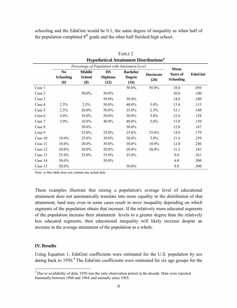
schooling and the EduGini would be 0.1, the same degree of inequality as when half of the population completed 8th grade and the other half finished high school.

TABLE 2 Hypothetical Attainment Distributions

a

Percentage of Population with Attainment Level Mean

Years of

Schooling

EduGini

No

Schooling

(0)

Middle

School

(8)

HS

Diploma

(12)

Bachelor

Degree

(16)

Doctorate

(20)

Case 1 50.0% 50.0% 18.0 .056 Case 2 50.0% 50.0% 10.0 .100 Case 3 50.0% 50.0% 14.0 .100 Case 4 2.5% 2.5% 50.0% 40.0% 5.0% 13.6 .115 Case 5 2.5% 20.0% 50.0% 25.0% 2.5% 12.1 .148 Case 6 5.0% 10.0% 50.0% 30.0% 5.0% 12.6 .158 Case 7 5.0% 10.0% 40.0% 40.0% 5.0% 13.0 .159 Case 8 50.0% 50.0% 12.0 .167 Case 9 25.0% 25.0% 25.0% 25.0% 14.0 .179 Case 10 10.0% 25.0% 30.0% 30.0% 5.0% 11.4 .239 Case 11 10.0% 20.0% 30.0% 30.0% 10.0% 12.0 .240 Case 12 20.0% 20.0% 20.0% 20.0% 20.0% 11.2 .343 Case 13 25.0% 25.0% 25.0% 25.0% 9.0 .361 Case 14 50.0% 50.0% 6.0 .500 Case 15 50.0% 50.0% 8.0 .500 Note: a=this table does not contain any actual data These examples illustrate that raising a population's average level of educational attainment does not automatically translate into more equality in the distribution of that attainment, Iand may even in some cases result in more inequality depending on which segments of the population obtain that increase. If the relatively more educated segments of the population increase their attainment levels to a greater degree than the relatively less educated segments, then educational inequality will likely increase despite an increase in the average attainment of the population as a whole.

IV. Results

Using Equation 1, EduGini coefficients were estimated for the U.S. population by sex dating back to 1950.9 The EduGini coefficients were estimated for six age groups for the

9 Due to availability of data, 1950 was the only observation period in the decade. Data were reported biannually between 1960 and 1964, and annually since 1965.

7

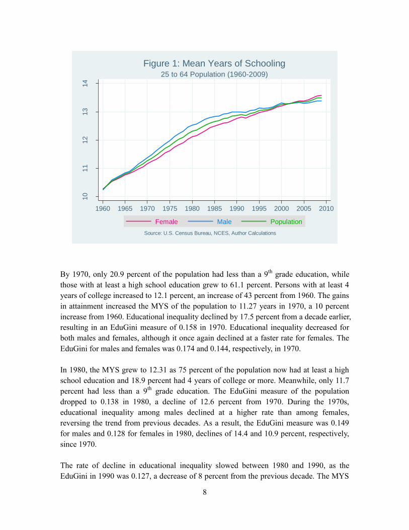
time periods indicated, as well as for the entire adult population aged 25 to 64.10 The estimates generally indicate a greater degree of educational inequality among older subpopulations (relative to younger age groups), with the difference in EduGini coefficient between relatively older and younger subpopulations declining over time. The results discussed in this section will focus on the 25-64 population, including separate EduGini estimates for the male and female subpopulations, since this age span is a good measure of the post-schooling, working-age adult population. Appendices 2A-2C contains tables that report the EduGini coefficients by age group and sex. From this point forward, discussion will refer exclusively to the 25-64 population unless otherwise noted. In 1950, the MYS was 9.46 years, as 44.4 percent of the population had less than a 9th grade education, 37 percent had at least a high school education, and only 6.6 percent had attained 4 years of college or more. Using the complete attainment data, the EduGini was 0.213 for the U.S. in 1950.11 The MYS was higher for females (9.56) than males (9.35) in 1950, with educational inequality greater among males than females, as the EduGini measures were 0.224 and 0.205, respectively. Figure 1 shows the change in MYS of the population by sex over time. By 1960, the MYS of the population grew to 10.25 years, an increase of 8.3 percent from 1950. Persons with less than a 9th grade education in 1960 declined to 34 percent, a 23.4 percent decrease since 1950. The percent with a high school education or more increased to 45.3, an increase of 22.5 percent over the decade. Meanwhile, the percent with at least 4 years of college grew to 8.4, an increase of 27.2 percent from 1950. The EduGini declined to 0.192 in 1960, a decrease of 9.8 percent from 1950. Educational inequality declined at a faster rate for females than males over the decade, further widening the gap between the sexes. The EduGini measure in 1960 was 0.208 for males and 0.178 for females, decreases of 7.4 and 13.3 percent from 1950, respectively.

10 The subpopulations include the 18-24, 25-34, 35-44, 45-54, 55-64, and 65+ age groups. 11 Less than 9 years refers to 8 years or less. At least high school education refers to 12 years of attainment or more. There were a total of 14 attainment categories in 1950. The figures cited do not correspond to the categories but are intended to give the reader a reference of how certain attainment benchmarks have changed over time.

8

By 1970, only 20.9 percent of the population had less than a 9th grade education, while those with at least a high school education grew to 61.1 percent. Persons with at least 4 years of college increased to 12.1 percent, an increase of 43 percent from 1960. The gains in attainment increased the MYS of the population to 11.27 years in 1970, a 10 percent increase from 1960. Educational inequality declined by 17.5 percent from a decade earlier, resulting in an EduGini measure of 0.158 in 1970. Educational inequality decreased for both males and females, although it once again declined at a faster rate for females. The EduGini for males and females was 0.174 and 0.144, respectively, in 1970. In 1980, the MYS grew to 12.31 as 75 percent of the population now had at least a high school education and 18.9 percent had 4 years of college or more. Meanwhile, only 11.7 percent had less than a 9th grade education. The EduGini measure of the population dropped to 0.138 in 1980, a decline of 12.6 percent from 1970. During the 1970s, educational inequality among males declined at a higher rate than among females, reversing the trend from previous decades. As a result, the EduGini measure was 0.149 for males and 0.128 for females in 1980, declines of 14.4 and 10.9 percent, respectively, since 1970. The rate of decline in educational inequality slowed between 1980 and 1990, as the EduGini in 1990 was 0.127, a decrease of 8 percent from the previous decade. The MYS

10

11

12

13

14

Mean Y

ears

of

Schoolin

g

1960 1965 1970 1975 1980 1985 1990 1995 2000 2005 2010

Female Male Population

Source: U.S. Census Bureau, NCES, Author Calculations

25 to 64 Population (1960-2009)

Figure 1: Mean Years of Schooling

9

also grew at a slower pace than previous decades, increasing by 4.6 percent from 1980 to 12.88 years. In 1990, 7.2 percent of the populace remained with less than a 9th grade education, while the percent with at least a high school education grew to 82.8 percent. Persons with 4 years of college or more increased to 23.5 percent. The EduGini once again declined at a faster rate for males than females between 1980 and 1990, as the measures declined to 0.134 for males and 0.12 for females in 1990. As described in Section II above, there was a change in the educational attainment categories reported by the Census Bureau in 1992. As indicated in Figure 2, which shows the trend in U.S. EduGini coefficients between 1960 and 2009, this categorical change is likely the reason for the level shift of the EduGini measure between 1991 and 1992. As such, comparing the attainment data and resulting statistics prior to 1992 with post-1992 data should be done with this categorical difference in mind.

The segment of the population with less than a 9th grade education declined to 4.7 percent by 2000. Meanwhile the share with at least a high school education increased to 87.5 percent, with 28 percent having attained a bachelor’s degree or higher, increases of 4 and

1992 Attainment Category Change

0.1

00.1

20.1

40.1

60.1

80.2

0

EduG

ini

1960 1965 1970 1975 1980 1985 1990 1995 2000 2005 2010

Female Male Population

Source: U.S. Census Bureau, NCES, Author Calculations

25 to 64 Population (1960-2009)

Figure 2: Education Gini

10

18.7 percent, respectively, since 1992.12 The MYS was 13.26 years in 2000, an increase of 3 percent from 1992. Educational inequality decreased by 2.3 percent between 1992 and 2000, as the EduGini measure for the population fell to 0.115 in 2000. The gender gap in educational inequality continued to decline during the 1990s, as the EduGini for males was 0.118 in 2000, and 0.11 for females. The EduGini measure declined slightly between 2000 and 2009 to 0.112, as the MYS increased modestly to 13.48 years. Only 4.2 percent of the population remained with less than a 9th grade education, while the percent with at least a high school education increased slightly to 88.6 in 2009. Although the percentage of college graduates increased to 31.4 in 2009, the rate of growth slowed from that experienced in previous periods. Educational inequality between males and females neared parity in 2009, as the EduGini measures were 0.116 and 0.111, respectively.

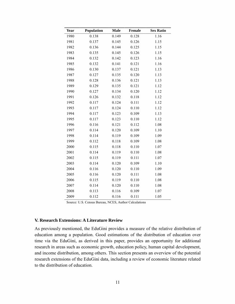
Table 3 summarizes the EduGini coefficients for the 25-64 population over the period of study, including the male to female EduGini ratio.

TABLE 3 EduGini by Year, Sex for 25-64 Population

Year Population Male Female Sex Ratio

1950 0.213 0.224 0.205 1.10 1960 0.192 0.208 0.178 1.17 1962 0.184 0.200 0.167 1.19 1964 0.175 0.192 0.158 1.21 1965 0.173 0.190 0.156 1.22 1966 0.171 0.188 0.154 1.22 1967 0.168 0.184 0.153 1.20 1968 0.166 0.182 0.151 1.20 1969 0.163 0.178 0.149 1.20 1970 0.158 0.174 0.144 1.21 1971 0.157 0.171 0.141 1.21 1972 0.154 0.167 0.140 1.19 1973 0.152 0.164 0.138 1.19 1974 0.150 0.164 0.135 1.21 1975 0.148 0.161 0.134 1.20 1976 0.147 0.158 0.132 1.20 1977 0.146 0.157 0.132 1.20 1978 0.143 0.155 0.131 1.18 1979 0.140 0.151 0.129 1.17

12 In 1992, the data began reporting persons with a bachelor’s degree rather than number of years of college. In 2005, persons with 12 years of schooling but no high school diploma began being reported as having 11 years of schooling. For these reasons, 1992 is used as a benchmark here rather than 1990.

11

Year Population Male Female Sex Ratio

1980 0.138 0.149 0.128 1.16 1981 0.137 0.145 0.126 1.15 1982 0.136 0.144 0.125 1.15 1983 0.135 0.145 0.126 1.15 1984 0.132 0.142 0.123 1.16 1985 0.132 0.141 0.121 1.16 1986 0.130 0.137 0.121 1.13 1987 0.127 0.135 0.120 1.13 1988 0.128 0.136 0.121 1.13 1989 0.129 0.135 0.121 1.12 1990 0.127 0.134 0.120 1.12 1991 0.126 0.132 0.118 1.12 1992 0.117 0.124 0.111 1.12 1993 0.117 0.124 0.110 1.12 1994 0.117 0.123 0.109 1.13 1995 0.117 0.123 0.110 1.12 1996 0.116 0.121 0.112 1.08 1997 0.114 0.120 0.109 1.10 1998 0.114 0.119 0.109 1.09 1999 0.112 0.118 0.109 1.08 2000 0.115 0.118 0.110 1.07 2001 0.114 0.119 0.110 1.08 2002 0.115 0.119 0.111 1.07 2003 0.114 0.120 0.109 1.10 2004 0.116 0.120 0.110 1.09 2005 0.116 0.120 0.111 1.08 2006 0.115 0.119 0.110 1.08 2007 0.114 0.120 0.110 1.08 2008 0.113 0.116 0.109 1.07 2009 0.112 0.116 0.111 1.05 Source: U.S. Census Bureau, NCES, Author Calculations

V. Research Extensions: A Literature Review

As previously mentioned, the EduGini provides a measure of the relative distribution of education among a population. Good estimations of the distribution of education over time via the EduGini, as derived in this paper, provides an opportunity for additional research in areas such as economic growth, education policy, human capital development, and income distribution, among others. This section presents an overview of the potential research extensions of the EduGini data, including a review of economic literature related to the distribution of education.

12

Evaluating Education Policy

In terms of shaping and evaluating educational policy, the EduGini is a particularly valuable measure because politicians on both sides of the aisle have generally supported allocating billions of dollars for the express purpose of increasing educational opportunities. A measure of the relative distribution of educational attainment makes it possible to evaluate the effectiveness and equitableness of education policies intended to encourage and increase educational opportunities. One cross-country study found that the level of educational expenditures is not significantly related to the ―degree of equality of educational opportunity achieved (Schuetz, Ursprung, Woessman, 2005).‖ Human Capital Development and Economic Growth

To the extent that formal education develops human capital, EduGini may provide a useful measure of the distribution of the latter. This distribution may be an important factor for economic growth, as human capital is a key endogenous variable in much of the growth literature (e.g., Lucas (1988); Romer (1990)). 13 As Hanushek and Wößmann (2010) noted:

First, education can increase the human capital inherent in the labor force, which increases labor productivity and thus transitional growth towards a higher equilibrium level of output. Second, education can increase the innovative capacity of the economy, and the new knowledge on new technologies, products and processes promotes growth, Third, education can facilitate the diffusion and transmission of knowledge needed to understand and process new information and to implement successfully new technologies devised by others, which again promotes economic growth.

Thomas, Wang and Fan (2001) described the importance of the dispersion of human capital in production, suggesting that:

The distributional dimension of education is extremely important for both welfare consideration and for production. If an asset, say physical capital, is freely traded across firms in a competitive environment, its marginal product will be equalized through free-market mechanism. As a result, its contribution to output will not be

13 Preliminary work by CCAP suggests that a significant portion of human capital development, as measured by lifetime earning power, is attributable to informal learning-by-doing, or on-the-job training, suggesting that the effect of formal education on human capital formulation may be less than many believe. In addition, Hanushek and Wößmann (2010) note that ―using years of schooling implicitly assumes that all skills and human capital come from formal schooling. Yet extensive evidence on knowledge development and cognitive skills indicates that a variety of factors outside of school—family, peers, and others— have a direct and powerful influence.‖

13

affected by its distribution across firms or individuals. If an asset is not completely tradable, however, then the marginal product of the asset across individuals is not equalized, and there is an aggregation problem. In this case, aggregate production function depends not only on the average level of the asset but also on its distribution. Because education/skill is only partially tradable, the average level of educational attainment alone is not sufficient to reflect the characteristics of a country's human capital. We need to look beyond averages and investigate… [the] dispersion of human capital.

However, in a cross-country analysis, Schuetz, Ursprung, Woessman (2005) found that the degree of equality of educational opportunity achieved exhibited an insignificant affect on economic growth. Work by Hanushek and Wößmann (2010) provides a plausible explanation as they suggest that not all education is equal in terms of inducing positive economic outcomes, warning that ―ignoring differences in the quality of education significantly distorts the picture of how educational and economic outcomes are related.‖ The Relationship between the Distribution of Education and Income

Of particular interest in the literature has been the effect of educational inequality on the distribution of income, but the direction and magnitude of the effect, as well as the direction of causality, remain ambiguous. Some researchers have theorized and found empirical evidence that reductions in educational inequality have an equalizing effect on the distribution of income. While there is no consensus on the role that the distribution of education plays in determining the distribution of income, data for the U.S. since 1960 show a clear divergence between the two measures. Over the past 50 years, educational inequality has decreased significantly while income inequality has increased as indicated in Figure 3.14 A review of the literature related to the relationship between the distribution of education and income is discussed next.

14 Note that there are two income inequality measures charted: income inequality among families and among households.

14

In a cross-country panel data analysis, De Gregorio and Lee (2002) found some evidence that higher levels of educational attainment and more equal distribution of education have an effect on changing the level of income distribution, with higher levels of attainment being negatively correlated, and more equal distribution of education positively correlated with income inequality. Their results were limited by the fact that regional factors and social expenditures were found to be significant in reducing income inequality and that a ―significant proportion of the variation in income inequality across countries and over time remains unexplained.‖ Work by Becker and Chiswick (1966) theorizes that greater rates of return from human capital investments and inequality in the distribution of schooling have a positive effect on earnings inequality and find evidence that schooling ―explains a not negligible part of the inequality in earnings within a geographical area and a much larger part of differences in inequality between areas.‖ Knight and Sabot (1983) suggested that changes in the educational composition of the labor force have an ambiguous effect on the dispersion of earnings, inducing a Kuznets effect in which initially, the ―compositional‖ effect increases the average educational level of a population that benefits only a small portion of the population, increasing their earnings potential relative to the rest of the population, thereby increasing income

.1.1

5.2

.25

.3.3

5.4

.45

.5

Gin

i C

oe

ffic

ien

t

1960 1965 1970 1975 1980 1985 1990 1995 2000 2005 2010

Education Family Income Household Income

Source: U.S. Census Bureau, NCES, Author Calculations (EduGini)

(1960 - 2009)

Figure 3: Education vs. Income Inequality

15

inequality. However, the premium or return from education is expected to fall as the distribution of education widens and hence, the supply of educated workers increases relative to the labor market demand, leading to a wage compression effect that reduces inequality. Other research has found that there is ―no adverse effect of educational inequality on income distribution,‖ (Ram, 1984) with empirical evidence from developing countries indicating that ―despite fairly substantial educational expansion…there is hardly any sign of an improvement in income distribution‖ (Ram, 1990). Some research, exploiting Spence’s education as a signaling device hypothesis, has suggested that public policy intended to make education (particularly of the postsecondary variety) more accessible and affordable can make the distribution of education more equal; but, in doing so, leads to greater income inequality as the average ability of workers in the low education pool declines, driving down their wages while simultaneously raising the wage premium for the highly skilled (Hendel, Shapiro and Willen, 2005). Another paper reached a similar conclusion, remarking that in a human capital screening environment, ―Anything that encourages good workers to get educated can set in motion a cumulative process of growing inequality (Krugman, 2000).‖

VI. Conclusions

The EduGini measures reported in this paper indicate that educational inequality has declined over time in the United States, although the rate of decline has slowed significantly during the last two decades. In fact, the EduGini measure declined from 0.213 to 0.126 between 1950 and 1991, the last year before the new educational attainment classification system was in place. Of this decline, 24 percent occurred by 1960 and 45.6 percent by 1965, the year in which the two major federal education programs were initially enacted.15 By 1975, 74.2 percent of the decline had occurred, with another 11.5 percent occurring by 1980. Only 14.3 percent of the decline occurred between 1980 and 1991. Since 1992, the EduGini has been relatively constant, declining from 0.117 to 0.112 in 2009, a 4.3 percent decline. Educational inequality has historically been greater among the male than the female population. The gap between the sexes widened between 1950 and the early 1970s, remaining relatively high throughout most of the 1970s before beginning to fall. Since then, the rate of decline in EduGini has been faster for the male population than the female, resulting in a closing of the gap. Today, the EduGini measures for males and

15 The Higher Education Act and Elementary and Secondary Education Act were both legislated in 1965

16

females are near parity, suggesting that educational inequality is about the same for both sexes, although females have recently achieved a higher average attainment. The EduGini measures were developed using large sample government attainment data and as such, are assumed to be fairly accurate estimates of the actual attainment levels and hence, inequality in the distribution of education of the U.S. population. While the EduGini measures provide good indicators of the quantity of education received in the U.S. and the distribution of it, they do not account for potential differences in the quality (e.g., cognitive skill development) of education received, or the distribution of educational quality among the population. Measures of education quality are actually rather opaque and therefore beyond the scope of this paper. As such, the attainment levels and corresponding EduGini coefficients reported here are not sufficient measures of the quality of education among the U.S. population, and should not be treated as such. Future CCAP research will explore the economic implications of the distribution of education and the EduGini measures, including how changes in the demographic, economic, and socio-political environments have affected the distribution of education in the United States.

17

Appendix A: Full Methodology

The EduGini for the United States is calculated by year, age group, and sex, adopting a formula developed by Thomas, Wang, and Fan (2001). They modified the Gini coefficient formula that is often used to calculate income inequality by utilizing educational attainment data of a country’s population to calculate an education Gini index to measure the relative inequality (or equality) in the distribution of education among a population. This formula, although modified slightly since this paper is focused solely on the U.S. population, is given in Equation (1) above.

Educational attainment data from the U.S. Census Bureau were the primary data used to compute education Gini coefficients for the U.S. population by age group and sex for the periods indicated. National Center for Education Statistics (NCES) data on degrees awarded, as discussed below, augmented the attainment data. Due to limitations in the availability of attainment data, there are no observations between 1950 and 1960. Data was reported on a biannual basis between 1960 and 1964, and annually beginning in 1965. The data were reported for the U.S. population 14 years and older for years prior to 1979, and for the 15 years and above population in all years since 1980. This is irrelevant for the purpose of this paper, as it is focused on the 18 years of age and above population.

The attainment data were grouped into seven age categories that were consistently reported over time and are discussed below. This age differentiation approach differs from that used by Thomas, et.al. (2001), who estimated mean years of schooling and education Gini for the entire 15+ years of age population and allows for more meaningful measures to be developed and used for analytical purposes. Age Groups

Since most Americans under the age of 18 have not completed their formal education, and most remain in the education system, the analysis in this paper ignores this age group.16 Instead, it focuses on the population above 18 years of age, with a particular emphasis on the population 25 to 64 years of age since this is an age by which most persons have traditionally completed their formal education and entered the working stage of their life. The data were divided into seven age groups that were used to develop EduGini coefficients for each time period for the respective populations and by sex. Doing so

16 According to data reported by the U.S. Department of Education (NCES), more than 90 percent of 14-to-17 year olds have been enrolled in school since around 1960, with the percentage reaching nearly 97 percent in 2008. For the 7-to-13 year old population, more than 95 percent have been enrolled in school since 1950, with the figure reaching nearly 99 percent in 2008.

18

provides us with useful metrics to determine how the distribution of educational attainment varies by age and sex over time. The educational attainment data were grouped into the following seven age categories for which data were consistently available across time periods: 25 to 64 years of age (25-64) 18 to 24 years of age (18-24) 25 to 34 years of age (25-34) 35 to 44 years of age (35-44) 45 to 54 years of age (45-54) 55 to 64 years of age (55-64) 65 years of age and above (65+) Attainment Levels

As discussed in section III, the number of attainment categories and years of schooling assigned to each were allowed to vary over time, although the data is nearly perfectly compatible across years beginning in 1992. Due to some limitations in the data, several interpolation techniques were employed in an effort to increase the accuracy of the MYS and EduGini estimates for different periods of study. These techniques were briefly mentioned above, but a complete description of each technique follows. Interpolation Technique 1: Pre-1992 Advanced College Data

The most significant difference between the pre- and post-1992 data was in the reporting of advanced college degree attainment. Beginning in 1992, advanced college attainment data are reported by degree level (i.e., master’s, professional, and doctorate), which makes the task of assigning the years of schooling associated with each degree level a relatively straightforward exercise. Prior to 1992, however, there was only a single advanced college attainment category (5+ years), making it very difficult to assign an appropriate value to the years of schooling for the category. In order to more accurately estimate the years of schooling associated with the 5+ years of college attainment category, and consequently the MYS and EduGini coefficients, for each year prior to 1992, historical NCES data on the number of degrees awarded by degree level and decade were used to develop weighted mean years of attainment associated with the advanced college attainment (5+ years) category by year and for the various age categories, utilizing simple averages from recent decennial periods

19

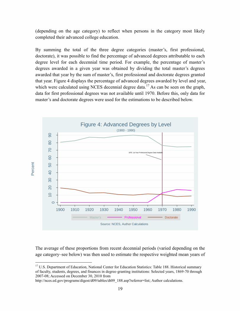
(depending on the age category) to reflect when persons in the category most likely completed their advanced college education. By summing the total of the three degree categories (master’s, first professional, doctorate), it was possible to find the percentage of advanced degrees attributable to each degree level for each decennial time period. For example, the percentage of master’s degrees awarded in a given year was obtained by dividing the total master’s degrees awarded that year by the sum of master’s, first professional and doctorate degrees granted that year. Figure 4 displays the percentage of advanced degrees awarded by level and year, which were calculated using NCES decennial degree data.17 As can be seen on the graph, data for first professional degrees was not available until 1970. Before this, only data for master’s and doctorate degrees were used for the estimations to be described below.

The average of these proportions from recent decennial periods (varied depending on the age category–see below) was then used to estimate the respective weighted mean years of 17 U.S. Department of Education, National Center for Education Statistics: Table 188. Historical summary of faculty, students, degrees, and finances in degree-granting institutions: Selected years, 1869-70 through 2007-08; Accessed on December 30, 2010 from http://nces.ed.gov/programs/digest/d09/tables/dt09_188.asp?referrer=list; Author calculations.

1970: 1st Year Profesional Degree Data Available

010

20

30

40

50

60

70

80

90

Perc

ent

1900 1910 1920 1930 1940 1950 1960 1970 1980 1990

Master's Professional Doctorate

Source: NCES, Author Calculations

(1900 - 1990)

Figure 4: Advanced Degrees by Level

20

schooling associated with the 5+ years of college attainment category for each year and age category using Equation (2),

n

ypn

j kkjk

ht

1

3

1*

(2)

where ht is the mean years of advanced college education (the 5+ years category) for age

group h in year t, jkp is the percentage of advanced degrees awarded at level k18 in

decennial period j, ky is the years of schooling associated with degree level k, and n is the

number of decennial periods used to calculate the mean years of schooling, ht , for age group h in year t.

18 k={k1, k2, k3} ={master’s, first professional, doctorate}

21

Because EduGini coefficients are estimated over time for six different age categories,

estimates of the mean years of advanced college education, ht for each h are necessary.19 Given that the age of persons in each h varies and as such, they likely completed their schooling at different periods of time, the number of decennial periods, n, used to

estimate each age groups’ average years of advanced college education, ht , varies to reflect the time when persons likely completed their advanced college education. Using this methodology provides a more accurate estimate of the MYS for persons with 5+ years of college education, and hence, a more accurate EduGini estimate. For the 18-24 population, the proportion of advanced college degrees awarded at level k, pk, from the most recent decennial period was used, as these persons would have been enrolled in school very recently. For years whose last digit was between 19x0 and 19x7, the preceding decade’s degree data were used; whereas for years whose last digit was 19x8 or 19x9, the forthcoming decade’s degree data were used. For example, to estimate for the 18-24 population in 1977, pk from 1970 was used, whereas for 1978, pk from 1980 was used. This same methodology is used for the remaining age categories with respect to the most recent decennial period in order to provide a more accurate estimate of . For the 25-64 population, the simple average of the pk from the preceding five decennial periods was used to estimate , as persons in this age category, depending on their age, likely completed their formal college education spanning the previous five decades (the closest decennial period used according to the last digit of year, as discussed above). For the 25-34 population, a simple average of the pk from the preceding two decennial periods was used to estimate , as persons in this age category likely completed their college education during one of the two periods. For the 35-44 population, a simple average of the pk from the three most recent decennial periods was used to estimate , as persons in this age range may have attended school during any of the three. For the 45-54 population, a simple average of the pk from the preceding four decennial periods, minus the most recent one, was used to estimate , as persons in this age category likely completed their college education in the preceding forty years, but unlikely completed it very recently. For both the 55-64 and 65+ populations, a simple average of the pk from the preceding five decennial periods, minus the two most recent ones, was used to estimate , as persons in these two age categories likely did not attend college very recently, but likely did so sometime in the preceding fifty years.

19 hl = {25-64, 18-24, 25-34, 35-44, 45-54, 55-64}

22

Interpolation Technique 2: 1968 to 1975 Elementary Schooling Data

Differences in the data also required an interpolation technique to estimate the years of schooling for the 0 to 4 years of educational attainment category for the years between 1968 and 1975. This was deemed significant since all other years included a single category for persons with zero years of schooling, and a separate category for persons with between one and four years of schooling.

The weighted average years of schooling, wh , for persons in age group h with 0 and 1-4 years of schooling were found for both the immediately prior period (1967) and the immediately following period (1976) using Equation (3):

I

iih

I

iihih

hp

pyw

1

1

(3)

Where pih is the number of persons in age group h with i years of schooling and yih is the years of schooling associated with attainment category i for age group h. Next, the simple average of wh from 1967 and 1976 was taken to estimate the average years of schooling associated with the ―0-4‖ attainment category for the 1968 to 1975 periods.

Using the middle point of the range formula as previously described would have resulted in nontrivial overestimation of the years of schooling for persons in the 0-4 category between 1968 and 1975, as it would have assigned a y of 2.5. The interpolation technique just described produced a y that varied by age group, hl, ranging from 1.32 for the 18-24 group to 1.97 for both the 45-54 and 55-64 age groups.

Interpolation Techniques 3/4: 1962 to 1967 High School and College Data

For the periods between 1962 and 1967, the data for both high school and undergraduate college education included only two categories, 1-3 and 4 years of schooling, whereas all other years listed single years of high school and college attained. 20 A similar interpolation technique as the one previously described was used to estimate the years of schooling yih associated with each of these two categories, with the only differences being

that the weighted averages, hw ,were calculated for persons with one, two and three years of high school (or college) in both 1960 and 1968, and the simple average of the two years was taken to derive the average years of schooling associated with the high school (or college) 1-3 years of attainment category for the 1962 to 1967 periods. The resulting 20 The exception being the post-1992 college attainment data, as discussed above.

23

years of schooling for the high school and college 1-3 categories ranged from 9.8 for the 65+ group to 10.2 for the 18-24 group, while it ranged from 13.74 for the 18-24 group to 13.83 for the 65+ group, respectively. The midpoint of the range formula would have resulting in assigning values of 10 and 14 for the two attainment categories, respectively, for all age groups.

Mean Years of Schooling

Mean years of schooling, ht , were computed for each age group, h, and year, t, according to Equation (4):

K

khtkhtkht yp

1*

(4)

where htkp is the percentage of the population of age group h in year t with educational attainment level k, and yhtk is the years of schooling associated with attainment level k for age group h in year t. As stated above, grouping the data by age category is useful for analytical purposes, because the equation for computing EduGini coefficients relies on mean years of school, and there is an inverse relationship between age group and average educational attainment. In other words, younger age groups have higher mean years of schooling. This is not surprising since the average educational attainment has generally increased in the U.S. with each successive generation. Figure 5 displays the computed mean years of schooling for each of the age groups by year between 1960 and 2009.

24

78

910

11

12

13

14

MY

S

1960 1965 1970 1975 1980 1985 1990 1995 2000 2005 2010

18-24 25-34

35-44 45-54

55-64 65+

Source: U.S. Census Bureau, NCES, Author Calculations

by Age Group (1960 - 2009)

Figure 5: Mean Years of Schooling

25

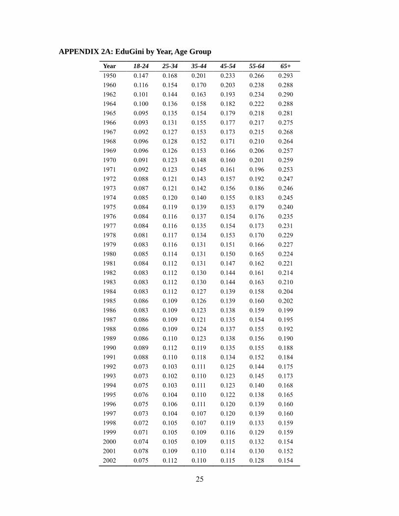
APPENDIX 2A: EduGini by Year, Age Group

Year 18-24 25-34 35-44 45-54 55-64 65+

1950 0.147 0.168 0.201 0.233 0.266 0.293 1960 0.116 0.154 0.170 0.203 0.238 0.288 1962 0.101 0.144 0.163 0.193 0.234 0.290 1964 0.100 0.136 0.158 0.182 0.222 0.288 1965 0.095 0.135 0.154 0.179 0.218 0.281 1966 0.093 0.131 0.155 0.177 0.217 0.275 1967 0.092 0.127 0.153 0.173 0.215 0.268 1968 0.096 0.128 0.152 0.171 0.210 0.264 1969 0.096 0.126 0.153 0.166 0.206 0.257 1970 0.091 0.123 0.148 0.160 0.201 0.259 1971 0.092 0.123 0.145 0.161 0.196 0.253 1972 0.088 0.121 0.143 0.157 0.192 0.247 1973 0.087 0.121 0.142 0.156 0.186 0.246 1974 0.085 0.120 0.140 0.155 0.183 0.245 1975 0.084 0.119 0.139 0.153 0.179 0.240 1976 0.084 0.116 0.137 0.154 0.176 0.235 1977 0.084 0.116 0.135 0.154 0.173 0.231 1978 0.081 0.117 0.134 0.153 0.170 0.229 1979 0.083 0.116 0.131 0.151 0.166 0.227 1980 0.085 0.114 0.131 0.150 0.165 0.224 1981 0.084 0.112 0.131 0.147 0.162 0.221 1982 0.083 0.112 0.130 0.144 0.161 0.214 1983 0.083 0.112 0.130 0.144 0.163 0.210 1984 0.083 0.112 0.127 0.139 0.158 0.204 1985 0.086 0.109 0.126 0.139 0.160 0.202 1986 0.083 0.109 0.123 0.138 0.159 0.199 1987 0.086 0.109 0.121 0.135 0.154 0.195 1988 0.086 0.109 0.124 0.137 0.155 0.192 1989 0.086 0.110 0.123 0.138 0.156 0.190 1990 0.089 0.112 0.119 0.135 0.155 0.188 1991 0.088 0.110 0.118 0.134 0.152 0.184 1992 0.073 0.103 0.111 0.125 0.144 0.175 1993 0.073 0.102 0.110 0.123 0.145 0.173 1994 0.075 0.103 0.111 0.123 0.140 0.168 1995 0.076 0.104 0.110 0.122 0.138 0.165 1996 0.075 0.106 0.111 0.120 0.139 0.160 1997 0.073 0.104 0.107 0.120 0.139 0.160 1998 0.072 0.105 0.107 0.119 0.133 0.159 1999 0.071 0.105 0.109 0.116 0.129 0.159 2000 0.074 0.105 0.109 0.115 0.132 0.154 2001 0.078 0.109 0.110 0.114 0.130 0.152 2002 0.075 0.112 0.110 0.115 0.128 0.154

26

Year 18-24 25-34 35-44 45-54 55-64 65+

2003 0.074 0.111 0.112 0.114 0.124 0.154 2004 0.074 0.113 0.113 0.113 0.122 0.150 2005 0.074 0.113 0.113 0.113 0.124 0.149 2006 0.073 0.111 0.114 0.113 0.121 0.148 2007 0.073 0.111 0.114 0.112 0.123 0.143 2008 0.071 0.108 0.115 0.112 0.118 0.141 2009 0.071 0.110 0.116 0.111 0.119 0.141

27

APPENDIX 2B: Male EduGini by Year, Age Group

Year 18-24 25-34 35-44 45-54 55-64 65+

1950 0.160 0.181 0.211 0.239 0.274 0.308 1960 0.127 0.173 0.187 0.216 0.248 0.306 1962 0.110 0.161 0.183 0.204 0.243 0.312 1964 0.113 0.152 0.178 0.196 0.237 0.308 1965 0.105 0.150 0.173 0.194 0.232 0.297 1966 0.103 0.144 0.175 0.191 0.231 0.289 1967 0.099 0.140 0.171 0.187 0.232 0.287 1968 0.104 0.142 0.170 0.185 0.223 0.280 1969 0.104 0.139 0.171 0.180 0.219 0.271 1970 0.097 0.137 0.168 0.175 0.215 0.277 1971 0.100 0.133 0.163 0.180 0.208 0.272 1972 0.095 0.131 0.161 0.173 0.205 0.264 1973 0.091 0.132 0.157 0.171 0.198 0.262 1974 0.088 0.129 0.156 0.172 0.197 0.260 1975 0.087 0.127 0.154 0.173 0.191 0.259 1976 0.087 0.122 0.152 0.172 0.189 0.251 1977 0.087 0.122 0.150 0.172 0.187 0.246 1978 0.083 0.121 0.147 0.171 0.185 0.245 1979 0.084 0.121 0.142 0.167 0.180 0.243 1980 0.087 0.119 0.142 0.168 0.177 0.238 1981 0.085 0.117 0.142 0.164 0.174 0.238 1982 0.085 0.116 0.141 0.161 0.176 0.231 1983 0.086 0.117 0.140 0.159 0.178 0.226 1984 0.085 0.117 0.137 0.155 0.173 0.219 1985 0.090 0.113 0.133 0.153 0.177 0.216 1986 0.088 0.114 0.130 0.150 0.179 0.213 1987 0.090 0.113 0.127 0.145 0.172 0.210 1988 0.090 0.114 0.130 0.147 0.170 0.206 1989 0.089 0.115 0.128 0.147 0.171 0.204 1990 0.091 0.117 0.126 0.144 0.170 0.205 1991 0.090 0.113 0.124 0.143 0.170 0.202 1992 0.076 0.106 0.115 0.134 0.159 0.192 1993 0.074 0.107 0.113 0.132 0.158 0.189 1994 0.076 0.108 0.115 0.132 0.154 0.184 1995 0.077 0.109 0.115 0.130 0.151 0.179 1996 0.075 0.108 0.115 0.126 0.152 0.175 1997 0.074 0.107 0.112 0.127 0.151 0.176 1998 0.074 0.108 0.112 0.125 0.143 0.171 1999 0.072 0.107 0.113 0.120 0.139 0.171 2000 0.075 0.107 0.112 0.119 0.140 0.165 2001 0.079 0.113 0.114 0.118 0.137 0.167 2002 0.076 0.117 0.114 0.119 0.134 0.167

28

Year 18-24 25-34 35-44 45-54 55-64 65+

2003 0.074 0.114 0.117 0.119 0.133 0.166 2004 0.074 0.117 0.117 0.118 0.130 0.161 2005 0.075 0.114 0.117 0.118 0.132 0.158 2006 0.074 0.114 0.119 0.118 0.126 0.158 2007 0.074 0.114 0.119 0.116 0.128 0.155 2008 0.071 0.110 0.119 0.116 0.123 0.151 2009 0.072 0.110 0.119 0.115 0.124 0.149

29

APPENDIX 2C: Female EduGini by Year, Age Group

Year 18-24 25-34 35-44 45-54 55-64 65+

1950 0.133 0.156 0.191 0.250 0.258 0.278 1960 0.105 0.134 0.153 0.212 0.229 0.272 1962 0.092 0.126 0.143 0.201 0.224 0.272 1964 0.088 0.118 0.137 0.184 0.209 0.272 1965 0.085 0.119 0.134 0.179 0.204 0.268 1966 0.084 0.115 0.134 0.176 0.204 0.264 1967 0.085 0.113 0.135 0.172 0.199 0.254 1968 0.088 0.113 0.133 0.169 0.198 0.251 1969 0.088 0.112 0.134 0.163 0.194 0.245 1970 0.086 0.109 0.127 0.157 0.188 0.245 1971 0.084 0.111 0.126 0.152 0.185 0.239 1972 0.082 0.109 0.123 0.153 0.179 0.235 1973 0.082 0.109 0.124 0.151 0.175 0.234 1974 0.083 0.109 0.122 0.146 0.171 0.234 1975 0.082 0.111 0.121 0.143 0.168 0.226 1976 0.081 0.108 0.120 0.142 0.163 0.223 1977 0.082 0.110 0.119 0.144 0.160 0.220 1978 0.080 0.111 0.119 0.143 0.154 0.218 1979 0.082 0.109 0.119 0.139 0.152 0.215 1980 0.083 0.108 0.118 0.138 0.153 0.214 1981 0.082 0.106 0.119 0.136 0.149 0.209 1982 0.081 0.107 0.117 0.133 0.146 0.201 1983 0.081 0.107 0.117 0.133 0.147 0.199 1984 0.081 0.106 0.115 0.128 0.144 0.194 1985 0.081 0.104 0.116 0.130 0.142 0.191 1986 0.079 0.105 0.113 0.131 0.139 0.189 1987 0.082 0.104 0.114 0.129 0.136 0.184 1988 0.083 0.104 0.116 0.133 0.140 0.181 1989 0.083 0.106 0.116 0.136 0.140 0.179 1990 0.086 0.107 0.112 0.133 0.138 0.176 1991 0.085 0.107 0.112 0.132 0.133 0.171 1992 0.071 0.099 0.106 0.122 0.129 0.162 1993 0.073 0.096 0.106 0.122 0.131 0.160 1994 0.074 0.098 0.106 0.122 0.125 0.155 1995 0.075 0.099 0.105 0.121 0.123 0.153 1996 0.074 0.103 0.107 0.121 0.126 0.148 1997 0.072 0.101 0.102 0.121 0.127 0.148 1998 0.069 0.101 0.103 0.120 0.122 0.148 1999 0.069 0.102 0.104 0.118 0.118 0.148 2000 0.072 0.103 0.105 0.118 0.122 0.140 2001 0.076 0.105 0.105 0.116 0.123 0.139 2002 0.074 0.107 0.106 0.116 0.120 0.142

30

Year 18-24 25-34 35-44 45-54 55-64 65+

2003 0.073 0.108 0.107 0.114 0.115 0.143 2004 0.074 0.108 0.108 0.112 0.113 0.140 2005 0.073 0.110 0.109 0.111 0.115 0.140 2006 0.072 0.108 0.109 0.110 0.116 0.138 2007 0.071 0.107 0.108 0.110 0.117 0.132 2008 0.070 0.105 0.110 0.108 0.113 0.131 2009 0.070 0.108 0.113 0.108 0.114 0.133

31

References and Data Sources

Baum, Sandy, Jennifer Ma and Kathleen Payea, ―Education Pays 2010: The Benefits of Higher Education for Individuals and Societies,‖ The College Board, 2010.

Becker, Gary S. and Barry R. Chiswick, ―Education and the Distribution of Earnings,‖

The American Economic Review, Vol. 56, No. ½ pp. 358-369, (Mar 1, 1966). De Gregorio, Jose, and Jong-Wha Lee, ― Education and Income Inequality: New

Evidence From Cross-Country Data,‖ Review of Income and Wealth, Series 48, Number 3, pp. 395-416, September 2002.

Diaz-Gimenez, Javier, Andy Glover and Jose-Victor Rios-Rull, ―Facts on the

Distributions of Earnings, Income, and Wealth in the United States: 2007 Update,‖ Federal Reserve Bank of Minneapolis Quarterly Review, Vol. 34, No. 1, February 2011, pp. 2-31.

Hanushek, Eric A. and Ludgar Wößmann, ―The Role of Cognitive Skills in Economic

Development,‖ Journal of Economic Literature, Vol. 46, No. 3, pp. 607-668, September 2008.

Hanushek, Eric A. and Ludgar Wößmann, ―Education and Economic Growth,‖ In:

Dominic J. Brewer and Patrick J. McEwan (Ed), Economics of Education, Amsterdam, Elsevier, pp. 60-67, 2010. [reprinted in Eva Baker, Barry McGaw and Penelope Peterson, International Encyclopedia of Education (Amsterdam: Elsevier, 2010.)]

Hendel, Igal, Joel Shapiro and Paul Willen, ―Educational opportunity and income

inequality,‖ Journal of Public Economics, Vol. 89, Issues 5-6, pp. 841-870, June 2005.

Knight, J.H., and R.H. Sabot, ―Educational Expansion and the Kuznets Effect,‖ The

American Economic Review, Vol. 73, No. 5, pp. 1132-1136, Dec. 1983. Krugman, Paul, ―And Now for Something Completely Different: An Alternative Model

of Trade, Education, and Inequality,‖ In: Feenstra, Robert C. (Ed), The Impact of International Trade on Wages, Chicago, University of Chicago Press, January 2000.

32

Lucas, Robert E., ―On the Mechanics of Economic Development,‖ Journal of Monetary Economics, No. 22, pp 3-42, 1988.

Ram, Rati, ―Population Increase, Economic Growth, Educational Inequality, and Income

Distribution,‖ Journal of Development Economics, Vol. 14, Issue 3, pp. 419-428, April 1984.

Ram, Rati, ―Educational Expansion and Schooling Inequality: International Evidence and

Some Implications,‖ The Review of Economics and Statistics, Vol. 72, No. 2, pp. 266-274, May 1990.

Romer, Paul M., ―Endogenous Technological Change,‖ The Journal of Political Economy,

Vol. 98, No. 5, Part 2: The Problem of Development: A Conference of the Institute for the Study of Free Enterprise Systems, pp. S71-S102, October 1990.

Schuetz, Gabriela, Heinrich W. Ursprung and Ludger Woessman, ―Education Policy and

Equality of Opportunity,‖ CESifo Working Paper No. 1518, Category 3: Social Protection, August 2005.

Thomas, Vinod, Yan Wang and Xibo Fan, ―Measuring Education Inequality: Gini

Coefficients of Education,‖ The World Bank, Policy Research Working Paper 2525, January 2001.

U.S. Census Bureau. Educational Attainment of the Population 14 Years and Over by Age,

Sex, Race, 1950, 1960, 1962, and 1964 to 1979. U.S. Census Bureau. Educational Attainment of the Population 15 Years and Over by Age,

Sex, Race, 1980 to 2009. U.S. Department of Education, National Center for Education Statistics: Table 188.

Historical summary of faculty, students, degrees, and finances in degree-granting institutions: Selected years, 1869-70 through 2007-08. Available at: http://nces.ed.gov/programs/digest/d09/tables/dt09_188.asp?referrer=list. Accessed on December 30, 2010.

Verway, David I., ―A Ranking of States by Inequality Using Census and Tax Data,‖ The

Review of Economics and Statistics, Vol. 48, No. 3, pp. 314-321, Aug 1966.