edge boxes: locating object proposals from...

Edge Boxes: LocatingObject Proposals from Edges

C. Lawrence Zitnick and Piotr Dollar

Microsoft Research

Abstract. The use of object proposals is an effective recent approachfor increasing the computational efficiency of object detection. We pro-pose a novel method for generating object bounding box proposals us-ing edges. Edges provide a sparse yet informative representation of animage. Our main observation is that the number of contours that arewholly contained in a bounding box is indicative of the likelihood of thebox containing an object. We propose a simple box objectness score thatmeasures the number of edges that exist in the box minus those thatare members of contours that overlap the box’s boundary. Using efficientdata structures, millions of candidate boxes can be evaluated in a fractionof a second, returning a ranked set of a few thousand top-scoring propos-als. Using standard metrics, we show results that are significantly moreaccurate than the current state-of-the-art while being faster to compute.In particular, given just 1000 proposals we achieve over 96% object recallat overlap threshold of 0.5 and over 75% recall at the more challengingoverlap of 0.7. Our approach runs in 0.25 seconds and we additionallydemonstrate a near real-time variant with only minor loss in accuracy.

Keywords: object proposals, object detection, edge detection

1 Introduction

The goal of object detection is to determine whether an object exists in animage, and if so where in the image it occurs. The dominant approach to thisproblem over the past decade has been the sliding windows paradigm in whichobject classification is performed at every location and scale in an image [1–3]. Recently, an alternative framework for object detection has been proposed.Instead of searching for an object at every image location and scale, a set ofobject bounding box proposals is first generated with the goal of reducing theset of positions that need to be further analyzed. The remarkable discoverymade by these approaches [4–11] is that object proposals may be accuratelygenerated in a manner that is agnostic to the type of object being detected.Object proposal generators are currently used by several state-of-the-art objectdetection algorithms [5, 12, 13], which include the winners of the 2013 ImageNetdetection challenge [14] and top methods on the PASCAL VOC dataset [15].

High recall and efficiency are critical properties of an object proposal gen-erator. If a proposal is not generated in the vicinity of an object that object

2 C. Lawrence Zitnick and Piotr Dollar

Fig. 1. Illustrative examples showing from top to bottom (first row) original image,(second row) Structured Edges [16], (third row) edge groups, (fourth row) examplecorrect bounding box and edge labeling, and (fifth row) example incorrect boxes andedge labeling. Green edges are predicted to be part of the object in the box (wb(si) = 1),while red edges are not (wb(si) = 0). Scoring a candidate box based solely on thenumber of contours it wholly encloses creates a surprisingly effective object proposalmeasure. The edges in rows 3-5 are thresholded and widened to increase visibility.

cannot be detected. An effective generator is able to obtain high recall using arelatively modest number of candidate bounding boxes, typically ranging in thehundreds to low thousands per image. The precision of a proposal generator isless critical since the number of generated proposals is a small percentage of thetotal candidates typically considered by sliding window approaches (which mayevaluate tens to hundreds of thousands of locations per object category). Sinceobject proposal generators are primarily used to reduce the computational costof the detector, they should be significantly faster than the detector itself. Thereis some speculation that the use of a small number of object proposals may evenimprove detection accuracy due to reduction of spurious false positives [4].

In this paper we propose Edge Boxes, a novel approach to generating objectbounding box proposals directly from edges. Similar to segments, edges providea simplified but informative representation of an image. In fact, line drawings of

Edge Boxes: Locating Object Proposals from Edges 3

an image can accurately convey the high-level information contained in an imageusing only a small fraction of the information [17, 18]. As we demonstrate, theuse of edges offers many computational advantages since they may be efficientlycomputed [16] and the resulting edge maps are sparse. In this work we investigatehow to directly detect object proposals from edge-maps.

Our main contribution is the following observation: the number of contourswholly enclosed by a bounding box is indicative of the likelihood of the boxcontaining an object. We say a contour is wholly enclosed by a box if all edgepixels belonging to the contour lie within the interior of the box. Edges tend tocorrespond to object boundaries, and as such boxes that tightly enclose a setof edges are likely to contain an object. However, some edges that lie withinan object’s bounding box may not be part of the contained object. Specifically,edge pixels that belong to contours straddling the box’s boundaries are likelyto correspond to objects or structures that lie outside the box, see Figure 1. Inthis paper we demonstrate that scoring a box based on the number of contoursit wholly encloses creates a surprisingly effective proposal measure. In contrast,simply counting the number of edge pixels within the box is not as informative.Our approach bears some resemblance to superpixels straddling measure intro-duced by [4]; however, rather than measuring the number of straddling contourswe instead remove such contours from consideration.

As the number of possible bounding boxes in an image is large, we mustbe able to score candidates efficiently. We utilize the fast and publicly avail-able Structured Edge detector recently proposed in [16, 19] to obtain the initialedge map. To aid in later computations, neighboring edge pixels of similar ori-entation are clustered together to form groups. Affinities are computed betweenedge groups based on their relative positions and orientations such that groupsforming long continuous contours have high affinity. The score for a box is com-puted by summing the edge strength of all edge groups within the box, minusthe strength of edge groups that are part of a contour that straddles the box’sboundary, see Figure 1.

We evaluate candidate boxes utilizing a sliding window approach, similarto traditional object detection. At every potential object position, scale andaspect ratio we generate a score indicating the likelihood of an object beingpresent. Promising candidate boxes are further refined using a simple coarse-to-fine search. Utilizing efficient data structures, our approach is capable of rapidlyfinding the top object proposals from among millions of potential candidates.

We show improved recall rates over state-of-the-art methods for a wide rangeof intersection over union thresholds, while simultaneously improving efficiency.In particular, on the PASCAL VOC dataset [15], given just 1000 proposals weachieve over 96% object recall at overlap threshold of 0.5 and over 75% recallat an overlap of 0.7. At the latter and more challenging setting, previous state-of-the-art approaches required considerably more proposals to achieve similarrecall. Our approach runs in quarter of a second, while a near real-time variantruns in a tenth of a second with only a minor loss in accuracy.


2 Related work

The goal of generating object proposals is to create a relatively small set ofcandidate bounding boxes that cover the objects in the image. The most com-mon use of the proposals is to allow for efficient object detection with complexand expensive classifiers [5, 12, 13]. Another popular use is for weakly supervisedlearning [20, 21], where by limiting the number of candidate regions, learningwith less supervision becomes feasible. For detection, recall is critical and thou-sands of candidates can be used, for weakly supervised learning typically a fewhundred proposals per image are kept. Since it’s inception a few years ago [4, 9,6], object proposal generation has found wide applicability.

Generating object proposals aims to achieve many of the benefits of imagesegmentation without having to solve the harder problem of explicitly partition-ing an image into non-overlapping regions. While segmentation has found limitedsuccess in object detection [22], in general it fails to provide accurate object re-gions. Hoiem et al. [23] proposed to use multiple overlapping segmentations toovercome errors of individual segmentations, this was explored further by [24]and [25] in the context of object detection. While use of multiple segmentationsimproves robustness, constructing coherent segmentations is an inherently dif-ficult task. Object proposal generation seeks to sidestep the challenges of fullsegmentation by directly generating multiple overlapping object proposals.

Three distinct paradigms have emerged for object proposal generation. Can-didate bounding boxes representing object proposals can be found by measuringtheir ‘objectness’ [4, 11], producing multiple foreground-background segmenta-tions of an image [6, 9, 10], or by merging superpixels [5, 8]. Our approach pro-vides an alternate framework based on edges that is both simpler and moreefficient while sharing many advantages with previous work. Below we brieflyoutline representative work for each paradigm; we refer readers to Hosang etal. [26] for a thorough survey and evaluation of object proposal methods.

Objectness Scoring: Alexe et al. [4] proposed to rank candidates by com-bining a number of cues in a classification framework and assigning a resulting‘objectness’ score to each proposal. [7] built on this idea by learning efficientcascades to more quickly and accurately rank candidates. Among multiple cues,both [4] and [7] define scores based on edge distributions near window bound-aries. However, these edge scores do not remove edges belonging to contoursintersecting the box boundary, which we found to be critical. [4] utilizes a super-pixel straddling measure penalizing candidates containing segments overlappingthe boundary. In contrast, we suppress straddling contours by propagating in-formation across edge groups that may not directly lie on the boundary. Finally,recently [11] proposed a very fast objectness score based on image gradients.

Seed Segmentation: [6, 9, 10] all start with multiple seed regions and gener-ate a separate foreground-background segmentation for each seed. The primaryadvantage of these approaches is generation of high quality segmentation masks,the disadvantage is their high computation cost (minutes per image).

Superpixel Merging: Selective Search [5] is based on computing multiplehierarchical segmentations based on superpixels from [27] and placing bounding


boxes around them. Selective Search has been widely used by recent top detectionmethods [5, 12, 13] and the key to its success is relatively fast speed (secondsper image) and high recall. In a similar vein, [8] propose a randomized greedyalgorithm for computing sets of superpixels that are likely to occur together. Inour work, we operate on groups of edges as opposed to superpixels. Edges canbe represented probabilistically, have associated orientation information, andcan be linked allowing for propagation of information; properly exploited, thisadditional information can be used to achieve large gains in accuracy.

As far as we know, our approach is the first to generate object boundingbox proposals directly from edges. Unlike all previous approaches we do not usesegmentations or superpixels, nor do we require learning a scoring function frommultiple cues. Instead we propose to score candidate boxes based on the numberof contours wholly enclosed by a bounding box. Surprisingly, this conceptuallysimple approach out-competes previous methods by a significant margin.

3 Approach

In this section we describe our approach to finding object proposals. Objectproposals are ranked based on a single score computed from the contours whollyenclosed in a candidate bounding box. We begin by describing a data structurebased on edge groups that allows for efficient separation of contours that arefully enclosed by the box from those that are not. Next, we define our edge-basedscoring function. Finally, we detail our approach for finding top-ranked objectproposals that uses a sliding window framework evaluated across position, scaleand aspect ratio, followed by refinement using a simple coarse-to-fine search.

Given an image, we initially compute an edge response for each pixel. Theedge responses are found using the Structured Edge detector [16, 19] that hasshown good performance in predicting object boundaries, while simultaneouslybeing very efficient. We utilize the single-scale variant with the sharpening en-hancement introduced in [19] to reduce runtime. Given the dense edge responses,we perform Non-Maximal Suppression (NMS) orthogonal to the edge responseto find edge peaks, Figure 1. The result is a sparse edge map, with each pixelp having an edge magnitude mp and orientation θp. We define edges as pixelswith mp > 0.1 (we threshold the edges for computational efficiency). A contouris defined as a set of edges forming a coherent boundary, curve or line.

3.1 Edge groups and affinities

As illustrated in Figure 1, our goal is to identify contours that overlap the bound-ing box boundary and are therefore unlikely to belong to an object contained bythe bounding box. Given a box b, we identify these edges by computing for eachp ∈ b with mp > 0.1 its maximum affinity with an edge on the box boundary.Intuitively, edges connected by straight contours should have high affinity, wherethose not connected or connected by a contour with high curvature should havelower affinity. For computational efficiency we found it advantageous to group


edges that have high affinity and only compute affinities between edge groups. Weform the edge groups using a simple greedy approach that combines 8-connectededges until the sum of their orientation differences is above a threshold (π/2).Small groups are merged with neighboring groups. An illustration of the edgegroups is shown in Figure 1, row 3.

Given a set of edge groups si ∈ S, we compute an affinity between each pair ofneighboring groups. For a pair of groups si and sj , the affinity is computed basedon their mean positions xi and xj and mean orientations θi and θj . Intuitively,edge groups have high affinity if the angle between the groups’ means in similarto the groups’ orientations. Specifically, we compute the affinity a(si, sj) using:

a(si, sj) = |cos(θi − θij) cos(θj − θij)|γ , (1)

where θij is the angle between xi and xj . The value of γ may be used to adjustthe affinity’s sensitivity to changes in orientation, with γ = 2 used in practice. Iftwo edge groups are separated by more than 2 pixels their affinity is set to zero.For increased computational efficiency only affinities above a small threshold(0.05) are stored and the rest are assumed to be zero.

The edge grouping and affinity measure are computationally trivial. In prac-tice results are robust to the details of the edge grouping.

3.2 Bounding box scoring

Given the set of edge groups S and their affinities, we can compute an objectproposal score for any candidate bounding box b. To find our score, we firstcompute the sum mi of the magnitudes mp for all edges p in the group si. Wealso pick an arbitrary pixel position xi of some pixel p in each group si. As wewill show, the exact choice of p ∈ si does not matter.

For each group si we compute a continuous value wb(si) ∈ [0, 1] that indicateswhether si is wholly contained in b, wb(si) = 1, or not, wb(si) = 0. Let Sb bethe set of edge groups that overlap the box b’s boundary. We find Sb using anefficient data structure that is described in Section 3.3. For all si ∈ Sb, wb(si)is set to 0. Similarly wb(si) = 0 for all si for which xi /∈ b, since all of its pixelsmust either be outside of b or si ∈ Sb. For the remaining edge groups for whichxi ∈ b and si /∈ Sb we compute wb(si) as follows:

wb(si) = 1−maxT

|T |−1∏j

a(tj , tj+1), (2)

where T is an ordered path of edge groups with a length of |T | that begins withsome t1 ∈ Sb and ends at t|T | = si. If no such path exists we define wb(si) = 1.Thus, Equation (2) finds the path with highest affinity between the edge groupsi and an edge group that overlaps the box’s boundary. Since most pairwiseaffinities are zero, this can be done efficiently.

Using the computed values of wb we define our score using:

hb =

∑i wb(si)mi

2(bw + bh)κ, (3)


where bw and bw are the box’s width and height. Note that we divide by thebox’s perimeter and not its area, since edges have a width of one pixel regardlessof scale. Nevertheless, a value of κ = 1.5 is used to offset the bias of largerwindows having more edges on average.

In practice we use an integral image to speed computation of the numeratorin Equation (3). The integral image is used to compute the sum of all mi forwhich xi ∈ b. Next, for all si with xi ∈ b and wb(si) < 1, (1 − wb(si))mi issubtracted from this sum. This speeds up computation considerably as typicallywb(si) = 1 for most si and all such si do not need to be explicitly considered.

Finally, it has been observed that the edges in the center of the box are of lessimportance than those near the box’s edges [4]. To account for this observationwe can subtract the edge magnitudes from a box bin centered in b:

hinb = hb −∑p∈bin mp

2(bw + bh)κ, (4)

where the width and height of bin is bw/2 and bh/2 respectively. The sum ofthe edge magnitudes in bin can be efficiently computed using an integral image.As shown in Section 4 we found hinb offers slightly better accuracy than hb withminimal additional computational cost.

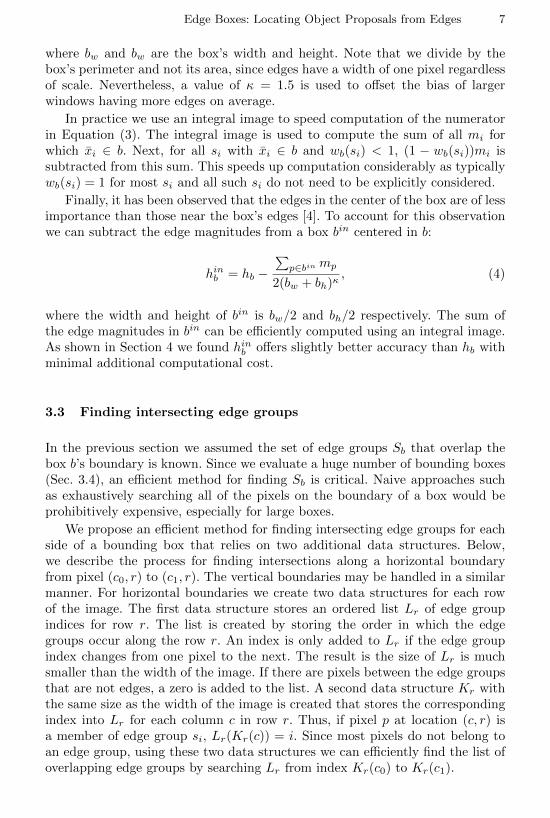
3.3 Finding intersecting edge groups

In the previous section we assumed the set of edge groups Sb that overlap thebox b’s boundary is known. Since we evaluate a huge number of bounding boxes(Sec. 3.4), an efficient method for finding Sb is critical. Naive approaches suchas exhaustively searching all of the pixels on the boundary of a box would beprohibitively expensive, especially for large boxes.

We propose an efficient method for finding intersecting edge groups for eachside of a bounding box that relies on two additional data structures. Below,we describe the process for finding intersections along a horizontal boundaryfrom pixel (c0, r) to (c1, r). The vertical boundaries may be handled in a similarmanner. For horizontal boundaries we create two data structures for each rowof the image. The first data structure stores an ordered list Lr of edge groupindices for row r. The list is created by storing the order in which the edgegroups occur along the row r. An index is only added to Lr if the edge groupindex changes from one pixel to the next. The result is the size of Lr is muchsmaller than the width of the image. If there are pixels between the edge groupsthat are not edges, a zero is added to the list. A second data structure Kr withthe same size as the width of the image is created that stores the correspondingindex into Lr for each column c in row r. Thus, if pixel p at location (c, r) isa member of edge group si, Lr(Kr(c)) = i. Since most pixels do not belong toan edge group, using these two data structures we can efficiently find the list ofoverlapping edge groups by searching Lr from index Kr(c0) to Kr(c1).


Fig. 2. An illustration of random bounding boxes with Intersection over Union (IoU)of 0.5, 0.7, and 0.9. An IoU of 0.7 provides a reasonable compromise between very loose(IoU of 0.5) and very strict (IoU of 0.9) overlap values.

3.4 Search strategy

When searching for object proposals, the object detection algorithm should betaken into consideration. Some detection algorithms may require object propos-als with high accuracy, while others are more tolerant of errors in bounding boxplacement. The accuracy of a bounding box is typically measured using the In-tersection over Union (IoU) metric. IoU computes the intersection of a candidatebox and the ground truth box divided by the area of their union. When eval-uating object detection algorithms, an IoU threshold of 0.5 is typically used todetermine whether a detection was correct [15]. However as shown in Figure 2,an IoU score of 0.5 is quite loose. Even if an object proposal is generated withan IoU of 0.5 with the ground truth, the detection algorithm may provide a lowscore. As a result, IoU scores of greater than 0.5 are generally desired.

In this section we describe an object proposal search strategy based on thedesired IoU, δ, for the detector. For high values of δ we generate a more con-centrated set of bounding boxes with higher density near areas that are likelyto contain an object. For lower values of δ the boxes can have higher diversity,since it is assumed the object detector can account for moderate errors in boxlocation. Thus, we provide a tradeoff between finding a smaller number of ob-jects with higher accuracy and a higher number of objects with less accuracy.Note that previous methods have an implicit bias for which δ they are designedfor, e.g. Objectness [4] and Randomized Prim [8] are tuned for low and high δ,respectively, whereas we provide explicit control over diversity versus accuracy.

We begin our search for candidate bounding boxes using a sliding windowsearch over position, scale and aspect ratio. The step size for each is determinedusing a single parameter α indicating the IoU for neighboring boxes. That is,the step sizes in translation, scale and aspect ratio are determined such that onestep results in neighboring boxes having an IoU of α. The scale values rangefrom a minimum box area of σ = 1000 pixels to the full image. The aspect ratiovaries from 1/τ to τ , where τ = 3 is used in practice. As we discuss in Section4, a value of α = 0.65 is ideal for most values of δ. However, if a highly accurateδ > 0.9 is required, α may be increased to 0.85.

After a sliding window search is performed, all bounding box locations witha score hinb above a small threshold are refined. Refinement is performed using


Fig. 3. Illustration of the computed score using (middle) and removing (right) contoursthat overlap the bounding box boundary. Notice the lack of clear peaks when thecontours are not removed. The magnitudes of the scores are normalized for viewing.The box dimensions used for generating the heatmaps are shown by the blue rectangles.

a greedy iterative search to maximize hinb over position, scale and aspect ratio.After each iteration, the search step is reduced in half. The search is halted oncethe translational step size is less than 2 pixels.

Once the candidate bounding boxes are refined, their maximum scores arerecorded and sorted. Our final stage performs Non-Maximal Suppression (NMS)of the sorted boxes. A box is removed if its IoU is more than β for a box withgreater score. We have found that in practice setting β = δ+ 0.05 achieves highaccuracy across all values of δ, Section 4.

4 Results

In this section we explore the performance and accuracy of our Edge Boxesalgorithm in comparison to other approaches. Following the experimental setupof previous approaches [7, 5, 8, 4] we evaluate our algorithm on the PASCAL VOC2007 dataset [15]. The dataset contains 9,963 images. All results on variants ofour approach are reported on the validation set and our results compared toother approaches are reported on the test set.

4.1 Approach variants

We begin by testing various variants of our approach on the validation set.Figure 4(a, b) illustrates the algorithm’s behavior based on the parameters αand β that control the step size of the sliding window search and the NMSthreshold, respectively, when generating 1000 object proposals.

As α is increased, the density of the sampling is increased, resulting in morecandidate boxes being evaluated and slower runtimes, Table 1. Notice that theresults for α = 0.65 are better than or nearly identical to α = 0.70 and α = 0.75.Thus, if a lower IoU value δ is desired α = 0.65 provides a nice accuracy vs.efficiency tradeoff. Depending on the desired IoU value of δ, the value of β maybe adjusted accordingly. A value of β = δ + 0.05 achieves high accuracy acrossall desired δ. As shown in Table 1, changes in β have minimal effect on runtime.


Fig. 4. A comparison of various variants of our approach. (a) The detection rate whenvarying the parameter α that varies the density of the sampling rate (default α = 0.65).(b) Results while varying the parameter β controlling the NMS threshold (defaultβ = 0.75). (c) The detection accuracy when various stages are removed from thealgorithm, including the removal of edges in the inner box, the bounding box loca-tion refinement, and the removal of the contours that overlap the box’s boundaries.(d) Detection accuracy when different edge detectors are used, including single-scaleStructured Edges [16] (default), multi-scale Structure Edges, and a fast variant thatruns at 10 fps without the edge sharpening enhancement introduced in [19]. Resultsusing the Canny edge detector [28] with varying amounts of blur are also shown.

Three useful variants of our algorithm are shown in Table 1; Edge Boxes 50,Edge Boxes 70, and Edge Boxes 90 that have settings for α and β adjusted forIoU thresholds of δ = 0.5, 0.7 and 0.9 respectively. For higher IoU thresholdsthat require extremely tight bounding boxes, α must be adjusted to search moredensely resulting in longer runtimes. Otherwise, α may be kept fixed.

Our second set of experiments tests several variants of the algorithm, Figure4(c, d). For these experiments we set δ to an intermediate value of 0.7 and showdetection rates when varying the number of object proposals. The primary con-tribution of our paper is that contours that overlap the bounding box’s boundaryshould be removed when computing the box’s score. Figure 4 shows that if thesecontours are not removed a significant drop in accuracy is observed. To gainintuition into the effect of the contour removal on the score, we illustrate thescore computed with and without contour removal in Figure 3. With contour


Table 1. Accuracy measures and runtimes for three variants of our algorithm: EdgeBoxes 50, Edge Boxes 70 and Edge Boxes 90. Accuracy measures include Area Underthe Curve (AUC) and proposal recall at 1000 proposals. Parameter values for α and βare shown. All other parameters are held constant.

removal the scores have strong peaks around clusters of edges that are morelikely to form objects given the current box’s size. Notice the strong peak withcontour removal in the bottom left-hand corner corresponding to the van. Whencontours are not removed strong responses are observed everywhere.

If the center edges are not removed, using hb instead of hinb , a small dropin accuracy is found. Not performing box location refinement results in a moresignificant drop in accuracy. The quality of the initial edge detector is also im-portant, Figure 4(d). If the initial edge map is generated using gradient-basedCanny edges [28] with varying blur instead of Structured Edges [16] the resultsdegrade. If multi-scale Structured Edges are computed instead of single-scaleedges there is a minimal gain in accuracy. Since single-scale edges can be com-puted more efficiently we use single-scale edges for all remaining experiments.The runtime of our baseline approach which utilizes single-scale edges is 0.25s.

If near real-time performance is desired, the parameters of the algorithmmay be adjusted to return up to 1000 boxes with only a minor loss in accuracy.Specifically, we can reduce α to 0.625, and increase the threshold used to de-termine which boxes to refine from 0.01 to 0.02. Finally, if we also disable thesharpening enhancement of the Structured Edge detector [19], the runtime ofour algorithm is 0.09s. As shown in Figure 4(d), this variant, called Edge BoxesFast, has nearly identical results when returning fewer than 1000 boxes.

4.2 Comparison with state-of-the-art

We compare our Edge Boxes algorithm against numerous state-of-the-art algo-rithms summarized in Table 2. Results of all competing methods were providedby Hosang et al. [26] in a standardized format. Figure 5 (top) shows the de-tection rates when varying the number of object proposals for different IoUthresholds. For each plot, we update our parameters based on the desired valueof δ using the parameters in Table 1. Edge Boxes performs well across all IoUvalues and for both a small and large number of candidates. Selective Search [5]achieves competitive accuracy, especially at higher IoU values and larger numberof boxes. CPMC [6] generates high quality proposals but produces relatively fewcandidates and is thus unable to achieve high recall. BING [11], which is veryfast, generates only very loosely fitting proposals and hence is only competi-


Fig. 5. Comparison of Edge Boxes to various state-of-the-algorithms, including Ob-jectness [4], Selective Search [5], Randomized Prim’s [8] and Rahtu [7]. The variationsof our algorithm are tested using δ = 0.5, 0.7 and 0.9 indicated by Edge Boxes 50, EdgeBoxes 70 and Edge Boxes 90. (top) The detection rate vs. the number of bounding boxproposals for various intersection over union thresholds. (bottom) The detection ratevs. intersection over union for various numbers of object proposals.

tive at low IoU. In contrast our approach achieves good results across a varietyof IoU thresholds and quantity of object proposals. In fact, as shown in Table2, to achieve a recall of 75% with an IoU of 0.7 requires 800 proposals usingEdge Boxes, 1400 proposals using Selective Search, and 3000 using RandomizedPrim’s. No other methods achieve 75% recall using even 5000 proposals. EdgeBoxes also achieves a significantly higher maximum recall (87%) and Area Underthe Curve (AUC = 0.46) as compared to all approaches except Selective Search.

Figure 5 (bottom) shows the detection rate when varying the IoU thresholdfor different numbers of proposals. Similar to Figure 4(a,b), these plots demon-strate that setting parameters based on δ, the desired IoU threshold, leads togood performance. No single algorithm or set of parameters is capable of achiev-ing superior performance across all IoU thresholds. However, Edge Boxes 70performs well over a wide range of IoU thresholds that are typically desired inpractice (IoU between 0.5 and 0.8, Figure 2). Segmentation based methods alongwith Edge Boxes 90 perform best at very high IoU values.

We compare the runtime and summary statistics of our approach to othermethods in Table 2. The runtimes for Edge Boxes includes the 0.1 seconds needed


AUC N@25% N@50% N@75% Recall Time

BING [11] .20 292 – – 29% .2s

Rantalankila [10] .23 184 584 – 68% 10s

Objectness [4] .27 27 – – 39% 3s

Rand. Prim’s [8] .35 42 349 3023 80% 1s

Rahtu [7] .37 29 307 – 70% 3s

Selective Search [5] .40 28 199 1434 87% 10s

CPMC [6] .41 15 111 – 65% 250s

Edge boxes 70 .46 12 108 800 87% .25s

Table 2. Results for our approach, Edge Boxes 70, compared to other methods forIoU threshold of 0.7. Methods are sorted by increasing Area Under the Curve (AUC).Additional metrics include the number of proposals needed to achieve 25%, 50% and75% recall and the maximum recall using 5000 boxes. Edge Boxes is best or near bestunder every metric. All method runtimes were obtained from [26].

to compute the initial edges. Table 2 shows that our approach is significantlyfaster and more accurate than previous approaches. The only methods withcomparable accuracy are Selective Search and CPMC, but these are considerablyslower. The only method with comparable speed is BING, but BING has theworst accuracy of all evaluated methods at IoU of 0.7.

Finally, qualitative results are shown in Figure 6. Many of the errors occurwith small or heavily occluded objects in the background of the images.

5 Discussion

In this paper we propose an effective method for finding object proposals inimages that relies on one simple observation: the number of edges that are whollyenclosed by a bounding box is indicative of the likelihood of the box containingan object. We describe a straightforward scoring function that computes theweighted sum of the edge strengths within a box minus those that are part ofa contour that straddles the box’s boundary. Using efficient data structures andsmart search strategies we can find object proposals rapidly. Results show bothimproved accuracy and increased efficiency over the state of the art.

One interesting direction for future work is using the edges to help generatesegmentation proposals in addition to the bounding box proposals for objects.Many edges are removed when scoring a candidate bounding box; the locationof these suppressed edges could provide useful information in generating seg-mentations. Finally we will work with Hosang at al. to add Edge Boxes to theirrecent survey and evaluation of object proposal methods [26] and we also hopeto evaluate our proposals coupled with state-of-the-art object detectors [13].

Source code for Edge Boxes will be made available online.


Fig. 6. Qualitative examples of our object proposals. Blue bounding boxes are theclosest produced object proposals to each ground truth bounding box. Ground truthbounding boxes are shown in green and red, with green indicating an object was foundand red indicating the object was not found. An IoU threshold of 0.7 was used todetermine correctness for all examples. Results are shown for Edge Boxes 70 with 1,000object proposals. At this setting our approach returns over 75% of object locations.

References

1. Viola, P.A., Jones, M.J.: Robust real-time face detection. IJCV 57(2) (2004)137–154

2. Dalal, N., Triggs, B.: Histograms of oriented gradients for human detection. In:CVPR. (2005)

3. Felzenszwalb, P., Girshick, R., McAllester, D., Ramanan, D.: Object detectionwith discriminatively trained part based models. PAMI 32(9) (2010) 1627–1645

4. Alexe, B., Deselaers, T., Ferrari, V.: Measuring the objectness of image windows.PAMI 34(11) (2012)

5. Uijlings, J.R.R., van de Sande, K.E.A., Gevers, T., Smeulders, A.W.M.: Selectivesearch for object recognition. IJCV (2013)


6. Carreira, J., Sminchisescu, C.: Cpmc: Automatic object segmentation using con-strained parametric min-cuts. PAMI 34(7) (2012)

7. Rahtu, E., Kannala, J., Blaschko, M.: Learning a category independent objectdetection cascade. In: ICCV. (2011)

8. Manen, S., Guillaumin, M., Van Gool, L., Leuven, K.: Prime object proposals withrandomized prims algorithm. In: ICCV. (2013)

9. Endres, I., Hoiem, D.: Category-independent object proposals with diverse ranking.PAMI (2014)

10. Rantalankila, P., Kannala, J., Rahtu, E.: Generating object segmentation proposalsusing global and local search. In: CVPR. (2014)

11. Cheng, M.M., Zhang, Z., Lin, W.Y., Torr, P.: BING: Binarized normed gradientsfor objectness estimation at 300fps. In: CVPR. (2014)

12. Wang, X., Yang, M., Zhu, S., Lin, Y.: Regionlets for generic object detection. In:ICCV. (2013)

13. Girshick, R.B., Donahue, J., Darrell, T., Malik, J.: Rich feature hierarchies foraccurate object detection and semantic segmentation. In: CVPR. (2014)

14. Deng, J., Dong, W., Socher, R., Li, L.J., Li, K., Fei-Fei, L.: Imagenet: A large-scalehierarchical image database. In: CVPR. (2009)

15. Everingham, M., Van Gool, L., Williams, C.K.I., Winn, J., Zisserman, A.: Thepascal visual object classes (voc) challenge. IJCV 88(2) (2010) 303–338

16. Dollar, P., Zitnick, C.L.: Structured forests for fast edge detection. In: ICCV.(2013)

17. Marr, D.: Vision: A computational investigation into the human representationand processing of visual information. Inc., New York, NY (1982)

18. Eitz, M., Hays, J., Alexa, M.: How do humans sketch objects? ACM TransactionsGraphics 31(4) (2012)

19. Dollar, P., Zitnick, C.L.: Fast edge detection using structured forests. CoRRabs/1406.5549 (2014)

20. Deselaers, T., Alexe, B., Ferrari, V.: Localizing objects while learning their ap-pearance. In: ECCV. (2010)

21. Siva, P., Xiang, T.: Weakly supervised object detector learning with model driftdetection. In: ICCV. (2011)

22. Gu, C., Lim, J.J., Arbelaez, P., Malik, J.: Recognition using regions. In: CVPR.(2009)

23. Hoiem, D., Efros, A.A., Hebert, M.: Geometric context from a single image. In:ICCV. (2005)

24. Russell, B.C., Freeman, W.T., Efros, A.A., Sivic, J., Zisserman, A.: Using multiplesegmentations to discover objects and their extent in image collections. In: CVPR.(2006)

25. Malisiewicz, T., Efros, A.A.: Improving spatial support for objects via multiplesegmentations. In: BMVC. (2007)

26. Hosang, J., Benenson, R., Schiele, B.: How good are detection proposals, really?In: BMVC. (2014)

27. Felzenszwalb, P.F., Huttenlocher, D.P.: Efficient graph-based image segmentation.IJCV 59(2) (2004)

28. Canny, J.: A computational approach to edge detection. PAMI (6) (1986) 679–698

edge boxes: locating object proposals from...

Documents