economic competition and the production of winning …
TRANSCRIPT
ECONOMIC COMPETITION AND THE PRODUCTION OF WINNING IN
PROFESSIONAL SPORTS
By
KEVIN P. MONGEON
A dissertation submitted in partial fulfillment of
the requirements for the degree of
DOCTOR OF PHILOSOPHY
WASHINGTON STATE UNIVERSITY School of Economic Sciences
MAY 2010
© Copyright by Kevin P. Mongeon, 2010
All Rights Reserved

© Copyright by KEVIN P. MONGEON 2010
All Rights Reserved

ii
To the Faculty of Washington State University:
The members of the Committee appointed to examine the dissertation
of KEVIN P. MONGEON find it satisfactory and recommend that it be
accepted.
___________________________________
Jill J. McCluskey, Ph.D., Chair
___________________________________
Jason Winfree, Ph.D.
___________________________________
Tom Marsh, Ph.D.
___________________________________
Robert Rosenman, Ph.D.

iii
ACKNOWLEDGMENTS
I consider myself to be most fortunate to have benefited from the teachings,
kindnesses, and advice of the very best. I sincerely thank the entire faculty and staff of
the School of Economic Sciences at Washington State University and in particular my
committee members. Dr. Jason Winfree, your patience in answering questions and
diligence in guiding me to do useful research is appreciated. Dr. Tom Marsh, I admire
your kindness, professionalism and deep thinking. Dr. Robby Rosenman, you have made
me a better economist and thinker and have guided me to become a professional. Dr. Jill
McCluskey, you let me find my passion and encourage me in every moment. For this I
am grateful beyond words. Very simply, I am a better person because of each of you.
To my friend Mike Boyle, my appreciation for your time and energy pales in
comparison to my appreciation for your friendship. You have my respect and I am
looking forward to more rich times. Thank you to my family: mom, dad, Heather, and
Murray, who have always been present and unconditionally supportive.

iv
ECONOMIC COMPETITION AND THE PRODUCTION OF WINNING IN
PROFESSIONAL SPORTS
Abstract
by Kevin P. Mongeon, Ph.D.
Washington State University
May 2010
Chair: Jill J. McCluskey
This dissertation includes three essays on the economics and management of
professional sports with an emphasis on strategic management and quantitative methods.
The first paper is a theoretical paper that provides an alternative perspective of
professional sports team owners’ incentive to invest in a level of talent. The second
paper examines the relationship between the demand for watching games on television
and attending games in person. The third paper is an application of microeconomic
theory and econometrics that estimates different forms of the contest success function and
develops a new empirical approach to measuring players’ effectiveness.
The chapter titled “Economic Competition and Player Investment in Sports
Leagues” provides an alternative perspective of professional sports teams’ incentives to
invest in talent based on market and ownership structures. Since territorial rights limit
fans’ ability to trade off between the qualities of teams that are direct substitutes, the
v
possibility exists that some fans will choose between indirect substitutes based on relative
team qualities (e.g. winning). If this is the case, then both the market and ownership
structures will affect the owner’s incentive to invest in talent. The condition of cross-
ownership decreases an owner’s incentive to invest in talent compared to the duopoly.
The chapter titled “A Comparison of Television and Gate Demand in the
National Basketball League” estimates the demand for gate attendance and television
audiences in the NBA and finds that the fans who attend games in person are inherently
different from fans who watch games on television. Fans who watch the games on
television are more responsive to winning and do not substitute for other professional
sport leagues compared to fans who attend the games in person.
The chapter titled “Contest Success Functions and Marginal Products of
Talent” contributes to the literature by being one of the first papers to empirically
estimate a contest success function. Although tournaments, conflicts, rent-seeking, and
sporting events have been modeled with contest success functions, little empirical support
exists. The contest success function is further used to determine the contribution to
winning of the candidate players for the 2010 Canadian Men’s Olympic Hockey Team.

vi
TABLE OF CONTENTS
ACKNOWLEDGMENTS iii
ECONOMIC COMPETITION AND THE PRODUCTION OF WINNING IN
PROFESSIONAL SPORTS iv
Abstract iv
CHAPTER 1: INTRODUCTION 1
Economic Competition and the Effects of Fan Loyalty on Team Quality 2
The Effects of Cross-Ownership on Team Quality 2
The Effects of League Policies on the Quality of Teams in Other Leagues 3
The Difference of Economic Competition and Winning between Gate and Television
Demand 3
The Production of Winning 4
The Marginal Product of Talent 5
Dissertation Format and Content 5
References 7
Figures 8
CHAPTER 2: ECONOMIC COMPETITION AND PLAYER INVESTMENT IN
SPORTS LEAGUES 9
Abstract 9
Introduction 10
Section II: A Two League – Two Team Model 14
Case 1: The Monopoly Case 15
Case 2: The Duopoly Case: Economic Competition 16

vii
The Effects of Fan Loyalty on Team Quality 18
The Effects of Economics Competition on Team Quality 19
The Effects of Strategic Competition on Team Quality 21
Case 4: Cross-ownership 23
The Effects of Cross-Ownership on Team Quality 23
Section III: The Impact of League Policies on Quality of Teams in Other Leagues 25
The Effects of Revenue Sharing on the Quality of Teams in Other Leagues 28
The Effects of Revenue Sharing with Cross-Ownership on the Quality of Teams in
Other Leagues 30
Section IV: An Example 33
Section V: Conclusions 35
References 37
Tables and Figures 39
Appendix A: Derivations of Theoretical Equations 43
CHAPTER 3: A COMPARISON OF TELEVISION AND GATE DEMAND IN THE
NATIONAL BASKETBALL ASSOCIATION 53
Abstract 53
Introduction 54
Data and Empirical Estimation 56
Empirical Results 58
Conclusion 62
References 63
Tables 66

viii
CHAPTER 4: CONTEST SUCCESS FUNCTIONS AND MARGINAL PRODUCT OF
TALENT 68
Abstract 68
INTRODUCTION 69
The Model 71
Empirical Estimation 74
Empirical Results from Stage 1 and 2 76
Empirical Results of Stage 3: The Contest Success Function 79
CSF Regression Diagnostics 81
Classification Tables 82
Goodness-of-fit 83
The Marginal Product of Talent and Contribution to Winning 86
An Example: The 2010 Canadian Men’s Olympic Hockey Team 86
Concluding Comments 91
REFERENCES 93
TABLES AND FIGURES 96

1
CHAPTER 1: INTRODUCTION
Since Rottenberg’s (1954) seminal article spurred the development of the field of
research called sports economics, winning has been recognized as an important
determinant of demand. However, the market for professional sports has changed.
Economic competition exists more than before. Leagues have expanded to include more
teams. From 1970 to 2010 membership in Major League Baseball (MLB), the National
Basketball Association (NBA), and the National Hockey League (NHL) increased from
24, 17, and 14 respectively to 30. In the absence of direct competition, this expansion has
increased the amount of indirect competition from teams in competing leagues.
Therefore, examining the impact of substitutability between teams in different leagues
and winning is of increasing importance.
The dissertation focuses on the impact of the substitution effect between teams in
different leagues and the production of winning. Some of the questions investigated are:
What are the impacts of economic competition and ownership structures on team quality?
Under what conditions do league policies affect the quality of teams in other leagues?
How do economic competition and winning affect gate demand differently than
television demand? Finally, how can the production of winning be modeled? The
answers to these questions provide insights into league behavior and factors that
determine demand beyond the current literature.
2
Economic Competition and the Effects of Fan Loyalty on Team Quality
Sports teams operate with regional monopoly. Fort and Quirk (1995) introduced
a two team league model to analyze owners’ incentives to invest in winning. However,
the absence of direct competition has created a “gap in the chain of substitutes”
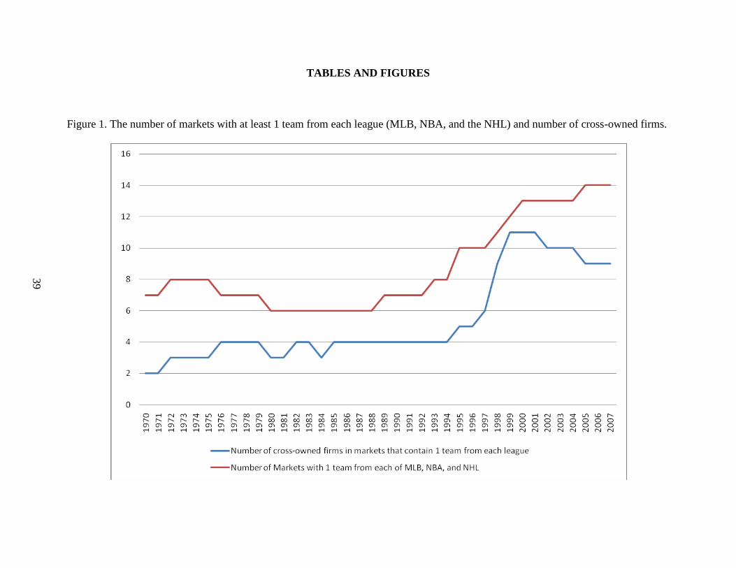
introducing product dimensions into the market space. Figure 1 depicts the number of
markets with at least one team from each league (MLB, NBA, and NHL). Using the
number of markets with one team from each of the three leagues as a benchmark for the
amount of economic competition, the number of markets with one team from each of the
three leagues increased from 7 to 14. Chapter Two shows that, if fans make consumption
choices based on the quality of all the teams in the market, then teams with more loyal
fans will have lower quality teams.
The Effects of Cross-Ownership on Team Quality
Cross-ownership is the common ownership of teams in different leagues located
in the same region. Winfree (2008) shows that teams in competing leagues are
substitutes. Figure 1 also graphs the number of cross-owned firms among the markets
that contain one team from each of the three leagues. As the number of markets with a
team from each league increased from 7 to 14, the number of cross-owned firms
increased from 2 to 9, obtaining a maximum of 11. From an owner’s perspective, an
important advantage of the cross-owned firm is: in solving the joint profit maximization
problem, it eliminates the externalities between the teams. Therefore, the cross-owned
firm mitigates the effects of economic competition. Chapter Two shows that the cross-
owned firm will invest less in talent than the duopolist.

3
The Effects of League Policies on the Quality of Teams in Other Leagues
A considerable body of research studies the effects of these league policies on the
winning percentages of teams within their own leagues. Salary caps improve competitive
balance by forcing the amount that large market owners invest in talent below their profit
maximizing level (Fort and Quirk (1995), Vroomam (1995)). Depending on the
assumptions of the model, the effects of revenue sharing on competitive balance are
different. Assuming a fixed supply of talent, Fort and Quirk (1995) show that revenue
sharing results in no change in competitive balance. Assuming perfectly elastic supply of
talent, Syzmanki (2004) shows that revenue sharing worsens competitive balance. In
contrast to previous work, I examine how a salary cap and revenue sharing affect the
quality of teams in other leagues. In this analysis, the qualities of teams in leagues are
linked. Therefore, league polices can affect the quality of teams in other leagues.
Chapter Two derives series of conditions in which salary caps and revenue sharing will
increase or decrease the talent levels in other leagues.
The Difference of Economic Competition and Winning between Gate and Television
Demand
While historical television revenue data are not widely available, it is accepted
that revenues generated from television have increased. For the 2007-08 season, the
NBA received $4.6 billion from league-wide contracts with ABC/ESPN and AOL/Time
Warner. Although media revenue is a growing source of income for sports teams, little
is known about the factors of demand for games on television. Much of the literature on

4
the demand for sports television has focused on the substitution between watching a
game on television and watching a game live. Chapter three compares the differences in
the substitution effect between direct and indirect substitutes as well as the effects of
winning for both television and gate demand in the NBA. The results show that fans
watching television are an entirely different group than fans who attend games. Fans
who watch the games on television are more price sensitive, demand more winning, and
do not substitute for other professional sports, compared to fans who attend games.
The Production of Winning
A contest is a game in which players increase the probability of winning by
exerting effort with the objective of obtaining a prize (Skaperdas, 1996). Although
sporting events, tournaments, conflicts, and rent-seeking have been modeled with CSFs,
little empirical support exists. Although the literature on CSFs is extensive, only Hwang
(2009) has performed an empirical analysis. In the sports economics literature, Fort and
Winfree (2009), Rascher (1987), Szymanski (2003, 2004), Szymanski and Kesenne
(2004), and Kesenne (2005, 2006) have used CSFs in the modeling of leagues, but
empirical analysis using sports data is absent from the literature. In Chapter 4, I use a
multi-stage regression technique to estimate and compare two popular forms of the CSF,
the ratio and difference forms. Results show that the ratio form of the CSF is a better fit
for the data. The estimate of talent parameter in the ratio form is one. This supports the
assumption made by most sports economists.

5
The Marginal Product of Talent
Scully (1974) was the first to estimate the marginal product of talent. Although
others (Scully (1989), Zimbalist, (1992)) have extended Scully’s 1974 work, none have
fundamentally changed or improved the method of determining the marginal product of
talent. Without imposing a model, Scully and others used season level data in their
analysis. Season level data is attractive for analysis. It is easily understood because the
information the data contains is smoothed out from averaging, although it still contains
systematic error. In comparison, contest level data is difficult to interpret. However, by
imposing a model, the systematic error contained in the data is eliminated. In Chapter 4,
I use contest level data and the ratio form of the CSF to estimate the marginal product of
talent for the candidate players of the 2010 Canadian Men’s Olympic Hockey Team.
Dissertation Format and Content
This dissertation contains three articles. The first article (Chapter 2) contains
three sections of analysis. The first section of analysis develops a two-team/two-league
model of professional sports leagues. While previous literature focuses on the regional
monopoly power in professional sports, the scope of this research is broader. The model
is first derived using the monopoly setting. Then, the cases of economic competition and
cross-ownership are analyzed and compared. A measurement of fan loyalty is derived
from the model and the implications of fan loyalty on team quality are discussed. The
second section of analysis models the effects that salary caps and revenue sharing have
on the quality of teams in other leagues. This paper is the first in the literature to analyze

6
the cross-league effects of league policies. The third section of analysis works through
an example using functional forms.
The second article (Chapter 3) contributes to the sports economics literature by
comparing the factors that contribute to gate and television demand in the NBA.
Historically, gate demand has been analyzed. However, although television revenues
have increased, analysis of factors that contribute to demand for fans who watch games
on television is limited. To estimate demand, I use two empirical models. Each is a
linear regression model. The first model includes time effects, and the second includes
both time and team effects.
The third article (Chapter 4) contributes to the CSF and sports economics
literatures. This paper contributes to the CSF literature by being one of the first papers to
empirically estimate CSFs and provide support for a particular form. This paper
contributes to the sports economics literature by using contest success function to
improve on the methodology of determining the marginal product of talent. The
difference and ratio forms of CSFs have been identified by researchers as popular choices
to develop theoretical properties and model tournaments, conflicts, rent-seeking, and
sports leagues. Furthermore, sports economists often use a simplified version of the ratio
form with no empirical justification. In this article, I use a multi-stage regression to
estimate the parameters of difference and ratio forms of the CSFs and then compare the
forms for best fit using various criteria. Empirical estimation of the CSF places value on
the inputs that contribute to winning. Therefore, I develop formulas to calculate the
marginal product of talent for hockey players.
7
REFERENCES
Fort, R. and Quirk, J. (1995). Cross-Subsidization, Incentives, and Outcomes in
Professional Team Sports Leagues. Journal of Economic Literature 33(3):1265-
1299.
Fort, R. and Winfree, J. (2009). Sports Really are Different: The Contest Success
Function and the Supply of Talent. Review of Industrial Organization 34(1):69-
80.
Hwang, S. (2009). Contest Success Functions: Theory and Evidence. Working Paper.
Kesenne, S. (2005). Revenue sharing and competitive balance: Does the invariance
proposition hold? Journal of Sports Economics 5:98-106.
Kesenne, S. (2006). The win maximization model reconsidered: Flexible talent supply
and efficiency wages. Journal of Sports Economics 7:416–427.
Rottenberg, S (1956). The Baseball Players' Labor Market. The Journal of Political
Economy 64(3):242-258.
Racher, D. (1997). A model of professional sports leagues. In: W. Hendricks (Ed.),
Advances in the Economics of Sport, volume 2:27-76.
Scully, G.W. (1974). Pay and Performance in Major League Baseball. American
Economic Review 64:915-930.
Skaperdas, S. (1996) Contest Success Functions. Economic Theory 7(2):283-290.
Szymanski, S. (2004). Professional team sports are only a game: The Walrasian fixed-
supply conjecture model, contest-Nash equilibrium, and the invariance principle.
Journal of Sports Economics 5:111-126.
Szymanski, S. and Késenne, S. (2004) Competitive balance and gate revenue sharing in
team sports. Journal of Industrial Economics 52(1):165-177.
Vrooman, J. (1995). A General Theory of Professional Sports Leagues. Southern
Economic Journal 61(4):971-990.
Winfree, J. (2008). Owners incentives during the 2004-05 National Hockey League
lockout. Journal of Applied Economics 41(25):3275-3285.
Zimbalist, A. (1992). Baseball and Billion. New York: Basic Books.

8
FIGURES
Figure 1. The number of markets with at least 1 team from each league (MLB, NBA, and
the NHL) and number of cross-owned firms.

9
CHAPTER 2: ECONOMIC COMPETITION AND PLAYER INVESTMENT IN
SPORTS LEAGUES
Abstract
Although most direct competition has been eliminated, indirect competition exists
between teams in the same region but in different professional sports leagues. If fans
make consumption choices for team products based on the quality of all teams (across
sports) that are present in their region, then economic competition and ownership
structure can impact the quality of teams. This article constructs a professional sports
league model of an owner’s incentive to invest in talent in the presence of competition
from other sports leagues. Consumer preferences are allowed to vary across sports, and
the winning percentages of teams in other leagues affect demand. The results suggest
that more loyal fans reduce the incentive to invest in talent, cross-ownership decreases an
owner’s incentive to invest in talent, and that one’s league policies can have an effect on
the quality of teams in other leagues.

10
INTRODUCTION
Operating as cartels, professional sports leagues have empowered their teams with
regional monopoly power. However, this absence of direct competition has created a
“gap in the chain of substitutes” introducing product dimensions into the market space. It
is conceivable that fans make consumption choices based on the quality of all teams
(across sports) that are present in their region. In this article, I investigate how economic
competition between teams in alternative sports leagues can affect quality of teams, as
well as how the ownership structure can decrease team quality. The analysis is then
extended to analyze the effects that revenue sharing and salary caps can have on the
quality of teams in other leagues.
Higher levels of team quality, represented by winning percentage, can increase
demand for the team’s products (e.g. tickets, television broadcast rights, and
merchandise). If fans enjoy many sports and obtain utility from rooting for a winning
team, then it raises a number of research questions. How does economic competition
from professional teams in other sports affect an owner’s incentive to invest in talent?
What are the conditions in which the winning percentages between teams act as strategic
compliments or substitutes? How does owning teams in different leagues that are located
in the same market (hereafter called cross-ownership) alter an owner’s incentive to invest
in talent? How will a salary cap and revenue sharing affect the quality of teams in other
leagues? Extending the work of El Hodiri and Quirk (1971) and Quirk and El Hodiri
(1974), I develop a model of an owner’s incentive to invest in talent in the presence of
competition from other sports leagues. I allow consumer preferences to vary across
sports, and the winning percentage of teams in other leagues to affect demand. Our
11
analysis highlights that cross-ownership decreases an owner’s incentive to invest in talent
and that one’s league policies can have an effect on the quality of teams in other leagues.
Traditionally, sports leagues are modeled as monopolies with talent as a long-run
choice variable in the team’s profit maximization problem (Fort and Winfree, 2009).
First, I model the monopoly case in which the owner considers the winning percent of the
teams from other leagues in the market into their objective function. Depending on its
own-revenue elasticity of winning, the monopolist will either invest in high or low levels
of talent. This is the point where Fort (1995) and others created the two-team model,
used the adding-up of winning percentage constraint to find an equilibrium winning
percentage, and analyzed the effects of league policies. In contrast, I use the first-order
conditions to compare the owner’s incentive to invest in talent across three types of
markets: monopoly, competitive, and cross-ownership.
Second, I model economic competition. Markets with multiple teams and
heterogeneous fan preferences yield different results. Figure 1 depicts the number of
markets with more than one major league team. Using National Hockey League (NHL),
National Basketball Association (NBA), and Major League Baseball (MLB) as a
benchmark, the number of markets with one team from each of the three leagues
increased from 7 to 14 from 1970 to 2007. With the presence of another team in the
market, I incorporate sports fans’ preferences for winning in the market into the model.
Overall, if fans are loyal1, owners will invest a lower amount in talent. Consider the
following example: a sports fan who likes hockey and basketball prefers to watch a
1 Loyal fans are fans who do not readily switch between teams based on winning percentages. A formal
definition is presented later in the paper.

12
hockey team with a winning percentage of 0.400 compared to a basketball team that has a
winning percentage of 0.550. However, the same fan may prefer the basketball team if it
were to have a 0.650 winning percentage, all else constant. This situation forces owners
to consider fans’ substitution based on the winning percentages of teams in other sports
leagues into their decisions to invest in talent.
Third, I model the effects of cross-ownership and find that the cross-ownership
results in lower investment in talent compared to markets in which economic competition
exists. The study of cross-ownership is important because it is present in the
marketplace. Table 1 shows the cross-ownership among MLB, NBA, and NHL teams.
To show the relationship between the amount of indirect competition and cross-
ownership, Figure 1 also graphs the number of cross-owned firms among the markets that
contain one team from each of the three leagues. As the number of markets with a team
from each league increased from 7 to 14, the number of cross-owned firms increased
from 2 to 9, obtaining a maximum of 11 in 1999, 2000, and 2001. The correlation
coefficient is 0.91. Table 2 is a summary of the cross-ownership among markets that
contained at least one team from each of the three leagues from 1950 to present. Ten of
the eleven markets have had ownership groups that owned teams in competing leagues.
Of the regions that have contained at least one team from each league, Minneapolis is the
only city that has not had cross-owned teams2. I summarize the progression of cross-
ownership in Appendix C.
Cross-ownership has its other implications: pricing and cost efficiencies.
Depending on the heterogeneity of the products, a cross-owned firm has the incentive to
2 Minneapolis lost their NHL team to Dallas in 1993 before recently gaining back another team from
expansion franchise in 2000.

13
increase or decrease ticket prices accordingly. Winfree (2008) shows that because of the
substitutability between teams in competing leagues, cross-ownership can lengthen the
duration of work-stoppages.
Consequently, the 2004-05 NHL work-stoppage resulted in a revenue increase of
approximately $53 million for teams in competing leagues that were owned by a common
firm. In addition, if the prices are substitutes, the increased price could allow the not
otherwise successful team to become viable when it is not socially optimal, creating an
overprovision of teams. Furthermore, the potential for cost saving exists if the cross-
owned firm’s cost function is not separable. Shared stadiums or television broadcasting
might be examples of non-separable costs. To the best of the author’s knowledge, the
overprovision of teams and the structure of the cost functions have not been studied in the
sports literature. Both are beyond the scope of this article.
Finally, I study the effects of revenue sharing and salary caps on the talent levels
in other leagues. A considerable body of research studies the effects of these cross-
subsidization techniques on the winning percentages of teams within their own leagues.
Salary caps improve competitive balance by forcing the amount that large market owners
invest in talent below their profit maximizing level (Fort and Quirk (1995), Vroomam
(1995)). Depending on the assumptions of the model, the effects of revenue sharing on
competitive balance are different. A fixed supply of talent results in no change to
competitive balance while perfectly elastic supply of talent worsens competitive balance
(Fort and Quirk (1995), Syzmanki (2004)). Kesenne (2000) shows that competitive
balance can be improved with revenue sharing if revenue is a function of both the home
and away teams’ winning percents. In contrast to previous work, I examine how a salary

14
cap and revenue sharing affect the quality of teams in other leagues. As a consequence, I
investigate the implications of the policies of other leagues. In our analysis, leagues are
inherently linked and, therefore, league polices can affect the quality of teams in other
leagues. I derive a series of conditions in which salary caps and revenue sharing will
increase or decrease the talent levels in other leagues.
The rest of the article proceeds as follows: section II sets up team models and
compares the different incentive for owners to invest in talent across different cases:
monopoly, economic competition, and cross-ownership. Section III determines the
impact of league policies in alternate leagues, and section IV is an example with
functional forms. Section V is the conclusion and discusses some implications.
Section II: A Two League – Two Team Model
Consider a product market in which some fans’ tastes are diverse, so that there are
two groups of fans: sport-specific fans and sports fans. Sport-specific fans only consume
a specific sport and their purchasing decisions are based entirely on the quality of that
specific team, regardless of the presence of a competing team in the market. In contrast,
sports fans will potentially consume any sport that is in the market and their consumption
choice depends on the quality of all of the teams in the market. I assume that teams are
completely uninformed about whether any particular fan is a sport-specific fan or a sports
fan. Therefore, teams only know the proportion of total fans relative to the monopoly
case.
I assume there are two leagues and two teams in each league. The general model
assumptions are: ,i j is the profit for the team in league or i a b (e.g. NBA, or NHL)

15
and market 1, 2, or 3j (e.g. New York, Edmonton, Seattle). Market 1 is considered to
be the large revenue potential market and markets 2 and 3 are small revenue potential
markets. Further, for the purposes of this paper, league a is located in markets 1 and 2
and league b is located in markets 1 and 3. R is the team’s revenue. Revenue is a
function of its own team’s winning percentage, w . Winning percentage is a function of
talent or investment in talent, t , of both teams in the league The function (gamma)
represents the proportion of total fans relative to the monopoly case. It is an open
bounded set between zero and one. Gamma is a function of the winning percentages of
both teams in the market3. Therefore, R represents revenue normalized to the
monopolist. To recap, is a function of the winning percentages of teams across
leagues, and w is a function of talent within the same league. Fans attend either team
i a or i b in market j , not both4. Next, I model a firm operating in three different
economic markets (monopoly, duopoly, and cross-ownership) and compare the owner’s
incentive to invest in talent across cases.
Case 1: The Monopoly Case
With the absence of indirect competition, I normalize the monopolist’s proportion
of total fans to one. Therefore the monopolist’s normalized revenue is derived as
follows: ,1 ,1 ,1 ,1 ,1 ,1 ,1 ,1 ,1 ,1 ,1( , ) ( ) ( ) ( ) ( )a a b a a a a a a a aw w R w w R w R w . Therefore, the profit
function for team a in market 1 is,
3 Hereafter I refer to the proportion of total fans relative to the monopoly case as the proportion of total
fans. 4 To focus on quality, I am holding quantity constant and therefore modeling profit as a function of revenue
or price.
16
1 1 1 1a a a aR w t (1)
To ensure positive but decreasing marginal revenue of investment in talent on
revenue, I assume the usual conditions of,
,1
,1
0a
a
R
t
,
2
1
1 1
0a
a a
R
t t
(2)
The first order condition is,
1 1 1
1 1 1
1a a a
a a a
w dR
t t dw
(3)
Equation (3) implies that the firm will invest in talent to the point where the contribution
to talent on revenue equals the cost of talent. I will compare equation (3) with first-order
conditions of the duopolist and cross-owned firm.
Case 2: The Duopoly Case: Economic Competition
To illustrate the effects of indirect competition, consider the market entry of an
economic competitor from a different league, creating a duopoly. Consequently, the
proportion of total fans is a function of the winning percentages of both teams that are
present in the market. Notationally, this is represented by the function,1 ,1 ,1( , )a a bw w .
With the presence of another team in the market, both the preferences of sport-specific
fans and sports fans are incorporated into the model. No change will occur with regards
to the behavior of sport-specific fans. Sport-specific fans will only choose to attend a
specific sport regardless of the winning percentage of the other team in the market. The
indirect competition provides a choice for sports fans. Sports fans’ consumption choice
depends on winning percentages of both teams in the market.

17
I assume that a team’s own winning percentage does not decrease its proportion
of the potential fan base and the other team’s winning percent does not increase it; that is,
1
1
0a
aw
and 1
1
0a
bw
. The profit function for the duopolist is
1 1 1 1 1 1 1,a a a b a a aw w R w t (4)
The first order condition is,
1 1 1 11 1
1 1 1 1
1a a a aa a
a a a a
w dRR
t t w dw
(5)
The marginal revenue from winning, 1
1
a
a
dR
dw, that was present the monopolist’s first order
condition is divided into two parts: 1 11 1
1 1
and a aa a
a a
dRR
w dw
. The product 1
1
1
aa
a
Rw
is the
revenue gained from the additional fans (both sports fans and sport-specific fans) that
attend the game due to a one-unit increase in the team’s own winning percentage, holding
the effects of winning on revenue constant. The product 11
1
aa
a
dR
dw is the additional
normalized revenue generated from a one-unit increase in winning percentage, holding
the effects of winning on the proportion of total fans constant. The sum of the two
products, 1 11 1
1 1
a aa a
a a
dRR
w dw
, represents a more flexible form of the marginal revenue
than the monopolist’s. If 1 and 1
1
0a
aw
then equation (5) is equivalent to equation
(3). This is the assumption made by other researchers. The assumption implies that
winning does not cause an increase in the proportion of total fans and the market
consisted of only sport a specific fans. This does not imply that there cannot be another

18
sport b in the market. Rather there are simply no fans of sport a
and sport b . If 0 ,
it implies that the market consists of only sport b specific fans, leaving team a with no
potential fan base. For any 1 , the proportion of total fans has decreased because some
sports fans are attending sport b . An example of this might be if fans substitute their
season tickets for the existing team with season tickets of the economic competitor
entering the market.
The Effects of Fan Loyalty on Team Quality
I begin my analysis by introducing a definition of loyalty from the marketing
literature. Generally, loyalty is defined as repeat purchasing frequency or same-brand
purchasing (Oliver, 1999). Recall, 1
1
a
aw
represents the increase in the proportion of total
fans from a one-unit increase in winning percentage. Therefore high (low) values of
1
1
a
aw
imply sports fans are sensitive (insensitive) to the winning percentage of team a .
Therefore, greater (lesser) values of 1
1
a
aw
imply fans are less (more) loyal. I summarize
the effects of fan loyalty on team quality in the following proposition.
Proposition 1: If fans are more loyal fans, then owners will invest less in talent.
Proof: Directly from equation (5).
19
The Effects of Economics Competition on Team Quality
To analyze the effect of economic competition, I compare equation (5) with
equation (3). If 1
1
0a
aw
, then the proportion of total fans is not sensitive to increases in
team 'a s winning percentage and equation (3) simplifies to
1 11
1 1
1a aa
a a
dR w
dw t
(6).
If in addition to 1
1
0a
aw
, 1 , equation (6) is less than equation (3), showing
that the team will invest less in talent compared to the monopoly case. This is because
the competing team makes the potential fan base smaller by reducing their effect
population. However, if 1
1
0a
aw
, then the proportion to total fans is sensitive to team
'a s winning percentage. Therefore the duopolist’s level of investment in talent
compared to the monopolist is ambiguous. I summarize the relationship with the
following proposition.
Proposition 2: A duopolist owner will invest more in talent compared to a monopolist if
the normalized revenue from a 1% increase in winning on the proportion of fans is
greater than the reduction in revenue compared to the monopolist from a 1% increase in
winning on revenue due to the smaller fan base.
1 1, ,1 1 1a aw r wa aR R (7)
Proof: See Appendix A
20
The function ,w is the winning percentage elasticity of the proportion of fans and
,r w is the winning percentage elasticity of revenue. Since represents the proportion of
fans relative to the monopoly case, 1 represents the reduction in the proportion due
to the team that entered the market56
. The left hand side (LHS) of equation (7) is the
increase in the normalized revenue from a 1% increase in winning on the proportion of
fans. The right hand side (RHS) of equation (7) is the reduction in revenue compared to
the monopolist from a 1% increase in winning on revenue due to the smaller fan base. It
is useful to think of R and 1 R as weights representing the importance of the
respected elasticity.
If the team entering the market altered the fan base in such a way that the fan base
was evenly split, then .5 and equation (7) simplifies to , ,w r w . This implies that
the duopolist would invest more into talent if the team can gain more fans by winning
than the additional revenue gained from that win. This is because the marginal revenue
of winning is less for the duopolist than the monopolist due to the small fan base, holding
the effect of winning on the proportion of fans constant. Further, less loyal fans (high
values of ,w ) result in the condition equation (7) to be more easily satisfied, resulting in
greater investment in talent compared to the monopolist. However, if the winning
elasticity of revenue ,r w is high, the condition in equation (7) will be less easily
satisfied because the increases in winning percentage will result in the monopolist
5 Although 1 'aR s divide out they are included to make easier comparisons later in the paper.
6
1 1
1 1
,a a
a a
w
w
w
and 1 1
1 1
,a a
a a
r w
R w
w R

21
gaining more revenue than the duopolist by the factor equivalent to the reduction in total
fans, 11 a .
The Effects of Strategic Competition on Team Quality
Once a duopoly is established, teams have the opportunity to make strategic
investments in talent. I take the approach outlined by Dixit (1987) with teams choosing
levels of talent without pre-commitment. The strategic effect of talent on the changes in
the other team’s (team b ) talent is determined by further differentiating equation (5) as
follows,
2 2
1 1 1 1 1 11
1 1 1 1 1 1 1 1
a a b a a aa
a b a b a b b a
w w dRR
t t t t w w w dw
(8)
The sign of equation (8) is ambiguous. Equation (8) introduces a new term,
2
1
1 1
a
a bw w
,
the strategic effect of winning percentages on the proportion of fans. Little can be said
about the sign of magnitude of
2
1
1 1
a
a bw w
without a functional form
78. The product
2
11
1 1
aa
a b
Rw w
, represents the increase or decrease in revenue due to strategic effects of
7 If the logistic form were imposed on
2
1
1 1
a
a bw w
then,
2
1
1 1
0a
a bw w
if and only if
,1 ,1a bf f . See the
non-symmetric case by Dixit (1987) for a graphical representation of the strategic effects. Here the logistic
function is specified as ,1
,1
,1 .1
( )
( ) ( )
a
a
a b
f w
f w f w
and
2 ' '
,1 ,1 ,1 ,1 ,1
3
,1 ,1 ,1 ,1
( )
( )
a a b a b
a b a b
d f f f f
dw dw f f
8 The logistic function is a natural choice for a discrete model (see McFadden, 1973) and is used
extensively in the contest theory literature by Rosen (1986), Mortensen (1982), Tullock (1980), Hirshlefer
(1989), Skaperdas (1996). It has been used in the sports economics literature to models contest by Rasher
(1997), (Szymanski 2003, 2004), Szymanski and Kesenne (2004), Kesenne (2005, 2006), and Mongeon
(2009).

22
winning percentage on proportion of fans. The product 1 1
1 1
a a
b a
dR
w dw
represents the
reduction in marginal revenue or winning percentage from the loss of one unit of fans
from the winning percentage of the other team in the market. I summarize the findings
with the following proposition.
Proposition 3: If the increase in revenue from the strategic effect of winning percentage
on the proportion of fans is greater, the reduction in marginal revenue of winning
percentage from the marginal decrease of fans from the winning percentage of the other
team in the market. Otherwise, talent acts as strategic substitutes.
Proof: See Appendix A
The two-league two-team framework introduces an indirect effect. The indirect
effect can be described as follows: changes in the investment of talent of team 2 in league
b will affect the winning percent of team 1 in league b , which, in turn, will affect the
revenue of team 1 league a . A marginal increase in talent of team 2 in league b affects
team 1 in league a in the following way,
2 2
1 1 1 1 1 11
1 2 1 2 1 1 1 1
a a b a a aa
a b a b a b b a
w w dRR
t t t t w w w dw
(9)
Equation (9) has one term that is different than equation (8), 1
2
b
b
w
t
, which is negative
compared to positive in equation (8). Therefore, the condition for strategic complements
is the exact opposite as the condition in equation (8). A proposition summarizing the

23
results for equation (9) would be the exact opposite of proposition 3. Therefore, a new
proposition is not included.
Case 4: Cross-ownership
As stated, cross-ownership is the common ownership among competing teams
located in the same region. The effect of cross-ownership on team quality is examined
next. The profit function for a cross-owned firm is,
1 1 1 1 1 1 1 1 1 1 1 1 1 1, ,b b a t a t b t a t a t a t b t a t b t b t b t b tw w R w t w w R w t (10)
The revenue and cost of talent of team b is included in the profit function. The first order
condition for team a is9,
1 1 1 1 1 11 1 1
1 1 1 1 1
1a b a a a ba a b
a a a a a
w dRR R
t t w dw w
(11)
The marginal revenue of winning is further separated to include an additional term,
11
1
bb
a
Rw
.
The Effects of Cross-Ownership on Team Quality
An important advantage of the cross-owned firm is: in solving the joint profit
maximization problem, it eliminates the externalities between the teams. Assuming that
the teams are substitutes, then 11
1
bb
a
Rw
is negative. This term captures the reduction in
the other team that it owns revenue from the decrease in proportion of fans due to the
marginal increase in winning percentage from team a . Therefore, the cross-owned firm
9 There exists a corresponding first order condition for team b.

24
mitigates the effects of economic competition. For the similar reason as the duopolist
1
1
0a
aw
, the cross-owned firm’s level of talent compared to the monopolist is
ambiguous. I summarize the relationships with the following propositions.
Proposition 4: The cross-owned firm will invest less in talent than the duopolist.
Proof: Equation (11) is less than equation (5) by the amount of 11
1
bb
a
Rw
.
Proposition 5: The cross-owned firm will invest more in talent compared to monopolist
if the normalized revenue from a 1% increase in winning on the proportion of fans is
greater than the reduction in revenue compared to the monopolist from a 1% increase in
winning on revenue due to the smaller fan base less the reduction in the other team that it
owns normalize revenue due to the decrease in the proportion of fans from a 1% increase
in its own winning percentage.
1 1 1 1 1 11 1 , 1 1 , 1 1 ,1
a a a a b aa a w a a R w b b wR R R (12)
Proof: See Appendix A.
Since 1 1, 0
b aw , the final product 1 11 1 ,b ab b wR is less than zero. The final
product represents the cross-owned firm’s reduction in normalized revenue due to the
decrease in the proportion of fans from a 1% increase in its own winning percentage. If
any of the terms in the final product are zero, equation (12) simplifies to equation (7)
resulting in the same condition as the duopolist. Assuming the cross elasticity of winning
on the proportion of fans is negative, the entire RHS in equation (12) is greater than in the

25
RHS in equation (7), making equation (12) more difficult to satisfy than equation (7).
The condition is more difficult to satisfy because the cross-owned firm invests less in
talent than the duopolist. The more (less) sensitive the proportion of fans are to the
winning percentage of other teams in the market, the less the cross-owned firm will
invest in talent and the more (less) the cross-owned firm will invest in talent compared to
the monopolist. In addition, the greater team 'b s normalized revenue is to team 'a s , the
less (more) the cross-owned firm will invest in talent for team a .
Section III: The Impact of League Policies on Quality of Teams in Other Leagues
Section II shows that since the winning percentages of teams in other leagues is in
the owner’s objective function, talent levels across leagues are linked. This makes the
study of how league policies can affect the quality of teams in other leagues important.
The purpose of this section is to determine the conditions under which league policies
affect other leagues’ talent levels.
When the NHL first introduced the salary cap in 2005-06, teams were forced to
keep salaries under $39 million. That amount rose to $44 million the following season
and increased to $50.3 million in 2007-08. The salary cap for 2009-10 is $56.8 million,
up just $100,000 from $56.7 million in 2008-09 (NHL.com). Does the salary cap that the
NHL implemented after the 2004-05 lockout affect the quality of teams in the NBA? Or
similarly, do changes in the NHL salary cap affect the quality of the teams in the NBA?
Therefore, I analyze this question by determining the effects of league policies on other
leagues’ investment in talent levels with strategic effects. As the NHL increased its
salary cap year after year, some of the teams that were previously constrained by

26
spending may choose to increase their investment in talent. As investment in talent
increases the quality of teams will increase. With the increased quality of NHL teams,
the quality of NBA teams that are located in the same regions will be affected10
. This is
outlined in section II.
The Effects of Salary Caps on the Quality of Teams in Other Leagues
In this context, a salary cap is a limit on the investment in talent.11
To analyze the
effects of a salary cap on the quality of teams in other leagues, I assume that a salary cap
is present in a league and determine the impact of a marginal change in the salary cap.
The impact from implementing a new salary cap into a league can be deduced from this
analysis.
The following three cases exist when analyzing a salary cap. Of the three cases,
only the third case will result in cross-league effects.
1. The salary cap is not binding on any team. This scenario is trivial and not
considered.
2. The salary cap is binding on both teams in the same league (assume the two-
team league framework). This scenario is not considered. In this case, both
teams are expected to win half of their games12
. If the cap is binding on both
teams, then there is no effect on winning percentages from a marginal change
in a cap, and therefore no effect on the quality of teams in other leagues.
10
The reverse scenario exists as well if the salary cap were to decrease. 11
Investment in talent can be very broad and represent such things as payroll or developments. For
simplicity, I assume that the cap is on investment in talent, but typically a cap is on payroll. If the cap is
not on the total investment in talent it will have a mitigating effect. 12
I assume the contest success function is the same for both teams.

27
3. The salary cap is only binding on the large market team. This scenario is
considered. In this case, the salary cap will affect the quality of both teams in
its league as well as the quality of teams in other leagues. The effect of the
salary cap on the quality of teams in the other leagues is determined by
analyzing the strategic effects of changes in talent.
Changes in a binding effect of a salary cap on an NHL team will affect the talent
levels of NBA teams in the following two ways: (1) the strategic effect on the large
market team in the NBA, (2) the effect on the small market team in the NBA from the
adding up constraint from the change in the winning percent of the NBA team in the large
market.
Assuming team 1 is the large market team, then the mathematical representation
of the binding cap is: 1 1bdt
dCAP . Therefore, the marginal effect of a salary cap on a team
in a different league located in the large market is,
2 2 2
1 1 1 1 1 1 1 11
1 1 1 1 1 1 1 1 1
a a b a b a a aa
a a b a b a b b a
d dt w w dRR
dt dCAP t t dCAP t t w w w dw
(13)
Therefore, the salary cap will affect the winning percentage of large market teams
in other leagues. Equation (13) is the same as equation (8). As explained in proposition
3, the salary cap will act as strategic complements if the revenue gained from the increase
in fans is greater than the reduction in marginal revenue from the marginal increase in the
other team’s winning percentage.
Second, although the salary cap is not binding in the small market team, the
indirect effect of changes in the equilibrium (from the adding up constraint) of the league
can affect the winning percentage of small market teams in other leagues. This results in

28
a strategic effect in the small market team. The mathematical representation of this is
3 0bdt
dCAP . Therefore, the marginal effect on profits of a salary cap on a small market
team in a different league is,
2 2 2
2 2 3 3 2 3 2 2 22
2 2 3 2 3 2 3 3 2
a a b b a b a a aa
a a b a b a b b a
d dt dt w w dRR
dt dCAP t t dCAP dCAP t t w w w dw
(14)
Equation (4) has the same sign as the condition in equation (9). The magnitude of
the strategic effect is different than equation (9).
The Effects of Revenue Sharing on the Quality of Teams in Other Leagues
The result that revenue sharing reduces the incentive to invest in talent for all
teams within a league is well established.13
However, the effect of revenue sharing on
competing leagues is yet to be explored. Similar to the analysis performed on salary
caps, the analysis is performed through the use of strategic effects. First, the impact of
revenue sharing on its own team’s winning percentages is determined and then the
strategic effect of changes in winning percent on competing leagues is analyzed.
The impact of revenue sharing on its own team’s winning percentage is
determined in the following way. Suppose that league b has a revenue sharing policy.
The profit functions for the two teams in league b are,
13
Both Szymanski (2004) and Fort (1995) show this result for talent incentives although Szymanski’s
models show that competitive balance deteriorates while Fort’s show that competitive balance is invariant
to revenue sharing.

29
1 1 1 1 1 1 3 3 1, 1b t b t b t a t b t b t b t b t b tw w R w R w t 14
(15)
and
3 1 1 1 3 1 3 3 31 ,b t b t b t a t b t b t b t b t b tw w R w R w t (16)
where (1 2,1) is the proportion of an owner’s revenue that is retained by the owner
from home matches and pays 1 to their opponents. The first order conditions are,
1 1 1 1 3 31 1
1 1 1 1 3 1
1 1 0b b b b b bb b
b b b b b b
w dR dR wR
t t w dw dw t
(17)
and
3 1 1 1 3 31 1
3 3 1 1 3 3
1 1 0b b b b b bb b
b b b b b b
w dR dR wR
t t w dw dw t
(18)
Given that in a two-team league model, 1 3
1 1
b b
b b
w w
t t
, the following equilibrium
condition is obtained.
1 1 1 3 3 3 11 1
1 1 1 3 3 3 1
1 1b b b b b b bb b
b b b b b b b
dR w w dR w wR
dw w t t dw t t
(19)
As previously discussed in Section II (specifically equation (5)), the first term in
(19) is the duopolist’s marginal revenue of winning. Therefore, if I denote
1 1 11 1
1 1 1
b b bb b
b b b
dTR dRR
dw w dw
then equation (19) can be written as,
1 1 3 3 3 1
1 1 3 3 3 1
1 1b b b b b b
b b b b b b
dTR w w dR w w
dw t t dw t t
(20).
14
For simplicity, the function is not used for the team in league b although they might have a similar
profit function as the other team in the same market. The results are not changed with a similar
function.
30
Equation (20) represents the equilibrium condition for the winning percent in the
two-team league. If team 1 is the large market team, then decreasing returns to
productivity implies that 1 3
1 3
b b
b b
w w
t t
. Therefore, an increase in revenue sharing (a
decrease in ) results in 1 1 3 3 3 1
1 1 3 3 3 1
1 1b b b b b b
b b b b b b
dTR w w dR w w
dw t t dw t t
.
Given diminishing returns to talent on revenues, an increase (decrease) in talent for the
large (small) market team will make the LHS (RHS) smaller (larger). Consequently, the
large market team will improve relative to the small market team15
.
Next, the effects of revenue sharing on the quality of teams in other leagues is
determined through strategic effects in the following way. If teams 1a and 1b are in the
large market, then 1 0bdw
d , implying that revenue sharing in league b will increase the
winning percentage for team 1b . Therefore, revenue sharing in league b will have the
same qualitative effect on the large market team as an increase in talent of team 1b ; which
is the same condition as in equation (8). Revenue sharing in league b will have the same
qualitative effect on the small market team the same as the condition in equation (9).
Proposition 3 summarizes the results in terms of revenues.
The Effects of Revenue Sharing with Cross-Ownership on the Quality of Teams in Other
Leagues
Since revenue sharing affects the quality of teams in other leagues, possible
implications of revenue sharing on the cross-owned team exist. There are both direct and
15
Syzmanski (2004) has a similar conclusion using functional forms.

31
strategic effects affecting the team quality. If revenue sharing exists in league b , then
the corresponding profit function for the cross-owned team is given by,
1 , 1 1 1 1 1 1 1 1 1 1 1 1 3 3 1, , 1a t b t a t a t b t a t a t a t b t b t a t b t b t b t b t b tw w R w t w w R w R w t
(21)
The first order condition for team a is given by,
1, 1 1 1 1 11 1 1
1 1 1 1 1
1a b a a a b
a a b
a a a a a
w dRR R
t t w dw w
(22)
The direct effect of revenue sharing is derived by comparing the first order
conditions of the cross-owned firm with (equation (22)) and without (equation (11))
revenue sharing. The reduction in revenue team 1b due to an increase in talent from 1a is
smaller the greater the amount of revenue sharing. I summarize the results with the
following proposition.
Proposition 6: Revenue sharing directly mitigates some of the effects of cross-
ownership resulting in less of a reduction in the quality of teams.
Proof: Since 1
1
0b
aw
and 0.5,1 equation (22) is greater than (11) by the amount
of 11
1
1 bb
a
Rw
.
Revenue sharing also a strategic effect by altering the quality of the team in the
other market, the cross-owned team, by affecting the team’s marginal revenue in the
following way

32
2
1, 1 1 1 1 1 3
1 1 1 3
2 2
1 1 1 1 1 1
1 1
1 1 1 1 1 1 1 1
a b a b b b b
a a b b
a b a a b b
a b
a b a b b a a b
w w dt w dt
t t t d t d
dR dRR R
w w w w w dw w dw
(23)
The term 1 1 1 3
1 3
b b b b
b b
w dt w dt
t d t d
is the effect of revenue sharing on the talent levels of both
teams in league b . Continuing to assume team 1 is the large market team, then
1 1 1 3
1 3
0b b b b
b b
w dt w dt
t d t d
. The term in the square brackets is an expanded form of the
bracket portion of equation (8) and equation (9). It includes the effects on revenue of the
other team that it owns weighted by the revenue sharing factor. The terms
2 2
1 11 1
1 1 1 1
a ba b
a b a b
R Rw w w w
represent increase or decrease in revenue due to the strategic
effect of winning percentages on the proportion of fans of each team. The terms
1 1 1 1
1 1 1 1
a a b b
b a a b
dR dR
w dw w dw
are the reductions in marginal revenue from the marginal
decrease in the proportion of fans from winning percentages. I summarize the results
with the following proposition:
Proposition 7: If the revenue sharing adjusted increase in revenue from the strategic
effect of winning percentage on the proportion of fans is greater the reduction in the
revenue sharing adjusted marginal revenue of winning percentage from the marginal
decrease in the proportion of fans from the winning percentage of the other team in the
market then revenue sharing acts strategic substitutes. Otherwise, revenue sharing acts as
strategic compliments.

33
Proof: See Appendix A
Section IV: An Example
ij ij ijR w and the marginal revenue is positive and constant. Since market 1 is
the large revenue potential market, 1 2 or 3i i . A contest success function (CSF)
describes the production process and the interdependent relationship among the effort of
participants and winning (Skaperdas, 1996). I impose the ratio form logistic function as
the CSFs. First, I define, 11
1 2
a
a a
aa
a a
tw
t t
, where a is what Fort and Winfree (2009) call
the talent parameter, which measures the degree to which talent affects winning
percentages. I assume that the CSF is the same for both teams. Similarly, the proportion
of total fans is defined as 1
1 1
11
1 1
a
a b
aa
a b
w
w w
, where represents a sensitivity of fan
preferences toward winning percentages. I also assume the following are true: 1
1
0a
aw
and 1
1
0a
a
, 1
1
0a
bw
, 1
1
0a
bw
. Since a and b represent different leagues I let the
value of vary across leagues.
Comparing the first order conditions of the cross-owned and duopolist firms, the
cross-owned firm will invest less in talent by the amount of1 1
1 1
1
1 1 11 12
1 1( )
a b
a b
b a bb b
a b
w ww
w w
, which is
the reduction in marginal revenue due to the decrease in the proportion of fans. The
34
greater the fans preferences are toward winning of the other team in the market,
determined by 1b , the greater the discrepancy in the talent levels between the firms.
Simplifying equation (7), the duopolist will invest a greater amount in talent
compared to the monopolist if ( , ) 1a b a . Therefore, in the duopoly case, the
product of fan sensitivity toward winning and the probability of the proportion of fans
must be greater than one for the duopolist to invest more in talent than the monopolist. In
the case of the duoplist, 0,1 , therefore fans’ preferences for winning must be
greater. Larger values of b (fans’ preference toward winning of the other team in the
market) the smaller the value of . Therefore, larger values of a is required for
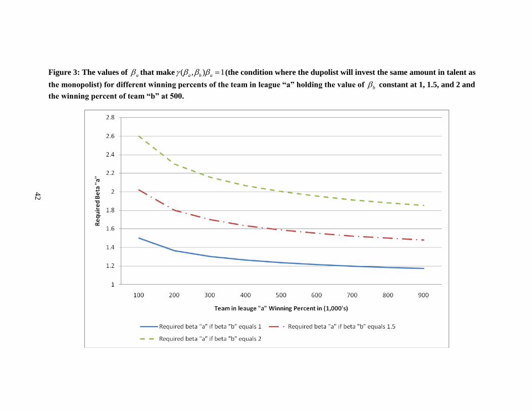
( , ) 1a b a to be true. Figure 3 graphs the required value of a for the condition
where the duopolist will invest the same amount in talent than the monopolist
( ( , ) 1a b a ) for the range of possible winning percentages of the team in league “a”,
holding constant at 1, 1,5, or 2b , and the winning percentage of the team in league
“b” at 500. The value of a decreases non-linearly with increases in b and increases
1aw .
The condition for the cross-owned firm to invest more in talent compared to the
monopolist is 11 1
1 1
aa a
a b
R
R R
1 1if a bR R .
16 Therefore, the condition for the cross-
owned firms to invest more in talent than the monopoly includes the effects of changes in
talent levels on the relative revenue of both its teams. If 1 0bR , the condition simplifies
16
The conditions are the same if 1 1a bR R but the numbers are negative.
35
to the case of duopolist. If 1 1a bR R , then the condition for the cross-owned firm to invest
more in talent is more difficult to satisfy than the condition for the duopolist.
The equations that calculate the strategic effects have
2
1 1 1
1
1 1 1 1
a a a
a
a b b a
dRR
w w w dw
embedded within them. Written with functional form is
1 1 1 1 1 1
1 1 1 1
1 1 1
1 1 1 1 1 1 1 1 11 1 13 2
1 1 1 1
( )
( ) ( )
a b a b a b
a b a b
a b a b a b a a ba a a
a b a b
w w w w w ww
w w w w
. The condition is positive if
1 1 1 1a b a if 1 1
1 1a b
a bw w
. Again, 1a must be greater than one for this to be
satisfied.
Section V: Conclusions
This paper has shown that if sports fans make consumption choices based on the
quality of all of the teams located in their markets that indirect competition and the
ownership structure alters an owner’s incentive to invest in talent. In addition, league
policies can have an effect on the quality of teams in other leagues. This has important
implications for policy makers. One reason that sports leagues are permitted to operate
with monopoly power is to preserve the product produced. However, cross-ownership is
a relationship between leagues. Therefore, cross-ownership is not intended to preserve
the product. In contrast, it is shown that cross-ownership reduces the quality of teams.
Beyond the normative issues and the utility fans gain from winning, incentive to invest in
talent has direct effects on completive balance and players’ salaries.
All analysis pertaining to league policies is important because they are at the
center of work-stoppages. The analysis of cross-league effects on league policies is

36
important because leagues are operated from a cartel of owners. As shown in this paper,
owners belonging to multiple cartels have different incentives than owners not belonging
to multiple cartels. This paper is a first attempt at understanding these incentives.
Extensions to this work are plenty. Empirical work is obvious. The effect of
cross-ownership on league expansion and relocation is important. The model in this
paper can be extended to analyze the effects of indirect competition and ownership
structure on competitive balance and players’ salaries. Further study into the pricing
effects and efficiency gains caused by cross-ownership is worthwhile. Models that
examine the effects of ownership structures in professional sports, beyond cross-
ownership, would be welcome additions to the literature.
The study of indirect substitutes might be more important in sports than other
industries because territorial rights have eliminated almost all direct competition. This
provides yet another unique opportunity for economists and sports researchers to explore,
test, and make useful recommendations. My analysis provides a theoretical framework
for future sports economics research to build upon.
37
REFERENCES
Bain, J. (1952). Price Theory. New York: Henry Holt & Company.
Cairns, J., Jennett, N., and Sloane, P.J. (1986). The Economics of Professional Team
Sports: A Survey of Theory and Evidence. Journal of Economic Studies 13(1):1-
80.
Church, J. and Ware, R. (2000). Industrial Organization: A Strategic Approach. Boston:
McGraw Hill Companies.
Daly, G. and Moore, W.J. (1981) Externalities, Property Rights, and Allocation of
Resources in Major League Baseball. Economic Inquiry 19(1):77-95.
Davenport, D.B. (1969). Collusive Competition in Major League Baseball, Its Theory
and Institutional Development. American Economist Fall:6-30.
Dixit, A. (1987) Strategic Behavior in Contests. American Economic Review 77(5):891-
898.
El-Hodiri, M. and Quirk, J. (1971). An Economic Model of a Professional Sports League.
The Journal of Political Economy 79(6):1302-1319.
Fort, R. (2006) Sports Economics. Second Edition. Upper Saddle River, NJ: Prentice
Hall.
Fort, R. and Quirk, J. (1995) Cross-Subsidization, Incentives, and Outcomes in
Professional Team Sports Leagues. Journal of Economic Literature 33(3):1265-
1299.
Hirshleifer, J. (1989). Conflict and rent-seeking success function: Ratio vs. difference
models of relative success. Journal of Public Choice 63(2):101-112.
Kesenne, S. (2000). Revenue Sharing and Competitive Balance in Professional Team
Sports. Journal of Sports Economics 1(1):56-65.
Neale, W.C. (1964). The Peculiar Economics of Professional Sports: A Contribution to
the Theory of the Firm in Sporting Competition and in Market Competition. The
Quarterly Journal of Economics 78(1):1-14.
NHL.com Staff (2009). 2009-10 salary cap set at $56.8 million. Friday, 06.26.2009 / 3:45
PM / http://www.nhl.com/ice/news.htm?id=431786.
Oliver, R.L. (1999). Whence Consumer Loyalty? The Journal of Marketing Special Issue
63:33-44.

38
Quirk, J. and El-Hodiri, M. (1974). The Economic Theory of a Professional Sports
League. In: R.G. Noll, ed., Government and the Sports Business pp. 33-80.
Rascher, D. (1997). A model of a professional sports league. International Advances in
Economic Research 3(3):327-328.
Robinson, J. (1954). The Economics of Imperfect Competition. London: MacMillan.
Schmalensee, R. (1982). Another Look at Market Power. Harvard Law Review 95:1789-
1816.
Skaperdas, S. (1996) Contest Success Functions. Economic Theory 7(2):283-290.
Szymanski, S. and Késenne, S. (2004). Competitive balance and gate revenue sharing in
team sports. Journal of Industrial Economics 52(1):165-177.
Tirole, J. (1988). The Theory of Industrial Organization. Cambridge, MA: The MIT
Press.
Vrooman, J. (1995). A General Theory of Professional Sports Leagues. Southern
Economic Journal 61(4):971-990.
Winfree, J. (2008). Owners incentives during the 2004-05 National Hockey League
lockout. Journal of Applied Economics 41(25):3275-3285.
Ziss, S. (1995). Vertical Separation and Horizontal Mergers. The Journal of Industrial
Economics 43(1):63-75.
39
TABLES AND FIGURES
Figure 1. The number of markets with at least 1 team from each league (MLB, NBA, and the NHL) and number of cross-owned firms.

40
Table 2. Cross-Ownership between teams in the NBA, MLB, and NHL
Location Years NBA Team MLB Team NHL Team
Phoenix 1998 – 2004 Phoenix Suns Arizona Diamondbacks
Atlanta 1976-2004 Atlanta Hawks Atlanta Braves
1999-2003 Atlanta Hawks Atlanta Braves Atlanta Thrashers
2003-present Atlanta Hawks Atlanta Thrashers
Washington17 1975-1999 Washington Wizards Washington Capitals
1999-2006 Washington Wizards Washington Capitals
Boston 1951-1963 Boson Celtics Boston Bruins
Chicago 1985-present Chicago Bulls Chicago White Sox
Dallas 1998-present Texas Rangers Dallas Stars
Denver 1995-1998 Denver Nuggets Colorado Avalanche
1998-2000 Denver Nuggets Colorado Avalanche
2000-present Denver Nuggets Colorado Avalanche
Detroit 1982-present Detroit Tigers Detroit Red Wings
Detroit/Tampa Bay Detroit Pistons Tampa Bay Lightning
Los Angeles 1967-1979 Los Angeles Lakers Los Angeles Kings
1979-1988 Los Angeles Lakers Los Angeles Kings
1999-present Los Angeles Lakers Los Angeles Kings
1997-2005 Los Angeles Angels of
Anaheim
Anaheim Ducks
Miami 1993-1998 Florida Marlins Florida Panthers
New York 1946-present New York Knicks New York Rangers
2000- 2004 New Jersey Nets New York Yankees New Jersey Devils
Philadelphia 1997-present Philadelphia 76ers Philadelphia Flyers
Toronto 1996-present Toronto Raptors Toronto Maple Leafs
Vancouver 1995-2001 Vancouver Grizzles Vancouver Canucks
17
Abe Pollin currently remains part owner of the NHL’s Washington Capitals.

41
Table 3: Summary of cross-ownership firm among cities with a team from each league (MLB, NBA, and the NHL)
Markets Cross-Ownership Group Leagues
New York Madison Square Garden Corp. & Yankee Global Enterprises LLC NBA/NHL & NBA/NHL/MLB
Los Angeles AEG Company and others NBA/NHL
Chicago Jerry Reinsdorf and other MLB, NBA
Toronto Maple Leafs Sports and Entertainment NHL, NBA
Detroit Olympia Entertainment NHL, MLB
Dallas Thomas Hicks NHL, MLB
Denver Kroenke Sports Enterprise NHL, NBA
Philadelphia Comcast Corp. NHL, NBA
Boston Boston Garden Co. NHL, NBA
Atlanta Time Warner/Atlanta Spirit LLC. NHL, NBA, MLB
Miami Wayne Huizenga NHL, NBA
Washington Abe Pollin NHL, NBA
Phoenix Jerry Colangelo NBA, MLB
Minneapolis NA NA
42
Figure 3: The values of a that make ( , ) 1a b a (the condition where the dupolist will invest the same amount in talent as
the monopolist) for different winning percents of the team in league “a” holding the value of b constant at 1, 1.5, and 2 and
the winning percent of team “b” at 500.

43
Appendix A: Derivations of Theoretical Equations
The condition for the duopolist to invest more in talent than the monopolist given
by equation (7) is derived by setting (5) greater than (3) as follows:
1 1 1 1 1 11 1
1 1 1 1 1 1
1 1 1 1 1 11 1
1 1 1 1 1 1
1 1 11 1
1 1 1
1 11 1
1 1
1 11 1
1 1
1 1
1
1
a a a a a aa a
a a a a a a
a a a a a aa a
a a a a a a
a a aa a
a a a
a aa a
a a
a aa a
a a
w dR w dR wR
w t dw t dw t
w dR w dR wR
w t dw t dw t
dR dRR
w dw dw
dRR
w dw
wR
w
1 1
1 1
1 1 1 11
1 1 1 1 1
1 1 , 1 1 ,
11
1
a a
a a
a a a aa
a a a a a
a a w a a r w
dR w
dw
w dR w
w dw R
R R
The strategic effect on talent is given by equation (8)
2 2
1 1 1 1 1 11
1 1 1 1 1 1 1 1
a a b a a aa
a b a b a b b a
w w dRR
t t t t w w w dw
The functions 1 1
1 1
anda b
a b
w w
t t
are both positive. Therefore the sign of (8) is
determined by the sign of the terms in the brackets. The sign of each of the four
respective terms in the brackets are: 2
1 1 11
1 1 1 1
a a aa
a b b a
dRR
w w w dw
(ambiguous)(positive)+(negative)(positive). Therefore, talent acts as strategic
compliments if
2
1 1 11
1 1 1 1
a a aa
a b b a
dRR
w w w dw
and strategic substitutes otherwise. Similarly

44
the condition for the cross-owned firm to invest more in talent than the monopolist given
by equation (12) is derived by setting (11) greater than (3) as follows:
1 1 11 1 1
1 1 1
1 1 1 1 1 1 1 11 1 1
1 1 1 1 1 1 1 1
1 1 1 11 1 1
1 1 1 1
1 1 11 1 1
1 1 1
1
(1 )
1
a b aa b a
a a a
a a a a b a a aa a b
a a a a a a a a
a b a aa b a
a a a a
a b aa b a
a a a
a
dRR R
w w dw
w dR w w dR wR R
w t dw t w t dw t
dR dRR R
w w dw dw
dRR R
w w dw
1 1 1 1
1 1 1 1 1 1
1 1 1, 1 1 ,
1 1 1
1 1 , 1 1 , 1 1 ,
1
1
a a a a
a a b a a a
b a bw a a R w
a a a
a a w b b w a a R w
w R
w R
R R R
The strategic equation in equation (8) is derived as follows:
2 2
1 1 1 1 1 11
1 1 1 1 1 1 1 1
1 1 1 1 11 1
1 1 1 1 1 1 1
2
1 1 1 1 1 11
1 1 1 1 1 1 1
1
a a b a a aa
a b a b a b b a
a a a a aa a
b a b a a a a
a b a a b aa
a b b a b b a
w w dRR
t t t t w w w dw
w dR wR
t t t w t dw t
w w w dRR
w w t t w t dw
1
1
2
1 1 1 1 11
1 1 1 1 1 1
a
a
a b a a aa
a b a b b a
w
t
w w dRR
t t w w w dw
The derivations of the other of the strategic effects are similar.
The equations for the effects of revenue sharing on other leagues are derived by
setting the two first order conditions equal to each other and using the two-team league
model equilibrium condition of 1 2
1 1
b b
b b
w w
t t
. This results in the following series of
equations resulting in equation (20).

45
1 1 1 2 1 1 1 1 2 21 1 1 1
1 1 1 2 1 2 1 1 2 2
1 1 1 1 1 11 1 1 1
1 1 1 2 1 1
1 1
1
b b b b b b b b b bb b b b
b b b b b b b b b b
b b b b b bb b b b
b b b b b b
w dR dR w w dR dR wR R
t w dw dw t t w dw dw t
w dR w dRR R
t w dw t w dw
2 2 1
2 2 1
1 1 1 1 2 2 11 1
1 1 1 2 2 2 1
1 1 11 1
1 1 1
1 1
1 1
1
1 1
and then,
1
b b b
b b b
b b b b b b bb b
b b b b b b b
b b bb b
b b b
b b
b b
dR w w
dw t t
dR w w dR w wR
dw w t t dw t t
dTR dRR
dw w dw
dTR w w
dw t
2 2 2 1
2 2 2 1
1b b b b
b b b b
dR w w
t dw t t

46
The equation for the effects of revenue sharing on cross-ownership is determined
by differentiating the first order condition,
2
1, 1
1
a b
at
, to obtain equation (23) in the
following way.
1 1 1 1 2
1
1
1, 1 1 11 1 1 1 2
1 1 1
1 1 1 2 1
1 1 1 2
1
1 1
, ( ( ), ( ))
, ( ( ), ( ))
( ( ), ( )),( ( ), ( )
,and
a a b b b
a
a
a b a aa a b b b
a a a
b b b b a
b b b b
a
a a
w w t tR
w
w dRw w t t
t t dw
w t t wR w t t
w
w w
1 1 2
1
1
2
1 1 1 1 21
1 1 1 2
11 1 1 1 2
1
1 1 1 1 2 1
1 1 2 1
( ( ), ( ))
,
and , ( ( ), ( ))
,
and
b b b
a
a
a b b b ba
a b b b
aa a b b b
a
a b b b b a
b b b a
t tR
w
w dt w dtR
w w t d t d
dRw w t t
dw
w dt w dt dR
w t d t d dw
1 1 1 2 1
1 1 1 2
1
2
1 1 1 1 1 2 1 1 1 1 21
1 1 1 2 1 1 1 2
2
1, 1 1
1
( ( ), ( )),( ( ), ( )
therefore,
b b b b a
b b b b
a
b b b b b b b b b b bb
a b b b a b b b
a b a
a a
w t t wR w t t
w
dR w dt w dt w dt w dtR
w dw t d t d w w t d t d
w
t t
2
1 1 1 1 21
1 1 1 2
1 1 1 1 2 1
1 1 1 2 1
1 1 1 1 1 2
1 1 1 2
2
1 1 11
1 1 1
a b b b ba
a b b b
a b b b b a
b b b a
b b b b b b
a b b b
b b b bb
a b b
w dt w dtR
w w t d t d
w dt w dt dR
w t d t d dw
dR w dt w dt
w dw t d t d
w dt wR
w w t d
1 2
2
2 2
1 1 1 1 2 1 1 1 1 1 11 1
1 1 2 1 1 1 1 1 1 1 1
1
1
b
b
a b b b b a a a b b ba b
a b b a b b a a b a b
a
a
dt
t d
w w dt w dt dR dRR R
t t d t d w w w dw w dw w w
w w
t
2 2
1 1 1 2 1 1 1 1 1 11 1
1 2 1 1 1 1 1 1 1 1
b b b b a b a a b ba b
b b a b a b b a a b
dt w dt dR dRR R
t d t d w w w w w dw w dw

47
The condition for proposition 7 is as follows. If 1 1 1 2
1 2
0b b b b
b b
w dt w dt
t d t d
the
equation (23) is positive (negative) if the term in the square brackets is negative
(positive). Therefore revenue sharing acts as strategic compliments if
2 2
1 1 1 1 1 11 1
1 1 1 1 1 1 1 1
a b a a b ba b
a b a b b a a b
dR dRR R
w w w w w dw w dw
and strategic substitutes
otherwise.
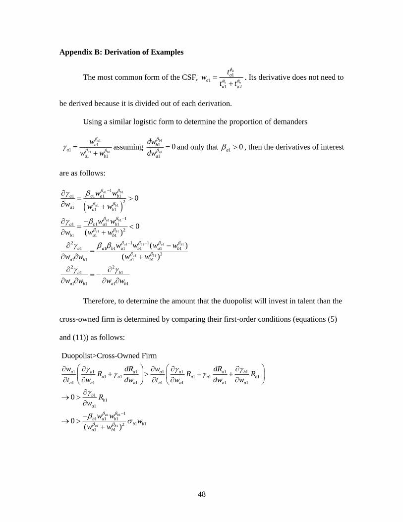
48
Appendix B: Derivation of Examples
The most common form of the CSF, 11
1 2
a
a a
aa
a a
tw
t t
. Its derivative does not need to
be derived because it is divided out of each derivation.
Using a similar logistic form to determine the proportion of demanders
1
1 1
11
1 1
a
a b
aa
a b
w
w w
assuming
1
1
1
1
0b
a
b
a
dw
dw
and only that 1 0a , then the derivatives of interest
are as follows:
1 1
1 1
1 1
1 1
1 1 1 1
1 1
1
1 1 1 1
2
11 1
1
1 1 1 1
2
1 1 1
1 12
1 1 1 1 1 1 1
3
1 1 1 1
2 2
1 1
1 1 1 1
0
0( )
( )
( )
a b
a b
a b
a b
a b a b
a b
a a a b
aa b
a b a b
b a b
a a b a b a b
a b a b
a b
a b a b
w w
w w w
w w
w w w
w w w w
w w w w
w w w w
Therefore, to determine the amount that the duopolist will invest in talent than the
cross-owned firm is determined by comparing their first-order conditions (equations (5)
and (11)) as follows:
1 1
1 1
1 1 1 1 1 1 11 1 1 1 1
1 1 1 1 1 1 1
11
1
1
1 1 11 12
1 1
Duopolist>Cross-Owned Firm
0
0( )
a b
a b
a a a a a a ba a a a b
a a a a a a a
bb
a
b a bb b
a b
w dR w dRR R R
t w dw t w dw w
Rw
w ww
w w

49
Condition where the duopolist will invest more in talent compared to the
monopolist: Equation 7
1 1 1
1 1 1 1
1 1 1
1 1 1 1
1 1
1 1
1 11 1
1 1
1
1 1 1 11 1 12
1 1 1 1
1
1 1 1 112
1 1 1 1
1
1 1 1 112
1 1
(1 ) (7)
1( )
1( )
( )
a b a
a b a b
a b a
a b a b
a b
a b
a aa a
a a
a a b aa a a
a b a b
a a b aa
a b a b
a a ba
a b
dRR
w dw
w w ww
w w w w
w w ww
w w w w
w w ww
w w
1
1 1
1 1 1 1 1
1 1 1 1 1 1
1 1 1 1
1 1
1 1
1
1 1
1
1 1 1 1 1 1 1
1
1 1 1 1 1 1 1 1
1 1 1 11 1
1 1 1
1 11
1
1
1
1 1
1
1
b
a b
a b b a b
a b a b b b
a b b b
a b
a b
a
a b
a a b a b a b
a a b a a b b b
a b b ba
a b a
a ba
a
a
a
a a
w w
w w w w w w
w w w w w w w
w w w w
w w w
w w
w

50
Condition where the cross-owned firm will invest more in talent compared to the
monopolist: Equation 12
1 1 1
1 1 1 1
1 1 11 1 1
1 1 1
1 1
1 1
1 11 1 1
1 1
1
1 1 1 11 1 12
1 1 1 1
(1 )
with the logistic specification:
( ) (1 )
( ) 1( )
a b a
a b a b
a b aa b a
a a a
a b
a a
a aa b a
a a
a a b aa b a
a b a b
dRR R
w w dw
w w
dRR R
w dw
w w wR R
w w w w
1 1 1
1 1 1 1
1 1
1
1
1 1 1 11 1 12
1 1 1 1
1 1 1 11 1 1
1
1 1 1 1
1
1 1 1 1
11 1 1 1
1 1
11 1
1 1
( )( )
( )( )
1( )
( )
if , or( )
i( )
a b b
a b a b
a b
a
a a b ba b a
a b a b
a b a aa a b
a
a a b a
a
a a b a
aa a a b
a b
aa a
a b
w w wR R
w w w w
w w wR R
w
R R R
R R R
RR R
R R
R
R R
1 1f ,a bR R
The simplification of strategic effects is as follows. All of the strategic effects
have
2
1 1 1
1
1 1 1 1
a a a
a
a b b a
dRR
w w w dw
embedded within them. Using the functional forms, this
equation is positive if1 1 1 1 1 1
1 1 1 1
1 1 1
1 1 1 1 1 1 1 1 11 1 13 2
1 1 1 1
( )0
( ) ( )
a b a b a b
a b a b
a b a b a b a a ba a a
a b a b
w w w w w ww
w w w w
, which
simplifies to 1 1
1 1
1 11
1 1
a b
a b
a ba
a b
w w
w w
and then 1 1
1 1 1 1 11,if a b
a b a a bw w .

51
Appendix C: Details of the progression of cross-ownership
As of 1970, five markets had a team from each of the three leagues: New York,
Los Angeles, San Francisco, Boston, and Chicago. Of these five markets, three of them
included cross-ownership structures: New York, Los Angeles, and Boston – and San
Francisco only had teams from different leagues until 1973. Madison Square Garden
Corporation has owned both the New York Rangers of the NHL and the New York
Knicks of the NBA since 1946. Jack Kent Cooke first owned both the NHL’s Los
Angeles Kings and the NBA’s Los Angeles Lakers in 1967 and they remain part of the
same ownership group today, even though they have been sold four times. In Boston,
Walter Brown owned both an NHL team and NBA team for 12 years between 1951 and
1963. In 1972 Chicago’s Arthur Wirtz owned both an NBA and NHL team until he died
in 1983. Jerry Reinsdorf continued the cross-ownership trend in Chicago by
simultaneously owning both a MLB and NBA team from 1985 through to the present.
At the time of the NHL first attempt in Atlanta, 1972, the market already
consisted of MLB’s Braves and the NBA’s Hawks. In 1976, Ted Turner purchased the
Braves and the Hawks. Atlanta relocated to Calgary in 1979. The city of Atlanta ended
up becoming a three-team city again when the NHL expanded back to Atlanta in the form
of the Thrashers in 1999. However, the Thrashers were part of Time Warner that owned
each team from all three leagues18
. The NHL and NBA were sharing the market in
Washington for only three years before Capital’s owner Abe Pollin purchased the
Wizards to run the Capitals and Wizards as a single firm. Pollin continued to own both
teams until 1999 when he divested the NHL’s Capitals to owner Ted Leonis. Pollin
18
In 2003 Time Warner divested of its professional sports teams. The Thrashers and Hawks became
owned by the Atlanta Spirit and the Braves by Liberty Media Group.

52
remains as a minority shareholder. In 1995, Tom Hicks purchased the Dallas Stars and
three years later purchased the Texas Rangers. Currently, Hicks owns both the Stars and
Rangers. Similar to Atlanta, after a failed attempt, the NHL was able to be successful in
Denver as part of a cross-owned firm, Comcast Corporation, which owns both an NBA
and NHL team. Mike Illich has owned both the NHL’s Red Wings and MLB’s Tigers
franchises in Detroit since 1982 and because the NBA’s Pistons play their games out of
the city center where both the Red Wings and Tigers play, his firm owns the entire
professional sports market in downtown Detroit. The NBA was the first to move into the
Miami market, expanding to include the Miami Heat in 1998. Major League Baseball
and the NHL entered the Miami market in 1999 together under owner Wayne Huizenga.
Philadelphia was represented with individual ownership of each of the three professional
leagues prior to 1970. In 1997, Comcast-Spectator that owned the NHL’s Flyers’
purchased the NBA’s 76’ers. In 1998, MLB awarded the NBA’s Phoenix Suns owner,
Jerry Colangelo, an expansion team. Toronto Maple Leafs formed Maple Leafs Sports
and Entertainment and purchased the Toronto Raptors after they joined the city in 1998,
three years after their expansion into the city.

53
CHAPTER 3: A COMPARISON OF TELEVISION AND GATE DEMAND IN
THE NATIONAL BASKETBALL ASSOCIATION
Abstract
I estimate the demand for gate attendance and television audiences in the NBA
and find that the fans who attend games live are inherently different from fans who watch
games on television. Fans who watch the games on television are more sensitive to
winning, and do not substitute for other professional sports leagues, compared to fans
who attend the games. The effects of winning on demand for television compared to gate
attendance can have consequences for competitive balance.

54
INTRODUCTION
Although media is an important and growing revenue source for sports teams,
little is known about the factors of demand for games on television. For the 2007-08
season, the National Basketball Association (NBA) received $4.6 billion from league-
wide contracts from ABC/ESPN and AOL/Time Warner, and this does not include local
television rights. Media revenue typically accounts for over one-third of total revenue for
teams in the NBA, and it is sometimes greater than stadium revenue. However, a vast
majority of the literature that estimates demand for sports teams, estimates attendance.
This is somewhat understandable since attendance data is typically easier to obtain.
Nonetheless, given the growing importance of media revenue, more needs to be known
about fans who watch games on television. The goal of this study is to estimate
television demand for the NBA and compare and contrast this with demand for
attendance.
I analyzed annual local media television ratings to see how fans who watch NBA
games on television are inherently different from fans who watch the games in person. It
has been well documented that factors such as team quality, income, population, and
substitutes will affect sports attendance, but little is known about these effects on
television audiences for sports teams. It may be the case that fans who watch the NBA
on television are generally a different group from fans who typically go to the game. It
may also be the case that certain variables cause a substitution between television and
attendance. Regardless, teams and researchers should have some understanding of the
different types of demand. For example, it may be the case that NBA attendance is a

55
normal good, but the NBA television audiences are an inferior good. Therefore, the
effect of incomes on a team’s revenue may be ambiguous, which may affect the
feasibility of potential markets.
Much of the literature on the demand for sports television has focused on the
substitution between watching a game on television and watching a game live for
European football fans (Baimbridge et al. (1996), Allan (2004), Forrest et al. (2004),
Buraimo et al. (2006), Buraimo (2008), Allen and Roy (2008)), Rugby fans (Baimbridge
et al. (1995), Carmichael et al. (1999)), college football fans (Kaempfer and Pacey
(1986), Fizel and Bennett (1989)) and National Football League fans (Siegfried and
Hinshaw (1979), Zuber and Gandar (1988), Putsis and Sen (2000)). Other factors for
television, such as uncertainty of outcome (Forrest et al., 2005), have been found to be
significant factors affecting the demand for television audiences.
Much of the analysis of the NBA is focused on salary discrimination (Becker
(1971), Kahn (1991) Wallace (1998), Jenkins (1996), Hamilton (1997), Kanazawa
(2001), Bodvarsson (1999 and 2001)), and productivity (Kock (1988), McCormick
(2001), Berri (2006)), while some analysis is concentrated on the demand for particular
players and their externalities (Hausman and Leonard (1997), Berri (2004)). Another line
of research draws attention to the impact and motivation of rule changes in the NBA.
Taylor (2002) examines how the introduction of the NBA draft lottery reduced the
incentive of teams that were eliminated from the playoffs to lose games, and Caudill
(1998) argues that the NBA changed its playoff format to increase revenue rather than to
reduce travel time for teams. Some studies have focused on gate demand. Leadly and
Zygmont (2005) examine new-facility effects on demand in a number of professional

56
sports including the NBA. Centering on race, Burdekin and Hossfeld (2005) and
Burdekin and Idson (1991) estimate gate demand. They find that customer preferences
toward race influence gate revenues. Similarly, using Nielsen ratings for local television
NBA games, Kanazawa and Funk (2005) find that television viewership increases when
there is a greater participation by players who are white.
Besides being a critical part of the team’s revenue stream, the sensitivity of
television fans to winning can also alter an owner’s incentive to invest in winning.
Therefore win percent is a key variable to understand. Television fans’ preferences to
winning alone can either improve or reduce competitive balance in leagues.
Data and Empirical Estimation
In this article, demands for attendance and television are estimated for 6 years
from the 1999-00 to the 2004-05 seasons. Nielsen local cable ratings are used to derive
television attendance for US based teams. Nielsen ratings are a statistical estimate of the
percentage of people watching a particular television program within the designated
marketing area (DMA).
Since the Nielsen ratings data represents the average viewership in the area per
game, I construct a metric that approximates per capita season television audience. Using
this data I derive the size of the per capita annual television audience as:
Per Capita TV Attendance Neilson Ratings Number of Games (1)

57
Given the nature of the professional sports television market in the United States, I make
the assumption that all games are televised on local cable networks, setting the number of
games televised to 82 for all teams.
Between the 1999-00 and 2004-05 seasons there were two team relocations: the
Charlotte Hornets relocated to New Orleans, and the Vancouver Grizzlies relocated to
Memphis for the start of the 2002-03 season. Nielsen ratings were unavailable for nine
years dispersed throughout that data and were therefore not included. Also, Nielsen
reported ratings for two different television stations in the case of Atlanta and Chicago
for 5 and 4 of the years respectively, which are averaged. The attendance data were
adjusted to have the identical sample as television, resulting in 158 observations for both
television and gate attendance.
I use two empirical models to estimate demand. Each is a linear regression
model, the first with time effects, and the second with both time and team effects. I have
estimations with and without team fixed effects so I can estimate the effects of variables
that are team specific, but the empirical data do not vary over time. Since our sample
covers a relatively short period of time (six years) and income data does not vary
substantially, I include a model with only time effects to compare the effects and income
between attendance and television. The empirical specifications are as follows:
tiv
k
j
tjtiti
tititititiv
YearOtherSUBSNBASUBS
PayIncomeWinPriceAtt
,,
1
6,6,5
,4,3,2,1,, lnln%lnln
(2)
n
m
tivimk
k
j
tjtiti
tititititiv
TeamYearOtherSUBSNBASUBS
PayIncomeWinPriceAtt
1
,,6
1
6,6,5
,4,3,2,1,, lnln%lnln
(3)

58
where , ,v i tAtt is the yearly per capita attendance for viewing method v (gate and
television), for team i in year t , Price is the weighted average ticket price, %Win is the
team’s winning percentage, Income is the city’s average income according to the Census
Bureau in 2003, NBASUBS and OtherSUBS are the number of NBA teams and other
professional sports teams within the SMSA respectively, Pay is the team’s payroll, and
Year19
and Team are fixed effects20
. Per capita gate attendance is normalized by the
standard metropolitan statistical area (SMSA). Given our derivation of TV attendance,
deriving per capita estimates allows us to avoid having population in the dependant and
independent variables, reducing the likely possibility of contaminating the structure of the
errors. For the remainder of the paper I will refer to both gate and TV attendance,
assuming it is per capita. The summary statistics are given in table 1.
Empirical Results
The presence of heteroskedasticity and autocorrelation were tested with regard to
ordinary least squares. Heteroskedasticity was tested using a Breusch-Pagan/Cook-
Weisberg test and was not found to be significant (the hypothesis of constant variance
could not be rejected) in the estimation for TV attendance and was found to be significant
in the estimation for gate attendance. Autocorrelation was found to be significant in all
equations using a Wooldridge test (the hypothesis of no first order-autocorrelation was
rejected). Based on these tests, heteroskedasticity and autocorrelation were corrected for
using generalized least squares (GLS).
19
Fixed effects for each year is included in the estimation, therefore a constant term would make the X
matrix completely dependent. 20
This data can be found at rodneyfort.com. All of the data in the sample were originally from USA
Today.

59
Table 2 presents the results of the demand estimations. The results show that
consumers who attend the games live are an inherently different group of consumers
from fans who watch the games on television. Attending a live game is an all-inclusive
event that consumers most likely attend with family and friends and might include other
activities, such as dinner. Fans who attend the games live are less sensitive to income,
sensitive to the quality of the team (win percent), and sensitive to sports substitutes inside
and outside of the NBA. In comparison, fans watching the games on television are more
sensitive to income effects, and demand their NBA team to win.
Focusing on the model without fixed effects, I estimated the relationship of
income with both television and gate attendance. Income has little-to-no effect on gate
attendance, and because consumers generally do not specifically pay to watch local
television games, it might be considered a type of quasi-inferior good to television
attendance with a negative and significant income elasticity of 1.855. I noted that a
longer time span of data might provide better estimates of the income variables since it
would be more informative to add these variables to a model with team fixed effects.
For the rest of the variables, I primarily focused on the fixed effects models while
making an holistic interpretation from all of the results. Although not significant, the
coefficients of the price variables do represent price elasticities. As with most of the
sports economics literature, I found that teams price tickets in the inelastic portion of
demand, with an estimated elasticity of approximately 0.09. This could be due to
behavior factors such as the development of habit formation or additional revenue from
concessions or stadium advertising. Consistent with intuition and the income effect

60
previously discussed, higher ticket prices result in greater television demand, evidenced
by the positive price elasticity.
In support of other recent findings, both within league and across leagues act as
substitute products with the NBA – although more so with gate attendance than with
television. I modeled substitution between sports teams as discrete shifts, so the
coefficients in the regressions shift demand down. The number of other NBA teams in
the market had a negative and significant impact on both television audience and
attendance. These results continue to show significant impact of territorial rights that
limit the direct competition. With territorial rights firmly entrenched in the market and
no reason to think that change is near, research on the effects of indirect substitutes, such
as other sports leagues, is an important economic finding. Teams acting as indirect
substitutes for other leagues have significant effects on both television and attendance.
The substitution effect on attendance is consistent with prior evidence that consumers
trade off between professional sports. The substitution effect on television audiences has
been previously unexplored and is weaker than gate attendance. This weakness could be
because, in the absence of prices, television audiences choose to either watch their NBA
team or not, depending on whether they are winning. That is, when consumers do not
have to pay for sports, they might be considered fickle.
Payroll effects essentially have no effect on attendance and have an ambiguous
effect on television audiences. Both fans who view the game live and fans who view on
television have preferences toward the actual quality of the team (win percent) rather than
individual talent within the team (payroll).
61
Perhaps one of the most interesting implications of the results is the difference in
consumers’ preferences towards winning. Realizing the revenue generated from
television is substantial, television audiences’ sensitivity toward winning enters into the
owners’ decision problem and, all else constant, can influence the league’s competitive
balance. The investment in talent made by team owners depends on the contribution of
winning to revenue. With teams in geographical locations with varying revenue
potentials, the possibility exists for television audiences’ sensitivity for winning to have
an effect on competitive balance within the league. Although I am unable to determine
the complete marginal revenue of winning from television, the results that I derived do
uncover part of the equation: the effects of winning on television demand. From the
results, a 1 point increase in a team’s win percent increases television attendance by 1.5%
and gate attendance by 0.3%.
The difference in sensitivity to winning may also have implications for the
effectiveness of revenue sharing programs. Revenue sharing essentially reduces the
incentive for owners with higher marginal revenue of winning to invest in talent.
Recognizing that winning is more important to television audiences than attendance,
these findings have policy implications regarding the effectiveness of the instruments
used to improve competitive balance.

62
CONCLUSION
Because media revenue is such a substantial amount of the revenue that owners
generate through team operations and little is currently known about the factors that
affect demand, I estimated and compared the results of television and gate demands.
While there is undoubtedly much overlap between fans who attend the games and
television fans, it appears that fans watching television are an entirely different group
than fans who attend games. Fans who watch the games on television are more price
sensitive, demand more winning, and do not substitute for other professional sports,
compared to fans who attend games. These findings are also an important component of
competitive balance.

63
REFERENCES
Allan, G. and Roy, G. (2008). Does Television Crowd Out Spectators? New Evidence
from the Scottish Premier League. Journal of Sports Economics (forthcoming).
Allan, S. (2004). Satellite television and football attendance: The not so super effect.
Applied Economics Letters 11:123-125.
Baimbridge, M., Cameron, S., and Dawson, P. (1995). Satellite broadcasting and match
attendance: The case of rugby league. Applied Economics Letters 2(10):343-346.
Baimbridge, M., Cameron, S., and Dawson, P. (1996). Satellite television and the
demand for football: A whole new ball game. Scottish Journal of Political Economy
43(3):317-333.
Becker, G. (1971). The Economics of Discrimination. Second edition. Chicago:
University of Chicago Press.
Berri, D.J., Schmidt, M.B., and Brook, S.L. (2004). Stars at the Gate: The Impact of Star
Power in NBA Gate Revenues. Journal of Sports Economics 5(Feb):33-50.
Berri, D.J., and Schmidt, M.B. (2006). On the road with the National Basketball
Association’s Superstar Externality. Journal of Sports Economics 7(4 Nov):347-358.
Burdekin, R.C.K., Hossfeld, R.T., and Smith, J.K. (2005). Are NBA Fans Becoming
Indifferent to Race? Evidence from the 1990s. Journal of Sports Economics 6(2
May):144-159.
Burdekin, R.C.K. and Idson, T.L. (1991). Customer Preferences, Attendance, and the
Racial Structure of Professional Basketball Teams. Applied Economics
23(January):179-186.
Bodvarsson, O.B. and Brastow, R.T. (1999). A Test of Employer Discrimination in the
NBA. Contemporary Economic Policy 17:243-55.
Bodvarsson, O.B. and Partridge, M.D. ( 2001). A Supply and Demand Model of Co-
Worker, Employer and Customer Discrimination. Labour Economics 8:389-416.
Buraimo, B., Forrest, D., and Simmons, R. (2006). Robust estimates of the impact of
broadcasting on match attendance in football (Working paper no. 2006/004).
Lancaster University Management School, England.
Buraimo, B. (2008.) Stadium Attendance and Television Audience Demand in English
League Football. Managerial and Decision Economics 29:513-523.

64
Carmichael, F., Millington, J., and Simmons, R. (1999). Elasticity of demand for rugby
league attendance and the impact of BskyB. Applied Economics Letters 6:797-800.
Caudill, S.B. and Mixon, F.G., Jr. (1998). Television Revenue and the Structure of
Athletic Contests: The Case of the National Basketball Association. Eastern
Economic Journal 24(Winter):43-50.
Fizel J.L. and Bennett, R.W. (1989). The impact of college football telecast on college
football attendance. Social Science Quarterly 70:980-988.
Forrest, D., Simmons, R., and Buraimo, B. (2005). Outcome uncertainty and the couch
potato audience. Scottish Journal of Political Economy 52(4):641-661.
Forrest, D., Simmons, R., and Szymanski, S. (2004). Broadcasting, attendance and the
inefficiency of cartels. Review of Industrial Organisation 24:243-264.
Hamilton, G.H . (1997). Racial Discrimination and Professional Basketball Salaries in the
1990s. Applied Economics 26:287-96.
Hausman, J.A. and Leonard, G.K. (1997). Superstars in the national basketball
association: economic value and policy. Journal of Labor Economics 15(4):586-624.
Jenkins, J.A. (1996). A reexamination of Salary Discrimination in Professional
Basketball. Social Science Quarterly 77(3):594-608.
Kaempfer, W.H. and Pacey, P.L. (1986). Televising college football: the
complementarity of attendance and viewing. Social Science Quarterly 67:176-185.
Kahn, L. (1991). Discrimination in Professional Sports: A Survey of the Literature.
Industrial and Labor Relations Review 44(3/Apr):395-420.
Kanazawa, M.T. and Funk, J.P. (2001). Racial Discrimination in Professional
Basketball: Evidence from Nielsen Ratings. Economic Inquiry 39(October):599-
608.
Kock, J.V. and Vander Hill, C.W. (1988). Is There Discrimination in the Black Man’s
Game? Social Science Quarterly 69(1):83-94.
Leadly, J.C. and Zygmont, Z.X. (2005). When Is the Honeymoon Over? National
Basketball Association Attendance 1971-2000. Journal of Sports Economics 6(2/
May):203-221.
McCormick, R.E. and R.D. Tollison. (2001). Why Do Black Basketball Players Work for
Less Money? Journal of Economic Behavior and Organization 44(2):201-19.
65
Putsis, W.P. and Sen, S.K. (2000). Should NFL blackouts be banned? Applied Economics
32:1495-1507.
Siegfried, J.J. and Hinshaw, C.C. (1979). The effect of lifting television blackouts on
professional football no-shows. Journal of Economics and Business 31:1-13.
Taylor, B.A. and Trogdon, J.B. (2002). Losing to Win: Tournament Incentives and the
Draft in the National Basketball Association. Journal of Labor Economics 20(1):23-
41.
Wallace, M. (1998). Labor Market Structure and Salary Discrimination among
Professional Basketball Players. Work and Occupations 15(3):294-312.
Zuber, R.D. and Gandar, J.M. (1988). Lifting the TV blackout on no-shows at football
games. Atlantic Economic Journal 16:63-73.

66
TABLES
Table 1. Summary Statistics
Variable Min Max Mean SD
ln(Gate Attendance) -2.834 -0.496 -1.486 0.608
ln(TV Attendance) -1.115 1.881 0.514 0.663
Gate Attendance 0.059 0.609 0.267 0.141
TV Attendance 0.328 6.560 2.041 1.258
ln(Income) 10.217 10.878 10.504 0.141
ln(Payroll) 17.050 18.520 17.832 0.227
Win Percent 0.159 0.817 0.506 0.151
No. NBA Substitutes 0.000 1.000 0.076 0.266
No. Other Substitutes 0.000 6.000 2.278 1.604

67
Table 2. Demand Estimation for Television and Gate Attendance ln(television attendance per capita) ln(gate attendance per capita)
With Time and Team
Effects With Time Effects
With Time and Team
Effects With Time Effects
Coefficient
Estimates t-statistics
Coefficient
Estimates t-statistics
Coefficient
Estimates t-statistics
Coefficient
Estimates t-statistics
ln(price) 0.142 0.55 0.250 1.06 -0.088 -1.27 -0.115 -0.95
ln(income) -1.855*** -2.63 -0.558 -1.08
Win Percent 1.521*** 5.75 1.354*** 5.45 0.332*** 4.97 0.263*** 3.76
ln(payroll) -0.282 -1.24 0.071 0.32 0.041 0.72 0.02 0.33
No. NBA Subs -1.454*** -5.59 -0.593 -1.54 -0.968*** -16.5 -0.912*** -4.57
No. Other Subs -0.100*** -2.98 0.001 0.02 -0.261*** -40.09 -0.225*** -6.72
1999-00 4.725 1.15 17.224*** 2.21 -1.411 -1.39 4.952 0.93
2000-01 4.74 1.15 17.142*** 2.20 -1.421 -1.39 4.924 0.93
2001-02 4.718 1.14 17.115*** 2.20 -1.433 -1.41 4.905 0.92
2002-03 4.747 1.15 17.048*** 2.20 -1.442 -1.41 4.871 0.92
2003-04 4.907 1.19 17.200*** 2.22 -1.44 -1.41 4.861 0.92
2004-05 4.812 1.16 17.070*** 2.21 -1.401 -1.37 4.882 0.92
ATLANTA -1.116*** -4.70 -0.283*** -4.82
BOSTON -0.503*** -4.22 -0.544*** -15.21
CHARLOTTE -1.068*** -4.57 0.162 1.11
CHICAGO -0.084 -0.39 -0.293*** -4.74
CLEVELAND -0.287 -0.83 0.163* 1.95
DALLAS -0.352 -1.84 0.074 1.58
DENVER -0.319 -1.39 0.493*** 9.6
DETROIT 0.001 0.00 -0.139 -1.94
GOLDEN STATE -0.281 -1.02 0.828*** 10.88
HOUSTON -0.19 -1.36 -0.57*** -8.76
INDIANA 0.181 1.37 0.268*** 7.53
LOS ANGELES 1.644*** 6.15 0.366*** 6.12
MEMPHIS -0.391*** -2.3 0.277*** 6.49
MIAMI -0.677*** -4.86 0.453*** 12.5
MILWAUKEE -0.308 -1.48 0.298*** 6.29
MINNESOTA -0.351 -1.50 0.144*** 2.95
NEW YORK -1.521 -7.27 -0.063 -1.63
NEW ORLEANS -0.19 -0.57 0.347*** 6.15
ORLANDO -0.095 -0.42 -0.134*** -4.61
PHILADELPHIA -0.009 -0.06 -0.242 -5.2
PHOENIX -0.164 -0.93 0.111*** 2.99
PORTLAND -0.319 -1.03 -0.079 -1.63
SACRAMENTO - - - -
SAN ANTONIO 0.283*** 2.71 0.13*** 2.25
SEATTLE -0.045 -0.23 0.035 1.22
SALT LAKE CITY -0.105 -0.44 0.003 0.39
WASHINGTON -0.31 -1.21 -0.248*** -3.74

68
CHAPTER 4: CONTEST SUCCESS FUNCTIONS AND MARGINAL PRODUCT
OF TALENT
Abstract
Although tournaments, conflicts, rent-seeking, and sporting events have been modeled
with contest success functions, little empirical support exists for choosing the appropriate
form. The difference and ratio forms have been identified by researchers as popular
choices to develop theoretical properties and model professional sports leagues. In this
article, a multi-stage regression is used to estimate the parameters of difference and ratio
forms of the contest success functions. The forms are then compared for best fit using
various criteria. The evidence suggests that the ratio form is closest to the true
specification. Furthermore, parametric estimates of the ratio form are proved to support
the simplifying assumption made by most sports economists that the mass or talent
parameter is equal to one. The contest success function is further used to determine the
contribution to winning of the candidate players for the 2010 Canadian Men’s Olympic
Hockey Team.
69
INTRODUCTION
Empirical economic modeling involves understanding the underlying production
process and specifying the appropriate functional forms. Different from traditional
production theory, the economics of contests are complicated by the fact that output
depends on the relationship between the firms in the industry who are the contestants. A
contest is a game in which players increase the probability of winning by exerting effort
with the objective of obtaining a prize (Skaperdas, 1996). A contest success function
(CSF) describes the production process and the interdependent relationship among the
effort of participants and winning. Although the theory of contests and CSFs has
progressed forward, substantial empirical analysis is missing. Skaperdas (1996) points
out that empirical support for choosing the particular form of the CSF would be a
welcome endeavor. This article empirically estimates two forms of the CSF and
compares the fit of each model. The analysis is extended to calculate the contribution to
winning of the 2010 Canadian Men’s Olympic Hockey Team candidate players.
The literature on contests can be divided into three groups: topics, production,
and empirical estimation. The economic perspective of contests has been used to
describe many different topics including R&D rivalries (Loury (1979), Dasgupta and
Stiglitz (1980), Lee and Wilde (1980)), rent-seeking conflict (Tullock (1980), Nitzan
(1991), Baye et al. (1993)), political campaigns (Skaperdas and Gorfman (1995)),
incentive design (Lazear and Rosen (1981), Green and Stokely (1983), Holmstrom
(1982), Nalebuff and Stiglitz (1983), and Rosen (1986)) and sporting events (Fort and
Winfree (2009), Rascher (1987), Szymanski (2003, 2004), Szymanski and Kesenne

70
(2004), Kesenne (2005, 2006)). Economists have also studied the production of contests
through strategic commitment (Dixit, 1987), axioms (Skaperdas, 1996), Clark and Riis
(1996), Blavatskyy (2008)), incentives (Epstein and Nitzan (2006)), and forms (Jia
(2008), Hirshleifer (1989), Cornes and Hartley (2003), Rai and Sarin (2007), Corchon
and Dahm (2007)). To the best of the author’s knowledge, there is only one paper that
empirically estimates CSFs. Hwang (2007) created a Bayesian statistic to compare
different logit forms of the CSF using war data and suggests that the ratio form performs
best in predicting the probability of winning war battles.
The functional form used to model the underlying process of a production process
can change the analytical properties. Currently, there is no consensus about the most
appropriate choice of functional form to empirically estimate contest models. The
purpose of this article is to compare the properties of two popular functional forms. The
data used to estimate the CSF is from the National Hockey League (NHL). Sporting
events are a good environment to empirically estimate and test the properties of CSF for
three reasons. First, sporting contests produce wins and the structure of each contest is
identical and repeated; second, contest-level data are available; and third, winning is a
determinant of the owner’s profit maximizing objective function21
. Further, professional
sports are a billion dollar industry and proper modeling of sports contests supported with
theory will also be of interest to fans, investors, and odds makers. Therefore, the fully
parameterized CSF places value on the specific actions that contribute to winning. From
a management perspective, placing value on the factors that contribute to winning can be
used to determine players’ contribution to winning, marginal revenue products, and game
strategy decisions. The results are used to calculate the contribution to winning of the
21
This assumes identical rules for each contest.

71
players who were being considered for Canada’s 2010 Men’s Olympic Hockey Team.
The approach differs from prior methods previously used in the sports economics
literature by imposing a structural model and using contest level data compared to prior
methods that do not use and model and season level data.
Evidence suggests that the ratio form of the logit model is a better fit than the
difference form of the logit model. The remainder of the paper is as follows: The models
are developed and discussed in section 2, the empirical estimation is in section 3, the CSF
diagnostics are presented in section 4, the contribution to winning calculation is presented
in section 5, and the concluding comments are offered in section 6.
The Model
Consider the owners’ profit maximizing function as follows,
, , , , , ,,i g i g i g i g j g i gR w t t C t (1)
To ensure positive but decreasing marginal effects of investment in talent on revenue, I
assumed the usual conditions ,
,
0i g
i g
R
t
,
2
,
, ,
0i g
i g j g
R
t t
. The first order condition is given
by,
, , , ,
, , , ,
( )0
i g i g i g i g
i g i g i g i g
R w C t
t w t t
(2)
Where ,i g represents team 'i s profit in game g , R is revenue, w is the probability of a
win, t is talent, and C is the cost function. Team 'i s talent performs actions it
that increase (or decrease) the probability of winning the game. Therefore, the
probability that team i wins the game is ( , )i i jw t t where iw is team 'i s CSF. The CSF for

72
team i is a function of the talent of both teams. From the perspective of team i , the
following usual conditions are assumed, 0, 0, 0, 0i ii j jjw w w w .
Different forms of CSFs are used in various areas of the literature. One of the
most commonly used forms is the logistic model for its axiomatic properties (see
Skaperdas (1996), Arbatskaya and Mialon (2008), Clark and Riis (1998)). Sports
economics have focused almost entirely on the ratio form of logit model to describe the
effect of talent on winning with little reasoning, other than noting the probability of
winning as a function of relative units of talent (see for example Fort and Winfree (2009),
Szymanksi (2003)). Further, most sports economists simplify the ratio form by assuming
that the mass (or talent) parameter is equal to one without any empirical support. Outside
of sports economics, the probit model has been discussed as a viable option. Others have
created specific CSFs to describe different situations or to expand on the growing contest
literature (see Cochron and Dahm (2008) a survey of the literature).
The conditional logistic model of discrete choice developed by McFadden (1973)
has been used in many streams of the economic literature to analyze the factors
influencing probable results. Reasons for using the logit model include its foundation in
economic theory, ease of econometric estimation, and empirical model fit (Guadagni and
Little, 1983). Hirshleifer (1989) points out that ratio form of the logit model has
impractical implications in that any investment of zero results in a probability of zero, as
long as the opponent invests a small amount of effort. Since in sports the outcome of
each game is determined by differences in scoring, the difference form of the logit is a
reasonable approach to consider. However, the difference form does not permit for an
interior pure strategy Nash equilibrium (Hirshleifer, 1989).

73
The difference and ratio forms of the logit specification representing the
probability of a team 1i win in game g are,
Difference: ,
, , ,
, , , ,
exp{ } 1( , )
exp{ } exp{ } 1 exp{ ( )}
i g
i g Diff i g j g
i g j g i g j g
tw G t t
t t t t
(3)
Ratio: ,
, , ,
, 2, , ,
1( , )
1 exp{ (ln ln )}
i g
i g Ratio i g j g
i g j g i g j g
tw G t t
t t t t
(4)
where and are the mass-parameters affecting the shape of player 'i s CSF.
, ,1j g i gw w .
There are 2 primary differences between the difference and ratio form of the CSF:
(1) the underlying assumption imposed on the data, and (2) the shapes of the CSF. The
difference form does not consider the absolute value of the number while the ratio form
does. For example, in the case of hockey, the difference between 3 and 4 shots is 1 and
the ratio is 0.75, while the difference between 5 and 6 shots remains 1 while the ratio
changes to 0.83. In this case, the difference and ratio forms yield different results.
Similar to any model, the results are constrained by the underlying assumptions of the
functional form imposed. The difference form of the CSF has increasing returns to the
point where 0.5 and diminishing returns thereafter. The ratio form has this same
characteristic as long as 1 . However if 1 , the ratio form has diminishing returns
to effort throughout (Hirshleifer, 1989), although in both cases the greater the mass-
parameter the more the input contributes to winning. Since the theory does not suggest
the best choice of the CSF, I estimated and compared the results of both the difference
and ratio forms of the logit model.

74
Empirical Estimation
Many of the statistics regularly used to measure productivity are weak measures
of the underlying production process. In hockey, the number of shots on goal is a
common statistic used to measure the amount of offensive scoring chances generated.
However, every shot on goal is different, creating different levels of quality of scoring
chances. For example, a wrist shot taken from 20 feet most likely has a different
probability of resulting in a goal than a backhand taken from 40 feet. Using the same
logic, players’ shooting percentages and goaltenders’ save percentages used to measure a
player’s ability to score and a goaltender’s ability to make a save are inaccurate.
Play-by-play game data were collected for NHL games from the 2008-09 season
from nhl.com. The data contains detailed shot information as well as whether the shot
resulted in a goal. The shot information includes the following shot characteristics: shot-
type, length, advantage type, and time of shot. The player taking the shot and the
goaltender attempting to stop the shot are also included in the data. With this data, a
multi-stage recursive system is used to create more accurate measures representing the
underlying production process and estimating the parameters of the CSFs. The first
stage calculates the predicted probability that a shot will result in a goal, given certain
shot characteristics. The second stage uses the predicted probability from the first stage
as an instrument for shot quality, and then re-predicts the probability that a shot results in
a goal, given the shot quality, as well as player and goaltender characteristics. The third
stage uses the predicted values from the second stage to estimate the parameters of the
CSFs.

75
The following takes place in stage 1. Shots are differentiated by predicting the
probability that each shot taken will result in a goal given certain shot characteristics.
The empirical estimation for the probability that a shot resulting in a goal given certain
shot characteristics is,
s s sPr(Isgoal = 1)= F(shot characteristics , error ) (5)
( )F is the logistic distribution function, sisgoal is an indicator variable equaling 1 if shot
s resulted in a goal and 0 otherwise. The shot characteristics are shot-type (deflected,
tip-ins, wrap-arounds, wrist, slap, snap, and backhand), shot length (distance in feet from
the goal). Shot-types are further differentiated by defining rebounds as shots taken within
5 seconds of the previous shot. The predicted probability is a measure of shot quality.
Then, using the predicted probabilities from stage 1 as a measure of shot quality,
stage 2 predicts the probability that a shot results in a goal by incorporating players’
ability to score and goaltenders’ ability to make saves into the model. Whether from
differences in shot strength, accuracy, superior positioning, and/or other (sometimes
unobservable) characteristics, players have differing abilities to score goals. Similarly,
goaltenders have differing abilities to stop shots from becoming goals. The empirical
estimation for the probability that a shot results in a goal is further specified as,
1 , (6)s s s stgs Pr(Isgoal = 1)= F(isgoalstage player char, goaltender char, error )
where 1isgoalstage is the predicted probability from stage 1. The variable player char ,
stands for player characteristics, indicator variables grouping players on a projected goal
per season basis (e.g. 0-4 goal scorer, 5-9 goal scorer) are used as a proxy for a player’s

76
ability to score22
. The variable goaltender char , represents goaltender characteristics, and
is an indicator variable identifying the specific goaltender attempting to stop the shot.
The estimated probability from (6) is different from (5) in that it accounts for players’
and goaltenders’ contributions to shots becoming goals and only differentiates shots by
level of quality, not by their individual shot characteristics.
Empirical Results from Stage 1 and 2
In addition to the summary statistics in table 1, figures 1a to 1g show the
percentage of shots resulting in goals by each length group (5 feet) for each shot type, for
both traditional shots and rebounds. Not evident in the graphs is the relative infrequency
of rebound shots for deflected, tip-ins, and wrap-around shots. Noticeable from the
figures, the functional relationship between the probability that a shot results in a goal
and shot length is not necessarily linear or significant for all shot types. Therefore, the
empirical model was specified by observation and testing for significance of both the
linear and inverse length relationship as well as slope and shift effects of rebounds.
Empty net goals, penalty shots, shots taken from outside the offensive zone, and 64
erroneous data entries were eliminated23
. Therefore, the sample consists of 67,441 shots
that resulted in 7,024 goals.
The logistic regression results from (5) are presented in table 2. Deflections are
modeled with an intercept and inverse in length slope effect, wrap-arounds with an
intercept effect, tip-ins with an intercept and linear in length slope effect, and wrist, slap,
22
goalsProjected goals per season = ×82
games played
23 Removing shots taken from outside the offensive zone assumes that these shots were not legitimate
attempts at scoring. The offensive zone is 60 feet from the goal-line.

77
snap, and backhands are modeled with an intercept and inverse in length slope effects
with a shift effect for rebounds. Power-play and short-handed are modeled as shift
effects.
All of the estimates are significant at the 1% level with the exception of the length
of tip-ins which is significant at the 10% level. With the inverse length relationship, the
predicted values from the logistic regression approaches 1 very quickly as length
approaches 0. Since only 1.4% of all shots were from less than 5 feet, a floor of 5 feet is
placed on all shots limiting their predicted values. Table 3 summarizes the predicted
probability that an even-strength shot results in a goal for each shot-type taken, various
shot lengths: 20, 40, and 60 feet, as well as each shot-type’s mean length. At their mean
lengths, in decreasing order, the shot types of traditional shots that have the greatest to
least probability of resulting in a goal are: tip-ins, deflections, backhands, snaps, wrap-
arounds, wrists, and slaps. The predicted values of an even-strength shot from (3) of each
shot-type are included in the graphs in figures 1a-1g. The probability of scoring on slap,
snap, and wrist shots increases at a substantially increasing rate from approximately 20
feet to 5 feet.
The logistic regression results from (6) and their marginal effects are in table 4.
All of the variables are significant at the 1% level. A check of the validity of
1isgoalstage as a proxy for shot quality in (4) is the predicted probability holding the
player and goaltender characteristics constant should be 1; it is 0.99824
. The player
characteristic 0-4 goal scorer is dropped in the regression, avoiding collinearity and
making the other goal scoring categories relative to a 0-4 goal scorer. There were
24 The predicted probability is calculated as follows:
1
1 exp( 6.25) 0.998
.

78
66,579 observations. Figure 2 is the theoretical goals scored (tgs) calculation for each
group of goal scorers for different levels of shot qualities against the average
goaltender25
. Generally, the shift effect between goal scorer groupings increases. The
grouping of 45-49 goal scorer increases substantially, as it is primarily comprised of 2
pure goal scorers, Danny Heatly and Jeff Carter. The 50+ grouping actually decreases to
below the 30-34 grouping, indicating that the increased number of goals scored by
players in this category results from factors other than superior shooting abilities. There
are 84 goaltender indicator variables representing relative levels of decreased shift effect
in the probability that shot results in a goal. Figure 3 is the tgs calculation for 2 of the 84
goaltenders for different levels of shot quality against a 10-14 goal scorer, Tim Thomas
and Jose Theodore. The 3 goaltenders that were the most (least) effective at decreasing
the probability that a shot resulted in goal were: Daniel Lacosta, Tim Thomas, and Brian
Boucher (Brent Krahn, Justin Pogge, James Howard). Daniel Lacosta played in only 2
games during the 2008-09 season and he had 1 shut-out. Tim Thomas was awarded the
Vezina Trophy for the goaltender who is judged to be the best at this position, an award
voted on by the league’s general managers. The summary statistics are presented in table
526
. Figure 4 is a histogram summarizing the distribution of theoretical goals scored from
(4), the predicted probability that a shot results in a goal given the shot quality, and player
and goaltender characteristics. Section 5 includes an example of how the marginal
effects are used to calculate players’ contribution to winning.
25
The average goaltender is defined as the average of the goaltenders coefficients which equals -3.15. 26
The summary statistics for goaltender indicators are not included and are available upon request.

79
Empirical Results of Stage 3: The Contest Success Function
Both the difference and ratio form of the CSFs are estimated. In the second stage
of the regression system, stgs was calculated as predicted probability that shot s results in
a goal given the shot quality, and player and goaltender characteristics. Therefore, the
aggregate stgs for each team i in game g is , , ,
1
S
i g i g s
s
TGS tgs
. Therefore, the empirical
specification for the CSF that team i wins game g is,
, ,( , , , )i g i,g j g g gw G TGS , TGS home constant error (7)
( )G is specified by (3) and (4). ghome is an indicator variables equaling 1 if team i
played game g at home and 0 otherwise. Each game is played from 2 perspectives: team
i or team j being the home team. Therefore, each game is included twice in the sample,
once with team i being the home team and once with team j being the home team.
In the 2008-09 NHL season, games tied at the end of regulation time were settled
via a 5 minute sudden death overtime period or a shootout. Overtime is a 5 minute
additional period played at the end of regulation. The rules during overtime change
slightly as each team plays with 4 skaters compared to 5 during regulation time. Also,
the game is won if either team scores in overtime. Although Banerjee, Swinnen and
Weersink (2004) find that teams play more aggressively during overtime play, regulation
and overtime play is not differentiated because, although teams may play more
aggressively, TGS along with player and goaltender characteristics remain the factors that
contribute to winning. However, the factors that contribute to winning through a shoot-
out win are fundamentally different than both regulation and over-time play and are

80
therefore omitted from the sample. During the 2008-09 season there were 1,230 NHL
games. There were 17 games where I was unable to obtain the play-by-play reports and
151 games in my sample where outcome of the game was decided in a shoot-out,
resulting in 2,124 data observations.
The summary statistics are in table 6. The logistic regression results and their
marginal effects are in table 7. The parameter estimates determine the degree that talent
affects winning for their respective models and is what Fort and Winfree (2009) referred
to as a talent parameter. The estimates for the talent parameters and home-ice advantage
are significant at the 1% level in both forms of the CSF. The estimates for the talent
parameters are 0.314 and 1.027 in the difference and ratio forms respectively. These are
the values which have not been previously estimated. Supporting the simplifying
assumption made by most sports economists that 1 , I was not able to reject the null
hypothesis that 1 27. Home-ice advantage increases the probability of a win by 8.0%.
Figure 5 graphs the CSFs with the home-ice advantage removed by setting
0.5home . Specifically, it is the graph of the probability of a win for different values
of 1TGS between 0 and 6, holding 2TGS constant at 3.00. In both forms i jTGS TGS
results in 0.5i jw w . The CSFs are shifted from home ice-advantage. The marginal
effects are non-linear. Figure 6 shows the marginal effects that correspond with the CSFs
in figure 5. At i jTGS TGS , the marginal probability of an additional iTGS are 7.9% and
8.6% in the difference and ratio form respectively. Deviating from the point where
27
The p-value was 0.7871.

81
1 2TGS TGS results in symmetrical changes in the marginal probabilities in the
difference form and asymmetrical changes in the ratio form.
The ratio form places more value on marginal increases in TGS for smaller values
compared to larger values. The ratio form also has greater variation in its marginal
probabilities than does the difference form. For example, the marginal probabilities of a
1 unit deviation from 3.00 in each direction results in marginal probabilities of winning
of 12.3% when 2.00iTGS and 6.3% when 4.00iTGS , an increase and decrease of
3.7% and 2.8% respectively. The corresponding marginal probability in the difference
model is 7.7% when 2.00iTGS and when 4.00iTGS for an increase and decrease of
0.2%. The shapes of the two CSFs are noticeably different, supporting the need for
testing the model that best fits the data. Although difficult to see, the difference form is a
slightly S shaped curve with a point of inflection compared to ratio form that has
decreasing returns throughout.
CSF Regression Diagnostics
Models are fitted to the data in an effort to understand the underlying process.
The relationship between the theoretical construct of the CSFs and the structure of the
models are tested 3 ways: classification tables, goodness-of-fit measures, and
specification. Fortunately, there are sufficient data to re-estimate the parameters and to
create a validation sample to test the out-of-sample properties. The classification tables
and some of the goodness-of-fit measures are tested in and out-of sample. The
specifications of the models are compared for best fit using a likelihood ratio test for non-
nested models.

82
Classification Tables
Classification tables can be used to evaluate the predictive accuracy by cross-
classifying the observed and predicted values based on a cut-off point. The cut-off point
of probability = 0.5 is chosen. The stratified sampling technique described above was
used to choose whether team 1i or team 2i is allocated as the home team. The in-
sample classification tables are in table 8. In-sample, there is virtually no difference
across CSF forms. The models correctly classify between 62.1% in both forms. The
prediction properties within each classification table are also similar across models. Both
forms predict 61.1% of wins and 63.3% of losses successfully.
The out-of-sample classification tables are in table 9. The out-of-sample properties are
derived by re-estimating the coefficients with the first 1,600 observations and predicted
onto the final 262 observations. Owing to the change in sample sizes, it is only relevant
to compare across models, not across samples. The out-of-sample properties are very
similar across forms as well. The models correctly classified 64.9% and 66.0% in the
difference and ratio forms respectively. The difference and ratio forms predict 64.1%
and 65.5% of wins and 65.8% and 66.7% of losses successfully respectively. Generally,
neither form of the model performs better in-sample or out-of-sample than the other.
Although the classification tables are an appealing way of summarizing the results
of the models, shortcomings exist. Classification tables do not address the structural
properties of the errors. Specifically, information is lost about the distance of errors
through mapping the continuous fitted values to a set of dichotomous variables (Hosmer

83
and Lemeshow, 2000). Generally, goodness-of-fit tests measure that the distance
between the predicted and observed values is small and unsystematic.
Goodness-of-fit
Many different fit measures have been suggested for discrete choice models.
Without simply reporting a myriad of test statistics, I chose from a series of measures to
compare the fit of the difference and ratio forms of the model. Specifically, I calculated
the Hosmer-Lemeshow statistic (in-sample and out-of-sample) (Hosmer and Lemeshow,
2000), McFadden’s (1974) likelihood ratio index (LRI), the Akaike information criterion
(AIC) (Akaike, 1973), and the Bayesian information criterion (BIC) (Schwarz, 1978).
The Hosmer-Lemeshow statistic tests the structure of the errors by creating
ordered groups based on their estimated probability and then comparing the number
observed to predicted (Hosmer and Lemeshow, 2000). The Hosmer-Lemeshow statistic
is,
102 2
8
1
~(1 / )
j j
HL
j j j j
O EG
E E n
(8)
where this the number observations in the groupjn j ,
thObserved number of cases in the groupj ij
i
O y j ,
thExpected number of cases in the groupj ij
i
E p j .
The in-sample and out-of-sample Hosmer-Lemeshow statistics are presented in
tables 10 and 11, respectively28
. Both in-sample and out-of sample, the Hosmer-
28
The same out-of-sample method was used as in the classification tables.

84
Lemeshow statistics were unable to reject the null hypothesis of a lack of fit model in
both forms of the model. The probability of rejecting the null hypothesis in-sample was
0.78 and 0.12 and out-of-sample was 0.28 and 0.18 in the difference and ratio forms
respectively. The computation of the Hosmer-Lemeshow statistic for the validation set
follows directly from (6) with the appropriate substitutions (Hosmer and Lemshow,
2000). The disadvantage of the Hosmer-Lemshow test is that deviations from fit can be
missed in the grouping process. Therefore, other goodness-of-fit measures are
performed.
The results of McFadden’s LRI, and the AIC and BIC are in table 1229
.
McFadden’s (1974) LRI is an analog to the 2R calculation in a conventional regression.
The index is bounded between 0 and 1 and increases as the model improves. Information
criteria can be used to make comparisons across models. To use information criteria as a
method to compare models the likelihoods must be conformable. Therefore, since the
events across the models are the same in this case, information criterion is a particularly
valuable method of model comparison. AIC minimizes the estimated prediction risk,
and BIC uses a Bayesian perspective to maximize the posterior probability of a model.
Generally, BIC chooses the true model and AIC minimizes the risk of error. Given two
models fit on the same data, the model with the smaller value of the information criterion
is considered to be better. There is little difference between the two forms of the model
by McFaddens LRI or AIC. However, the difference between the BIC of two models is
10.828, in favor of the ratio form. According to Raftery (1996), this provides very strong
evidence in favor of the ratio form of the model.
29
Since McFadden’s LRI, and the AIC and BIC are more popular goodness-of-fit measures, their formulas
are not presented in the paper. See the following references for the specific formulas. McFadden’s LRI:
Greene (2003, pg. 683), AIC: Greene (2003, pg. 160), pg. 512, BIC: Greene (2003, pg. 160).

85
The models are non-nested in terms of functional forms. Vuong’s (1998)
likelihood ratio test determines the appropriate choice between rival non-nest models.
One model is preferred over another if the individual log-likelihoods of the models are
significantly larger than the log-likelihood of the rival model. The null hypothesis is,
;: 0
;
diff i i
o o
ratio i i
f y xH E ln
f y x
(9)
which states that the 2 models are equal close to the true specification. The test statistic
is,
2
1
~ 0,11
n
i
i
n
i
i
n mn
V N
m mn
where
;
;
diff i i
i
ratio i i
f y xm ln
f y x
and
1 n
i i
i
m mn
(10)
where, ;diff i if y x is the probability density function of the difference form and
;ratio i if y x is the probability density function of the ratio form30
. Positive and
significant values imply that difference form is favored over ratio form, while negative
and significant values imply ratio form is favored over the difference form. Using the
same stratified sampling technique, the Vuong statistic is -2.43 resulting in a p-value of
0.012, rejecting the null hypothesis at the 5% significance level. The Vuong likelihood
ratio test for non-nested models finds evidence that the ratio form is closer to the true
specification than the difference form.
Classification tables, McFadden’s LRI, and the AIC criterion show little evidence
of differences in the prediction capabilities or the goodness-of-fit between the difference
30
The probability density function is:
11 , 1 (win) and 0 (loss)i i
y y
i i i i i if y y y

86
and ratio forms of the logit specification. However, the BIC and Vuong likelihood ratio
find statistical evidence that the ratio form is closer to the true specification than the
difference form.
The Marginal Product of Talent and Contribution to Winning
Professional sports are a multi-billion dollar industry. Forbes (www.forbes.com)
reports that the Toronto Maple Leafs Hockey Club alone was worth $470 million in
2009. Given teams produce wins, winning is one of the key factors that contributes to
demand and revenues (Fort, 1996). Therefore, determining methods of calculating
players’ contribution to winning is a worthwhile endeavor. The first empirical estimation
studying the production process in sports was pioneered by Scully (1974). By using
season-level data, he determined baseball players’ marginal contributions to winning and
then extended it to calculate players’ marginal revenue product. Others (Scully, 1989;
Zimbalist, 1992) have extended Scully’s 1974 work, but none have fundamentally
changed or improved the method of determining players’ contributions to winning.
Empirical estimation of the CSF places value on the inputs that contribute to winning and
therefore provides a nice framework for calculating each player’s contribution to
winning.
An Example: The 2010 Canadian Men’s Olympic Hockey Team
On October 18, 2008, Hockey Canada announced the Men’s Olympic
Management Staff that would choose the team to compete in the 2010 Olympic Winter
Games hosted by the cities of Vancouver-Whistler, Canada. Steve Yzerman was named

87
the Executive Director. From August 24-28, 2009 Hockey Canada hosted a team
orientation camp in Calgary Alberta. Invited to the orientation camp were 46 candidate
players competing to represent Canada at the Olympics. On December 30, 2009, the
Men’s Olympic Management Staff announced the 23 players (3 goaltenders, 7
defenseman, and 13 forwards) chosen to represent Canada at the Olympics. All of the
players chosen (with the exception of Patrice Bergeron) were invited to the orientation
camp. The announcement of the team received national television coverage in Canada
and international print media coverage.
The ratio form of the CSF is used to calculate the amount that each of the
candidate players contributed to winning in the 2008-09 season and up to December 30th
in the 2009-10 NHL season. Each player contributes to winning through the factors
determined by the CSF. For simplicity, even-strength play is the focus of the analysis.
The contribution of each player (skater) p at time t is calculated in the following way,
,
, ,1 1 ,
,
, ,1 1
, ,1 1
1 11
5 ,if is signficant
1 1
5
1 1
5
p t
G S
s p tg s p t
G S p t
s p tg s
G S
s p tg s
CW of player
tgstgsf
G player w tgs
TGS playertgsa
G
tgsfG
, ,1 1
1 1, otherwise
5
G S
s p tg s
wtgsa
G TGS
(11)
The equation has 2 parts: offensive contribution and defensive contribution. The
first half, the offensive contribution, is the increase in the probability of a win as a result
of the theoretical goals scored while player p was on the ice. , ,s p ttgsf is theoretical goals

88
scored for, calculated by (4) for every shot s when player p is on the ice at time t 31.
The division by 5 equally distributes the tgsf to every player on the ice at the time shot s
was taken. The summation and division by G normalizes all players to an average
contribution per game. ,p t
tgs
player
is the increased shift in the probability that any shot
taken from player p results in a goal. w
TGS
is the marginal probability of a TGS
discussed in section 3.2. t denotes either the 2008-09 season or the first part of the 2009-
10 NHL season.
The second half, the defensive contribution, is the decrease in the probability of a
win as a result of theoretical goals given up to the opposition while player p is on the
ice. tgsa is defined as theoretical goals scored against.
Equation (11) equally distributes the contribution to winning of every tgsf and
tgsa to every player on the ice at the time a scoring chance is generated or given up.
The number of shots taken is also evenly distributed. This is not a perfect method for
determining players’ contributions to winning because it slightly under-estimates the
contribution to winning of above average players and over-estimates the contribution to
winning of below average players. However, it does account for unobservable behaviors
performed by players. Over time, as more combinations of players play together, the
spread in the contribution to winning between more and less skilled players will increase
accordingly. The method also provides an alternative perspective of players’ contribution
to winning. Improving on the model to account for the between effects of players is an
area for future research.
31
I slightly abuse notation and use t to stand for time as well as talent.

89
Different from skaters, goaltending is primarily a one-dimensional position.
Goaltenders contribute to winning by decreasing the probability that a shot results in a
goal. Therefore, the contribution to winning of each goaltender q at time t is calculated
in the following way,
,
,
q t
q t
tgs Pr(win)CW of goaltender
goaltender TGS
(12)
where,
0q t
tgs
goaltender
so that (12) can be interpreted as a decrease in the probability of
winning of goaltender 'q s opponent due to goaltender 'q s ability to prevent shots from
becoming goals. For (10) to have the same interpretation as (11), the negative changes
the interpretation to the increase if the probability of winning of goaltender 'q s own team
wins.
5.1 Empirical Estimation and Contribution to Winning Calculation
Some of the variables in (9) and (10) are determined in this paper. The average
TGS in a game was 3.17. The marginal probability of TGS on winning that is used, 8.6%,
is the marginal effect from the ratio form when 1 2TGS TGS . The average theoretical
goals for and against the candidate players are presented in table 14. The , ,s p ttgsf is
calculated using the average goaltender and 0-4 goal scorer coefficients and tgsa is
calculated with the average goaltender and 10-14 goal scorer coefficients for 2008 and
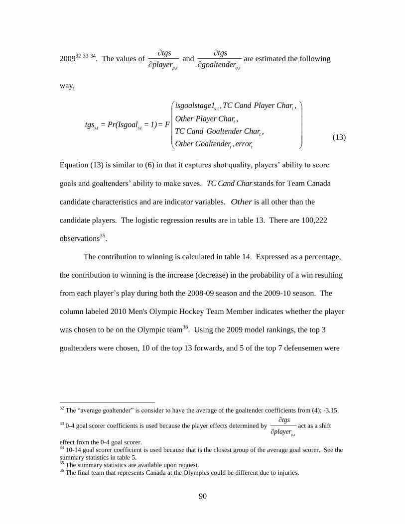
90
200932
33
34
. The values of ,p t
tgs
player
and
,q t
tgs
goaltender
are estimated the following
way,
, ,
s t t
t
s,t s,t
t
t t
isgoalstage1 TC Cand Player Char ,
Other Player Char ,tgs = Pr(Isgoal = 1)= F
TC Cand Goaltender Char ,
Other Goaltender , error
(13)
Equation (13) is similar to (6) in that it captures shot quality, players’ ability to score
goals and goaltenders’ ability to make saves. TC Cand Char stands for Team Canada
candidate characteristics and are indicator variables. Other is all other than the
candidate players. The logistic regression results are in table 13. There are 100,222
observations35
.
The contribution to winning is calculated in table 14. Expressed as a percentage,
the contribution to winning is the increase (decrease) in the probability of a win resulting
from each player’s play during both the 2008-09 season and the 2009-10 season. The
column labeled 2010 Men's Olympic Hockey Team Member indicates whether the player
was chosen to be on the Olympic team36
. Using the 2009 model rankings, the top 3
goaltenders were chosen, 10 of the top 13 forwards, and 5 of the top 7 defensemen were
32
The “average goaltender” is consider to have the average of the goaltender coefficients from (4); -3.15.
33 0-4 goal scorer coefficients is used because the player effects determined by
,p t
tgs
player
act as a shift
effect from the 0-4 goal scorer. 34
10-14 goal scorer coefficient is used because that is the closest group of the average goal scorer. See the
summary statistics in table 5. 35
The summary statistics are available upon request. 36
The final team that represents Canada at the Olympics could be different due to injuries.

91
chosen37
. Of course, the results can be used to measure individual player’s offensive and
defensive capabilities for game strategy decisions and player trends over time.
Concluding Comments
The underlying production process of contests is different than traditional
production theory because the output of a single firm is intrinsically connected to the
output of the other firms in the industry. Although improvements have been made in the
way of theoretical advancement in the study of contests, little supporting empirical work
currently exists. Functional forms are of particular interest because they impose
assumptions about the process that may significantly affect results.
In this paper, National Hockey League data is analyzed to estimate and test the fit
of the difference and ratio forms of the logistic model of the contest success function.
Using a multi-stage regression system, I created a statistic called theoretical goals scored
(tgs) and compared the prediction accuracy, goodness-of-fit, and specification of the
difference and ratio forms. Using the best form of the model is important because the
shape and marginal effects of each contest success function is different. Evidence
suggests that the ratio form is a better fit compared to the difference form. The ratio form
is of particular interest to sports economists that make simplifying assumptions in their
league models. The results of this article support their assumption that the talent
parameter in the ratio form is equal to one.
Since estimating the parameters of the contest success functions places value on
the inputs that contribute to winning, contribution to winning calculations are a possible
extension. An example is provided using the candidate players from the 2010 Canadian
37
I recognize that other factors are used in deciding team members than contribution to winning.
92
Men’s Olympic Hockey Team. Of the candidate players, Martin Brodeur (goaltender),
Jonathan Toews (forward), and Chris Pronger (defense) contributed the most to winning
at their respective positions during the first part of the 2009-10 NHL season. Each of
these players was selected to be a member of the 2010 Olympic Team. Cam Ward
(goaltender), Ryan Getzlaf (forward), and Mike Green (defense) were the top
contributors during the 2008-09 season. Ryan Getzlaf was the only one of these players
selected. Team managers can use the information enclosed in the regressions and
summary statistics for many different types of game and personnel decisions.
Extensions to this research are plentiful. Estimating other forms of the contest
success functions and testing their fit is an obvious route. Also, accounting for
heterogeneity across contestants may give insight into the factors that affect winning a
contest. Unobservable heterogeneities may exist in both a contestant’s ability to win
(intercept) and their response to the covariates (slope). It is beyond the scope of this
article, but the contribution to winning model can be enhanced by incorporating between
player effects and stage 1 and 2 of the regression can be modeled in different ways.
With the advances in the theoretical development of contest success function and
the wide range of production processes that have contest like behaviors, equal advances
in empirical modeling are important. This paper provides a jumping-off point for
researchers to build a foundation of empirical support describing the underlying process
of contests.

93
REFERENCES
Aiake, H. (1973). Information theory and an extension of the maximum likelihood
principle. In Second International Symposium on Information Theory, Ed. B. N.
Petrov and F. Czaki, 267-81.
Akademiai, K., Arbatskaya, M., and Mialon, H.M. (2009). Multi-activity contests.
Economic Theory, (forthcoming).
Baye, M., Kovenock, D., and de Vries, C.G. (1993). Rigging the lobbying process: An
application of the all-pay auction. American Economics Review 83:289–94.
Blavatskyy, P.R. (2008). Advances in the Theory of Contests and its Applications.
Institute for Empirical Research in Economics.
Banerjee, A., Swinnen, J.F.M., and Weersink, A. (2007). Skating on thin ice: Rule
changes and team strategies in the NHL. Canadian Journal of Economics 40(2):498-
514.
Clark, D. J. and Riis, C. (1996). Rank-Order Tournaments and Selection. Memorandum
no. 27, Department of Economics, University of Oslo, Oslo.
Clark, D.J. and Riis C. (1998). Contest success functions: an extension. Economic Theory
11:201-204.
Corchón, L.C. and Dahm, M. (2010). Foundations for contest success functions.
Economic Theory 42(1):89-98.
Cornes, R. and Hartley, R. (2003). Risk Aversion, Heterogeneity and Contests. Public
Choice, 117(1-2):1-25.
Dasgupta, P. and Stiglitz, J. (1980). Uncertainty, Industrial Structure, and the Speed of R
& D. Bell Journal of Economics 11:1-28.
Epstein, G.S and Nitzan. (2006) The Politics of Randomness. Social Choice and Welfare
27(2): 423-433.
Fort, R. (2006). Sports Economics. Second Edition. Upper Saddle River, NJ: Prentice all.
Fort, R. and Winfree, J. (2009). Sports Really are Different: The Contest Success
Function and the Supply of Talent. Review of Industrial Organization 34(1):69-80.
Green, J.R. and Stokey, N.L. (1983). A Comparison of Tournaments and Contracts. The
Journal of Political Economy 91(3):349-364.

94
Greene, W. (2003). Econometric Analysis. Fifth edition. Upper Saddle River, NJ:
Prentice Hall.
Hirshleifer, J. (1989). Conflict and rent-seeking success functions: Ratio vs. difference
models of relative success. Public Choice 63:101-12.
Holmstrom, B. (1982). Moral Hazard in Teams Bell. Journal of Economics 13:324-40.
Hosmer, D.W. and Lemshow S. (2000). Applied Logistic Regression. Second edition.
John Wiley & Sons, Inc.
Hwang, S. (2009). Contest Success Functions: Theory and Evidence. Working Paper.
Jia, H. (2008). A stochastic derivation of the ratio form of contest success functions.
Public Choice 135(3-4): 125-130.
Kesenne, S. (2005). Revenue sharing and competitive balance: Does the invariance
proposition hold? Journal of Sports Economics 5:98-106.
Kesenne, S. (2006). The win maximization model reconsidered: Flexible talent supply
and efficiency wages. Journal of Sports Economics 7:416–427.
Lazear, E.P. and Rosen, S. (2007). Rank-Order Tournaments as Optimum Labor
Contracts. The Journal of Political Economy 89(5):841-864.
Lee, T. and Wilde, L.L. (1980). Market Structure and Innovation: A Reformulation. The
Quarterly Journal of Economics 94(2):429-436.
Loury, G.C. (1979). Market Structure and Innovation. Quarterly Journal of Economics
93(3):395-410.
McFadden, D. (1974). Measurement of urban travel demand. Journal of Public
Economics 3(4):303-328.
Nalebuff, B. and Stiglitz, J. (1983). Prizes and Incentives: Toward a General Theory of
Compensation and Competition. Bell Journal of Economics 14 (1):21-43.
Nitzan, S. (1991). Collective rent dissipation. Economics Journal 101:1522-1534.
Rascher, D. (1997). A model of professional sports leagues. In: W. Hendricks (Ed.)
Advances in the Economics of Sport, volume 2:27-76.
Raftery, A.E. (1996). Approximate Bayes Factors and Accounting for Model Uncertainty
in Generalized Linear Regression Models. Biometrika 83:251-266.

95
Rai, B.K. and Sarin, R. (2007). Parametric Contest Success Functions. JENA Economic
Research Paper No. 2007-010.
Rosen, S. (1986) Prizes and Incentives in Elimination Tournaments. The American
Economic Review 76(4):701-715.
Schwarz, G. (1978). Estimating the dimension of a model. Ann. Statist. 6:461-464.
Scully, G.W. (1974). Pay and Performance in Major League Baseball. American
Economic Review 64:915-930.
Scully, G.W. (1989). The Business of Major League Baseball. Chicago: University of
Chicago Press.
Skaperdas, S. and Grofman, B. (1995). Modeling negative campaigning. Am. Polit. Sci.
Rev. 89:49-61.
Skaperdas, S. (1996). Contest Success Functions. Economic Theory 7(2):283-290.
Szymanski, S. (2003). The economic design of sporting contests. Journal of Economic
Literature 41:1137-1187.
Szymanski, S. (2004). Professional team sports are only a game: The Walrasian fixed-
supply conjecture model, contest-Nash equilibrium, and the invariance principle.
Journal of Sports Economics 5:111-126.
Szymanski, S. and Kesenne, S. (2004). Competitive balance and gate revenue sharing in
team sports. Journal of Industrial Economics 52:165–177.
Tullock, G. (1989). Efficient Rent Seeking. College Station, TX: Texas A&M University
Press.
Vuong, Q.H. (1989). Likelihood ratio test for model selection and non-nested
hypotheses. Econometrica 57:307-333.
Zimbalist, A. (1992). Baseball and Billion. New York: Basic Books.
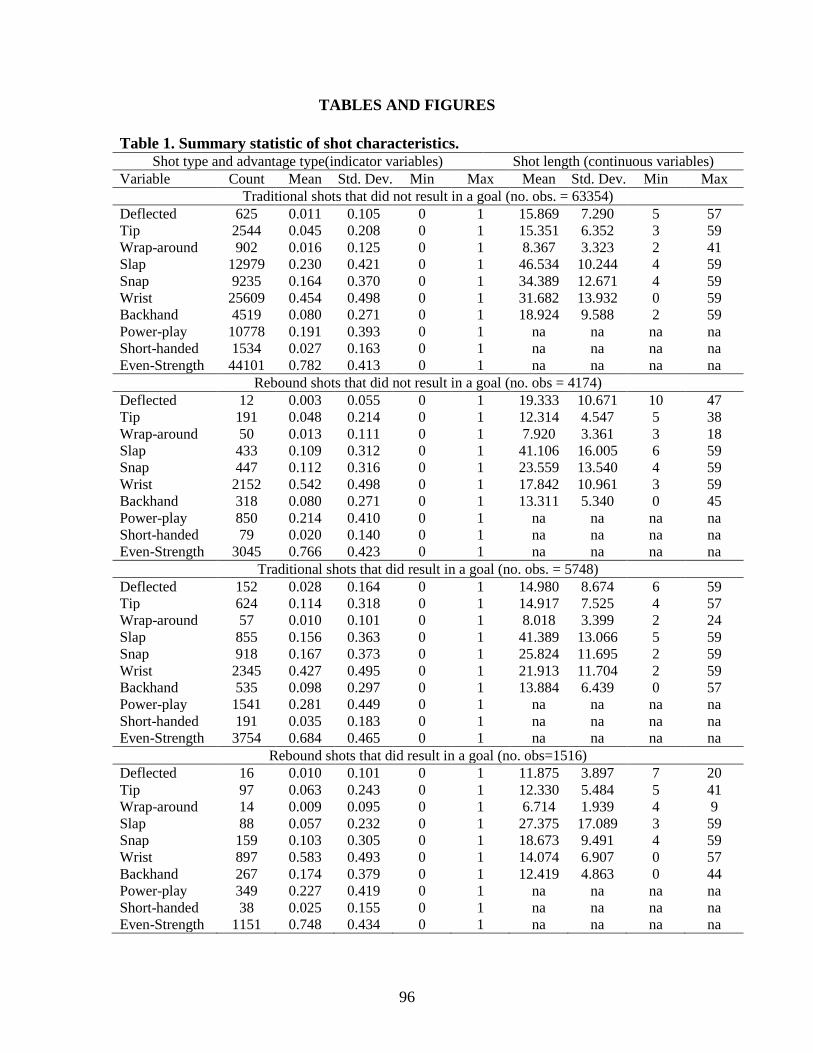
96
TABLES AND FIGURES
Table 1. Summary statistic of shot characteristics. Shot type and advantage type(indicator variables) Shot length (continuous variables)
Variable Count Mean Std. Dev. Min Max Mean Std. Dev. Min Max Traditional shots that did not result in a goal (no. obs. = 63354)
Deflected 625 0.011 0.105 0 1 15.869 7.290 5 57 Tip 2544 0.045 0.208 0 1 15.351 6.352 3 59 Wrap-around 902 0.016 0.125 0 1 8.367 3.323 2 41 Slap 12979 0.230 0.421 0 1 46.534 10.244 4 59 Snap 9235 0.164 0.370 0 1 34.389 12.671 4 59 Wrist 25609 0.454 0.498 0 1 31.682 13.932 0 59 Backhand 4519 0.080 0.271 0 1 18.924 9.588 2 59 Power-play 10778 0.191 0.393 0 1 na na na na Short-handed 1534 0.027 0.163 0 1 na na na na Even-Strength 44101 0.782 0.413 0 1 na na na na
Rebound shots that did not result in a goal (no. obs = 4174) Deflected 12 0.003 0.055 0 1 19.333 10.671 10 47 Tip 191 0.048 0.214 0 1 12.314 4.547 5 38 Wrap-around 50 0.013 0.111 0 1 7.920 3.361 3 18 Slap 433 0.109 0.312 0 1 41.106 16.005 6 59 Snap 447 0.112 0.316 0 1 23.559 13.540 4 59 Wrist 2152 0.542 0.498 0 1 17.842 10.961 3 59 Backhand 318 0.080 0.271 0 1 13.311 5.340 0 45 Power-play 850 0.214 0.410 0 1 na na na na Short-handed 79 0.020 0.140 0 1 na na na na Even-Strength 3045 0.766 0.423 0 1 na na na na
Traditional shots that did result in a goal (no. obs. = 5748) Deflected 152 0.028 0.164 0 1 14.980 8.674 6 59 Tip 624 0.114 0.318 0 1 14.917 7.525 4 57 Wrap-around 57 0.010 0.101 0 1 8.018 3.399 2 24 Slap 855 0.156 0.363 0 1 41.389 13.066 5 59 Snap 918 0.167 0.373 0 1 25.824 11.695 2 59 Wrist 2345 0.427 0.495 0 1 21.913 11.704 2 59 Backhand 535 0.098 0.297 0 1 13.884 6.439 0 57 Power-play 1541 0.281 0.449 0 1 na na na na Short-handed 191 0.035 0.183 0 1 na na na na Even-Strength 3754 0.684 0.465 0 1 na na na na
Rebound shots that did result in a goal (no. obs=1516) Deflected 16 0.010 0.101 0 1 11.875 3.897 7 20 Tip 97 0.063 0.243 0 1 12.330 5.484 5 41 Wrap-around 14 0.009 0.095 0 1 6.714 1.939 4 9 Slap 88 0.057 0.232 0 1 27.375 17.089 3 59 Snap 159 0.103 0.305 0 1 18.673 9.491 4 59 Wrist 897 0.583 0.493 0 1 14.074 6.907 0 57 Backhand 267 0.174 0.379 0 1 12.419 4.863 0 44 Power-play 349 0.227 0.419 0 1 na na na na Short-handed 38 0.025 0.155 0 1 na na na na Even-Strength 1151 0.748 0.434 0 1 na na na na

97
Figure 1a to 1f: Percentage of shots that resulted in goals by each length group for both actual and predicted values

98

99
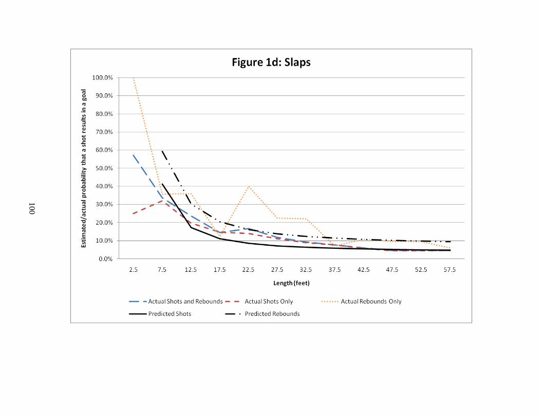
100

101
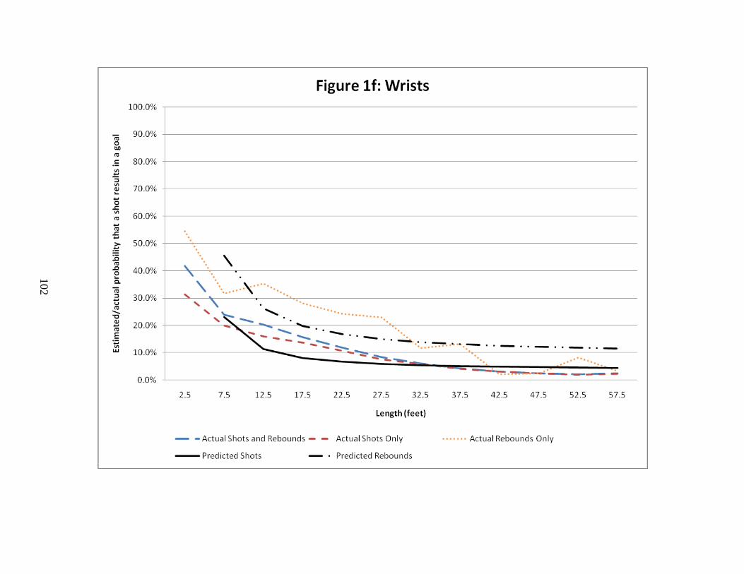
102

103
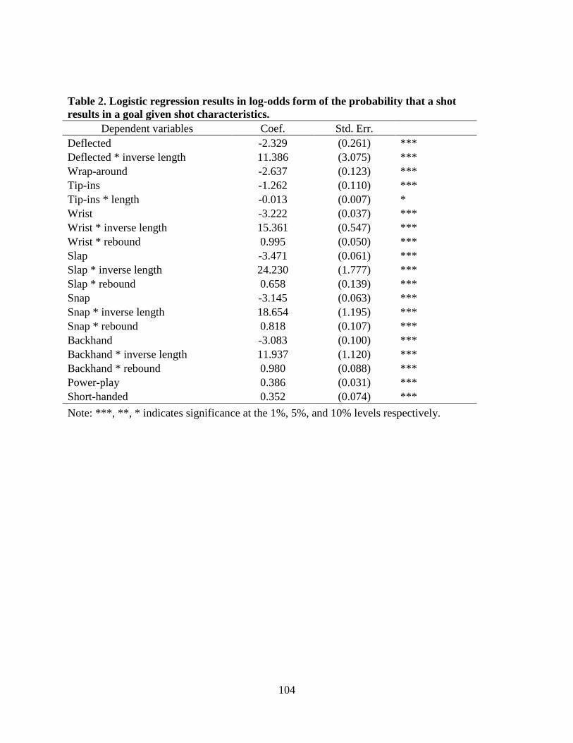
104
Table 2. Logistic regression results in log-odds form of the probability that a shot
results in a goal given shot characteristics.
Dependent variables Coef. Std. Err.
Deflected -2.329 (0.261) ***
Deflected * inverse length 11.386 (3.075) ***
Wrap-around -2.637 (0.123) ***
Tip-ins -1.262 (0.110) ***
Tip-ins * length -0.013 (0.007) *
Wrist -3.222 (0.037) ***
Wrist * inverse length 15.361 (0.547) ***
Wrist * rebound 0.995 (0.050) ***
Slap -3.471 (0.061) ***
Slap * inverse length 24.230 (1.777) ***
Slap * rebound 0.658 (0.139) ***
Snap -3.145 (0.063) ***
Snap * inverse length 18.654 (1.195) ***
Snap * rebound 0.818 (0.107) ***
Backhand -3.083 (0.100) ***
Backhand * inverse length 11.937 (1.120) ***
Backhand * rebound 0.980 (0.088) ***
Power-play 0.386 (0.031) ***
Short-handed 0.352 (0.074) ***
Note: ***, **, * indicates significance at the 1%, 5%, and 10% levels respectively.
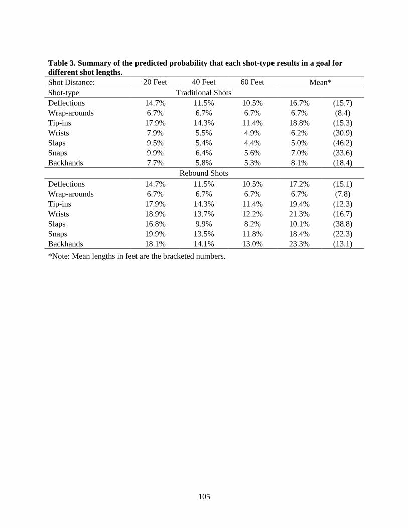
105
Table 3. Summary of the predicted probability that each shot-type results in a goal for
different shot lengths.
Shot Distance: 20 Feet 40 Feet 60 Feet Mean*
Shot-type Traditional Shots
Deflections 14.7% 11.5% 10.5% 16.7% (15.7)
Wrap-arounds 6.7% 6.7% 6.7% 6.7% (8.4)
Tip-ins 17.9% 14.3% 11.4% 18.8% (15.3)
Wrists 7.9% 5.5% 4.9% 6.2% (30.9)
Slaps 9.5% 5.4% 4.4% 5.0% (46.2)
Snaps 9.9% 6.4% 5.6% 7.0% (33.6)
Backhands 7.7% 5.8% 5.3% 8.1% (18.4)
Rebound Shots
Deflections 14.7% 11.5% 10.5% 17.2% (15.1)
Wrap-arounds 6.7% 6.7% 6.7% 6.7% (7.8)
Tip-ins 17.9% 14.3% 11.4% 19.4% (12.3)
Wrists 18.9% 13.7% 12.2% 21.3% (16.7)
Slaps 16.8% 9.9% 8.2% 10.1% (38.8)
Snaps 19.9% 13.5% 11.8% 18.4% (22.3)
Backhands 18.1% 14.1% 13.0% 23.3% (13.1)
*Note: Mean lengths in feet are the bracketed numbers.

106
Table 4. Logistic regression results in log-odds form and the marginal effects of the
probability that a shot results in a goals given the shot quality, and player and goaltender
characteristics.
Logistic Regression Marginal Effects
Dependent Variables Coef. Std. Err. Coef. Std. Err.
isgoalhat2008 6.253 (0.135) *** 0.493 (0.011) ***
5-9 goal scorer 0.704 (0.072) *** 0.068 (0.008) ***
10-14 goal scorer 0.883 (0.069) *** 0.089 (0.008) ***
15-19 goal scorer 1.027 (0.070) *** 0.110 (0.009) ***
20-24 goal scorer 1.112 (0.069) *** 0.123 (0.010) ***
25-29 goal scorer 1.197 (0.071) *** 0.140 (0.011) ***
30-34 goal scorer 1.248 (0.074) *** 0.151 (0.012) ***
35-39 goal scorer 1.277 (0.088) *** 0.162 (0.016) ***
40-44 goal scorer 1.335 (0.086) *** 0.173 (0.016) ***
45-49 goal scorer 1.404 (0.162) *** 0.191 (0.032) ***
50+ goal scorer 1.258 (0.147) *** 0.162 (0.027) ***
ANDERSON_CRAIG_2008 -4.088 (0.137) *** -0.089 (0.001) ***
AULD_ALEX_2008 -3.934 (0.127) *** -0.089 (0.001) ***
BACKSTROM_NIKLAS_2008 -4.009 (0.106) *** -0.093 (0.001) ***
BIRON_MARTIN_2008 -4.040 (0.113) *** -0.092 (0.001) ***
BISHOP_BEN_2008 -3.723 (0.313) *** -0.085 (0.001) ***
BOUCHER_BRIAN_2008 -4.220 (0.184) *** -0.087 (0.001) ***
BRODEUR_MARTIN_2008 -4.020 (0.138) *** -0.088 (0.001) ***
BRYZGALOV_ILJA_2008 -3.757 (0.099) *** -0.092 (0.001) ***
BUDAJ_PETER_2008 -3.742 (0.106) *** -0.090 (0.001) ***
CLEMMENSEN_SCOTT_2008 -3.949 (0.124) *** -0.089 (0.001) ***
CLIMIE_MATT_2008 -3.470 (0.327) *** -0.084 (0.001) ***
CONKLIN_TY_2008 -4.021 (0.138) *** -0.089 (0.001) ***
CURRY_JOHN_2008 -4.026 (0.430) *** -0.085 (0.001) ***
DANIS_YANN_2008 -3.937 (0.137) *** -0.088 (0.001) ***
DENIS_MARC_2008 -3.438 (1.193) *** -0.083 (0.004) ***
DIPIETRO_RICK_2008 -3.801 (0.303) *** -0.085 (0.001) ***
DROUINDESLAURIERS_JEFF_2008 -3.901 (0.219) *** -0.086 (0.001) ***
DUBIELEWICZ_WADE_2008 -3.615 (0.377) *** -0.084 (0.001) ***
ELLIOTT_BRIAN_2008 -3.766 (0.139) *** -0.087 (0.001) ***
ELLIS_DAN_2008 -3.811 (0.128) *** -0.088 (0.001) ***
ERSBERG_ERIK_2008 -3.729 (0.151) *** -0.087 (0.001) ***
FERNANDEZ_MANNY_2008 -3.938 (0.148) *** -0.088 (0.001) ***
FLEURY_MARCANDRE_2008 -3.953 (0.105) *** -0.093 (0.001) ***
GARON_MATHIEU_2008 -3.811 (0.165) *** -0.086 (0.001) ***
GERBER_MARTIN_2008 -3.806 (0.144) *** -0.087 (0.001) ***
GIGUERE_JEANSEBASTIEN_2008 -3.776 (0.114) *** -0.090 (0.001) ***
HALAK_JAROSLAV_2008 -4.045 (0.134) *** -0.089 (0.001) ***

107
Logistic Regression Marginal Effects
Dependent Variables Coef. Std. Err. Coef. Std. Err.
HARDING_JOSH_2008 -4.189 (0.201) *** -0.087 (0.001) ***
HEDBERG_JOHAN_2008 -3.705 (0.130) *** -0.087 (0.001) ***
HILLER_JONAS_2008 -4.053 (0.123) *** -0.090 (0.001) ***
HOWARD_JAMES_2008 -3.043 (0.554) *** -0.082 (0.003) ***
HUET_CRISTOBAL_2008 -3.974 (0.126) *** -0.089 (0.001) ***
JOHNSON_BRENT_2008 -3.820 (0.162) *** -0.087 (0.001) ***
JOSEPH_CURTIS_2008 -3.531 (0.168) *** -0.085 (0.001) ***
KHABIBULIN_NIKOLAI_2008 -4.055 (0.126) *** -0.090 (0.001) ***
KIPRUSOFF_MIIKKA_2008 -3.886 (0.101) *** -0.093 (0.001) ***
KOLZIG_OLAF_2008 -3.764 (0.231) *** -0.085 (0.001) ***
KRAHN_BRENT_2008 -2.232 (0.774) *** -0.076 (0.008) ***
LABARBERA_JASON_2008 -3.727 (0.140) *** -0.087 (0.001) ***
LACOSTA_DANIEL_2008 -4.906 (0.686) *** -0.086 (0.001) ***
LALIME_PATRICK_2008 -3.727 (0.145) *** -0.087 (0.001) ***
LECLAIRE_PASCAL_2008 -3.418 (0.178) *** -0.084 (0.001) ***
LEGACE_MANNY_2008 -3.538 (0.140) *** -0.086 (0.001) ***
LEHTONEN_KARI_2008 -3.940 (0.110) *** -0.091 (0.001) ***
LEIGHTON_MICHAEL_2008 -3.927 (0.172) *** -0.087 (0.001) ***
LUNDQVIST_HENRIK_2008 -4.068 (0.105) *** -0.094 (0.001) ***
LUONGO_ROBERTO_2008 -4.020 (0.112) *** -0.091 (0.001) ***
MACDONALD_JOEY_2008 -3.859 (0.110) *** -0.091 (0.001) ***
MANNINO_PETER_2008 -3.868 (0.375) *** -0.085 (0.001) ***
MASON_STEVE_2008 -3.958 (0.105) *** -0.092 (0.001) ***
MASON_CHRIS_2008 -3.959 (0.111) *** -0.091 (0.001) ***
MCELHINNEY_CURTIS_2008 -3.610 (0.220) *** -0.085 (0.001) ***
MCKENNA_MIKE_2008 -3.658 (0.175) *** -0.085 (0.001) ***
MILLER_RYAN_2008 -3.991 (0.108) *** -0.092 (0.001) ***
MONTOYA_AL_2008 -4.187 (0.441) *** -0.085 (0.001) ***
NABOKOV_EVGENI_2008 -3.962 (0.112) *** -0.092 (0.001) ***
NEUVIRTH_MICHAL_2008 -3.725 (0.356) *** -0.084 (0.001) ***
NIEMI_ANTTI_2008 -3.569 (0.406) *** -0.084 (0.002) ***
NIITTYMAKI_ANTERO_2008 -3.977 (0.137) *** -0.089 (0.001) ***
NORRENA_FREDRIK_2008 -3.454 (0.255) *** -0.084 (0.001) ***
OSGOOD_CHRIS_2008 -3.651 (0.114) *** -0.088 (0.001) ***
PAVELEC_ONDREJ_2008 -3.607 (0.195) *** -0.085 (0.001) ***
POGGE_JUSTIN_2008 -3.014 (0.211) *** -0.082 (0.001) ***
PRICE_CAREY_2008 -3.851 (0.108) *** -0.090 (0.001) ***
QUICK_JONATHAN_2008 -3.992 (0.124) *** -0.090 (0.001) ***
RAMO_KARRI_2008 -3.617 (0.133) *** -0.087 (0.001) ***
RAYCROFT_ANDREW_2008 -3.647 (0.131) *** -0.087 (0.001) ***
RINNE_PEKKA_2008 -4.030 (0.117) *** -0.091 (0.001) ***

108
Logistic Regression Marginal Effects
Dependent Variables Coef. Std. Err. Coef. Std. Err.
ROLOSON_DWAYNE_2008 -4.002 (0.107) *** -0.093 (0.001) ***
SABOURIN_DANY_2008 -3.824 (0.167) *** -0.086 (0.001) ***
SANFORD_CURTIS_2008 -3.875 (0.184) *** -0.086 (0.001) ***
SCHNEIDER_CORY_2008 -3.406 (0.246) *** -0.084 (0.001) ***
SMITH_MIKE_2008 -3.772 (0.114) *** -0.089 (0.001) ***
STEPHAN_TOBIAS_2008 -3.433 (0.218) *** -0.084 (0.001) ***
TELLQVIST_MIKAEL_2008 -3.867 (0.164) *** -0.087 (0.001) ***
THEODORE_JOSE_2008 -3.742 (0.104) *** -0.091 (0.001) ***
THOMAS_TIM_2008 -4.226 (0.118) *** -0.092 (0.001) ***
TORDJMAN_JOSH_2008 -3.354 (0.476) *** -0.083 (0.002) ***
TOSKALA_VESA_2008 -3.714 (0.106) *** -0.090 (0.001) ***
TURCO_MARTY_2008 -3.790 (0.098) *** -0.093 (0.001) ***
VARLAMOV_SIMEON_2008 -4.090 (0.336) *** -0.085 (0.001) ***
VOKOUN_TOMAS_2008 -4.093 (0.108) *** -0.093 (0.001) ***
WARD_CAM_2008 -4.092 (0.109) *** -0.093 (0.001) ***
WEEKES_KEVIN_2008 -3.951 (0.201) *** -0.086 (0.001) ***
Note: ***, **, * indicates significance at the 1%, 5%, and 10% levels respectively.
Note: Marginal effect of isgoalhatstage1 is taken at the mean=0.104.

109
Table 5. Summary statistics of isgoalhat and the player
characteristics
Variable Mean Std. Dev. Min Max
isgoalhatstage1 0.104 0.081 0.045 0.918
0-4 goal scorer 0.126 0.332 0.000 1.000
5-9 goal scorer 0.152 0.359 0.000 1.000
10-14 goal scorer 0.176 0.381 0.000 1.000
15-19 goal scorer 0.143 0.350 0.000 1.000
20-24 goal scorer 0.138 0.345 0.000 1.000
25-29 goal scorer 0.103 0.304 0.000 1.000
30-34 goal scorer 0.080 0.272 0.000 1.000
35-39 goal scorer 0.034 0.182 0.000 1.000
40-44 goal scorer 0.035 0.183 0.000 1.000
45-49 goal scorer 0.005 0.073 0.000 1.000
50+ goal scorer 0.008 0.091 0.000 1.000
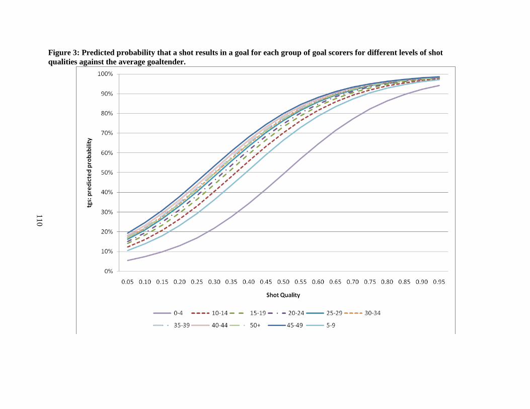
110
10
9 110
Figure 3: Predicted probability that a shot results in a goal for each group of goal scorers for different levels of shot
qualities against the average goaltender.

111
10
9 111
Figure 4: Predicted probability that a shot results in a goal for goaltenders Tim Thomas and Jose Theodore against
a 10-14 goal scorer.

112
10
9 112
Figure 5: Histogram of Theoretical Goals Scored: The predicted probability that a shot results in a goal given shot quality,
and player and goaltender characteristics.
05
10
15
De
nsity
0 .2 .4 .6 .8 1Theoretical Goals Scored

113
Table 6. Summary statistics of TGS and team 1 home game.
Mean Std. Dev. Min Max
Team 1 TGS 3.180 1.137 0.870 10.417
Team 2 TGS 3.158 1.021 0.933 7.391
Team 1 home game 0.500 0.500 0.000 1.000
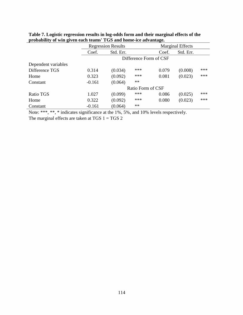
114
Table 7. Logistic regression results in log-odds form and their marginal effects of the
probability of win given each teams' TGS and home-ice advantage.
Regression Results Marginal Effects
Coef. Std. Err. Coef. Std. Err.
Difference Form of CSF
Dependent variables
Difference TGS 0.314 (0.034) *** 0.079 (0.008) ***
Home 0.323 (0.092) *** 0.081 (0.023) ***
Constant -0.161 (0.064) **
Ratio Form of CSF
Ratio TGS 1.027 (0.099) *** 0.086 (0.025) ***
Home 0.322 (0.092) *** 0.080 (0.023) ***
Constant -0.161 (0.064) **
Note: ***, **, * indicates significance at the 1%, 5%, and 10% levels respectively.
The marginal effects are taken at TGS 1 = TGS 2
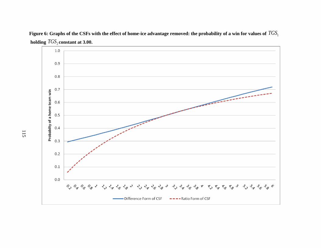
115
Figure 6: Graphs of the CSFs with the effect of home-ice advantage removed: the probability of a win for values of 1TGS
holding 2TGS constant at 3.00.

116
Figure 7: Marginal probability of winning of 1TGS holding 2TGS constant at 3.00. The marginal effects are calculated with the
effects of home-ice advantage removed.

117
Table 8. In-sample classification tables based.
Difference Form Ratio Form
Observed Observed
Classified Win Lose Total Win Lose Total
Win 339 186 525 339 187 526
Lose 216 321 537 216 320 536
Total 555 507 1062 555 507 1062
Classification Metrics Diff
Form Ratio Form
Sensitivity:(class wins & obs wins/total obs wins)% 61.1% 61.1%
Specificity: (class losses & obs losses/total obs losses)% 63.3% 63.1%
Positive predictive value: (class wins & obs wins/total class wins)% 64.6% 64.4%
Negative predictive value: (class losses & obs losses/total class losses)% 59.8% 59.7%
Correctly classified: ((class wins & obs wins + class losses & obs
losses)/total)% 62.1% 62.1%
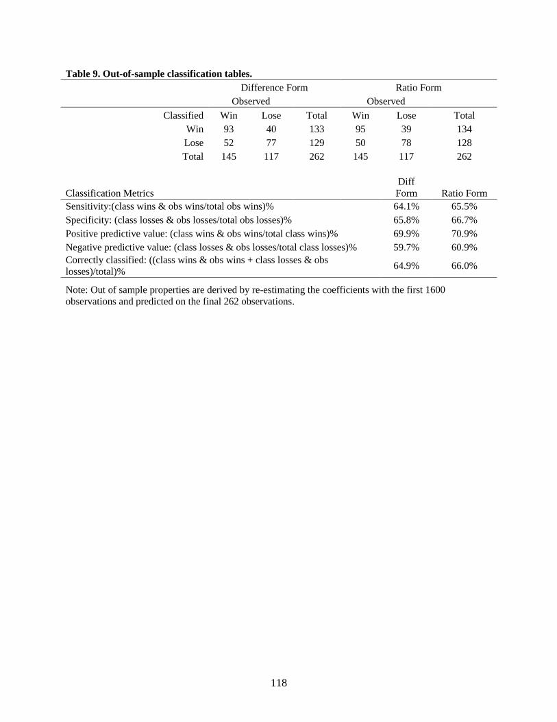
118
Table 9. Out-of-sample classification tables.
Difference Form Ratio Form
Observed Observed
Classified Win Lose Total Win Lose Total
Win 93 40 133 95 39 134
Lose 52 77 129 50 78 128
Total 145 117 262 145 117 262
Classification Metrics Diff
Form Ratio Form
Sensitivity:(class wins & obs wins/total obs wins)% 64.1% 65.5%
Specificity: (class losses & obs losses/total obs losses)% 65.8% 66.7%
Positive predictive value: (class wins & obs wins/total class wins)% 69.9% 70.9%
Negative predictive value: (class losses & obs losses/total class losses)% 59.7% 60.9%
Correctly classified: ((class wins & obs wins + class losses & obs
losses)/total)% 64.9% 66.0%
Note: Out of sample properties are derived by re-estimating the coefficients with the first 1600
observations and predicted on the final 262 observations.

119
Table 10. In-sample Hosmer-Lemeshow tables and test statistic calculation
Difference Form Ratio Form
Group Prob
Obs
win
Exp
win
Obs
loss
Exp
loss Total Group Prob
Obs
win
Exp
win
Obs
loss
Exp
loss Total
1 0.3337 30 29.9 77 77.1 107 1 0.318 31 28.7 76 78.3 107
2 0.3869 41 38.1 65 67.9 106 2 0.3761 43 37.2 63 68.8 106
3 0.4337 45 43.5 61 62.5 106 3 0.4241 40 42.7 66 63.3 106
4 0.4644 48 47.6 58 58.4 106 4 0.4619 54 47.1 52 58.9 106
5 0.4977 49 51.1 57 54.9 106 5 0.4979 45 50.9 61 55.1 106
6 0.5349 59 55.2 48 51.8 107 6 0.5356 62 55.2 45 51.8 107
7 0.5709 64 58.7 42 47.3 106 7 0.5722 61 58.8 45 47.2 106
8 0.6156 66 63 40 43 106 8 0.6183 66 63.3 40 42.7 106
9 0.668 75 67.7 31 38.3 106 9 0.6756 79 68.2 27 37.8 106
10 0.9333 78 77.5 28 28.5 106 10 0.8914 74 77.9 32 28.1 106
number of observations = 1062 number of observations = 1062
number of groups = 10 number of groups = 10
Hosmer-Lemeshow chi2(8) = 4.78 Hosmer-Lemeshow chi2(8) = 12.75
Prob > chi2 = 0.7806 Prob > chi2 = 0.1207

120
Table 11. Out-of-sample Hosmer-Lemeshow tables and test statistic calculation
Difference Form Ratio Form
Group Prob
Obs
win
Exp
win
Obs
loss
Exp
loss Total Group Prob
Obs
win
Exp
win
Obs
loss
Exp
loss Total
1 0.3269 9 7.6 18 19.4 27 1 0.3073 7 7.2 20 19.8 27
2 0.3796 7 9.2 19 16.8 26 2 0.3638 9 8.9 17 17.1 26
3 0.4339 12 10.5 14 15.5 26 3 0.4218 13 10.3 13 15.7 26
4 0.4681 15 11.7 11 14.3 26 4 0.4595 14 11.5 12 14.5 26
5 0.5024 11 12.5 15 13.5 26 5 0.5031 10 12.5 16 13.5 26
6 0.5432 16 14 11 13 27 6 0.5464 16 14.1 11 12.9 27
7 0.5832 16 14.6 10 11.4 26 7 0.5771 16 14.6 10 11.4 26
8 0.6206 19 15.7 7 10.3 26 8 0.6233 22 15.7 4 10.3 26
9 0.6508 21 16.4 5 9.6 26 9 0.6672 19 16.6 7 9.4 26
10 0.8673 19 18.6 7 7.4 26 10 0.8807 19 18.8 7 7.2 26
number of observations = 280 number of observations = 280
number of groups = 10 number of groups = 10
Hosmer-Lemeshow chi2(8) = 9.74 Hosmer-Lemeshow chi2(8) = 11.35
Prob > chi2 = 0.2841 Prob > chi2 = 0.1826

121
Table 12: McFadden’s LRI, AIC and BIC.
Model Ratio Form Difference Form Difference
McFadden's LRI 0.055 0.051 0.004
AIC 1.313 1.319 -0.005
BIC -13465.269 -13454.441 -10.828
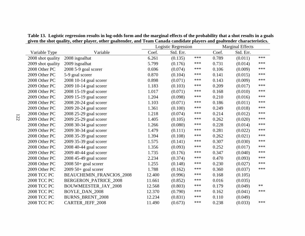
122
Table 13. Logistic regression results in log-odds form and the marginal effects of the probability that a shot results in a goals
given the shot quality, other player, other goaltender, and Team Canada candidate players and goaltender characteristics.
Logistic Regression Marginal Effects
Variable Type Variable Coef. Std. Err. Coef. Std. Err.
2008 shot quality 2008 isgoalhat 6.261 (0.135) *** 0.789 (0.011) ***
2009 shot quality 2009 isgoalhat 5.799 (0.176) *** 0.731 (0.014) ***
2008 Other PC 2008 5-9 goal scorer 0.696 (0.074) *** 0.106 (0.009) ***
2009 Other PC 5-9 goal scorer 0.870 (0.104) *** 0.141 (0.015) ***
2008 Other PC 2008 10-14 goal scorer 0.898 (0.071) *** 0.143 (0.009) ***
2009 Other PC 2009 10-14 goal scorer 1.183 (0.103) *** 0.209 (0.017) ***
2008 Other PC 2008 15-19 goal scorer 1.017 (0.071) *** 0.168 (0.010) ***
2009 Other PC 2009 15-19 goal scorer 1.204 (0.098) *** 0.210 (0.016) ***
2008 Other PC 2008 20-24 goal scorer 1.103 (0.071) *** 0.186 (0.011) ***
2009 Other PC 2009 20-24 goal scorer 1.361 (0.100) *** 0.249 (0.018) ***
2008 Other PC 2008 25-29 goal scorer 1.218 (0.074) *** 0.214 (0.012) ***
2009 Other PC 2009 25-29 goal scorer 1.405 (0.105) *** 0.262 (0.020) ***
2008 Other PC 2008 30-34 goal scorer 1.266 (0.080) *** 0.228 (0.014) ***
2009 Other PC 2009 30-34 goal scorer 1.479 (0.111) *** 0.281 (0.022) ***
2008 Other PC 2008 35-39 goal scorer 1.394 (0.108) *** 0.262 (0.021) ***
2009 Other PC 2009 35-39 goal scorer 1.575 (0.141) *** 0.307 (0.030) ***
2008 Other PC 2008 40-44 goal scorer 1.356 (0.093) *** 0.252 (0.017) ***
2009 Other PC 2009 40-44 goal scorer 1.735 (0.176) *** 0.347 (0.040) ***
2008 Other PC 2008 45-49 goal scorer 2.234 (0.374) *** 0.470 (0.093) ***
2008 Other PC 2008 50+ goal scorer 1.255 (0.148) *** 0.230 (0.027) ***
2009 Other PC 2009 50+ goal scorer 1.788 (0.162) *** 0.360 (0.037) ***
2008 TCC PC BEAUCHEMIN_FRANCIOS_2008 12.400 (0.996) *** 0.168 (0.105)
2008 TCC PC BERGERON_PATRICE_2008 11.661 (0.852) *** 0.016 (0.035)
2008 TCC PC BOUWMEESTER_JAY_2008 12.568 (0.803) *** 0.179 (0.049) **
2008 TCC PC BOYLE_DAN_2008 12.370 (0.790) *** 0.162 (0.041) ***
2008 TCC PC BURNS_BRENT_2008 12.234 (0.831) *** 0.110 (0.049)
2008 TCC PC CARTER_JEFF_2008 11.490 (0.673) *** 0.238 (0.033) ***

123
Logistic Regression Marginal Effects
Variable Type Variable Coef. Std. Err. Coef. Std. Err.
2008 TCC PC CLEARY_DANIEL_2008 12.065 (0.807) *** 0.079 (0.036)
2008 TCC PC CROSBY_SIDNEY_2008 12.230 (0.770) *** 0.214 (0.037) ***
2008 TCC PC DOAN_SHANE_2008 12.444 (0.775) *** 0.234 (0.040) ***
2008 TCC PC DOUGHTY_DREW_2008 12.538 (0.844) *** 0.130 (0.056)
2008 TCC PC GAGNE_SIMON_2008 12.167 (0.773) *** 0.200 (0.038) ***
2008 TCC PC GETZLAF_RYAN_2008 12.354 (0.773) *** 0.202 (0.036) ***
2008 TCC PC GREEN_MIKE_2008 12.548 (0.774) *** 0.291 (0.046) ***
2008 TCC PC HAMHUIS_DAN_2008 12.405 (0.992) *** -0.004 (0.045)
2008 TCC PC HEATLEY_DANY_2008 12.328 (0.769) *** 0.237 (0.039) ***
2008 TCC PC IGINLA_JAROME_2008 12.273 (0.772) *** 0.195 (0.035) ***
2008 TCC PC KEITH_DUNCAN_2008 12.492 (0.839) *** 0.121 (0.053)
2008 TCC PC LECAVALIER_VINCENT_2008 12.277 (0.772) *** 0.196 (0.035) ***
2008 TCC PC LUCIC_MILAN_2008 12.982 (0.795) *** 0.305 (0.059) ***
2008 TCC PC MARLEAU_PATRICK_2008 12.239 (0.770) *** 0.208 (0.035) ***
2008 TCC PC MCDONALD_ANDY_2008 12.473 (0.793) *** 0.230 (0.050) ***
2008 TCC PC MORROW_BRENDEN_2008 11.930 (0.874) *** 0.092 (0.056)
2008 TCC PC NASH_RICK_2008 12.404 (0.767) *** 0.246 (0.037) ***
2008 TCC PC NIEDERMAYER_SCOTT_2008 12.400 (0.798) *** 0.143 (0.042) **
2008 TCC PC PERRY_COREY_2008 12.218 (0.769) *** 0.183 (0.032) ***
2008 TCC PC PHANEUF_DION_2008 11.921 (0.818) *** 0.055 (0.036)
2008 TCC PC PRONGER_CHRIS_2008 12.406 (0.814) *** 0.144 (0.048) **
2008 TCC PC RICHARDS_MIKE_2008 12.342 (0.775) *** 0.211 (0.038) ***
2008 TCC PC ROBIDAS_STEPHANE_2008 12.429 (0.953) *** -0.001 (0.040)
2008 TCC PC ROY_DEREK_2008 12.284 (0.777) *** 0.187 (0.037) ***
2008 TCC PC SEABROOK_BRENT_2008 12.584 (0.845) *** 0.140 (0.058)
2008 TCC PC SHARP_PATRICK_2008 12.419 (0.783) *** 0.229 (0.045) ***
2008 TCC PC SPEZZA_JASON2008 11.907 (0.778) *** 0.109 (0.030) **
2008 TCC PC SMYTH_RYAN_2008 12.468 (0.773) *** 0.240 (0.039) ***
2008 TCC PC STLOUIS_MARTIN_2008 12.399 (0.775) *** 0.213 (0.038) ***
2008 TCC PC STAAL_ERIC_2008 11.916 (0.767) *** 0.146 (0.029) ***
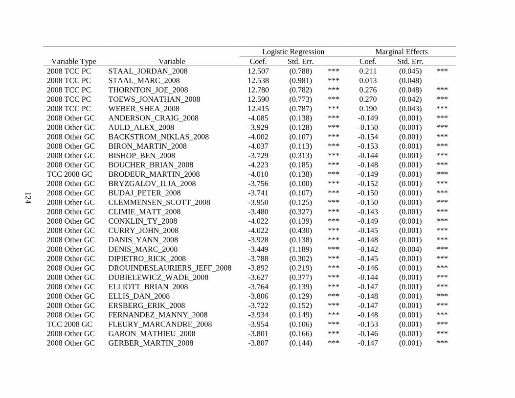
124
Logistic Regression Marginal Effects
Variable Type Variable Coef. Std. Err. Coef. Std. Err.
2008 TCC PC STAAL_JORDAN_2008 12.507 (0.788) *** 0.211 (0.045) ***
2008 TCC PC STAAL_MARC_2008 12.538 (0.981) *** 0.013 (0.048)
2008 TCC PC THORNTON_JOE_2008 12.780 (0.782) *** 0.276 (0.048) ***
2008 TCC PC TOEWS_JONATHAN_2008 12.590 (0.773) *** 0.270 (0.042) ***
2008 TCC PC WEBER_SHEA_2008 12.415 (0.787) *** 0.190 (0.043) ***
2008 Other GC ANDERSON_CRAIG_2008 -4.085 (0.138) *** -0.149 (0.001) ***
2008 Other GC AULD_ALEX_2008 -3.929 (0.128) *** -0.150 (0.001) ***
2008 Other GC BACKSTROM_NIKLAS_2008 -4.002 (0.107) *** -0.154 (0.001) ***
2008 Other GC BIRON_MARTIN_2008 -4.037 (0.113) *** -0.153 (0.001) ***
2008 Other GC BISHOP_BEN_2008 -3.729 (0.313) *** -0.144 (0.001) ***
2008 Other GC BOUCHER_BRIAN_2008 -4.223 (0.185) *** -0.148 (0.001) ***
TCC 2008 GC BRODEUR_MARTIN_2008 -4.010 (0.138) *** -0.149 (0.001) ***
2008 Other GC BRYZGALOV_ILJA_2008 -3.756 (0.100) *** -0.152 (0.001) ***
2008 Other GC BUDAJ_PETER_2008 -3.741 (0.107) *** -0.150 (0.001) ***
2008 Other GC CLEMMENSEN_SCOTT_2008 -3.950 (0.125) *** -0.150 (0.001) ***
2008 Other GC CLIMIE_MATT_2008 -3.480 (0.327) *** -0.143 (0.001) ***
2008 Other GC CONKLIN_TY_2008 -4.022 (0.139) *** -0.149 (0.001) ***
2008 Other GC CURRY_JOHN_2008 -4.022 (0.430) *** -0.145 (0.001) ***
2008 Other GC DANIS_YANN_2008 -3.928 (0.138) *** -0.148 (0.001) ***
2008 Other GC DENIS_MARC_2008 -3.449 (1.189) *** -0.142 (0.004) ***
2008 Other GC DIPIETRO_RICK_2008 -3.788 (0.302) *** -0.145 (0.001) ***
2008 Other GC DROUINDESLAURIERS_JEFF_2008 -3.892 (0.219) *** -0.146 (0.001) ***
2008 Other GC DUBIELEWICZ_WADE_2008 -3.627 (0.377) *** -0.144 (0.001) ***
2008 Other GC ELLIOTT_BRIAN_2008 -3.764 (0.139) *** -0.147 (0.001) ***
2008 Other GC ELLIS_DAN_2008 -3.806 (0.129) *** -0.148 (0.001) ***
2008 Other GC ERSBERG_ERIK_2008 -3.722 (0.152) *** -0.147 (0.001) ***
2008 Other GC FERNANDEZ_MANNY_2008 -3.934 (0.149) *** -0.148 (0.001) ***
TCC 2008 GC FLEURY_MARCANDRE_2008 -3.954 (0.106) *** -0.153 (0.001) ***
2008 Other GC GARON_MATHIEU_2008 -3.801 (0.166) *** -0.146 (0.001) ***
2008 Other GC GERBER_MARTIN_2008 -3.807 (0.144) *** -0.147 (0.001) ***

125
Logistic Regression Marginal Effects
Variable Type Variable Coef. Std. Err. Coef. Std. Err.
2008 Other GC GIGUERE_JEANSEBASTIEN_2008 -3.772 (0.115) *** -0.149 (0.001) ***
2008 Other GC HALAK_JAROSLAV_2008 -4.038 (0.135) *** -0.150 (0.001) ***
2008 Other GC HARDING_JOSH_2008 -4.189 (0.202) *** -0.147 (0.001) ***
2008 Other GC HEDBERG_JOHAN_2008 -3.705 (0.130) *** -0.147 (0.001) ***
2008 Other GC HILLER_JONAS_2008 -4.052 (0.123) *** -0.151 (0.001) ***
2008 Other GC HOWARD_JAMES_2008 -3.038 (0.555) *** -0.140 (0.003) ***
2008 Other GC HUET_CRISTOBAL_2008 -3.975 (0.126) *** -0.150 (0.001) ***
2008 Other GC JOHNSON_BRENT_2008 -3.818 (0.162) *** -0.147 (0.001) ***
2008 Other GC JOSEPH_CURTIS_2008 -3.517 (0.168) *** -0.144 (0.001) ***
2008 Other GC KHABIBULIN_NIKOLAI_2008 -4.051 (0.127) *** -0.150 (0.001) ***
2008 Other GC KIPRUSOFF_MIIKKA_2008 -3.886 (0.102) *** -0.154 (0.001) ***
2008 Other GC KOLZIG_OLAF_2008 -3.770 (0.231) *** -0.145 (0.001) ***
2008 Other GC KRAHN_BRENT_2008 -2.289 (0.809) *** -0.131 (0.008) ***
2008 Other GC LABARBERA_JASON_2008 -3.713 (0.141) *** -0.147 (0.001) ***
2008 Other GC LACOSTA_DANIEL_2008 -4.896 (0.689) *** -0.147 (0.001) ***
2008 Other GC LALIME_PATRICK_2008 -3.723 (0.146) *** -0.146 (0.001) ***
2008 Other GC LECLAIRE_PASCAL_2008 -3.409 (0.179) *** -0.143 (0.001) ***
2008 Other GC LEGACE_MANNY_2008 -3.539 (0.142) *** -0.146 (0.001) ***
2008 Other GC LEHTONEN_KARI_2008 -3.940 (0.111) *** -0.151 (0.001) ***
2008 Other GC LEIGHTON_MICHAEL_2008 -3.923 (0.172) *** -0.147 (0.001) ***
2008 Other GC LUNDQVIST_HENRIK_2008 -4.063 (0.106) *** -0.154 (0.001) ***
TCC 2008 GC LUONGO_ROBERTO_2008 -4.014 (0.113) *** -0.152 (0.001) ***
2008 Other GC MACDONALD_JOEY_2008 -3.856 (0.111) *** -0.151 (0.001) ***
2008 Other GC MANNINO_PETER_2008 -3.831 (0.376) *** -0.145 (0.001) ***
TCC 2008 GC MASON_STEVE_2008 -3.959 (0.107) *** -0.152 (0.001) ***
2008 Other GC MASON_CHRIS_2008 -3.954 (0.112) *** -0.152 (0.001) ***
2008 Other GC MCELHINNEY_CURTIS_2008 -3.579 (0.221) *** -0.144 (0.001) ***
2008 Other GC MCKENNA_MIKE_2008 -3.650 (0.177) *** -0.145 (0.001) ***
2008 Other GC MILLER_RYAN_2008 -3.991 (0.109) *** -0.152 (0.001) ***
2008 Other GC MONTOYA_AL_2008 -4.178 (0.441) *** -0.146 (0.001) ***
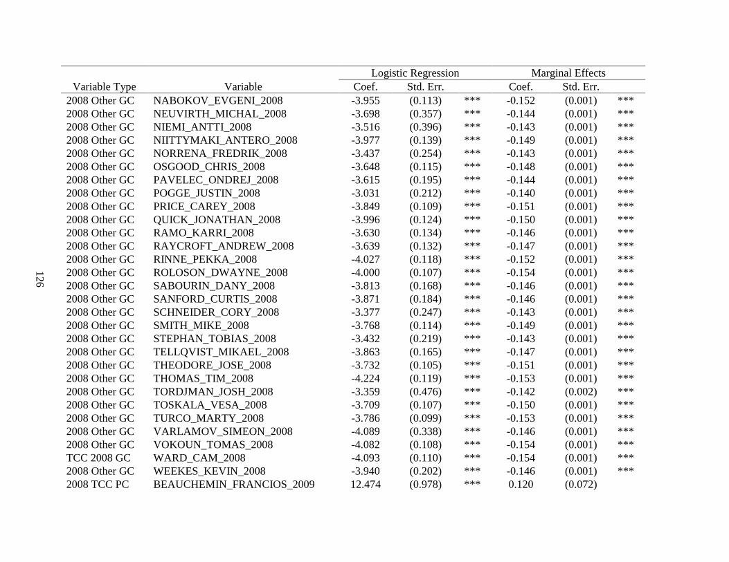
126
Logistic Regression Marginal Effects
Variable Type Variable Coef. Std. Err. Coef. Std. Err.
2008 Other GC NABOKOV_EVGENI_2008 -3.955 (0.113) *** -0.152 (0.001) ***
2008 Other GC NEUVIRTH_MICHAL_2008 -3.698 (0.357) *** -0.144 (0.001) ***
2008 Other GC NIEMI_ANTTI_2008 -3.516 (0.396) *** -0.143 (0.001) ***
2008 Other GC NIITTYMAKI_ANTERO_2008 -3.977 (0.139) *** -0.149 (0.001) ***
2008 Other GC NORRENA_FREDRIK_2008 -3.437 (0.254) *** -0.143 (0.001) ***
2008 Other GC OSGOOD_CHRIS_2008 -3.648 (0.115) *** -0.148 (0.001) ***
2008 Other GC PAVELEC_ONDREJ_2008 -3.615 (0.195) *** -0.144 (0.001) ***
2008 Other GC POGGE_JUSTIN_2008 -3.031 (0.212) *** -0.140 (0.001) ***
2008 Other GC PRICE_CAREY_2008 -3.849 (0.109) *** -0.151 (0.001) ***
2008 Other GC QUICK_JONATHAN_2008 -3.996 (0.124) *** -0.150 (0.001) ***
2008 Other GC RAMO_KARRI_2008 -3.630 (0.134) *** -0.146 (0.001) ***
2008 Other GC RAYCROFT_ANDREW_2008 -3.639 (0.132) *** -0.147 (0.001) ***
2008 Other GC RINNE_PEKKA_2008 -4.027 (0.118) *** -0.152 (0.001) ***
2008 Other GC ROLOSON_DWAYNE_2008 -4.000 (0.107) *** -0.154 (0.001) ***
2008 Other GC SABOURIN_DANY_2008 -3.813 (0.168) *** -0.146 (0.001) ***
2008 Other GC SANFORD_CURTIS_2008 -3.871 (0.184) *** -0.146 (0.001) ***
2008 Other GC SCHNEIDER_CORY_2008 -3.377 (0.247) *** -0.143 (0.001) ***
2008 Other GC SMITH_MIKE_2008 -3.768 (0.114) *** -0.149 (0.001) ***
2008 Other GC STEPHAN_TOBIAS_2008 -3.432 (0.219) *** -0.143 (0.001) ***
2008 Other GC TELLQVIST_MIKAEL_2008 -3.863 (0.165) *** -0.147 (0.001) ***
2008 Other GC THEODORE_JOSE_2008 -3.732 (0.105) *** -0.151 (0.001) ***
2008 Other GC THOMAS_TIM_2008 -4.224 (0.119) *** -0.153 (0.001) ***
2008 Other GC TORDJMAN_JOSH_2008 -3.359 (0.476) *** -0.142 (0.002) ***
2008 Other GC TOSKALA_VESA_2008 -3.709 (0.107) *** -0.150 (0.001) ***
2008 Other GC TURCO_MARTY_2008 -3.786 (0.099) *** -0.153 (0.001) ***
2008 Other GC VARLAMOV_SIMEON_2008 -4.089 (0.338) *** -0.146 (0.001) ***
2008 Other GC VOKOUN_TOMAS_2008 -4.082 (0.108) *** -0.154 (0.001) ***
TCC 2008 GC WARD_CAM_2008 -4.093 (0.110) *** -0.154 (0.001) ***
2008 Other GC WEEKES_KEVIN_2008 -3.940 (0.202) *** -0.146 (0.001) ***
2008 TCC PC BEAUCHEMIN_FRANCIOS_2009 12.474 (0.978) *** 0.120 (0.072)

127
Logistic Regression Marginal Effects
Variable Type Variable Coef. Std. Err. Coef. Std. Err.
2008 TCC PC BERGERON_PATRICE_2009 12.562 (0.883) *** 0.247 (0.059) ***
2008 TCC PC BOUWMEESTER_JAY_2009 13.048 (1.126) *** 0.066 (0.073)
2008 TCC PC BOYLE_DAN_2009 12.519 (0.905) *** -0.010 (0.026)
2008 TCC PC BURNS_BRENT_2009 11.687 (1.306) *** -0.005 (0.076)
2008 TCC PC CARTER_JEFF_2009 12.149 (0.875) *** 0.163 (0.045) **
2008 TCC PC CLEARY_DANIEL_2009 12.385 (0.925) *** 0.205 (0.072) **
2008 TCC PC CROSBY_SIDNEY_2009 12.595 (0.845) *** 0.360 (0.049) ***
2008 TCC PC DOAN_SHANE_2009 12.091 (0.898) *** -0.053 (0.017) *
2008 TCC PC DOUGHTY_DREW_2009 13.342 (0.917) *** 0.119 (0.053)
2008 TCC PC GAGNE_SIMON_2009 11.262 (1.077) *** 0.003 (0.055)
2008 TCC PC GETZLAF_RYAN_2009 12.523 (0.906) *** 0.238 (0.069) **
2008 TCC PC GREEN_MIKE_2009 12.829 (0.904) *** 0.312 (0.078) ***
2008 TCC PC HAMHUIS_DAN_2009 13.174 (0.981) *** 0.276 (0.107) *
2008 TCC PC HEATLEY_DANY_2009 14.157 (0.951) *** 0.304 (0.057) ***
2008 TCC PC IGINLA_JAROME_2009 12.646 (0.868) *** 0.320 (0.061) ***
2008 TCC PC KEITH_DUNCAN_2009 12.901 (0.919) *** 0.042 (0.039)
2008 TCC PC LECAVALIER_VINCENT_2009 12.215 (0.907) *** 0.168 (0.059) *
2008 TCC PC LUCIC_MILAN_2009 13.284 (1.128) *** 0.381 (0.180)
2008 TCC PC MARLEAU_PATRICK_2009 12.551 (0.860) *** 0.349 (0.061) ***
2008 TCC PC MCDONALD_ANDY_2009 12.819 (0.877) *** 0.320 (0.063) ***
2008 TCC PC MORROW_BRENDEN_2009 12.250 (0.912) *** 0.185 (0.064) **
2008 TCC PC NASH_RICK_2009 12.520 (0.861) *** 0.265 (0.049) ***
2008 TCC PC NIEDERMAYER_SCOTT_2009 12.574 (0.974) *** 0.140 (0.075)
2008 TCC PC PERRY_COREY_2009 12.236 (0.877) *** 0.198 (0.051) ***
2008 TCC PC PHANEUF_DION_2009 12.435 (0.949) *** 0.177 (0.076)
2008 TCC PC PRONGER_CHRIS_2009 12.723 (0.986) *** 0.243 (0.102) *
2008 TCC PC RICHARDS_MIKE_2009 12.642 (0.875) *** 0.295 (0.061) ***
2008 TCC PC ROBIDAS_STEPHANE_2009 12.590 (0.922) *** -0.001 (0.031)
2008 TCC PC ROY_DEREK_2009 12.396 (0.912) *** -0.024 (0.025)
2008 TCC PC SEABROOK_BRENT_2009 12.428 (1.010) *** 0.111 (0.077)
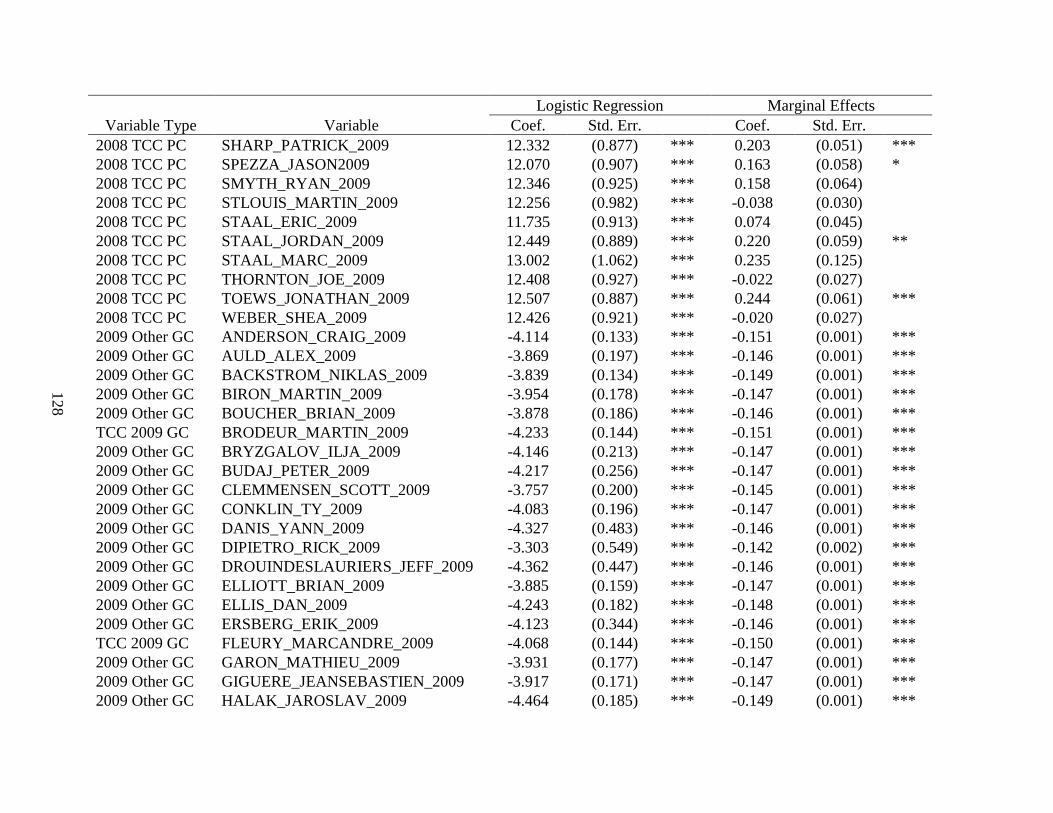
128
Logistic Regression Marginal Effects
Variable Type Variable Coef. Std. Err. Coef. Std. Err.
2008 TCC PC SHARP_PATRICK_2009 12.332 (0.877) *** 0.203 (0.051) ***
2008 TCC PC SPEZZA_JASON2009 12.070 (0.907) *** 0.163 (0.058) *
2008 TCC PC SMYTH_RYAN_2009 12.346 (0.925) *** 0.158 (0.064)
2008 TCC PC STLOUIS_MARTIN_2009 12.256 (0.982) *** -0.038 (0.030)
2008 TCC PC STAAL_ERIC_2009 11.735 (0.913) *** 0.074 (0.045)
2008 TCC PC STAAL_JORDAN_2009 12.449 (0.889) *** 0.220 (0.059) **
2008 TCC PC STAAL_MARC_2009 13.002 (1.062) *** 0.235 (0.125)
2008 TCC PC THORNTON_JOE_2009 12.408 (0.927) *** -0.022 (0.027)
2008 TCC PC TOEWS_JONATHAN_2009 12.507 (0.887) *** 0.244 (0.061) ***
2008 TCC PC WEBER_SHEA_2009 12.426 (0.921) *** -0.020 (0.027)
2009 Other GC ANDERSON_CRAIG_2009 -4.114 (0.133) *** -0.151 (0.001) ***
2009 Other GC AULD_ALEX_2009 -3.869 (0.197) *** -0.146 (0.001) ***
2009 Other GC BACKSTROM_NIKLAS_2009 -3.839 (0.134) *** -0.149 (0.001) ***
2009 Other GC BIRON_MARTIN_2009 -3.954 (0.178) *** -0.147 (0.001) ***
2009 Other GC BOUCHER_BRIAN_2009 -3.878 (0.186) *** -0.146 (0.001) ***
TCC 2009 GC BRODEUR_MARTIN_2009 -4.233 (0.144) *** -0.151 (0.001) ***
2009 Other GC BRYZGALOV_ILJA_2009 -4.146 (0.213) *** -0.147 (0.001) ***
2009 Other GC BUDAJ_PETER_2009 -4.217 (0.256) *** -0.147 (0.001) ***
2009 Other GC CLEMMENSEN_SCOTT_2009 -3.757 (0.200) *** -0.145 (0.001) ***
2009 Other GC CONKLIN_TY_2009 -4.083 (0.196) *** -0.147 (0.001) ***
2009 Other GC DANIS_YANN_2009 -4.327 (0.483) *** -0.146 (0.001) ***
2009 Other GC DIPIETRO_RICK_2009 -3.303 (0.549) *** -0.142 (0.002) ***
2009 Other GC DROUINDESLAURIERS_JEFF_2009 -4.362 (0.447) *** -0.146 (0.001) ***
2009 Other GC ELLIOTT_BRIAN_2009 -3.885 (0.159) *** -0.147 (0.001) ***
2009 Other GC ELLIS_DAN_2009 -4.243 (0.182) *** -0.148 (0.001) ***
2009 Other GC ERSBERG_ERIK_2009 -4.123 (0.344) *** -0.146 (0.001) ***
TCC 2009 GC FLEURY_MARCANDRE_2009 -4.068 (0.144) *** -0.150 (0.001) ***
2009 Other GC GARON_MATHIEU_2009 -3.931 (0.177) *** -0.147 (0.001) ***
2009 Other GC GIGUERE_JEANSEBASTIEN_2009 -3.917 (0.171) *** -0.147 (0.001) ***
2009 Other GC HALAK_JAROSLAV_2009 -4.464 (0.185) *** -0.149 (0.001) ***

129
Logistic Regression Marginal Effects
Variable Type Variable Coef. Std. Err. Coef. Std. Err.
2009 Other GC HARDING_JOSH_2009 -3.791 (0.217) *** -0.145 (0.001) ***
2009 Other GC HEDBERG_JOHAN_2009 -4.225 (0.171) *** -0.148 (0.001) ***
2009 Other GC HILLER_JONAS_2009 -4.173 (0.150) *** -0.150 (0.001) ***
2009 Other GC HOWARD_JAMES_2009 -3.886 (0.250) *** -0.145 (0.001) ***
2009 Other GC HUET_CRISTOBAL_2009 -4.067 (0.158) *** -0.149 (0.001) ***
2009 Other GC JOHNSON_BRENT_2009 -4.194 (0.229) *** -0.147 (0.001) ***
2009 Other GC KHABIBULIN_NIKOLAI_2009 -3.988 (0.173) *** -0.147 (0.001) ***
2009 Other GC KIPRUSOFF_MIIKKA_2009 -4.304 (0.145) *** -0.152 (0.001) ***
2009 Other GC LABARBERA_JASON_2009 -4.261 (0.253) *** -0.147 (0.001) ***
2009 Other GC LALIME_PATRICK_2009 -4.064 (0.255) *** -0.146 (0.001) ***
2009 Other GC LECLAIRE_PASCAL_2009 -3.906 (0.166) *** -0.147 (0.001) ***
2009 Other GC LEGACE_MANNY_2009 -4.070 (0.204) *** -0.147 (0.001) ***
2009 Other GC LEIGHTON_MICHAEL_2009 -3.996 (0.194) *** -0.147 (0.001) ***
2009 Other GC LUNDQVIST_HENRIK_2009 -4.248 (0.139) *** -0.151 (0.001) ***
TCC 2009 GC LUONGO_ROBERTO_2009 -4.203 (0.146) *** -0.151 (0.001) ***
2009 Other GC MACDONALD_JOEY_2009 -3.768 (0.273) *** -0.145 (0.001) ***
TCC 2009 GC MASON_STEVE_2009 -3.801 (0.137) *** -0.148 (0.001) ***
2009 Other GC MASON_CHRIS_2009 -4.033 (0.148) *** -0.149 (0.001) ***
2009 Other GC MCELHINNEY_CURTIS_2009 -3.752 (0.258) *** -0.145 (0.001) ***
2009 Other GC MILLER_RYAN_2009 -4.412 (0.151) *** -0.151 (0.001) ***
2009 Other GC NABOKOV_EVGENI_2009 -4.297 (0.146) *** -0.152 (0.001) ***
2009 Other GC NEUVIRTH_MICHAL_2009 -4.057 (0.234) *** -0.146 (0.001) ***
2009 Other GC NIEMI_ANTTI_2009 -4.229 (0.217) *** -0.147 (0.001) ***
2009 Other GC NIITTYMAKI_ANTERO_2009 -4.182 (0.174) *** -0.148 (0.001) ***
2009 Other GC OSGOOD_CHRIS_2009 -3.808 (0.177) *** -0.146 (0.001) ***
2009 Other GC PAVELEC_ONDREJ_2009 -4.031 (0.151) *** -0.149 (0.001) ***
2009 Other GC PRICE_CAREY_2009 -4.072 (0.151) *** -0.149 (0.001) ***
2009 Other GC QUICK_JONATHAN_2009 -3.988 (0.142) *** -0.150 (0.001) ***
2009 Other GC RAYCROFT_ANDREW_2009 -3.910 (0.277) *** -0.145 (0.001) ***
2009 Other GC RINNE_PEKKA_2009 -4.047 (0.153) *** -0.149 (0.001) ***

130
Logistic Regression Marginal Effects
Variable Type Variable Coef. Std. Err. Coef. Std. Err.
2009 Other GC ROLOSON_DWAYNE_2009 -4.071 (0.145) *** -0.150 (0.001) ***
2009 Other GC SCHNEIDER_CORY_2009 -4.387 (0.598) *** -0.146 (0.001) ***
2009 Other GC SMITH_MIKE_2009 -3.949 (0.150) *** -0.148 (0.001) ***
2009 Other GC THEODORE_JOSE_2009 -3.887 (0.164) *** -0.147 (0.001) ***
2009 Other GC THOMAS_TIM_2009 -4.113 (0.158) *** -0.149 (0.001) ***
2009 Other GC TOSKALA_VESA_2009 -3.708 (0.163) *** -0.146 (0.001) ***
2009 Other GC TURCO_MARTY_2009 -3.983 (0.141) *** -0.149 (0.001) ***
2009 Other GC VOKOUN_TOMAS_2009 -4.219 (0.138) *** -0.151 (0.001) ***
TCC 2009 GC WARD_CAM_2009 -4.080 (0.150) *** -0.149 (0.001) ***
Note: ***, **, * indicates significance at the 1%, 5%, and 10% levels respectively.
Note: Marginal effect of isgoalhatstage1 is taken at the mean=0.104.
Note: TCC stands for Team Canada candidate, PC stands for player characteristics, and GC stands for goaltender characteristics.

131
Table 14. Summary of contribution to winning statistics and percentage of contribution to winning calculation.
2008
Rank 2009
Rank
2010 Men's
Olympic
Hockey
Team
Member TCC Player 2008
TGSF 2008
TGSA
2008 Marg.
Prob. of
Scoring/Saving 2008 %
of CW 2009
TGSF 2009
TGSA
2009 Marg.
Prob. of
Scoring/Saving 2009 %
of CW
Goaltenders
5 1 Y Martin Brodeur NA NA -0.149 1.28% NA NA -0.151 1.30%
4 2 Y Roberto Luongo NA NA -0.152 1.31% NA NA -0.151 1.29%
2 3 Y Marc-Andre Fleury NA NA -0.153 1.32% NA NA -0.150 1.29%
1 4 N Cam Ward NA NA -0.154 1.32% NA NA -0.149 1.28%
3 5 N Steve Mason NA NA -0.152 1.31% NA NA -0.148 1.27%
Forwards
7 1 Y Jonathan Toews 0.371 0.368 0.270 0.89% 0.444 0.318 0.244 2.02%
3 2 Y Patrick Marleau 0.491 0.441 0.208 1.31% 0.537 0.492 0.349 1.99%
17 3 Y Sidney Crosby 0.417 0.487 0.214 0.17% 0.469 0.465 0.360 1.48%
22 4 Y Patrice Bergeron 0.289 0.309 0.000 -0.17% 0.392 0.326 0.247 1.40%
18 5 N Patrick Sharp 0.366 0.431 0.229 0.16% 0.425 0.363 0.203 1.28%
14 6 Y Dany Heatley 0.379 0.438 0.237 0.27% 0.491 0.504 0.304 1.17%
8 7 Y Rick Nash 0.414 0.414 0.246 0.88% 0.436 0.418 0.265 1.16%
26 8 Y Brenden Morrow 0.280 0.388 0.000 -0.92% 0.375 0.350 0.185 0.82%
11 9 Y Mike Richards 0.419 0.453 0.211 0.46% 0.447 0.485 0.295 0.81%
6 10 N Ryan Smyth 0.457 0.425 0.240 1.22% 0.397 0.365 0.158 0.81%
1 11 Y Ryan Getzlaf 0.489 0.418 0.202 1.47% 0.504 0.531 0.238 0.80%
4 12 Y Corey Perry 0.476 0.418 0.183 1.25% 0.520 0.536 0.198 0.75%
21 13 N Jason Spezza 0.370 0.427 0.109 -0.15% 0.475 0.472 0.163 0.68%
16 14 N Jeff Carter 0.415 0.491 0.238 0.20% 0.511 0.519 0.163 0.65%
19 15 N Jordan Staal 0.303 0.355 0.211 0.10% 0.368 0.401 0.220 0.42%
24 16 N Daniel Cleary 0.358 0.397 0.000 -0.34% 0.372 0.400 0.205 0.41%
20 17 Y Jarome Iginla 0.443 0.520 0.195 0.08% 0.402 0.492 0.320 0.33%
25 18 N Shane Doan 0.336 0.470 0.234 -0.47% 0.419 0.361 -0.053 0.30%

132
2008
Rank 2009
Rank
2010 Men's
Olympic
Hockey
Team
Member TCC Player 2008
TGSF 2008
TGSA
2008 Marg.
Prob. of
Scoring/Saving 2008 %
of CW 2009
TGSF 2009
TGSA
2009 Marg.
Prob. of
Scoring/Saving 2009 %
of CW
9 19 N Simon Gagne 0.399 0.387 0.200 0.79% 0.402 0.411 0.000 -0.08%
15 20 N Andy McDonald 0.313 0.355 0.230 0.26% 0.359 0.488 0.320 -0.12%
13 21 N Vincent Lecavalier 0.370 0.411 0.196 0.27% 0.369 0.455 0.168 -0.21%
2 22 Y Joe Thornton 0.480 0.450 0.276 1.40% 0.494 0.519 0.000 -0.21%
10 23 N Martin St. Louis 0.398 0.402 0.213 0.69% 0.364 0.401 0.000 -0.31%
5 24 Y Eric Staal 0.518 0.451 0.146 1.23% 0.497 0.535 0.000 -0.32%
12 25 N Derek Roy 0.359 0.383 0.187 0.37% 0.361 0.422 0.000 -0.53%
23 26 N Milan Lucic 0.302 0.419 0.305 -0.22% 0.225 0.362 0.000 -1.18%
Defense
4 1 Y Chris Pronger 0.416 0.493 0.144 -0.15% 0.543 0.505 0.243 1.47%
15 2 N Dan Hamhuis 0.433 0.586 0.000 -1.32% 0.562 0.587 0.276 1.12%
14 3 N Brent Burns 0.333 0.472 0.000 -1.20% 0.480 0.415 0.000 0.56%
8 4 Y Duncan Keith 0.559 0.600 0.000 -0.35% 0.569 0.509 0.000 0.52%
13 5 Y Drew Doughty 0.391 0.496 0.000 -0.91% 0.461 0.414 0.000 0.40%
5 6 Y Brent Seabrook 0.479 0.505 0.000 -0.22% 0.510 0.468 0.000 0.37%
1 7 N Mike Green 0.518 0.485 0.291 1.58% 0.450 0.565 0.312 0.21%
2 8 Y Dan Boyle 0.511 0.471 0.162 1.05% 0.562 0.548 0.000 0.12%
6 9 N Stephane Robidas 0.433 0.470 0.000 -0.32% 0.445 0.437 0.000 0.07%
16 10 N Francois Beauchemin 0.438 0.600 0.000 -1.39% 0.538 0.532 0.000 0.05%
3 11 Y Shea Weber 0.502 0.536 0.190 0.54% 0.488 0.521 0.000 -0.29%
7 12 Y Scott Niedermayer 0.433 0.535 0.143 -0.34% 0.486 0.606 0.000 -1.03%
10 13 N Dion Phaneuf 0.542 0.592 0.000 -0.44% 0.418 0.566 0.000 -1.27%
11 14 N Jay Bouwmeester 0.424 0.578 0.179 -0.68% 0.365 0.514 0.000 -1.28%
12 15 N Robyn Regehr 0.411 0.492 0.000 -0.69% 0.378 0.542 0.000 -1.41%
9 16 N Marc Staal 0.495 0.539 0.000 -0.38% 0.391 0.578 0.000 -1.61%