Efficient Estimation of Bayesian VARMAs with

Time-Varying Coefficients

Joshua C.C. Chan∗

Economics Discipline Group,

University of Technology Sydney

Eric Eisenstat†

School of Economics,

The University of Queensland

March 2017

Abstract

Empirical work in macroeconometrics has been mostly restricted to using VARs,even though there are strong theoretical reasons to consider general VARMAs. Anumber of articles in the last two decades have conjectured that this is because es-timation of VARMAs is perceived to be challenging and proposed various ways tosimplify it. Nevertheless, VARMAs continue to be largely dominated by VARs, par-ticularly in terms of developing useful extensions. We address these computationalchallenges with a Bayesian approach. Specifically, we develop a Gibbs sampler forthe basic VARMA, and demonstrate how it can be extended to models with time-varying VMA coefficients and stochastic volatility. We illustrate the methodologythrough a macroeconomic forecasting exercise. We show that in a class of modelswith stochastic volatility, VARMAs produce better density forecasts than VARs,particularly for short forecast horizons.

Keywords: state space, stochastic volatility, factor model, macroeconomic forecast-ing, density forecast

JEL codes: C11, C32, C53

∗Joshua Chan would also like to acknowledge financial support by the Australian Research Councilvia a Discovery Early Career Researcher Award (DE150100795).

†Corresponding author: School of Economics, The University of Queensland, Level 6, Colin ClarkBuilding (39), St. Lucia, Brisbane Qld 4072 (Australia), e.eisenstat@uq.edu.au.

1 Introduction

Vector autoregressive moving average (VARMA) models have long been considered anappropriate framework for modeling covariance stationary time series. As is well known,by the Wold decomposition theorem, any covariance stationary time series has an infinitemoving average representation. Whenever this is characterized by a rational transferfunction, the multivariate series can be exactly represented by a finite-order VARMAmodel. When the transfer function is irrational, the VARMA specification can be usedto provide an arbitrarily close approximation (Lutkepohl and Poskitt, 1996).

However, in most empirical work, only purely autoregressive models are considered. Infact, since the seminal work of Sims (1980), VARs have become the most prominentapproach in empirical macroeconometrics. This is in spite of long-standing criticismsof VARs, especially with short lag orders, as being theoretically deficient for macroeco-nomic applications. There are two main theoretical drawbacks of VARs in this context:first, linearized DSGE models typically result in VARMAs, not VARs (e.g., Cooley andDwyer, 1998; Yang, 2005; Fernandez-Villaverde, Rubio-Ramırez, Sargent, and Watson,2007; Leeper, Walker, and Yang, 2008). Second, even if a particular set of variables canbe adequately described by a VAR, any linear combination, temporal aggregation, orsubsets of these variables will follow a VARMA process.

Over the past two decades, a number of authors (e.g., Lutkepohl and Poskitt, 1996;Lutkepohl and Claessen, 1997; Athanasopoulos and Vahid, 2008; Athanasopoulos, Poskitt,and Vahid, 2012; Dufour and Stevanovic, 2013; Dufour and Pelletier, 2014; Kascha andTrenkler, 2014; Poskitt, 2016) have pointed out this unfortunate phenomenon and variousapproaches have been proposed aimed at making VARMAs accessible to applied macroe-conomists. Nevertheless, VARs continue to dominate in this field. One possible reasonfor this is that many flexible extensions of the basic VAR have been developed. For ex-ample, VARs are now routinely augmented with time-varying coefficients (Canova, 1993;Koop and Korobilis, 2013), Markov switching or regime switching processes (Paap andvan Dijk, 2003; Koop and Potter, 2007), and stochastic volatility (Cogley and Sargent,2005; Primiceri, 2005). Recently, specifications targeting a large number of variables suchas factor augmented VARs (Bernanke, Boivin, and Eliasz, 2005; Korobilis, 2012), amongmany others (see, e.g., Koop and Korobilis, 2010) have been introduced.

While these extensions have made VARs extremely flexible, papers such as Banbura, Gi-annone, and Reichlin (2010); Koop (2011); Korobilis (2013); Eisenstat, Chan, and Stra-chan (2016) have focused on achieving parsimony and controlling over-parameterization.This balance between flexibility and parsimony have contributed to the success of VARsin forecasting macroeconomic time series. Seemingly, these developments surroundingVARs have largely overshadowed the advantages inherent to VARMA specifications. In-deed, VARMAs remain largely underdeveloped in this sense, and this is a central concernof the present paper.

The lack of development of VARMAs is unfortunate because well-specified VARMAs are

2

naturally parsimonious, and recent evidence suggests that VARMAs do forecast macroe-conomic variables better than basic VARs (Athanasopoulos and Vahid, 2008; Athana-sopoulos, Poskitt, and Vahid, 2012; Kascha and Trenkler, 2014).1 Therefore, similarextensions such as time-varying coefficients and stochastic volatility in a VARMA specifi-cation may offer even further forecasting gains. Moreover, for structural analysis such asestimation of impulse response functions, VARs remain fundamentally deficient. Cooleyand Dwyer (1998), and more recently Poskitt and Yao (2016), argue that typical appli-cations of structural VARs in macroeconomics use lag lengths that are much too shortto adequately approximate the underlying, theoretically founded VARMA processes. Incertain cases—such as in DSGEs with fiscal foresight—the VARMA process arising inequilibrium entails a non-fundamental moving average part, and therefore, a VAR ap-proximation does not exist at all (Yang, 2005; Leeper, Walker, and Yang, 2008).

The identification and estimation of VARMAs is, however, far more involved than withVARs. Even for a pure VMA process, the likelihood is highly nonlinear in the parameters,and in Gaussian models identification further requires imposing constraints on the rootsof the determinant of the VMA polynomial, which corresponds to a system of nonlinearconstraints on VMA parameters. In consequence, estimation using maximum likelihoodor Bayesian methods is difficult, and most practical applications rely on approximatemethods rather than exact inference from the likelihood (see Kascha, 2012, for a review).Combining VMA with VAR terms gives rise to further problems in terms of specificationand identification (see Lutkepohl, 2005, for a textbook treatment), thereby complicatingmatters even more.

We propose a Bayesian approach that draws on a few recent developments in the statespace literature. First, we make use of a convenient state space representation of theVARMA introduced in Metaxoglou and Smith (2007). Specifically, by using the fact thata VMA plus white noise remains a VMA (Peiris, 1988), the authors write a VARMAas a latent factor model, with the unusual feature that lagged factors also enter thecurrent measurement equation. This linear state space form is an equivalent, but over-parameterized representation of the original VARMA. To estimate the model in this form,Metaxoglou and Smith (2007) set ex ante certain parameters to pre-determined valuesand estimate the remaining parameters using the EM algorithm based on the Kalmanfilter.

Our point of departure is to develop an efficient Gibbs sampler for this state space repre-sentation of the VARMA. First, we show that the pre-determined parameter restrictionsin this case are neither desirable nor necessary—in a Bayesian setting, we work directlywith the “unidentified” model and recover the identified VARMA parameters ex post. Weemphasize from the start and demonstrate below that doing so does not require restric-tive priors on the coefficients. Another advantage of this approach is that restrictions onroots can be imposed in the post-processing of draws, rather than directly in the samplingscheme. To further accelerate computation, instead of the conventional forward-filtering

1Chan (2013) arrives at a similar conclusion in forecasting inflation with univariate MA models withstochastic volatility.

3

and backward-smoothing algorithms based on the Kalman filter, we make use of the moreefficient precision sampler of Chan and Jeliazkov (2009) to simulate the latent factors.

The significance of our contribution lies in the realization that once the basic VARMAcan be efficiently estimated via the Gibbs sampler, a wide variety of generalizations, anal-ogous to those mentioned earlier extending the basic VAR, can also be fitted easily usingthe machinery of Markov chain Monte Carlo (MCMC) techniques. We will focus on aparticular generalization of the VARMA: allowing for time-varying VMA coefficients andstochastic volatility. For estimation using Bayesian methods, we focus on Gaussian distur-bances, although our algorithms can be readily adopted for other popular distributions,such as Student’s t.

Within this scope, we do not address the important issue of specifying a VARMA incanonical form, except to point out that the methods developed below can be readilyused to estimate a VARMA in echelon form, conditional on knowledge of the Kroneckerindices. An in-depth investigation of Bayesian approaches to specifying and estimatingan echelon form VARMA is undertaken in our related work in Chan, Eisenstat, and Koop(2016). We show in the latter that building on the foundation laid out in the presentpaper, the same extensions may be incorporated in straightforward fashion in the fullycanonical echelon form specification (where Kronecker indices are estimated jointly withthe model parameters) as well.

In the present work, our main aim is to assess the forecasting potential of VARMAs withtime-varying coefficients and stochastic volatility. Specifically, we investigate whetheradding moving average components to VARs with stochastic volatility (i.e., a modern,widespread forecasting tool) improves forecasting performance. The sampling algorithmwe develop is expressly suitable for this purpose, and we do find that VARMAs withtime-varying coefficients and stochastic volatility generate better density forecasts thantheir VAR counterparts, particularly for inflation over short horizons.

To our knowledge, few attempts have been made to apply Bayesian methods in specifyingand estimating VARMA models. Two noteworthy exceptions are Ravishanker and Ray(1997), who consider a hybrid Metropolis-Hastings algorithm for a basic VARMA, andLi and Tsay (1998), who use stochastic search variable selection (SSVS) priors (e.g.,George and McCulloch, 1993) to jointly sample the Kronecker indices and coefficients ofa VARMA in echelon form. The latter sampler is based on the observation that eachequation within a VARMA is a univariate ARMAX, conditional on the other variablesin the system. Both of these approaches, however, are computationally intensive and donot provide a convenient framework for incorporating the type of extensions we develophere.

The rest of this article is organized as follows. Section 2 first introduces a state spacerepresentation of a VARMA(p, q)—which we term the expanded VARMA form—thatfacilitates efficient estimation, followed by a detailed discussion of the correspondencebetween this representation and the original VARMA. In Section 3 we consider a gen-eral VARMA framework with time-varying coefficients and stochastic volatility. We then

4

develop a Gibbs sampler for this general model. In Section 4, the methodology is illus-trated using a recursive forecasting exercise involving inflation and GDP growth. Lastly,we discuss some future research directions in Section 5.

2 The Expanded VMA Form

In this section we discuss the identification issues in the expanded VMA form and how onecan recover the original VMA parameters from those in the expanded VMA form. Thetheory developed in sub-sections 2.1 and 2.2 assumes the disturbances follow a weak whitenoise process. When we discuss recovering the original VMA parameters in sub-section2.3, as well as estimation in the next section, we will assume a stronger condition—thedisturbances follow Gaussian distributions.

2.1 The Basic Setup

To build up the general framework, we start with the pure VMA(q) specification:

ut = Θ(L)εt ≡ Θ0εt +Θ1εt−1 + · · ·+Θqεt−q, εt ∼ WN (0,Σ), (1)

where ut is n×1 and all other matrices conform accordingly. WN (0,Σ) denotes a (weak)white noise process with covariance Σ, i.e., εt satisfies E(εt) = 0, E(εtε

′t) = Σ, and

E(εtε′t−s) = 0 for all s ≥ 1. Θ0 is assumed to be non-singular, but not necessarily equal

to In (as would be relevant in an echelon form VARMA specification, for example). Theautocovariances generated by this VMA(q) process are given by

Γj ≡ E(utu′t−j) =

q∑

l=j

ΘlΣΘ′l−j, j = 0, . . . , q.

In what follows, it will also be useful to consider a VMA(1) representation of the generalVMA(q), defined as

utut−1

...ut−q+1

︸ ︷︷ ︸uτ

=

Θ0 Θ1 · · · Θq−1

. . . . . ....

. . . Θ1

Θ0

︸ ︷︷ ︸Θ0

εtεt−1

...εt−q+1

︸ ︷︷ ︸ετ

+

Θq

Θq−1

. . ....

. . . . . .

Θ1 · · · Θq−1 Θq

︸ ︷︷ ︸Θ1

εt−qεt−q−1

...εt−2q+1

︸ ︷︷ ︸ετ−1

,

(2)

5

with ετ ∼ WN (0, Σ) and Σ = Iq ⊗ Σ. In this form, the corresponding autovariancesmay be denoted by

Γ0 =

Γ0 Γ1 · · · Γq−1

Γ′1

. . . . . ....

.... . . . . . Γ1

Γ′q−1 · · · Γ′

1 Γ0

and Γ1 =

Γq

Γq−1

. . ....

. . . . . .

Γ1 · · · Γq−1 Γq

. (3)

Writing the VMA(q) this way allows us to work directly with the simplest case, q = 1,and generalize the developed concepts and methods to any q through (2)-(3).

We assume throughout that the VMA(q) process is invertible, i.e., the characteristicequation

detΘ(z) ≡ det(Θ0 +Θ1z + · · ·+Θqzq)

has no roots exactly on the unit circle (equivalently, no eigenvalues of Θ1Θ−1

0 in (2)are exactly one in modulus). We shall further refer to a VMA process with all roots ofdetΘ(z) strictly outside the unit circle as fundamental, and a VMA process with anyroot strictly inside the unit circle as non-fundamental. Note that a fundamental VMAprocess is invertible in the past of ut (i.e. ut,ut−1,ut−2, . . . ), while a non-fundamentalprocess is invertible in the past and future of ut (i.e. . . . ,ut+2,ut+1,ut,ut−1,ut−2, . . . ).The methods we develop below are applicable to both fundamental and non-fundamentalprocesses, as long as they are invertible.

Following Metaxoglou and Smith (2007), consider now the decomposition of ut:

ut = Φ0ft + · · ·+Φqft−q + ηt,

(ftηt

)∼ WN

((0

0

),

(Ω 0

0 Λ

)), (4)

where ft is n × 1, ηt is n × 1, Ω and Λ are both diagonal (with elements ω2i ≥ 0 and

λ2i > 0, respectively), and Φ0 is lower triangular with ones on the diagonal. We shall referto this as the expanded VMA form; the autocovariances implied by this decompositionare

Γj =

q∑

l=j

ΦlΩΦ′l−j + 1l(j = 0)Λ, j = 0, . . . , q, (5)

and the mapping between (Θ0, . . . ,Θq,Σ) and (Φ0, . . . ,Φq,Ω,Λ) is established by setting

Γj = Γj, i.e.,

q∑

l=j

ΘlΣΘ′l−j =

q∑

l=j

ΦlΩΦ′l−j + 1l(j = 0)Λ, for all j = 0, . . . , q. (6)

The theoretical justification for decomposing ut this way is as follows. Peiris (1988,Theorem 2) proved that the sum of any two independent VMA processes yields a VMAprocess. The following theorem shows that any VMA process ut = Θ(L)εt, satisfyingdetΘ(z) 6= 0 for all |z| = 1, can be written in the form (4).

6

Theorem 1. Every VMA(q) process with finite first and second-order moments and noroots on the unit circle can be expressed in the expanded VMA form.

Proof. Appendix A.2.

We make two observations regarding the expanded form. First, it is possible that some(although not all) ω2

i = 0, which corresponds to fi,t = 0. Suppose that ω21 > 0, . . . , ω2

n1> 0

and ω2n1+1 = · · · = ω2

n = 0. If n1 ≪ n, then (4) reduces to a latent factor model, wheref1,t, . . . , fn1,t can be interpreted as n1 latent factors (see Chan, Eisenstat, and Koop, 2016,Section 3.4, for more details).

In the general case, the decomposition may be regarded as a projection of ut onto someclosed linear subspace spanned by ft, ft−1, . . . ; consequently, there is no sensible interpre-tation to be attached to ft, ft−1, . . . , in lieu of a specific economic theory. In fact, whileTheorem 1 ensures that most VMAs of interest admit an expanded form representation,such representations are generally not unique. In the following subsection, we addressthis feature and establish useful properties of the expanded form that make it suitablefor Bayesian analysis of VMA processes. For the remainder of the paper, we focus on thecase where ω2

i > 0 for all i = 1, . . . , n.

2.2 Identification in the Expanded VMA Form

Suppose that for estimation purposes, the VMA(q) in (1) is specified with Σ unre-stricted and enough constraints on Θ0, . . . ,Θq such that there are altogether m =qn2 + 0.5n(n + 1) free parameters, which are uniquely identified (i.e., are uniquely re-covered from Γ0,Γ1, . . . ,Γq). It is clear that relative to this specification, there are nadditional parameters in the corresponding expanded form. Thus, to estimate the ex-panded form in practice, we must consider the “identification problem” generated by theexpansion.

Metaxoglou and Smith (2007) deal with this by fixing the elements of Λ to pre-determinedvalues and estimate the remaining coefficients as free parameters. However, such a strat-egy might lead to mis-specification (e.g., it automatically imposes arbitrary lower boundson the process variance). In fact, there seems to be no reasonable approach to “fixingparameters” in this context. Fortunately, it is not necessary either.

To clarify the basic ideas, consider the simplest case of a fundamental MA(1). Themapping between the two forms is defined by

σ2(1 + θ2) = ω2(1 + φ2) + λ2,

σ2θ = ω2φ.

Note further that in this case, we have σ2 > 0, ω2 > 0, λ2 > 0 and −1 < θ < 1. It is easyto show, however, that these equalities and inequalities jointly imply

0 < λ2 < σ2(1− |θ|)2. (7)

7

Since θ, σ2 are uniquely identified from data, λ2 is always bounded within a finite interval—this interval is largest when θ = 0 (and the model reduces to white noise) and shrinkstowards zero as θ → ±1.

This fact has several important implications. Specifically, there always exists (except forthe extreme case where θ = ±1) some nonzero (positive) λ2 such that any θ, σ2 can berecovered from φ, ω2, λ2. However, given a particular value of λ2, the reverse mappingfrom θ, σ2 to φ, ω2 is not well defined (i.e., it does not exist for all values of σ2 > 0,−1 < θ < 1). On the other hand, while many combinations of φ, ω2, λ2 will generallymap to the same θ, σ2, only values of λ2 satisfying (7) are admissible. Two implicationsfollow:

1. arbitrarily fixing λ2 at a particular value may lead to mis-specification;

2. φ, ω2, λ2 are all partially identified in the expanded form.

The first point demonstrates why a strategy such as the one employed by Metaxoglouand Smith (2007) might not be appropriate; the second suggests that leaving φ, ω2, λ2

as unrestricted parameters and employing Bayesian methods should work well in thiscontext.

Before discussing further details, note that the above intuition generalizes in a straight-forward way. Let λ = (λ21, . . . , λ

2n)

′ and ϕ be the m × 1 vector of all free parametersin Φ0,Φ1, . . . ,Φq,Ω. For each λ∗ ∈ R

n, define Mλ∗ = ϕ ∈ Rm : λ = λ∗ and Γj =

Γj for all j = 0, . . . , q and let L = λ ∈ Rn : Mλ 6= ∅. Using this notation, we de-

fine the set of all admissible expanded form parameters that correspond to a particularVMA(q) specification as P = (λ,ϕ) ∈ R

m+n : λ ∈ L and ϕ ∈ Mλ. The followingtheorem characterizes the expanded form parameter space.

Theorem 2. Consider a VMA(q) process with VMA(1) representation parameters Θ0,

Θ1, Σ and expanded form parameters Φ0,Φ1, . . . ,Φq,Ω,Λ, where ω2i > 0 for i = 1, . . . , n.

For every ρ ∈ C satisfying |ρ| = 1, define the qn× qn Hermitian matrix

Hρ =(Θ0 + ρΘ1

)Σ(Θ

′

0 + ρΘ′

1

), (8)

with eigenvalues (ordered from smallest to largest) µ1(Hρ), . . . , µqn(Hρ). Then, the set Pof all permissible expanded form parameters that correspond to the given VMA(q), is abounded subset of Rm+n with the properties:

1. for every λ ∈ L, the r-th largest λ2i is bounded on the interval

0 < λ2i ≤ min|ρ|=1

(µqr(Hρ)); (9)

2. for every λ ∈ L, the set Mλ is finite.

8

Corollary 1. Let z∗ be a root of Θ(z). Then as |z∗| −→ 1, at least one (possibly all)λ2i −→ 0.

Proof. Appendix A.2.

In a Bayesian context, Theorem 2 provides guidance for setting priors on the expandedform parameters. Specifically, a Bayesian approach may generally proceed by

1. sampling Φ0, . . . ,Φq,Ω,Λ using the expanded form;

2. recovering Θ1, . . . ,Θq,Σ ex-post from the simulated draws.

It is important to emphasize that identification of Φ0, . . . ,Φq,Ω,Λ is not necessary tosuccessfully implement Step 1. This is because a well-defined posterior distribution maybe obtained even when the likelihood does not uniquely identify the parameters in themodel. For example, if all priors are proper, then the posterior is always proper (Poirier,1995). The same may hold for certain classes of improper priors as well. The key issue in aBayesian analysis is that the weaker the identification in the likelihood, the more sensitiveis the posterior to the prior; in the extreme case where no likelihood identification exists,the posterior will simply be equal to the prior.

In the present context, we are not interested in the posterior distribution ofΦ0, . . . ,Φq,Ω,and Λ itself; we only use it as a means to analyze the posterior of identified quantities suchas Θ0, . . . ,Θq,Σ or the forecasts ut+1, . . . ,ut+h. To this end, recall that sampling directly

from any posterior distribution (θ |y) and applying the transformation g : θ → θ to each

draw of θ automatically yields samples from the posterior (θ |y). If sampling is easier

from (θ |y) than from (θ |y), such a two-step approach provides clear computationalgains. Moreover, if restrictions are needed to, say, ensure a uni-modal (θ |y), then itmakes sense to incorporate such restrictions into the transformation g, and apply themin the post-processing of draws.

The underlying premise of the approach we propose is that sampling from the expandedform is computationally easier than sampling from the standard VMA posterior. Indeed,sampling from an unidentified (or partially identified) parameter space, then transform-ing to draws from an identified parameter space is a common strategy employed byBayesians to improve computation (examples include Meng and van Dyk, 1999; Liu andWu, 1999; Gustafson, 2005; Imai and van Dyk, 2005; Ghosh and Dunson, 2009; Koop,Leon-Gonzalez, and Strachan, 2010, 2012). The primary computational advantage of theexpanded VMA form, is that it can be cast as a linear state space model, for whichefficient MCMC algorithms already exist (e.g., Durbin and Koopman, 2002; Chan andJeliazkov, 2009). Moreover, as detailed in Subsection 2.3 and Appendix A.1, it is straight-forward to implement restrictions on the roots ofΘ(L) in the post-processing of expandedform parameter draws (Step 2), when such restrictions are necessary for identification.

9

Following this reasoning, we propose to assign priors to each λ21, . . . , λ2n instead of fixing

them to specific values. However, priors on expanded form parameters affect both theefficiency of the sampling algorithm and the posterior of the VMA parameters of interestthrough the implied priors on the latter, so it is important to do this prudently. Oneimplication of Theorem 2 is that priors on λ21, . . . , λ

2n correspond to priors on the roots of

detΘ(L): lower prior probabilities assigned to small values of λ2i imply higher probabili-ties of restricting the roots to be away from unity. On the other hand, the upper boundon λ2i is identified from the data, so the tail of the prior plays a minor role in determiningthe posterior of Θ0, . . . ,Θq,Σ.

Consequently, a sensible prior on λ2i may be formulated using the inverse-gamma distri-bution as

λ2i ∼ IG(νλ,0, Sλ,0),

with νλ,0, Sλ,0 set to low values. Setting a small Sλ,0 ensures that VMA processes withroots close to unity are not excluded a priori ; setting a low νλ,0 results in a fat-taileddistribution that improves the mixing efficiency of MCMC algorithms based on this spec-ification. In our extensive experimentation (with a variety of data sets and VARMAmodels) using this prior, we have consistently found that mixing improves as νλ,0 is de-creased for any given Sλ,0 and the prior is flattened. We discuss priors on the remainingexpanded form parameters in more detail in Section 3.

2.3 Recovering (Θ0, . . . ,Θq, Σ) from (Φ0, . . . ,Φq, Ω, Λ)

For forecasting applications, the expanded VMA form by construction yields identicalpredictive distributions to the standard VMA form. Therefore, there is no need to re-cover Θ0, . . . ,Θq,Σ, and forecasts ut+1, . . . ,ut+h can be generated directly from drawsof expanded form parameters.

However, in many applications—particularly those focused on analyzing impulse responses—the posterior of Θ0, . . . ,Θq,Σ is of primary interest. Fortunately, it is straightforwardto recover draws of Θ0, . . . ,Θq,Σ from draws of Φ0, . . . ,Φq,Ω and Λ. For clarity andto highlight a key computational advantage of using the expanded form, we describe theprocedure assuming that εt is Gaussian.2

A well-known feature of VMA models with Gaussian errors is that fundamental andnon-fundamental specifications are observationally equivalent. In practice, it is commonto estimate the fundamental one (Canova, 2007, Chapter 4). However, many theoret-ical macroeconomic models (e.g. Yang, 2005; Leeper, Walker, and Yang, 2008) imply

2When the white noise process εt is Gaussian, condition (6) is necessary and sufficient for any givenexpanded form to be an observationally equivalent representation of the VMA(q) process. This is becausein the Gaussian case, the spectral density of ut completely characterizes all stochastic properties ofthe series. When εt is non-Gaussian, however, condition (6) is necessary but not sufficient in thesense that a given expanded form satisfying (6) may not preserve the generalized spectral density of ut,which further accounts for non-linear dependence in the series (Hamilton and Lin, 1996).

10

that impulse responses should be computed from non-fundamental representations, whileLippi and Reichlin (1994) argue that economic theory is rarely informative about a par-ticular non-fundamental representation (even when strong justification exists for non-fundamentalness in general), and therefore, impulse responses from the fundamental andall basic non-fundamental representations should be reported.3

With respect to the expanded form, note that εt is a Gaussian white noise process ifand only if ft and ηt are Gaussian white noise processes. This makes the Gaussianframework particularly convenient for implementing algorithms based on the expandedform. Moreover, an important consequence of sampling from the expanded form is thatdraws from all fundamental and basic non-fundamental VMA representations are easilyobtained from draws of expanded form parameters.

In particular, assume that Θ0 is known, Σ is unrestricted, and we have obtained drawsof Φ0, . . .Φq,Ω, and Λ.4 We proceed to recover Θ1, . . . ,Θq,Σ (given Θ0) by appealingto the corresponding VMA(1) representation, which yields the system of equations:

Γ0 = Θ0ΣΘ′

0 + Θ1ΣΘ′

1 = Σ+ Θ1ΣΘ′

1, (10)

Γ1 = Θ1ΣΘ′

0 = Θ1Σ, (11)

where Θ1 = Θ1Θ−1

0 , Σ = Θ0ΣΘ′

0, and Γ0, Γ1 are computed from Φ0, . . . ,Φq,Ω and Λ

by setting Γj = Γj for j = 0, . . . , q. Left-multiplying (10) by Θ1 and substituting (11)into (10) yields the matrix quadratic equation

Θ2

1Γ′

1 − Θ1Γ0 + Γ1 = 0. (12)

In Appendix A.1 we provide the computational details of solving the matrix quadraticequation (12). To summarize, the algorithm to obtain draws of Θ1, . . . ,Θq,Σ (given Θ0)from draws of Φ0, . . .Φq,Ω, and Λ consists of the following four steps:

1. Compute Γ0, . . . ,Γq from draws of Φ0, . . . ,Φq,Ω,Λ.

2. Construct Γ0 and Γ1 according to (3).

3. Compute Θ1, the solution of (12), and the corresponding Σ = Γ0 − Θ1Γ′

1. Theroots ofΘ(L) are selected as a byproduct of this step (see Appendix A.1 for details).

3Lippi and Reichlin (1994) define basic non-fundamental representations as all non-fundamental rep-resentations that are obtained from the fundamental one by “flipping” one or more of its MA roots. Animportant aspect of this classification is that while in a general VARMA(p, q) other non-fundamental rep-resentations are possible, Lippi and Reichlin (1994) show that only basic non-fundamental representationspreserve the AR and MA orders (p and q). Based on this, they argue that only basic non-fundamentalrepresentations should be considered in empirical work.

4In practice, some restrictions are needed on Θ0, . . .Θq,Σ, to achieve identification. Typical applica-tions employ the restriction Θ0 = In. In VARMAs specified with the echelon form or scalar componentmodels (Athanasopoulos, Poskitt, and Vahid, 2012), the restriction Θ0 = B0 is used, where B0 arecoefficients in the conditional mean. Our approach readily accommodates these cases as well any otherspecification where Θ0 is determined outside of the moving average expansion and does not rely explicitlyon expanded form parameters.

11

4. Recover Θ1, . . . ,Θq from the first n columns of Θ1 and Σ from the bottom-right

n× n block of Σ.

Once the VMA parameters (Θ0, . . . ,Θq, Σ) are recovered, the reduced-formed errors εtin the original parameterization can be computed from (1).

2.4 Extension to the VARMA

It is straightforward to generalize the above setup to VARMAs. Specifically we add pautoregressive components to ut in (1) to obtain

yt =

p∑

j=1

Ajyt−j +

q∑

j=1

Θjεt−j + εt, εt ∼ WN (0,Σ), (13)

where the intercept is suppressed for notational convenience. Following the same proce-dure as before, we derive the expanded VARMA form by reparameterizing ut such that

yt =

p∑

j=1

Ajyt−j +

q∑

j=0

Φjft−j + ηt,

(ftηt

)∼ WN

((0

0

),

(Ω 0

0 Λ

)). (14)

Since we can easily recoverΘ1, . . . ,Θq,Σ fromΦ0, . . . ,Φq,Ω,Λ, it is clear that estimating(14) is sufficient to estimate (13).

It is important to point out, however, that introducing autoregressive components in thiscontext leads to new complications. Specifically, it is well known that a VARMA(p, q)specified as in (13) may not be identified (see, for example, Lutkepohl, 2005). A numberof ways have been proposed in the literature to deal with this. For example, one mayimpose the canonical echelon form by reformulating (13) as

B0yt =

p∑

j=1

Bjyt−j +

p∑

j=1

Θ∗jεt−j +B0εt, εt ∼ WN (0,Σ), (15)

where B0 is lower-triangular with ones on the diagonal, Bj = B0Aj and Θ∗j = B0Θj.

Conditional on the system’s Kronecker indices κ1, . . . , κn, with 0 ≤ κi ≤ p, (15) can beestimated by imposing exclusion restrictions on the coefficients in B0, Bj and Θ∗

j.

Observe that conditional on the Kronecker indices, it is straightforward to impose echelonform restrictions on the expanded VARMA as well, by rewriting (14) as

B0yt =

p∑

j=1

Bjyt−j +

p∑

j=0

Φjft−j + ηt,

(ftηt

)∼ WN

((0

0

),

(Ω 0

0 Λ

)). (16)

Clearly, exclusion restrictions can be easily imposed on the elements of B0, Bj andΦj for sampling purposes (see Appendix A.3 for more details). More importantly,

12

the echelon form requires that only full-row restrictions are imposed on Θ∗j. Because

restricting any row of Φj to zero will correspond to restricting the same row of Θ∗j to

zero under (6), we can once again work directly with (16) and recover the parameters of(15) ex post.

In practice, of course, Kronecker indices will be unknown, and in our related paper(Chan, Eisenstat, and Koop, 2016), we specify priors for Kronecker indices and constructefficient sampling procedures—based on the expanded VARMA form developed in thepresent paper—to jointly estimate Kronecker indices and model parameters.5 For theremainder of the present paper, however, we will rely on the identifying assumption thatthe concatenated matrix [Ap : Θq] has full rank n (e.g., Hannan, 1976).

This assumption will generally hold when q and n are relatively small, and has the ad-vantage of being much simpler than specifying the Echelon form. The drawback of thisapproach is that the resulting representation is not canonical in the sense that not allVARMA processes satisfy this assumption (Lutkepohl and Poskitt, 1996). In our appli-cation, however, the main interest is to assess whether adding moving average terms toa time-varying parameter VAR with stochastic volatility improves forecasts of macroe-conomic variables. In the time-varying parameter context, where typically only smallsystems are considered, we find the above identification strategy to be suitable, and asfurther discussed in Section 4, adding even a small number of moving average componentsmay lead to substantial gains in forecast accuracy.

Identification based on the full rank of [Ap : Θq] assumption also becomes more difficultto justify as as n increases. Therefore, for larger systems one may wish to considercanonical specifications and follow the approach in Chan, Eisenstat, and Koop (2016). Akey point is that regardless of the scheme used to uniquely identify A(L) and Θ(L), theexpanded form representation provides a convenient framework for developing samplingalgorithms in VARMA specifications.

3 Estimation of VARMA with TVP and SV

In this section, we first consider a general VARMA with time-varying coefficients andstochastic volatility. We then introduce the conjugate priors for the model parameters,followed by a discussion of an efficient Gibbs sampler. We note that throughout, theanalysis is performed conditional on the initial observations y0, . . . ,y1−p and assumingthe initial factors f1−q = · · · = f0 = 0. One can extend the posterior sampler to the casewhere the initial observations or factors are modeled explicitly. Moreover, we will assumethat the VARMA is specified with an intercept term µ. Again, the ensuing algorithm iseasily extended to include additional exogenous variables.

As highlighted previously, the key advantage of working directly with the expanded

5Note that in Chan, Eisenstat, and Koop (2016), the focus is on large, constant parameter VARMAs,whereas the main concern of this paper is small, time-varying parameter VARMAs.

13

VARMA form is that it is conditionally linear, and therefore, leads to straightforwardcomputation. This in turn opens the door to a wealth of extensions that have already beenwell developed for linear models, but have thus far been inaccessible for even the simplestof VMA specifications. Our particular interest is to enhance the basic VARMA(p, q) withtwo extensions particularly relevant for empirical macroeconomic applications: stochasticvolatility and time-varying parameters.

To that end, we extend (14) to allow the VMA coefficients Φ0, . . . ,Φq to be time-varying:

yt = Xtβ +Φ0,tft +Φ1,tft−1 + · · ·+Φq,tft−q + ηt, (17)

where Xt = In ⊗ (1,y′t−1, . . . ,y

′t−p), β = vec((µ,A1, . . . ,Ap)

′), ηt ∼ N (0,Λ), and Λ is adiagonal matrix.

Let φi,t denote the vector of free parameters in the i-th row of (Φ0,t,Φ1,t, . . . ,Φq,t). Notethat the dimension of φi,t is ki with ki = i−1+nq. Then, consider the transition equation

φi,t = φi,t−1 + ξi,t, (18)

where ξi,t ∼ N (0,Ψφi) for i = 1, . . . , n, t = 2, . . . , T with Ψφi = diag(ψ2φ,i,1, . . . , ψ

2φ,i,ki

).

For later reference, stack ψ2

φ = (ψ2φ,1,1, . . . , ψ

2φ,n,kn

)′. The initial conditions are specifiedas φi,1 ∼ N (φi,0,Ψφ0), where φi,0 and Ψφ0 are known constant matrices.

Next, we incorporate stochastic volatility into the model by allowing the latent factorsto have time-varying volatilities ft ∼ N (0,Ωt), where Ωt = diag(eh1,t , . . . , ehn,t). Then,each of the log-volatility follows an independent random walk:

hi,t = hi,t−1 + ζi,t, (19)

where ζi,t ∼ N (0, ψ2h,i) for i = 1, . . . , n, t = 2, . . . , T . The log-volatilities are initialized

with hi,1 ∼ N (hi,0, Vhi,0), where hi,0 and Vhi,0 are known constants. For notational con-

venience, let ht = (h1,t, . . . , hn,t)′, h = (h′

1, . . . ,hT )′ and ψ2

h = (ψ2h,1, . . . , ψ

2h,n)

′. Notethat allowing for both time-varying Φ0,t, . . . ,Φq,t and Ωt will correspond to fully time-varying Θ1,t, . . . ,Θj,t and Σt, while normal distributions assigned to ft and ηt imply εtis distributed conditionally normal as well.

To facilitate estimation, stack the observations in (17) over t:

y = Xβ +Φf + η, (20)

where

X =

X1

...XT

, f =

f1...fT

, η =

η1

...ηT

,

and Φ is a a Tn× Tn lower triangular matrix with Φ0,1, . . . ,Φ0,T on the main diagonalblock, Φ1,2, . . . ,Φ1,T on first lower diagonal block, Φ2,3, . . . ,Φ2,T on second lower diagonal

14

block, and so forth. For example, for q = 2, we have

Φ =

Φ0,1 0 0 0 · · · 0

Φ1,2 Φ0,2 0 0 · · · 0

Φ2,3 Φ1,3 Φ0,3 0 · · · 0

0 Φ2,4 Φ1,4 Φ0,4 · · · 0...

. . . . . . . . ....

0 0 · · · Φ2,T Φ1,T Φ0,T

.

Note that in general Φ is a band Tn×Tn matrix—i.e., its nonzero elements are confinedin a narrow band along the main diagonal—that contains at most

n2

((q + 1)T −

q(q + 1)

2

)< n2(q + 1)T

nonzero elements, which grows linearly in T and is substantially less than the total (Tn)2

elements for typical applications where T ≫ q. This special structure can be exploitedto speed up computation, e.g., by using block-banded or sparse matrix algorithms (see,e.g., Kroese, Taimre, and Botev, 2011, p. 220).

To complete the model specification, we assume independent priors for β, Λ, ψ2

φ and ψ2

h

as follows. For β, we consider the multivariate normal prior N (β0,Vβ). For ψ2

φ, ψ2

h andthe diagonal elements of Λ = diag(λ21, . . . , λ

2n), we assume the following priors:

λ2i ∼ IG(νλ,0, Sλ,0), ψ2

φ,i,j ∼ G

(1

2,

1

2Sφ,0

), ψ2

h,i ∼ G

(1

2,

1

2Sh,0

),

where G and IG denote the gamma and the inverse-gamma distributions respectively.Recall that the parameters λ21, . . . , λ

2n are introduced to facilitate computation—for that

purpose we will set the degree of freedom parameter νλ,0 to be small. Following Fruhwirth-Schnatter and Wagner (2010), we assume gamma priors on the error variances of the time-varying parameters for two reasons. First, compared to the conventional inverse-gammaprior, a gamma prior has more mass concentrated around small values. Hence, this priorprovides shrinkage—a priori it favors the more parsimonious constant-coefficient model.Second, as shown in Fruhwirth-Schnatter and Wagner (2010), the posterior results underthis prior are insensitive to the values of the hyperparameters. In our application, thisgamma prior works well. Alternatively, hierarchical priors such as those in Korobilis(2014) can also be considered.

Our approach to constructing the sampling algorithm is based on treating (20) as a latentfactor model. Specifically, the Gibbs sampler proceeds by sequentially drawing from

1. p(β, f |y,φ,h,ψ2

φ,ψ2

h,Λ) = p(β |y,φ,h,Λ)p(f |y,β,φ,h,Λ);

2. p(φ |y,β, f ,h,ψ2

φ,ψ2

h,Λ);

3. p(h |y,β, f ,φ,ψ2

φ,ψ2

h,Λ);

15

4. p(Λ,ψ2

φ,ψ2

h |y,β, f ,h,φ) = p(Λ |y,β, f ,φ)p(ψ2

h |h)p(ψ2

φ |φ).

We initialize the model parameters using values that are consistent with a constant co-efficients VAR. Specifically, let b and S = (sij) be the least squares estimates of theVAR coefficients and the covariance matrix from a VAR(p). The Gibbs sampler is then

initialized by setting β = b, φ = 0, hi,1 = · · · = hi,T = log sii, for i = 1, . . . , n, andf ∼ N (0,Oh), where Oh = diag(eh1,1 , . . . , ehn,1 , . . . , eh1,T , . . . , ehn,T ). Finally, Λ, ψ2

φ, and

ψ2

h are initialized by implementing Step 4 of the Gibbs sampler.

Next, we give some details of the implementation of the Gibbs sampler above. We focuson Step 1; Step 2 to Step 4 are standard, and we leave the details to the Appendix.Although it might be straightforward to sample β and f separately by simulating βgiven f followed by drawing f given β, such an approach would potentially induce highautocorrelation and slow mixing in the constructed Markov chain as β and f enter (20)additively. Instead, we aim to sample β and f jointly—by first drawing β marginally off , followed by drawing f given β and other model parameters.

To implement the first part, recall that f ∼ N (0,Oh). By integrating out f , the jointdensity of y marginal of f is given by

(y |β,φ,h,Λ) ∼ N (Xβ,Sy),

where Sy = IT ⊗ Λ + ΦOhΦ′. Using standard results from linear regression (see, e.g.,

Kroese and Chan, 2014, p. 239-240), we have

(β |y,φ,h,Λ) ∼ N (β,Dβ),

whereDβ =

(V−1

β +X′S−1

y X)−1

, β = Dβ

(V−1

β β0 +X′S−1

y y).

Since both Λ and Oh are diagonal matrices and Φ is a lower triangular matrix, thecovariance matrix Sy is a band matrix. Consequently, we can exploit this feature tospeed up computations. Specifically, to compute X′S−1

y X or X′S−1y y, one needs not

obtain the Tn × Tn matrix S−1y —this would involve O(T 3) operations. Instead, we

obtain X′S−1y y by first solving the system Syz = y for z, which can be done in O(T )

operations. The solution is z = S−1y y and we return X′z = X′S−1

y y, which is the desiredquantity. Similarly, X′S−1

y X can be computed quickly without inverting any big matrices.

Next, we sample all the latent factors f jointly. Note that even though a priori the latentfactors are independent, they are no longer independent given y. As such, samplingeach ft sequentially would potentially induce high autocorrelation and slow mixing in theMarkov chain. One could sample f using Kalman filter-based algorithms, but they wouldinvolve redefining the states so that only the state at time t enters the measurementequation at time t. As such, each (new) state vector would be of much higher dimension,which in turn results in slower algorithms. Instead, we avoid the Kalman filter and insteadimplement the precision-based sampler developed in Chan and Jeliazkov (2009) to sample

16

the latent factors jointly. To that end, recall that a priori f ∼ N (0,Oh). Using (20) andstandard linear regression results again, we have

(f |y,β,φ,h,Λ) ∼ N (f ,K−1

f ),

whereKf = O−1

h +Φ′(IT ⊗Λ−1)Φ, f = K−1

f Φ′(IT ⊗Λ−1)(y −Xβ).

The challenge, of course, is that the covariance matrix K−1

f is a Tn×Tn full matrix, andsampling (f |y,β,φ,h,Λ) using brute force is time-consuming. However, the precisionmatrixKf is banded (recall that both Λ−1 andO−1

h are diagonal, andΦ is a band matrix).Again, this feature can be exploited to speed up computation. As before, we first obtainf by solving

Kfz = Φ′(IT ⊗Λ−1)(y −Xβ)

for z. Next, obtain the Cholesky decomposition of Kf such that CfC′f = Kf . Solve

C′fz = u for z, where u ∼ N (0, ITn). Finally, return f = f + z, which follows the desired

distribution. We refer the readers to Chan and Jeliazkov (2009) for details. The detailsof Step 2 to Step 4 are given in the appendix.

To give a sense of the speed of the algorithm, we implement it using Matlab on adesktop with an Intel Core i7-870 @2.93 GHz processor on the dataset in the applicationwith n = 2 variables, T = 215 observations and p = 2 lags. It takes 48 seconds to obtain10000 posterior draws.

4 Empirical Application

In this section we illustrate the proposed approach and estimation methods with a recur-sive forecasting exercise that involves US CPI inflation and real GDP growth. These twovariables are commonly used in forecasting (e.g., Banbura, Giannone, and Reichlin, 2010;Koop, 2011) and small DSGE models (e.g., An and Schorfheide, 2007). We first outlinethe set of competing models in Section 4.1, followed by a brief description of the dataand the priors. The results of the density forecasting exercise are reported in Section 4.2.

4.1 Competing Models, Data and Prior

The main goal of this forecasting exercise is to illustrate the methodology and investi-gate how VARMAs and the variants with stochastic volatility compare with standardVARs. We consider four sets of VARMAs: VARMA(p, 1), two versions with differenttime-varying VMA coefficients and volatility but constant VAR coefficients, and the mostflexible version where the VAR coefficients are also time-varying.

More specifically, the VARMA(p, 1) is the same as given in (14). In the first versionwith time-varying volatility, we allow the latent factors in (14) to have a stochastic

17

volatility component: ft ∼ N (0,Ωt), where Ωt = diag(eh1,t , . . . , ehn,t), and each of thelog-volatilities follows an independent random walk as in (19). We call this versionVARMA(p, 1)-SV1. In the second version, we also allow the matrices Φ0, . . . ,Φq to betime-varying as specified in (17). This more general version is denoted as VARMA(p, 1)-SV2. Finally, we further allow the VAR coefficients β = vec((µ,A1, . . . ,Ap)

′) in (17) tobe time-varying according to the random walk:

βt = βt−1 + ut, ut ∼ N (0,Ψβ),

where Ψβ = diag(ψ2β,1, . . . , ψ

2β,k) is diagonal with k = n(p + 1). This version is denoted

as TVP-VARMA(p, 1)-SV2. For comparison we also include standard VAR(p), VAR(p)with stochastic volatility and time-varying parameter VAR(p) with stochastic volatility.These are denoted respectively as VAR(p), VAR(p)-SV, and TVP-VAR(p)-SV.

The data consist of US quarterly CPI inflation and real GDP growth from 1959:Q1 to2011:Q4. More specifically, given the quarterly real GDP series w1t, we transform it viay1t = 400 log(w1t/w1,t−1) to obtain the growth rate. We perform a similar transformationto the CPI index to get the inflation rate. For easy comparison, we choose broadlysimilar priors across models. For instance, the priors for the VAR coefficients in VARMAspecifications are exactly the same as those of the corresponding VAR.

As discussed in Section 3, we assume the following independent priors: β ∼ N (β0,Vβ),φi ∼ N (φ0i,Vφi

), ω2i ∼ IG(νω0, Sω0) and λ

2i ∼ IG(νλ0, Sλ0), i = 1, . . . , n.

There is a lot of empirical work that shows using Minnesota-type priors of Doan, Lit-terman, and Sims (1984); Litterman (1986) for the VAR coefficients improves forecastperformance. This suggests that priors that induce shrinkage are crucial in our context.Following this tradition, we set β0 = 0 and set the prior covariance Vβ to be diagonal,where the variances associated with the intercepts are 100 and those corresponding tothe VAR coefficients are 1. In other words, this prior induces some shrinkage on the VARcoefficients but not the intercepts.

For the prior on φi, we set φ0i = 0 andVφito be the identity matrix. By setting the prior

mean of φ to be zero, we effectively shrink a VARMA to a VAR. We choose relativelysmall values for the degrees of freedom and scale hyperparameters for ω2

i , which implylarge prior variances: νω0 = 3, Sω0 = 2. These values imply Eω2

i = 1, i = 1, . . . , n.Finally, for each λ2i , we specify the noninformative prior νλ0 = 0, Sλ0 = 0.1.

For VARMAs with stochastic volatility, we need to specify priors on ψ2h,i and ψ

2φ,i,j . As

discussed in Section 3, we assume gamma priors ψ2h,i ∼ G(0.5, 0.5/Sh,0) and ψ2

φ,i,j ∼G(0.5, 0.5/Sφ,0), where Sh,0 = 0.01 and Sφ,0 = 0.001. These hyperparameters implyEψ2

h,i = 0.01 and Eψ2φ,i,j = 0.001. For models with time-varying VAR coefficients,

we again consider gamma priors for the error variances: ψ2β,i ∼ G(0.5, 0.5/Sβ,0) with

Sβ,0 = 0.001, which implies Eψ2β,i = 0.001.

18

4.2 Forecasting Results

To compare the performance of the competing models in producing density forecasts,we consider a recursive out-of-sample forecasting exercise at various forecast horizons asfollows. At the t-th iteration, for each of the model we use data up to time t, denotedas y1:t, to construct the joint predictive density p(yt+k |y1:t) under the model, and useit as the k-step-ahead density forecast for yt+k. We then expand the sample using dataup to time t + 1, and repeat the whole exercise. We continue this procedure until timeT − k. At the end of the iterations, we obtain density forecasts under the competingmodels from 1975Q1 till the end of the sample.

The joint predictive density p(yt+k |y1:t) is not available analytically, but it can be es-timated using MCMC methods. For VARs and VARMAs, the conditional density ofyt+k given the data and the model parameters—denoted as p(yt+k |y1:t,θ)—is Gaussianwith known mean vector and covariance matrix. Hence, the predictive density can beestimated by averaging p(yt+k |y1:t,θ) over the MCMC draws of θ. For VARMAs withstochastic volatility, at every MCMC iteration given the model parameters and all thestates up to time t, we simulate future log-volatilities from time t + 1 to t + k usingthe transition equation. Given these draws, yt+k has a Gaussian density. Finally, theseGaussian densities are averaged over the MCMC iterations to obtain the joint predictivedensity p(yt+k |y1:t).

To evaluate the quality of the joint density forecast, consider the predictive likelihoodp(yt+k = yo

t+k |y1:t), i.e., the joint predictive density of yt+k evaluated at the observedvalue yo

t+k. Intuitively, if the actual outcome yot+k is unlikely under the density forecast,

the value of the predictive likelihood will be small, and vise versa. We then evaluate thejoint density forecasts using the sum of log predictive likelihoods, which is a standardmetric in the literature (see, e.g., Clark, 2011; Chan, Koop, Leon-Gonzalez, and Strachan,2012; Belmonte, Koop, and Korobilis, 2014):

T−k∑

t=t0

log p(yt+k = yo

t+k |y1:t).

This measure can also be viewed as an approximation of the log marginal likelihood;see, e.g., Geweke and Amisano (2011) for a more detailed discussion. In addition toassessing the joint density forecasts, we also evaluate the performance of the models interms of the forecasts of each individual series. For example, to evaluate the performancefor forecasting the i-th component of yt+k, we simply replace the joint density p(yt+k =yot+k |y1:t) by the marginal density p(yi,t+k = yoi,t+k |y1:t), and report the corresponding

sum.

In our forecasting exercise, we present results from the individual models listed in Sec-tion 4.1. In addition, we also use a model selection strategy based on the predictivelikelihood. To be precise, at each period we compare the individual models based ontheir predictive likelihoods over the past eight quarters and choose the best forecasting

19

model. The results from this model selection strategy is denoted as BMS.6

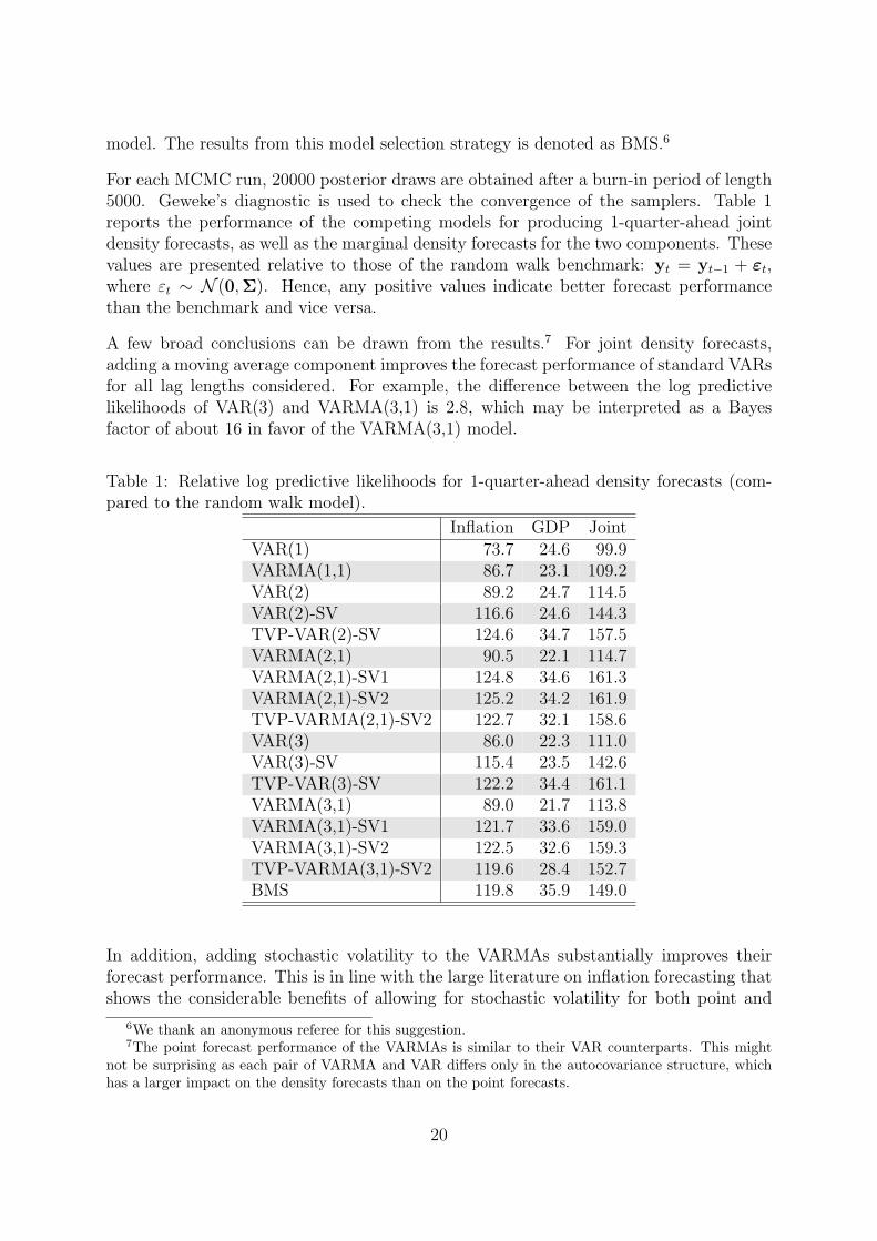
For each MCMC run, 20000 posterior draws are obtained after a burn-in period of length5000. Geweke’s diagnostic is used to check the convergence of the samplers. Table 1reports the performance of the competing models for producing 1-quarter-ahead jointdensity forecasts, as well as the marginal density forecasts for the two components. Thesevalues are presented relative to those of the random walk benchmark: yt = yt−1 + εt,where εt ∼ N (0,Σ). Hence, any positive values indicate better forecast performancethan the benchmark and vice versa.

A few broad conclusions can be drawn from the results.7 For joint density forecasts,adding a moving average component improves the forecast performance of standard VARsfor all lag lengths considered. For example, the difference between the log predictivelikelihoods of VAR(3) and VARMA(3,1) is 2.8, which may be interpreted as a Bayesfactor of about 16 in favor of the VARMA(3,1) model.

Table 1: Relative log predictive likelihoods for 1-quarter-ahead density forecasts (com-pared to the random walk model).

Inflation GDP JointVAR(1) 73.7 24.6 99.9VARMA(1,1) 86.7 23.1 109.2VAR(2) 89.2 24.7 114.5VAR(2)-SV 116.6 24.6 144.3TVP-VAR(2)-SV 124.6 34.7 157.5VARMA(2,1) 90.5 22.1 114.7VARMA(2,1)-SV1 124.8 34.6 161.3VARMA(2,1)-SV2 125.2 34.2 161.9TVP-VARMA(2,1)-SV2 122.7 32.1 158.6VAR(3) 86.0 22.3 111.0VAR(3)-SV 115.4 23.5 142.6TVP-VAR(3)-SV 122.2 34.4 161.1VARMA(3,1) 89.0 21.7 113.8VARMA(3,1)-SV1 121.7 33.6 159.0VARMA(3,1)-SV2 122.5 32.6 159.3TVP-VARMA(3,1)-SV2 119.6 28.4 152.7BMS 119.8 35.9 149.0

In addition, adding stochastic volatility to the VARMAs substantially improves theirforecast performance. This is in line with the large literature on inflation forecasting thatshows the considerable benefits of allowing for stochastic volatility for both point and

6We thank an anonymous referee for this suggestion.7The point forecast performance of the VARMAs is similar to their VAR counterparts. This might

not be surprising as each pair of VARMA and VAR differs only in the autocovariance structure, whichhas a larger impact on the density forecasts than on the point forecasts.

20

density forecasts (see, e.g., Stock and Watson, 2007; Chan, Koop, Leon-Gonzalez, andStrachan, 2012; Clark and Doh, 2014). It is also interesting to note that VARMA(p,1)-SV1and the more general VARMA(p,1)-SV2 perform very similarly, indicating that allowingfor time-variation in Ωt is mostly sufficient. Overall, VARMA(2,1)-SV2 forecasts betterthan all other models.

Consistent with the results in D’Agostino, Gambetti, and Giannone (2013), allowing theVAR coefficients to be time-varying further improves the forecast performance of VAR(p)-SV. Interestingly, this does not hold for VARMAs: adding time-varying VAR coefficientsslightly worsens the forecast performance of VARMA(p,1)-SV2. One possible explanationis that given the VMA coefficients are time-varying, ignoring this time-variation resultsin nonlinearities in the VAR coefficients. By explicitly modeling time-variation in theVMA coefficients, we can keep the VAR coefficients to be constant.

Next, to investigate the source of differences in forecast performance, we look at the logpredictive likelihoods for each series. The results suggest that the gain in adding the mov-ing average and stochastic volatility components comes mainly from forecasting inflationbetter, although adding stochastic volatility also improves forecasting GDP growth tosome extent. Finally, the model selection strategy based on past forecast performance ishighly competitive—it gives the best forecasts for GDP growth. Even when it is not thebest performing model, its performance is comparable to the best.

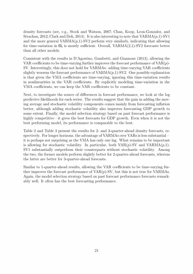
Table 2 and Table 3 present the results for 2- and 3-quarter-ahead density forecasts, re-spectively. For longer horizons, the advantage of VARMAs over VARs is less substantial—it is perhaps not surprising as the VMA has only one lag. What remains to be importantis allowing for stochastic volatility. In particular, both VAR(p)-SV and VARMA(p,1)-SV1 substantially outperform their counterparts without stochastic volatility. Amongthe two, the former models perform slightly better for 2-quarter-ahead forecasts, whereasthe latter are better for 3-quarter-ahead forecasts.

Similar to 1-quarter-ahead results, allowing the VAR coefficients to be time-varying fur-ther improves the forecast performance of VAR(p)-SV, but this is not true for VARMAs.Again, the model selection strategy based on past forecast performance forecasts remark-ably well. It often has the best forecasting performance.

21

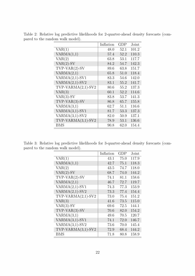
Table 2: Relative log predictive likelihoods for 2-quarter-ahead density forecasts (com-pared to the random walk model).

Inflation GDP JointVAR(1) 48.0 52.1 101.2VARMA(1,1) 57.4 52.2 110.3VAR(2) 63.8 53.1 117.7VAR(2)-SV 84.2 54.7 142.3TVP-VAR(2)-SV 89.6 63.8 151.7VARMA(2,1) 65.8 51.0 118.4VARMA(2,1)-SV1 83.3 54.6 142.0VARMA(2,1)-SV2 83.1 55.2 141.7TVP-VARMA(2,1)-SV2 80.6 55.2 137.3VAR(3) 60.1 52.2 114.6VAR(3)-SV 83.8 53.7 141.3TVP-VAR(3)-SV 86.8 65.7 155.8VARMA(3,1) 62.7 51.1 116.6VARMA(3,1)-SV1 81.7 53.3 137.3VARMA(3,1)-SV2 82.0 50.9 137.1TVP-VARMA(3,1)-SV2 78.9 53.1 136.6BMS 90.8 62.0 154.4

Table 3: Relative log predictive likelihoods for 3-quarter-ahead density forecasts (com-pared to the random walk model).

Inflation GDP JointVAR(1) 43.1 75.0 117.9VARMA(1,1) 42.7 75.1 118.3VAR(2) 43.5 74.7 118.0VAR(2)-SV 68.7 74.0 144.2TVP-VAR(2)-SV 74.1 81.1 158.6VARMA(2,1) 46.7 72.7 119.7VARMA(2,1)-SV1 74.3 77.3 153.9VARMA(2,1)-SV2 73.3 77.4 154.4TVP-VARMA(2,1)-SV2 73.0 75.4 151.2VAR(3) 41.6 73.5 115.0VAR(3)-SV 69.6 72.5 144.1TVP-VAR(3)-SV 70.6 82.0 154.2VARMA(3,1) 49.6 70.5 120.7VARMA(3,1)-SV1 74.1 72.0 146.7VARMA(3,1)-SV2 73.6 70.0 145.4TVP-VARMA(3,1)-SV2 72.9 68.4 144.2BMS 71.8 80.8 158.9

22

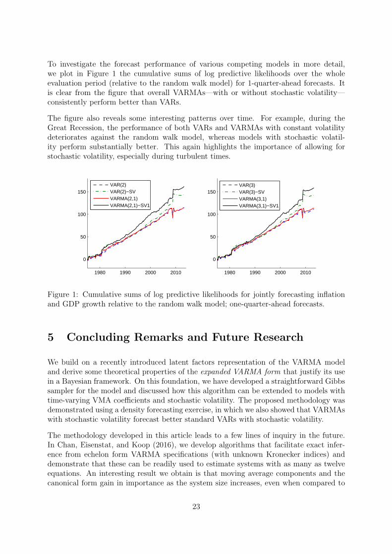
To investigate the forecast performance of various competing models in more detail,we plot in Figure 1 the cumulative sums of log predictive likelihoods over the wholeevaluation period (relative to the random walk model) for 1-quarter-ahead forecasts. Itis clear from the figure that overall VARMAs—with or without stochastic volatility—consistently perform better than VARs.

The figure also reveals some interesting patterns over time. For example, during theGreat Recession, the performance of both VARs and VARMAs with constant volatilitydeteriorates against the random walk model, whereas models with stochastic volatil-ity perform substantially better. This again highlights the importance of allowing forstochastic volatility, especially during turbulent times.

1980 1990 2000 2010

0

50

100

150

1980 1990 2000 2010

0

50

100

150

VAR(2)VAR(2)−SVVARMA(2,1)VARMA(2,1)−SV1

VAR(3)VAR(3)−SVVARMA(3,1)VARMA(3,1)−SV1

Figure 1: Cumulative sums of log predictive likelihoods for jointly forecasting inflationand GDP growth relative to the random walk model; one-quarter-ahead forecasts.

5 Concluding Remarks and Future Research

We build on a recently introduced latent factors representation of the VARMA modeland derive some theoretical properties of the expanded VARMA form that justify its usein a Bayesian framework. On this foundation, we have developed a straightforward Gibbssampler for the model and discussed how this algorithm can be extended to models withtime-varying VMA coefficients and stochastic volatility. The proposed methodology wasdemonstrated using a density forecasting exercise, in which we also showed that VARMAswith stochastic volatility forecast better standard VARs with stochastic volatility.

The methodology developed in this article leads to a few lines of inquiry in the future.In Chan, Eisenstat, and Koop (2016), we develop algorithms that facilitate exact infer-ence from echelon form VARMA specifications (with unknown Kronecker indices) anddemonstrate that these can be readily used to estimate systems with as many as twelveequations. An interesting result we obtain is that moving average components and thecanonical form gain in importance as the system size increases, even when compared to

23

parsimonious Bayesian VARs with shrinkage priors. However, in that work we do notconsider extensions such as stochastic volatility, and this would be one point of interestfor further research.

In addition, empirical investigation of alternative flexible specifications such as regime-switching VARMAs also seems beneficial. Moreover, it is worthwhile to further explorethe relationship of the expanded form to dynamic factor models discussed in Section2. Specifically, it can be shown that reducing the number of “factors” in this VARMArepresentation together with a particular set of restriction on the model parameters leadsto exactly the FAVAR specification. It would therefore be of interest to further investigatehow this relates to the recent work of Dufour and Stevanovic (2013), as well as howalternative identification restrictions compare to the standard ones used in the literature.Lastly, we have focused on forecasting in this paper. Since flexible VARs are now routinelyused for structural analysis, an interesting line of research is to perform similar analysisusing VARMAs with time-varying parameters and stochastic volatility. We leave this forfurther research.

24

References

S. An and F. Schorfheide. Bayesian analysis of DSGE models. Econometric Reviews, 26(2-4):113–172, 2007.

G. Athanasopoulos and F. Vahid. VARMA versus VAR for macroeconomic forecasting.Journal of Business and Economic Statistics, 26(2):237–252, 2008.

G. Athanasopoulos, D. S. Poskitt, and F. Vahid. Two canonical VARMA forms: Scalarcomponent models vis-a-vis the echelon form. Econometric Reviews, 31(1):60–83, 2012.

M. Banbura, D. Giannone, and L. Reichlin. Large Bayesian vector auto regressions.Journal of Applied Econometrics, 25(1):71–92, 2010.

M. A. G. Belmonte, G. Koop, and D. Korobilis. Hierarchical shrinkage in time-varyingparameter models. Journal of Forecasting, 33(1):80–94, 2014.

B. Bernanke, J. Boivin, and P. S. Eliasz. Measuring the effects of monetary policy: Afactor-augmented vector autoregressive (FAVAR) approach. The Quarterly Journal ofEconomics, 120(1):387–422, 2005.

F. Canova. Modelling and forecasting exchange rates with a Bayesian time-varying coef-ficient model. Journal of Economic Dynamics and Control, 17:233–261, 1993.

F. Canova. Methods for Applied Macroeconomic Research. Princeton University Press,New Jersey, 2007.

J. C. C. Chan. Moving average stochastic volatility models with application to inflationforecast. Journal of Econometrics, 176(2):162–172, 2013.

J. C. C. Chan and I. Jeliazkov. Efficient simulation and integrated likelihood estimationin state space models. International Journal of Mathematical Modelling and NumericalOptimisation, 1:101–120, 2009.

J. C. C. Chan, G. Koop, R. Leon-Gonzalez, and R. Strachan. Time varying dimensionmodels. Journal of Business and Economic Statistics, 30:358–367, 2012.

J. C. C. Chan, E. Eisenstat, and G. Koop. Large Bayesian VARMAs. Journal of Econo-metrics, 192(2):374–390, 2016.

T. E. Clark. Real-time density forecasts from Bayesian vector autoregressions withstochastic volatility. Journal of Business and Economic Statistics, 29(3):327–341, 2011.

T. E. Clark and T. Doh. A Bayesian evaluation of alternative models of trend inflation.International Journal of Forecasting, 30(3):426–448, 2014.

T. Cogley and T. J. Sargent. Drifts and volatilities: monetary policies and outcomes inthe post WWII US. Review of Economic Dynamics, 8(2):262 – 302, 2005.

25

T. F. Cooley and M. Dwyer. Business cycle analysis without much theory: A look atstructural VARs. Journal of Econometrics, 83(12):57–88, 1998.

A. D’Agostino, L. Gambetti, and D. Giannone. Macroeconomic forecasting and structuralchange. Journal of Applied Econometrics, 28:82–101, 2013.

M. Del Negro and G. E. Primiceri. Time varying structural vector autoregressions andmonetary policy: A corrigendum. The Review of Economic Studies, 2015. Forthcoming.

T. Doan, R. Litterman, and C. Sims. Forecasting and conditional projection using realisticprior distributions. Econometric reviews, 3(1):1–100, 1984.

J.-M. Dufour and D. Pelletier. Practical methods for modelling weak VARMA processes:identification, estimation and specification with a macroeconomic application. Discus-sion Paper, McGill University, 2014.

J.-M. Dufour and D. Stevanovic. Factor-augmented VARMA models with macroeconomicapplications. Journal of Business & Economic Statistics, 31(4):491–506, 2013.

J. Durbin and S. J. Koopman. A simple and efficient simulation smoother for state spacetime series analysis. Biometrika, 89:603–615, 2002.

E. Eisenstat, J. C. C. Chan, and R. W. Strachan. Model specification search for time-varying parameter VARs. Econometric Reviews, 35(8-10):1638–1665, 2016.

J. C. Engwerda, A. C. M. Ran, and A. L. Rijkeboer. Necessary and sufficient conditionsfor the existence of a positive definite solution of the matrix equationX+A∗X−1A = Q.Linear Algebra and its Applications, 186:255–275, 1993.

J. Fernandez-Villaverde, J. F. Rubio-Ramırez, T. J. Sargent, and M. W. Watson. ABCs(and Ds) of understanding VARs. American Economic Review, 97(3):1021–1026, 2007.

S. Fisk. A note on Weyl’s inequality. The American Mathematical Monthly, 104(3):257–258, 1997.

S. Fruhwirth-Schnatter and H. Wagner. Stochastic model specification search for Gaussianand partial non-Gaussian state space models. Journal of Econometrics, 154:85–100,2010.

E. I. George and R. E. McCulloch. Variable selection via Gibbs sampling. Journal of theAmerican Statistical Association, 88(423):881–889, 1993.

J. Geweke and G. Amisano. Hierarchical Markov normal mixture models with applicationsto financial asset returns. Journal of Applied Econometrics, 26:1–29, 2011.

J. Ghosh and D. B. Dunson. Default prior distributions and efficient posterior compu-tation in Bayesian factor analysis. Journal of Computational and Graphical Statistics,18(2):306–320, 2009.

26

P. Gustafson. On model expansion, model contraction, identifiability and prior informa-tion: Two illustrative scenarios involving mismeasured variables. Statistical Science,20(2):111–140, 2005.

J. D. Hamilton and G. Lin. Stock market volatility and the business cycle. Journal ofApplied Econometrics, 11:573–593, 1996.

E. J. Hannan. The identification and parameterization of ARMAX and state space forms.Econometrica, 44(4):713–723, 1976.

N. J. Higham and H.-M. Kim. Numerical analysis of a quadratic matrix equation. IMAJournal of Numerical Analysis, 20:499–519, 2002.

K. Imai and D. A. van Dyk. A Bayesian analysis of the multinomial probit model usingmarginal data augmentation. Journal of Econometrics, 124(2):311–334, 2005.

C. Kascha. A comparison of estimation methods for vector autoregressive moving-averagemodels. Econometric Reviews, 31(3):297–324, 2012.

C. Kascha and C. Trenkler. Simple identification and specification of cointegratedVARMA models. Journal of Applied Econometrics, 2014. Forthcoming.

S. Kim, N. Shepherd, and S. Chib. Stochastic volatility: Likelihood inference and com-parison with ARCH models. Review of Economic Studies, 65(3):361–393, 1998.

G. Koop. Forecasting with medium and large Bayesian VARs. Journal of Applied Econo-metrics, 2011. DOI: 10.1002/jae.1270.

G. Koop and D. Korobilis. Bayesian multivariate time series methods for empiricalmacroeconomics. Foundations and Trends in Econometrics, 3(4):267–358, 2010.

G. Koop and D. Korobilis. Large time-varying parameter VARs. Journal of Econometrics,177(2):185–198, 2013.

G. Koop and S. M. Potter. Estimation and forecasting in models with multiple breaks.Review of Economic Studies, 74:763–789, 2007.

G. Koop, R. Leon-Gonzalez, and R. W. Strachan. Efficient posterior simulation forcointegrated models with priors on the cointegration space. Econometric Reviews, 29(2):224–242, 2010.

G. Koop, R. Leon-Gonzalez, and R. W. Strachan. Bayesian model averaging in theinstrumental variable regression model. Journal of Econometrics, 171(2):237 – 250,2012.

D. Korobilis. Assessing the transmission of monetary policy shocks using time-varyingparameter dynamic factor models. Oxford Bulletin of Economics and Statistics, 2012.Forthcoming.

27

D. Korobilis. VAR forecasting using Bayesian variable selection. Journal of AppliedEconometrics, 28(2):204–230, 2013.

D. Korobilis. Data-based priors for vector autoregressions with drifting coefficients. Avail-able at SSRN 2392028, 2014.

D. P. Kroese and J. C. C. Chan. Statistical Modeling and Computation. Springer, NewYork, 2014.

D. P. Kroese, T. Taimre, and Z. I. Botev. Handbook of Monte Carlo Methods. John Wiley& Sons, New York, 2011.

E. M. Leeper, T. B. Walker, and S.-C. S. Yang. Fiscal foresight: Analytics and econo-metrics. NBER Working Paper 14028, 2008.

H. Li and R. S. Tsay. A unified approach to identifying multivariate time series models.Journal of the American Statistical Association, 93(442):770–782, 1998.

M. Lippi and L. Reichlin. VAR analysis, nonfundamental representations, blaschke ma-trices. Journal of Econometrics, 63(1):307–325, 1994.

R. Litterman. Forecasting with Bayesian vector autoregressions — five years of experi-ence. Journal of Business and Economic Statistics, 4:25–38, 1986.

J. S. Liu and Y. N. Wu. Parameter expansion for data augmentation. Journal of theAmerican Statistical Association, 94(448):1264–1274, 1999.

H. Lutkepohl. New Introduction to Multiple Time Series Analysis. Springer-Verlag,Berlin, 2005.

H. Lutkepohl and H. Claessen. Analysis of cointegrated VARMA processes. Journal ofEconometrics, 80:223–239, 1997.

H. Lutkepohl and D. S. Poskitt. Specification of echelon-form VARMA models. Journalof Business & Economic Statistics, 14(1):69–79, 1996.

X.-L. Meng and D.A. van Dyk. Seeking efficient data augmentation schemes via condi-tional and marginal augmentation. Biometrika, 86(2):301–320, 1999.

K. Metaxoglou and A. Smith. Maximum likelihood estimation of VARMA models usinga state-space EM algorithm. Journal of Time Series Analysis, 28(5):666–685, 2007.

R. Paap and H. van Dijk. Bayes estimates of Markov trends in possibly cointegrated series:An application to us consumption and income. Journal of Business and EconomicStatistics, 21:547–563, 2003.

M. S. Peiris. On the study of some functions of multivariate ARMA processes. Journalof Time Series Analysis, 25(1):146–151, 1988.

28

D. J. Poirier. Intermediate Statistics and Econometrics: A Comparative Approach. MITPress, Cambridge, 1995.

D. Poskitt and W. Yao. VAR modeling and business cycle analysis: A taxonomy of errors.Journal of Business & Economic Statistics, 2016.

D. S. Poskitt. Vector autoregressive moving average identification for macroeconomicmodeling: A new methodology. Journal of Econometrics, 192(2):468–484, 2016.

G. E. Primiceri. Time varying structural vector autoregressions and monetary policy.Review of Economic Studies, 72(3):821–852, 2005.

N.i Ravishanker and B. K. Ray. Bayesian analysis of vector ARMA models using Gibbssampling. Journal of Forecasting, 16(3):177–194, 1997.

C. A. Sims. Macroeconomics and reality. Econometrica, 48:1–48, 1980.

J. H. Stock and M. W. Watson. Why has U.S. inflation become harder to forecast?Journal of Money Credit and Banking, 39:3–33, 2007.

S.-C. S. Yang. Quantifying tax effects under policy foresight. Journal of MonetaryEconomics, 52(8):1557 – 1568, 2005.

29

A Online Appendix

A.1 Solving the Matrix Quadratic Equation

Following Higham and Kim (2002), solutions to (12) are straightforward to obtain usinggeneralized Schur decompositions. Specifically, define the 2n× 2n matrices

F =

(0 In

−Γ′

1 Γ0

), G =

(In 0

0 Γ1

),

and compute the decomposition F = QSZ∗,G = QTZ∗, whereQ and Z are orthonormal,S and T are upper-triangular, and ∗ denotes the conjugate transpose.8 Next partition

Q =

(Q11 Q12

Q21 Q22

), Z =

(Z11 Z12

Z21 Z22

), S =

(S11 S12

0 S22

)T =

(T11 T12

0 T22

).

Theorem 3 in Higham and Kim (2002) states that every solution to (12) has the form

Θ′

1 = Z21Z−1

11 = Q11S11T−1

11 Q−1

11 . (21)

An important feature of the generalized Schur decomposition is that δi = si/ti (where siand ti are the i-th diagonal elements of S and T, respectively) is a generalized eigenvalue

of the pair (F,G), and if 1 ≤ i ≤ n, it is also an eigenvalue of Θ1. Since

det (F− δG) = det(δ2Γ1 − δΓ0 + Γ

′

1

)= δ2 det

((1

δ

)2

Γ1 −1

δΓ0 + Γ

′

1

), (22)

all generalized eigenvalues come in pairs (δ, 1/δ), including the pairs (0,∞). Therefore,there will be exactly n generalized eigenvalues |δi| < 1 and exactly n generalized eigen-values |δi| > 1.

Note that we are free to rotate the rows and columns of Q, Z, S, T in forming thesolution for Θ1, and so we may choose any rotation that retains a desired subset of ngeneralized eigenvalues of (F,G) to be the eigenvalues of Θ1. For example, to obtainthe fundamental representation, we would choose the rotation that yields S11T

−1

11 withall diagonal elements |si/ti| < 1.

A.2 Proofs of Theorems

Proof of Theorem 1. Let ut = Θ(L)εt be a VMA(q) process with ε being weak whitenoise and no roots of detΘ(L) lying on the unit circle. Then ut is a purely non-deterministic process in a Hilbert space spanned by εt, εt−1, . . . , i.e., ut ∈ L2(ε; t), andεt, εt−1, . . . is a purely non-deterministic process, i.e., limt→−∞ L2(ε; t) = 0.

8Many modern statistical packages have built-in functions for computing generalized Schurdecompositions—in our empirical work, we use the command qz in Matlab.

30

We decompose L2(ε; t) by an orthogonal projection such that L2(ε; t) = L2(ν; t)⊕

L2(ζ; t),and for every ut ∈ L2(ε; t) we can write

ut = Υ(L)νt +Ξ(L)ζt, (23)

where νt and ζt are n × 1, E(νt) = E(ζt) = 0, E(νtν′t) = E(ζtζ

′t) = In, E(νtν

′t−s) =

E(ζtζ′t−s) = 0 for all s ≥ 1, and E(νtζ

′t−s) = 0 for all s ≥ 0. Υ(L) and Ξ(L) are

some finite-order n × n polynomial matrices in the lag operator satisfying rankΥ(L) +rankΞ(L) > n. The latter follows from the fact that any univariate MA with no roots onthe unit circle can be obviously decomposed this way, and any n× n polynomial matrixΘ(L) can be written as the product E(L)Θ†(L), where E(L) is a product of elementarymatrices such that det E(L) is constant (i.e., E(L) is unimodular) and Θ†(L) is upper-triangular.

Without loss of generality, assume Ξ0 ≡ Ξ(0) is invertible. In particular, if neither Ξ0

nor Υ0 are invertible, we can always construct a 2n × 2n Blaschke matrix C(L) (withC(L−1)′C(L) = I2n) such that

(νt

ζt

)=

(C11(L) C12(L)C21(L) C22(L)

)(νtζt

),

Υ(L) = Υ(L)C11(L−1)′ +Ξ(L)C12(L

−1)′,

Ξ(L) = Υ(L)C21(L−1)′ +Ξ(L)C22(L

−1)′,

yields an equivalent representation

ut = Υ(L)νt + Ξ(L)ζt, (24)

but with Ξ0 ≡ Ξ(0) invertible (and Υ(L) 6= 0).9

Proceeding under the assumption that Ξ0 is invertible, further decompose Ξ0ζt = Kξt+ηt, where ξt and ηt are n×1, E(ξt) = E(ηt) = 0, E(ξtξ

′t) = In, E(ηtη

′t) = Λ, E(ξtξ

′t−s) =

E(ηtη′t−s) = 0 for all s ≥ 1, and E(ξtη

′t−s) = 0 for all s ≥ 0. Λ is diagonal with elements

λ2i > 0.

Let ut =∑qν

j=0Υjνt−j +

∑qζj=1Ξjζt−j +Kξt, such that ut = ut + ηt. Observe that ut

is a purely non-deterministic, stationary process with the properties E(utu′t−s) = 0 for

all s > maxqν , qζ and E(utη′t−s) = 0 for all s ≥ 0. Therefore, employing the Wold

decomposition yields

ut =

q∑

j=0

Πjgt, (25)

where gt is n× 1, E(gt) = 0, E(gtg′t) = Ψ, E(gtg

′t−s) = 0 for all s ≥ 1 and E(gtηt−s) = 0

for all s ≥ 0. Π0 = In and Ψ is positive semi-definite (p.s.d.).

9Recall that applying a Blaschke transformation to any orthonormal white noise vector wt, via thetransformation wt = C(L)wt, results in an orthonormal white nose vector wt (see Lippi and Reichlin,1994, for further details).

31

Take the LDU decomposition of Ψ = Φ0ΩΦ′0 and set Φj = ΠjΦ0 for j = 0, . . . , q,

ft = Φ−1

0 gt. SinceE(utu

′t−s) = E((ut + ηt)(ut−s + ηt−s)

′)

for all s ≥ 0 is a necessary condition, it must be that q = q and we obtain the represen-tation (4), which satisfies (6).

Proof of Theorem 2. Similar to the VMA(1) representation (2) of a VMA(q), define thecompanion representation of the expanded form by

utut−1

...ut−q+1

︸ ︷︷ ︸uτ

=

Φ0 Φ1 · · · Φq−1

. . . . . ....

. . . Φ1

Φ0

︸ ︷︷ ︸Φ0

ftft−1

...ft−q+1

︸ ︷︷ ︸fτ

+

Φq

Φq−1

. . ....

. . . . . .

Φ1 · · · Φq−1 Φq

︸ ︷︷ ︸Φ1

ft−qft−q−1

...ft−2q+1

︸ ︷︷ ︸fτ−1

+

ηtηt−1

...ηt−q+1

︸ ︷︷ ︸ητ

(26)

with (fτητ

)∼ WN

((00

),

(Iq ⊗Ω 0

0 Iq ⊗Λ

)). (27)

Accordingly, the mapping in (6) can be written as:

Θ0(Iq ⊗Σ)Θ′

0 + Θ1(Iq ⊗Σ)Θ′

1 = Φ0(Iq ⊗Ω)Φ′

0 + Φ1(Iq ⊗Ω)Φ′

1 + Λ, (28)

Θ1(Iq ⊗Σ)Θ′

0 = Φ1(Iq ⊗Ω)Φ′

0. (29)

Let Ψ = Φ0(Iq ⊗Ω)Φ′

0. Then,

Φ0ΩΦ′0 =

(0 · · · 0 In

)Ψ

0...0

In

, (30)

Φq

...Φ1

= Θ1(Iq ⊗Σ)Θ

′

0Ψ−1

Φ−1

0

0...0

. (31)

Since Φ0 and Ω are obtained uniquely from (30) via the LDU decomposition, we seethat there is a unique mapping from Ψ to Φ0, . . . ,Φq,Ω. In other words, all information

32

about Φ0, . . . ,Φq,Ω is contained in Ψ, so it suffices to analyze the mapping betweenΘ0, . . . ,Θq,Σ and Ψ,Λ.

To this end, substituting (29) into (28) leads to

Γ1Ψ−1Γ

′

1 +Ψ = Γ0 − Iq ⊗Λ, (32)

where Γ0, Γ1 are computed from Θ0, Θ1,Σ as in (3). By definition of P, the set ofpermissible expanded form parameters can be cast as all real positive definite Ψ and Λ

that solve (32). More specifically, Mλ corresponds to the set of all real positive definitesolutions Ψ for a given λ, and L is the set of all λ for which a positive definite solutionΨ to (32) exists.

Engwerda, Ran, and Rijkeboer (1993) demonstrate that a necessary condition for the

existence of a positive definite solution is Γ0 + ρΓ1 + ρ−1Γ′

1 − Iq ⊗ Λ must be positivesemi-definite for all |ρ| = 1, which is equivalent to requiring Hρ − Iq ⊗ Λ to be p.s.d.for all |ρ| = 1. Part 1 of the theorem then follows directly from applying Theorem 1 ofFisk (1997) to the sum −Hρ+ Iq ⊗Λ. Moreover, Proposition 8.2 of Engwerda, Ran, andRijkeboer (1993) states that whenever a solution exists, there are at most a finite numberof real-valued Ψ that solve (32), which proves part 2 of the theorem. Finally, part 1 andpart 2 together imply that the set P is bounded.

To prove the corollary, note that if z∗ is a root of Θ(z) on the unit circle, then z∗ and z∗

are eigenvalues of Θ1Θ−1

0 . Hence, for ρ = −z∗, the matrix Hρ is singular, and there existsa qn×1 vector π—e.g., the eigenvector of Hρ associated with the 0 eigenvalue—such thatπ′Hρπ = 0 and the necessary condition for the existence of a positive definite solutionto (32) reduces to

−π′(Iq ⊗Λ)π ≥ 0,

which has the form

∑

i=1

λ2i

q∑

j=1

π2

i,j = 0,

where πi,j is an element of π. Since at least one πi,j 6= 0, there must be at least oneλ2i = 0. If π does not contain any 0 elements, then λ2i = 0 for all i = 1, . . . , n.

A.3 Details of Sampling Algorithm

In this appendix we discuss the details of Step 2 to Step 4 in the Gibbs sampler forthe VARMA(p, q) model with time-varying parameters and stochastic volatilities in theexpanded form given by (17).

To sample (φ |y,β, f ,h,ψ2

φ,ψ2

h,Λ) in Step 2, note that the innovation ηt has a diagonalcovariance matrix Λ. Hence, we can estimate Φ0,t, . . . ,Φq,t equation by equation. To

33

that end, define y∗t = yt−µ−A1yt−1−· · ·−Apyt−p, and let y∗i,t denote the i-th element

of y∗t .

As discussed in Section 2, we need to impose linear restrictions on the elements ofΦ0,t—inparticular Φ0,t is a lower triangular matrix with ones on the main diagonal—and it willoften be of interest to further impose exclusion restrictions on A1, . . . ,Ap (alternatively,B0, . . . ,Bp for the echelon form) and Φ1,t, . . . ,Φq,t as well. To economize on space, weexplicitly discuss implementing such restrictions on Φ0,t, . . . ,Φq,t; sampling A1, . . . ,Ap

subject to similar restrictions follows analogously. Let φ⋆j,t,i denote the i-th row of Φj,t

and let φj,t,i be the free elements in φ⋆j,t,i, such that

φ⋆0,t,i = R0,iφ0,t,i + ιi,

φ⋆j,t,i = Rj,iφj,t,i, for j > 1,

where ιi is an n × 1 vector with the i-th element ιii = 1 and all others set to zero.Rj,i in this context is a pre-determined selection matrix of appropriate dimensions. Forexample, our assumption that Φ0,t is a lower triangular matrix with ones on the maindiagonal corresponds to R0,i = (Ii−1,0)

′ for i > 1. For i = 1, φ0,1 = ι1 and thereare no free elements. If there are no restrictions imposed on Φ1,t, . . . ,Φq,t, then R1,i =· · · = Rq,i = Inq. Using this formulation, define Ri = diag(R0,1,R1,1, . . . ,Rq,i) andφi,t = (φ′

0,t,i,φ′1,t,i . . . ,φ

′q,t,i)

′, such that

φ⋆i,t = Riφi,t +

(ιi0

)

forms the i-th row of (Φ0,Φ1, . . . ,Φq).

Then, the i-th equation in (17) can be written as

y∗i,t = fi,t + wtRiφi,t + ηi,t, (33)

where wt = (f ′t, f′t−1, . . . , f

′t−q), fi,t is the i-th element of ft, and ηi,t is the i-th element of

ηt. Hence, (18) and (33) define a linear Gaussian state space model for φi,t, and standardalgorithms can be applied. Here we use the algorithm in Chan and Jeliazkov (2009) tojointly sample φi,1, . . . ,φi,T .

To implement Step 3, one can directly apply the algorithm in Del Negro and Primiceri(2015) that is based on the auxiliary mixture sampler of Kim, Shepherd, and Chib (1998)to draw the log-volatilities.

Lastly, Step 4 involves drawing from p(Λ |y,β, f ,φ), p(ψ2

h |h) and p(ψ2

φ |φ). The firstdensity is a product of inverse-gamma densities, and can therefore be sampled from usingstandard methods:

(λ2i |y,β, f ,φ) ∼ IG

(νλ,0 + T/2, Sλ,0 +

T∑

t=1

(y∗i,t − fi,t − wtRiφi,t)2/2

).

The last two densities are nonstandard, but we can sample from them using a Metropolis-Hastings step with a tailored proposal density. For example, to sample ψ2

h,i, we first obtain

34

a candidate draw ψ2∗h,i from the proposal IG((T − 3)/2,

∑T

t=2(hi,t− hi,t−1)

2/2). Given thecurrent draw ψ2

h,i, the candidate ψ2∗h,i is accepted with probability

min

1,

(ψ2∗h,i)

− 1

2 e− 1

2Sh,0ψ2∗

h,i

(ψ2h,i)

− 1

2 e− 1

2Sh,0ψ2

h,i

;

otherwise we keep the current draw ψ2h,i. We sample ψ2

φ,i,j similarly.

35