eﬃcient characteristic hulls - geosensor.net

DR

AFT

Efficient characteristic hulls

Matt Duckham1, Lars Kulik2, Mike Worboys3, Antony Galton4

1. Department of GeomaticsUniversity of Melbourne, Victoria, 3010, Australia

[email protected]

2. Department of Computer Science and Software EngineeringUniversity of Melbourne, Victoria, 3010, Australia

[email protected]

3. National Center for Geographic Information and AnalysisUniversity of Maine, Orono, ME 04469, USA

[email protected]

4. Department of Computer ScienceUniversity of Exeter, Exeter EX4 4QF, UK

[email protected]

Abstract. This paper presents a simple, flexible, and efficient algorithmfor constructing a possibly non-convex polygon that characterizes theshape of a set of input points in the plane, termed a characteristic hull.The algorithm is based on the Delaunay triangulation of the points. Theshape produced by the algorithm is controlled by a single normalizedparameter, which can be used to generate a finite, totally ordered familyof related characteristic hulls, varying between the convex hull at oneextreme and a uniquely defined shape with minimum area. These char-acteristic hulls possess a number of desirable properties, including someproperties closely related to pseudohulls. The paper includes an empiricalinvestigation of the shapes produced by the algorithm. This investigationprovides experimental evidence that with appropriate parameterizationthe algorithm is able to accurately characterize the shape of a wide rangeof different point distributions and densities. The experiments detail theeffects of changing parameter values and provide an indication of some“good” parameter values to use in certain circumstances.

1 Introduction

The construction of convex hulls is a fundamental operation in computationalgeometry. In the Cartesian plane, the convex hull of a set of points S is thesmallest convex polygon which contains all points in S. However, for sets ofpoints with a pronounced non-convex distribution the convex hull can neverprovide good characterization of that distribution.

DR

AFT

2 Duckham, Kulik, Worboys, and Galton

In this paper we present an algorithm for building “non-convex hulls.” Thealgorithm is as efficient as an optimal convex hull algorithm, O(n log n) com-putation time for n points. For a finite set of input points P , the algorithmproduces a simple, possibly non-convex polygon that contains all the points inP and is contained within and possibly equal to the convex hull. We refer to thepolygons produced by the algorithm as “characteristic hulls,” and the algorithmitself as the characteristic hull or K (kappa) algorithm.

Two features of our characteristic hulls are worth highlighting at this point.First, while there exists only one convex hull for a set of points there can bemany different characteristic hulls. There is no “correct” characteristic hull. Weargue that in many cases the algorithm yields a better characterization of dis-tribution of a set of points than the convex hull. To illustrate, figure 1 showsa gallery of convex and characteristic hulls for some example point sets withclearly non-convex distributions. However, deciding precisely what constitutes a“better characterization” of the distribution of a set of points is as much a mat-ter for human cognition and preference as for computational geometry. Despitethis inherent underspecification in the problem statement, we argue that thecharacteristic hulls produced by our algorithm are useful. Further, we exploreexperimentally some of the attributes of a shape which may constitute “better”or “worse” characterizations of the distribution of a set of points. We also pro-pose some natural choices for parameterizing our characteristic hull algorithmin a way that generates a uniquely defined result.

Second, characteristic hulls are simple (Jordan) polygons, homeomorphic tothe closed unit disk. Thus, characteristic hulls are simply connected (all of onepiece containing no holes nor islands) and regular. In some cases, however, thedistribution of a set of points may be best characterized by multiple (possiblynon-convex) polygons enclosing disconnected regions of space (e.g., an “i” or“=”shape). In this paper we do not consider directly such cases and are solelyconcerned with cases where the distribution of points can be adequately charac-terized as a single simple polygon. However, we note that it would be possibleto deal with such cases indirectly by first preprocessing the input point set topartition it into subsets, each of which may be adequately characterized by asingle simple polygon. The partitioning of the point sets could be accomplishedusing existing clustering techniques, which are legion, but these possibilities arenot discussed further in this paper. In other cases where the distribution ofpoints is best characterized using a polygon containing one or more holes (e.g.,an “8” shape), the characteristic hull algorithm presented in this paper will notbe able to generate these holes. It will, however, still successfully generate acharacterization of the external edge of such a region.

2 Related work

An early, and influential, attempt to characterize the shape of a set of points isdue to [10], who introduced a construction known as “α-shape” as a generaliza-tion of the convex hull. For a finite set P of points in the plane, the “α-hull” for

DR

AFT

Efficient characteristic hulls 3

The convex hull of P Input point set P A characteristic hull of P

Fig. 1. Gallery of convex hulls and characteristic hulls for several point sets in theplane

DR

AFT


α �= 0 is the intersection of all closed discs of radius 1/α containing all the pointsof P (where for negative values of α a closed disk of radius 1/α is interpreted asthe complement of an open disk of radius −1/α). As α approaches 0, the α-hullapproaches the ordinary convex hull, and therefore the 0-hull is stipulated to bethe convex hull. The α-shape is a straight-line graph (usually a polygon) derivedin a straightforward manner from the α-hull. When α = 0, this is the convexhull, and for large negative values of α it is P itself.

A related notion, A-shape, was introduced by [17]. Given a finite set of pointsP , and a set A (which evidently needs to be disjoint from P , although the authorsdo not specify this), we can define the A-shape of P by first constructing theVoronoi diagram for A∪P and then joining together any pair of points p, q ∈ Pwhose Voronoi cells both border each other and border some common Voronoicell containing a point of A. The edges pq belong to the Delaunay triangulationof A ∪ P : they are the “A-exposed” edges of the triangulation. An importantissue discussed in the paper is how to choose A so that the A-shape of P is“adequate.” In a later paper [12], the A-shape is used as the basis for an “onion-peeling” method, by analogy with the popular convex onion-peeling method fororganizing a set of points and extracting a “central” embedded convex shapefrom them [8].

Two rather different constructs, r-shape and s-shape, were defined by [7] asfollows. The initial set of points P is assumed to be a dot pattern, that is, a planarpoint set whose elements are “clearly visible as well as fairly densely and moreor less evenly distributed.” To obtain the s-shape, the plane is partitioned into alattice of square cells of side-length s. The s-shape is simply the union of latticecells containing points of P . The authors suggest a procedure for optimizing thevalue of s so that the s-shape best approximates the perceived shape of the dotpattern. For the r-shape, they first construct the union of all disks of radius rcentered on points of P . For points p, q ∈ P , the edge pq is selected if and onlyif the boundaries of the disks centered on p and q intersect in a point which lieson the boundary of the union of all the disks. The r-shape of P is the unionof the selected edges, and the authors show that this can be computed in timeO(n), where n is the cardinality of P . They note that the r-shape is a subgraphof the α-shape in the sense of Edelsbrunner. Regarding the selection of r, theynote that “to get a perceptually acceptable shape, a suitable value of r should bechosen, and there is no closed form solution to this problem,” and that moreover“‘perceptual structure’ of P ... will vary from one person to another to a smallextent.”

An alternative method, also designed to be applied to dot patterns, wasproposed by [14]. This procedure starts by constructing the convex hull of thepoints, and then uses a “split and merge” procedure to successively insert extraedges or smooth over zigzags. The splitting procedure results in a highly jaggedoutline, which is then made smoother by the merging procedure. The resultingoutline gives an approximation to the perceived shape of the dot pattern. Thecomplexity of the procedure is limited by the complexity of finding the initialconvex hull, O(n log n).

DR

AFT


The use of Voronoi diagrams for constructing regions from point-sets hasalso been advocated in the context of GIS [1]. In this context, the set P consistsof points known to be in a certain region, for which an approximation to theboundary is required. It is assumed that in addition to P another point-set P ′ isgiven, consisting of points known to lie outside the region to be approximated.From the Voronoi diagram for P ∪ P ′, the method simply selects the union ofthe Voronoi cells containing points of P . The resulting shape differs from thecharacteristic hulls constructed in this paper in that the original point-set liesentirely in its interior. Depending on one’s purposes, this feature may either bedesirable or undesirable.

A similar method [4] is based on Delaunay triangulations. Given sets P andP ′ as before, the Delaunay triangulation of P ∪ P ′ is constructed, and then themidpoint of every edge which joins a point in P to a point in P ′ is selected. Thefinal region is produced by joining all pairs of selected midpoints belonging toedges of the same triangle.

In all these cases, as with the method we describe in this paper, the goal isto generate a region which in some sense “covers” the given set of points, someof which may end up on the boundary of the region, others in its interior. Asomewhat different, though related problem, is to generate a region such thatall of the points lie on its boundary. A typical application, in three dimensions,works with points which are sampled from the surface of some three-dimensionalobject, the intention being to reconstruct the entire surface from the samples.Methods which have been used for this problem include the Power Crust methodof [2, 3], which first generates a finite union of balls as an approximation to themedial axis transform of the object, and then derives from this a piecewise-linearapproximation to the object’s surface—the power crust. The balls chosen are asubset of the Voronoi balls for the set of samples. An alternative approach tothe same problem, based on the Delaunay tessellation rather than the Voronoi,is given by [5].

Given that a considerable amount of research has been done on finding re-gions corresponding to point-sets, and much of this research takes convex hulls,Voronoi diagrams, or Delaunay triangulations as its starting point, it is perhapssurprising that our Delaunay-based method, though extremely simple in con-ception, does not appear to have been proposed before. With so many differentmethods in existence, all giving different results, there is a clear need for somesystematic comparison of the methods and evaluation of their relative merits indifferent application contexts. Some initial work suggesting criteria upon whichto base such a systemic comparison is given in [13]. However, in the remainderof this paper we concentrate primarily on the presentation of our algorithm andits properties.

3 The K (kappa) algorithm

For a finite set of at least three points in the Cartesian plane P ⊂ R2, the

characteristic hull (K—kappa) algorithm yields a possibly non-convex area with

DR

AFT


a shape that “characterizes” the distribution of the input point set. All the setsunder consideration in this paper are sets of points in the Cartesian plane R

2,and in most cases these sets are assumed to be finite, although in those caseswhere infinite sets are discussed this will be made explicit. The characteristichull produced by the algorithm has the properties that:

1. it is a simple polygon;2. it contains all the points of P ; and3. it bounds an area contained within and possibly equal to the convex hull of

the points of P .

The K algorithm is based on “shaving” exterior edges from a triangulationof the input point set in order of the length of edges and subject to a regularityconstraint. The algorithm itself has a time complexity of O(n log n), where n isthe number of input points. Although the algorithm is presented in detail in thefollowing section, it can be summarized as comprising the following steps for aninput point set P and a length parameter l:

1. Generate the Delaunay triangulation of the set of input points P ;2. Remove the longest exterior edge from the triangulation such that:

(a) the edge to be removed is longer than the length parameter l; and(b) the exterior edges of the resulting triangulation form the boundary of a

simple polygon;3. Repeat 2. as long as there are more edges to be removed4. Return the polygon formed by the exterior edges of the triangulation

In exploring the algorithm more carefully, we begin with some preliminarymaterial on the underlying structure for the triangulation, a combinatorial map(3.1). Then we present the algorithm itself (3.2). In the next section (4) we discussthe properties of the algorithm and the non-convex hull, introduced above, inmore detail.

3.1 Combinatorial maps

The K algorithm is based on an explicit orientation of the edges in the tri-angulation around a given vertex. The orientation of edges in a graph can berepresented by oriented combinatorial maps. Introduced in [11], combinatorialmaps are well-known in computational geometry, and are the formal basis ofseveral common data structures, such as the winged-edge and half-edge datastructures [6, 20]. The following definitions build on the functional specificationof combinatorial maps given in [9].

Definition 1. A (2-dimensional) oriented combinatorial map, or just map, M,is a triple 〈D, Θ0, Θ1〉, where D is a finite set of elements, called darts, Θ0 is aninvolutory bijection on D (i.e., Θ2

0 = 1), and Θ1 is a bijection on D. We mayalso assume that Θ0 has no fixed points.

DR

AFT


Θ0 partitions the set of darts into sets of pairs of darts, and each such pair iscalled an edge of map M. Each of the cycles of Θ1 represents a vertex of M. It isstraightforward to use Θ0 and Θ1 to calculate the ordering of edges round facesin a combinatorial map. The cycles of the composition Θ0Θ1 gives the orderingof darts, and converting the darts to their (unique) associated edges gives theordering of edges. In general, a face of map M is a cycle of edges associated witha cycle of darts in Θ0Θ1. Alternatively, focusing on vertices rather than edges,we can consider the cycle of vertices (uniquely) associated with the edges to bethe face.

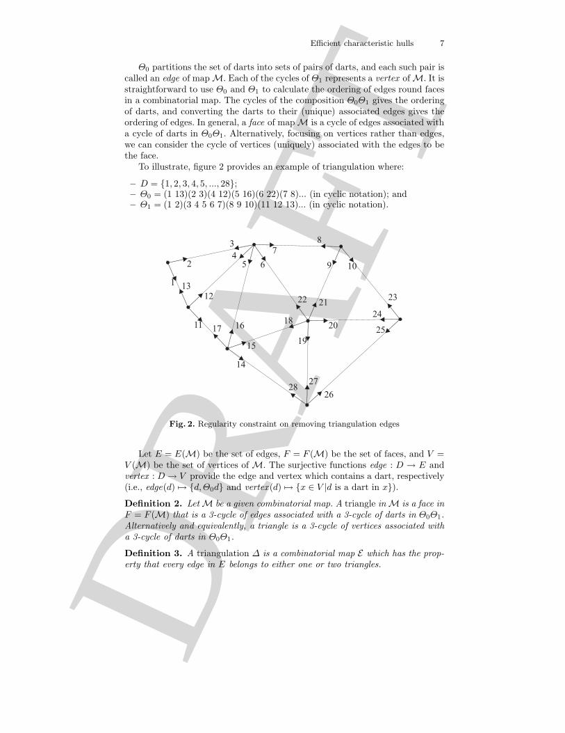
To illustrate, figure 2 provides an example of triangulation where:

– D = {1, 2, 3, 4, 5, ..., 28};– Θ0 = (1 13)(2 3)(4 12)(5 16)(6 22)(7 8)... (in cyclic notation); and– Θ1 = (1 2)(3 4 5 6 7)(8 9 10)(11 12 13)... (in cyclic notation).

4

1

2

37

5

11

109

8

6

1817 16

2322 21

20

19

2827

26

25

24

15

14

1312

Fig. 2. Regularity constraint on removing triangulation edges

Let E = E(M) be the set of edges, F = F (M) be the set of faces, and V =V (M) be the set of vertices of M. The surjective functions edge : D → E andvertex : D → V provide the edge and vertex which contains a dart, respectively(i.e., edge(d) → {d, Θ0d} and vertex (d) → {x ∈ V |d is a dart in x}).Definition 2. Let M be a given combinatorial map. A triangle in M is a face inF = F (M) that is a 3-cycle of edges associated with a 3-cycle of darts in Θ0Θ1.Alternatively and equivalently, a triangle is a 3-cycle of vertices associated witha 3-cycle of darts in Θ0Θ1.

Definition 3. A triangulation Δ is a combinatorial map E which has the prop-erty that every edge in E belongs to either one or two triangles.

DR

AFT


From now on we will work with triangulations rather than more general combi-natorial maps. Suppose from now on that our underlying triangulation is Δ.

Definition 4. An interior edge of Δ is an edge that belongs to two triangles inΔ. A boundary edge of Δ is an edge that belongs to exactly one triangle in Δ.The edge-interior of Δ is the collection of its interior edges. The edge-boundaryof Δ is the collection of its boundary edges.

Definition 5. An interior vertex of Δ is a vertex containing no boundary edges.A boundary vertex of region Δ is a vertex containing boundary edges. Thevertex-interior of Δ is the collection of its interior vertices. The vertex-boundaryof Δ is the collection of its boundary vertices.

Definition 6. A triangle is an interior triangle of Δ if all its edges are interioredges of Δ. A triangle is a boundary triangle of Δ if at least one of its edgesis a boundary edge of Δ. The triangle-interior of Δ is the collection of interiortriangles of Δ. The triangle-boundary of Δ is the collection of its boundarytriangles.

Definition 7. A triangulation Δ is regular if each boundary vertex of Δ con-tains exactly two boundary edges of R.

Definition 8. A planar embedding of Δ is a function f : V (Δ) → R2 from

the set of vertices in Δ to points in the plane. The length of an edge ||e|| is theEuclidean distance δ(a, b) where a = vertex(d), b = vertex (Θ0(d)), and d ∈ e isa dart of e.

3.2 Algorithm

The K algorithm has two components. The main component (Algorithm 1)takes a set of points and a non-negative length parameter l as input. Algorithm1 constructs the Delaunay triangulation of the input point set (line 1.1) and thelist of boundary edges B sorted in descending order of edge length (lines 1.3–1.8).Next, the algorithm cycles through each boundary edge in order (longest first,lines 1.10–1.14). At each iteration the longest boundary edge is removed (line1.11) from B. Additionally, this edge will be removed from the triangulation if:

1. the resulting triangulation is regular; and2. the edge length is at least l (line 1.12).

When an edge e is removed, the two new boundary edges that are revealed bythe removal of e are added to the list of boundary edges B, respecting the edge-length ordering of B (line 1.14). The boundary edges that are revealed by theremoval of an edge can be found using the combinatorial map. For this purposewe define the function reveal : D → D as follows.

reveal(d) →{

Θ1d if Θ0Θ1Θ0Θ1Θ0Θ1d = d

Θ0Θ1Θ0Θ1Θ0d otherwise(1)

DR

AFT


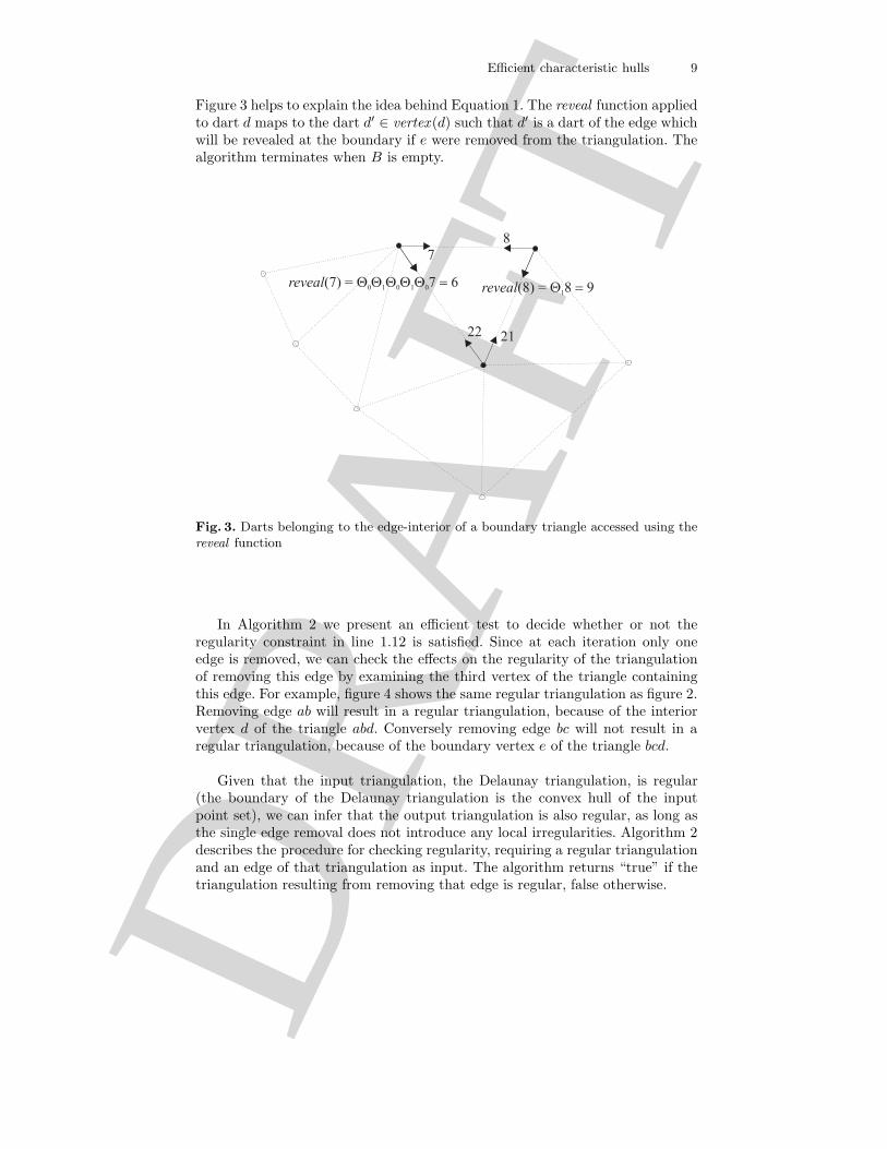
Figure 3 helps to explain the idea behind Equation 1. The reveal function appliedto dart d maps to the dart d′ ∈ vertex(d) such that d′ is a dart of the edge whichwill be revealed at the boundary if e were removed from the triangulation. Thealgorithm terminates when B is empty.

7

8

reveal(7) = � ��

22 21

reveal(8) = ��

Fig. 3. Darts belonging to the edge-interior of a boundary triangle accessed using thereveal function

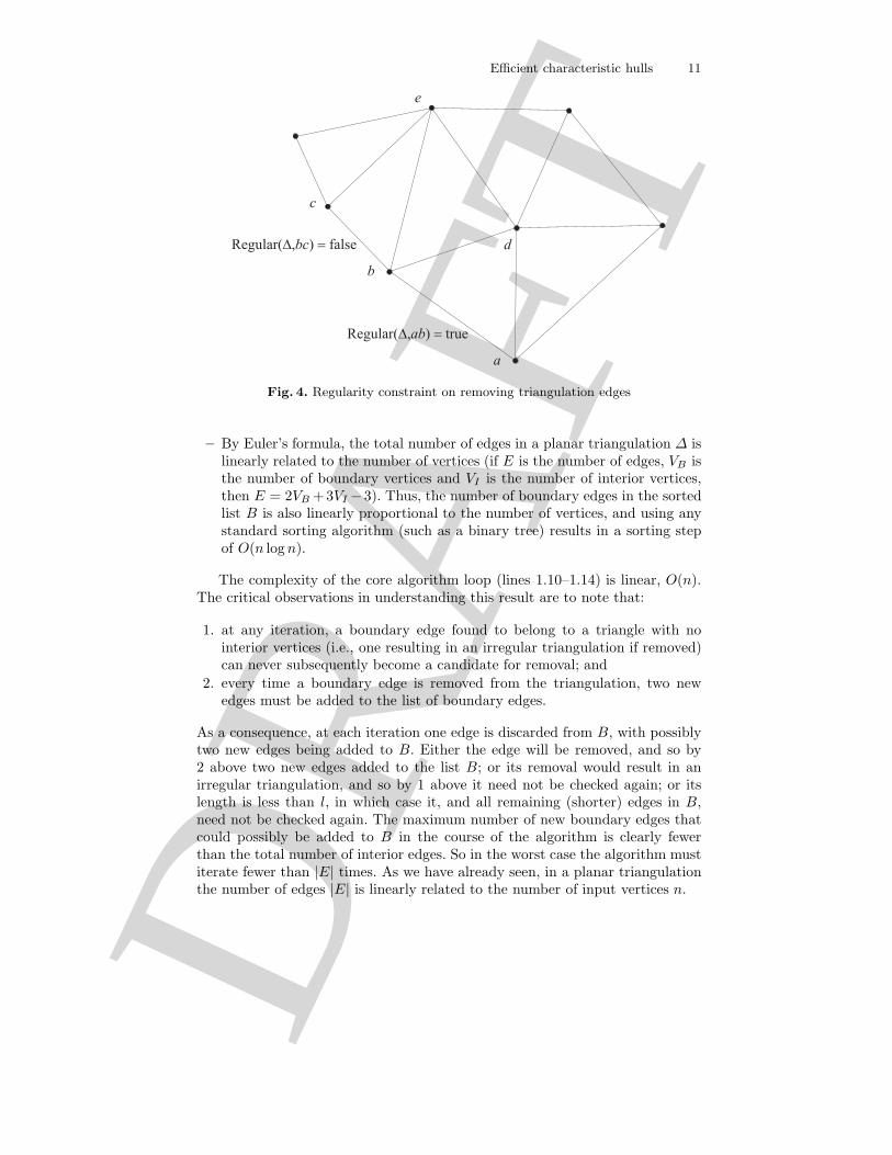
In Algorithm 2 we present an efficient test to decide whether or not theregularity constraint in line 1.12 is satisfied. Since at each iteration only oneedge is removed, we can check the effects on the regularity of the triangulationof removing this edge by examining the third vertex of the triangle containingthis edge. For example, figure 4 shows the same regular triangulation as figure 2.Removing edge ab will result in a regular triangulation, because of the interiorvertex d of the triangle abd. Conversely removing edge bc will not result in aregular triangulation, because of the boundary vertex e of the triangle bcd.

Given that the input triangulation, the Delaunay triangulation, is regular(the boundary of the Delaunay triangulation is the convex hull of the inputpoint set), we can infer that the output triangulation is also regular, as long asthe single edge removal does not introduce any local irregularities. Algorithm 2describes the procedure for checking regularity, requiring a regular triangulationand an edge of that triangulation as input. The algorithm returns “true” if thetriangulation resulting from removing that edge is regular, false otherwise.

DR

AFT


Algorithm 1: Characteristic hull algorithm: K(P, l)Data: Set of points P ⊂ R× R; length l ∈ R

Result: Characteristic hull K(P, l)Construct the Delaunay triangulation Δ of P ;1.1

Construct the list L← [e1, e2, ..., en] containing the set of edges E(Δ);1.2

while L �= ∅ do1.3

Set e← head(L);1.4

Remove e from L;1.5

if e is a boundary edge then1.6

Store e in B, the list of boundary edges;1.7

Sort the list B in descending order of edge length;1.8

while B is not empty do1.9

Set e← head(B);1.10

Remove e from B;1.11

if ||e|| > l and Regular(Δ, e) then1.12

Remove edge e from triangulation Δ;1.13

Insert the two edges edge(reveal (d1)) and edge(reveal (d2)) into B in1.14

order of edge length, where d1 and d2 are the two darts in e;

return the polygon formed by the set of boundary edges of triangulation Δ;1.15

Algorithm 2: Regularity algorithm: Regular(Δ, e)Data: Regular triangulation Δ, edge e of ΔResult: True if Δ− e is regular, false otherwiseif e is a boundary edge of Δ then2.1

Set v to be the (unique) vertex v = vertex (Θ0(reveal (d))) for an arbitrary2.2

dart d ∈ e;if v is an interior vertex of Δ then2.3

return true;2.4

return false;2.5

4 Properties

The properties of the K algorithm and the characteristic hull have been intro-duced at the beginning of section 3. In this section we explore these propertiesin more detail.

4.1 Algorithmic properties

In this section we show that the time complexity of Algorithm 1 is O(n log n),where n is the cardinality of the input point set. The two preprocessing steps(line 1.1 and 1.8) each require O(n log n) time:

– It is a standard result in computational geometry that the Delaunay trian-gulation (line 1.1) can be computed in O(n log n) time (see [18]).

DR

AFT


a

b

c

d

e

Regular( true�� ab

Regular( false�� bc

Fig. 4. Regularity constraint on removing triangulation edges

– By Euler’s formula, the total number of edges in a planar triangulation Δ islinearly related to the number of vertices (if E is the number of edges, VB isthe number of boundary vertices and VI is the number of interior vertices,then E = 2VB +3VI −3). Thus, the number of boundary edges in the sortedlist B is also linearly proportional to the number of vertices, and using anystandard sorting algorithm (such as a binary tree) results in a sorting stepof O(n log n).

The complexity of the core algorithm loop (lines 1.10–1.14) is linear, O(n).The critical observations in understanding this result are to note that:

1. at any iteration, a boundary edge found to belong to a triangle with nointerior vertices (i.e., one resulting in an irregular triangulation if removed)can never subsequently become a candidate for removal; and

2. every time a boundary edge is removed from the triangulation, two newedges must be added to the list of boundary edges.

As a consequence, at each iteration one edge is discarded from B, with possiblytwo new edges being added to B. Either the edge will be removed, and so by2 above two new edges added to the list B; or its removal would result in anirregular triangulation, and so by 1 above it need not be checked again; or itslength is less than l, in which case it, and all remaining (shorter) edges in B,need not be checked again. The maximum number of new boundary edges thatcould possibly be added to B in the course of the algorithm is clearly fewerthan the total number of interior edges. So in the worst case the algorithm mustiterate fewer than |E| times. As we have already seen, in a planar triangulationthe number of edges |E| is linearly related to the number of input vertices n.

DR

AFT


Note also that checking whether removing an edge will result in a regulartriangulation (line 1.12 and Algorithm 2) can be achieved in constant time. Forthe boundary edge in question, it is only necessary to look up whether the thirdvertex of the boundary triangle containing that edge is an interior vertex. Thisthird vertex can be found directly from the combinatorial map. Further notethat checking whether an edge (or equivalently a vertex) is an interior edge

Consequently, the overall time complexity of the K algorithm is dominatedby the preprocessing steps, and is O(n log n).

4.2 Characteristic hull properties

A polygon X is a closed planar path composed of a finite number of sequentialline segments. The straight line segments that make up X are called its edgesand the points where the sides meet are the vertices. Polygon X is said to besimple if the only points of the plane belonging to two polygon edges of X arethe polygon vertices of X . Clearly, so long as the points are not all collinear, theinitial triangulation is regular, and hence yields a hull that is simple (the convexhull). Each iteration of the algorithm preserves regularity. A regular triangulationmust have a simple polygon boundary, by the definition of regularity in section3.1. Thus, the characteristic hull must also be simple.

The initial triangulation contains all the elements of initial point set as ver-tices, thus initially all elements of the point set must be incident with at leasttwo edges. Since the algorithm removes at most one edge from the triangulationat each iteration, an element of the input point set can only lie outside the char-acteristic hull if first at some iteration it was a vertex incident with only oneedge. Such a situation is prohibited by the regularity constraint. Thus, we inferthat the entire input point set must be vertices of the final triangulation, and socontained within the characteristic hull.

Finally, the area bounded by the characteristic hull must be contained withinand possibly equal to the convex hull. In the extreme case where no edges areremoved, then the algorithm returns the polygon boundary of the convex hull.Every iteration of the algorithm that removes an edge from the triangulation willexclude those parts of the convex hull that were contained within the trianglebounded by the deleted edge.

5 Parameterization

The shape of the characteristic hull produced by the algorithm described above isparameterized using the length l. Because the algorithm runs through boundaryedges in descending order, any edge that is removed for a parameter l will alsobe removed for a smaller parameter l′ < l. Thus, for any set of input points Pand length parameters l′ ≤ l, it follows that the characteristic hull of P withparameter l′ is contained within the characteristic hull of P with parameter l,i.e., l′ ≤ l ↔ K(P, l′) ⊆ K(P, l).

DR

AFT


5.1 Normalized length parameters

The parameter l can potentially take the value of any non-negative real number.However, it is more convenient to normalize the parameter with respect to aparticular set of points P by using the maximum and minimum edge lengths ofthe Delaunay triangulation of P . Increasing l beyond the maximum edge lengthof the Delaunay triangulation cannot reduce the number of edges that will beremoved (which will be zero anyway). Decreasing l beyond the minimum edgelength of the Delaunay triangulation cannot increase the number of edges thatwill be removed. Thus, for a set of points P we define two lengths maxP andminP as follows:

maxP ≡ max({||e|| | e ∈ E(ΔP )})

minP ≡ min({||e|| | e ∈ E(ΔP )})Given these two lengths, we can now define a normalized length parameter

λP ∈ [0, 1] as follows:

λP =

⎧⎪⎨⎪⎩

1 if l > maxP

l−minP

maxP −minPif minP ≤ l ≤ maxP

0 if l < minP

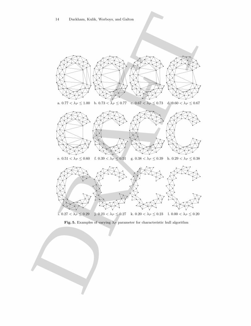
Figure 5 shows an example of all the different characteristic hulls producedby different normalized λP parameters for a sparse set of points P roughly inthe shape of the letter “C”. To help illustrate the effects of the λP parameter,figure 5 shows the full triangulation associated with each λP value. However, itshould be noted that the K algorithm only returns the polygonal boundary forthe triangulation, not the full triangulation itself.

5.2 Choices of λP

As shown above, the choice of λP has a determining effect on the precise shapeobtained from the characteristic hull algorithm. One way of choosing a valuefor λP , then, is to try a range of different values and then a posteriori selectthe value that produces a shape that best fits some desired criteria (such asarea-perimeter ratio). However, there are a range of possible a priori choices forvalues of λP that can be selected in advance of executing the algorithm.

Two natural choices are to set λP to an extreme value, zero or one. Setting λP

to one means that no edges will be removed from the Delaunay triangulation, sothe resulting polygon will be the convex hull (Figure 5.a). While it is useful thatthe K algorithm degrades gracefully to yield the convex hull at one extreme,it is to be expected that in most cases removal of some edges is required tobetter characterize the input set of points. Setting λP to zero means that alledges that can be removed subject to the regularity constraint will be removed(Figure 5.l). However, running the K algorithm to its conclusion in this way

DR

AFT


a. 0.77 < λP ≤ 1.00 b. 0.73 < λP ≤ 0.77 c. 0.67 < λP ≤ 0.73 d. 0.60 < λP ≤ 0.67

e. 0.51 < λP ≤ 0.60 f. 0.39 < λP ≤ 0.51 g. 0.38 < λP ≤ 0.39 h. 0.29 < λP ≤ 0.38

i. 0.27 < λP ≤ 0.29 j. 0.23 < λP ≤ 0.27 k. 0.20 < λP ≤ 0.23 l. 0.00 < λP ≤ 0.20

Fig. 5. Examples of varying λP parameter for characteristic hull algorithm

DR

AFT


often creates polygons that are eroded beyond the point where they provide adesirable characterization of the shape.

Given that extreme values of λP tend to lead to unsatisfactory convex hulls,it would be useful to be able to define a priori an intermediate value for theparameter, 0 < λP < 1, that could adapt to a range of different point sets toproduce acceptable shape characterizations. For example, one possibility investi-gated was to use the length of the longest edge in the minimum spanning tree ofthe Delaunay triangulation (which we coined the “max-MST” edge length). Theminimum spanning tree is the subgraph of the Delaunay triangulation with thesmallest total edge length that connects all the vertices of the triangulation. Inthe case of the point distribution in figure 5, above, the max-MST edge lengthcorresponded to a λP value of 0.1, yielding the shape in figure 5.l. A secondpossibility was to find the shortest edge for each triangle in the Delaunay tri-angulation, and use the maximum length of all these shortest edges (which wetermed the “max-min Δ” edge length). For the point distribution in figure 5, themax-min Δ edge length corresponded to a λP value of 0.56, yielding the shapein figure 5.e.

Initial investigations using these two possibilities revealed that while one orother sometimes provided a satisfactory result, neither could be be relied uponto consistently provide a “good” characterization of shape (as illustrated byFigure ??, where neither parameter yields a shape that closely approximatesthe “C” shape of the original point distribution). Potentially, there are manyother possible a priori choices of λP that might be defined. For example, anintermediate value of λP half-way between the max-MST and max-min Δ valuesoften, but not always, yielded satisfactory results.

As already highlighted in section 1, unlike convex hulls there are many pos-sible characteristic hulls. The criteria for what makes one shape a “better” char-acterization of a set of points than another are underspecified, and are usu-ally connected with a shape’s “visual salience” to a human [13]. Thus, it is tobe expected that the K algorithm provides a range of possible characteristichulls for different λP values. Although definitions like the “maximum MST”and “maximum-minimum triangle” edge lengths provided a principled methodfor a priori choosing an intermediate λP , such methods cannot be expected toconsistently provide a “good” characterization of the shape of a set of points.

5.3 Relationship to axiomatic hull properties

As we have seen, the K algorithm produces a family of results depending on thechoice of length parameter l (alternatively normalized length λP with respect topoint set P ). For a fixed length parameter l, the K algorithm has a number ofimportant properties that relate to the general properties of hulls.

Geometry provides a general definition of a hull. For any set of input pointsS, a hull operator H should have the following axiomatic properties, set outin [15]:

H1 S ⊆ H(S)

DR

AFT


H2 S′ ⊆ S → H(S′) ⊆ H(S) for all S′

H3 H(H(S)) ⊆ H(S)

Axiom H1 stipulates that a hull should contain all its input points. Togetherthe three axioms ential idempotency: H(H(S)) = H(S). In the case of the Kalgorithm, by definition H1 always holds for any length parameter l. In principle,we could hope H3 might also hold. However, the hull definition above is toogeneral for our purposes. The general definition above assumes the input set Scan be infinite, (hence the hull operator can be iterated), while we require afinite set of points as the input to the K algorithm.

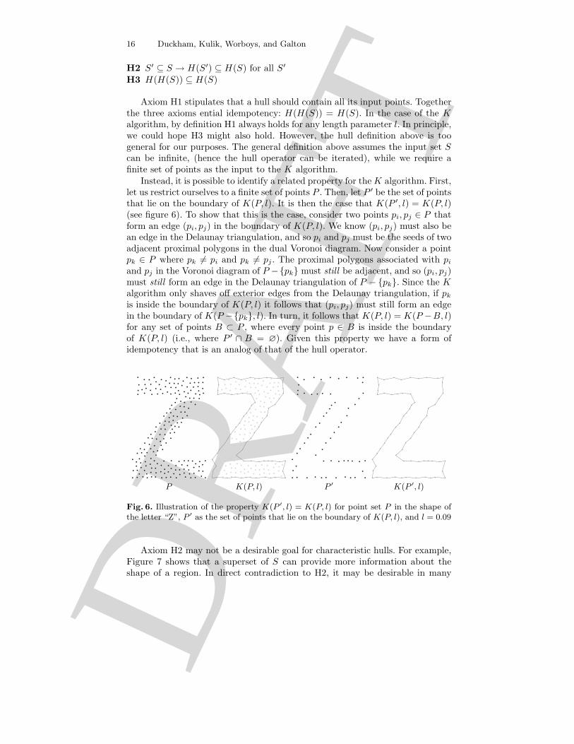
Instead, it is possible to identify a related property for the K algorithm. First,let us restrict ourselves to a finite set of points P . Then, let P ′ be the set of pointsthat lie on the boundary of K(P, l). It is then the case that K(P ′, l) = K(P, l)(see figure 6). To show that this is the case, consider two points pi, pj ∈ P thatform an edge (pi, pj) in the boundary of K(P, l). We know (pi, pj) must also bean edge in the Delaunay triangulation, and so pi and pj must be the seeds of twoadjacent proximal polygons in the dual Voronoi diagram. Now consider a pointpk ∈ P where pk �= pi and pk �= pj . The proximal polygons associated with pi

and pj in the Voronoi diagram of P −{pk} must still be adjacent, and so (pi, pj)must still form an edge in the Delaunay triangulation of P − {pk}. Since the Kalgorithm only shaves off exterior edges from the Delaunay triangulation, if pk

is inside the boundary of K(P, l) it follows that (pi, pj) must still form an edgein the boundary of K(P −{pk}, l). In turn, it follows that K(P, l) = K(P −B, l)for any set of points B ⊂ P , where every point p ∈ B is inside the boundaryof K(P, l) (i.e., where P ′ ∩ B = ∅). Given this property we have a form ofidempotency that is an analog of that of the hull operator.

P K(P, l) P ′ K(P ′, l)

Fig. 6. Illustration of the property K(P ′, l) = K(P, l) for point set P in the shape ofthe letter “Z”, P ′ as the set of points that lie on the boundary of K(P, l), and l = 0.09

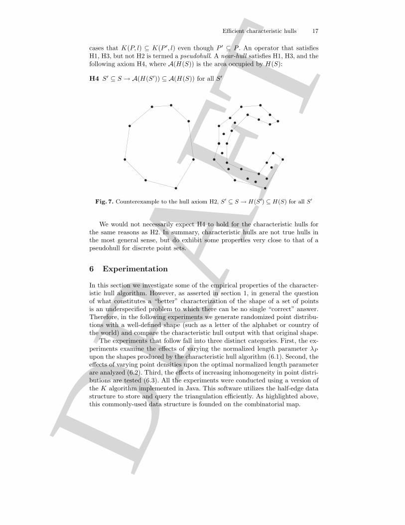
Axiom H2 may not be a desirable goal for characteristic hulls. For example,Figure 7 shows that a superset of S can provide more information about theshape of a region. In direct contradiction to H2, it may be desirable in many

DR

AFT


cases that K(P, l) ⊆ K(P ′, l) even though P ′ ⊆ P . An operator that satisfiesH1, H3, but not H2 is termed a pseudohull. A near-hull satisfies H1, H3, and thefollowing axiom H4, where A(H(S)) is the area occupied by H(S):

H4 S′ ⊆ S → A(H(S′)) ⊆ A(H(S)) for all S′

Fig. 7. Counterexample to the hull axiom H2, S′ ⊆ S → H(S′) ⊆ H(S) for all S′

We would not necessarily expect H4 to hold for the characteristic hulls forthe same reasons as H2. In summary, characteristic hulls are not true hulls inthe most general sense, but do exhibit some properties very close to that of apseudohull for discrete point sets.

6 Experimentation

In this section we investigate some of the empirical properties of the character-istic hull algorithm. However, as asserted in section 1, in general the questionof what constitutes a “better” characterization of the shape of a set of pointsis an underspecified problem to which there can be no single “correct” answer.Therefore, in the following experiments we generate randomized point distribu-tions with a well-defined shape (such as a letter of the alphabet or country ofthe world) and compare the characteristic hull output with that original shape.

The experiments that follow fall into three distinct categories. First, the ex-periments examine the effects of varying the normalized length parameter λP

upon the shapes produced by the characteristic hull algorithm (6.1). Second, theeffects of varying point densities upon the optimal normalized length parameterare analyzed (6.2). Third, the effects of increasing inhomogeneity in point distri-butions are tested (6.3). All the experiments were conducted using a version ofthe K algorithm implemented in Java. This software utilizes the half-edge datastructure to store and query the triangulation efficiently. As highlighted above,this commonly-used data structure is founded on the combinatorial map.

DR

AFT


6.1 Parameterization

Section 5.2 suggested some natural choices for parameterizing the characteristichull algorithm using the normalized length λP . In this section we examine morecarefully the response of the algorithm to changes in normalized length.

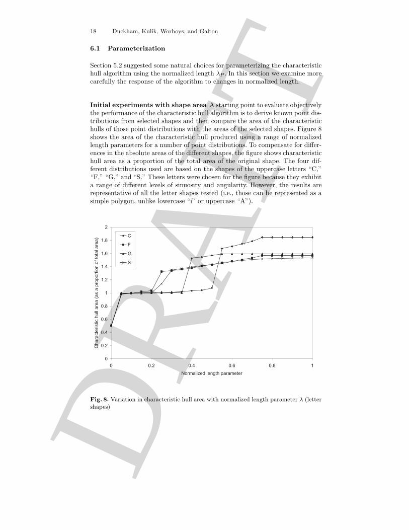
Initial experiments with shape area A starting point to evaluate objectivelythe performance of the characteristic hull algorithm is to derive known point dis-tributions from selected shapes and then compare the area of the characteristichulls of those point distributions with the areas of the selected shapes. Figure 8shows the area of the characteristic hull produced using a range of normalizedlength parameters for a number of point distributions. To compensate for differ-ences in the absolute areas of the different shapes, the figure shows characteristichull area as a proportion of the total area of the original shape. The four dif-ferent distributions used are based on the shapes of the uppercase letters “C,”“F,” “G,” and “S.” These letters were chosen for the figure because they exhibita range of different levels of sinuosity and angularity. However, the results arerepresentative of all the letter shapes tested (i.e., those can be represented as asimple polygon, unlike lowercase “i” or uppercase “A”).

0

0.2

0.4

0.6

0.8

1

1.2

1.4

1.6

1.8

2

0 0.2 0.4 0.6 0.8 1

Normalized length parameter

Ch

ara

cte

ristic

hu

lla

rea

(as

ap

rop

ort

ion

of

tota

la

rea

) C

F

G

S

Fig. 8. Variation in characteristic hull area with normalized length parameter λ (lettershapes)

DR

AFT


The letter shapes were generated using a sans serif font (Arial). The boundaryof each shape was approximated as a polygon using a number of evenly spacedvertices connected by straight-line segments. Each shape was then filled with asemi-random distribution of internal points, where each point must be greaterthan a certain threshold distance d from any other points, but otherwise israndomly positioned. Truly random distributions of points can have stronglyinhomogeneous densities, leading to the formation of clusters and holes whichmask the true shape of the letter itself. Hence, the semi-random distribution wasused for these initial experiments.

Together the polygon vertices and the internal points compose the input pointset. For each shape, 20 semi-random internal point sets were generated, ensuringrandomized, but reasonably evenly spaced input point set distributions. Figure8 shows the average area of these 20 distributions for each shape at each of 21normalized length parameters (0.0, 0.05, 0.1, ..., 1.0). Thus, figure 8 summarizesthe properties of a total of 4 × 21 × 20 = 1680 different characteristic hulls.

As expected, Figure 8 shows that the area of figures decreases monotonicallywith decreasing normalized length: the shorter the length parameter, the moreedges can be removed from the triangulation, and so the smaller the total areaof the feature. The response curves for the different figures also exhibit a numberof pronounced “steps.” These steps correspond to the removal of a small numberof triangles with relatively large areas from the triangulation (for example thosethat make up the interior of the triangulated “C” shape, as in Figure 5).

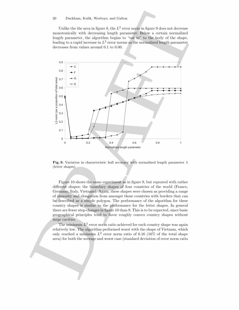
Experiments with L2 error norm Using the ratio of characteristic hull areato original shape is simple but does not provide a particularly good measureof closeness of the two shapes. Two very different shapes can still have thesame area. For this reason it is preferable to use the L2 error norm: the areaof the region enclosed between the boundaries of the original shape and thecorresponding characteristic hull. An L2 error norm of zero means that not onlyare the areas of the two shapes equal, but also that their boundaries are incomplete agreement. Figure 9 was generated using the same points sets as figure8, but shows variation in the L2 error norm with normalized length parameter.Again, the L2 error norm values are shown as a proportion of the total shapearea, to compensate for differences in the absolute values of the areas of thedifferent shapes.

As in figure 8, figure 9 shows a number of large “steps” corresponding tothe removal of large cavities in the triangulated shapes. All the shapes haveresponse curves that reach a minimum L2 error norm ratio of less than 0.06(i.e., the total area of disagreement between the characteristic hull and originalshape is on average less than 6% of the total area of the shape). However, evenin the very worst cases (recall that each data point in figure 9 represents anaverage of the characteristic hulls of 20 different randomized point distributions)all randomized point distributions achieved a minimum L2 error norm ratio ofless than 0.1 (10% of the total shape area).

DR

AFT


Unlike the the area in figure 8, the L2 error norm in figure 9 does not decreasemonotonically with decreasing length parameter. Below a certain normalizedlength parameter, the algorithm begins to “eat in” to the body of the shape,leading to a rapid increase in L2 error norms as the normalized length parameterdecreases from values around 0.1 to 0.00.

0

0.1

0.2

0.3

0.4

0.5

0.6

0.7

0.8

0.9

0 0.2 0.4 0.6 0.8 1


L2

-no

rm(a

sa

pro

po

rtio

no

fto

tala

rea

)

C

F

G

S

Fig. 9. Variation in characteristic hull accuracy with normalized length parameter λ(letter shapes)

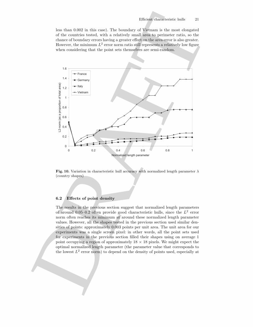
Figure 10 shows the same experiment as in figure 9, but repeated with ratherdifferent shapes: the boundary shapes of four countries of the world (France,Germany, Italy, Vietnam). Again, these shapes were chosen as providing a rangeof sinuosity and elongation from amongst those countries with borders that canbe described as a simple polygon. The performance of the algorithm for thesecountry shapes is similar to the performance for the letter shapes. In generalthere are fewer step-changes in figure 10 than 9. This is to be expected, since basicgeographical principles tend to favor roughly convex country shapes withoutlarge cavities.

The minimum L2 error norm ratio achieved for each country shape was againrelatively low. The algorithm performed worst with the shape of Vietnam, whichonly reached a minimum L2 error norm ratio of 0.16 (16% of the total shapearea) for both the average and worst case (standard deviation of error norm ratio

DR

AFT


less than 0.002 in this case). The boundary of Vietnam is the most elongatedof the countries tested, with a relatively small area to perimeter ratio, so thechance of boundary errors having a greater effect on the area error is also greater.However, the minimum L2 error norm ratio still represents a relatively low figurewhen considering that the point sets themselves are semi-random.

0

0.2

0.4

0.6

0.8

1

1.2

1.4

1.6

0 0.2 0.4 0.6 0.8 1


L2

-no

rm(a

sa

pro

po

rtio

no

fto

tala

rea

)

France

Germany

Italy

Vietnam

Fig. 10. Variation in characteristic hull accuracy with normalized length parameter λ(country shapes)

6.2 Effects of point density

The results in the previous section suggest that normalized length parametersof around 0.05–0.2 often provide good characteristic hulls, since the L2 errornorm often reaches its minimum at around these normalized length parametervalues. However, all the shapes tested in the previous section used similar den-sities of points: approximately 0.003 points per unit area. The unit area for ourexperiments was a single screen pixel: in other words, all the point sets usedfor experiments in the previous section filled their shapes using on average 1point occupying a region of approximately 18 × 18 pixels. We might expect theoptimal normalized length parameter (the parameter value that corresponds tothe lowest L2 error norm) to depend on the density of points used, especially at

DR

AFT


lower point densities where the number of points used to define the same shapeis much lower.

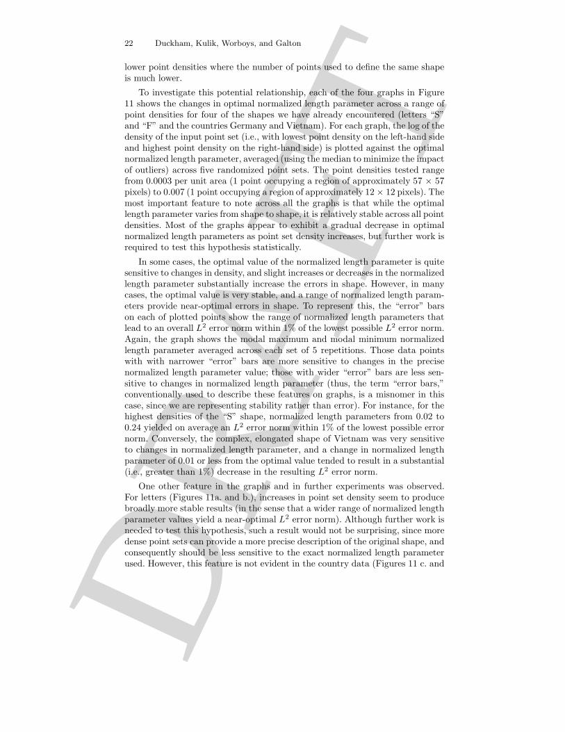
To investigate this potential relationship, each of the four graphs in Figure11 shows the changes in optimal normalized length parameter across a range ofpoint densities for four of the shapes we have already encountered (letters “S”and “F” and the countries Germany and Vietnam). For each graph, the log of thedensity of the input point set (i.e., with lowest point density on the left-hand sideand highest point density on the right-hand side) is plotted against the optimalnormalized length parameter, averaged (using the median to minimize the impactof outliers) across five randomized point sets. The point densities tested rangefrom 0.0003 per unit area (1 point occupying a region of approximately 57 × 57pixels) to 0.007 (1 point occupying a region of approximately 12 × 12 pixels). Themost important feature to note across all the graphs is that while the optimallength parameter varies from shape to shape, it is relatively stable across all pointdensities. Most of the graphs appear to exhibit a gradual decrease in optimalnormalized length parameters as point set density increases, but further work isrequired to test this hypothesis statistically.

In some cases, the optimal value of the normalized length parameter is quitesensitive to changes in density, and slight increases or decreases in the normalizedlength parameter substantially increase the errors in shape. However, in manycases, the optimal value is very stable, and a range of normalized length param-eters provide near-optimal errors in shape. To represent this, the “error” barson each of plotted points show the range of normalized length parameters thatlead to an overall L2 error norm within 1% of the lowest possible L2 error norm.Again, the graph shows the modal maximum and modal minimum normalizedlength parameter averaged across each set of 5 repetitions. Those data pointswith with narrower “error” bars are more sensitive to changes in the precisenormalized length parameter value; those with wider “error” bars are less sen-sitive to changes in normalized length parameter (thus, the term “error bars,”conventionally used to describe these features on graphs, is a misnomer in thiscase, since we are representing stability rather than error). For instance, for thehighest densities of the “S” shape, normalized length parameters from 0.02 to0.24 yielded on average an L2 error norm within 1% of the lowest possible errornorm. Conversely, the complex, elongated shape of Vietnam was very sensitiveto changes in normalized length parameter, and a change in normalized lengthparameter of 0.01 or less from the optimal value tended to result in a substantial(i.e., greater than 1%) decrease in the resulting L2 error norm.

One other feature in the graphs and in further experiments was observed.For letters (Figures 11a. and b.), increases in point set density seem to producebroadly more stable results (in the sense that a wider range of normalized lengthparameter values yield a near-optimal L2 error norm). Although further work isneeded to test this hypothesis, such a result would not be surprising, since moredense point sets can provide a more precise description of the original shape, andconsequently should be less sensitive to the exact normalized length parameterused. However, this feature is not evident in the country data (Figures 11 c. and

DR

AFT


d.), and if anything the converse seems to be true. We attribute this counter-intuitive feature to the experimental design, where the boundary of the originalshape is sub-sampled using evenly spaced points at the current point density.The fractal properties of many real world shapes including country boundaries(e.g., [16, 19]) means that, unlike non-fractal letter shapes, this sub-samplingcauses increased detail to be revealed at each increased level of density, poten-tially masking some of the trends otherwise associated with increasing point setdensity. Future work will address this issue.

0

0.05

0.1

0.15

0.2

0.25

-3.5 -3.3 -3.1 -2.9 -2.7 -2.5 -2.3 -2.1

Density of point set (log of points per unit area)

Op

tim

al

no

rmalized

len

gth

para

mete

r

0

0.05

0.1

0.15

0.2

0.25

-3.5 -3.3 -3.1 -2.9 -2.7 -2.5 -2.3 -2.1


Op

tim

al

no

rmalized

len

gth

para

mete

r

a. Letter “S” b. Letter “F”

0

0.05

0.1

0.15

0.2

0.25

-3.5 -3.3 -3.1 -2.9 -2.7 -2.5 -2.3 -2.1


Op

tim

al

no

rmalized

len

gth

para

mete

r

0

0.05

0.1

0.15

0.2

0.25

-3.5 -3.3 -3.1 -2.9 -2.7 -2.5 -2.3 -2.1


Op

tim

al

no

rmalized

len

gth

para

mete

r

c. Germany d. Vietnam

Fig. 11. Effects of changing density of input point set on optimal normalized lengthparameter

6.3 Effects of point distribution

Finally, as discussed at the beginning of section 6, all the point distributions sofar were semi-randomly distributed (position is random, subject to a minimumdistance between any two pairs of points). Thus, while the point distributionsused were randomized, the distribution of points was homogeneous, as illustratedby the point distributions in figure 1. They are “dot patterns” in the sense of [7].A truly random distribution of points will exhibit clusters that are expected to

DR

AFT


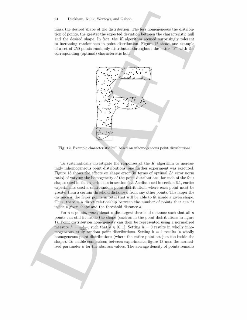
mask the desired shape of the distribution. The less homogeneous the distribu-tion of points, the greater the expected deviation between the characteristic hulland the desired shape. In fact, the K algorithm seemed surprisingly tolerantto increasing randomness in point distribution. Figure 12 shows one exampleof a set of 250 points randomly distributed throughout the letter “F” with thecorresponding (optimal) characteristic hull.

Fig. 12. Example characteristic hull based on inhomogeneous point distributions

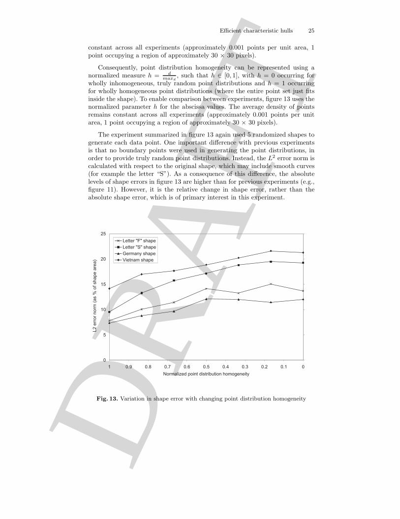
To systematically investigate the responses of the K algorithm to increas-ingly inhomogeneous point distributions, one further experiment was executed.Figure 13 shows the effects on shape error (in terms of optimal L2 error normratio) of varying the homogeneity of the point distributions, for each of the fourshapes used in the experiments in section 6.2. As discussed in section 6.1, earlierexperiments used a semi-random point distribution, where each point must begreater than a certain threshold distance d from any other points. The larger thedistance d, the fewer points in total that will be able to fit inside a given shape.Thus, there is a direct relationship between the number of points that can fitinside a given shape and the threshold distance d.

For a n points, maxd denotes the largest threshold distance such that all npoints can still fit inside the shape (such as in the point distributions in figure1). Point distribution homogeneity can then be represented using a normalizedmeasure h = d

maxd, such that h ∈ [0, 1]. Setting h = 0 results in wholly inho-

mogeneous, truly random point distributions. Setting h = 1 results in whollyhomogeneous point distributions (where the entire point set just fits inside theshape). To enable comparison between experiments, figure 13 uses the normal-ized parameter h for the abscissa values. The average density of points remains

DR

AFT


constant across all experiments (approximately 0.001 points per unit area, 1point occupying a region of approximately 30 × 30 pixels).

Consequently, point distribution homogeneity can be represented using anormalized measure h = d

maxd, such that h ∈ [0, 1], with h = 0 occurring for

wholly inhomogeneous, truly random point distributions and h = 1 occurringfor wholly homogeneous point distributions (where the entire point set just fitsinside the shape). To enable comparison between experiments, figure 13 uses thenormalized parameter h for the abscissa values. The average density of pointsremains constant across all experiments (approximately 0.001 points per unitarea, 1 point occupying a region of approximately 30 × 30 pixels).

The experiment summarized in figure 13 again used 5 randomized shapes togenerate each data point. One important difference with previous experimentsis that no boundary points were used in generating the point distributions, inorder to provide truly random point distributions. Instead, the L2 error norm iscalculated with respect to the original shape, which may include smooth curves(for example the letter “S”). As a consequence of this difference, the absolutelevels of shape errors in figure 13 are higher than for previous experiments (e.g.,figure 11). However, it is the relative change in shape error, rather than theabsolute shape error, which is of primary interest in this experiment.

0

5

10

15

20

25

00.10.20.30.40.50.60.70.80.91

Normalized point distribution homogeneity

L2

err

or

no

rm(a

s%

of

sh

ap

ea

rea

)

Letter "F" shape

Letter "S" shape

Germany shape

Vietnam shape

Fig. 13. Variation in shape error with changing point distribution homogeneity

DR

AFT


As expected, figure 13 does show an increase in errors with increasinglyrandom point distributions across all shapes tested. However, the magnitudeof increasing errors is relatively low, with truly random distributions typicallyincreasing the error rates by about 50% when compared with homogeneous pointdistributions. In effect, these results indicate that the K algorithm degradesgracefully in the presence of inhomogeneous point distributions. To provide somecontext for this statement, we note that the convex hulls of the four shapes infigure 13 are associated with L2 error norm ratios ranging from approximately17% (for Germany shape) through approximately 54% (for the letters “F” and“S”) to more than 150% (for Vietnam shape). Even using truly random pointdistributions, the characteristic hulls for these shapes yield error norm ratiosbetween 12% (for Germany shape) through to 21% (for Vietnam shape).

6.4 Discussion of experimental results

In summary, the experimental evaluation of the K algorithm yielded the follow-ing key results:

– The K algorithm is able to accurately characterize the shape of point setsderived from a range of different shape types, given appropriate parameter-ization.

– Although the optimal parameter value varies for different shapes and pointdistributions, normalized parameter values of between 0.05–0.2 typically pro-duce optimal or near-optimal shape characterization across a wide range ofpoint distributions.

– The optimal parameter value algorithm is relatively stable in the presence ofchanges in point density and changing point distribution homogeneity (fromsemi-random to truly random).

7 Conclusions

In this paper we have presented a new algorithm for generating a simple, con-nected, possibly non-convex polygon that characterizes the shape of a set ofpoints in the plane. The algorithm, based on the Delaunay triangulation of thepoint set, is optimal, requiring O(n log n) time to execute. The shape producedby our algorithm is parameterized by means of a single normalized length param-eter. Changing the length parameter produces a finite family of characteristichulls ranging from the convex hull at one extreme to a uniquely defined simplepolygon with minimal area at the other extreme.

No one parameter value can ever yield a “correct” answer; instead differentparameter values are expected to be required for different applications. However,some guidelines for good lengths are suggested by experiments using the algo-rithm. Experimental results further demonstrate the algorithm’s stability andgraceful degradation across a wide range of input point sets. A variety of furtherexperimental work is suggested by this research. Two specific issues mentionedin (section 6.2) that warrant further systematic investigation are:

DR

AFT


– the hypothesized decrease in optimal normalized length parameter with in-creasing point set density; and

– the hypothesized increase in optimal normalized length parameter stabilitywith increasing point set density.

More generally, experiments to evaluate the performance of the K algorithmacross a wider range of shapes and in comparison to the other shape character-ization algorithms reviewed in section 2 would certainly be beneficial.

Extensions of the algorithm to higher dimensions are also possible. How-ever, a direct extension to three-dimensional space does present efficiency prob-lems. In particular, since in three dimensions any number of exterior faces of aregular three-dimensional triangulation could meet at a single vertex, a three-dimensional regularity check algorithm in would be expected to require substan-tially more computation.

Acknowledgments

Glenn Hudson developed the Java software used to run the experiments describedin this paper and provided helpful feedback and comments on the algorithmitself.

References

1. Harith Alani, Christopher B. Jones, and Douglas Tudhope. Voronoi-based regionapproximation for geographical information retrieval with gazetteers. InternationalJournal of Geographical Information Science, 15(4):287–306, 2001.

2. Nina Amenta, Sunghee Choi, and Ravi Kolluri. The power crust. In Sixth ACMSymposium on Solid Modeling and Applications, pages 249–260, 2001.

3. Nina Amenta, Sunghee Choi, and Ravi Kolluri. The power crust, unions of balls,and the medial axis transform. Computational Geometry: Theory and Applications,19(2–3):127–153, 2001.

4. Avi Arampatzis, Marc van Kreveld, Iris Reinbacher, Christopher B. Jones,Subodh Vaid, Paul Clough, Hideo Joho, Mark Sanderson, Mark Benkert,and Alexander Wolff. Web-based delineation of imprecise regions. InWorkshop on Geographic Information Retrieval (SIGIR 2004), 2004.(http://www.geo.unizh.ch/˜rsp/gir/abstracts/arampatzis.pdf, accessed 8/7/05).

5. D. Attali. r-regular shape reconstruction from unorganised points. ComputationalGeometry, 10:239–47, 1998.

6. B. Baumgart. A polyhedron representation for computer vision. In Proc. AFIPSNational Computer Conference, volume 44, pages 589–596, 1975.

7. A. R. Chaudhuri, B. B. Chaudhuri, and S. K. Parui. A novel approach to com-putation of the shape of a dot pattern and extraction of its perceptual border.Computer Vision and Image Understanding, 68(3):257–275, 1997.

8. B. Chazelle. On the convex layers of a planar set. IEEE Transactions on Infor-mation Theory, 31:509–517, 1985.

9. Jean-Francois Dufourd and Francois Puitg. Functional specification and proto-typing with oriented combinatorial maps. Computation Geometry—Theory andApplications, 16(2):129–156, 2000.

DR

AFT


10. Herbert Edelsbrunner, David G. Kirkpatrick, and Raimund Seidel. On the shapeof a set of points in the plane. IEEE Transactions on Information Theory, IT–29(4):551–559, 1983.

11. J.R. Edmonds. A combinatorial representation for polyhedral surfaces. Notices ofthe American Mathematical Society, 7:646, 1960.

12. M. J. Fadili, M. Melkemi, and A. ElMoataz. Non-convex onion-peeling using ashape hull algorithm. Pattern Recognition Letters, 25:1577–1585, 2004.

13. A. Galton and M. Duckham. What is the region occupied by a set of points?In GIScience, volume 4197 of Lecture Notes in Computer Science, pages 81–98.Springer, 2006.

14. Gautam Garai and B. B. Chaudhuri. A split and merge procedure for polygonalborder detection of dot pattern. Image and Vision Computing, 17:75–82, 1999.

15. R. Klette and A. Rosenfeld. Digital geometry: Geometric Methods for Digital ImageAnalysis. Morgan Kaufmann, 2004.

16. B. B. Mandelbrot. How long is the coast of Great Britain: Statistical self similarityand fractional dimension. Science, 155:636–638, 1967.

17. Mahmoud Melkemi and Mourad Djebali. Computing the shape of a planar pointsset. Pattern Recognition, 33:1423–1436, 2000.

18. J. O’Rourke. Computational geometry in C. Cambridge University Press, Cam-bridge, UK, 2nd edition, 1998.

19. L. F. Richardson. The problem of contiguity: An appendix of statistics of deadlyquarrels. General Systems Yearbook, 6:139–187, 1961.

20. K. Weiler. Edge-based data structures for solid modeling in curved-surface envi-ronments. Computer Graphics and Applications, 5(1):21–40, 1985.

eﬃcient characteristic hulls - geosensor.net

Documents