east garrington gas plant looking northeast towards the trench
TRANSCRIPT

East Garrington Gas Plant Looking Northeast Towards the
Trench and Gate Research Site

THE UNIVERSITY OF CALGARY
The Trench and Gate Groundwater
Remediation System
by
Marc W. Bowles
A THESIS
SUBMITTED TO THE FACULTY OF GRADUATE STUDIES
IN PARTIAL FULFILMENT OF THE REQUIREMENTS FOR THE
DEGREE OF MASTER OF SCIENCE
DEPARTMENT OF GEOLOGY & GEOPHYSICS
CALGARY, ALBERTA
NOVEMBER, 1997
Marc W. Bowles 1997

ii
THE UNIVERSITY OF CALGARY
FACULTY OF GRADUATE STUDIES
The undersigned certify that they have read, and recommend to the Faculty of Graduate
Studies for acceptance, a thesis entitled “The Trench and Gate Groundwater Remediation
System” submitted by Marc W. Bowles in partial fulfilment of the requirements for the
degree of Master of Science.
Supervisor, Dr. Laurence R. BentleyDepartment of Geology and Geophysics
Dr. Cathy RyanDepartment of Geology and Geophysics
Dr. Angus ChuDepartment of Civil Engineering
Date

iii
ABSTRACT
Funnel and Gate technologies are inappropriate for remediating groundwater
contamination in low permeability sediments like glacial tills, because the design produces
mounding effects which force flow underneath and around funnel walls.
The Trench and Gate is a modified Funnel and Gate system suitable for installation in tills.
Modifications include the addition of high hydraulic conductivity trenches along the up-
gradient side of the funnel walls and a reinfiltration gallery down-gradient of the treatment
gate. Preferential groundwater flow through the added high permeability infrastructure
prevents mounding and induces a capture zone both horizontally, and vertically larger than
the cross-sectional funnel area. Coupled with bioremediation catalyzed by biosparging, or
other remediation technologies, the system constitutes an economical, in-situ, long-term
contaminant plume capture and treatment method, suitable for low to moderate
permeability sediments. A prototype Trench and Gate was successfully installed at the
East Garrington Gas Plant, Alberta, Canada.

iv
ACKNOWLEDGEMENTS
I gratefully acknowledge funding for this research project provided by Amoco Canada
Petroleum Company Ltd., the Canadian Association of Petroleum Producers (CAPP), the
Groundwater and Soil Remediation Program (GASReP), the Natural Sciences
Engineering and Research Council of Canada - Industry Oriented Research (NSERC-IOR)
program, and Shell Research Ltd.. Additional support in the form of research personnel
and facilities, as well as in-kind or at-cost contributions has been provided by Komex
International Ltd., Quest, An Alliance Corporation, The University of Calgary, The
Waterloo Centre for Groundwater Research, Maxxam Analytics Inc. (formerly Chemex
Labs Alberta Inc.), Rice Engineering Ltd., and Nilex Inc..
I sincerely appreciate the guidance of my advisor Dr. Laurence Bentley and the
contribution of thesis reviewers Dr. Cathy Ryan and Dr. Angus Chu.
I wish to thank Tom Houseman, Kelly Johnson, and Tom Sharkey of Amoco for letting
me use “their” East Garrington Gas Plant for the research. Fellow researchers Dr. Jim
Barker, David Granger, Bill Hoyne, Helen Jacobs, and David Thomas all contributed to
the success of this project.
The staff at Komex provided superior technical, data management, drafting, engineering,
and field support. Shawn Rimbey and Francine Forrest provided invaluable aid in
designing and conducting the experiment to isolate and identify the hydrocarbon degrading
bacteria (Section 5.2.1). Allan Shea, Mike Thompson, and Jeff Rathgeber oversaw the
engineering design and technical drawing preparation. I offer my sincere thanks to all of
you, and to Tad who made me do it.

v
DEDICATION
This thesis is dedicated to my loving wife Wendy and our supportive children Jill,
Timothy, and Ross who spent too many weekends and evenings without “Dad” so that the
theory could become a reality.

vi
TABLE OF CONTENTS
Page No.
FrontispieceApproval Page.................................................................................................................iiAbstract..........................................................................................................................iiiAcknowledgements......................................................................................................... ivDedication ....................................................................................................................... vTable of Contents ........................................................................................................... viList of Tables................................................................................................................viiiList of Figures ................................................................................................................ ixList of Drawings ............................................................................................................. xiList of Appendices......................................................................................................... xiiEpigraph.......................................................................................................................xiii
1. INTRODUCTION .....................................................................................................11.1 BACKGROUND ...................................................................................................................11.2 RATIONALE .......................................................................................................................11.3 SITE SELECTION AND HISTORY ..........................................................................................41.4 PROJECT OBJECTIVE..........................................................................................................51.5 PREVIOUS RESEARCH ........................................................................................................8
1.5.1 Groundwater Flow in Till ....................................................................................................... 81.5.2 Hydrocarbon Biodegradation ................................................................................................ 101.5.3 Funnel and Gate ................................................................................................................... 11
2. SITE CHARACTERIZATION............................................................................... 132.1 CLIMATE AND PHYSIOGRAPHY ........................................................................................ 132.2 BEDROCK GEOLOGY........................................................................................................ 142.3 SURFICIAL DEPOSITS ....................................................................................................... 162.4 GROUNDWATER MONITORING NETWORK ........................................................................ 23
3. HYDRAULIC CONDUCTIVITY TESTING......................................................... 263.1 LABORATORY TESTS ....................................................................................................... 263.2 PIEZOMETER TESTS......................................................................................................... 273.3 EXPERIMENTAL TRENCH HYDRAULIC CONDUCTIVITY TESTING ....................................... 29
3.3.1 Test Design .......................................................................................................................... 293.3.2 Test Results .......................................................................................................................... 32
3.4 PREDICTING TREATMENT FLUXES FROM BULK HYDRAULIC CONDUCTIVITIES ................. 38

vii
TABLE OF CONTENTS (Continued)
Page No.
4. HYDROGEOLOGY................................................................................................ 404.1 REGIONAL HYDROGEOLOGY............................................................................................ 404.2 SITE HYDROGEOLOGY ..................................................................................................... 43
4.2.1 Groundwater Flow................................................................................................................ 434.2.2 Groundwater Type................................................................................................................ 44
4.3 CONTAMINANT HYDROGEOLOGY .................................................................................... 464.3.1 Contaminant Sources, Types, and Distribution ..................................................................... 464.3.2 Contaminant Behaviour in Groundwater............................................................................... 48
5. TRENCH AND GATE.............................................................................................. 505.1 HYDRAULICS AND DESIGN............................................................................................... 50
5.1.1 Theory and Conceptual Design ............................................................................................. 505.1.2 Engineering Design.............................................................................................................. 545.1.3 Installation ........................................................................................................................... 59
5.2 TREATMENT OF CONTAMINATED GROUNDWATER ........................................................... 615.2.1 Isolation and Identification of Hydrocarbon Degrading Bacterial Species.............................. 615.2.2 Biodegradation and Nutrient Amendment Experiments ........................................................ 65
6. DISCUSSION .......................................................................................................... 686.1 HYDRAULIC EVALUATION ............................................................................................... 68
6.1.1 Computer Groundwater Modelling ....................................................................................... 686.1.2 Hydraulic Response to Infiltration Events ............................................................................. 726.1.3 Calculating Bulk Hydraulic Conductivity from Measured Flux ............................................. 766.1.4 Field Measurement of Potentiometric Surfaces...................................................................... 77
6.2 HYDROCHEMICAL EVALUATION ...................................................................................... 806.2.1 Field Procedures and Analytical Techniques......................................................................... 806.2.2 Field Measured Parameters................................................................................................... 856.2.3 Laboratory Analytical Data................................................................................................... 87
6.3 PERFORMANCE EVALUATION........................................................................................... 93
7. CONCLUSIONS...................................................................................................... 95
8. REFERENCES ........................................................................................................ 97

viii
LIST OF TABLES
Page No.
TABLE 2-1 TERRAIN UNITS IN THE EAST GARRINGTON AREA .......................................... 19TABLE 2-2 X-RAY DIFFRACTION ANALYSES................................................................... 20TABLE 3-1 PERMEAMETER HYDRAULIC CONDUCTIVITY TEST RESULTS........................... 26TABLE 3-2 SUMMARY OF DRAWDOWN-DERIVED HYDRAULIC CONDUCTIVITIES.............. 29TABLE 4-1 PHYSICAL AND CHEMICAL PROPERTIES OF BTEX COMPOUNDS ..................... 48TABLE 5-1 GROWTH RESULTS MATRIX FOR BACTERIA.................................................... 63TABLE 6-1 ANALYTICAL METHODS SUMMARY ............................................................... 83TABLE 6-2 DISSOLVED OXYGEN VALUES (mg/L) IN INFILTRATION GALLERY
PIEZOMETERS ............................................................................................... 87

ix
LIST OF FIGURESPage No.
FIGURE 1-1 PLAN VIEW SCHEMATIC COMPARISON OF FUNNEL AND GATE AND
TRENCH AND GATE GROUNDWATER REMEDIATION SYSTEMS..........................3FIGURE 1-2 EAST GARRINGTON GAS PLANT LOCATION MAP (LSD 11-17-34-3 W5M)......5FIGURE 1-3 LOCATION, TOPOGRAPHY, AND DRAINAGE MAP. ...........................................6FIGURE 2-1 BEDROCK GEOLOGY (OZORAY AND BARNES, 1977). .................................... 15FIGURE 2-2 REGIONAL SURFICIAL GEOLOGY (SHETSON, 1987). ...................................... 17FIGURE 2-3 ANNOTATED AIR PHOTO OF THE EAST GARRINGTON AREA. .......................... 18FIGURE 2-4 INTERPRETED SCHEMATIC CROSS-SECTION OF THE QUATERNARY GEOLOGY
IN THE VICINITY OF THE EAST GARRINGTON PLANT SITE (LOOKING
NORTHWEST). ............................................................................................. 19FIGURE 2-5 SITE PLAN OF THE EAST GARRINGTON GAS PLANT. ...................................... 21FIGURE 2-6 ELECTROMAGNETIC (EM-38) MAP OF THE NORTHEAST CORNER OF THE
EAST GARRINGTON SITE.............................................................................. 23FIGURE 2-7 HYDROGEOLOGICAL CROSS-SECTION A-A’. ................................................. 24FIGURE 3-1 SCHEMATIC OF TRENCH PUMPING TEST LAYOUT. ......................................... 30FIGURE 3-2 DRAWDOWN WITHIN THE TRENCH AND PIEZOMETERS DURING THE TRENCH
PUMPING TEST. ........................................................................................... 31FIGURE 3-3 DRAWDOWN VS. TIME FOR MONITORING WELL MW-1. ............................... 32FIGURE 3-4 DRAWDOWN VS. TIME FOR PIEZOMETER 16B. .............................................. 32FIGURE 3-5 DRAWDOWN VS. TIME FOR MONITORING WELL MW-1................................. 34FIGURE 4-1 REGIONAL HYDROGEOLOGICAL MAP SHOWING LOCATIONS OF
HYDROGEOLOGICAL CROSS-SECTIONS (OZORAY AND BARNES, 1977). ........ 40FIGURE 4-2 HYDROGEOLOGICAL LEGEND TO ACCOMPANY REGIONAL HYDRO-
GEOLOGICAL MAPS AND CROSS-SECTIONS (OZORAY AND BARNES, 1977).... 41FIGURE 4-3 REGIONAL HYDROGEOLOGICAL CROSS-SECTION B-B’(OZORAY AND
BARNES, 1977). .......................................................................................... 42FIGURE 4-4 REGIONAL HYDROGEOLOGICAL CROSS-SECTION C-C’ (OZORAY AND
BARNES, 1977). .......................................................................................... 42FIGURE 4-5 EXPANDED DUROV DIAGRAM. ..................................................................... 45FIGURE 5-1 EFFECT OF HIGH PERMEABILITY ZONE ON GROUNDWATER FLOW (AFTER
BEAR, 1979). .............................................................................................. 50FIGURE 5-2 SCHEMATIC OF TRENCH AND GATE DESIGN. .................................................. 51FIGURE 5-3 PLAN VIEW SCHEMATIC COMPARISON OF FLOW LINES AND CAPTURE ZONES
FOR THE FUNNEL AND GATE AND TRENCH AND GATE SYSTEMS. .................... 53FIGURE 5-4 CROSS-SECTION SCHEMATIC COMPARISON OF FLOW LINES AND CAPTURE
ZONES FOR THE FUNNEL AND GATE AND TRENCH AND GATE SYSTEMS. ......... 53FIGURE 5-5 SCHEMATIC CROSS-SECTION OF TRENCH CONSTRUCTION DETAILS............... 54FIGURE 5-6 SCHEMATIC OF “L” SHAPED MONITORING WELL ARRANGEMENT. ................ 55FIGURE 5-7 PLAN VIEW OF CULVERT ARRANGEMENT. .................................................... 57FIGURE 5-8 INFILTRATION GALLERY AND TRENCH LAYOUT. ........................................... 58

x
LIST OF FIGURES (Continued)Page No.
FIGURE 5-9 SCHEMATIC DIAGRAM OF EXPERIMENTAL GATE TREATMENT SYSTEM
(GRANGER, 1997). ...................................................................................... 65FIGURE 5-10 PLAN VIEW OF NUTRIENT AMENDMENT SYSTEM IN THE SECOND GATE
(GRANGER, 1997). ...................................................................................... 66FIGURE 6-1 PLAN VIEW OF FLOW FIELD FOR THE TRENCH AND GATE SYSTEM
(HOYNE, IN PREP.). ..................................................................................... 69FIGURE 6-2 PLAN VIEW OF THE POTENTIOMETRIC SURFACE AND FLOW VECTORS FOR
THE TRENCH AND GATE SYSTEM (HOYNE, IN PREP.). ..................................... 70FIGURE 6-3 THREE DIMENSIONAL REPRESENTATION OF FLOW FIELD IN THE TRENCH AND
GATE SYSTEM (HOYNE, IN PREP.)................................................................. 71FIGURE 6-4 PLAN VIEW OF FLOW FIELD FOR THE FUNNEL AND GATE SYSTEM (HOYNE,
IN PREP.). .................................................................................................... 72FIGURE 6-5 HYDROGRAPHS OF RESPONSE TO MELTING AND INFILTRATION EVENTS
(THOMAS, IN PREP.)..................................................................................... 74FIGURE 6-6 CORRELATION BETWEEN MEASURED FLOW RATES THROUGH THE GATE AND
PRECIPITATION (THOMAS, IN PREP.)............................................................. 75FIGURE 6-7 CHANGES IN VERTICAL HYDRAULIC GRADIENT IN RESPONSE TO
PRECIPITATION EVENTS (THOMAS, IN PREP.)................................................ 76FIGURE 6-8 PRE-TRENCH AND GATE UPPERMOST GROUNDWATER-BEARING ZONE
POTENTIOMETRIC CONTOURS, DECEMBER, 1994. ........................................ 77FIGURE 6-9 PRE-TRENCH AND GATE UPPERMOST GROUNDWATER-BEARING ZONE
POTENTIOMETRIC CONTOURS, JUNE, 1995. .................................................. 78FIGURE 6-10 POST-TRENCH AND GATE UPPERMOST GROUNDWATER-BEARING ZONE
CONTOURS, FEBRUARY, 1996................................................................... 78FIGURE 6-11 POST-TRENCH AND GATE UPPERMOST GROUNDWATER-BEARING ZONE
POTENTIOMETRIC CONTOURS, OCTOBER, 1996. ........................................ 79FIGURE 6-12 TEMPORAL VARIATION IN PH FOR CULVERT WELLS 1, 2, AND 7. ................ 86FIGURE 6-13 TEMPORAL VARIATION IN DISSOLVED IRON CONCENTRATIONS FOR
CULVERT WELLS 1, 2, AND 7. ................................................................... 91

xi
LIST OF DRAWINGSLocation
DRAWING 1 Trench & Gate Piping Details ................................................. In PocketDRAWING 2 Trench & Gate Civil Details .................................................... In Pocket

xii
LIST OF APPENDICESPage No.
APPENDIX I Borehole Logs and Piezometer Construction Details ..................... 104APPENDIX II Hydraulic Conductivity Data and Calculations .............................. 140APPENDIX III Hydrogeological and Chemical Data Tables ................................... 188
TABLE 1 Piezometer Installation Details, Datum/Groundwater SurfaceElevations, and Hydraulic Conductivities................................... 189
TABLE 2 Field Measured Parameters ....................................................... 233TABLE 3 Major Ion Groundwater Characterization and Mineralization..... 247TABLE 4 Dissolved Hydrocarbons and Dissolved Organic Carbon............ 256TABLE 5 Indicators of Contamination, Biodegradation, and Nutrients ...... 278TABLE 6 Dissolved Metals....................................................................... 287
APPENDIX IV Construction Techniques and Schedule.......................................... 291

xiii
“Let a man profess to have discovered some new Patent Powder Pimperlimplimp, a single
pinch of which being thrown into each corner of a field will kill every bug throughout its
whole extent, and people will listen to him with attention and respect. But tell them of any
simple common sense plan, based on correct scientific principles, to check and keep within
reasonable bounds the insect foes of the farmer, and they will laugh you to scorn.”
Benjamin Walsh
The Practical Entomologist
1866
“Anybody else want to negotiate?”
Bruce Willis
The Fifth Element
1997

1
1. INTRODUCTION
1.1 BACKGROUND
Contamination of shallow groundwater by petroleum hydrocarbons and other
contaminants has become one of the most serious problems facing the oil and gas and
other industries. At numerous facilities throughout the world, contaminated groundwater
is hosted by fine-grained deposits such as silt and clay glacial tills. To date, effective and
economical treatment of contamination in these low hydraulic conductivity media has been
hampered by slow average linear groundwater flow velocities. Capture and remediation of
groundwater in these types of sediments is problematic, and in some instances, treatment
of till-borne contaminated groundwater is considered cost prohibitive. Thus, there is an
obvious need for an economical and practical method for remediating groundwater in low
permeability sediments and preventing off-site migration of contaminants.
1.2 RATIONALE
Recently, many advances have been made in the field of hydrocarbon contaminated
groundwater and soil remediation. Vapour extraction, bioventing, and pump and treat systems
are all examples of effective treatment techniques. However, many of these methods are either
too expensive in terms of equipment and operating costs, or not readily adaptable to treating
groundwater contamination in tills. Thousands of hydrocarbon processing facilities in the
Canadian prairies, elsewhere in Canada, and the world, are constructed on clayey or silty
sediments, especially till. Remediation of these sites has generally been undertaken using
conventional methods such as excavation followed by land farming, thermal desorption, or
disposal to a landfill, with the expectation that removing the hydrocarbon source from the soil
will result in groundwater clean up. Direct treatment of groundwater contamination in tills has
been hampered by slow groundwater flow rates. To overcome this problem, expensive
remediation techniques such as close-spaced extraction wells and hydro-fracturing have been
employed. In other instances, treatment of the contaminated groundwater is considered not

2
practical as it is difficult to justify large scale, clean-up operations. Yet the need for some form
of groundwater remediation is recognized.
An attractive alternative to the traditional and newer remediation techniques listed above
is the use of Funnel and Gate technology (Starr and Cherry, 1994). This system uses
impermeable barriers such as sheet piling to “funnel” groundwater flow through a
treatment zone or “gate.” The in-situ method requires minimal upkeep once installed and
should prevent off site migration of contaminants. However, research on this method has
focused primarily on groundwater contamination in media with much higher hydraulic
conductivities (i.e., sand and gravel), for which several remediation techniques (e.g., pump and
treat) already exist.
A modified Funnel and Gate interception system, re-engineered for use in lower hydraulic
conductivity sediments, represents an alternative groundwater remediation technique that is
potentially a cost effective method of plume treatment and containment; both primary concerns
of regional and national regulatory agencies. The modified Funnel and Gate system, dubbed
Trench and Gate, consists of an impermeable funnel with the addition of high hydraulic
conductivity “drainage trenches” along the inside edges of the funnel, and a high permeability
down-gradient reinfiltration gallery. A comparison of the Funnel and Gate and Trench and
Gate designs is provided in Figure 1-1.
The Trench and Gate design has many advantages. The combination of a cut-off wall and
adjacent drainage trench, as compared with traditional stand alone barriers:
1. improves drainage of the contaminated zone;
2. increases the size of the capture zone; and,
3. prevents damming effects such as mounding which force contaminants
around or under funnel walls.

3
Contaminated groundwater captured in this manner can be treated by biodegradation or other
techniques as it flows through the system. In-situ treatment and the use of natural hydraulic
gradients to move the contaminants to the treatment infrastructure, ensures that on-going costs
will be minimized as compared to maintenance-intensive ex-situ remediation designs. The use
of groundwater bioremediation techniques is advantageous in that it allows for a simple
treatment system that effectively transforms both heavy and light end hydrocarbons into
innocuous products.
Figure 1-1 Plan View Schematic Comparison of Funnel and Gate andTrench and Gate Groundwater Remediation Systems.
It is envisaged that by using innovative combinations of existing technologies (i.e., Funnel and
Gate and bioremediation) coupled with unique design modifications, a practical alternative to
expensive ex-situ treatment systems for low permeability units can be designed. Such a system
could potentially be used at hundreds of contaminated sites with similar hydrogeological

4
settings. Minor modifications to the Trench and Gate treatment system will also allow for the
remediation of non-hydrocarbon contaminants (e.g., metals).
1.3 SITE SELECTION AND HISTORY
The Amoco-operated East Garrington Gas Plant is located at LSD 11-17-34-3 W5M in Red
Deer County, Alberta. The plant was constructed in 1975 and processes raw gas. Preliminary
environmental site investigations took place at the plant in 1990 and consisted of initial and
follow-up soil vapour surveys (Hazmacon, 1990a and 1990b). Survey results outlined broad
areas of concern with elevated hydrocarbon vapours. Later the same year, a series of 14
piezometers was installed as part of a hydrogeological exploration program (O'Connor, 1991).
Piezometer monitoring (O'Connor, 1992 and Komex, 1993) confirmed the presence of
dissolved BTEX (benzene, ethylbenzene, toluene, and xylenes) over much of the site and local
areas of LNAPL (light non-aqueous phase liquids) or free product.
The East Garrington site was selected for the Trench and Gate research program for the
following reasons:
1. the facility was expected to be in operation for many years, thus allowing
for consideration of a long term remediation method;
2. the facility was constructed over what was reported to be low permeability
glacial sediments;
3. reported dissolved hydrocarbon concentrations in groundwater were in
excess of Canadian drinking water guidelines (Health Canada, 1996); and,
4. potential off-site migration of dissolved hydrocarbon contaminants needed
to be prevented.

5
1.4 PROJECT OBJECTIVE
The objective of this research project was to modify the design of the Funnel and Gate
system for use in low permeability sediments such as glacial tills, thus remediating
contaminated groundwater and preventing off-site migration of contaminants. To assess
this hypothesis, a pilot-scale, modified Funnel and Gate treatment system, termed the
“Trench and Gate" remediation system was designed and installed at the Amoco-operated
East Garrington Gas Plant, Alberta (Figure 1-2 and Figure 1-3).
Figure 1-2 East Garrington Gas Plant Location Map (LSD 11-17-34-3 W5M).

6
Figure 1-3 Location, Topography, and Drainage Map.

7
Due to the ambitious nature of the project and the interrelation of a number of different
lines of research it was necessary to integrate, in the discussion that follows, project
summaries of some of the research performed by others. In particular, research synopses
are included of :
• computer groundwater flow modelling work performed by Bill Hoyne
(Hoyne in prep.) which is used to confirm that flow around the Trench
and Gate system behaves as predicted by theory;
• biodegradation experiments undertaken by David Granger (Granger,
1997) which are used to illustrate that the system is capable of
degrading high concentrations of dissolved contaminants and to
determine if biodegradation is nutrient limited; and,
• meteorological and groundwater level monitoring data collected by
David Thomas (in prep.) which illustrates the relationship between
groundwater recharge, horizontal hydraulic gradient, and flux through
the treatment system.
These research projects, which constitute excellent stand-alone studies, are discussed in
order to present a comprehensive overview of the Trench and Gate Project and the
integrated project components. This is done because the primary objective of the thesis is
to outline the original design concept behind the Trench and Gate system, discuss the
implementation and monitoring of the pilot scale system, and assess system performance.
Accordingly, trying to discuss the system without reference to this relevant background
information would result in a less than comprehensive overview and an incomplete
assessment of the original idea that underlies the design concept.

8
1.5 PREVIOUS RESEARCH
1.5.1 Groundwater Flow in Till
Contaminant transport in tills is controlled by advection and dispersion through the pores
and fractures of geological media. Advection and dispersion rates are also a function of
hydraulic gradients which may be influenced by minor changes in topographic elevation
and grain size. Due to the fine grain size and the "tight" nature of tills, groundwater flow
through the matrix by these processes is very slow and as a result, in some cases, may not
follow Darcy’s Law. However, tills often contain high permeability sand lenses that can
act as conduits for focusing and accelerating groundwater flow. Sand lenses are generally
discontinuous, although relatively extensive intratill sands have been found. Contribution
to flow from these sand units must be ascertained on a site by site basis.
Fractures are also one of the major controlling factors of permeability and are common in
most silty and clayey tills. Fractures may range in aperture from less than 1 µm to 50 µm
or more and even relatively small fractures can contribute significantly to flow. They are
found throughout the weathered zone and occasionally extend down into the unweathered
zone. Fractures can be recognized in the field by the presence of Fe and Mn oxides
imparting yellow to orange staining, clay alteration minerals, secondary carbonates, and
alteration haloes (D'Astous et al., 1989). Authigenic gypsum is also quite common.
However, Keller et al. (1988) found that gypsum is not present in fractures below shallow
depression focused recharge areas, but is present away from these areas. This is
presumably due to dissolution of gypsum by fresh recharging meteoric waters. Fractures
within the unweathered zone may not be marked by a change in colour or an associated
alteration halo. Fractures may be due to desiccation or stress relief following unloading
caused by glacial retreat and melt out.
Where numerous fractures are present, as in the weathered zone, several authors (e.g.,
Rowe and Booker, 1990; Ruland et al., 1991; and others) have found that fracture flow is
the dominant mode of groundwater movement, providing that the fractures exceed a

9
minimum breakthrough aperture tentatively estimated to be smaller than 10 µm (Harrison
et al., 1992). Where fracture spacing is very close, on the order of centimetres or less,
flow has been successfully modelled using an equivalent porous medium approach
(McKay et al., 1993b). This was confirmed by drilling, sampling, and analysis of pore and
fracture waters, both of which were found to have a chemical make up similar to that of an
artificially introduced experimental solute. Fracture flow has also been successfully
modelled by McKay et al. (1993a) using the fracture flow method of Snow (1968 and
1969). Based on the assumption that flow through a fracture can be approximated as
laminar flow between two smooth parallel plates, then the hydraulic conductivity of a
fracture Kf is given by:
Kf = (2b)2 ρg Equation 1-112µ
and the velocity for steady state isothermal flow is given by:
v = Kfi Equation 1-2
where:
2b = the fracture aperture i = the gradient
µ = the flow viscosity g = the acceleration of gravity
ρ = the fluid density
Rewriting this equation in terms of specific discharge or flux (q in L/T):
q = (2b)3 ρg I Equation 1-312µ
it can be seen that discharge is proportional to the cube of the aperture. The cubic law
illustrates that larger fractures provide a much more significant contribution to mass
transport than smaller fractures, since doubling the fracture aperture more than doubles

10
the flow through the fracture. McKay et al. (1993a) also found that fracture porosities
decrease exponentially with depth. Thus even relatively small fractures can contribute
significantly to flow.
Considering the research outlined above, it was expected that fractures would play an
important role in controlling groundwater flow in the sediments at the East Garrington
Plant. Since fractures vary considerably in their areal distribution and heterogeneity, it
was expected that hydraulic conductivity determinations would also vary depending on the
size of the area tested and the method used. Accordingly, a number of different methods
were used to measure hydraulic conductivity. Hydraulic conductivity tests are discussed
in Section 3.
1.5.2 Hydrocarbon Biodegradation
Bacterial break down of organic compounds into simpler compounds is referred to as
biodegradation. When this process is used to break down hydrocarbons or other
contaminants, using either natural or artificially enhanced conditions, it is referred to as
bioremediation. Bacterial decomposition rates are controlled by the bond strength of the
compound being broken down, the availability of a suitable terminal electron acceptor, and
the presence of an adequate supply of nutrients necessary for the degrading
microorganisms.
Biodegradation reactions can take place in both aerobic and anaerobic systems. In aerobic
systems O2 is used as the electron acceptor, while NO3, SO4, Fe, and Mn are the common
electron acceptors for anaerobic systems. In aerobic systems the generalized formula for
biodegradation can be written as:
Organic compound + O2 → CO2 + H2O + Energy + Biomassbacteria

11
Since aerobic biodegradation reactions for BTEX are typically much more rapid than
anaerobic ones, this reaction was chosen as the mechanism for remediation of the
contaminated water in the Trench and Gate system. Biosparging studies (Lord et al.,
1995 and Hinchee, 1994) have shown that simple oxygenation of contaminated
groundwater by bubbling air enables aerobic degradation of dissolved hydrocarbons
(e.g., BTEX) by naturally occurring bacteria. Thus, biosparging of groundwater was
chosen as the optimum technology for the East Garrington site. This system was
preferred because no special source of oxygen other than atmospheric air need be added to
maintain an adequate supply of available oxygen for the biodegradation process. It was
also considered an attractive option because a source of compressed air was readily
available from the instrument air compressor located on site.
Accordingly, the monitoring of in-situ dissolved oxygen concentrations was considered to
be of utmost importance for determining the success of the Trench and Gate system, as
rapid biodegradation required an aerobic environment in excess of 2.0 mg/L. Similarly, it
was thought that routine monitoring of redox potential (Eh) in groundwater would allow
for assessment of how the system was performing, as continuous addition of oxygen to
oxygen-depleted groundwater should result in an increase in Eh.
1.5.3 Funnel and Gate
The Funnel and Gate remediation system is based on the installation of low hydraulic
conductivity cut-off walls below ground to “funnel” contaminated groundwater through a
high hydraulic conductivity remediation zone or zones referred to as “Gates” or
“Reactors” (Starr and Cherry, 1994 and Weber and Barker, 1994). The use of sparging to
promote biodegradation within these gates was suggested by Starr and Cherry (1994) and
volatilization by sparging has been mathematically modelled by Pankow et al. (1993). The
Funnel and Gate design works on the assumption that a proportion of the streamlines
entering the Funnel and Gate area will be captured by the system, while others will be

12
forced around the ends, or possibly below the bottom of the cut-off walls (Starr and
Cherry, 1994 and Shikaze et al., 1995).
The Funnel and Gate system has three inherent disadvantages:
1. since some of the streamlines will veer around the end of the walls
(Fitts, 1997), the funnel width has to considerably exceed the plume
width in order to accomplish 100% capture;
2. unless the walls are set into a low hydraulic conductivity unit, some
streamlines will also short circuit the remediation system by going
underneath the walls (Shikaze and Austrins, 1995); and,
3. due to the damming effect of the walls, and depending on the hydraulic
conductivity of the sediments, groundwater may tend to mound behind
the funnel walls, possibly resulting in upward vertical smearing of
LNAPLs if present.
The first two effects may be even more pronounced in low hydraulic conductivity
sediments.

13
2. SITE CHARACTERIZATION
2.1 CLIMATE AND PHYSIOGRAPHY
The East Garrington project site is located within the Alberta Plains physiographic region,
fairly close to the Rocky Mountain Foothills belt (Bostock, 1967). Relief is moderate with
undulating topography (Figure 1-3). The plant is located on the side of a gentle hill which
locally slopes northeast toward the confluence of the Red Deer and Little Red Deer
Rivers. The ground elevation declines from about 1,030 masl (metres above sea level) at
the plant site, to about 975 masl on the banks of the Little Red Deer River. Locally
elevations do not exceed 1,070 masl. Regionally, the surface drainage is toward the
northeast reflecting regional topographic gradients. However, in the area of the plant,
local surface water can drain to the southeast along paleodrainage channels, one of which
can be seen northeast of the plant in the Frontispiece.
Dominant drainage features in the project area include the Red Deer River and Little Red
Deer River. Near the town of Sundre (Figure 1-2), the Red Deer River has a drainage
area of 2,490 km2 (Gauging Station 05CA001, Environment Canada, 1991). It has a
mean annual flow of 20 m3/sec. Flows are at a maximum in June, with a mean monthly
discharge of 80.5 m3/sec. Flow is at a minimum in winter, with the lowest mean monthly
discharge of 4.36 m3/sec occurring in January. The Little Red Deer River, located
approximately 6 km east-southeast of the site has a drainage area of 2,560 km2 near the
river mouth, upstream of gauging station 05CB001 (Environment Canada, 1991). Its
mean annual flow is 4.13 m3/sec. Maximum flows occur in April, with a mean monthly
discharge of 10.80 m3/sec. Flow is at a minimum in January, with the lowest mean
monthly discharge of 0.408 m3/sec.
A long-term meteorological station is located nearby in the town of Olds. January, with a
mean temperature of -11.2 °C, is the coldest month, while July is the warmest month, with

14
a mean temperature of 16.1 °C. The mean annual temperature is 2.9 °C (Ozoray and
Barnes, 1977).
The mean annual precipitation at the gas plant is approximately 462 mm (Ozoray and
Barnes, 1977). Potential evapotranspiration exceeds precipitation from May to October.
Data collected from an on-site weather station suggests that there may be slightly more
precipitation and that it may be slightly windier at the East Garrington site than it is in
Olds (Thomas, in prep.).
2.2 BEDROCK GEOLOGY
The subcropping stratigraphic unit throughout the region is the Paleocene Paskapoo
Formation (Figure 2-1). The structure is uncomplicated, being almost flat-lying with a dip
of less than 1° to the west. The Paskapoo Formation forms a broad band of near-
horizontal strata between the structurally complex Rocky Mountain belt to the west and
its termination by erosion to the east.
The Paskapoo Formation is composed predominantly of interbedded hard to soft
mudstone, siltstone, and fine-grained sandstone (Glass, 1990). Minor limestone, coal,
pebble conglomerate, and bentonite beds are also present. Occasional massive to cross-
bedded, medium to coarse-grained sandstones occur throughout the formation. At the
East Garrington site, near-surface Paskapoo sedimentary rock consists primarily of a silty
shale with occasional interbedded sandstone units. At the erosional contact between the
Paskapoo Formation and overlying Quaternary deposits, the Paskapoo is marked by a thin
zone of bedrock regolith less than 1 m thick. The Paskapoo Formation has a thickness of
approximately 600 m locally (Ozoray and Barnes, 1977). In the area of the plant, the
bedrock topography is undulating but appears to dip gently to the north.

15
Figure 2-1 Bedrock Geology (Ozoray and Barnes, 1977).

16
2.3 SURFICIAL DEPOSITS
Site characterization of the Quaternary deposits was undertaken using a combination of
existing data, airphoto interpretation, surficial geological mapping, recording of
observations made during excavation programs, and detailed logging of drillholes during
piezometer installation programs. Drill logs for all piezometers completed on site and
additional boreholes drilled to re-log the geology at existing piezometers installed by
O’Connor (1991), are included in Appendix I.
Quaternary deposits in the study area are largely of glacial origin. A generalized overview
of the regional Quaternary geology as compiled by Shetson (1987) is provided in Figure 2-
2. Locally, the geology is more complex. An interpretation of the Quaternary geology in
the plant area, as determined from airphoto interpretation and ground truthing is provided
on an annotated aerial photograph (Figure 2-3) and a schematic (southwest/northeast
trending) cross-section of the area (Figure 2-4). Generalized descriptions of the
Quaternary units as used in the two figures are provided in Table 2-1.
The depositional history is quite complex, perhaps reflecting the combined influence of the
Cordilleran and Laurentide ice sheets and the possible reworking of one ice sheet’s
sediments by the other. Glacial deposits near the plant site, especially to the south and
west, consist primarily of draped moraine and stagnation moraine till (Mm and Mp).
Locally the till is composed of a mottled yellow brown silty clay. It may contain from 5 to
35% or more fine gravel to cobble sized rounded to subrounded rocks. These are
composed primarily of siltstone, sandstone, quartzites, and other sedimentary rocks. Less
than 5% of these rocks are composed of igneous or metamorphic rocks, but the mix of
sedimentary and igneous cobble rock types may also reflect the provenance of the two
different ice sheets.

17
Till deposits are generally heterogeneous and contain irregular lenses of sand or silt.
Indirect evidence of fractures in the till, as inferred from the presence of gypsum and rusty
staining, is occasionally evident. In places, the tills are weakly calcareous and contain
trace to minor fine grained disseminated carbonate blebs. Accessory amounts of fine coal
fragments are also quite common. Irregular areas of yellow to red iron staining are
common throughout. With depth, this unit grades to an unweathered grey colour below
approximately three metres.
Figure 2-2 Regional Surficial Geology (Shetson, 1987).

18
Figure 2-3 Annotated Air Photo of the East Garrington Area.

19
Figure 2-4 Interpreted Schematic Cross-Section of the Quaternary Geology inthe Vicinity of the East Garrington Plant Site (Looking Northwest).
Table 2-1 Terrain Units in the East Garrington Area
MapSymbol
Terrain Unit Principal Texture Thickness ofMaterial
SoilDrainage
Gb Glaciofluvialblanket
Cobble/Gravel:Some sand and fines
1 to 3 metres Well drained
Gc Glaciofluvialchannel
Gravel: Some sandand fines
1 to 5 metres+ Well drained
Mm RollingMoraine
Silty clay and clayeysilt till
> 3.5 metres Moderately well topoorly drained indepressions
Mp Moraineplain
Silty clay and clayeysilt till
>5 metres Moderately welldrained
To the northeast of the plant there are at least two, and possibly more, gravel rich
deposits. These glaciofluvial gravel deposits are associated with an old southeast trending
glacial meltwater channel. Based on field mapping and airphoto interpretation, the

20
meltwater channel would appear to have been active during at least two periods. The first
of these was a high energy event that laid down the majority of the sediments associated
with the drainage area. This was followed by a second lower energy event that may have
partially reworked the existing deposits.
Deposits associated with the second event have been variously interpreted as reworked
glaciofluvial or periglacial deposits and have been deposited topographically above the
earlier deposits. This second event produced an uncommon deposit characterized by a
high cobble content, that is clast supported in some places, shows no evidence of
imbrication, and contains appreciable fines. Samples of the till from within this area were
submitted for X-ray diffraction analyses (XRD). Results from the analysis are presented in
Table 2-2 and sample locations are shown on the plot plan of the facility (Figure 2-5).
Table 2-2 X-Ray Diffraction Analyses
Piezometer Sample Mineral Content by Percentage
Depth (m) Quartz Feldspar Kaolinite Illite Smectite Calcite Dolomite
94-15C 2.44 - 2.59 53% 3% 1% 1% 1% 0% 41%
94-16A 0.91 - 1.22 49% 12% 1% 2% 1% 3% 32%
94-16A 2.03 - 2.44 68% 7% 1% 2% 1% 8% 13%
94-17A 1.37 - 1.68 81% 12% 3% 3% 1% 0% 0%
94-17A 1.83 - 2.13 85% 10% 1% 2% 1% 0% 1%
94-17A 3.05 - 3.20 57% 25% 2% 2% 1% 6% 7%
94-17A 3.96 - 4.27 67% 14% 2% 2% 0% 6% 8%
94-18A 2.74 - 2.90 66% 11% 3% 4% 1% 6% 8%
94-19A 1.83 - 2.13 58% 26% 3% 2% 1% 5% 5%
94-20A 2.44 - 2.60 69% 23% 3% 3% 1% 6% 10%

21
Figure 2-5 Site Plan of the East Garrington Gas Plant.

22
XRD results illustrate that the matrix of the cobble-rich unit is composed primarily of a
clay sized fraction dominated by quartz and containing very few clay minerals. The
contact between this unit and the more classical silty clay till strikes roughly northwest and
cuts across the northeastern corner of the plant site. There is no distinct contact between
the units, and evidence from drilling indicates the units grade into each other. An
approximate contact has been established between the two units based on field
observations, aerial photograph interpretation, and an electromagnetic (EM38)
geophysical survey (Figure 2-6). This provisional contact trends roughly northwest across
the site, is located just northeast of the flare stack, and is roughly defined by the 16 mS/m
conductivity contour. Paleochannels within this unit have a profound influence on
groundwater and surface water flow at the site, as observed during spring run-off.
Both the silty clay till and the cobble rich deposits, sometimes referred to as a cobble till in
the logs, are underlain by a grey clay-rich sandy to silty basal till that contains abundant
bedrock chips. This till, which may be up to 2.2 m thick, grades directly into the regolithic
bedrock zone.
Much of the site was brought up to present grade during construction using a combination
of local material such as re-worked till, material from nearby borrow pits, and pit run. Fill
material was laid down atop old soil horizons and an organic rich wetland deposit. The
thickness of these organic horizons, which are readily identified by their dark black to
brown colour, can be as much as 0.4 m. In the area of the plant, the total thickness of all
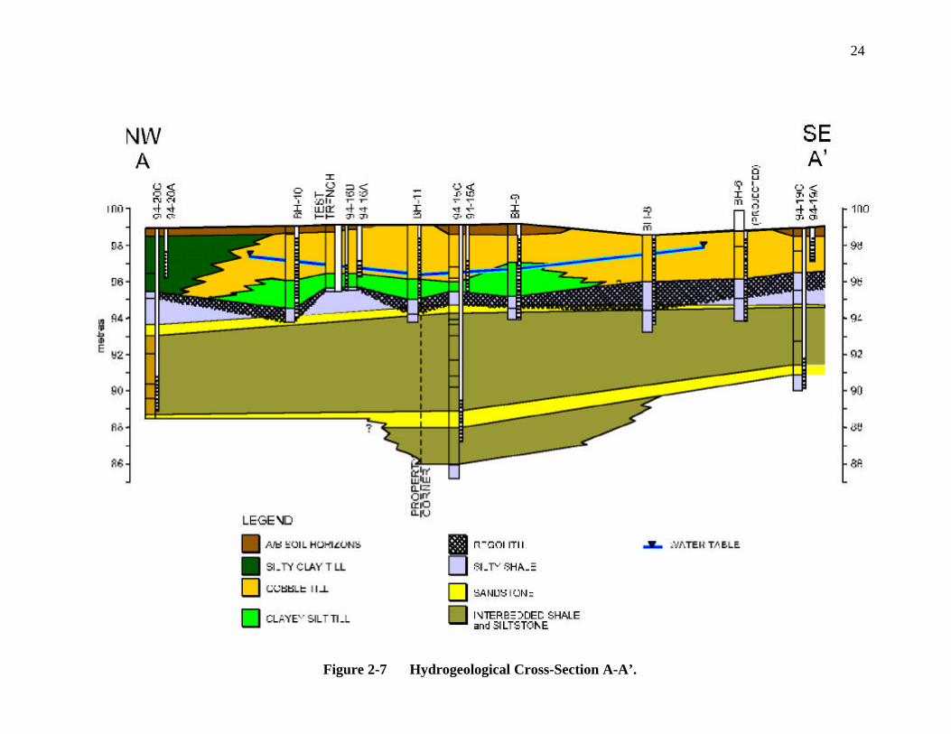
surficial deposits averages approximately 6 m. A hydrogeological cross-section of the
plant, constructed approximately through the area where the Trench and Gate system was
installed, is presented as Figure 2-7. The location of the Trench and Gate installation and
the cross-section transect is shown in plan view on Figure 2-5.

23
Figure 2-6 Electromagnetic (EM-38) Map of the Northeast Corner of the EastGarrington Site.
2.4 GROUNDWATER MONITORING NETWORK
A total of 32 piezometers have been installed at the East Garrington site, including three
wells completed in bedrock. All piezometers completed by O'Connor Associates (1992)
are designated with a BH- prefix and installed in till. Piezometers completed by Komex
International Ltd. are identified with A or B suffixes if installed in the first or second
groundwater-bearing zones in till, or with a C if installed in bedrock. Other wells or
sampling points are designated by the prefixes: CW (Culvert Well) for sampling points
within the treatment gate; GW (Gallery Well) for wells installed in the reinfiltration
gallery; TW (Trench Well) for wells installed within the trenches; PW (Pumping Well);
and, MW (Monitoring Well) for the monitoring well associated with the pumping well.
24
Figure 2-7 Hydrogeological Cross-Section A-A’.

25
A site map showing the location of piezometers is presented as Figure 2-5. Piezometers
were first installed at the site in 1990 by O’Connor (1991). Subsequent installation
programs were completed by Komex in 1994 and 1996. The purpose of these two
programs was to further delineate groundwater impact discovered by O’Connor and to
refine the understanding of groundwater flow patterns. Piezometers were constructed
according to accepted hydrogeologic practices using bentonite seals to prevent annular
leakage. Borehole logs and piezometer construction details are provided in Appendix I.

26
3. HYDRAULIC CONDUCTIVITY TESTING
Estimation of the bulk hydraulic conductivity (K) of the sediments was an essential first
step in characterizing the site and subsequently in determining the expected flux for the
treatment system. Hydraulic conductivity testing was carried out using several different
methods as described in the following sections. Results from these tests were used to
calculate a bulk hydraulic conductivity.
3.1 LABORATORY TESTS
Hydraulic conductivities were measured in the laboratory using falling head permeameters,
and estimated from effective grain sizes after the method of Hazen (1911). Results from
the permeameter laboratory tests are summarized in Table 3-1.
Table 3-1 Permeameter Hydraulic Conductivity Test Results
Geological Unit Silty Clay Tills Cobble Unit
Minimum K (m/s) 2.1 x 10⁻¹¹ 2.4 x 10 -9
Maximum K (m/s) 2.4 x 10⁻⁹ 2.4 x 10⁻⁹
Median K (m/s) 6.1 x 10 -11 2.4 x 10⁻⁹
Mean K (m/s) 2.2 x 10⁻¹⁰ 2.4 x 10⁻⁹
Standard Deviation 3.1 x 10⁻¹⁰ -
Population (n) 3 1
Permeameter results were considered unacceptable as they were not in keeping with
accepted values for these types of geological media. Lack of agreement was attributed to
the small sample size tested, which failed to provide a representative field scale value.

27
Estimation of hydraulic conductivity from grain size was undertaken using Hazen’s
formula:
K = 102Cd Equation 3-1
where:
• d10 is the effective grain size diameter in centimetres and is defined as
the value where 10% of the particles are finer and 90% coarser by
weight;
• C varies from 100 to 150 cm/s depending on the material; and,
• K is the hydraulic conductivity in cm/s.
Representative samples collected from the site yielded laboratory measured effective grain
sizes of 0.02 and 0.008 cm for the cobble till and silty clay tills respectively. Substituting
these values into the formula and using a value of 100 for C, yields hydraulic
conductivities of 4 x 10⁻⁴ m/s for the cobble unit and 6 x 10⁻⁷ m/s for the till. These
calculated values were more in keeping with expectations and were thus considered a
reasonable first approximation of hydraulic conductivity.
3.2 PIEZOMETER TESTS
Hydraulic conductivity tests were conducted to determine in-situ hydraulic conductivity
values on single piezometers (Freeze and Cherry, 1979). These tests were performed by
measuring the static water level, removing water from the piezometer, and recording the
rise in water level with time during recovery.
Water was removed from the piezometers, using either a bailer or Waterra tubing with an
inertial foot valve, until the piezometer was dry or a significant drawdown was obtained.
At that point, bailing was stopped and recovering groundwater levels were measured at
selected time intervals using a standard hand-held electric water level sounder in the well.

28
Groundwater recovery level measurements and interpretation graphs are provided in
Appendix II. In some cases the rate of groundwater recovery was very slow and, due to
time constraints, groundwater recovery data were collected only for as long as was
practical. In other cases, where a drawdown could not be achieved, piezometers were
arbitrarily assigned a hydraulic conductivity of >10-5 m/s (Table 1, Appendix III).
For “BH” series wells where borehole completion information was unknown, hydraulic
conductivity calculations were made assuming the borehole diameter was 15 cm and
screen lengths were from the base of the borehole to 1.0 m below ground level.
Water level recovery data were analyzed using the Bouwer-Rice (1976) method for
unconfined aquifers and the Cooper et al. (1967) method for confined aquifers as
described in the AQTESOLV for Windows User’s Guide (Geraghty & Miller, Inc.,
1996).
Hydraulic conductivity estimates obtained using these methods are approximate due to the
relatively small volume of water removed from the wellbore. Consequently, they are only
representative of the zone within the immediate vicinity of the screened interval. Small
variations in grain size and texture, or fracture density and aperture size, can greatly affect
hydraulic conductivity values within zones of similar lithology. Therefore, these methods
provides only an indication of the order of magnitude of the hydraulic conductivity.
In general, the part of the displacement curve that showed the greatest rate response was
chosen as the basis of the K estimate, resulting in conservative (greater) values. However,
the difference between conservative and non-conservative results rarely exceeded half an
order of magnitude. During the initial phases of a K test, sand pack drainage may
contribute water to the piezometer, resulting in an initial rapid rate of response. The data
were qualitatively analyzed to ensure that the part of the curve chosen for the K estimate
was not significantly influenced by sand pack drainage.

29
For confined aquifer test analyses (94-15C, 94-19C, and 94-20C), the results are
presented as K derived from transmissivity (T). The T result was divided by the thickness
(b) of the groundwater-bearing zone, as inferred from the borehole log, to obtain a value
for K. Based on observations made during drilling, shale units are expected to have very
low permeabilities and were accordingly assigned a hydraulic conductivity of < 1.0 x 10⁻⁹
m/s.
Hydraulic conductivity tests results varied considerably across the site. A summary of
values and statistics for the various units is provided in Table 3-2.
Table 3-2 Summary of Drawdown-Derived Hydraulic Conductivities
Hydrogeological
Unit
Maximum K
(m/s)
Minimum K
(m/s)
Mean K
(m/s)
Median K
(m/s)
StandardDeviation
Population
(n)
Clayey Silt Till 1.7 x 10⁻⁵ 9.9 x 10⁻⁹ 2.9 x 10⁻⁶ 9.0 x 10⁻⁸ 6.0 x 10⁻⁶ 8
Silty Clay Till 5.3 x 10⁻⁷ 5.6 x 10⁻¹⁰ 1.4 x 10⁻⁷ 1.3 x 10⁻⁷ 1.6 x 10⁻⁷ 11
Cobble Till 3.3 x 10⁻⁶ 2.5 x 10⁻⁹ 5.6 x 10⁻⁷ 8.9 x 10⁻⁸ 9.9 x 10⁻⁷ 11
Bedrock 5.2 x 10⁻⁵ 4.7 x 10⁻⁸ 2.1 x 10⁻⁵ 1.1 x 10⁻⁵ 2.7 x 10⁻⁵ 3
Inspection of the table reveals that there are a wide range of hydraulic conductivity values
for each unit. This likely reflects site heterogeneity and the variable contribution of
fractures and sand lenses to permeability.
3.3 EXPERIMENTAL TRENCH HYDRAULIC CONDUCTIVITY TESTING
3.3.1 Test Design
Given the wide range of values from the above tests, and since the results for the tests
represent very local conditions only, a trench pumping test was designed to test a larger

30
volume over a longer time. The test trench was completed in the area where the
remediation system was to be installed adjacent to piezometer nest 16 (Figure 2-5).
Unfortunately, the trench pumping test had to be conducted during the winter of 1995 in
preparation for designing the Trench and Gate system which was to be installed during the
approaching field season. During the winter months the water table dropped below the
cobble-rich till into the underlying clayey silt till. As a result, the hydraulic conductivity of
the more permeable unit could not be determined.
Design parameters for the trench pumping test were initially determined using a drawdown
test. Groundwater was pumped out of the trench rapidly using a submersible pump
installed in Pumping Well 1 (PW-1) and the trench was left to recover. Water levels in the
trench (MW-1) and nearby monitoring wells (16B) were recorded using pressure
transducers and data loggers. The layout of the trench and piezometers is shown in Figure
3-1 and a schematic of the drawdown within the trench and adjacent piezometers is
presented as Figure 3-2. The initial results, which showed a 70% recovery in the trench
over a four day period, were evaluated and used to determine the optimum pumping
parameters for a second constant head drawdown test.
Figure 3-1 Schematic of Trench Pumping Test Layout.

31
Figure 3-2 Drawdown Within the Trench and Piezometers During the TrenchPumping Test.
During the second test, the water level in the trench was depressed approximately 0.7 m
below the static level, and an attempt was made to maintain this drawdown for five days
using a displacement pump. The pump was then shut off and the water level in the trench
allowed to recover. Piezometric levels in the trench and nearby monitoring wells were
again recorded using pressure transducers and data loggers. Interpretation of the recovery
data was hampered by:
• not having a second monitoring well closer to the trench as the
drawdown in 16B was limited;
• not pumping out the trench fast enough;
• temporary failure of the pump on the third day;
• imprecise pump flux monitoring; and,
• uncertainty regarding seepage face development or skin effects within
the trench.

32
3.3.2 Test Results
Results of the second pumping test for the monitoring well (MW-1) installed in the trench,
and adjacent piezometer 16B, located 1.8 m away from the edge of the trench, are
presented as Figure 3-3 and Figure 3-4, respectively. Inspection of the graphs reveals that
despite having pumped the trench essentially continuously for five days, only twelve
centimetres of drawdown was induced in the adjacent monitoring well. This is indicative
of the relatively low permeability of clayey silt till overlying the bedrock.
0.0
0.1
0.2
0.3
0.4
0.5
0.6
0.7
0.8
0.9
1.0
14 15 16 17 18 19 20 21 22 23 24 25 26 27 28 29 30 31 01
MARCH 1995
DR
AW
DO
WN
(m
)
PUMP STOPPED
Figure 3-3 Drawdown vs. Time For Monitoring Well MW-1.
0.00
0.02
0.04
0.06
0.08
0.10
0.12
0.14
14 15 16 17 18 19 20 21 22 23 24 25 26 27 28 29 30 31 01
MARCH 1995
DR
AW
DO
WN
(m
)
PUMP STOPPED
Figure 3-4 Drawdown vs. Time for Piezometer 16B.

33
Drawdown data for the trench pumping test were interpreted using a number of graphical
and calculation-based approaches (Bowles and Bentley, 1995). Two of these approaches
use derivations based on Darcy’s (1856) equation to estimate the hydraulic conductivity of
the sediments around the trench and are presented below. The two approaches are based
on a number of simplifying assumptions including:
1. the aquifer being tested is unconfined, as well as being essentially
infinite, homogeneous and isotropic over the area influenced by the
test;
2. prior to the commencement of pumping, the water table is horizontal
over the area influenced by the test;
3. the monitoring well (16B) and the trench, both fully penetrate the entire
thickness of the aquifer;
4. the underlying bedrock contact is impermeable and horizontal; and,
5. well losses are negligible.
Details of the two approaches are described below.
Approach 1
In the first approach, early time recovery data is used to approximate a flow rate into the
trench. Water levels in the trench and piezometer are then used to calculate hydraulic
conductivity. During recovery, flow into the trench (Q) is equal to the rate of change in
the volume of water in the trench. Q may therefore be calculated from trench length,
trench width, the change in the height of the water with respect to time and drainable pore
space in the trench, as follows:
Q = dnh
tlw
∂∂
Equation 3-2
where:
Q = inflow rate (m3/s);

34
nd = drainable porosity (specific yield, unitless);
l = trench length (m);
w = trench width (m); and,
∂∂h
t= the change in head with respect to time in the trench.
The derivative term can be approximated from the slope of the drawdown vs. time curve
in Figure 3-5 as 1.7 x 10⁻⁶ m/s. This slope is taken from the early part of the recovery
data, and hence the corresponding Q is the flow into the trench immediately after the
pump is turned off.
0.0
0.1
0.2
0.3
0.4
0.5
0.6
0.7
0.8
0.9
1.0
14 15 16 17 18 19 20 21 22 23 24 25 26 27 28 29 30 31 01
MARCH 1995
DR
AW
DO
WN
(m
)
dh/dt = 0.0000017 m/sec
Figure 3-5 Drawdown vs. Time for Monitoring Well MW-1.
If Q* is defined as the volumetric flow into the trench, per unit length of trench perimeter,
it can be written as:
Q* = ( )Q
l w2 +Equation 3-3
The Darcy (1856) equation may be applied to flow towards a unit length of trench as:

35
Q Kih Khh
l* = =
∂∂
Equation 3-4
where l is the distance outwards from the trench face and h is the saturated thickness of
the aquifer at distance l. Integrating between l = 0 (trench face), and l = L (piezometer
16B):
Q l K h hh
hL
T
P
* ∂ ∂= ∫∫0
Equation 3-5
gives:
( )Q LK
h hP T* = −2
2 2 Equation 3-6
which may be rewritten as:
( )QK
Lh hP T* = −
22 2 Equation 3-7
where:
K = hydraulic conductivity (m/s);
L = distance between piezometer and trench face (m);
Ph = height (above bedrock) of water inside monitoring piezometer 16B
at the time the pump was shut off (m); and,
Th = height (above bedrock) of water inside the trench at the time the
pump was shut off (m).
This approach assumes that infiltration through each trench face may be treated as if it
were perpendicular flow into an infinitely long trench. As a result, it assumes no
significant flow input from trench corners.
Combining equations 3-2, 3-3, and 3-7 and rearranging to solve for K gives:
K = ( ) ( )dP T
n Llw
l w h h
h
t+ −1
2 2
∂∂
Equation 3-8
Substituting measured and assumed values of:
nd = 0.24 (Domenico and Schwartz, 1990);

36
l = 3.6 m;
w = 0.9 m;
∂∂h
t= 1.7 x 10⁻⁶ m/s;
L = 1.2 m;
Ph = 0.805 m; and,
Th = 0.135 m;
into Equation 3-8 yields a K of 5.6 x 10⁻⁷ m/s, a reasonable value as compared to known
values for similar types of sediments.
Approach 2
The second approach used to estimate K, approximates flux into the trench as steady state
radial flow towards a large diameter well. This approach is based on the assumption that
the system had reached a quasi steady state (i.e., constant drawdown) towards the end of
the pumping portion of the test. The assumption is supported by the observation that
drawdown in piezometer 16B was changing little at the time the pump was shut off (see
Figure 3-4). Since the pumping rate for the test could only be measured manually and
infrequently, a pumping rate has to be inferred. During the late stages of the pumping part
of the test, the drawdown in the trench is constant, and hence the inflow into the trench,
Q, is equal to the pumping rate. If it is assumed that there is only a gradual change in Q
after pumping is stopped, the volume of Q calculated from early time recovery data in
Equation 3-2 may be used as an approximation for the steady state pumping rate.
Taking the Darcy (1856) equation, transposed into cylindrical coordinates, for radial flow
towards a well, at a radius r, where the saturated aquifer thickness is h:
∂∂
h
tEquation 3-9
and integrating between rT (effective radius of well), and rP (radial distance to piezometer):

37
Qr
rK h h
r
r
h
h
T
P
T
P∂π ∂=∫ ∫2 Equation 3-10
gives:
Qln r r K h hP T P T( / ) ( )= −π 2 2 Equation 3-11
which may be re-written as:
K = ( )
( )Qln
h h
P T
P T
r r
π 2 2−Equation 3-12
where:
Q = total volumetric discharge (m3/s);
K = hydraulic conductivity (m/s);
Ph = height (above bedrock) of water inside monitoring piezometer 16B
at the time the pump was shut off (m);
Th = height (above bedrock) of water inside the trench at the time the
pump was shut off (m);
rP = the distance (m) between the centre of the trench (pumping well)
and piezometer 16B (see below); and,
rT = the effective radius (m) of the pumping well (trench).
Since the pumping trench was not circular, rT was approximated by calculating an
equivalent well radius based on a well with a circumference equal to the perimeter around
the trench or
rT = l w+
πEquation 3-13
where l and w are the length and width of the trench, respectively, as previously defined.
L is the distance from the trench face to the monitoring well, as previously defined, and
therefore the radial distance to the piezometer rP is given by
rP = rT + L Equation 3-14

38
Using the previously defined values in Equation 3-12, calculating rT and rP from equations
3-13 and 3-14, and Q from Equation 3-2, yields a K of 4.1 x 10⁻⁷ m/s. This value
compares favourably with the one calculated from Approach 1 and is also considered to be
in keeping with the expected bulk hydraulic conductivity of the till tested during the
trench pumping.
Other data analyses (Bowles and Bentley, 1995) yielded somewhat larger bulk hydraulic
conductivity estimates ranging from 9 x 10⁻⁶ to 6 x 10⁻⁵ m/s. These values were somewhat
greater than expected as compared with other methods of estimation.
Additional attempts might be made to analyze the data using other analytical methods and
numerical flow modelling. No further attempt was made, however, the data obtained from
the test and other methods were considered sufficiently accurate for estimating the
expected flux and designing the Trench and Gate system. At the time of the test, it was
not understood how much greater the hydraulic conductivity of the cobble till was than the
underlying clayey silt till. This resulted in a significant under estimation of the expected
influx of water into the trench during construction (see Section 5.1.3).
3.4 PREDICTING TREATMENT FLUXES FROM BULK HYDRAULIC CONDUCTIVITIES
Estimates of hydraulic conductivity varied depending on the method used but in general,
and as would be expected, estimates increased when large volumes were tested. Using the
largest (worst case) K value as estimated from the trench pumping test, an approximation
of the expected flux (Q) through the Trench and Gate system was made using the
following formula:
Q = KiA Equation 3-15
where:
A = the area (l x h) = 248 m2 is calculated from the length 62 m (linear
distance between two ends of the funnel) multiplied by the saturated
thickness - h (approximately 4 m);

39
i = the average horizontal hydraulic gradient (see Section 5.2) = 0.035;
and,
K = 6.0 x 10⁻⁵ m/s.
This calculation yields a maximum expected flux of 5.2 x 10⁻⁴ m3/s or approximately 31
litres per minute.

40
4. HYDROGEOLOGY
4.1 REGIONAL HYDROGEOLOGY
The regional hydrogeological setting of the plant is shown in Figure 4-1 and the legend for
this map and subsequent cross-sections is included as Figure 4-2. Cross-sections through
the East Garrington area are presented as Figure 4-3 and Figure 4-4 and the cross section
locations are shown on Figure 4-1. The subcropping Paskapoo Formation bedrock in this
area has been assigned an expected yield in the range of 2 to 8 L/s. This is presumably
due to fracture porosity as most of the bedrock is composed of shale with limited matrix
porosity. It is also in general agreement with the yield from the on-site water well used
for domestic supply.
Figure 4-1 Regional Hydrogeological Map Showing Locations of HydrogeologicalCross-Sections (Ozoray and Barnes, 1977).

41
Figure 4-2 Hydrogeological Legend to Accompany Regional HydrogeologicalMaps and Cross-Sections (Ozoray and Barnes, 1977).

42
Figure 4-3 Regional Hydrogeological Cross-Section B-B’(Ozoray and Barnes,1977).
Figure 4-4 Regional Hydrogeological Cross-Section C-C’ (Ozoray and Barnes,1977).

43
Regional groundwater flow directions are towards the north or northeast and vertical
groundwater gradients can be either upwards or downwards, which is presumably
dependent on temporal fluctuations in recharge. Regionally, surficial deposits, especially
those along river valleys, may constitute usable supplies of groundwater, but locally they
do not. In the East Garrington area, Ozoray and Barnes (1977) list the predominant
hydrochemical groundwater type as being one where bicarbonate and carbonate make up
more than 60% of the total anions and cations are dominated by calcium and magnesium.
Hydrogeological characteristics of deeper bedrock units were not considered relevant to
this study as they were unlikely to influence local recharge/discharge conditions, be used
as a source of drinking water, or be otherwise relevant to the contamination scenario at
the East Garrington Plant.
4.2 SITE HYDROGEOLOGY
4.2.1 Groundwater Flow
Groundwater flow directions across the site have consistently been toward the northeast
since monitoring was initiated (see Section 6.1.3). Flow within the site is controlled by
the generally gently north-eastward dipping topography. Recharge to the uppermost
groundwater-bearing zone occurs as a result of precipitation on-site and more importantly
via recharge from the wetland southwest of the facility (Figure 2-3). Water levels in the
wetland (referred to as the Reference Rod) were routinely collected with potentiometric
elevations from the piezometers (Appendix, Table 1) to determine gradients across the
site.
Piezometers could not be installed down-gradient of the plant, but topographic elevations
and observations made during periods of high water table elevations suggest that at least a
portion of groundwater flow discharges into the southeast trending surface paleodrainage
channel(s) located just northeast of the site. From there, surface water flow carries it
away towards the southeast. Some, or all, of the groundwater flow may also continue on

44
towards the northeast. Uncertainty regarding flow directions is compounded by the local
interrelation between surface water, groundwater, and the presence of a surface water
divide that appears to run through, or close to, the site (Figure 4-1).
Horizontal gradients are seasonally dependent, steepen during the summer, and vary from
approximately 0.02 to 0.04 for the central part of the facility. They are substantially flatter
in the northeast corner of the facility where the higher K sediments are located. Based on
an average K value for the site of approximately 5.0 x 10⁻⁷ m/s, an average summer
gradient (i) of 0.035 and an expected effective porosity (ne) of 0.2 (DeMarsily, 1986) the
average linear groundwater flow velocity (v) for the site as calculated from the formula:
v = Ki Equation 4-1ne
is 8.7 x 10⁻⁸ m/s or approximately 5 m per year.
4.2.2 Groundwater Type
The major ion water chemistry and mineralization of groundwater samples collected on
site is presented in Table 3 of Appendix III and has been characterized on an expanded
Durov diagram (Figure 4-5).
The seven different groundwater types present on site can be grouped together into three
major classes as detailed below:
1. Ca:HCO3+CO3, Ca-Mg:HCO3+CO3, Ca-Na:HCO3+CO3, and Ca-Mg-
Na:HCO3+CO3. These four hydrochemical types represent background
(i.e., recently recharged) conditions with most groundwaters belonging
to the Ca-Mg:HCO3+CO3 hydrochemical type. This group also
includes the hydrochemical water type of the surface water from the
wetland (Reference Rod) southwest of the facility. This is indirect
evidence to support the assumption that the wetland controls recharge
to the uppermost groundwater-bearing zone in the facility.

Figure 4-5 Expanded Durov Diagram.
45

46
2. Na:HCO3+CO3 and Na-Ca-Mg: HCO3+CO3. These groundwater types
represent bedrock conditions in the shallow bedrock piezometers and
the facility water well. The predominance of the Na cation is due to
natural softening of the groundwater.
3. Ca-Mg-Cl:HCO3+CO3. Unlike the other water types present on the
property, this hydrochemical type contains appreciable chloride ion
concentrations indicative of contamination by produced water. Only
three piezometers (96-23A, MW-1, and PW-1) yield groundwater
belonging to this hydrochemical type.
It is noteworthy that piezometers MW-1 and PW-1 show elevated chloride concentrations
as compared to 94-16A and 94-16B which are located just a few metres distant. This
observation suggests that excavation and replacement by higher permeability material
and/or pumping of the test trench produced a preferential pathway for the transport of
chloride enriched water. These two wells are also located closer to the bull's eye of an
electromagnetic high delineated during the geophysical survey (Figure 2-6).
4.3 CONTAMINANT HYDROGEOLOGY
4.3.1 Contaminant Sources, Types, and Distribution
Four major sources of groundwater contamination have been identified at the plant (Figure
2-5). These include:
1. product spills in the tank farm;
2. condensate and produced water overflows from the underground water
storage tank area;
3. overflows from an underground storage tank containing used
lubricating oil; and,

47
4. dissolved phase hydrocarbons leaching from an abandoned flare pit and
pond.
Measurable LNAPL accumulations, which generally do not exceed one centimetre in
thickness, are only present in monitoring wells immediately adjacent to the tank farm (BH-
3, -4, and -5) and the underground lubricating oil storage tank (BH-12).
The highest concentrations of dissolved phase hydrocarbons (Appendix III, Table 4) have
been measured in piezometer BH-7 (10 mg/L total BTEX) and piezometer BH-4 which
yielded volatile (C6 to C11) and semi-volatile (C12 to C22) total purgeable hydrocarbon
concentrations of 11 and 187 mg/L, respectively. However, the result from piezometer
BH-4 represents a single condensate spill and is not representative of the usual conditions.
Based on data collected, it appears that at least two distinct plumes are present in the
northeast corner of the site. The first plume originates from the underground water
storage tank and eastward flowing surface spills. The plume manifests itself as high
dissolved hydrocarbon concentrations in piezometers BH-6, BH-7, and possibly 96-26A.
Interestingly, there is only one historical BTEX detection in piezometer BH-8 where the
plume would be expected. The infrequent detections may be attributed to the location of
BH-8 in a local depression focused recharge centre where surface water frequently
accumulates. This centre possibly recharges the well with fresh unimpacted water.
The second plume appears to be migrating from the abandoned flare pit and areas of
associated soil contamination. This is most obvious in the dissolved hydrocarbon results
from piezometer 96-23A. Other sources such as the tank farm may also be contributing to
this latter plume, but there is insufficient data to quantify the potential input. Cyclical
temporal variations in dissolved hydrocarbon content, thought to be associated with
seasonal changes in water table variations, are not evident in the long term data. The

48
apparently random variation in BTEX content is therefore attributed to contaminant
transport by pulses, possibly caused by precipitation events.
4.3.2 Contaminant Behaviour in Groundwater
Contaminants of concern at the East Garrington site are primarily hydrocarbons. The
mobility of these contaminants is dependent on the hydrogeologic environment and the
physiochemical characteristics of the hydrocarbons. Monocyclic aromatic compounds
such as benzene, toluene, ethylbenzene, and o-, m-, p-xylenes (BTEX) are among the
most water soluble compounds found in petroleum products such as condensate. In areas
of free product accumulation, some of the hydrocarbons will be dissolved into the aqueous
phase according to their respective partitioning coefficients. Aqueous solubilities of
specific compounds will vary with temperature, ionic strength, the presence of other
hydrocarbons and the amount of organic carbon in bedrock. BTEX solubilities as well as
other physical and chemical properties are provided in Table 4-1.
Table 4-1 Physical and Chemical Properties of BTEX Compounds
Compound Formula FormulaWeight(g/mol)
Specific Density(20/4°C)
VapourPressure(mm Hg @ 20-25°C)
WaterSolubility
(mg/L at 20-25°C)
logKow
logKoc
Henry’sLaw
Constant(unitless)
Benzene C6H6 78.11 0.877 76 1,780 2.1 1.9 0.224Toluene C7H8 92.14 0.867 22 515 2.6 2.1 0.274Ethyl-benzene
C8H10 106.17 0.867 7 152 3.1 2.2 0.270
Xylenes C8H10 106.17 ≈0.880 ≈8 ≈180 ≈3 ≈2 0.245
From Montgomery and Welkom (1989).
As a result of the processes of advection, dispersion, diffusion, and retardation,
contaminants will move at different rates. Physical and chemical data illustrate that,
benzene will be less retarded than other BTEX compounds in equivalent hydrogeologic
environments. Because it will be transported the greatest distance, and is a known human

49
carcinogen, benzene is considered the most appropriate indicator of hydrocarbon
contamination for this study. Condensate from the East Garrington plant contains a large
proportion of benzene, thus confirming its suitability. Finally, it appears particularly
appropriate as sampling down-gradient of contaminant sources yields significant benzene
concentrations.
Attenuation of dissolved hydrocarbons can occur by destructive or non-destructive
processes (Buscheck et al., 1996). Non destructive attenuation mechanisms include
dispersion, diffusion, dilution by recharge, and sorption. Destructive attenuation
mechanisms include chemical and biological mass loss processes. The latter is considered
an effective remediation tool. At the East Garrington site, attenuation via biodegradation
was deemed particularly attractive because of its simplicity and the limited need for
artificial intervention.
Under aerobic conditions, unacclimated aqueous biodegradation half lives for benzene
have been estimated to range between 5 and 16 days. However, under unacclimated
anaerobic conditions, estimated half-lives range from 16 weeks to 24 months (Howard et
al., 1991). The rapid biodegradation rate for benzene and other hydrocarbons under
aerobic conditions was why biosparging was chosen as the optimum remediation
technology for use in the gates.
Aerobic biodegradation at the East Garrington site is assumed to occur under the
generalized formula for the degradation of benzene as presented below.
AEROBICBIODEGRATION
C6H6 + 7.5 02 → 6CO2 + 3H2OBenzene + Dissolved → Carbon + Water Oxygen Dioxide
bacteria

50
5. TRENCH AND GATE
5.1 HYDRAULICS AND DESIGN
5.1.1 Theory and Conceptual Design
Modification of the Funnel and Gate system to create the Trench and Gate system, is
based on the concept of focusing groundwater flow through media of comparatively
higher hydraulic conductivity (Bowles et al., 1995 and Bowles et al., 1997). Just as
groundwater flow through a highly permeable lens of sand can be significantly more than
in a surrounding clayey till (Figure 5-1), so, too, can the trench and infiltration gallery
focus flow in the Trench and Gate system. Thus, the Funnel and Gate system was
redesigned to take advantage of this fundamental principle.
Figure 5-1 Effect of High Permeability Zone on Groundwater Flow(after Bear, 1979).
A schematic of the original concept for the Trench and Gate system is provided as Figure
5-2. The Trench and Gate system was designed as an in-situ method for treating
hydrocarbon contaminated groundwater in low hydraulic conductivity glacial sediments.
The system is composed of a cut-off trench excavated in till. The original design called for
anchoring the trench into shallow, relatively impermeable bedrock or other suitably
impermeable material, such as deeper unweathered and unfractured tills. The down-
gradient side, the top, and the base of the trench are sealed with a synthetic liner, and the

51
trench is backfilled with a layered, highly permeable aggregate (gravel or drain rock). The
aggregate is required to encourage drainage and prevent groundwater mounding along the
walls of the trench. Slotted PVC is added to the trench to act as a preferential flow path
to reduce fluid potential losses due to friction and tortuosity. Two such trenches are
constructed at an angle to each other and hydraulically down-gradient of the
contamination.
Figure 5-2 Schematic of Trench and Gate Design.
At the intersection of the trenches, natural gradients channel contaminated groundwater
through a permeable wall or treatment gate. In the gate, air is sparged into the
contaminated groundwater. This promotes natural hydrocarbon biodegradation.
Infrastructure to deliver nutrients, other remediating fluids (e.g., acids or bases), or
solutions to prevent biofouling are also installed during construction. The gate is of a
modular design to facilitate repairs or changes, and can be modified to treat different kinds
of contaminants. Following treatment, the groundwater flows back into the till through an

52
infiltration gallery. The infiltration gallery design is purposely generous in terms of
contact area with the till. This is for two reasons:
1. to facilitate re-infiltration of the groundwater, thus preventing
mounding on the down-gradient side; and,
2. in case the treated water is no longer compatible with the untreated
water causing precipitation of minerals and a concomitant reduction in
effective porosity.
Monitoring wells are installed up-gradient, down-gradient, and along the trench to
measure hydraulic head changes due to the interception system, and to enable
hydrochemical monitoring of degradation of dissolved phase hydrocarbons.
Monitoring of groundwater levels and construction of groundwater flow maps, as well as
computer modelling, has shown that, unlike the Funnel and Gate systems, the capture zone
for Trench and Gate systems is as wide as, or wider than, the width of the funnel between
the up-gradient ends of the trench walls. Additionally, the high hydraulic conductivity
trench appears to focus groundwater flow upwards. This prevents contaminant plumes
from descending below the trench walls, and allows the system to be used in a hanging
curtain configuration. Thus the Trench and Gate system effectively ‘pulls’ flow inwards
rather than simply trying to force flow inwards as in the Funnel and Gate system.
Prior research into the flow fields surrounding Funnel and Gate systems revealed that
significant portions of flow moved around the outside of the funnel walls (Fitts, 1997). A
schematic comparison of flow fields for the Trench and Gate and Funnel and Gate systems
in both areal and cross-sectional orientations is presented as Figure 5-3 and Figure 5-4,
respectively.

53
Figure 5-3 Plan View Schematic Comparison of Flow Lines and Capture Zonesfor the Funnel and Gate and Trench and Gate Systems.
Figure 5-4 Cross-Section Schematic Comparison of Flow Lines and CaptureZones for the Funnel and Gate and Trench and Gate Systems.

54
5.1.2 Engineering Design
The East Garrington Trench and Gate system was designed based on site characterization
and engineering/cost limitations. Collection trenches generally follow the conceptual
design. They are 5 m deep, excavated to bedrock and lined with a reinforced arctic grade
geosynthetic on the down-gradient side. However, because of the unstable slope
conditions slit trenches could not be used and the top portion of the trench had to be
sloped back A schematic cross-section of the way the trench was actually completed is
shown in Figure 5-5. The trench is backfilled with screened gravel and instrumented with
PVC monitoring wells.
Figure 5-5 Schematic Cross-Section of Trench Construction Details.
Monitoring wells are constructed in an “L” shape with a long foot extending down the
trench (Figure 5-6). The horizontal section of the “L," as well as the vertical portion
below and slightly above the water table, is constructed of slotted PVC and connected to a
solid riser pipe running to surface. These monitoring wells (labelled TW for Trench
Wells) are installed approximately every 15 m along the trench (see Figure 2-5), and are
capped at the down-gradient end of the foot. The wells were designed to serve a dual
purpose. Their primary purpose is to serve as monitoring wells. Their secondary purpose,
and the reason for their “L” shape and position near the water table, is to act as conduits
to inject remediating or other fluids. Prior to construction, it was unknown whether there
might be problems with biofouling or mineral precipitation within the trenches. So the “L”

55
shaped wells were added as a provision for injecting and distributing along the length of
the trench a biocide, acid, or other type of fluid. To date, no such action has proved
necessary.
Figure 5-6 Schematic of “L” Shaped Monitoring Well Arrangement.
Underlying these monitoring wells is a continuous length of larger diameter, slotted PVC
pipe flanged to the opening in the first gate. These pipes were designed with a large
diameter to facilitate clean-outs if they become necessary, and also have risers located near
the end of the trench so they too can serve as monitoring wells (Figure 5-6). However,
their primary function is to act as a submerged tile drainage system. Groundwater
entering the trench preferentially flows along the PVC pipe to the treatment gate, thus
reducing fluid potential losses due to friction and tortuosity. Such losses are of particular
concern at this site because the low gradient within the small pilot system produces a
minimal (i.e., <2 cm) head drop along the trench arms. Excessive fluid potential losses
could result in stagnation of the water within the Trench and Gate system when a back
pressure develops as a result of aeration in the gate.

56
Original plans called for construction of a permeable wall treatment system. This design
was discarded in favour of a gate design due to easier field construction and suitability for
long term maintenance. The gate residence time was calculated based on the expected flux
and volume of the gates to ensure that there was sufficient time for groundwater within
the gates to be fully oxygenated and to allow for at least partial biodegradation of
dissolved petroleum hydrocarbons.
Using a calculated volume for three culverts that make up the trench gates of 31.52 m3
(from πr2h where r = 0.91 and h is assumed to be 4 m) and an expected flux of 5.2 x 10⁻⁴
m3/s (see Section 3.4), yields a minimum residence time for water passing through the
system of 16.8 hours, assuming no short-circuiting of flow paths. This figure was deemed
adequate for treatment as a worst case scenario. The use of three in-series culverts was
deemed preferable to using one large culvert, or a permeable wall, as it is ideal for the
completion of field experiments (see Section 5.2.2) and allows for measurement of
concentrations before and after treatment. Incorporation of a divider within the second
culvert provides a method for monitoring of experimental (treated) and control (untreated)
streams. Having three in-series gates also proves more economical in terms of made-to-
order culvert costs and allows for isolation of the gates, or sections of the gates, using
keystone valves. Additionally, culverts can be filled with a substrate or growth medium
for hydrocarbon-degrading bacteria.
The gate is constructed of three 1.8 m diameter by 6 m high cylindrical culverts set
vertically into a cement base (Figure 5-7). Drawings of the piping and civil engineering
details (Drawings 1 and 2 respectively) are included in the pocket. The culverts are
connected to the large diameter PVC pipe in the trench arms, each other, and the
infiltration gallery via a series of welded steel pipes and flanges. Pipes connecting the
culverts are equipped with valves so that flow can be shut off and the culverts pumped out
should repairs or the installation of additional infrastructure become necessary. Two flow
meters are installed in the first culvert to measure the flux from each trench arm. The first

57
culvert also contains the biosparging component, a spiralled micro-pore hose attached to a
galvanized base that keeps it anchored to the floor of the first culvert. Air injected into the
hose produces fine bubbles. Bubbling serves both as an aeration and mixing mechanism.
Air for biosparging is obtained from the instrument air compressor at the gas plant. The
system is designed such that if simple aeration resulting in oxygenation of the groundwater
and biodegradation of hydrocarbons is insufficient for remediation purposes, the pressure
can be increased and volatiles can be removed by sparging. Off-gasses would then be run
into the nearby flare stack if necessary.
Figure 5-7 Plan View of Culvert Arrangement.
From the first culvert, oxygenated water flows through two pipes into the second culvert,
which is divided down the middle. The dual compartment culvert is designed for
experiments involving either two different treatment streams or comparisons between
treated and untreated streams. Water from the second culvert flows through additional
piping into a third culvert where it is again allowed to mix and, if necessary, treated prior
to release. Sample ports (labelled with the prefix CW) connected to surface via PVC
tubing and instrumented with Waterra sampling systems are built into each of the inlet or
outlet pipes in every culvert, allowing for sequential sampling during treatment (Figure 5-
7). The culverts are sealed with fibreglass lids with built-in manholes to allow easy access
to sampling ports.

58
Treated water flows out of the last culvert into an infiltration gallery. The gallery is
composed of a finger arrangement of slit trenches excavated into the glacial sediments and
backfilled with washed gravel. At the end of each finger, monitoring wells are constructed
in the backfill material to allow for on-going hydrochemical and hydraulic monitoring of
the system. Arrangement of the gallery fingers (Figure 5-8) had to be altered from an
idealized fan arrangement (Figure 5-2) due to the presence of an underground pipeline.
Figure 5-8 Infiltration Gallery and Trench Layout.

59
5.1.3 Installation
While digging the trench used for the hydraulic conductivity test, it was observed that the
cobble till unit was very unstable, and that the trench was subject to significant sloughing.
These conditions precluded construction of the pilot system using slit trenches as
originally envisioned, so different construction techniques were evaluated.
The first alternative considered was stabilization of the overburden sediments by freezing,
using cryogenic technology developed for the oil and gas industry. The plan was to
excavate a shallow trench into the sediments which would then be frozen by recirculating
liquid nitrogen through the trench. Following freezing and propagation away from the
trench of a frost field, the sediments would likely stand up to trenching using vertical
walls. This alternative was discarded, being both prohibitively expensive, and not
guaranteed to work. Instead, a standardized construction technique involving the
excavation of a sloped trench was undertaken.
When excavation was attempted in August 1995, it was discovered that high levels of
precipitation received during the summer had caused a rise of the water table into the
overlying cobble unit. The higher permeability of the cobble unit allowed a much higher
flux of groundwater into the excavation than had been predicted. The large quantity of
groundwater influx prevented completion of the Trench and Gate system at that time as it
necessitated wider trench excavations and an impractical trench de-watering and pumping
effort. As a result, the program was postponed while alternative solutions were sought.
One of the alternative solutions contemplated was replacing the synthetic liners by a
continuous wall of interlocking sheet piling. Down-gradient of this wall, a temporary
sheet piling enclosure was to have been used for gate construction. Completion of the
gates would have been followed by perforation of the sheet piling wall to allow
groundwater entry into the culverts. The temporary enclosure was then to be removed.
This would have been followed by excavating along the front (up-gradient side) of the

60
sheet piling and backfilling with drain rock. In this scenario, the up-gradient trench would
not have been excavated down to bedrock. Instead, excavating down to a point below the
lowest water table elevation would have been sufficient to provide a conduit for
groundwater flow towards the gate, thus preventing groundwater mounding. This method
also proved to be cost prohibitive, even when preliminary stripping of the overburden
down to the water table was considered as an option to reduce the cost of installing the
sheet piling.
Failing to find a suitable alternative, completion of the Trench and Gate system using
standard construction techniques was chosen. Details of the construction methodologies
and a construction schedule are presented in Appendix IV.
Appraisal of the system following the first year of operation has revealed that future
Trench and Gate installations may have to be modified to prevent groundwater recharge
from occurring directly through the trench arms during precipitation events and the spring
melt-out of the frost wedge. Significant recharge in this manner may cause groundwater
mounding in the trench if the infiltration gallery is incapable of discharging this large and
sudden flux of surface water into the till. This in turn, could lead to the system backing up
and concomitant groundwater flow around the ends of the trench. Infiltration directly
through the trench can be prevented by sealing the top of the trench with a synthetic liner
or a bentonite slurry and mounding fill back over the trenches to compensate for later
consolidation.
Difficulties were also encountered with the impeller flow meters originally installed in the
first culvert. These were either incapable of resolving flux volumes during periods of low
flow or possibly restricted flow through the system. As a result, they were replaced by
Controlotron flow meters capable of being data logged and measuring the low flows.
Installation of the gate separator in the second culvert following system emplacement also

61
proved to be a challenge and future installations requiring a divider should have this
separator installed prior to the system being lowered into the excavation.
5.2 TREATMENT OF CONTAMINATED GROUNDWATER
5.2.1 Isolation and Identification of Hydrocarbon Degrading Bacterial Species
After operating the system for several months, a biological slime was found to be growing
on the walls of the culverts that were used to construct the gate. A slimy froth also began
to accumulate on the surface of the water in the first culvert. Samples of both the water
and the froth in this culvert were collected in sterilized containers and brought to the
laboratory for isolation and identification of possible hydrocarbon degrading bacterial
species. Details of the experimental design, procedures, and materials used for isolating
the bacteria are provided below (Bowles et al., 1997).
Isolation Media
To ensure the isolation of hydrocarbon degrading bacteria, media lacking an intrinsic
carbon source is required. Atlas (1981) stated that the use of agar media has probably
resulted in the “counting of non-hydrocarbon” degraders due to the inclusion of organic
contaminants in agar media. He therefore recommended the use of silica gel as a
solidifying agent when enumerating hydrocarbon degraders.
Dalynn Laboratory Products used the method of Funk and Krulwich (1964) to prepare a
silica based media for this study. Following this method, a standard inorganic nutrient
mixture (Bacto Bushnell-Hass Broth) was incorporated. This mixture was chosen because
of its limited carbon content and because it is recommended for the microbiological
examination of fuels by the Society of Industrial Microbiologists Committee on Microbial
Deterioration of Fuels (Difco, 1994).

62
Experimental and Control Plates
Negative control plates were run to ensure the media was free of metabolizable carbon.
These plates were inoculated using 1 mL of the specimen. The inoculated plates were
placed into a sealed chamber with an open vial containing water.
Positive control plates were used to determine the presence or absence of micro-
organisms in the inoculant water. These plates were prepared identically to the negative
and experimental control plates except they included 1% dextrose. Positive control plates
were inoculated with 1 mL of specimen water and placed into a sealed chamber with an
open vial of water.
The experimental plates used to isolate the hydrocarbon degrading bacteria were also
inoculated with 1 mL of the specimen water and placed into a closed vessel, but with the
addition of a source of carbon vapours (viz., BTEX) and a vial of water. The hydrocarbon
source used was condensate from the East Garrington plant. This condensate is sweet
(i.e., it does not come from an H2S rich source), composed primarily of light end
hydrocarbons and has a relatively high vapour pressure.
Experimental Design
All tests were run in triplicate and were incubated aerobically at room temperature for two
weeks prior to examining growth. Plates were incubated in an inverted position to reduce
condensation on the media surface. To prevent hydrocarbon deterioration of plastic petri-
dishes (and the subsequent diffusion of the plastic materials into the media), the
experimental plates were prepared using glass petri-dishes.
After incubation, the sealed vessels were opened and examined. Growth patterns were
interpreted using Table 5-1. Isolates were delivered to the Alberta Provincial Laboratory
of Health for speciation.

63
Isolation of Hydrocarbon Degraders
Initially, all three plates showed growth (+/+/+). Accordingly, the colonies were re-plated
and re-incubated for two weeks. Examination of the secondary plates yielded the
anticipated (+/+/-) pattern.
Table 5-1 Growth Results Matrix for Bacteria
Experi-mental
PositiveControl
NegativeControl
Interpretation Action
+ + + Media contaminated withmetabolizable carbon.
Re-plate existing growth onsecondary plates and re-incubate atroom temperature for two weeks.
- - - Sample essentially sterile. Re-sample, re-plate, or amplify.- + - Non-hydrocarbon
degraders present.Confirm interpretation on replicates.
+ + - Hydrocarbon degraderspresent.
Conduct speciation on theexperimental plate.
Notes: (+) Denotes growth occurred on the plate; and,(-) Denotes that no growth occurred on the plate.
Rationale for Re-plating and Incubation of the +/+/+ Result
The growth of organisms on the negative control plate indicates that a carbon source was
present during the primary isolation.
Examination of the components used to construct the media indicated that no carbon
source was present in its make-up. The powdered silica gel used (Grade 923, Lot #
96066, Fisher Scientific), which was dissolved using a 7% KOH solution, contains volatile
acid concentrations (as CH3COOH) of < 0.001%. Likewise, the Bacto Bushnell-Hass
media was composed solely of inorganic salts (Difco, 1994).
However, examination of the inoculating water indicated high levels of dissolved
hydrocarbons. It was hypothesized that the transfer of the inoculating water to the
primary plates resulted in the transfer of a metabolizable carbon source. The re-plating of

64
the primary isolates to secondary plates without the corresponding transfer of carbon
contaminated water was needed to prove this hypothesis.
The secondary plates showed the anticipated +/+/- growth pattern indicating that the
carbon contaminant had been removed. Thus, it can be deduced that the isolates on the
secondary experimental plate were using the hydrocarbon vapour as their sole carbon
source.
Identification and Significance of Isolates
The four isolates identified were:
Pseudomonas putida: The ability of P. putida to degrade a variety of
hydrocarbons such as BTEX and phenolics has been well documented
previously (Heald and Jenkins, 1996).
Pseudomonas fluorescens: Cultures of P. fluorescens capable of using
aromatic hydrocarbons as a sole carbon source have been previously
isolated (Marconi et al., 1996).
Stenotrophomonas maltophilia: S. maltophilia has been demonstrated to
degrade hexahydro-1, 3, 5-trinitro-1, 3, 5 triazine (Binks et al., 1995). It
has also previously been isolated as a toluene and xylenes degrader (Su and
Kafkewitz, 1996).
Rhodococcus sp: R. sp. have been characterized with an ability to degrade
a wide variety of PCB isomers (Wang et al., 1995) including bi-, tri-, tetra-
and pentachlorophenols (Masai et al., 1995).

65
5.2.2 Biodegradation and Nutrient Amendment Experiments
Microcosm experiments performed at the University of Waterloo suggested that given an
adequate supply of dissolved oxygen, biodegradation of BTEX compounds at the East
Garrington site was limited by phosphorous and not nitrogen concentrations (Granger,
1997). To test this hypothesis, and to demonstrate that the remediation system could
degrade high concentrations of dissolved hydrocarbons, a one month field trial was
undertaken. The experimental set-up for the field trial is presented in Figure 5-9.
TREATED WATER TOINFILTRATION
GALLERY
AIRSPARGING
NUTRIENTAMENDED
CONTROL
OXYGENADDITION
GROUNDWATER CAPTURED BYNORTHERN TRENCH ARM
INJECTION OFHYDROCARBONS
GROUNDWATER CAPTURED BYEASTERN TRENCH ARM
Figure 5-9 Schematic Diagram of Experimental Gate Treatment System(Granger, 1997).
During the trial, groundwater spiked with condensate was added to existing contaminated
groundwater in the first of the three in-series treatment gates. This increased the total
dissolved BTEX loading from approximately 0.04 to 2.5 mg/L. Groundwater was aerated
in the first gate by sparging with pure oxygen, instead of atmospheric air (21% O2), to

66
ensure that dissolved oxygen concentration was not a limiting factor for biodegradation.
Following sparging, the water was divided into two separate streams and allowed to flow
through into the second gate. The control stream was left untreated while the second
stream was amended by the addition of nitrogen and phosphorous. Nitrogen was added to
the system by diffusion through low density polyethylene emitter tubes filled with pure
gaseous anhydrous ammonia. Phosphorus was added as a solid in the form of crushed
apatite and powdered commercial fertilizer. These two solids, chosen to provide both
slow and rapid release phosphorous sources, were mixed together and poured into a
slotted PVC well screen which was installed inside the second gate. A schematic
representation of the nutrient amendment infrastructure as installed in the gate is shown in
Figure 5-10.
LDPE-2 EMITTER TUBECONTAININGGROUNDWATER
WELL SCREENCONTAINING FILTER
SAND
LDPE-2 EMITTER TUBECONTAINING AMMONIAGASSTAINLESS STEEL
SUPPORTPARTITION TO CREATEDUAL STREAMTREATMENT CELL
WELL SCREENCONTAINING MIXED
PHOSPHORUS SOURCE
EFFLUENT TOTHIRD GATE
NUTRIENTAMENDED
CONTROL
INFLUENT FROMFIRST GATE
Figure 5-10 Plan View of Nutrient Amendment System in the Second Gate(Granger, 1997).
Analysis of effluent from the second gate showed that biodegradation of BTEX
compounds occurred much more rapidly in the amended stream than in the control stream
(Granger, 1997). Total BTEX concentrations in the amended stream decreased by at least
an order of magnitude during an estimated residence time of 24 hours, while
concentrations on the central side remained essentially unchanged. When the experiment
was repeated and ammonia was added to the control side as well, the results changed little
- confirming that phosphorus is the limiting nutrient. Any dissolved hydrocarbons
remaining in the third gate were removed by aggressive sparging with air. Effluent

67
nitrogen concentrations measured as NO2+NO3 as N were well below Canadian drinking
water guidelines (Health Canada, 1996). The experiment clearly demonstrated that the
system is capable of rapid, in-situ degradation of dissolved BTEX concentrations typical
of highly contaminated plumes.

68
6. DISCUSSION
6.1 HYDRAULIC EVALUATION
6.1.1 Computer Groundwater Modelling
To confirm that the system would perform as predicted, the flow field around the Trench
and Gate infrastructure was modelled using the University of Waterloo’s FRAC3DVS
program (Therrien and Sudicky, 1994). FRAC3DVS is a three dimensional groundwater
flow and solute transport model that can represent discretely fractured and low
permeability media. The Funnel and Gate system was also modelled to illustrate the
differences in flow fields for the two systems.
Details of the modelling parameters used are provided in Hoyne (in prep.) and Hoyne and
Bentley (1997). They used a simplified two layer hydrostratigraphic model with constant
head boundary (Dirichlet) conditions for the four sides and no flow boundary conditions
for the top and bottom of the model. The top layer, designed to represent an unconfined
groundwater-bearing glacial till, was assigned a hydraulic conductivity of 1.7 x 10⁶ m/s.
Underlying the till is bedrock composed primarily of shale with interbedded sandstones
units. This unit was assumed to have a hydraulic conductivity of 1.0 x 10⁻⁸ m/s. The
gravel in the trenches and the infiltration gallery was assigned a hydraulic conductivity of
1.7 x 10⁻³ m/s. The impermeable barrier was modelled using the cut-off wall parameter in
FRAC3DVS. Treatment zones were modelled as enclosed cut-off walls and the
infiltration gallery is configured as a parallelepiped rather than the actual finger
arrangement.
Figure 6-1 is a plan view of the flow lines in and around the Trench and Gate system and
infiltration gallery as modelled using the above parameters. Groundwater flow direction is
from the southwest (lower left hand corner) towards the northeast (upper right hand
corner). For this simulation, the average linear flow velocity in the till outside of the
trench is 3.3 x 10⁻⁸ m/sec or approximately 1 m/year. Inspection of the figure reveals that

69
groundwater flow is focused towards the high permeability trenches and then along the
trenches and into the treatment zone. Following treatment and discharge into the
infiltration gallery, the flow lines fan out again as the water is reinfiltrated into the till.
Results of the simulation suggest that the flow field around the Trench and Gate will
behave as predicted.
Figure 6-1 Plan View of Flow Field for the Trench and Gate System(Hoyne, in prep.).
As can be interpreted from the configuration of the capture zone, and as shown in Figure
6-2, the Trench and Gate system also has an effect on the contours of the potentiometric

70
surface. The preferential flow path caused by the construction of the Trench and Gate
causes a notable elongation, or pulling, of hydraulic head contours towards the apex of the
funnel. This is balanced by a compression of contours around the ends of the trenches
forming the funnel.
Figure 6-2 Plan View of the Potentiometric Surface and Flow Vectors for theTrench and Gate System (Hoyne, in prep.).
Modelling also confirmed that the Trench and Gate capture zone is wider than the width
of the funnel mouth of the system. Other modelling runs have demonstrated that the
Trench and Gate system works just as well in a hanging curtain configuration as it does
when keyed into bedrock (Hoyne, in prep.). This is because the high permeability gravel
trench focuses flow upwards thus preventing stream lines from short circuiting underneath
the walls. The system also has some utility when installed without the impermeable
barrier. However, while groundwater capture continues when the liner is removed,
diffusion may permit down-gradient movement of contaminants across the trench. A three

71
dimensional representation of the flow field for the Trench and Gate system with an
impermeable barrier is shown in Figure 6-3.
Figure 6-3 Three Dimensional Representation of Flow Field in the Trench andGate System (Hoyne, in prep.).
Modelling has also confirmed that, as suspected, the capture zone for the Funnel and Gate
system is narrower than the funnel width (Figure 6-4). The Funnel and Gate design
essentially constricts flow in the area of the treatment gate and forces streamlines to short
circuit underneath the funnel walls or to flow around the outside of the funnel walls, thus
reducing both the horizontal and vertical extent of the capture zone.

72
Figure 6-4 Plan View of Flow Field for the Funnel and Gate System (Hoyne, inprep.).
6.1.2 Hydraulic Response to Infiltration Events
Long term groundwater level monitoring at the East Garrington site has revealed that
fluctuations in potentiometric surfaces, and hence gradients, are much more significant
than previously suspected.
Inspection of groundwater level data (Appendix III, Table 1) shows that the horizontal
hydraulic gradient across the site is seasonally dependent. During the winter, when there
is no recharge, the gradient decreases and causes groundwater flow in the upper
groundwater-bearing zone to slow considerably.

73
Figure 6-5 shows hydrographs for three piezometers (15A, 17A, and 20A) as well as
rainfall, and temperature records for a one year period. Of note in the figure are the large
increases in groundwater levels that correspond to warming trends in the spring (i.e., snow
melt) and infiltration following precipitation. Variability in magnitude of groundwater
level fluctuations between piezometers is also of interest. For example, the first water
level increase in late March is seen as a moderate increase in piezometers 17A and 20A,
and as a large rise (nearly 1.5 m) in piezometer 15A. Groundwater recharge thus appears
to be spatially variable.
Recharge variability is partially attributed to site heterogeneity, and topographic effects
leading to depression focused recharge. However, the response in piezometer 15A is also
likely in part attributable to the infrastructure of the Trench and Gate system itself.
Depressions formed over the areas of the trenches as a result of settlement probably
enhanced recharge directly into the trench during the spring melt. This effect would also
be magnified by the increased permeability of the trench backfill material. Therefore,
piezometers in the immediate area of the trench would likely have been affected by local
groundwater mounding within the trench. Piezometers in this area are also installed in
naturally more permeable sediments. As a result, it is difficult to distinguish between
recharge due to the trench, and recharge due to the increased permeability of the till.
Hydraulic conductivity measurements for these three piezometers, as calculated from
rising head tests, span more than an order of magnitude ranging from 2.8 x 10⁻⁷ for
piezometer 20A to 1.2 x 10⁻⁸ for piezometer 17A (Appendix III - Table 1). Inspection of
the results shows no direct correlation between hydraulic conductivity and the size of
hydraulic head variations. This suggests that sedimentary heterogeneities and possibly
fracturing in the till, play significant roles in the hydraulic head response of piezometers.
However, piezometer 17A, the least permeable of the three, does show a slightly muted
response to precipitation events as compared to the other two. The muted response could
also be explained by its removed location relative to the trenches.

74
Dec-95 Feb-96 Apr-96 Jun-96 Aug-96 Oct-96Date
96
97
98
96
97
98
96
97
98
0
25
50
Rai
nfa
ll (m
m)
-30
0
30
Air
Tem
p (°
C)
17A
15A
20A
Hyd
rau
lic H
ead
(m
)
Figure 6-5 Hydrographs of Response to Melting and Infiltration Events (Thomas,in prep.).
Regardless of the cause, it is obvious that fluctuations in recharge and hence gradients will
affect the flux through the Trench and Gate system. Since recharge is controlled by

75
precipitation, it follows that there should be a direct correlation between major rainfall
events and flux through the Trench and Gate system. This correlation is illustrated in
Figure 6-6 which shows rainfall measurements in relation to fluxes flowing through the
system as measured by the newly installed Controlotron flow meters.
Figure 6-6 Correlation Between Measured Flow Rates Through the Gate andPrecipitation (Thomas, in prep.).

76
The graph shows not only the delayed reaction to rainfall manifested as increased flow
through the system, but also a significant variability in flow through the system.
Data from pressure transducers in nested pairs of piezometers has also shown that not
only the magnitude, but also the direction, of the vertical hydraulic gradients changes in
response to precipitation (Figure 6-7). Smaller scale variations in hydraulic head in
unconfined piezometers have also been shown to be inversely related to changes in
barometric pressure (Thomas, in prep.).
Figure 6-7 Changes in Vertical Hydraulic Gradient in Response to PrecipitationEvents (Thomas, in prep.).
6.1.3 Calculating Bulk Hydraulic Conductivity from Measured Flux
The measurement of treatment fluxes using the Controlotron flow meters has allowed for
the calculation of a bulk hydraulic conductivity. Using an average flow rate through the
system (Q) of approximately 100 litres per hour (Figure 6-6) then the bulk hydraulic
conductivity of the sediments around the Trench and Gate system can be back-calculated
using the same reasoning presented in Section 3.4. If the length (1) for calculating the
area is assumed to be approximately 10% longer (i.e., 68 m) to reflect the increased size

77
of the capture zone relative to the funnel width, and the height (h = 4 m) and gradient (i =
0.035) are held constant, then substitution into the formula:
K = Q Equation 6-1iA
yields a bulk hydraulic conductivity of 2.9 x 10⁻⁶ m/s or approximately one twentieth of
the maximum expected K based on the worst case approximation.
6.1.4 Field Measurement of Potentiometric Surfaces
In an attempt to confirm the modelling results, a number of piezometers were installed in
and around the Trench and Gate infrastructure to see if the modelled flow field would
match field measurements. Field measured hydraulic head distributions for winter and
summer periods prior to installation of the Trench and Gate system are presented as
Figure 6-8 and Figure 6-9, respectively. Similar contour maps for summer and winter
periods following the installation of the Trench and Gate system are included as Figure 6-
10 and Figure 6-11.
Dec. 20, 1994
Figure 6-8 Pre-Trench and Gate Uppermost Groundwater-Bearing ZonePotentiometric Contours, December, 1994.

78
Jun. 07, 1995
Figure 6-9 Pre-Trench and Gate Uppermost Groundwater-Bearing ZonePotentiometric Contours, June, 1995.
Feb. 05, 1996
Figure 6-10 Post-Trench and Gate Uppermost Groundwater-Bearing ZoneContours, February, 1996.

79
Oct. 21, 1996
Figure 6-11 Post-Trench and Gate Uppermost Groundwater-Bearing ZonePotentiometric Contours, October, 1996.
Inspection of the flow field in these four figures leads to a number of observations:
• horizontal hydraulic gradients as measured during the winter are not as
steep as those measured during the summer;
• perturbations in the water table around piezometers BH-2 and 94-18A
persist through time and season and are tentatively attributed to
surveying errors;
• the water table shows a natural flattening in the area of the Trench and
Gate infrastructure prior to and after installation, reflecting the increased
permeability of the cobble till in this area; and,
• post-installation groundwater surface contours curve inwards toward
the apex of the trenches as predicted in the computer modelling. This

80
effect is particularly noticeable for the October 1996 data when the
water table dropped into the less permeable classical till underlying the
cobble till, thus allowing the system to operate in a manner more in
keeping with the design parameters. This effect would be much more
pronounced, and easier to see, if the contouring software could be
programmed not to run contours through the impermeable trench walls.
If they were made to run around the edges of the trench, as they are
physically constrained to do, they would be compressed at the ends of
the trenches as shown in the modelled scenario represented by
Figure 6-2.
Thus it would appear, that under ideal conditions, the flow field in the area around the
Trench and Gate infrastructure behaves as predicted. Differences between what has been
observed and what was predicted are attributed to:
1. a poorer than expected hydraulic conductivity contrast between the
cobble till and the trench backfill material; and,
2. site heterogeneity.
6.2 HYDROCHEMICAL EVALUATION
6.2.1 Field Procedures and Analytical Techniques
General Approach
Field programs sampling included the following:
1. Measurements of the depth to groundwater surface in all piezometers
and at all sample points.
2. Where applicable, measurement of in-situ pre-purge parameters
dissolved oxygen, redox potential, and sometimes temperature.

81
3. Purging of standing water from each piezometer to allow fresh
groundwater to enter followed by sample collection. Either the
piezometer was purged dry, or the equivalent of two borehole volumes
of standing water was removed prior to sampling.
Field Measurements
Field measurements included the following and were measured as detailed below:
Water Levels: measured from the top of the piezometer PVC casing or other
established point using a Solinist electric water level meter.
Temperature: measured in-situ using a dissolved oxygen meter or measured at surface
using either a petroleum distillate-in-glass thermometer or a pH meter
temperature probe.
pH: measured with a Hanna Instruments HI 8733 meter equipped with an
HI 1230 gel-filled multi-purpose probe and calibrated using buffer
solutions of pH 4 and pH 7.
E.C.: electrical conductivity (temperature corrected) measured with a Hanna
Instruments HI 8733 conductivity meter, calibrated with standard KCl
solution (≈ 1,413 µS/cm @ 25 °C).
D.O.: dissolved oxygen measured in-situ with either a YSI type 50B meter
and YSI type 5739 probe (gold cathode, silver anode) calibrated in
water saturated air or with an Oxyguard Handy MK II Dissolved
Oxygen Meter (silver cathode, zinc anode) calibrated in air. Calibration
of both units includes a correction for altitude.
Eh: redox potential measured in-situ using an Oxyguard Handy pH meter or
at surface using a Hanna Instruments HI 8733 pH meter equipped with
an HI 3430 platinum probe. Redox readings were checked against a
standard ZoBell’s solution.

82
Sampling and Analyses
Groundwater samples were collected using dedicated PVC bailers with check valves used
for volatile sampling or dedicated Waterra tubing equipped with inertial footvalves.
Samples were collected in laboratory supplied bottles rinsed with sample water or in
specially pre-cleaned bottles. If necessary, samples were filled in the field using Waterra
disposable in-line filters and preserved with laboratory supplied preservatives. New
bailing rope (where applicable) and disposable gloves were used at each sampling location
and sampling equipment was thoroughly rinsed with distilled water between sampling
stations to prevent cross contamination. Samples were transported in ice packed coolers
to Maxxam Analytics Inc. (formerly Chemex Labs Alberta Inc.) or Amoco’s Tulsa
analytical facility for analysis. Standard chain of custody procedures were followed.
Analytical results have been entered into the Amoco environmental database (AED) and
original laboratory reports have been retained on file at the Komex office.
Analytical procedures for routine potability constituents {bicarbonate (HCO3-), calcium
(Ca2+), chloride (Cl-), iron (Fe2+), magnesium (Mg2+), manganese (Mn2+), nitrate plus
nitrite nitrogen (NO2- + NO3
- as N), potassium (K+), sodium (Na+), sulphate (SO42-), and
total dissolved solids (TDS)}, dissolved organic carbon (DOC), and dissolved metals/
metalloids followed standard methods for the examination of water as detailed in
Table 6-1.
Analysis for dissolved volatile organic hydrocarbons {benzene, toluene, ethylbenzene,
total xylenes (BTEX), total purgeable hydrocarbons as volatiles (TPH C6-C11) and semi-
volatiles (TPH C12-C22)} was completed by Amoco’s Tulsa analytical services department
using a GC-PID/FID freon extraction method (AMM8015) pioneered by Amoco. The
method is described by Miller and Schmidt (1991) and yields a detection limit of 0.001 per
BTEX component and 1.0 mg/L for volatile and semi-volatile components. Occasionally,
BTEX components were also measured by gas chromatography - mass spectrometry (GC-
MS) methods (USEPA Method 8260) by Maxxam Analytics Inc.. Samples analyzed by

83
this method had an improved detection limit (0.0004 mg/L) and reported xylenes results
represent a sum of the individual xylene components.
Table 6-1 Analytical Methods Summary
Analyte Technique NaquadatCode
MethodDetection
Limit (mg/L)Aluminum3 ICP-MS/AES 13109L 0.001/0.01Barium3 ICP-MS/AES 56101L 0.001/0.01Beryllium3 ICP-MS/AES 04102L 0.0002/0.001Bicarbonate2 Alkalinity 06201L 0.5Boron3 ICP-AES 05107L 0.01Cadmium3 ICP-MS 48102L 0.0002Calcium3 ICP-AES 20311L 0.1Chloride1 Ion Chromatography 17209L 0.5Chromium3 ICP-MS/AES 24052L 0.001/0.002Cobalt3 ICP-MS 27102L 0.0003Copper3 ICP-MS/AES 29105L 0.0002/0.001Dissolved Organic Carbon5 InfraRed 06104L 0.2Iron3 ICP-AES 26104L 0.01Lead3 ICP-MS 82103L 0.0003Lithium3 ICP-AES 03101L 0.001Magnesium3 ICP-AES 12311L 0.01Manganese3 ICP-AES 25104L 0.001Nickel3 ICP-MS/AES 28102L 0.0005/0.005NO2+NO3 as N4 Colorimetric 07110L 0.003/0.03Phosphorous3 ICP-AES ICPPHO 0.1Potassium3 ICP-AES 19111L 0.02Silver3 ICP-MS 47102L 0.0001Sodium3 ICP-AES 11311L 0.01Strontium3 ICP-AES 38101L 0.002Sulphate1 Ion Chromatography 16309L 0.1Titanium3 ICP-AES 22009L 0.001/0.003Total Dissolved Solids6 Gravimetric/Calculation 00201L 1.0Uranium3 ICP-MS 102018L 0.0006Vanadium3 ICP-AES 23102L 0.002Zinc3 ICP-MS/AES 30105L 0.0006/0.001
Reference

84
1. Standard Methods for the Examination of Water and Wastewater, 19th ed., American
Public Health Association, Washington, DC, 1995, Method 4110C.
2. Standard Methods for the Examination of Water and Wastewater, 19th ed., American
Public Health Association, Washington, DC, 1995, Method 2320B.
Methods for Chemical Analysis of Water and Wastes, U.S. Environmental Protection
Agency, EMSL, Cincinnati, OH 45268, March, 1979 (EPA-600/4-79-020), Method
310.1.
3. Methods for Chemical Analysis of Water and Wastes, U.S. Environmental Protection
Agency, EMSL, Cincinnati, OH 45268, March, 1979 (EPA-600/4-79-020), Method
200.7.
4. Standard Methods for the Examination of Water and Wastewater, 19th ed., American
Public Health Association, Washington, DC, 1995, Method 4500-NO3E.
Methods for Chemical Analysis of Water and Wastes, U.S. Environmental Protection
Agency, EMSL, Cincinnati, OH 45268, March, 1979 (EPA-600/4-79-020), Method
353.2.
5. Standard Methods for the Examination of Water and Wastewater, 19th ed., American
Public Health Association, Washington, DC, 1995, Method 505A.
Methods for Chemical Analysis of Water and Wastes, U.S. Environmental Protection
Agency, EMSL, Cincinnati, OH 45268, March, 1979 (EPA-600/4-79-020), Method
415.1.
6. Standard Methods for the Examination of Water and Wastewater, 16th ed., American
Public Health Association, Washington, DC, 1985, Method 209B.
Methods for Chemical Analysis of Water and Wastes, U.S. Environmental Protection
Agency, EMSL, Cincinnati, OH 45268, March, 1979 (EPA-600/4-79-020), Method
160.1.

85
6.2.2 Field Measured Parameters
During the research program, field parameters were measured at regular intervals in
observation wells and within the Trench and Gate system. A discussion of these
measurements is presented below. Results are presented in Table 2 of Appendix III.
Electrical Conductivity
Electrical Conductivity (EC) readings recorded from monitoring wells on site range from
311 (BH-4) to 9300 µS/cm (96-23A). Most readings fall within the range of 800 to 1500
µS/cm. Readings below this range likely reflect dilution by large rainfall recharge events.
Values above this range represent high groundwater chloride concentrations and are
limited to the areas down-gradient of the flare pit and holding pond. High chloride
concentrations presumably resulted from the disposal of produced water to the pit and
pond and are in part identifiable from the electromagnetic survey (Figure 2-6).
pH
Values of pH, with the exception of the plant water well and piezometer 96-23A, span a
range from 6.0 to 8.0, with most readings being around the expected median value of 7.0.
The slightly higher values of approximately 8.5 from the water well reflect the influence of
carbonate from the bedrock. The decrease in pH down-gradient of the flare pit (i.e., 96-
23A) is tentatively attributed to disposal of an acidic process chemical or possibly the
breakdown of organic chemicals such as amines which yield an acidic intermediary
daughter product.
Changes in pH were noted for water flowing through the treatment system. Field
measured pH’s for inputs to the system (CW-1 and CW-2) as compared to system outputs
(CW-7) are presented in Figure 6-12. Inspection of the graph reveals that the pH of the
treated water is marginally but consistently elevated relative to the untreated water.

86
6.40
6.80
7.20
7.60
8.00
96-Jul-24 96-Aug-23 96-Sep-22 96-Oct-22
Date
pH
CW-1 (untreated)
CW-2 (untreated)
CW-7 (treated)
Figure 6-12 Temporal Variation in pH for Culvert Wells 1, 2, and 7.
The change in pH is attributed to oxidation of ferrous iron as evidenced by the
accumulation of an iron precipitate on the walls of the culverts and the depletion of
dissolved iron in samples from the third culvert (see Section 6.2.3). The proposed
reaction is shown below. Transformation of the iron consumes protons (H+) creating a
surplus of OH- thus driving the pH up.
4Fe(aq)2+ + O2 + 4H+ + 12OH- → 4Fe(OH)3 (solid) + 2H2O
Ferrous + Dissolved + Proton + Hydroxide → Ferric Hydroxide (amorphous)Iron Oxygen Ferrihydrite (if crystalline)
Dissolved Oxygen
Dissolved oxygen (DO) values across the site vary with location and temporal recharge
conditions. Background values are typically less than 2.0 mg/L except immediately
following a significant precipitation event where they can be seen to increase.
Contaminated wells typically have negligible or zero DO concentrations as do the influent
concentrations to the first culvert. Biosparging in the remediation system increases these
values to fully saturated with respect to air or approximately 10 to 15 mg/L depending on
temperature, mineralization, and other factors. Elevated dissolved oxygen concentrations

87
persist into the infiltration gallery and results as high as 5.0 mg/L are not only common,
but also provide indirect evidence of flow out of the treatment system. Variations in DO
content within infiltration gallery wells also serve to illustrate how flow directions change
through the year with groundwater discharge preferentially occurring down different
fingers of the infiltration gallery. As can be seen in Table 6-2, near background DO
concentrations in GW-3 and GW-4 at the end of May stand in contrast to the values from
the other two wells, and to values in the same wells earlier in the month. This indicates
that these infiltration gallery arms were receiving little oxygenated groundwater discharge
flow from the Gates at this time but had been earlier.
Table 6-2 Dissolved Oxygen Values (mg/L) in Infiltration Gallery Piezometers
Piezometer
Date GW-1 GW-2 GW-3 GW-4
96-May-16 9.6 5.7 7.2 7.2
96-May-31 7.3 3.3 0.8 0.4
Eh
Redox potential measurements span a broad range from -495 to 324 mV. Background
values are typically in the 100 to 200 mV range while contaminated wells are more often
in the -100 to -200 mV range. Eh values can be partially correlated to DO values,
however, they appear to exhibit less short term variability and are not as easily altered by
recharge. Groundwater Eh values show a concomitant increase with dissolved oxygen
values as groundwater flows through and becomes oxygenated in the treatment system
(Appendix III, Table 2).
6.2.3 Laboratory Analytical Data
Dissolved Hydrocarbons
Dissolved hydrocarbon analyses and dissolved organic carbon (DOC) concentrations,
which serves as a general indicator of organic contamination, are presented in Table 4 of

88
Appendix III. Dissolved hydrocarbon analytical data has been collected since 1992.
While different analytical techniques have been used to assess hydrocarbon concentrations
(see Section 6.2.1) the majority of the samples were submitted for analysis of BTEX
(benzene, toluene, ethylbenzene, and total xylenes), and total purgeable hydrocarbons
(TPH) as volatiles (C6-C11) and semi-volatiles (C12-C22). Accordingly, the following
discussion will be limited to these parameters.
Volatile and semi-volatile TPH detections generally do not exceed a few mg/L and are
limited to piezometers immediately down-gradient of contaminant sources such as the
underground water storage tank, the tank farm, and the flare pit.
BTEX concentrations, which represent the primary hydrocarbons of environmental
concern, are discussed in terms of total BTEX concentrations (i.e., benzene + toluene +
ethylbenzene + total xylenes). However, it should be noted that at most locations the
majority of the total BTEX component is composed of benzene. Therefore, the two terms
can be used essentially interchangeably for the following discussion.
Total BTEX concentrations up to approximately 10 mg/L have been recorded for
piezometer samples taken from down-gradient of the underground water storage tank
(BH-7) and represent the most heavily hydrocarbon contaminated samples on site.
Samples taken from piezometers down-gradient of the tank farm and flare pit yield lower
BTEX concentrations in the 0.1 mg/l range. Thus, analytical data confirms the presence
of multiple dissolved hydrocarbon plumes on site. The capture of the plume sourced from
the underground storage tank by the Trench and Gate system is well illustrated by the
significant increases in hydrocarbon concentrations in TW-7 and a concomitant increase at
CW-1 over time.
In general, dissolved organic carbon concentrations serve as a good indicator of significant
dissolved hydrocarbon concentrations at the East Garrington site. Background DOC

89
values are typically less than approximately 10 mg/L while values over 15 mg/L can
generally be correlated with hydrocarbon contamination. Values between 10 and 15 mg/L
may represent background or contaminated samples. Notable for the DOC results is the
high concentration measured in piezometer 96-23A, which exceeds 3000 mg/L. This is
particularly anomalous because very little of this mass is accounted for by purgeable or
extractable hydrocarbons and thus reflects the large quantities of organic material present
in the flare pit, possibly as organic acids formed as a by-product of biodegradation.
To date, the highest measured total BTEX concentration treated by the system (not
including the period when concentrations were artificially increased for experimental
purposes) has been 0.183 mg/L. In this case, and as with most of the previous data,
BTEX concentrations are reduced to less than the detection limit of 0.001 mg/L before the
groundwater exits the third gate. For the three occasions where BTEX components were
still detectable in the infiltration gallery after treatment (June and July, 1996), these
concentrations were low enough, and dissolved oxygen concentrations were high enough,
that any remaining hydrocarbons would have been degraded over a very short distance and
time.
It appears that the treatment system has been able to degrade all incoming hydrocarbons
despite the fact that bacterial growth is limited to the walls of the culvert. In settings with
higher concentrations of hydrocarbons, it may be necessary to add a stationary growth
medium to increase the surface area available for bacterial growth. While it is likely that
some hydrocarbons are volatilized instead of degraded, this is likely to represent a
relatively small fraction as suggested by the following:
1. Biosparging delivery pressure is kept to a minimum thus keeping
agitation to a minimum.
2. Measurement of off-gasses from the sparging culvert using an organic
vapour analyzer with an effective detection limit of 5 ppm, yield

90
background or near-background concentrations of petroleum
hydrocarbons.
3. Biodegradation experiments (see Section 5.2.2) showed that most
hydrocarbon mass destruction was attributable to biodegradation.
Indicators of Biodegradation
Indicators of contamination (chloride and total BTEX), indicators of biodegradation (i.e.,
terminal electron acceptors NO2 + NO3 as N, manganese, iron, and sulphate), and nutrient
(i.e., phosphorous) concentrations are presented in Table 5 of Appendix III.
Analysis reveals that dissolved Fe and Mn concentrations are highest in piezometer 96-
23A, the well with the highest DOC concentrations. Iron and manganese concentrations
across the site are also generally higher in contaminated wells. Iron is removed from
groundwater during treatment as evidenced by decreasing concentrations in samples taken
from culvert wells CW-1 to CW-7 (Figure 6-13). This is supported by visual observations
made during culvert inspections which confirmed the build-up of an iron precipitate on the
sides of the culverts.
NO2 + NO3 as N concentrations exhibit no obvious depletion in contaminated wells.
Phosphorus concentrations are noticeably low across the site, indirectly supporting the
argument that phosphorous is the limiting nutrient at the East Garrington site.
0.0010.010.1
110
11/1/95 1/31/96 5/2/96 8/1/96 11/1/96
Date
Iron
(m
g/L
)
CW-1 (influent)
CW-2 (influent)
CW-7 (effluent)

91
Figure 6-13 Temporal Variation in Dissolved Iron Concentrations for CulvertWells 1, 2, and 7.
Sulphate concentrations are generally quite low across the site and small differences in
concentrations may be attributed to natural sulphate variability within the tills (Hendry
et al., 1986). However, there is some evidence to indicate a decrease in sulphate
concentrations down-gradient of the flare pit as discussed below.
Very strong sewage-like odours were detected in groundwater from piezometer 96-23A.
In an effort to identify the cause of the odour, a volatile Gas Chromatograph-Mass
Spectrometer open scan analysis of a water sample from this piezometer was conducted.
The analysis yielded a concentration of 200 mg/L ethanethiol or ethyl mercaptan C2H6S
(C2H5SH) as shown below:
H H
H - C - C - S - H
H H
The mercaptan is believed to have resulted from an interaction between a polar organic
such as alcohol and hydrogen sulphide (H2S). Under the anaerobic conditions present in,
and down-gradient of the flare pit, natural sulphate (SO42-) dissolved in the groundwater is
reduced to hydrogen sulphide (H2S) by anaerobic bacteria possibly according to the
following:
SO42- + H2O → H2S + 2.5O2
anaerobic bacteria
The excess O2 is utilized by the bacteria. Decreased concentrations of dissolved sulphate
in piezometers down-gradient of the flare pit tend to support this hypothesis. Following

92
the breakdown of the sulphate by bacteria, the H2S will then react with a polar organic to
form the mercaptan according to the generic formula:
R-X + H2S → R-SH
where R is the carbon parent chain and X is the substituent.
As an example, if we take the organic to be a straight chain aliphatic hydrocarbon or a
compound such as ethanol (CH3CH2OH),
H H
H - C - C - OH
H H
it will react with the hydrogen sulphide according to the following:
CH3CH2OH + H2S → C2H5SH + H2O
or
H H H H H H
H - C - C - OH + S → H - C - C - S - H + O
H H H H H H
On emission to atmosphere (i.e., during groundwater sampling) mercaptans will join
together to form a disulphide (e.g., carbon disulphide) which is even more pungent than a
mercaptan:

93
R - SH + HS - R → R - S - S - R
After passing through the treatment gate and being aerated, aerobic bacteria will cleave
the S atom from the mercaptan molecule. This molecule will then be degraded into CO2
and H2O.
Dissolved Metals
Dissolved metals analyses are presented in Table 6 of Appendix III. Most dissolved metal
concentrations are quite low, as would be expected for a natural groundwater system. In
all but a few cases, concentrations are also well below the Canadian drinking water
guidelines (Health Canada, 1996) for parameters which have defined maximum acceptable
concentrations. A notable exception to this generalization are the results from piezometer
96-23A which are significantly higher than all other samples. The higher concentrations of
metals are at least partially due to a relatively lower pH. However, the high
concentrations of DOC in the well suggest that organo-metallic complexing could also be
a contributing factor (Davis et al., 1994). Another notable exception are zinc values
which appear to be elevated in the culvert wells (CW series). This is most likely due to
dissolution of zinc from the galvanized culvert coating.
Piezometers 25A, 25B, and 26A also yielded some slightly elevated metal concentrations.
The reason for this is not readily apparent.
6.3 PERFORMANCE EVALUATION
Costs for the construction of the basic Trench and Gate groundwater remediation system
were compared to the costs of on-site landfarming or landfilling the same material
(Komex, 1997). Results of the comparison indicate that the difference is significant, and
that the Trench and Gate system can be built for less than half the cost of these routinely
considered alternatives. The resultant savings are more than adequate to cover minimal
annual routine maintenance costs for the system.

94
A long term installation also has the advantage of being able to treat new contamination
without added cost. This assuages worries with regard to incurring additional clean-up
costs for soils contaminated by new spills in the remediated area. However, the Trench
and Gate system does require long term installation in order to be effective as it relies on
natural flushing by groundwater flow to transport contaminants to the treatment zone.

95
7. CONCLUSIONS
Biodegradation experiments have identified a number of indigenous organisms capable of
degrading dissolved hydrocarbons. These experiments also showed that under aerobic
conditions, phosphorus is the limiting nutrient at the East Garrington site.
Research indicates that the flow regime within glacial sediments is significantly more
dynamic than previously suspected. Infiltration and recharge rates can be extremely rapid
and quite variable over small areas as illustrated by large short-term fluctuations in water
table elevations. Variations in hydraulic head, and concomitant changes in horizontal
gradients can change the flux through a cross-sectional area significantly and quickly.
These results illustrate that a thorough characterization and understanding of site
geological heterogeneities will significantly improve the chances of designing a successful
remediation system.
Observations made during the initial period of operation confirm that the Trench and Gate
system offers a viable, long-term remediation system capable of treating contaminated
groundwater plumes hosted by low hydraulic conductivity sediments, and that the system
can be equally well applied at numerous other sites. The system also offers several
advantages in terms of increased vertical and horizontal capture zone size as compared
with the Funnel and Gate system. This is illustrated by both field measurements and
computer modelling results.
The Trench and Gate system is very flexible. Minor modifications to the open gate
arrangement accommodate treatment of multiple contaminant types. The open gate
configuration also facilitates routine maintenance. Additionally, operating expenses are
minimal.
The Trench and Gate system has proved to be economical and effective in removing
hydrocarbons from groundwater, especially as compared with other more traditional

96
remediation methods. It has efficiently prevented off-site migration of contaminants.
Controlled experiments have shown that the system is capable of degrading dissolved
hydrocarbons at concentrations significantly higher than those present at the East
Garrington site.

97
8. REFERENCES
Atlas, R.M., 1981. Microbial Degradation of Petroleum Hydrocarbons: an Environmental
Perspective. Microbial Reviews, Vol. 45, pp.180-209.
Bear, J., 1979. Hydraulics of Groundwater, New York, McGraw-Hill Inc., 569 p.
Binks, Peter. R., S. Nicklin, and N.C. Bruce, 1995. Degradation of Haxahydro-1,3,5-
Trinitro-1,3,5-Triazine (RDX) by Stenotrophomonas Maltophilia. Applied and
Environmental Microbiology, Vol. 61, No. 4, pp.1318-1322.
Bostock, H.S., 1967. Physiographic Regions of Canada. Geological Survey of Canada,
Map 1254A.
Bouwer, H. and R. C. Rice, 1976. A Slug Test for Determining Hydraulic Conductivity
of Unconfined Aquifers with Completely or Partially Penetrating Wells. Water
Resources Research, Vol. 12, pp. 423-428.
Bowles, M., L. Bentley, J. Barker, and J. Rathgeber. 1995. In-situ Remediation of
Hydrocarbon Contaminated Groundwater in low Hydraulic Conductivity Media
Using Trench and Gate Technology. Proceedings of the 5th Annual Symposium on
Groundwater and Soil Remediation. Toronto, Ontario, Canada, October 2-6,
1995.
Bowles, M.W. and L.R. Bentley. 1995. Estimating Hydraulic Conductivity Using a
Trench Pumping Test. Proceedings of the Scientific Meeting of the Canadian
Geophysical Union. Banff, Alberta, Canada, May 22-26, 1995.
Bowles, M., L. Bentley, J. Barker, D. Thomas, D. Granger, and H. Jacobs. 1997. The
East Garrington Trench and Gate Program: It Works. Proceedings of the 6th
Annual Symposium on Groundwater and Soil Remediation. Montreal, Quebec,
Canada, March 18-21, 1997.
Buscheck, T.E., D.C. Wickland, and D.L. Kuehne, 1996. Multiple Lines of Evidence to
Demonstrate Natural Attenuation of Petroleum Hydrocarbons in Proceedings of

98
the 1996 Petroleum Hydrocarbons & Organic Chemicals in Groundwater:
Prevention, Detection, and Remediation, November 13-15, 1996. The Westin
Galleria, Houston, Texas.
Cooper, H.H., J.D. Bredehoft, and I.S. Papadopulos, 1967. Response of a Finite-diameter
Well to an Instantaneous Charge of Water. Water Resources Research, Vol. 3, pp.
263-269.
Darcy, H.P.G., 1856. Les fontaines publiques de la Ville de Dijon: Paris, Victor
Dalmont.
D’Astous, A.Y., W.W. Ruland, J.R.G. Bruce, J.A. Cherry, and R.W. Gillham, 1989.
Fracture effects in the shallow groundwater zone in weathered Sarnia-area clay.
Canadian Geotechnical Journal, Vol. 26, pp. 43-56.
Davis, A., J. H. Kempton, and A. Nicholson, 1994. Groundwater transport of arsenic and
chromium at a historical tannery, Woburn, Massachusetts, U.S.A.. Applied
Geochemistry, Vol. 9, pp. 569-582.
De Marsily, G., 1986. Quantitative hydrogeology, Academic Press, London, p. 440.
Difco Laboratories, 1994. Difco Manual, 10th edition. Detroit: Difco Laboratories.
Domenico, P.A. and F.W. Schwartz, 1990. Physical and Chemical Hydrogeology. John
Wiley & Sons, Toronto, 824 p.
Eaton, A.D., L.S. Clesceri and A.E. Greenbery (eds.), 1995. Standard Methods for the
Examination of Water and Wastewater. American Public Health Association,
American Water Works Association, and Water Environment Federation,
Washington, D.C.
Environment Canada, 1991. Historical Streamflow Summary - Alberta, to 1990. Minister
of Supply and Services, Cat. No. En36-418/1990-3, ISBN 0-662-58803-7.
Government Printer.

99
Fitts, Charles R., 1997. Analytic Modeling of Impermeable and Resistant Barriers.
Ground Water, Vol. 35, No. 2., March-April, 1997. pp. 312-317.
Freeze, R.A. and J.A. Cherry, 1979. Groundwater, Prentice Hall, Inc., New Jersey, 604 p.
Funk, H.B. and T.A. Krulwich, 1964. Preparation of Clear Silica Gels that can be
Streaked. Journal of Bacteriology, Vol. 88, pp. 1200-1201.
Geraghty & Miller, Inc., 1996. AQTESOLV for Windows User’s Guide. Hydrosolve
Inc., Weston, VA.
Glass, D.J. (ed.), 1990. Lexicon of Canadian Stratigraphy, Volume 4 - Western Canada.
Canadian Society of Petroleum Geologists, Calgary, Alberta, ISBN 0-920230-23-
7, McAra, p. 772.
Granger, D.A., 1997. Nutrient Amendment to Enhance Aerobic Biodegradation Within a
Funnel-And-Gate System. Master of Science Project. The University of
Waterloo, Waterloo, Ontario, Canada.
Hazen, A., 1911. Discussion of “Dams on Soil Foundations”, Trans. Amer. Soc. Civil
Engrs., Vol. 73, p. 199.
Hazmacon, 1990a. Unpublished Letter Report to Amoco Canada Petroleum Company Ltd.
on Phase 1 Site Investigation of the East Garrington Facility, November 10, 1990.
Hazmacon, 1990b. Soil Vapour Probe Analysis of East Garrington Site. Unpublished Report
to Amoco Canada Petroleum Company Ltd., December 30, 1990.
Health Canada, 1996. Guidelines for Canadian Drinking Water Quality, Sixth Edition,
Minister of Supply and Services Canada, Ottawa Canada Cat.: H48-10/1996E,
ISBN 0-660-16295-4.
Hendry, M.J., J.A. Cherry, and E.I. Wallick, 1986. Origin and Distribution of Sulfate in a
Fractured Till in Southern Alberta, Canada. Water Resources Research, Vol. 22,
No. 1, pp. 45-61.

100
Harrison, B., E.A. Sudicky, and J.A. Cherry, 1992. Numerical Analysis of Solute
Migration Through Fractured Clayey Deposits Into Underlying Aquifers. Water
Resources Research, Vol. 28, No. 2, pp. 515-526.
Heald, S.C. and R.O. Jenkins, 1996. Expression and substrate specificity of the toluene
dioxygenase of Pseudomonas putida NCIMB 11767. Appl. Microbiol.
Biotechnol., No. 45, pp. 56-62.
Hinchee, Robert E. (ed.), 1994. Air Sparging for Site Remediation, Lewis Publishers,
New York, p. 142.
Howard, P.H., R.S. Boethling, W.F. Jarvis, W.M. Meylan, and E.M. Michalenko, 1991.
Handbook of Environmental Degradation Rates, Lewis Publishers, Inc., Michigan,
725 p.
Hoyne, B., (in prep.). Three Dimensional Flow and Transport of a Trench and Gate
System in a Low Permeability Till, Master of Science thesis, University of Calgary,
Department of Geology and Geophysics, Calgary, Alberta, Canada.
Hoyne, B. and Bentley, L., 1997. Simulating the performance of passive remediation
designs in low permeability tills. Paper presented at the CSPG-SEPM 1997 Joint
Convention, June 1- 6, 1997, Calgary, Alberta, Canada.
Keller, C.K., G. Van Der Kamp, and J.A. Cherry, 1988. Hydrogeology of two
Saskatchewan tills, I. Fractures, bulk permeability, and spatial variability of
downward flow. Journal of Hydrology, Vol. 101, pp. 97-121.
Komex International Ltd., 1993. Spring and Fall 1993 Groundwater monitoring Program at
Amoco East Garrington Gas Plant. Unpublished Letter Report to Amoco Canada
Petroleum Company Ltd. December, 1993.
Komex International Ltd., 1997. The Trench and Gate Remediation System. Unpublished
Report Prepared for the GASReP Research Program, March, 1997.

101
Lord, D., J. Lei, M. Chapdelaine, J. Sansregret, and C. Benoit, 1995. In Situ Air Sparging
for Bioremediation of Groundwater and Soils in In Situ Aeration: Air Sparging,
Bioventing, and Related Remediation Processes, eds. R. Hinchee, R. Miller, Paul
Johnson. Battelle Press, Columbus, Ohio, pp. 121 - 126.
Marconi, Andrea M, F. Beltrametti, G. Bestetti, F. Solinas, M. Ruzzi, E. Galli, and E.
Zennaro, 1996. Cloning and Characterization of Styrene Catabolism Genes from
Pseudomonas fluorescens ST. Applied and Environmental Microbiology, Vol. 62,
No. 1, pp. 121-127.
Masai, Eiji, A. Yamada, J.M. Healy, T. Hatta, K. Kimbara, M. Fukuda, and K. Yano,
1995. Characterization of Biphenyl Catabolic Genes of Gram-Positive
Polychlorinated Biphenyl Degrader Rhodococcus sp. Strain RHA1. Applied and
Environmental Microbiology, Vol. 61, No. 6, pp. 2079-2085.
McKay, L.D., R.W. Gillham, and J.A. Cherry, 1993a. Field experiments in a fractured
clay till. 1. Hydraulic conductivity and fracture aperture. Water Resources
Research, Vol. 29, No. 4, pp. 1149-1162.
McKay, L.D., R.W. Gillham, and J.A. Cherry, 1993b. Field experiments in a fractured
clay till. 2. Solute and colloid transport. Water Resources Research, Vol. 29, No.
12, pp. 3879-3890.
Miller, T.G. and G.W. Schmidt, 1991. Field-Freon Extraction of Dissolved Hydrocarbons
in Groundwater. Proceedings of the Conference on Petroleum and Organic
Chemicals in Groundwater. American Petroleum Institute / Association of
Groundwater Scientists and Engineers Joint Conference, November 20th to 22nd,
1991, Houston, Texas. Water Well Journal Pub. Co. ISSN 1047-9023, pp. 45-57.
Montgomery and Welkom, 1989. Groundwater Chemicals Desk Reference, Lewis
Publishers, Inc., Michigan, 640 p.

102
O'Connor Associates, 1991. Environmental Assessment, Garrington Gas Plant, 11-17-34-
3-W5M. Unpublished Report prepared for Amoco Canada Petroleum Company
Ltd. March, 1991.
O'Connor Associates, 1992. Environmental Site Monitoring, Amoco East Garrington Gas
Plant, 11-17-34-3-W5M. Unpublished Report to Amoco Canada Petroleum Company
Ltd., October, 1992.
Ozoray, G.F., and R. Barnes, 1977. Hydrogeology of the Calgary-Golden Area, Alberta.
Alberta Research Council Report 77-2, p. 38.
Pankow, J.F., R.L. Johnson, and J.A. Cherry, 1993, Air Sparging in Gate Wells in Cutoff
Walls and Trenches for Control of Plumes of Volatile Organic Compounds
(VOCs). Groundwater Vol. 31, No. 4, July - August, 1993, pp. 654-663.
Rowe, R.K., and J.R. Booker, 1990. Contaminant migration through fractured till into an
underlying aquifer. Canadian Geotechnical Journal, Vol. 27, No. 4, pp. 484-495.
Ruland, W.W., J.A. Cherry, and S. Feenstra, 1991. The depth of fractures and active
ground-water flow in a clayey till plain in Southwestern Ontario. Ground Water,
Vol.29, No. 3, pp. 405-417.
Shetson, I., 1987. Quaternary Geology, Southern Alberta. Alberta Research Council
Map. Scale 1:500,000.
Shikaze, S.G. and C.D. Austrins, 1995. A 3-D Numerical Investigation of Groundwater
Flow in the Vicinity of a Funnel-and-Gate System. Proceedings of the 5th Annual
Symposium on Groundwater and Soil Remediation. Toronto, Ontario, Canada,
October 2-6, 1995.
Snow, D.T., 1968. Rock fracture spacings, openings and porosities. J. Soil Mech. Found.
Div. Am. Soc. Civ. Eng., 94 (SMI), pp. 73-91.
Snow, D. T., 1969. Anisotropic permeability of fractured media. Water Resources
Research, Vol. 5, No. 6, pp. 1273-1289.

103
Starr, R.C., and J.C. Cherry, 1994. In-situ Remediation of Contaminated Ground Water: The
Funnel-and-Gate System. Ground Water, Vol. 32, No. 3, pp. 465-476.
Shikaze, S.G., C.D. Austrins, D.J.A. Smyth, J.A. Cherry, J.F. Barker, and E.A. Sudicky.
1995. The Hydraulics of a Funnel-and-Gate System: A Three-Dimensional Numerical
Analysis. Proceedings of the 5th International Association of Hydrogeologists. June 8-
12. Edmonton, Alberta.
Su, J.J. and D. Kafkewitz. 1996 Toluene and Xylene Degradation by a Denitrifying
Strain of Xanthomonas maltophilia with Limited or no Oxygen. Chemosphere.
Vol. 32, No. 9, pp. 1843-1850.
Therrien, R., and E.A. Sudicky, 1996. Three-dimensional analysis of variably-saturated
flow and solute transport in discretely-fractured porous media. Journal of
Contaminant Hydrology, Vol. 23, pp. 1-44.
Thomas, David, (in prep.). Monitoring and Characterization of Water Fluxes at a Trench
and Gate Groundwater Remediation Site, Master of Science thesis, University of
Calgary, Department of Geology and Geophysics, Calgary, Alberta, Canada.
Wang, Ying, James Garnon, Diane Labbé, Hélène Bergeron, and Peter C.K. Lau, 1995.
Sequence and Expression of the bpdC1C2BADE Genes Involved in the Initial
Steps of Biphenyl/Chlorobiphenyl Degradation by Rhodococcus sp. M5. Gene,
Vol. 164, pp. 117-122.
Weber, J.K. and J.F. Barker, 1994. Field-Scale Remediation of Hydrocarbon
Contaminated Soil and Water Using an In-Situ Funnel-And-Gate Strategy.
Proceedings of the 4th Annual Symposium on Groundwater and Soil Remediation.
Calgary, Alberta, Canada, September 21-23, 1994, pp. 45-49.

104
APPENDIX I
BOREHOLE LOGS
AND
PIEZOMETER CONSTRUCTION DETAILS
(SEE HARD COPY)

140
APPENDIX II
HYDRAULIC CONDUCTIVITY DATA
AND
CALCULATIONS
(FOR GRAPHS, SEE HARD COPY)

HYDRAULIC CONDUCTIVITY TEST
AMOCO CANADAEast Garrington
Piezometer: BH-2
Date 96/06/06Hydraulic Conductivity (m/s) 5.34 x 10⁻⁷
Piezometer Stick-up (m) 0.58Screen Length (m) 3.6Total depth below top of PVC (m) 5.18Static water level (m below top of PVC) 1.9
Observations:
Elapsed Time Water level Drawdown (sec) (m) (m)
30 4.870 2.97060 4.740 2.84090 4.600 2.700120 4.465 2.565150 4.350 2.450180 4.215 2.315240 3.980 2.080300 3.745 1.845450 3.255 1.355600 2.875 0.975750 2.575 0.675900 2.360 0.4601800 2.165 0.2652700 2.145 0.2453600 2.130 0.2305400 2.105 0.2059000 2.080 0.18012300 2.055 0.155

HYDRAULIC CONDUCTIVITY TEST
AMOCO CANADAEast Garrington
Piezometer: BH-6
Date 96/5/31Hydraulic Conductivity (m/s) 1.27 x 10⁻⁷
Piezometer Stick-up (m) 0.65Screen Length (m) 4.9Total depth below top of PVC (m) 6.55Static water level (m below top of PVC) 1.955
Observations:
Elapsed Time Water level Drawdown (sec) (m) (m)
30 5.220 3.26560 5.170 3.21590 5.110 3.155
120 5.055 3.100150 4.995 3.040180 4.955 3.000240 4.845 2.890300 4.735 2.780450 4.455 2.500600 4.165 2.210750 3.885 1.930900 3.610 1.6551800 3.065 1.1102700 2.690 0.7353600 2.310 0.3555400 1.960 0.0059000 1.955 0.000

HYDRAULIC CONDUCTIVITY TESTAMOCO CANADAEast Garrington
Piezometer: BH-8 Piezometer: BH-8
Date 95/05/23 Date 96/5/21Hydraulic Conductivity (m/s) 9.14 x 10⁻⁸ Hydraulic Conductivity (m/s) 1.31 x 10⁻⁷
Piezometer Stick-up (m) 0.77 Piezometer Stick-up (m) 0.77Screen Length (m) 3.9 Screen Length (m) 3.9Total depth below top of PVC (m) 5.67 Total depth below top of PVC (m) 5.67Static water level (m below top of PVC) 1.901 Static water level (m below top of PVC) 1.875
Observations: Observations:
Elapsed Time Water level Drawdown Elapsed Time Water level Drawdown (sec) (m) (m) (sec) (m) (m)15 5.640 3.739 30 5.600 3.72530 5.610 3.709 60 5.550 3.67545 5.585 3.684 90 5.480 3.60560 5.555 3.654 120 5.400 3.52575 5.515 3.614 150 5.345 3.47090 5.495 3.594 180 5.275 3.400
120 5.470 3.569 240 5.160 3.285150 5.440 3.539 300 5.050 3.175180 5.385 3.484 450 4.850 2.975210 5.335 3.434 600 4.585 2.710240 5.230 3.329 750 4.435 2.560300 5.130 3.229 900 4.240 2.365360 5.045 3.144 1800 3.645 1.770420 4.960 3.059 2700 3.345 1.470480 4.880 2.979 3600 3.125 1.250600 4.740 2.839 5400 2.805 0.930900 4.450 2.549 9000 2.430 0.5551200 4.255 2.3541800 3.963 2.0623600 3.440 1.5394680 3.150 1.249

HYDRAULIC CONDUCTIVITY TEST
AMOCO CANADAEast Garrington
Piezometer: BH-9
Date 95/05/23Hydraulic Conductivity (m/s) 8.93 x 10⁻⁸
Piezometer Stick-up (m) 0.80Screen Length (m) 4.3Total depth below top of PVC (m) 6.1Static water level (m below top of PVC) 3.302
Observations:
Elapsed Time Water level Drawdown (sec) (m) (m)
15 5.290 1.98830 5.272 1.97045 5.251 1.94960 5.237 1.93575 5.216 1.91490 5.202 1.900120 5.171 1.869150 5.145 1.843180 5.120 1.818210 5.098 1.796240 5.077 1.775300 5.041 1.739360 5.011 1.709420 4.986 1.684600 4.935 1.633750 4.900 1.5981200 4.880 1.5781800 4.850 1.5482400 4.820 1.5183000 4.795 1.493

HYDRAULIC CONDUCTIVITY TEST
AMOCO CANADAEast Garrington
Piezometer: BH-10
Date 96/06/14Hydraulic Conductivity (m/s) 9.87 x 10⁻⁹
Piezometer Stick-up (m) 0.95Screen Length (m) 4.0Total depth below top of PVC (m) 5.95Static water level (m below top of PVC) 2.96
Observations:
Elapsed Time Water level Drawdown (sec) (m) (m)
30 5.630 2.67560 5.535 2.58090 5.460 2.505120 5.410 2.455150 5.375 2.420180 5.350 2.395240 5.325 2.370300 5.310 2.355450 5.280 2.325600 5.260 2.305750 5.245 2.290900 5.225 2.2701800 5.145 2.1902700 5.090 2.1353600 5.040 2.0852700 4.960 2.0059000 4.820 1.86511100 4.740 1.785

HYDRAULIC CONDUCTIVITY TEST
AMOCO CANADAEast Garrington
Piezometer: BH-11
Date 95/05/23Hydraulic Conductivity (m/s) 1.66 x 10⁻⁷
Piezometer Stick-up (m) 0.91Screen Length (m) 3.3Total depth below top of PVC (m) 5.21Static water level (m below top of PVC) 3.65
Observations:
Elapsed Time Water level Drawdown (sec) (m) (m)
15 5.150 1.50030 5.110 1.46045 5.080 1.43060 5.060 1.41075 5.030 1.38090 5.015 1.365120 4.980 1.330150 4.940 1.290180 4.905 1.255210 4.870 1.220240 4.830 1.180300 4.780 1.130360 4.735 1.085420 4.695 1.045480 4.658 1.008540 4.623 0.973600 4.595 0.945900 4.500 0.8501500 4.436 0.7862100 4.420 0.7703480 4.400 0.7509360 4.350 0.700

HYDRAULIC CONDUCTIVITY TEST
AMOCO CANADAEast Garrington
Piezometer: 94-15A
Date 94/12/20Hydraulic Conductivity (m/s) 2.03 x 10⁻⁸
Piezometer Stick-up (m) 0.65Screen Length (m) 2.5Total depth below top of PVC (m) 4.25Static water level (m below top of PVC) 3.58
Observations:
Elapsed Time Water level Drawdown (sec) (m) (m)
60 4.130 0.55090 4.120 0.540
120 4.114 0.534150 4.110 0.530180 4.108 0.528240 4.102 0.522300 4.098 0.518360 4.097 0.517420 4.093 0.513480 4.092 0.512900 4.082 0.5021740 4.075 0.4955220 4.065 0.4857800 4.064 0.484
10860 4.058 0.47813980 4.055 0.47519500 4.050 0.470

HYDRAULIC CONDUCTIVITY TEST
AMOCO CANADAEast Garrington
Piezometer: 94-15C
Date 94/12/20Hydraulic Conductivity (m/s) 4.67 x 10⁻⁸
Piezometer Stick-up (m) 0.57Screen Length (m) 1.5Total depth below top of PVC (m) 12.17Static water level (m below top of PVC) 2.93
Observations:
Elapsed Time Water level Drawdown (sec) (m) (m)120 11.320 8.390180 11.305 8.375240 11.297 8.367300 11.287 8.357600 11.255 8.3251920 11.150 8.2203120 11.070 8.1406360 10.890 7.9608940 10.735 7.80512300 10.062 7.13215180 9.490 6.56020640 8.500 5.570
T/b = K(4.2x10⁻⁸ m2/sec) / 0.9 m = 4.67x10⁻⁸ m/s

HYDRAULIC CONDUCTIVITY TEST
AMOCO CANADAEast Garrington
Piezometer: 94-16A Piezometer: 94-16A Date 95/06/07 Date 96/7/5Hydraulic Conductivity (m/s) 4.51 x 10⁻⁷ Hydraulic Conductivity (m/s) 9.53 x 10⁻⁷
Piezometer Stick-up (m) 0.54 Piezometer Stick-up (m) 0.54Screen Length (m) 1.5 Screen Length (m) 1.5Total depth below top of PVC (m) 3.36 Total depth below top of PVC (m) 3.345Static water level (m below top of PVC) 3.014 Static water level (m below top of PVC) 2.89 Observations: Observations:
Elapsed Time Water level Drawdown Elapsed Time Water level Drawdown (sec) (m) (m) (sec) (m) (m)
30 3.270 0.256 30 3.135 0.24545 3.250 0.236 60 3.090 0.20060 3.240 0.226 90 3.060 0.17090 3.220 0.206 120 3.035 0.145
120 3.205 0.191 150 3.015 0.125180 3.180 0.166 180 2.995 0.105240 3.160 0.146 240 2.970 0.080300 3.140 0.126 300 2.955 0.065360 3.120 0.106 450 2.925 0.035420 3.105 0.091 600 2.915 0.025480 3.095 0.081 750 2.905 0.015540 3.083 0.069 900 2.900 0.010660 3.067 0.053 1800 2.895 0.005900 3.045 0.031 2700 2.890 0.000
1230 3.027 0.013

HYDRAULIC CONDUCTIVITY TEST
AMOCO CANADAEast Garrington
Piezometer: 94-17A
Date 94/12/20Hydraulic Conductivity (m/s) 1.19 x 10⁻⁸
Piezometer Stick-up (m) 0.58Screen Length (m) 3.0Total depth below top of PVC (m) 4.98Static water level (m below top of PVC) 3.71
Observations:
Elapsed Time Water level Drawdown (sec) (m) (m)
30 4.870 1.16060 4.864 1.154
150 4.860 1.150180 4.857 1.147210 4.852 1.142240 4.849 1.139270 4.847 1.137300 4.843 1.133360 4.839 1.129420 4.835 1.125480 4.832 1.122540 4.829 1.119660 4.820 1.110900 4.814 1.104
1560 4.800 1.0903540 4.785 1.0755520 4.778 1.068
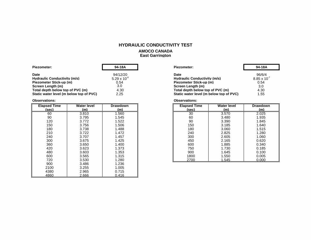
HYDRAULIC CONDUCTIVITY TESTAMOCO CANADAEast Garrington
Piezometer: 94-18A Piezometer: 94-18A
Date 94/12/20 Date 96/6/4Hydraulic Conductivity (m/s) 5.29 x 10⁻⁸ Hydraulic Conductivity (m/s) 8.85 x 10⁻⁷
Piezometer Stick-up (m) 0.54 Piezometer Stick-up (m) 0.54Screen Length (m) 3.0 Screen Length (m) 3.0Total depth below top of PVC (m) 4.30 Total depth below top of PVC (m) 4.30Static water level (m below top of PVC) 2.25 Static water level (m below top of PVC) 1.55
Observations: Observations:
Elapsed Time Water level Drawdown Elapsed Time Water level Drawdown (sec) (m) (m) (sec) (m) (m)
60 3.810 1.560 30 3.570 2.02590 3.795 1.545 60 3.480 1.935
120 3.772 1.522 90 3.390 1.845150 3.756 1.506 150 3.185 1.640180 3.738 1.488 180 3.060 1.515210 3.722 1.472 240 2.825 1.280240 3.707 1.457 300 2.605 1.060300 3.675 1.425 450 2.165 0.620360 3.650 1.400 600 1.885 0.340420 3.623 1.373 750 1.730 0.185480 3.603 1.353 900 1.645 0.100600 3.565 1.315 1800 1.550 0.005720 3.530 1.280 2700 1.545 0.000900 3.486 1.2362100 3.255 1.0054380 2.965 0.7154860 2.666 0.416

HYDRAULIC CONDUCTIVITY TEST
AMOCO CANADAEast Garrington
Piezometer: 94-19A
Date 95/05/23Hydraulic Conductivity (m/s) 3.28 x 10⁻⁶
Piezometer Stick-up (m) -0.06Screen Length (m) 0.98Total depth below top of PVC (m) 1.64Static water level (m below top of PVC) 0.738
Observations:
Elapsed Time Water level Drawdown (sec) (m) (m)
15 1.440 0.70230 1.410 0.67245 1.385 0.64760 1.360 0.62275 1.335 0.59790 1.290 0.552
120 1.245 0.507150 1.170 0.432180 1.110 0.372210 1.060 0.322240 1.005 0.267300 0.922 0.184360 0.854 0.116420 0.808 0.070480 0.780 0.042540 0.763 0.025600 0.760 0.022720 0.755 0.017900 0.754 0.016

HYDRAULIC CONDUCTIVITY TESTAMOCO CANADAEast Garrington
Piezometer: 94-19C Piezometer: 94-19C
Date 94/12/20 Date 95/06/07Hydraulic Conductivity (m/s) 1.95 x 10⁻⁵ Hydraulic Conductivity (m/s) 2.26 x 10⁻⁵
Piezometer Stick-up (m) -0.10 Piezometer Stick-up (m) -0.10Screen Length (m) 1.4 Screen Length (m) 1.4Total depth below top of PVC (m) 8.54 Total depth below top of PVC (m) 8.54Static water level (m below top of PVC) 1.49 Static water level (m below top of PVC) 0.99
Observations: Observations:
Elapsed Time Water level Drawdown Elapsed Time Water level Drawdown (sec) (m) (m) (sec) (m) (m)
60 5.910 4.420 30 5.250 4.26390 5.450 3.960 45 5.020 4.033
120 5.080 3.590 60 4.800 3.813150 4.700 3.210 90 4.410 3.423180 4.345 2.855 120 4.050 3.063210 4.060 2.570 150 3.740 2.753240 3.800 2.310 180 3.440 2.453300 3.330 1.840 210 3.190 2.203360 2.960 1.470 240 2.980 1.993420 2.690 1.200 270 2.770 1.783480 2.460 0.970 300 2.590 1.603600 2.140 0.650 330 2.420 1.433720 1.960 0.470 360 2.300 1.313900 1.800 0.310 390 2.170 1.1831200 1.690 0.200 420 2.050 1.063
450 1.960 0.973T/b = K 480 1.870 0.883(9.78x10⁻⁶ m2/sec) / 0.5 m = 1.95x10⁻⁵ m/s 570 1.670 0.683
600 1.630 0.643900 1.350 0.3631200 1.260 0.273
T/b = K(1.13x10⁻⁵ m2/sec) / 0.5 m = 2.26x10⁻⁵ m/s

HYDRAULIC CONDUCTIVITY TEST
AMOCO CANADAEast Garrington
Piezometer: 94-20A
Date 94/12/20Hydraulic Conductivity (m/s) 2.81 x 10⁻⁷
Piezometer Stick-up (m) 0.54Screen Length (m) 1.0Total depth below top of PVC (m) 3.20Static water level (m below top of PVC) 2.26
Observations:
Elapsed Time Water level Drawdown (sec) (m) (m)
60 2.958 0.69890 2.950 0.690
120 2.935 0.675150 2.922 0.662180 2.912 0.652210 2.898 0.638270 2.878 0.618360 2.843 0.583480 2.803 0.543660 2.747 0.487840 2.700 0.440
1080 2.637 0.3771800 2.510 0.2504740 2.320 0.060

HYDRAULIC CONDUCTIVITY TEST
AMOCO CANADAEast Garrington
Piezometer: 94-20C
Date 94/12/20Hydraulic Conductivity (m/s) 5.16 x 10⁻⁵
Piezometer Stick-up (m) 0.52Screen Length (m) 1.4Total depth below top of PVC (m) 10.57Static water level (m below top of PVC) 2.575
Observations:
Elapsed Time Water level Drawdown (sec) (m) (m)
30 3.880 1.30560 3.130 0.55590 2.840 0.265
120 2.735 0.160150 2.705 0.130180 2.690 0.115210 2.685 0.110300 2.672 0.097330 2.670 0.095510 2.665 0.090
T/b = K(5.68x10⁻⁵ m2/sec) / 1.1 m = 5.16x10⁻⁵ m/s

HYDRAULIC CONDUCTIVITY TEST
AMOCO CANADAEast Garrington
Piezometer: 96-22B
Date 96/7/12Hydraulic Conductivity (m/s) 5.68 x 10⁻⁸
Piezometer Stick-up (m) 0.58Screen Length (m) 0.38Total depth below top of PVC (m) 3.56Static water level (m below top of PVC) 2.055
Observations:
Elapsed Time Water level Drawdown (sec) (m) (m)
30 3.510 1.45560 3.500 1.44590 3.490 1.435120 3.490 1.435150 3.485 1.430180 3.480 1.425240 3.475 1.420300 3.470 1.415450 3.465 1.410600 3.455 1.400750 3.450 1.395900 3.440 1.3851800 3.395 1.3402700 3.355 1.3003600 3.315 1.2605400 3.245 1.1909000 2.960 0.90512600 2.645 0.590

HYDRAULIC CONDUCTIVITY TEST
AMOCO CANADAEast Garrington
Piezometer: 96-23A
Date 96/06/27Hydraulic Conductivity (m/s) 2.54 x 10⁻⁹
Piezometer Stick-up (m) 0.63Screen Length (m) 3.0Total depth below top of PVC (m) 5.030Static water level (m below top of PVC) 3.140
Observations:
Elapsed Time Water level Drawdown (sec) (m) (m)
30 4.875 1.73560 4.860 1.72090 4.850 1.710120 4.845 1.705150 4.840 1.700180 4.835 1.695240 4.830 1.690300 4.820 1.680450 4.815 1.675600 4.805 1.665750 4.795 1.6551800 4.790 1.6502700 4.760 1.6203600 4.735 1.5955400 4.715 1.5759000 4.685 1.54512600 4.635 1.49516200 4.595 1.455

HYDRAULIC CONDUCTIVITY TEST
AMOCO CANADAEast Garrington
Piezometer: 96-24A
Date 96/06/27Hydraulic Conductivity (m/s) 7.74 x 10⁻⁷
Piezometer Stick-up (m) 0.59Screen Length (m) 3.0Total depth below top of PVC (m) 4.790Static water level (m below top of PVC) 2.535
Observations:
Elapsed Time Water level Drawdown (sec) (m) (m)
30 4.650 2.11560 4.445 1.91090 4.235 1.700120 4.050 1.515150 3.885 1.350180 3.800 1.265240 3.640 1.105300 3.490 0.955450 3.170 0.635600 2.985 0.450750 2.875 0.340900 2.775 0.2401200 2.570 0.0352700 2.545 0.0103600 2.535 0.000

HYDRAULIC CONDUCTIVITY TEST
AMOCO CANADAEast Garrington
Piezometer: 96-25B
Date 96/06/28Hydraulic Conductivity (m/s) 1.66 x 10⁻⁵
Piezometer Stick-up (m) 0.41Screen Length (m) 0.5Total depth below top of PVC (m) 3.91Static water level (m below top of PVC) 2.825
Observations:
Elapsed Time Water level Drawdown (sec) (m) (m)
30 3.680 0.85560 3.385 0.56090 3.165 0.340120 3.020 0.195150 2.935 0.110180 2.895 0.070240 2.855 0.030300 2.835 0.010450 2.830 0.005600 2.825 0.000750 2.825 0.000900 2.825 0.000

HYDRAULIC CONDUCTIVITY TEST
AMOCO CANADAEast Garrington
Piezometer: 96-26A
Date 96/07/19Hydraulic Conductivity (m/s) 1.22 x 10⁻⁶
Piezometer Stick-up (m) 0.57Screen Length (m) 3.0Total depth below top of PVC (m) 3.87Static water level (m below top of PVC) 2.395
Observations:
Elapsed Time Water level Drawdown (sec) (m) (m)
30 3.335 0.94060 3.230 0.83590 3.145 0.750120 3.060 0.665150 2.965 0.570180 2.895 0.500240 2.765 0.370300 2.655 0.260450 2.430 0.035600 2.405 0.010750 2.400 0.005900 2.400 0.0051800 2.400 0.005

188
APPENDIX III
HYDROGEOLOGICAL
AND
CHEMICAL DATA TABLES
TABLE 1 Piezometer Installation Details, Datum/Groundwater SurfaceElevations, and Hydraulic Conductivities
TABLE 2 Field Measured ParametersTABLE 3 Major Ion Groundwater Characterization and MineralizationTABLE 4 Dissolved Hydrocarbons and Dissolved Organic CarbonTABLE 5 Indicators of Contamination, Biodegradation, and NutrientsTABLE 6 Dissolved Metals

TABLE 1PIEZOMETER INSTALLATION DETAILS, DATUM/GROUNDWATER SURFACE
ELEVATIONS, AND HYDRAULIC CONDUCTIVITIESMonitoring Ground Stick-up Datum Depth Depth Date Depth Groundwater Hydraulic Lithology
Station Elevation PVC Pipe Elevation of Piezo. Interval to Water Surface Conductivity(top of PVC) (below ground) of Sand 1 Below Elevation
(below ground) Datum(m.a.s.l.) (m) (m.a.s.l.) (m) (m) (y-m-d) (m) (m.a.s.l.) (m/s)
BH-1 101.34 1.10 102.44 5.00 1.00 - 5.00 93-May-21 1.64 100.80 1.7 x 10⁻⁷ Clay/silt/siltstone93-Nov-02 1.87 100.5794-Jun-03 1.67 100.7794-Jun-09 1.30 101.1494-Dec-20 2.56 99.8895-May-23 1.40 101.0595-Jun-07 1.29 101.1695-Aug-15 1.49 100.9695-Sep-18 1.59 100.8695-Nov-14 2.01 100.4495-Nov-25 1.96 100.4896-Feb-05 2.71 99.7396-Mar-20 2.42 100.0296-Mar-28 2.34 100.1096-Apr-21 1.69 100.7696-May-06 1.42 101.0296-May-15 1.43 101.0296-May-21 1.51 100.9396-May-29 1.52 100.9396-Jun-07 1.68 100.7696-Jun-12 1.80 100.6596-Jun-26 1.57 100.8796-Jul-03 1.56 100.8896-Jul-11 1.67 100.7796-Jul-18 1.63 100.8296-Jul-25 1.70 100.7496-Sep-29 1.85 100.5996-Oct-21 1.92 100.53

TABLE 1PIEZOMETER INSTALLATION DETAILS, DATUM/GROUNDWATER SURFACE
ELEVATIONS, AND HYDRAULIC CONDUCTIVITIESMonitoring Ground Stick-up Datum Depth Depth Date Depth Groundwater Hydraulic Lithology
Station Elevation PVC Pipe Elevation of Piezo. Interval to Water Surface Conductivity(top of PVC) (below ground) of Sand 1 Below Elevation
(below ground) Datum(m.a.s.l.) (m) (m.a.s.l.) (m) (m) (y-m-d) (m) (m.a.s.l.) (m/s)
GW-1 98.49 0.14 98.63 3.11 0.50 - 3.11 95-Nov-14 2.61 96.03 >10-5 Gravel pack96-Feb-06 2.69 95.9496-Apr-17 2.79 95.8596-Apr-21 1.75 96.8996-May-06 2.03 96.6096-May-15 1.56 97.0796-May-21 1.59 97.0496-May-29 1.90 96.7496-Jun-07 1.85 96.7996-Jun-12 2.04 96.5996-Jun-26 2.06 96.5896-Jul-03 2.16 96.4796-Jul-11 1.86 96.7896-Jul-18 1.92 96.7296-Jul-25 2.14 96.5096-Sep-29 2.49 96.1496-Oct-21 2.55 96.08

TABLE 1PIEZOMETER INSTALLATION DETAILS, DATUM/GROUNDWATER SURFACE
ELEVATIONS, AND HYDRAULIC CONDUCTIVITIESMonitoring Ground Stick-up Datum Depth Depth Date Depth Groundwater Hydraulic Lithology
Station Elevation PVC Pipe Elevation of Piezo. Interval to Water Surface Conductivity(top of PVC) (below ground) of Sand 1 Below Elevation
(below ground) Datum(m.a.s.l.) (m) (m.a.s.l.) (m) (m) (y-m-d) (m) (m.a.s.l.) (m/s)
MW-1 99.04 0.52 99.55 3.94 0.94 - 3.94 95-Jan-01 2.12 97.43 >10-5 Gravel pack95-Jan-24 3.30 96.2695-Mar-14 3.30 96.2695-May-23 3.15 96.4195-Jun-07 2.94 96.6195-Aug-15 2.55 97.0095-Sep-18 3.12 96.4395-Nov-14 3.32 96.2495-Nov-25 3.32 96.2396-Feb-05 3.39 96.1696-Mar-20 2.12 97.4396-Mar-28 2.96 96.5996-Apr-21 2.57 96.9896-May-06 2.99 96.5696-May-15 2.47 97.0896-May-21 2.48 97.0796-May-29 2.75 96.8196-Jun-07 2.64 96.9196-Jun-12 2.85 96.7096-Jun-26 2.82 96.7396-Jul-03 2.90 96.6696-Jul-11 2.62 96.9496-Jul-18 2.68 96.8896-Jul-25 2.90 96.6696-Sep-29 3.12 96.4396-Oct-21 3.19 96.37

TABLE 1PIEZOMETER INSTALLATION DETAILS, DATUM/GROUNDWATER SURFACE
ELEVATIONS, AND HYDRAULIC CONDUCTIVITIESMonitoring Ground Stick-up Datum Depth Depth Date Depth Groundwater Hydraulic Lithology
Station Elevation PVC Pipe Elevation of Piezo. Interval to Water Surface Conductivity(top of PVC) (below ground) of Sand 1 Below Elevation
(below ground) Datum(m.a.s.l.) (m) (m.a.s.l.) (m) (m) (y-m-d) (m) (m.a.s.l.) (m/s)
PW-1 98.87 0.69 99.55 3.59 0.59 - 3.59 95-Jan-24 3.21 96.34 >10-5 Gravel pack95-Mar-14 3.21 96.3495-May-23 3.07 96.4995-Jun-07 2.85 96.7095-Aug-15 2.47 97.0995-Sep-18 3.04 96.5295-Nov-14 3.24 96.3295-Nov-25 3.24 96.3196-Feb-05 3.31 96.2496-Mar-20 2.05 97.5096-Mar-28 2.88 96.6796-Apr-21 2.59 96.9696-May-06 2.91 96.6596-May-15 2.40 97.1696-May-21 2.41 97.1596-May-29 2.66 96.8996-Jun-07 2.56 97.0096-Jun-12 2.77 96.7896-Jun-26 2.74 96.8296-Jul-03 2.81 96.7596-Jul-11 2.53 97.0296-Jul-18 2.59 96.9696-Jul-25 2.81 96.7596-Sep-29 3.04 96.5296-Oct-21 3.09 96.46

TABLE 1PIEZOMETER INSTALLATION DETAILS, DATUM/GROUNDWATER SURFACE
ELEVATIONS, AND HYDRAULIC CONDUCTIVITIESMonitoring Ground Stick-up Datum Depth Depth Date Depth Groundwater Hydraulic Lithology
Station Elevation PVC Pipe Elevation of Piezo. Interval to Water Surface Conductivity(top of PVC) (below ground) of Sand 1 Below Elevation
(below ground) Datum(m.a.s.l.) (m) (m.a.s.l.) (m) (m) (y-m-d) (m) (m.a.s.l.) (m/s)
TW-1 98.59 1.36 99.95 3.61 0.50 - 3.61 95-Nov-14 3.89 96.06 >10-5 Gravel pack96-Feb-05 3.97 95.9896-Mar-20 2.43 97.5296-Mar-28 3.34 96.6196-Apr-21 3.02 96.9396-May-06 3.33 96.6296-May-15 2.80 97.1596-May-21 2.83 97.1296-May-29 3.07 96.8896-Jun-07 2.99 96.9696-Jun-12 3.21 96.7496-Jun-26 3.13 96.8296-Jul-03 3.24 96.7196-Jul-11 2.95 97.0096-Jul-18 3.02 96.9396-Jul-25 3.25 96.7096-Sep-29 3.67 96.2896-Oct-21 3.65 96.30

TABLE 1PIEZOMETER INSTALLATION DETAILS, DATUM/GROUNDWATER SURFACE
ELEVATIONS, AND HYDRAULIC CONDUCTIVITIESMonitoring Ground Stick-up Datum Depth Depth Date Depth Groundwater Hydraulic Lithology
Station Elevation PVC Pipe Elevation of Piezo. Interval to Water Surface Conductivity(top of PVC) (below ground) of Sand 1 Below Elevation
(below ground) Datum(m.a.s.l.) (m) (m.a.s.l.) (m) (m) (y-m-d) (m) (m.a.s.l.) (m/s)
BH-2 100.12 0.58 100.70 4.60 1.00 - 4.60 93-May-21 1.98 98.72 5.3 x 10⁻⁷ Gravel/silt/siltstone93-Nov-02 2.35 98.3594-Jun-03 1.89 98.8194-Jun-09 1.34 99.3694-Dec-20 2.65 98.0595-May-23 1.61 99.0995-Jun-07 1.32 99.3995-Aug-15 1.59 99.1195-Sep-18 0.84 99.8695-Nov-14 2.49 98.2295-Nov-25 2.51 98.1996-Feb-05 2.84 97.8696-Mar-20 1.90 98.8096-Mar-28 2.25 98.4596-Apr-21 2.10 98.6196-May-06 1.86 98.8596-May-15 1.67 99.0396-May-21 1.76 98.9596-May-29 1.96 98.7496-Jun-07 1.90 98.8096-Jun-12 2.03 98.6796-Jun-26 1.82 98.8896-Jul-03 1.40 99.3096-Jul-11 1.89 98.8296-Jul-18 1.91 98.8096-Jul-25 2.01 98.6996-Sep-29 1.93 98.7796-Oct-21 2.20 98.51

TABLE 1PIEZOMETER INSTALLATION DETAILS, DATUM/GROUNDWATER SURFACE
ELEVATIONS, AND HYDRAULIC CONDUCTIVITIESMonitoring Ground Stick-up Datum Depth Depth Date Depth Groundwater Hydraulic Lithology
Station Elevation PVC Pipe Elevation of Piezo. Interval to Water Surface Conductivity(top of PVC) (below ground) of Sand 1 Below Elevation
(below ground) Datum(m.a.s.l.) (m) (m.a.s.l.) (m) (m) (y-m-d) (m) (m.a.s.l.) (m/s)
GW-2 98.41 0.02 98.43 4.15 1.15 - 4.15 95-Nov-14 2.40 96.03 >10-5 Gravel pack96-Feb-06 2.48 95.9596-Mar-20 0.97 97.4696-Mar-28 1.85 96.5896-Apr-21 1.55 96.8896-May-06 1.83 96.6096-May-15 1.36 97.0796-May-21 1.39 97.0496-May-29 1.69 96.7496-Jun-07 1.64 96.7996-Jun-12 1.84 96.5996-Jun-26 1.85 96.5896-Jul-03 1.96 96.4796-Jul-11 1.65 96.7896-Jul-18 1.71 96.7296-Jul-25 1.93 96.5096-Sep-29 2.29 96.1496-Oct-21 2.35 96.08

TABLE 1PIEZOMETER INSTALLATION DETAILS, DATUM/GROUNDWATER SURFACE
ELEVATIONS, AND HYDRAULIC CONDUCTIVITIESMonitoring Ground Stick-up Datum Depth Depth Date Depth Groundwater Hydraulic Lithology
Station Elevation PVC Pipe Elevation of Piezo. Interval to Water Surface Conductivity(top of PVC) (below ground) of Sand 1 Below Elevation
(below ground) Datum(m.a.s.l.) (m) (m.a.s.l.) (m) (m) (y-m-d) (m) (m.a.s.l.) (m/s)
TW-2 98.54 1.21 99.76 2.56 0.50 - 2.56 95-Nov-14 3.75 96.01 >10-5 Gravel pack96-Mar-20 2.25 97.5196-Mar-28 3.16 96.6096-Apr-21 2.84 96.9296-May-06 3.13 96.6396-May-15 2.61 97.1596-May-21 2.64 97.1296-May-29 2.89 96.8796-Jun-07 2.81 96.9596-Jun-12 3.03 96.7396-Jun-26 2.95 96.8196-Jul-03 3.06 96.7096-Jul-11 2.77 96.9996-Jul-18 2.84 96.9296-Jul-25 3.07 96.6996-Sep-29 3.36 96.4096-Oct-21 3.47 96.29

TABLE 1PIEZOMETER INSTALLATION DETAILS, DATUM/GROUNDWATER SURFACE
ELEVATIONS, AND HYDRAULIC CONDUCTIVITIESMonitoring Ground Stick-up Datum Depth Depth Date Depth Groundwater Hydraulic Lithology
Station Elevation PVC Pipe Elevation of Piezo. Interval to Water Surface Conductivity(top of PVC) (below ground) of Sand 1 Below Elevation
(below ground) Datum(m.a.s.l.) (m) (m.a.s.l.) (m) (m) (y-m-d) (m) (m.a.s.l.) (m/s)
BH-3 101.32 0.02 101.34 6.40 1.00 - 6.40 93-May-21 0.82 100.52 1.4 x 10⁻⁷ Silt/sand/clay/siltstone93-Nov-02 1.00 100.3494-Jun-03 0.62 100.7294-Jun-09 0.19 101.1594-Dec-20 1.77 99.5795-May-23 0.35 100.9995-Jun-07 0.38 100.9595-Aug-15 0.43 100.9195-Sep-18 0.75 100.5995-Nov-14 1.21 100.1396-Mar-20 1.53 99.8196-Mar-28 1.41 99.9396-Apr-21 0.61 100.7396-May-06 0.42 100.9296-May-15 0.38 100.9696-May-21 0.48 100.8696-May-29 0.55 100.7996-Jun-07 0.68 100.6696-Jun-12 0.88 100.4696-Jun-26 0.49 100.8596-Jul-03 0.50 100.8496-Jul-11 0.57 100.7796-Jul-18 0.54 100.8096-Jul-25 0.67 100.6796-Sep-29 0.72 100.6296-Oct-21 0.97 100.37

TABLE 1PIEZOMETER INSTALLATION DETAILS, DATUM/GROUNDWATER SURFACE
ELEVATIONS, AND HYDRAULIC CONDUCTIVITIESMonitoring Ground Stick-up Datum Depth Depth Date Depth Groundwater Hydraulic Lithology
Station Elevation PVC Pipe Elevation of Piezo. Interval to Water Surface Conductivity(top of PVC) (below ground) of Sand 1 Below Elevation
(below ground) Datum(m.a.s.l.) (m) (m.a.s.l.) (m) (m) (y-m-d) (m) (m.a.s.l.) (m/s)
GW-3 98.37 0.02 98.39 4.12 1.12 - 4.12 95-Nov-14 2.38 96.01 >10-5 Gravel pack95-Nov-25 2.38 96.0195-Dec-17 2.42 95.9796-Jan-10 2.47 95.9396-Feb-06 2.47 95.9296-Mar-20 0.94 97.4596-Mar-28 1.83 96.5796-Apr-17 1.28 97.1196-Apr-21 1.52 96.8796-May-06 1.80 96.5996-May-15 1.34 97.0696-May-21 1.36 97.0396-May-29 1.67 96.7296-Jun-07 1.62 96.7896-Jun-12 1.81 96.5896-Jun-26 1.83 96.5696-Jul-03 1.95 96.4596-Jul-11 1.62 96.7796-Jul-18 1.69 96.7196-Jul-25 1.92 96.4896-Sep-29 2.29 96.1196-Oct-21 2.33 96.06

TABLE 1PIEZOMETER INSTALLATION DETAILS, DATUM/GROUNDWATER SURFACE
ELEVATIONS, AND HYDRAULIC CONDUCTIVITIESMonitoring Ground Stick-up Datum Depth Depth Date Depth Groundwater Hydraulic Lithology
Station Elevation PVC Pipe Elevation of Piezo. Interval to Water Surface Conductivity(top of PVC) (below ground) of Sand 1 Below Elevation
(below ground) Datum(m.a.s.l.) (m) (m.a.s.l.) (m) (m) (y-m-d) (m) (m.a.s.l.) (m/s)
TW-3 98.63 1.01 99.63 2.62 2.12 - 2.62 95-Nov-14 3.61 96.03 >10-5 Gravel pack96-Mar-20 2.13 97.5096-Mar-28 3.03 96.6096-Apr-21 2.71 96.9296-May-06 3.00 96.6496-May-15 2.49 97.1596-May-21 2.52 97.1296-May-29 2.77 96.8796-Jun-07 2.68 96.9596-Jun-12 2.90 96.7396-Jun-26 2.82 96.8196-Jul-03 2.93 96.7196-Jul-11 2.64 97.0096-Jul-18 2.71 96.9396-Jul-25 2.94 96.7096-Sep-29 3.36 96.2896-Oct-21 3.34 96.29

TABLE 1PIEZOMETER INSTALLATION DETAILS, DATUM/GROUNDWATER SURFACE
ELEVATIONS, AND HYDRAULIC CONDUCTIVITIESMonitoring Ground Stick-up Datum Depth Depth Date Depth Groundwater Hydraulic Lithology
Station Elevation PVC Pipe Elevation of Piezo. Interval to Water Surface Conductivity(top of PVC) (below ground) of Sand 1 Below Elevation
(below ground) Datum(m.a.s.l.) (m) (m.a.s.l.) (m) (m) (y-m-d) (m) (m.a.s.l.) (m/s)
BH-4 101.28 -0.18 101.10 5.00 1.00 - 5.00 93-May-21 0.69 100.41 1.5 x 10⁻⁷ Sand/silt/clay/siltstone93-Nov-02 0.89 100.2194-Jun-03 0.46 100.6494-Jun-09 0.04 101.0794-Dec-20 1.58 99.5395-May-23 0.13 100.9795-Jun-07 0.07 101.0395-Aug-15 0.18 100.9395-Nov-14 1.00 100.1096-Mar-20 1.01 100.0996-Mar-28 1.03 100.0796-Apr-21 0.23 100.8796-May-06 0.08 101.0396-May-15 0.11 101.0096-May-21 0.23 100.8896-May-29 0.28 100.8296-Jun-07 0.38 100.7296-Jun-12 0.61 100.5096-Jun-26 0.17 100.9396-Jul-11 0.26 100.8596-Jul-18 0.17 100.9396-Jul-25 0.43 100.6796-Sep-29 0.34 100.7696-Oct-21 0.71 100.39

TABLE 1PIEZOMETER INSTALLATION DETAILS, DATUM/GROUNDWATER SURFACE
ELEVATIONS, AND HYDRAULIC CONDUCTIVITIESMonitoring Ground Stick-up Datum Depth Depth Date Depth Groundwater Hydraulic Lithology
Station Elevation PVC Pipe Elevation of Piezo. Interval to Water Surface Conductivity(top of PVC) (below ground) of Sand 1 Below Elevation
(below ground) Datum(m.a.s.l.) (m) (m.a.s.l.) (m) (m) (y-m-d) (m) (m.a.s.l.) (m/s)
GW-4 98.45 0.05 98.49 3.90 0.90 - 3.90 95-Nov-14 2.48 96.02 >10-5 Gravel pack96-Feb-06 2.56 95.9396-Mar-20 1.06 97.4396-Mar-28 1.94 96.5596-Apr-17 1.39 97.1096-Apr-21 1.63 96.8696-May-06 1.91 96.5996-May-15 1.45 97.0596-May-21 1.47 97.0296-May-29 1.78 96.7296-Jun-07 1.73 96.7796-Jun-12 1.92 96.5796-Jun-26 1.93 96.5696-Jul-03 2.04 96.4696-Jul-11 1.73 96.7796-Jul-18 1.79 96.7096-Jul-25 2.02 96.4896-Sep-29 2.37 96.1396-Oct-21 2.43 96.06

TABLE 1PIEZOMETER INSTALLATION DETAILS, DATUM/GROUNDWATER SURFACE
ELEVATIONS, AND HYDRAULIC CONDUCTIVITIESMonitoring Ground Stick-up Datum Depth Depth Date Depth Groundwater Hydraulic Lithology
Station Elevation PVC Pipe Elevation of Piezo. Interval to Water Surface Conductivity(top of PVC) (below ground) of Sand 1 Below Elevation
(below ground) Datum(m.a.s.l.) (m) (m.a.s.l.) (m) (m) (y-m-d) (m) (m.a.s.l.) (m/s)
TW-4 98.35 1.11 99.46 2.31 0.50 - 2.31 95-Nov-14 3.40 96.06 >10-5 Gravel pack95-Nov-25 3.40 96.0696-Feb-05 3.50 95.9696-Mar-20 1.94 97.5296-Mar-28 2.85 96.6196-Apr-21 2.53 96.9396-May-06 2.82 96.6496-May-15 2.30 97.1696-May-21 2.33 97.1396-May-29 2.58 96.8896-Jun-07 2.50 96.9696-Jun-12 2.72 96.7496-Jun-26 2.64 96.8296-Jul-03 2.75 96.7196-Jul-11 2.46 97.0096-Jul-18 2.53 96.9396-Jul-25 2.76 96.7096-Sep-29 3.18 96.2896-Oct-21 3.16 96.30

TABLE 1PIEZOMETER INSTALLATION DETAILS, DATUM/GROUNDWATER SURFACE
ELEVATIONS, AND HYDRAULIC CONDUCTIVITIESMonitoring Ground Stick-up Datum Depth Depth Date Depth Groundwater Hydraulic Lithology
Station Elevation PVC Pipe Elevation of Piezo. Interval to Water Surface Conductivity(top of PVC) (below ground) of Sand 1 Below Elevation
(below ground) Datum(m.a.s.l.) (m) (m.a.s.l.) (m) (m) (y-m-d) (m) (m.a.s.l.) (m/s)
BH-5 101.07 -0.08 100.99 5.00 1.00 - 5.00 93-May-21 0.63 100.36 9.0 x 10⁻⁸ Silt/sand/siltstone93-Nov-02 0.78 100.2194-Jun-03 0.42 100.5794-Jun-09 0.08 100.9194-Dec-20 1.46 99.5395-May-23 0.13 100.8695-Jun-07 0.06 100.9495-Aug-15 0.18 100.8295-Sep-18 0.42 100.5795-Nov-14 0.94 100.0696-Mar-20 1.13 99.8696-Mar-28 1.00 99.9996-Apr-21 0.25 100.7496-May-06 0.17 100.8396-May-15 0.14 100.8696-May-21 0.25 100.7596-May-29 0.26 100.7396-Jun-07 0.43 100.5796-Jun-12 0.60 100.4096-Jun-26 0.22 100.7896-Jul-03 0.25 100.7496-Jul-11 0.30 100.7096-Jul-18 0.27 100.7396-Jul-25 0.39 100.6196-Sep-29 0.42 100.5796-Oct-21 0.66 100.33

TABLE 1PIEZOMETER INSTALLATION DETAILS, DATUM/GROUNDWATER SURFACE
ELEVATIONS, AND HYDRAULIC CONDUCTIVITIESMonitoring Ground Stick-up Datum Depth Depth Date Depth Groundwater Hydraulic Lithology
Station Elevation PVC Pipe Elevation of Piezo. Interval to Water Surface Conductivity(top of PVC) (below ground) of Sand 1 Below Elevation
(below ground) Datum(m.a.s.l.) (m) (m.a.s.l.) (m) (m) (y-m-d) (m) (m.a.s.l.) (m/s)
TW-5 98.54 0.98 99.52 2.97 0.50 - 2.97 95-Nov-14 3.46 96.06 >10-5 Gravel pack95-Nov-25 3.45 96.0796-Feb-05 3.54 95.9896-Mar-20 2.01 97.5196-Mar-28 2.92 96.6096-Apr-21 2.60 96.9296-May-06 2.88 96.6496-May-15 2.37 97.1596-May-21 2.40 97.1296-May-29 2.65 96.8796-Jun-07 2.57 96.9596-Jun-12 2.78 96.7496-Jun-26 2.71 96.8196-Jul-03 2.81 96.7196-Jul-11 2.53 96.9996-Jul-18 2.60 96.9296-Jul-25 2.82 96.7096-Sep-29 3.24 96.2896-Oct-21 3.22 96.30

TABLE 1PIEZOMETER INSTALLATION DETAILS, DATUM/GROUNDWATER SURFACE
ELEVATIONS, AND HYDRAULIC CONDUCTIVITIESMonitoring Ground Stick-up Datum Depth Depth Date Depth Groundwater Hydraulic Lithology
Station Elevation PVC Pipe Elevation of Piezo. Interval to Water Surface Conductivity(top of PVC) (below ground) of Sand 1 Below Elevation
(below ground) Datum(m.a.s.l.) (m) (m.a.s.l.) (m) (m) (y-m-d) (m) (m.a.s.l.) (m/s)
BH-6 99.70 0.65 100.35 5.90 1.00 - 5.90 93-May-21 2.20 98.16 1.3 x 10⁻⁷ Silt/gravel/siltstone93-Nov-02 2.38 97.9794-Jun-03 2.20 98.1594-Jun-09 1.92 98.4494-Dec-20 2.67 97.6995-May-23 1.95 98.4195-Jun-07 1.87 98.4995-Aug-15 2.04 98.3195-Sep-18 2.28 98.0795-Nov-14 2.53 97.8295-Nov-25 2.50 97.8596-Feb-05 2.95 97.4096-Mar-17 3.20 97.1596-Mar-20 3.15 97.2096-Mar-28 3.08 97.2896-Apr-21 2.81 97.5496-May-06 2.41 97.9596-May-15 1.94 98.4196-May-21 1.99 98.3796-May-29 2.11 98.2596-Jun-07 2.18 98.1896-Jun-12 2.25 98.1196-Jun-26 2.13 98.2296-Jul-03 2.19 98.1796-Jul-11 2.15 98.2196-Jul-18 2.13 98.2396-Jul-25 2.22 98.1396-Sep-29 2.23 98.1296-Oct-21 2.32 98.03

TABLE 1PIEZOMETER INSTALLATION DETAILS, DATUM/GROUNDWATER SURFACE
ELEVATIONS, AND HYDRAULIC CONDUCTIVITIESMonitoring Ground Stick-up Datum Depth Depth Date Depth Groundwater Hydraulic Lithology
Station Elevation PVC Pipe Elevation of Piezo. Interval to Water Surface Conductivity(top of PVC) (below ground) of Sand 1 Below Elevation
(below ground) Datum(m.a.s.l.) (m) (m.a.s.l.) (m) (m) (y-m-d) (m) (m.a.s.l.) (m/s)
TW-6 98.54 1.21 99.75 2.85 0.50 - 2.85 95-Nov-14 3.71 96.04 >10-5 Gravel pack96-Feb-05 3.78 95.9796-Mar-20 2.26 97.4996-Mar-28 3.15 96.6096-Apr-21 2.84 96.9196-May-06 3.12 96.6496-May-15 2.61 97.1496-May-21 2.64 97.1196-May-29 2.89 96.8696-Jun-07 2.82 96.9496-Jun-12 3.03 96.7396-Jun-26 2.95 96.8196-Jul-03 3.05 96.7096-Jul-11 2.77 96.9896-Jul-18 2.84 96.9296-Jul-25 3.06 96.6996-Sep-29 3.48 96.2896-Oct-21 3.46 96.29

TABLE 1PIEZOMETER INSTALLATION DETAILS, DATUM/GROUNDWATER SURFACE
ELEVATIONS, AND HYDRAULIC CONDUCTIVITIESMonitoring Ground Stick-up Datum Depth Depth Date Depth Groundwater Hydraulic Lithology
Station Elevation PVC Pipe Elevation of Piezo. Interval to Water Surface Conductivity(top of PVC) (below ground) of Sand 1 Below Elevation
(below ground) Datum(m.a.s.l.) (m) (m.a.s.l.) (m) (m) (y-m-d) (m) (m.a.s.l.) (m/s)
BH-7 99.95 0.74 100.70 4.90 1.00 - 4.90 93-May-21 2.36 98.34 5.6 x 10⁻¹⁰ Silt and siltstone93-Nov-02 2.52 98.1894-Jun-03 2.39 98.3194-Jun-09 2.28 98.4294-Dec-20 2.82 97.8895-May-23 2.47 98.2395-Jun-07 2.28 98.4295-Aug-15 2.29 98.4195-Sep-18 2.47 98.2395-Nov-14 2.68 98.0295-Nov-25 5.65 95.0596-Feb-05 3.12 97.5896-Mar-17 3.41 97.2996-Mar-20 3.36 97.3496-Mar-28 3.24 97.4696-Apr-21 2.95 97.7596-May-06 2.60 98.1096-May-15 2.30 98.4096-May-21 2.33 98.3796-May-29 2.35 98.3596-Jun-07 2.35 98.3596-Jun-12 2.40 98.3096-Jun-26 2.35 98.3596-Jul-03 2.37 98.3396-Jul-11 2.37 98.3396-Jul-18 2.33 98.3796-Jul-25 2.40 98.3096-Sep-29 2.45 98.2596-Oct-21 2.45 98.25

TABLE 1PIEZOMETER INSTALLATION DETAILS, DATUM/GROUNDWATER SURFACE
ELEVATIONS, AND HYDRAULIC CONDUCTIVITIESMonitoring Ground Stick-up Datum Depth Depth Date Depth Groundwater Hydraulic Lithology
Station Elevation PVC Pipe Elevation of Piezo. Interval to Water Surface Conductivity(top of PVC) (below ground) of Sand 1 Below Elevation
(below ground) Datum(m.a.s.l.) (m) (m.a.s.l.) (m) (m) (y-m-d) (m) (m.a.s.l.) (m/s)
TW-7 98.53 1.38 99.91 3.83 0.83 - 3.83 95-Nov-14 3.86 96.05 >10-5 Gravel pack96-Feb-05 3.94 95.9796-Mar-20 2.41 97.5096-Mar-28 3.31 96.6096-Apr-17 2.76 97.1596-Apr-21 2.99 96.9296-May-06 3.27 96.6496-May-15 2.76 97.1596-May-21 2.79 97.1296-May-29 3.04 96.8796-Jun-07 2.97 96.9496-Jun-12 3.18 96.7396-Jun-26 3.10 96.8196-Jul-03 3.20 96.7196-Jul-11 2.91 97.0096-Jul-18 2.98 96.9396-Jul-25 3.22 96.6996-Sep-29 3.63 96.2896-Oct-21 3.62 96.29

TABLE 1PIEZOMETER INSTALLATION DETAILS, DATUM/GROUNDWATER SURFACE
ELEVATIONS, AND HYDRAULIC CONDUCTIVITIESMonitoring Ground Stick-up Datum Depth Depth Date Depth Groundwater Hydraulic Lithology
Station Elevation PVC Pipe Elevation of Piezo. Interval to Water Surface Conductivity(top of PVC) (below ground) of Sand 1 Below Elevation
(below ground) Datum(m.a.s.l.) (m) (m.a.s.l.) (m) (m) (y-m-d) (m) (m.a.s.l.) (m/s)
BH-8 98.47 0.77 99.25 4.90 1.00 - 4.90 93-May-21 2.00 97.25 9.1 x 10⁻⁸ Silt and siltstone93-Nov-02 2.01 97.2494-Jun-03 1.95 97.3094-Jun-09 1.85 97.4094-Dec-20 2.14 97.1195-May-23 1.90 97.3595-Jun-07 1.49 97.7695-Aug-15 1.89 97.3695-Sep-18 1.79 97.4695-Nov-14 2.11 97.1495-Nov-25 2.08 97.1796-Feb-05 2.30 96.9596-Mar-20 1.82 97.4396-Mar-28 3.22 96.0396-Apr-21 2.03 97.2296-May-06 1.95 97.3096-May-15 1.86 97.3996-May-21 1.88 97.3796-May-29 1.90 97.3596-Jun-07 1.89 97.3696-Jun-12 1.91 97.3496-Jun-26 1.88 97.3796-Jul-03 1.71 97.5496-Jul-11 1.89 97.3696-Jul-18 1.88 97.3796-Jul-25 1.91 97.3496-Sep-29 1.96 97.2996-Oct-21 1.97 97.28

TABLE 1PIEZOMETER INSTALLATION DETAILS, DATUM/GROUNDWATER SURFACE
ELEVATIONS, AND HYDRAULIC CONDUCTIVITIESMonitoring Ground Stick-up Datum Depth Depth Date Depth Groundwater Hydraulic Lithology
Station Elevation PVC Pipe Elevation of Piezo. Interval to Water Surface Conductivity(top of PVC) (below ground) of Sand 1 Below Elevation
(below ground) Datum(m.a.s.l.) (m) (m.a.s.l.) (m) (m) (y-m-d) (m) (m.a.s.l.) (m/s)
BH-9 99.13 0.80 99.93 5.30 1.00 - 5.30 93-May-21 3.34 96.59 8.9 x 10⁻⁸ Sand/silt/siltstone93-Nov-02 3.39 96.5494-Jun-03 3.35 96.5994-Jun-09 3.26 96.6794-Dec-20 3.46 96.4795-May-23 3.30 96.6395-Jun-07 3.20 96.7495-Aug-15 2.94 96.9995-Sep-18 3.30 96.63

TABLE 1PIEZOMETER INSTALLATION DETAILS, DATUM/GROUNDWATER SURFACE
ELEVATIONS, AND HYDRAULIC CONDUCTIVITIESMonitoring Ground Stick-up Datum Depth Depth Date Depth Groundwater Hydraulic Lithology
Station Elevation PVC Pipe Elevation of Piezo. Interval to Water Surface Conductivity(top of PVC) (below ground) of Sand 1 Below Elevation
(below ground) Datum(m.a.s.l.) (m) (m.a.s.l.) (m) (m) (y-m-d) (m) (m.a.s.l.) (m/s)
BH-10 98.85 0.95 99.80 5.00 1.00 - 5.00 93-May-21 2.88 96.92 9.9 x 10⁻⁹ Silt and siltstone93-Nov-02 2.97 96.8394-Jun-03 2.84 96.9694-Jun-09 2.70 97.1094-Dec-20 3.04 96.7695-Mar-14 3.13 96.6795-May-23 2.81 96.9895-Jun-07 2.56 97.2495-Aug-15 2.56 97.2495-Sep-18 2.84 96.9695-Nov-14 3.16 96.6495-Nov-25 3.19 96.6196-Feb-05 3.29 96.5196-Mar-20 2.30 97.5096-Mar-28 3.00 96.8096-Apr-21 2.82 96.9896-May-06 2.91 96.8996-May-15 2.60 97.2096-May-21 2.65 97.1596-May-29 2.85 96.9596-Jun-07 2.80 97.0096-Jun-12 2.91 96.8996-Jun-26 2.85 96.9596-Jul-03 2.88 96.9296-Jul-11 2.75 97.0596-Jul-18 2.78 97.0296-Jul-25 2.90 96.9096-Sep-29 2.94 96.8696-Oct-21 3.10 96.70
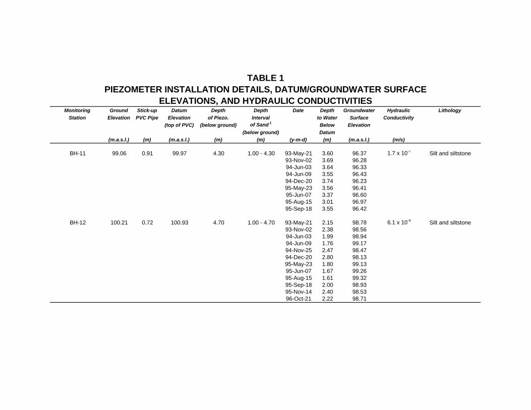
TABLE 1PIEZOMETER INSTALLATION DETAILS, DATUM/GROUNDWATER SURFACE
ELEVATIONS, AND HYDRAULIC CONDUCTIVITIESMonitoring Ground Stick-up Datum Depth Depth Date Depth Groundwater Hydraulic Lithology
Station Elevation PVC Pipe Elevation of Piezo. Interval to Water Surface Conductivity(top of PVC) (below ground) of Sand 1 Below Elevation
(below ground) Datum(m.a.s.l.) (m) (m.a.s.l.) (m) (m) (y-m-d) (m) (m.a.s.l.) (m/s)
BH-11 99.06 0.91 99.97 4.30 1.00 - 4.30 93-May-21 3.60 96.37 1.7 x 10⁻⁷ Silt and siltstone93-Nov-02 3.69 96.2894-Jun-03 3.64 96.3394-Jun-09 3.55 96.4394-Dec-20 3.74 96.2395-May-23 3.56 96.4195-Jun-07 3.37 96.6095-Aug-15 3.01 96.9795-Sep-18 3.55 96.42
BH-12 100.21 0.72 100.93 4.70 1.00 - 4.70 93-May-21 2.15 98.78 6.1 x 10⁻⁹ Silt and siltstone93-Nov-02 2.38 98.5694-Jun-03 1.99 98.9494-Jun-09 1.76 99.1794-Nov-25 2.47 98.4794-Dec-20 2.80 98.1395-May-23 1.80 99.1395-Jun-07 1.67 99.2695-Aug-15 1.61 99.3295-Sep-18 2.00 98.9395-Nov-14 2.40 98.5396-Oct-21 2.22 98.71

TABLE 1PIEZOMETER INSTALLATION DETAILS, DATUM/GROUNDWATER SURFACE
ELEVATIONS, AND HYDRAULIC CONDUCTIVITIESMonitoring Ground Stick-up Datum Depth Depth Date Depth Groundwater Hydraulic Lithology
Station Elevation PVC Pipe Elevation of Piezo. Interval to Water Surface Conductivity(top of PVC) (below ground) of Sand 1 Below Elevation
(below ground) Datum(m.a.s.l.) (m) (m.a.s.l.) (m) (m) (y-m-d) (m) (m.a.s.l.) (m/s)
BH-13 100.57 0.56 101.13 5.00 1.00 - 5.00 93-May-21 1.72 99.42 7.0 x 10⁻⁹ Silt and siltstone93-Nov-02 1.99 99.1494-Jun-03 1.65 99.4994-Jun-09 1.33 99.8094-Dec-20 2.42 98.7195-May-23 1.40 99.7395-Jun-07 1.20 99.9395-Aug-15 1.34 99.7995-Sep-18 1.65 99.4895-Nov-14 2.11 99.0395-Nov-25 2.10 99.0396-Feb-05 2.86 98.2796-Mar-20 2.55 98.5896-Mar-28 2.39 98.7496-Apr-21 1.76 99.3796-May-06 1.56 99.5896-May-15 1.30 99.8396-May-21 1.37 99.7696-May-29 1.50 99.6396-Jun-07 1.47 99.6796-Jun-12 1.59 99.5596-Jun-26 1.46 99.6796-Jul-03 1.49 99.6496-Jul-11 1.41 99.7296-Jul-18 1.41 99.7396-Jul-25 1.54 99.5996-Sep-29 1.68 99.4596-Oct-21 1.74 99.40

TABLE 1PIEZOMETER INSTALLATION DETAILS, DATUM/GROUNDWATER SURFACE
ELEVATIONS, AND HYDRAULIC CONDUCTIVITIESMonitoring Ground Stick-up Datum Depth Depth Date Depth Groundwater Hydraulic Lithology
Station Elevation PVC Pipe Elevation of Piezo. Interval to Water Surface Conductivity(top of PVC) (below ground) of Sand 1 Below Elevation
(below ground) Datum(m.a.s.l.) (m) (m.a.s.l.) (m) (m) (y-m-d) (m) (m.a.s.l.) (m/s)
BH-14 101.41 0.79 102.20 5.00 1.00 - 5.00 94-Jun-03 1.67 100.53 1.2 x 10⁻⁸ Silt and siltstone94-Jun-09 1.12 101.0894-Dec-20 2.26 99.9495-May-23 1.30 100.9095-Jun-07 1.10 101.1095-Aug-15 0.91 101.2995-Sep-18 1.07 101.1395-Nov-14 1.71 100.4996-Feb-05 2.36 99.8496-Mar-28 3.51 98.6996-May-06 1.65 100.5696-May-15 1.22 100.9996-May-21 1.19 101.0296-May-29 1.09 101.1196-Jun-07 1.32 100.8996-Jun-12 1.46 100.7496-Jun-26 1.03 101.1796-Jul-03 0.99 101.2296-Jul-11 1.18 101.0396-Jul-18 1.12 101.0996-Jul-25 1.12 101.0896-Sep-29 1.36 100.8496-Oct-21 1.54 100.66

TABLE 1PIEZOMETER INSTALLATION DETAILS, DATUM/GROUNDWATER SURFACE
ELEVATIONS, AND HYDRAULIC CONDUCTIVITIESMonitoring Ground Stick-up Datum Depth Depth Date Depth Groundwater Hydraulic Lithology
Station Elevation PVC Pipe Elevation of Piezo. Interval to Water Surface Conductivity(top of PVC) (below ground) of Sand 1 Below Elevation
(below ground) Datum(m.a.s.l.) (m) (m.a.s.l.) (m) (m) (y-m-d) (m) (m.a.s.l.) (m/s)
94-15A 99.01 0.65 99.66 3.60 1.80 - 3.60 94-Dec-20 3.58 96.08 2.0 x 10⁻⁸ Sand and gravel/silt till95-May-23 3.46 96.2095-Jun-07 3.16 96.5095-Aug-15 2.78 96.8895-Sep-18 3.32 96.3495-Nov-14 3.65 96.0295-Nov-25 3.66 96.0095-Dec-17 3.66 96.0096-Jan-10 3.70 95.9796-Mar-20 2.25 97.4196-May-06 3.11 96.5596-May-15 2.65 97.0296-May-21 2.67 96.9996-May-29 2.98 96.6996-Jun-07 2.93 96.7496-Jun-12 3.12 96.5596-Jun-26 3.13 96.5396-Jul-03 3.24 96.4396-Jul-11 2.93 96.7496-Jul-18 2.99 96.6796-Jul-25 3.22 96.4596-Sep-29 3.57 96.0996-Oct-21 3.64 96.02

TABLE 1PIEZOMETER INSTALLATION DETAILS, DATUM/GROUNDWATER SURFACE
ELEVATIONS, AND HYDRAULIC CONDUCTIVITIESMonitoring Ground Stick-up Datum Depth Depth Date Depth Groundwater Hydraulic Lithology
Station Elevation PVC Pipe Elevation of Piezo. Interval to Water Surface Conductivity(top of PVC) (below ground) of Sand 1 Below Elevation
(below ground) Datum(m.a.s.l.) (m) (m.a.s.l.) (m) (m) (y-m-d) (m) (m.a.s.l.) (m/s)
94-15C 99.15 0.57 99.72 11.60 9.67 - 11.90 94-Dec-20 2.93 96.79 4.7 x 10⁻⁸ Sandstone and shale95-May-23 2.92 96.8095-Jun-07 2.73 97.0095-Aug-15 2.28 97.4595-Sep-18 2.28 97.4595-Nov-14 2.57 97.1595-Nov-25 2.59 97.1396-Feb-05 2.97 96.7596-Mar-20 2.90 96.8296-Apr-21 2.58 97.1496-May-06 2.53 97.2096-May-15 2.37 97.3696-May-21 2.24 97.4896-May-29 2.31 97.4296-Jun-07 2.26 97.4696-Jun-12 2.35 97.3796-Jun-26 2.39 97.3496-Jul-03 2.40 97.3296-Jul-11 2.30 97.4396-Jul-18 2.27 97.4696-Jul-25 2.35 97.3896-Oct-21 2.58 97.14

TABLE 1PIEZOMETER INSTALLATION DETAILS, DATUM/GROUNDWATER SURFACE
ELEVATIONS, AND HYDRAULIC CONDUCTIVITIESMonitoring Ground Stick-up Datum Depth Depth Date Depth Groundwater Hydraulic Lithology
Station Elevation PVC Pipe Elevation of Piezo. Interval to Water Surface Conductivity(top of PVC) (below ground) of Sand 1 Below Elevation
(below ground) Datum(m.a.s.l.) (m) (m.a.s.l.) (m) (m) (y-m-d) (m) (m.a.s.l.) (m/s)
94-16A 99.18 0.54 99.72 2.82 1.07 - 2.82 94-Dec-20 3.36 96.36 4.5 x 10⁻⁷ Sand/gravel/silt95-May-23 3.21 96.5195-Jun-07 3.01 96.7195-Aug-15 2.71 97.0195-Sep-18 3.23 96.5096-Mar-28 3.80 95.9296-Apr-21 2.78 96.9496-May-06 3.10 96.6296-May-15 2.56 97.1696-May-21 2.58 97.1596-May-29 2.84 96.8896-Jun-07 2.76 96.9796-Jun-12 2.96 96.7696-Jun-26 2.91 96.8296-Jul-03 2.98 96.7596-Jul-11 2.72 97.0196-Jul-18 2.78 96.9596-Jul-25 3.00 96.7396-Sep-29 3.24 96.4896-Oct-21 3.29 96.43

TABLE 1PIEZOMETER INSTALLATION DETAILS, DATUM/GROUNDWATER SURFACE
ELEVATIONS, AND HYDRAULIC CONDUCTIVITIESMonitoring Ground Stick-up Datum Depth Depth Date Depth Groundwater Hydraulic Lithology
Station Elevation PVC Pipe Elevation of Piezo. Interval to Water Surface Conductivity(top of PVC) (below ground) of Sand 1 Below Elevation
(below ground) Datum(m.a.s.l.) (m) (m.a.s.l.) (m) (m) (y-m-d) (m) (m.a.s.l.) (m/s)
94-16B 99.18 0.57 99.75 3.43 2.87 - 3.61 94-Dec-20 3.42 96.33 5.7 x 10⁻⁶ Clayey silt till95-Jan-24 3.43 96.3295-Mar-14 3.45 96.3095-May-23 3.24 96.5195-Jun-07 3.03 96.7295-Aug-15 2.73 97.0295-Sep-18 3.26 96.4995-Nov-14 3.49 96.2795-Nov-25 3.50 96.2595-Dec-17 3.52 96.2396-Jan-10 3.55 96.2096-Feb-05 3.56 96.1996-Feb-06 3.57 96.1896-May-15 2.59 97.1796-May-21 2.61 97.1596-May-29 2.87 96.8996-Jun-07 2.78 96.9796-Jun-12 2.99 96.7696-Jun-26 2.93 96.8396-Jul-03 3.01 96.7596-Jul-11 2.74 97.0196-Jul-18 2.81 96.9596-Jul-25 3.02 96.7396-Sep-29 3.29 96.4696-Oct-21 3.35 96.41

TABLE 1PIEZOMETER INSTALLATION DETAILS, DATUM/GROUNDWATER SURFACE
ELEVATIONS, AND HYDRAULIC CONDUCTIVITIESMonitoring Ground Stick-up Datum Depth Depth Date Depth Groundwater Hydraulic Lithology
Station Elevation PVC Pipe Elevation of Piezo. Interval to Water Surface Conductivity(top of PVC) (below ground) of Sand 1 Below Elevation
(below ground) Datum(m.a.s.l.) (m) (m.a.s.l.) (m) (m) (y-m-d) (m) (m.a.s.l.) (m/s)
94-17A 100.00 0.58 100.59 4.40 1.20 - 4.40 94-Dec-20 3.71 96.88 1.2 x 10⁻⁸ Sandy/silty/gravel tills95-May-23 3.35 97.2495-Jun-07 3.24 97.3595-Aug-15 3.14 97.4595-Sep-18 3.23 97.3695-Nov-14 3.31 97.2895-Nov-25 3.38 97.2195-Dec-17 3.35 97.2496-Jan-10 3.38 97.2196-Feb-05 3.43 97.1696-Feb-06 3.42 97.1796-Mar-20 3.30 97.2996-Mar-28 3.34 97.2596-Apr-21 3.24 97.3596-May-06 3.31 97.2896-May-15 3.09 97.5096-May-21 3.10 97.4996-May-29 3.16 97.4396-Jun-07 3.17 97.4296-Jun-12 3.18 97.4196-Jun-26 3.20 97.3996-Jul-03 3.20 97.3996-Jul-11 3.22 97.3796-Jul-18 3.18 97.4196-Jul-25 3.20 97.3996-Sep-29 3.21 97.3896-Oct-21 3.23 97.36

TABLE 1PIEZOMETER INSTALLATION DETAILS, DATUM/GROUNDWATER SURFACE
ELEVATIONS, AND HYDRAULIC CONDUCTIVITIESMonitoring Ground Stick-up Datum Depth Depth Date Depth Groundwater Hydraulic Lithology
Station Elevation PVC Pipe Elevation of Piezo. Interval to Water Surface Conductivity(top of PVC) (below ground) of Sand 1 Below Elevation
(below ground) Datum(m.a.s.l.) (m) (m.a.s.l.) (m) (m) (y-m-d) (m) (m.a.s.l.) (m/s)
94-18A 99.92 0.54 100.46 3.75 0.60 - 3.75 94-Dec-20 2.25 98.21 5.3 x 10⁻⁸ Cobbles/clayey silt till95-May-23 1.46 99.0095-Jun-07 1.15 99.3195-Aug-15 1.37 99.0995-Sep-18 1.67 98.7995-Nov-14 2.03 98.4395-Nov-25 1.95 98.5196-Feb-05 2.74 97.7296-Mar-17 3.09 97.3796-Mar-20 3.05 97.4196-Apr-21 2.42 98.0496-May-06 1.68 98.7896-May-15 1.47 98.9996-May-21 1.53 98.9396-May-29 1.55 98.9196-Jun-07 1.61 98.8596-Jun-12 1.68 98.7896-Jun-26 1.47 98.9996-Jul-03 1.48 98.9896-Jul-11 1.49 98.9796-Jul-18 1.49 98.9796-Jul-25 1.51 98.9596-Oct-21 1.74 98.72

TABLE 1PIEZOMETER INSTALLATION DETAILS, DATUM/GROUNDWATER SURFACE
ELEVATIONS, AND HYDRAULIC CONDUCTIVITIESMonitoring Ground Stick-up Datum Depth Depth Date Depth Groundwater Hydraulic Lithology
Station Elevation PVC Pipe Elevation of Piezo. Interval to Water Surface Conductivity(top of PVC) (below ground) of Sand 1 Below Elevation
(below ground) Datum(m.a.s.l.) (m) (m.a.s.l.) (m) (m) (y-m-d) (m) (m.a.s.l.) (m/s)
94-19A 98.85 -0.06 98.80 1.70 0.53 - 1.83 94-Dec-20 1.48 97.32 3.3 x 10⁻⁶ Gravel & sand/silty till95-May-23 0.74 98.0695-Jun-07 0.47 98.3295-Aug-15 0.89 97.9195-Sep-18 0.96 97.8495-Nov-14 1.22 97.5896-Apr-21 1.46 97.3496-May-06 1.27 97.5396-May-15 0.80 98.0096-May-21 0.85 97.9596-May-29 0.93 97.8796-Jun-07 0.93 97.8796-Jun-12 0.98 97.8296-Jun-26 0.87 97.9396-Jul-03 0.79 98.0196-Jul-11 0.92 97.8896-Jul-18 0.92 97.8896-Jul-25 0.99 97.8196-Sep-29 1.08 97.7296-Oct-21 1.05 97.75

TABLE 1PIEZOMETER INSTALLATION DETAILS, DATUM/GROUNDWATER SURFACE
ELEVATIONS, AND HYDRAULIC CONDUCTIVITIESMonitoring Ground Stick-up Datum Depth Depth Date Depth Groundwater Hydraulic Lithology
Station Elevation PVC Pipe Elevation of Piezo. Interval to Water Surface Conductivity(top of PVC) (below ground) of Sand 1 Below Elevation
(below ground) Datum(m.a.s.l.) (m) (m.a.s.l.) (m) (m) (y-m-d) (m) (m.a.s.l.) (m/s)
94-19C 99.00 -0.10 98.89 8.64 6.72 - 8.92 94-Dec-20 1.49 97.40 1.1 x 10⁻⁵ Siltstone/sandstone/95-May-23 1.12 97.77 shale95-Jun-07 0.99 97.9195-Aug-15 0.57 98.3295-Sep-18 0.97 97.9395-Nov-14 1.18 97.7196-Apr-21 1.46 97.4396-May-06 1.25 97.6496-May-15 0.86 98.0496-May-21 0.78 98.1296-May-29 0.82 98.0896-Jun-07 0.81 98.0896-Jun-12 0.90 98.0096-Jun-26 0.90 98.0096-Jul-03 0.89 98.0196-Jul-11 0.84 98.0596-Jul-18 0.83 98.0796-Jul-25 0.90 98.0096-Sep-29 1.09 97.8096-Oct-21 1.08 97.81

TABLE 1PIEZOMETER INSTALLATION DETAILS, DATUM/GROUNDWATER SURFACE
ELEVATIONS, AND HYDRAULIC CONDUCTIVITIESMonitoring Ground Stick-up Datum Depth Depth Date Depth Groundwater Hydraulic Lithology
Station Elevation PVC Pipe Elevation of Piezo. Interval to Water Surface Conductivity(top of PVC) (below ground) of Sand 1 Below Elevation
(below ground) Datum(m.a.s.l.) (m) (m.a.s.l.) (m) (m) (y-m-d) (m) (m.a.s.l.) (m/s)
94-20A 98.85 0.54 99.39 2.65 1.37 - 2.70 94-Dec-20 2.26 97.13 2.8 x 10⁻⁷ Clayey silt till95-May-23 2.45 96.9495-Jun-07 1.90 97.4995-Aug-15 1.85 97.5495-Sep-18 2.14 97.2595-Nov-14 2.24 97.1595-Nov-25 2.26 97.1395-Dec-17 2.25 97.1496-Jan-10 2.27 97.1296-Feb-05 2.28 97.1196-Feb-06 2.28 97.1196-Mar-20 1.96 97.4396-Mar-28 2.21 97.1896-Apr-21 1.95 97.4496-May-06 1.99 97.4096-May-15 1.57 97.8296-May-21 1.81 97.5896-May-29 2.02 97.3796-Jun-07 2.02 97.3796-Jun-12 2.12 97.2796-Jun-26 2.02 97.3796-Jul-03 2.05 97.3496-Jul-11 1.96 97.4396-Jul-18 2.03 97.3696-Jul-25 2.14 97.2596-Sep-29 2.17 97.2296-Oct-21 2.19 97.20

TABLE 1PIEZOMETER INSTALLATION DETAILS, DATUM/GROUNDWATER SURFACE
ELEVATIONS, AND HYDRAULIC CONDUCTIVITIESMonitoring Ground Stick-up Datum Depth Depth Date Depth Groundwater Hydraulic Lithology
Station Elevation PVC Pipe Elevation of Piezo. Interval to Water Surface Conductivity(top of PVC) (below ground) of Sand 1 Below Elevation
(below ground) Datum(m.a.s.l.) (m) (m.a.s.l.) (m) (m) (y-m-d) (m) (m.a.s.l.) (m/s)
94-20C 98.97 0.52 99.49 10.05 8.10 - 10.05 94-Dec-20 2.58 96.92 5.2 x 10⁻⁵ Shale and siltstone95-May-23 2.54 96.9695-Jun-07 1.29 98.2195-Aug-15 1.61 97.8895-Sep-18 1.87 97.6395-Nov-14 2.16 97.3395-Nov-25 2.21 97.2895-Dec-17 2.31 97.1896-Jan-10 2.43 97.0696-Feb-05 2.53 96.9696-Feb-06 2.55 96.9496-Mar-20 2.51 96.9896-Mar-28 2.46 97.0396-Apr-21 2.15 97.3496-May-06 2.13 97.3796-May-15 1.90 97.5996-May-21 1.82 97.6896-May-29 1.88 97.6196-Jun-07 1.83 97.6796-Jun-12 1.92 97.5896-Jun-26 1.94 97.5696-Jul-03 1.95 97.5596-Jul-11 1.84 97.6696-Jul-18 1.82 97.6896-Jul-25 1.91 97.5896-Sep-29 2.17 97.3296-Oct-21 2.18 97.32

TABLE 1PIEZOMETER INSTALLATION DETAILS, DATUM/GROUNDWATER SURFACE
ELEVATIONS, AND HYDRAULIC CONDUCTIVITIESMonitoring Ground Stick-up Datum Depth Depth Date Depth Groundwater Hydraulic Lithology
Station Elevation PVC Pipe Elevation of Piezo. Interval to Water Surface Conductivity(top of PVC) (below ground) of Sand 1 Below Elevation
(below ground) Datum(m.a.s.l.) (m) (m.a.s.l.) (m) (m) (y-m-d) (m) (m.a.s.l.) (m/s)
96-21A 98.12 0.60 98.72 4.01 0.91 - 4.27 96-Jun-12 2.10 96.62 Not Tested Sandy silt/cobble till96-Jun-26 2.12 96.6096-Jul-03 2.22 96.5096-Jul-11 1.92 96.8096-Jul-18 1.98 96.7496-Jul-25 2.20 96.5296-Oct-21 2.61 96.11
96-22A 98.52 0.58 99.10 2.13 1.00 - 2.20 96-Jun-26 2.12 96.99 Not Tested Cobble/silt till96-Jul-03 2.27 96.8396-Jul-11 2.05 97.0696-Jul-18 2.11 96.9996-Jul-25 2.29 96.8196-Sep-29 2.29 96.8196-Oct-21 2.50 96.60
96-22B 98.54 0.58 99.11 2.98 2.44 - 3.04 96-Jun-26 2.17 96.94 5.7 x 10⁻⁸ Cobble/silt till96-Jul-03 2.26 96.8596-Jul-11 2.03 97.0996-Jul-18 2.09 97.0296-Jul-25 2.28 96.8396-Sep-29 2.47 96.6496-Oct-21 2.56 96.55

TABLE 1PIEZOMETER INSTALLATION DETAILS, DATUM/GROUNDWATER SURFACE
ELEVATIONS, AND HYDRAULIC CONDUCTIVITIESMonitoring Ground Stick-up Datum Depth Depth Date Depth Groundwater Hydraulic Lithology
Station Elevation PVC Pipe Elevation of Piezo. Interval to Water Surface Conductivity(top of PVC) (below ground) of Sand 1 Below Elevation
(below ground) Datum(m.a.s.l.) (m) (m.a.s.l.) (m) (m) (y-m-d) (m) (m.a.s.l.) (m/s)
96-23A 99.46 0.63 100.09 4.40 1.05 - 4.40 96-Jun-12 3.10 96.99 2.5 x 10⁻⁹ Sandy silt till96-Jun-26 3.08 97.0196-Jul-03 3.22 96.8796-Jul-11 2.95 97.1496-Jul-18 2.95 97.1496-Jul-25 3.11 96.9896-Sep-29 3.22 96.8796-Oct-21 3.29 96.80
96-24A 99.13 0.59 99.72 4.20 1.10 - 4.20 96-Jun-12 2.60 97.12 7.7 x 10⁻⁷ Clayey/silty till96-Jun-26 2.53 97.1996-Jul-03 2.59 97.1396-Jul-11 2.43 97.2996-Jul-18 2.46 97.2696-Jul-25 2.59 97.1396-Sep-29 2.59 97.1396-Oct-21 2.66 97.06
96-25A 99.09 0.57 99.66 2.70 0.80 - 2.70 96-Jun-26 2.84 96.82 Not Tested Silty clay/cobble till96-Jul-03 2.92 96.7496-Jul-11 2.66 97.0096-Jul-18 2.73 96.9396-Jul-25 2.94 96.7296-Sep-29 3.08 96.5896-Oct-21 3.15 96.51

TABLE 1PIEZOMETER INSTALLATION DETAILS, DATUM/GROUNDWATER SURFACE
ELEVATIONS, AND HYDRAULIC CONDUCTIVITIESMonitoring Ground Stick-up Datum Depth Depth Date Depth Groundwater Hydraulic Lithology
Station Elevation PVC Pipe Elevation of Piezo. Interval to Water Surface Conductivity(top of PVC) (below ground) of Sand 1 Below Elevation
(below ground) Datum(m.a.s.l.) (m) (m.a.s.l.) (m) (m) (y-m-d) (m) (m.a.s.l.) (m/s)
96-25B 99.22 0.41 99.63 3.50 2.70 - 3.50 96-Jun-26 2.82 96.82 1.7 x 10⁻⁵ Silt till96-Jul-03 2.89 96.7596-Jul-11 2.63 97.0196-Jul-18 2.68 96.9696-Jul-25 2.91 96.7296-Sep-29 3.07 96.5696-Oct-21 3.14 96.49
96-26A 98.68 0.57 99.26 3.30 0.90 - 3.30 96-Jun-12 2.52 96.74 1.2 x 10⁻⁶ Cobble till96-Jun-26 2.49 96.7796-Jul-03 2.52 96.7496-Jul-11 2.32 96.9496-Jul-18 2.37 96.8996-Jul-25 2.53 96.7396-Sep-29 2.60 96.6696-Oct-21 2.60 96.66

TABLE 1PIEZOMETER INSTALLATION DETAILS, DATUM/GROUNDWATER SURFACE
ELEVATIONS, AND HYDRAULIC CONDUCTIVITIESMonitoring Ground Stick-up Datum Depth Depth Date Depth Groundwater Hydraulic Lithology
Station Elevation PVC Pipe Elevation of Piezo. Interval to Water Surface Conductivity(top of PVC) (below ground) of Sand 1 Below Elevation
(below ground) Datum(m.a.s.l.) (m) (m.a.s.l.) (m) (m) (y-m-d) (m) (m.a.s.l.) (m/s)
CULVERT 1 98.29 0.85 99.14 4.95 0.16 - 4.46 95-Nov-14 3.07 96.07 Not applicable Not applicable95-Nov-25 3.08 96.0696-Feb-05 3.16 95.9896-Mar-17 1.70 97.4496-Mar-28 2.55 96.5996-Apr-17 1.98 97.1696-Apr-21 2.20 96.9496-May-15 1.99 97.1596-May-21 2.01 97.1396-May-29 2.26 96.8896-Jun-07 2.20 96.9496-Jun-12 2.41 96.7396-Jun-26 2.32 96.8296-Jul-03 2.43 96.7196-Jul-11 2.15 96.9996-Jul-18 2.21 96.9396-Jul-25 2.46 96.6896-Aug-01 2.76 96.3896-Aug-02 2.78 96.3696-Aug-05 2.46 96.6896-Aug-07 2.40 96.7496-Aug-10 2.45 96.6996-Aug-12 2.56 96.5896-Aug-14 2.64 96.5096-Aug-15 2.65 96.4996-Aug-16 2.68 96.4696-Sep-29 2.87 96.2796-Oct-21 2.84 96.29

TABLE 1PIEZOMETER INSTALLATION DETAILS, DATUM/GROUNDWATER SURFACE
ELEVATIONS, AND HYDRAULIC CONDUCTIVITIESMonitoring Ground Stick-up Datum Depth Depth Date Depth Groundwater Hydraulic Lithology
Station Elevation PVC Pipe Elevation of Piezo. Interval to Water Surface Conductivity(top of PVC) (below ground) of Sand 1 Below Elevation
(below ground) Datum(m.a.s.l.) (m) (m.a.s.l.) (m) (m) (y-m-d) (m) (m.a.s.l.) (m/s)
CULVERT 2 98.29 0.90 99.18 4.96 N/A 95-Nov-14 3.12 96.06 Not applicable Not applicable96-Mar-28 2.58 96.6096-Apr-17 2.02 97.1696-Apr-21 2.26 96.9296-May-15 2.03 97.1596-May-21 2.06 97.1296-May-29 2.32 96.8796-Jun-07 2.23 96.9696-Jun-12 2.45 96.7496-Jun-26 2.36 96.8296-Jul-03 2.47 96.7196-Jul-11 2.19 97.0096-Jul-18 2.25 96.9396-Jul-25 2.49 96.7096-Aug-01 2.79 96.3996-Aug-02 2.80 96.3896-Aug-05 2.48 96.7096-Aug-07 2.42 96.7696-Aug-10 2.47 96.7296-Aug-11 2.58 96.6196-Aug-12 2.58 96.6196-Aug-14 2.65 96.5396-Aug-15 2.67 96.5196-Aug-16 2.70 96.4896-Sep-29 2.90 96.2896-Oct-21 2.88 96.30

TABLE 1PIEZOMETER INSTALLATION DETAILS, DATUM/GROUNDWATER SURFACE
ELEVATIONS, AND HYDRAULIC CONDUCTIVITIESMonitoring Ground Stick-up Datum Depth Depth Date Depth Groundwater Hydraulic Lithology
Station Elevation PVC Pipe Elevation of Piezo. Interval to Water Surface Conductivity(top of PVC) (below ground) of Sand 1 Below Elevation
(below ground) Datum(m.a.s.l.) (m) (m.a.s.l.) (m) (m) (y-m-d) (m) (m.a.s.l.) (m/s)
CULVERT 3 98.30 0.88 99.17 4.93 N/A 95-Nov-14 3.11 96.07 Not applicable Not applicable96-Mar-28 2.59 96.5896-Apr-17 2.03 97.1496-Apr-21 2.27 96.9196-May-06 2.53 96.6596-May-15 2.02 97.1696-May-21 2.05 97.1396-May-29 2.30 96.8896-Jun-07 2.22 96.9696-Jun-12 2.43 96.7496-Jun-26 2.37 96.8096-Jul-03 2.49 96.6996-Jul-11 2.17 97.0096-Jul-18 2.23 96.9496-Jul-25 2.47 96.7196-Aug-01 2.78 96.3996-Aug-02 2.80 96.3896-Aug-05 2.48 96.6996-Aug-07 2.44 96.7496-Aug-10 2.48 96.6996-Aug-12 2.58 96.6096-Aug-14 2.67 96.5196-Aug-15 2.69 96.4996-Sep-29 2.89 96.2996-Oct-21 2.87 96.31

TABLE 1PIEZOMETER INSTALLATION DETAILS, DATUM/GROUNDWATER SURFACE
ELEVATIONS, AND HYDRAULIC CONDUCTIVITIESMonitoring Ground Stick-up Datum Depth Depth Date Depth Groundwater Hydraulic Lithology
Station Elevation PVC Pipe Elevation of Piezo. Interval to Water Surface Conductivity(top of PVC) (below ground) of Sand 1 Below Elevation
(below ground) Datum(m.a.s.l.) (m) (m.a.s.l.) (m) (m) (y-m-d) (m) (m.a.s.l.) (m/s)
REFERENCE ROD N/A N/A 101.79 N/A N/A 96-Feb-05 1.02 100.77 Not applicable Not applicable96-Mar-28 0.94 100.8596-May-06 0.96 100.8396-May-15 0.92 100.8796-May-21 0.92 100.8796-May-29 0.92 100.8796-Jun-07 0.93 100.8696-Jun-12 0.96 100.8396-Jun-26 0.94 100.8596-Jul-03 0.94 100.8596-Jul-11 0.93 100.8696-Jul-18 0.93 100.8696-Jul-25 0.95 100.8496-Sep-29 1.08 100.71

TABLE 1PIEZOMETER INSTALLATION DETAILS, DATUM/GROUNDWATER SURFACE
ELEVATIONS, AND HYDRAULIC CONDUCTIVITIESMonitoring Ground Stick-up Datum Depth Depth Date Depth Groundwater Hydraulic Lithology
Station Elevation PVC Pipe Elevation of Piezo. Interval to Water Surface Conductivity(top of PVC) (below ground) of Sand 1 Below Elevation
(below ground) Datum(m.a.s.l.) (m) (m.a.s.l.) (m) (m) (y-m-d) (m) (m.a.s.l.) (m/s)
SW CULVERT N/A N/A 101.95 N/A N/A 96-Apr-21 0.96 100.99 Not applicable Not applicable96-May-06 1.05 100.9096-May-15 1.06 100.9096-May-21 1.09 100.8696-May-29 1.25 100.7196-Jun-07 1.38 100.5796-Jun-12 1.64 100.3196-Jun-26 1.25 100.7096-Jul-03 1.15 100.8196-Jul-11 1.35 100.6196-Jul-18 1.26 100.7096-Jul-25 1.59 100.3696-Sep-29 1.72 100.2396-Oct-21 1.86 100.09
Notes:1 For non-standard or previously installed monitoring wells, the screened interval is used instead of the sand interval.N/A = Not applicable.

TABLE 2FIELD MEASURED PARAMETERS
Monitoring Date Temp. Electrical pH Dissolved Eh CommentsStation Conductivity Oxygen
(y-m-d) (°C) (µS/cm) (units) (mg/L) (mV)
BH-1 92-Jun-03 --- 1090 7.50 --- --- Laboratory electrical conductivity93-May-21 8.5 1131 7.27 --- ---93-Nov-02 6.0 1036 6.90 --- ---94-Jun-10 9.0 1060 6.60 --- ---95-Jun-07 10.0 1196 7.03 --- ---95-Nov-14 6.0 985 7.00 --- ---96-Jul-29 12.0 1138 6.93 --- ---96-Oct-21 6.5 996 7.02 --- ---
CW-1 96-Jul-29 13.2 892 6.83 --- ---96-Aug-01 10.1 --- --- 33.5 --- Oxygen sparging experiment in progress96-Aug-02 10.0 --- --- 50.1 --- Oxygen sparging experiment in progress96-Aug-05 11.0 --- --- 8.7 --- Oxygen sparging experiment in progress96-Aug-07 12.1 --- --- 29 --- Oxygen sparging experiment in progress96-Aug-10 11.3 --- --- 41.5 --- Oxygen sparging experiment in progress96-Aug-11 --- --- 6.71 --- --- Oxygen sparging experiment in progress96-Aug-12 11.7 --- --- 19.1 --- Oxygen sparging experiment in progress96-Aug-13 15.0 --- 6.74 37.2 --- Oxygen sparging experiment in progress96-Aug-14 11.4 --- --- 31.8 --- Oxygen sparging experiment in progress96-Aug-15 13.0 --- 6.71 27.6 --- Oxygen sparging experiment in progress96-Aug-16 13.5 --- 6.71 21.8 --- Oxygen sparging experiment in progress96-Oct-21 8.6 896 7.29 --- ---
GW-1 96-May-16 --- --- --- 9.6 19496-May-21 --- --- --- 8.4 12696-May-31 --- --- --- 7.3 12796-Jun-06 5.1 --- --- 3.3 12496-Jun-13 6.2 --- --- 2.8 11596-Jun-26 7.2 --- --- 2.6 30796-Jul-04 --- --- --- 0.7 17796-Jul-11 --- --- --- 1.9 12996-Jul-19 --- --- --- 0.5 15096-Jul-25 --- --- --- --- 32496-Jul-29 11.9 865 7.11 --- ---96-Aug-11 13.5 --- 6.89 --- ---96-Oct-21 9.1 813 7.21 --- ---
MW-1 96-May-16 --- --- --- 0.2 -4896-May-21 --- --- --- 0.1 -2296-May-31 --- --- --- 0.1 -11496-Jun-06 3.1 --- --- 0.3 -9796-Jun-13 3.4 --- --- 4.5 -7096-Jun-26 5.4 --- --- 0.1 -11596-Jul-04 --- --- --- 0.9 -6696-Jul-11 --- --- --- 0.1 -1696-Jul-19 --- --- --- 0.9 -18496-Jul-25 --- --- --- --- -16896-Jul-29 10.0 4110 6.70 --- ---96-Oct-21 9.4 4130 6.73 0.7 -108

TABLE 2FIELD MEASURED PARAMETERS
Monitoring Date Temp. Electrical pH Dissolved Eh CommentsStation Conductivity Oxygen
(y-m-d) (°C) (µS/cm) (units) (mg/L) (mV)
PW-1 95-Jun-07 6.0 1880 6.96 --- ---96-May-16 --- --- --- 0.1 4596-May-21 --- --- --- 1.6 -7796-May-31 --- --- --- 0.2 -12696-Jun-06 2.8 --- --- 2 -9996-Jun-13 4.0 --- --- 5.5 -3996-Jun-26 5.6 --- --- 0.1 -10296-Jul-04 --- --- --- 0.1 -5396-Jul-11 --- --- --- 0.1 -12396-Jul-19 --- --- --- 0.7 -15496-Jul-25 --- --- --- --- -10096-Jul-29 10.0 4680 6.78 --- ---96-Oct-21 9.3 3730 6.91 --- ---
TW-1 96-May-16 --- --- --- 1.8 18396-May-21 --- --- --- 0.2 2796-May-31 --- --- --- 1.2 2196-Jun-06 6.3 --- --- 0.3 -1896-Jun-13 7.6 --- --- 2.6 6696-Jun-26 9.1 --- --- 0.4 2096-Jul-04 --- --- --- 0.7 5996-Jul-11 --- --- --- 0.4 -7896-Jul-19 --- --- --- 0.8 -3196-Jul-25 --- --- --- --- -496-Jul-29 12.0 973 6.72 --- ---96-Oct-21 9.5 960 6.94 --- ---
BH-2 92-Jun-03 --- 691 7.03 --- --- Laboratory electrical conductivity93-May-21 13.5 949 6.74 --- ---93-Nov-02 10.0 662 6.71 --- ---94-Jun-10 12.0 383 7.19 --- ---95-Jun-07 12.0 374 7.22 --- ---95-Nov-14 10.0 587 7.10 --- ---96-May-16 --- --- --- 0.1 -15296-May-21 --- --- --- 0.1 -20996-May-31 --- --- --- 0.1 -24396-Jun-06 8.5 --- --- 0.1 -20896-Jun-13 8.9 --- --- 2.2 1296-Jun-26 11.6 --- --- 0.1 -196-Jul-04 --- --- --- 0.1 4896-Jul-11 --- --- --- 0.1 -18596-Jul-19 --- --- --- 0.1 -4996-Jul-25 --- --- --- --- -18896-Jul-29 13.0 772 6.92 --- ---96-Oct-21 10.1 723 7.01 --- ---

TABLE 2FIELD MEASURED PARAMETERS
Monitoring Date Temp. Electrical pH Dissolved Eh CommentsStation Conductivity Oxygen
(y-m-d) (°C) (µS/cm) (units) (mg/L) (mV)
CW-2 96-Jul-29 11.6 943 7.08 --- ---96-Aug-01 10.1 --- --- 36.3 --- Oxygen sparging experiment in progress96-Aug-02 10.0 --- --- 48.8 --- Oxygen sparging experiment in progress96-Aug-05 11.3 --- --- 9 --- Oxygen sparging experiment in progress96-Aug-07 11.7 --- --- 29 --- Oxygen sparging experiment in progress96-Aug-10 11.4 --- --- 43.6 --- Oxygen sparging experiment in progress96-Aug-11 15.0 --- 6.72 --- --- Oxygen sparging experiment in progress96-Aug-12 11.1 --- --- 24.1 --- Oxygen sparging experiment in progress96-Aug-13 15.0 --- 6.77 37 --- Oxygen sparging experiment in progress96-Aug-14 11.2 --- --- 32.4 --- Oxygen sparging experiment in progress96-Aug-15 13.0 --- 6.79 27.8 --- Oxygen sparging experiment in progress96-Aug-16 13.5 --- 6.81 22.8 --- Oxygen sparging experiment in progress96-Oct-21 8.6 885 6.98 --- ---
GW-2 96-May-16 --- --- --- 5.7 19396-May-21 --- --- --- 5.6 12896-May-31 --- --- --- 3.3 13096-Jun-06 4.5 --- --- 1.3 14496-Jun-13 5.0 --- --- 2 12696-Jun-26 6.3 --- --- 0.1 28496-Jul-04 --- --- --- 0.1 13796-Jul-11 --- --- --- 0.1 12496-Jul-19 --- --- --- 0.1 12696-Jul-25 --- --- --- --- 21296-Jul-29 10.9 904 7.19 --- ---96-Aug-11 14.5 --- 7.02 --- ---96-Oct-21 9.4 908 7.28 --- ---
TW-2 96-May-16 --- --- --- 1.9 17496-May-21 --- --- --- 0.2 5496-May-31 --- --- --- 0.3 3596-Jun-06 6.6 --- --- 0.4 -1096-Jun-13 7.8 --- --- 2.1 8796-Jun-26 9.2 --- --- 0.4 11396-Jul-04 --- --- --- 3 12896-Jul-11 --- --- --- 0.4 -11596-Jul-19 --- --- --- 0.6 -9596-Jul-25 --- --- --- --- -996-Jul-29 13.0 868 6.81 --- ---96-Oct-21 8.9 830 6.92 --- ---
BH-3 92-Jun-03 --- 696 7.40 --- --- Laboratory electrical conductivity93-May-21 5.5 873 6.93 --- --- Hydrocarbon sheen93-Nov-02 7.0 1018 6.78 --- ---94-Jun-10 13.0 391 7.02 --- ---95-Jun-07 12.0 408 7.09 --- ---95-Nov-14 4.5 760 7.28 --- --- Water may have gone into piezometer
upon opening96-Jul-29 12.0 946 6.75 --- ---96-Oct-21 7.7 897 7.00 --- ---

TABLE 2FIELD MEASURED PARAMETERS
Monitoring Date Temp. Electrical pH Dissolved Eh CommentsStation Conductivity Oxygen
(y-m-d) (°C) (µS/cm) (units) (mg/L) (mV)
CW-3 96-Jul-29 12.2 926 7.10 --- ---96-Aug-01 10.2 --- --- 35.9 --- Oxygen sparging experiment in progress96-Aug-02 10.0 --- --- 51.7 --- Oxygen sparging experiment in progress96-Aug-05 11.1 --- --- 7 --- Oxygen sparging experiment in progress96-Aug-07 11.7 --- --- 29.5 --- Oxygen sparging experiment in progress96-Aug-10 11.3 --- --- 43.9 --- Oxygen sparging experiment in progress96-Aug-11 14.5 --- 6.69 --- --- Oxygen sparging experiment in progress96-Aug-12 11.1 --- --- 18.7 --- Oxygen sparging experiment in progress96-Aug-13 14.0 --- 6.76 36.6 --- Oxygen sparging experiment in progress96-Aug-14 11.1 --- --- 34.5 --- Oxygen sparging experiment in progress96-Aug-15 13.0 --- 6.78 27 --- Oxygen sparging experiment in progress96-Aug-16 14.0 --- 6.87 20.7 --- Oxygen sparging experiment in progress96-Oct-21 8.6 930 7.56 --- ---
GW-3 96-May-16 --- --- --- 7.2 19896-May-21 --- --- --- 4.2 13496-May-31 --- --- --- 0.8 11796-Jun-06 5.1 --- --- 1 -10296-Jun-13 5.9 --- --- 1.7 10896-Jun-26 7.2 --- --- 0.1 25896-Jul-04 --- --- --- 0.1 17396-Jul-11 --- --- --- 0.1 15496-Jul-19 --- --- --- 0.1 12296-Jul-25 --- --- --- --- 22896-Jul-29 13.1 971 6.98 --- ---96-Aug-11 12.5 --- 6.84 --- ---96-Oct-21 8.2 914 7.44 --- ---
TW-3 96-May-16 --- --- --- 5.8 17996-May-21 --- --- --- 2 6396-May-31 --- --- --- 4.3 3996-Jun-06 7.1 --- --- 1 3796-Jun-13 8.1 --- --- 3.1 7496-Jun-26 9.9 --- --- 1.6 9796-Jul-04 --- --- --- 3.8 14396-Jul-11 --- --- --- 0.7 1896-Jul-19 --- --- --- 0.9 6196-Jul-25 --- --- --- --- -1096-Jul-29 12.0 845 6.98 --- ---96-Oct-21 9.0 797 7.13 --- ---
BH-4 92-Jun-03 --- 1260 6.72 --- --- Laboratory electrical conductivity93-May-21 16.0 1003 6.89 --- --- Hydrocarbon sheen93-Nov-02 6.5 884 6.78 --- ---94-Jun-10 15.0 552 6.78 --- ---95-Jun-07 14.0 311 6.92 --- ---95-Nov-14 6.0 962 6.90 --- --- Hydrocarbon film on surface96-Jul-29 13.0 743 6.78 --- ---96-Oct-21 7.7 904 7.00 --- --- Strong hydrocarbon odour,
trace free hydrocarbon

TABLE 2FIELD MEASURED PARAMETERS
Monitoring Date Temp. Electrical pH Dissolved Eh CommentsStation Conductivity Oxygen
(y-m-d) (°C) (µS/cm) (units) (mg/L) (mV)
CW-4 96-Jul-29 11.8 948 6.89 --- ---96-Aug-01 10.2 --- --- 36.1 --- Oxygen sparging experiment in progress96-Aug-02 10.0 --- --- 51.4 --- Oxygen sparging experiment in progress96-Aug-05 11.8 --- --- 7.6 --- Oxygen sparging experiment in progress96-Aug-07 11.6 --- --- 30.1 --- Oxygen sparging experiment in progress96-Aug-10 11.3 --- --- 44.2 --- Oxygen sparging experiment in progress96-Aug-11 14.0 --- 6.72 --- --- Oxygen sparging experiment in progress96-Aug-12 11.1 --- --- 19.8 --- Oxygen sparging experiment in progress96-Aug-13 14.5 --- 6.69 36.1 --- Oxygen sparging experiment in progress96-Aug-14 11.2 --- --- 35.6 --- Oxygen sparging experiment in progress96-Aug-15 13.0 --- 6.76 26.7 --- Oxygen sparging experiment in progress96-Aug-16 14.5 --- 6.89 20.6 --- Oxygen sparging experiment in progress
GW-4 96-May-16 --- --- --- 7.2 19796-May-21 --- --- --- 1.1 12796-May-31 --- --- --- 0.4 10996-Jun-06 5.0 --- --- 1 11196-Jun-13 5.9 --- --- 1.7 9996-Jun-26 6.9 --- --- 0.1 25696-Jul-04 --- --- --- 0.1 17496-Jul-11 --- --- --- 0.3 15396-Jul-19 --- --- --- 0.1 11796-Jul-25 --- --- --- --- 29496-Jul-29 11.9 923 6.94 --- ---96-Aug-11 12.0 --- 6.92 --- ---96-Oct-21 8.8 881 7.36 --- ---
TW-4 96-May-16 --- --- --- 3.5 17096-May-21 --- --- --- 2 6096-May-31 --- --- --- 3 13596-Jun-06 7.2 --- --- 0.5 -1996-Jun-13 8.7 --- --- 2.7 6596-Jun-26 9.6 --- --- 1 4996-Jul-04 --- --- --- 2.9 13896-Jul-11 --- --- --- 0.3 -6996-Jul-19 --- --- --- 0.2 -5096-Jul-25 --- --- --- --- -8296-Jul-29 13.0 814 7.00 --- ---96-Oct-21 9.3 795 7.33 --- ---
BH-5 92-Jun-03 --- 1250 6.96 --- --- Laboratory electrical conductivity93-May-21 11.0 1275 6.92 --- --- Hydrocarbon sheen93-Nov-02 7.0 1346 6.88 --- --- Free hydrocarbon94-Jun-10 14.0 1174 6.65 --- ---95-Jun-07 14.0 1205 6.81 --- ---95-Nov-14 5.5 963 6.95 --- --- Hydrocarbon film on surface96-Jul-29 15.0 1178 6.80 --- ---96-Oct-21 7.7 1050 7.10 --- --- Strong hydrocarbon odour,
trace free hydrocarbon

TABLE 2FIELD MEASURED PARAMETERS
Monitoring Date Temp. Electrical pH Dissolved Eh CommentsStation Conductivity Oxygen
(y-m-d) (°C) (µS/cm) (units) (mg/L) (mV)
CW-5 96-Jul-29 12.2 949 7.38 --- ---96-Aug-01 10.5 --- --- 11.4 --- Oxygen sparging experiment in progress96-Aug-11 13.0 --- 7.12 --- --- Oxygen sparging experiment in progress96-Aug-13 14.0 --- 7.76 --- --- Oxygen sparging experiment in progress96-Aug-15 13.5 --- 7.50 --- --- Oxygen sparging experiment in progress96-Aug-16 14.5 --- 7.29 --- --- Oxygen sparging experiment in progress96-Oct-21 8.6 914 7.59 --- ---
TW-5 96-May-16 --- --- --- 0.2 14496-May-21 --- --- --- 0.4 8396-May-31 --- --- --- 0.2 9996-Jun-06 5.8 --- --- 0.2 11596-Jun-13 6.1 --- --- 2.5 7696-Jun-26 7.9 --- --- 0.1 896-Jul-04 --- --- --- 0.1 13896-Jul-11 --- --- --- 0.2 -296-Jul-19 --- --- --- 0.5 2096-Jul-25 --- --- --- --- -396-Jul-29 14.0 883 6.96 --- ---96-Oct-21 9.8 820 6.93 --- ---
BH-6 92-Jun-03 --- 1110 6.89 --- --- Laboratory electrical conductivity93-May-21 7.0 1083 6.80 --- ---93-Nov-02 8.0 1049 6.72 --- --- Hydrocarbon odour94-Jun-10 10.0 909 6.86 --- ---95-Jun-07 8.5 840 6.98 --- ---95-Nov-14 7.0 912 6.90 --- --- Hydrocarbon odour96-May-16 --- --- --- 0.1 -16096-May-21 --- --- --- 0.1 -22896-May-31 --- --- --- 0.1 -29196-Jun-06 4.2 --- --- 0.1 -17096-Jun-13 3.9 --- --- 2.4 -16296-Jun-26 6.4 --- --- 0.1 -13096-Jul-04 --- --- --- 0.3 -18196-Jul-11 --- --- --- 0.1 -23696-Jul-19 --- --- --- 0.1 -16596-Jul-25 --- --- --- --- -22796-Jul-29 13.0 997 6.63 --- ---96-Oct-21 9.1 911 7.00 --- --- Moderate hydrocarbon odour
CW-6 96-Jul-29 14.0 944 7.45 --- ---96-Aug-01 10.6 --- --- 11.3 --- Oxygen sparging experiment in progress96-Aug-11 13.5 --- 7.43 --- --- Oxygen sparging experiment in progress96-Aug-13 14.5 --- 7.67 --- --- Oxygen sparging experiment in progress96-Aug-15 13.5 --- 7.34 --- --- Oxygen sparging experiment in progress96-Aug-16 14.5 --- 7.31 --- --- Oxygen sparging experiment in progress

TABLE 2FIELD MEASURED PARAMETERS
Monitoring Date Temp. Electrical pH Dissolved Eh CommentsStation Conductivity Oxygen
(y-m-d) (°C) (µS/cm) (units) (mg/L) (mV)
TW-6 96-May-16 --- --- --- 0.4 17796-May-21 --- --- --- 2.2 8596-May-31 --- --- --- 0.2 9696-Jun-06 5.8 --- --- 0.2 10596-Jun-13 6.3 --- --- 4.5 5296-Jun-26 8.3 --- --- 0.1 3996-Jul-04 --- --- --- 0.1 13096-Jul-11 --- --- --- 0.3 1196-Jul-19 --- --- --- 0.6 1596-Jul-25 --- --- --- --- 3696-Jul-29 12.0 967 6.85 --- ---96-Oct-21 9.6 839 7.01 --- ---
BH-7 92-Jun-03 --- 1090 6.91 --- --- Laboratory electrical conductivity93-May-21 6.0 1245 6.73 --- ---93-Nov-02 8.0 1222 6.58 --- --- Hydrocarbon odour94-Jun-10 9.0 1130 6.76 --- ---95-Jun-07 5.0 1138 6.92 --- ---95-Nov-14 7.0 1156 6.79 --- --- Hydrocarbon odour96-May-16 --- --- --- 0.1 -14596-May-21 --- --- --- 0.1 -19796-May-31 --- --- --- 0.1 -27196-Jun-06 4.1 --- --- 0.1 -18796-Jun-13 4.0 --- --- 2.6 -7796-Jun-26 5.2 --- --- 0.1 -9396-Jul-04 --- --- --- 0.4 -18296-Jul-11 --- --- --- 0.1 -26096-Jul-19 --- --- --- 0.1 -15996-Jul-25 --- --- --- --- -21196-Jul-29 13.0 1235 6.62 --- ---96-Oct-21 8.0 1191 6.77 --- --- Strong hydrocarbon odour,
trace free product
CW-7 96-Jul-29 13.5 --- 7.39 --- ---96-Aug-01 10.4 --- --- 11.3 --- Oxygen sparging experiment in progress96-Aug-11 13.0 --- 7.48 --- --- Oxygen sparging experiment in progress96-Aug-13 15.0 --- 7.82 --- --- Oxygen sparging experiment in progress96-Aug-15 14.0 --- 7.82 --- --- Oxygen sparging experiment in progress96-Aug-16 14.5 --- 7.75 --- --- Oxygen sparging experiment in progress96-Oct-21 8.6 921 7.57 --- ---
TW-7 96-May-16 --- --- --- 1.7 18696-May-21 --- --- --- 0.3 8996-May-31 --- --- --- 0.8 9896-Jun-06 4.7 --- --- 0.3 6096-Jun-13 5.1 --- --- 10.1 8096-Jun-26 6.6 --- --- 0.1 -7496-Jul-04 --- --- --- 0.2 4096-Jul-11 --- --- --- 0.6 2796-Jul-19 --- --- --- 1.8 2796-Jul-25 --- --- --- --- 5296-Jul-29 11.0 1143 6.86 --- ---96-Oct-21 9.2 1022 6.85 --- ---

TABLE 2FIELD MEASURED PARAMETERS
Monitoring Date Temp. Electrical pH Dissolved Eh CommentsStation Conductivity Oxygen
(y-m-d) (°C) (µS/cm) (units) (mg/L) (mV)
BH-8 92-Jun-03 --- 867 7.45 --- --- Laboratory electrical conductivity93-May-21 7.0 788 7.25 --- ---93-Nov-02 7.0 800 6.99 --- ---94-Jun-10 10.0 769 7.01 --- ---95-Jun-07 9.0 510 7.30 --- ---95-Nov-14 6.5 766 7.24 --- ---96-May-16 --- --- --- 0.1 2896-May-21 --- --- --- 0.1 2996-May-31 --- --- --- 0.4 15396-Jun-06 4.9 --- --- 0.1 -6896-Jun-13 4.8 --- --- 2.4 -4796-Jun-26 5.3 --- --- 0.1 9896-Jul-04 --- --- --- 0.6 2896-Jul-11 --- --- --- 0.1 3196-Jul-19 --- --- --- 0.1 8196-Jul-25 --- --- --- --- -16296-Jul-29 13.0 849 7.11 --- ---96-Oct-21 8.5 766 7.28 --- ---
BH-9 92-Jun-03 --- 1230 7.16 --- --- Laboratory electrical conductivity93-May-21 8.0 1190 7.08 --- ---93-Nov-02 7.0 1151 6.98 --- ---94-Jun-10 8.0 1135 6.93 --- ---95-Jun-07 6.0 933 7.04 --- ---95-Nov-14 --- --- --- --- --- Abandoned
BH-10 92-Jun-03 --- 2260 6.91 --- --- Laboratory electrical conductivity93-May-21 8.0 1595 6.78 --- ---93-Nov-02 7.0 1629 6.63 --- ---94-Jun-10 9.0 1190 6.44 --- ---95-Jun-07 6.0 1225 6.78 --- ---95-Nov-14 8.0 1288 6.81 --- ---96-May-16 --- --- --- 0.1 796-May-21 --- --- --- 0.1 -13596-May-31 --- --- --- 0.1 -9196-Jun-06 2.8 --- --- 0.1 -12096-Jun-13 3.6 --- --- 3.4 -2696-Jun-26 4.9 --- --- 0.1 -8296-Jul-04 --- --- --- 0.9 -6396-Jul-11 --- --- --- 0.2 -10196-Jul-19 --- --- --- 0.5 -12196-Jul-25 --- --- --- --- -8596-Jul-29 8.0 1520 6.90 --- ---96-Oct-21 8.6 1001 6.96 --- ---
BH-11 92-Jun-03 --- 1080 7.64 --- --- Laboratory electrical conductivity93-May-21 8.0 1249 6.92 --- ---93-Nov-02 6.0 1441 6.89 --- ---94-Jun-10 8.0 1208 6.58 --- ---95-Jun-07 5.0 1287 6.81 --- ---95-Nov-14 --- --- --- --- --- Abandoned

TABLE 2FIELD MEASURED PARAMETERS
Monitoring Date Temp. Electrical pH Dissolved Eh CommentsStation Conductivity Oxygen
(y-m-d) (°C) (µS/cm) (units) (mg/L) (mV)
BH-12 92-Jun-03 --- --- --- --- --- 10 mm free hydrocarbon92-Aug-04 --- --- --- --- --- 5 mm free hydrocarbon93-May-21 12.5 1067 6.83 --- --- Free hydrocarbon present93-Nov-02 --- --- --- --- --- 15 mm free hydrocarbon94-Jun-03 --- --- --- --- --- 3 mm free hydrocarbon94-Jun-10 13.0 908 6.43 --- --- Free hydrocarbon present94-Nov-25 --- --- --- --- --- 20 mm free hydrocarbon95-Jun-07 13.0 848 6.84 --- --- 1 mm free hydrocarbon95-Nov-14 8.0 815 6.89 --- --- 8 mm free hydrocarbon96-Jul-29 15.0 863 6.74 --- --- Free hydrocarbon present96-Oct-21 10.2 904 6.91 --- --- Free hydrocarbon present
BH-13 92-Jun-03 --- 1010 7.20 --- --- Laboratory electrical conductivity93-May-21 12.5 916 7.06 --- ---93-Nov-02 10.0 816 6.93 --- --- Hydrocarbon odour94-Jun-10 12.0 877 6.71 --- ---95-Jun-07 15.0 900 6.91 --- ---95-Nov-14 10.5 759 7.16 --- ---96-May-16 --- --- --- 0.1 -18496-Jul-29 16.0 703 6.85 --- --- Slight hydrocarbon sheen96-Oct-21 9.5 712 7.17 --- ---
BH-14 92-Jun-03 --- 1500 6.83 --- --- Laboratory electrical conductivity94-Jun-10 9.0 1443 6.34 --- ---95-Jun-07 6.0 1284 6.85 --- ---95-Nov-14 7.0 1241 6.74 --- ---96-May-16 --- --- --- 1.7 9396-Jul-29 8.0 1346 6.68 --- ---96-Oct-21 7.2 1266 6.79 --- ---
94-15A 94-Dec-20 5.5 1078 7.26 --- ---95-Jun-07 5.0 818 7.05 --- ---95-Nov-14 6.0 905 7.26 --- ---96-May-16 --- --- --- 0.19 17996-May-21 --- --- --- 1.9 9196-May-31 --- --- --- 0.2 9096-Jun-06 6.3 --- --- 0.3 9696-Jun-13 6.6 --- --- 3.1 6596-Jun-26 8.3 --- --- 0.4 -23396-Jul-04 --- --- --- 0.1 13296-Jul-11 --- --- --- 0.3 596-Jul-19 --- --- --- 0.5 2196-Jul-25 --- --- --- --- 1296-Jul-29 11.0 933 6.92 --- ---96-Oct-21 9.6 1031 7.13 --- ---
94-15C 94-Dec-20 6.0 1198 7.09 --- ---95-Jun-07 7.0 1223 7.86 --- ---95-Nov-14 5.5 1150 7.81 --- ---96-May-16 --- --- --- 0.1 16696-Jul-29 9.0 1248 7.64 --- --- Slight hydrocarbon sheen96-Oct-21 6.2 1117 7.87 --- ---

TABLE 2FIELD MEASURED PARAMETERS
Monitoring Date Temp. Electrical pH Dissolved Eh CommentsStation Conductivity Oxygen
(y-m-d) (°C) (µS/cm) (units) (mg/L) (mV)
94-16A 95-Jun-07 6.0 1468 7.02 --- ---96-May-16 --- --- --- 7.8 7496-May-21 --- --- --- 10.2 6196-May-31 --- --- --- 1.9 -796-Jun-06 3.9 --- --- 3.5 -5696-Jun-13 4.7 --- --- 9.3 -1496-Jun-26 7.4 --- --- 2.4 -1096-Jul-04 --- --- --- 1.2 3696-Jul-11 --- --- --- 0.1 -5396-Jul-19 --- --- --- 0.4 -596-Jul-25 --- --- --- --- -7396-Jul-29 12.0 1190 6.98 --- ---96-Oct-21 9.3 1232 7.09 --- ---
94-16B 94-Dec-20 5.5 2010 6.90 --- ---95-Jun-07 5.0 2072 6.99 --- ---95-Nov-14 6.0 1701 6.89 --- ---96-May-16 --- --- --- 1.2 -4296-May-21 --- --- --- 0.6 -5496-May-31 --- --- --- 0.1 -7496-Jun-06 4.5 --- --- 1.1 -6796-Jun-13 5.3 --- --- 6.8 -2596-Jun-26 7.8 --- --- 0.7 -8096-Jul-04 --- --- --- 0.4 -1796-Jul-11 --- --- --- 0.3 -4896-Jul-19 --- --- --- 0.3 -6696-Jul-25 --- --- --- --- -1396-Jul-29 9.0 1664 6.90 --- ---96-Oct-21 9.3 1557 6.96 --- ---
94-17A 94-Dec-20 7.0 1064 7.07 --- --- Hydrocarbon odour95-Jun-07 6.0 1163 7.03 --- ---95-Nov-14 7.5 1024 6.87 --- --- Hydrocarbon sheen and odour96-May-16 --- --- --- 0.1 -10896-May-21 --- --- --- 0.1 -20196-May-31 --- --- --- 0.1 -25896-Jun-06 4.4 --- --- 0.1 -13296-Jun-13 4.7 --- --- 3.7 -12396-Jun-26 5.3 --- --- 0.1 -10096-Jul-04 --- --- --- 0.4 -16296-Jul-11 --- --- --- 0.1 -17796-Jul-19 --- --- --- 0.1 -14896-Jul-25 --- --- --- --- -20396-Jul-29 9.0 1092 6.81 --- --- Slight hydrocarbon sheen96-Oct-21 7.5 963 7.00 --- ---
94-18A 94-Dec-20 4.5 1015 7.16 --- ---95-Jun-07 10.0 1008 6.96 --- ---95-Nov-14 7.0 627 7.17 --- ---96-May-16 --- --- --- 0.1 -8896-Jul-29 15.0 664 6.87 --- ---96-Oct-21 9.2 633 7.16 --- ---

TABLE 2FIELD MEASURED PARAMETERS
Monitoring Date Temp. Electrical pH Dissolved Eh CommentsStation Conductivity Oxygen
(y-m-d) (°C) (µS/cm) (units) (mg/L) (mV)
94-19A 95-Jun-07 9.0 593 7.18 --- ---95-Nov-14 5.0 963 7.40 --- ---96-Jul-29 14.0 838 7.07 --- ---96-Oct-21 6.9 765 7.25 --- ---
94-19C 94-Dec-20 5.0 1071 7.40 --- ---95-Jun-07 5.5 1086 7.43 --- ---95-Nov-14 7.0 1052 7.34 --- ---96-Jul-29 9.0 1032 7.24 --- --- Slight hydrocarbon sheen96-Oct-21 7.4 1066 7.41 --- ---
94-20A 94-Dec-20 5.5 975 7.15 --- ---95-Jun-07 7.0 916 7.10 --- ---95-Nov-14 7.0 920 7.04 --- ---96-May-21 --- --- --- 1.5 8196-May-31 --- --- --- 2.3 8696-Jun-06 8.7 --- --- 1.2 13596-Jun-13 8.4 --- --- 4 28896-Jun-26 9.6 --- --- 0.7 22396-Jul-04 --- --- --- 2 14096-Jul-11 --- --- --- 2.4 18296-Jul-19 --- --- --- 0.3 32896-Jul-25 --- --- --- --- 12896-Jul-29 12.0 970 7.01 --- ---96-Oct-21 7.8 880 7.16 --- ---
94-20C 94-Dec-20 6.0 1145 7.11 --- ---95-Jun-07 6.5 1176 7.27 --- ---95-Nov-14 6.0 1097 7.16 --- ---96-Jul-29 11.0 1174 7.11 --- ---96-Oct-21 7.7 1051 7.24 --- ---
96-21A 96-Jun-13 4.7 --- --- 1.7 9596-Jun-26 5.7 --- --- 0.1 27496-Jul-04 --- --- --- 0.4 2596-Jul-11 --- --- --- 0.1 12996-Jul-19 --- --- --- 0.1 12096-Jul-25 --- --- --- --- 21296-Jul-29 9.0 867 7.19 --- ---96-Aug-11 14.0 --- 6.74 --- ---96-Oct-21 8.6 910 7.34 --- ---
96-22A 96-Jun-13 7.8 --- --- 4.3 7896-Jun-26 8.4 --- --- 2.2 14196-Jul-04 --- --- --- 1.2 2496-Jul-11 --- --- --- 2 -796-Jul-19 --- --- --- 0.5 3896-Jul-25 --- --- --- --- 14896-Jul-29 14.0 910 6.95 --- ---96-Oct-21 9.1 927 7.12 --- ---

TABLE 2FIELD MEASURED PARAMETERS
Monitoring Date Temp. Electrical pH Dissolved Eh CommentsStation Conductivity Oxygen
(y-m-d) (°C) (µS/cm) (units) (mg/L) (mV)
96-22B 96-Jun-13 5.9 --- --- 3.4 8496-Jun-26 7.3 --- --- 0.1 6496-Jul-04 --- --- --- 1 896-Jul-11 --- --- --- 0.1 -4796-Jul-19 --- --- --- 2 1396-Jul-25 --- --- --- --- 10596-Jul-29 12.0 1104 7.10 --- ---96-Oct-21 9.2 1084 7.16 --- ---
96-23A 96-Jun-13 4.0 --- --- 10.2 1496-Jun-26 5.1 --- --- 0.8 3396-Jul-04 --- --- --- 0.9 -2996-Jul-11 --- --- --- 0.5 -5196-Jul-19 --- --- --- 1.5 -2896-Jul-25 --- --- --- --- -3596-Jul-29 8.0 9020 6.28 --- ---96-Oct-21 10.4 9300 5.90 --- ---
96-24A 96-Jun-13 4.4 --- --- 2.6 -3696-Jul-04 --- --- --- 0.9 -5896-Jul-11 --- --- --- 0.1 -10596-Jul-19 --- --- --- 0.8 -5296-Jul-25 --- --- --- --- -3396-Jul-29 10.0 1083 6.85 --- ---96-Oct-21 8.7 870 6.93 --- ---
96-25A 96-Jun-13 4.3 --- --- 7.2 -896-Jun-26 6.1 --- --- 0.4 896-Jul-04 --- --- --- 0.2 -1496-Jul-11 --- --- --- 0.5 -2896-Jul-19 --- --- --- 0.7 396-Jul-25 --- --- --- --- -6196-Jul-29 12.0 946 6.61 --- ---96-Oct-21 8.9 974 6.89 --- ---
96-25B 96-Jun-13 4.1 --- --- 6.4 -4596-Jun-26 6.1 --- --- 0.3 -3396-Jul-04 --- --- --- 0.1 -296-Jul-11 --- --- --- 1.3 -1796-Jul-19 --- --- --- 0.7 -2396-Jul-25 --- --- --- --- -2696-Jul-29 11.0 1111 6.76 --- ---96-Oct-21 9.0 1008 6.78 --- ---
96-26A 96-Jun-13 5.1 --- --- 2.7 3596-Jun-26 7.4 --- --- 0.4 23296-Jul-04 --- --- --- 1.1 -1696-Jul-11 --- --- --- 0.1 6096-Jul-19 --- --- --- 0.1 13796-Jul-25 --- --- --- --- -10996-Jul-29 11.0 1084 6.89 --- ---96-Oct-21 9.0 960 7.06 --- ---

TABLE 2FIELD MEASURED PARAMETERS
Monitoring Date Temp. Electrical pH Dissolved Eh CommentsStation Conductivity Oxygen
(y-m-d) (°C) (µS/cm) (units) (mg/L) (mV)
Culvert 1 96-May-16 --- --- --- 1.6 12196-May-21 --- --- --- 0.1 6996-May-31 --- --- --- 0.1 -3596-Jun-04 --- --- --- 0.1 3396-Jun-06 4.7 --- --- 0.2 -17596-Jun-07 --- --- --- --- -13096-Jun-13 4.9 --- --- 1.8 -9896-Jun-26 6.6 --- --- 7.3 -49596-Jul-04 --- --- --- 0.1 -18196-Jul-11 --- --- --- 0.1 -6796-Jul-19 10.0 --- --- 0.1 -20996-Jul-25 --- --- --- --- -352
Culvert 2 96-May-16 --- --- --- 0.5 7196-May-21 --- --- --- 0.2 56 Hydrocarbon film on surface96-May-31 --- --- --- 3.1 3496-Jun-04 --- --- --- 10.7 16296-Jun-06 5.9 --- --- 9.6 12796-Jun-13 6.3 --- --- 15.5 2296-Jun-26 12.4 --- --- 8 11396-Jul-04 --- --- --- 13.7 10196-Jul-11 --- --- --- 12.7 11696-Jul-19 10.0 --- --- 11.4 10896-Jul-25 --- --- --- --- 10796-Aug-01 --- --- --- 25 --- Oxygen sparging experiment in progress96-Aug-02 --- --- --- 23 --- Oxygen sparging experiment in progress96-Aug-05 10.9 --- --- 12.9 --- Oxygen sparging experiment in progress96-Aug-07 11.4 --- --- 29 --- Oxygen sparging experiment in progress96-Aug-10 11.6 --- --- 32.4 --- Oxygen sparging experiment in progress96-Aug-12 11.1 --- --- 25 --- Oxygen sparging experiment in progress96-Aug-13 11.3 --- --- 34 --- Oxygen sparging experiment in progress96-Aug-14 11.3 --- --- 29.6 --- Oxygen sparging experiment in progress96-Aug-15 11.5 --- --- 25.1 --- Oxygen sparging experiment in progress96-Aug-16 11.3 --- 6.73 18.2 --- Oxygen sparging experiment in progress96-Oct-21 9.3 --- --- --- ---

TABLE 2FIELD MEASURED PARAMETERS
Monitoring Date Temp. Electrical pH Dissolved Eh CommentsStation Conductivity Oxygen
(y-m-d) (°C) (µS/cm) (units) (mg/L) (mV)
Culvert 3 96-May-16 --- --- --- 8 16796-May-21 --- --- --- 9.4 14796-May-31 --- --- --- 3.4 7196-Jun-04 --- --- --- 1.5 15396-Jun-06 4.8 --- --- 2.9 2896-Jun-13 5.4 --- --- 8.6 9096-Jun-26 6.2 --- --- 0.1 2996-Jul-04 --- --- --- 8.4 19596-Jul-11 --- --- --- 5.1 12196-Jul-19 --- --- --- 2.1 13696-Jul-25 --- --- --- --- 16596-Aug-02 --- --- --- 10.6 --- Oxygen sparging experiment in progress96-Aug-05 10.7 --- --- 12 --- Oxygen sparging experiment in progress96-Aug-07 11.5 --- --- 12 --- Oxygen sparging experiment in progress96-Aug-10 11.4 --- --- 13.6 --- Oxygen sparging experiment in progress96-Aug-12 11.2 --- --- 14.2 --- Oxygen sparging experiment in progress96-Aug-13 12.6 --- --- 13.5 --- Oxygen sparging experiment in progress96-Aug-14 11.9 --- --- 13.3 --- Oxygen sparging experiment in progress96-Aug-15 13.5 --- --- 12.4 --- Oxygen sparging experiment in progress96-Aug-16 12.0 --- --- 12 --- Oxygen sparging experiment in progress
Reference 96-Oct-21 1.0 860 7.06 --- ---Rod
Water Well 94-Jun-10 8.0 1133 8.33 --- ---95-Jun-07 8.0 1259 8.70 --- ---96-Oct-21 7.4 1010 8.82 --- ---
Notes:Electrical Conductivity normalized to 25 °C.

TABLE 3MAJOR ION GROUNDWATER CHARACTERIZATION
AND MINERALIZATION
Monitoring Date Calcium Magnesium Sodium Potassium Bicarbonate Sulphate Chloride Ion TDSStation Balance
(y-m-d) (mg/L) (mg/L) (mg/L) (mg/L) (mg/L) (mg/L) (mg/L) (balance) (mg/L)Water Quality Guidelines (mg/L) 200 500 250 500
BH-1 95-Nov-14 163 38.5 15.1 3.3 680 28.8 6.7 0.98 614*96-Jul-29 171 39.8 14.1 3.19 742 15.3 9.3 0.98 628*96-Oct-22 170 42.0 14.7 3.04 741 15.0 11.0 0.95 657*
CW-1 95-Nov-15 156 39.6 31.0 4.6 661 7.6 30.0 0.97 579*96-Jul-29 127 34.5 23.1 5.96 584 <0.1 7.8 1.05 49296-Oct-22 125 37.7 31.5 5.84 645 3.4 21.1 0.96 549*
GW-1 95-Nov-14 113 35.1 26.2 5.7 590 12.2 10.2 0.96 49896-Jul-29 115 29.4 19.7 8.1 538 0.2 10.3 0.99 46496-Oct-22 135 33.3 22.8 8.54 590 11.4 9.6 1.05 517*
MW-1 95-Nov-15 365 180 97.9 9.7 662 4.0 903* 1.03 1890*96-Jul-29 260 105 64.3 8.69 690 9.2 483* 0.98 1281*96-Oct-22 349 194 104 8.72 701 3.8 998* 0.96 2008*
PW-1 95-Jun-07 330 141 91.0 6.7 745 9.4 666* 1.03 1630*95-Nov-15 418 190 109 8.1 640 5.2 1020* 1.05 2070*96-Jul-29 299 140 74.9 7.76 594 10.9 730* 0.98 1565*96-Oct-22 332 182 99.3 8.55 646 6.0 976* 0.94 1927*
TW-1 95-Nov-15 165 43.7 31.5 4.0 657 6.4 46.9 1.09 626*96-Jul-30 139 36.8 23.0 5.31 645 <0.1 <0.5 1.05 527*96-Oct-22 142 40.5 30.1 4.14 639 2.5 31.8 1.04 570*

TABLE 3MAJOR ION GROUNDWATER CHARACTERIZATION
AND MINERALIZATION
Monitoring Date Calcium Magnesium Sodium Potassium Bicarbonate Sulphate Chloride Ion TDSStation Balance
(y-m-d) (mg/L) (mg/L) (mg/L) (mg/L) (mg/L) (mg/L) (mg/L) (balance) (mg/L)Water Quality Guidelines (mg/L) 200 500 250 500
BH-2 95-Nov-15 97.5 13.3 16.2 11.5 408 9.8 1.7 1.00 35496-Jul-29 128 12.4 9.15 10.5 491 <0.1 <0.5 1.00 40696-Oct-22 145 16.2 9.43 10.6 530 3.7 0.8 1.05 451
CW-2 95-Nov-15 157 37.1 37.1 4.4 668 10.1 36.7 0.99 606*96-Jul-29 133 35.1 22.3 5.75 624 <0.1 7.4 1.02 516*96-Oct-22 119 33.6 32.0 7.01 595 5.1 23.8 0.97 519*
GW-2 95-Nov-14 124 33.9 32.6 4.2 622 18.8 23.4 0.93 548*96-Jul-29 120 31.8 29.7 8.83 562 14.3 15.5 1.02 502*96-Oct-22 140 36.7 51.0 9.09 622 13.8 30.4 1.10 592*
TW-2 96-Jul-30 123 32.3 22.2 6.55 575 <0.1 <0.5 1.05 47296-Oct-22 130 36.5 25.4 3.96 618 2.8 6.2 1.03 518*
BH-3 95-Nov-14 84.3 14.9 69.9 1.5 432 23.8 44.0 0.94 46796-Jul-29 131 27.4 16.3 1.78 618 <0.1 10.6 0.91 49796-Oct-22 157 33.4 13.1 15.0 653 2.4 6.4 1.02 541*
CW-3 95-Nov-15 145 38.6 35.7 4.8 653 8.8 35.6 1.02 596*96-Jul-29 126 33.2 21.5 5.93 597 <0.1 7.8 1.01 49596-Oct-22 141 39.6 33.6 6.71 649 4.1 25.0 1.04 578*
GW-3 95-Nov-14 127 32.4 30.9 4.0 608 8.6 34.1 0.94 543*96-Jul-29 132 37.5 26.6 8.09 636 <0.1 16.5 1.01 539*96-Oct-22 147 40.9 36.9 8.33 713 5.5 23.7 1.00 620*

TABLE 3MAJOR ION GROUNDWATER CHARACTERIZATION
AND MINERALIZATION
Monitoring Date Calcium Magnesium Sodium Potassium Bicarbonate Sulphate Chloride Ion TDSStation Balance
(y-m-d) (mg/L) (mg/L) (mg/L) (mg/L) (mg/L) (mg/L) (mg/L) (balance) (mg/L)Water Quality Guidelines (mg/L) 200 500 250 500
TW-3 96-Jul-30 112 28.6 20.9 6.96 535 0.4 9.3 0.99 45096-Oct-22 122 30.1 25.4 7.36 518 14.0 17.9 1.06 479
BH-4 95-Nov-14 150 32.0 13.0 2.32 690 0.7 8.4 0.93 551*96-Jul-29 118 17.7 9.76 2.57 501 <0.1 <0.5 0.95 39996-Oct-22 151 27.7 12.1 2.17 627 2.3 4.8 0.99 513*
CW-4 95-Nov-15 146 39.7 36.9 4.8 659 9.1 35.2 1.02 602*96-Jul-29 129 35.2 22.7 6.00 614 <0.1 7.6 1.02 508*
GW-4 95-Nov-14 122 30.4 29.2 3.6 569 10.5 22.6 0.97 505*96-Jul-29 135 36.4 28.9 8.91 628 0.2 16.1 1.04 539*96-Oct-22 129 37.2 30.8 7.44 600 5.3 20.6 1.05 532*
TW-4 95-Nov-15 147 29.7 28.8 3.6 558 12.2 28.0 1.09 530*96-Jul-30 109 28.0 20.3 7.35 521 0.4 11.0 0.99 43996-Oct-22 112 22.8 50.7 8.28 433 21.0 58.0 1.07 491
BH-5 93-Nov-02 182 49.0 21.6 1.8 734 <0.1 65.2 1.02 687*94-Jun-10 155 43.0 20.6 2.05 720 1.1 18.3 0.99 600*95-Jun-07 170 44.2 19.5 1.9 763 0.2 18.9 1.00 636*95-Nov-14 134 39.6 17.8 2.0 641 4.3 9.0 0.99 527*96-Jul-29 158 41.1 20.8 2.38 752 1.0 11.7 0.96 611*96-Oct-22 155 42.5 20.1 2.43 683 1.2 12.9 1.05 576*

TABLE 3MAJOR ION GROUNDWATER CHARACTERIZATION
AND MINERALIZATION
Monitoring Date Calcium Magnesium Sodium Potassium Bicarbonate Sulphate Chloride Ion TDSStation Balance
(y-m-d) (mg/L) (mg/L) (mg/L) (mg/L) (mg/L) (mg/L) (mg/L) (balance) (mg/L)Water Quality Guidelines (mg/L) 200 500 250 500
CW-5 95-Nov-15 153 37.7 34.8 4.6 663 9.2 41.1 1.01 613*96-Jul-29 130 35.8 22.8 5.78 638 <0.1 7.3 0.99 521*96-Oct-22 135 38.5 33.3 6.95 629 5.5 25.3 1.03 562*
TW-5 95-Nov-15 158 33.7 34.2 3.9 624 12.9 34.2 1.07 591*96-Jul-30 118 30.6 22.9 7.41 566 0.4 <0.5 1.02 46996-Oct-22 116 31.7 27.0 8.27 539 9.4 12.2 1.04 474
BH-6 93-May-21 130 47.0 15.0 2.04 708 3.3 3.1 0.94 555*93-Nov-02 134 48.5 19.2 2.1 694 <0.1 4.0 1.01 555*94-Jun-10 130 38.9 15.1 1.25 655 2.5 2.4 0.96 517*95-Jun-07 97.6 25.5 8.1 0.9 545 2.0 4.2 --- 41195-Nov-15 132 47.8 17.7 2.1 675 2.1 5.3 1.01 545*96-Jul-29 120 42.5 15.1 1.67 667 <0.1 <0.5 0.93 513*96-Oct-22 135 46.3 16.4 1.65 664 0.7 4.8 1.02 537*
CW-6 95-Nov-15 146 36.8 33.7 4.7 664 9.0 35.2 0.99 598*96-Jul-29 130 34.7 22.1 5.67 628 <0.1 7.1 1.00 514*
TW-6 95-Nov-15 147 31.0 32.3 3.3 631 15.6 25.0 1.00 572*96-Jul-30 118 31.6 22.7 6.92 622 0.4 12.6 0.91 505*96-Oct-22 131 33.9 27.3 8.52 568 15.9 13.7 1.06 519*

TABLE 3MAJOR ION GROUNDWATER CHARACTERIZATION
AND MINERALIZATION
Monitoring Date Calcium Magnesium Sodium Potassium Bicarbonate Sulphate Chloride Ion TDSStation Balance
(y-m-d) (mg/L) (mg/L) (mg/L) (mg/L) (mg/L) (mg/L) (mg/L) (balance) (mg/L)Water Quality Guidelines (mg/L) 200 500 250 500
BH-7 93-May-21 167 57.5 18.8 1.87 855 3.6 6.9 0.98 683*93-Nov-02 189 61.5 24.2 2.1 878 41.9 8.6 1.01 766*94-Jun-10 153 56.0 14.6 1.78 806 1.0 8.3 0.96 638*95-Jun-07 169 57.9 10.0 1.6 568 0.1 8.3 1.43 531*95-Nov-15 166 64.3 11.0 1.7 845 1.1 6.4 1.00 673*96-Jul-29 166 59.9 11.0 1.45 852 0.4 6.4 0.97 671*96-Oct-22 187 62.9 11.9 1.33 934 1.5 6.4 0.97 742*
CW-7 95-Nov-15 144 36.8 34.7 4.7 653 8.9 35.7 0.99 592*96-Jul-29 116 32.0 20.5 5.35 603 <0.1 7.3 0.94 48496-Oct-22 129 39.3 34.3 6.73 658 4.2 24.7 0.97 571*
TW-7 95-Nov-15 158 34.7 85.5 3.7 681 23.1 82.9 1.04 729*96-Jul-30 128 35.4 62.0 7.29 644 4.3 76.5 0.95 636*96-Oct-22 162 50.2 21.5 4.97 739 6.9 1.3 1.08 617*
BH-8 93-May-21 82.5 37.1 34.1 3.37 495 9.0 4.5 1.04 41893-Nov-02 76.5 43.0 38.2 3.9 545 8.9 5.4 0.98 44894-Jun-10 77.0 39.6 35.8 3.92 529 9.7 5.2 0.97 43695-Jun-07 58.4 21.9 10.2 2.8 271 8.2 3.0 1.04 26195-Nov-15 87.6 44.4 37.9 4.2 551 10.6 5.1 1.04 46596-Jul-29 75.2 41.5 36.5 3.64 549 <0.1 <0.5 0.98 43296-Oct-22 81.9 47.0 40.8 4.01 556 8.9 6.0 1.04 467

TABLE 3MAJOR ION GROUNDWATER CHARACTERIZATION
AND MINERALIZATION
Monitoring Date Calcium Magnesium Sodium Potassium Bicarbonate Sulphate Chloride Ion TDSStation Balance
(y-m-d) (mg/L) (mg/L) (mg/L) (mg/L) (mg/L) (mg/L) (mg/L) (balance) (mg/L)Water Quality Guidelines (mg/L) 200 500 250 500
BH-9 93-May-21 99.0 40.5 108 5.08 731 32.2 25.0 0.98 676*93-Nov-02 89.0 41.0 116 5.2 714 31.0 27.7 0.99 667*94-Jun-10 94.5 39.9 123 5.05 709 31.8 27.0 1.03 676*95-Jun-07 97.1 41.4 57.8 4.4 601 18.8 13.6 0.99 556*
BH-10 95-Nov-15 152 53.8 59.4 7.8 723 9.4 81.8 1.03 726*96-Jul-29 148 50.1 60.3 8.73 641 10.8 131 0.99 736*96-Oct-22 127 46.1 52.5 8.04 673 8.2 42.4 1.02 623*
BH-12 95-Nov-15 136 29.0 28.0 4.8 591 1.1 4.5 1.07 49996-Jul-29 116 24.8 23.9 5.64 566 <0.1 <0.5 0.97 45396-Oct-22 153 30.5 22.5 5.84 624 0.4 3.3 1.09 528*
BH-13 95-Nov-15 110 27.1 45.3 3.1 518 15.2 8.8 1.08 46996-Jul-29 91.6 18.8 22.7 3.49 419 0.2 <0.5 1.04 34896-Oct-22 110 24.8 29.1 3.44 483 10.2 7.5 1.06 427
BH-14 95-Nov-14 183 71.2 19.4 3.0 928 12.1 30.4 0.98 783*96-Jul-29 182 74.3 20.7 3.39 870 12.4 28.7 1.05 757*96-Oct-21 212 72.9 20.5 2.92 940 15.2 30.1 1.06 824*
94-15A 95-Nov-15 109 36.5 46.9 5.9 602 18.6 33.5 0.95 553*96-Jul-29 124 33.7 26.0 8.0 585 0.4 14.1 1.02 507*96-Oct-22 128 41.1 72.5 6.6 596 52.5 35.1 1.06 667*

TABLE 3MAJOR ION GROUNDWATER CHARACTERIZATION
AND MINERALIZATION
Monitoring Date Calcium Magnesium Sodium Potassium Bicarbonate Sulphate Chloride Ion TDSStation Balance
(y-m-d) (mg/L) (mg/L) (mg/L) (mg/L) (mg/L) (mg/L) (mg/L) (balance) (mg/L)Water Quality Guidelines (mg/L) 200 500 250 500
94-15C 95-Nov-15 17.7 6.9 295* 2.8 756 84.2 0.5 1.01 786*96-Jul-29 18.0 6.32 271* 2.4 758 79.5 <0.5 0.94 757*96-Oct-22 20.5 7.71 293* 2.67 745 83.7 0.5 1.04 781*
94-16A 96-Jul-29 174 35.9 30.8 10.5 714 15.9 33.1 1.00 675*96-Oct-22 183 42.8 41.2 15.7 880 11.0 29.7 0.94 780*
94-16B 95-Nov-15 216 56.5 65.8 11.0 852 25.2 159 0.98 960*96-Jul-29 196 53.9 69.5 9.54 759 20.0 171 0.99 900*96-Oct-22 195 51.3 63.5 10.2 907 15.4 90.2 0.96 880*
94-17A 95-Nov-15 143 47.8 31.5 4.1 729 1.2 11.4 1.02 604*96-Jul-29 146 49.7 26.4 4.26 762 0.7 9.0 0.99 617*96-Oct-22 145 50.4 29.8 3.88 730 0.7 4.7 1.05 600*
94-18A 95-Nov-15 104 19.8 16.0 1.2 440 16.0 4.7 0.98 38296-Jul-29 94.3 17.7 13.8 1.0 405 <0.1 <0.5 1.02 32996-Oct-22 100 19.7 14.6 0.95 442 10.6 4.6 0.96 372
94-19A 95-Nov-14 104 40.7 61.0 2.07 570 93.1 5.4 0.96 609*96-Jul-29 102 23.7 70.3 2.86 553 16.3 <0.5 1.07 49996-Oct-21 122 34.2 32.1 15.0 531 34.2 2.9 1.07 501*
94-19C 95-Nov-14 30.7 11.9 138 2.56 490 40.9 2.8 0.96 47296-Jul-29 40.6 17.3 188 3.35 698 39.2 1.6 0.95 640*96-Oct-21 47.1 19.1 207* 3.55 705 44.4 2.8 1.04 677*

TABLE 3MAJOR ION GROUNDWATER CHARACTERIZATION
AND MINERALIZATION
Monitoring Date Calcium Magnesium Sodium Potassium Bicarbonate Sulphate Chloride Ion TDSStation Balance
(y-m-d) (mg/L) (mg/L) (mg/L) (mg/L) (mg/L) (mg/L) (mg/L) (balance) (mg/L)Water Quality Guidelines (mg/L) 200 500 250 500
94-20A 95-Nov-14 136 37.3 20.3 4.67 677 10.2 8.1 0.94 556*96-Jul-29 131 34.4 20.5 5.25 620 0.2 7.7 1.00 510*96-Oct-21 156 39.7 20.2 5.17 647 7.7 7.1 1.10 562*
94-20C 95-Nov-14 67.2 36.1 162 4.5 803 27.8 <0.5 0.98 699*96-Jul-29 64.8 39.7 157 5.09 792 23.4 <0.5 1.00 687*96-Oct-21 81.6 37.5 166 4.59 811 25.2 0.5 1.05 721*
96-21A 96-Jul-29 112 32.9 16.7 9.35 539 0.2 22.7 0.98 46496-Oct-22 127 39.2 37.6 7.87 611 6.6 29.9 1.03 555*
96-22A 96-Jul-30 129 32.4 24.2 8.61 572 14.1 15.4 1.01 520*96-Oct-22 146 40.0 25.7 9.32 624 24.8 13.0 1.07 571*
96-22B 96-Jul-30 112 40.4 76.9 6.3 653 46.8 54.0 0.94 663*96-Oct-22 144 42.8 76.8 5.99 680 55.9 25.7 1.09 691*
96-23A 96-Jul-29 1260 543 123 14.1 2436 8.0 1770* 1.25 4936*96-Oct-22 1710 595 137 15.5 2926 8.1 1760* 1.44 5689*
96-24A 96-Jul-29 119 38.7 28.7 3.18 649 <0.1 9.8 0.96 524*96-Oct-22 120 42.5 30.1 3.58 640 1.3 9.8 1.01 527*
96-25A 96-Jul-30 108 35.3 36.1 12.9 608 <0.1 11.7 0.99 508*96-Oct-22 128 41.3 38.0 12.1 678 5.3 21.0 0.99 585*

TABLE 3MAJOR ION GROUNDWATER CHARACTERIZATION
AND MINERALIZATION
Monitoring Date Calcium Magnesium Sodium Potassium Bicarbonate Sulphate Chloride Ion TDSStation Balance
(y-m-d) (mg/L) (mg/L) (mg/L) (mg/L) (mg/L) (mg/L) (mg/L) (balance) (mg/L)Water Quality Guidelines (mg/L) 200 500 250 500
96-25B 96-Jul-30 124 41.0 65.4 11.4 701 6.4 22.1 1.04 621*96-Oct-22 138 43.4 44.0 6.99 695 3.1 30.5 1.02 613*
96-26A 96-Jul-30 145 49.4 29.8 6.95 725 4.4 19.6 1.02 618*96-Oct-22 140 46.5 42.5 7.47 691 8.2 15.2 1.08 606*
Reference Rod 96-Oct-22 145 38.1 31.2 6.26 605 0.8 29.7 1.10 554*
Water Well 94-Jun-10 2 0.3 274* 1.03 678 35.7 5.2 0.94 681*95-Jun-07 1.6 0.7 292* 1.1 680 30.9 4.7 1.01 696*95-Nov-15 2 0.4 293* 0.9 680 39.7 5.2 1.01 702*96-Oct-22 1.95 0.46 284* 0.94 678 38.4 5.2 0.99 687*
Notes:1.* Denotes Values That Exceed Water Quality Guidelines (mg/L).2. Carbonate concentrations are less than the detection limit of 0.5 mg/L for all analyses except the water well, which averages approximately 20 mg/L.

TABLE 4DISSOLVED HYDROCARBONS AND DISSOLVED ORGANIC CARBON
Monitoring Date Benzene Ethylbenzene Toluene Xylenes BTEX DOC TPH TPH Station (total) (total) Vol. (C 6 -C 11 ) Semi-Vol. (C 12 -C 22 )
(mg/L) (mg/L) (mg/L) (mg/L) (mg/L) (mg/L) (mg/L) (mg/L)Water Quality Guidelines (mg/L) 0.005 ≤ 0.0024 ≤ 0.024 ≤ 0.3
BH-1 92-Aug-06 <0.001 <0.001 <0.001 <0.001 <1 <193-May-21 <0.001 <0.001 <0.001 <0.001 <1 <193-Nov-02 <0.001 <0.001 <0.001 <0.001 <1 <194-Jun-10 <0.001 <0.001 <0.001 0.001 0.001 <1 <195-Jun-07 <0.001 <0.001 <0.001 <0.001 <1 <195-Nov-14 <0.001 <0.001 <0.001 <0.001 9.6 <1 <196-Jul-30 <0.001 <0.001 <0.001 <0.001 <1 <196-Oct-21 <0.001 <0.001 <0.001 <0.001 <1 <196-Oct-22 12.5
BH-1 Dup. 96-Oct-21 <0.001 <0.001 <0.001 <0.001 <1 <1
CW-1 95-Nov-15 0.009* <0.001 <0.001 0.001 0.010* 8.2 <1 <196-Apr-21 0.006* <0.001 0.001 <0.001 0.007* <1 <196-May-05 <0.001 <0.001 <0.001 <0.001 <1 <196-May-15 0.013* <0.001 0.003 0.002 0.018* <1 <196-Jun-12 0.009* <0.001 <0.001 0.002 0.011* <1 <196-Jul-03 0.013* 0.001 <0.001 0.003 0.017* <1 <196-Jul-29 0.0073* <0.0004 <0.0004 <0.0008 0.0073*96-Jul-30 0.036* 0.001 <0.001 0.001 0.038* <1 <196-Oct-21 0.011* <0.001 <0.001 <0.001 0.011* <1 <196-Oct-22 11.0
CW-1 Dup. 95-Nov-15 0.008* <0.001 <0.001 0.001 0.009* <1 <196-May-15 0.007* <0.001 0.002 <0.001 0.009* <1 <196-Jul-03 0.012* <0.001 <0.001 0.002 0.014* <1 <196-Oct-21 0.017* <0.001 <0.001 <0.001 0.017* <1 <1

TABLE 4DISSOLVED HYDROCARBONS AND DISSOLVED ORGANIC CARBON
Monitoring Date Benzene Ethylbenzene Toluene Xylenes BTEX DOC TPH TPH Station (total) (total) Vol. (C 6 -C 11 ) Semi-Vol. (C 12 -C 22 )
(mg/L) (mg/L) (mg/L) (mg/L) (mg/L) (mg/L) (mg/L) (mg/L)Water Quality Guidelines (mg/L) 0.005 ≤ 0.0024 ≤ 0.024 ≤ 0.3
DW-1 96-May-15 <0.001 <0.001 <0.001 <0.001 <1 <196-Jun-12 <0.001 <0.001 <0.001 <0.001 <1 <196-Jul-03 <0.001 <0.001 <0.001 <0.001 <1 <196-Jul-30 <0.001 <0.001 <0.001 <0.001 <1 <1
DW-1 Dup. 96-May-15 <0.001 <0.001 <0.001 <0.001 <1 <1
GW-1 95-Nov-14 7.395-Nov-15 <0.001 <0.001 <0.001 <0.001 <1 <196-Apr-21 <0.001 <0.001 <0.001 <0.001 <1 <196-May-05 <0.001 <0.001 <0.001 <0.001 <1 <196-May-15 <0.001 <0.001 <0.001 <0.001 <1 <196-Jun-12 <0.001 <0.001 <0.001 <0.001 <1 <196-Jul-03 <0.001 <0.001 <0.001 <0.001 <1 <196-Jul-30 <0.001 <0.001 <0.001 <0.001 <1 <196-Aug-18 <0.001 <0.001 <0.001 <0.001 <1 <196-Aug-27 <0.001 <0.001 <0.001 <0.001 <1 <196-Oct-22 8.796-Oct-28 <0.001 <0.001 <0.001 <0.001 <1 <1
MW-1 95-Nov-15 <0.001 <0.001 <0.001 <0.001 8.6 <1 <196-May-15 0.004 <0.001 <0.001 <0.001 0.004 <1 <196-Jun-12 0.002 <0.001 <0.001 <0.001 0.002 <1 <196-Jul-03 0.006* <0.001 <0.001 <0.001 0.006* <1 <196-Jul-30 <0.001 <0.001 <0.001 <0.001 <1 <196-Oct-21 <0.001 <0.001 <0.001 <0.001 <1 <196-Oct-22 8.4

TABLE 4DISSOLVED HYDROCARBONS AND DISSOLVED ORGANIC CARBON
Monitoring Date Benzene Ethylbenzene Toluene Xylenes BTEX DOC TPH TPH Station (total) (total) Vol. (C 6 -C 11 ) Semi-Vol. (C 12 -C 22 )
(mg/L) (mg/L) (mg/L) (mg/L) (mg/L) (mg/L) (mg/L) (mg/L)Water Quality Guidelines (mg/L) 0.005 ≤ 0.0024 ≤ 0.024 ≤ 0.3
PW-1 95-Jun-07 <0.001 <0.001 <0.001 <0.001 12.9 <1 <195-Nov-15 <0.001 <0.001 <0.001 <0.001 6.6 <1 <196-May-15 <0.001 <0.001 <0.001 <0.001 <1 <196-Jun-12 <0.001 <0.001 <0.001 <0.001 <1 <196-Jul-03 <0.001 <0.001 <0.001 <0.001 <1 <196-Jul-30 <0.001 <0.001 <0.001 <0.001 <1 <196-Oct-21 <0.001 <0.001 <0.001 <0.001 <1 <196-Oct-22 7.5
PW-1 Dup. 96-Jul-30 <0.001 <0.001 <0.001 <0.001 <1 <1
TW-1 95-Nov-15 0.007* <0.001 <0.001 <0.001 0.007* 8.1 <1 <196-Apr-21 0.066* 0.001 0.016 0.012 0.095* <1 <196-May-15 0.043* 0.001 0.011 0.013 0.068* <1 <196-Jun-12 0.064* 0.005* <0.001 0.021 0.090* <1 <196-Jul-03 0.065* 0.004* <0.001 0.015 0.084* <1 <196-Jul-30 0.045* 0.002 <0.001 0.004 0.051* <1 <196-Aug-18 0.046* 0.002 <0.001 0.005 0.053* <1 <196-Aug-27 0.037* 0.002 <0.001 0.003 0.042* <1 <196-Oct-21 0.035* 0.002 <0.001 <0.001 0.037* <1 <196-Oct-22 10.3

TABLE 4DISSOLVED HYDROCARBONS AND DISSOLVED ORGANIC CARBON
Monitoring Date Benzene Ethylbenzene Toluene Xylenes BTEX DOC TPH TPH Station (total) (total) Vol. (C 6 -C 11 ) Semi-Vol. (C 12 -C 22 )
(mg/L) (mg/L) (mg/L) (mg/L) (mg/L) (mg/L) (mg/L) (mg/L)Water Quality Guidelines (mg/L) 0.005 ≤ 0.0024 ≤ 0.024 ≤ 0.3
BH-2 92-Aug-06 0.010* 0.001 0.002 0.003 0.016* <1 <193-May-21 0.077* 0.004* <0.001 0.008 0.089* <1 <193-Nov-02 0.002 <0.001 <0.001 <0.001 0.002 <1 <194-Jun-10 <0.001 <0.001 <0.001 <0.001 <1 <195-Jun-07 <0.001 <0.001 <0.001 <0.001 <1 <195-Nov-14 <0.001 <0.001 <0.001 <0.001 <1 <195-Nov-15 5.596-Jul-30 0.001 <0.001 <0.001 <0.001 0.001 <1 <196-Oct-21 0.006* <0.001 <0.001 <0.001 0.006* <1 <196-Oct-22 12.4
CW-2 95-Nov-15 0.039* <0.001 <0.001 0.002 0.041* 6.7 <1 <196-Apr-21 0.020* <0.001 0.004 0.003 0.027* <1 <196-May-05 0.004 <0.001 0.001 <0.001 0.005 <1 <196-May-15 0.023* <0.001 0.005 0.006 0.034* <1 <196-Jun-12 0.006* <0.001 <0.001 0.001 0.007* <1 <196-Jul-03 0.020* 0.001 <0.001 0.004 0.025* <1 <196-Jul-29 <0.0004 <0.0004 <0.0004 <0.000896-Jul-30 0.016* <0.001 <0.001 <0.001 0.016* <1 <196-Oct-21 0.176* 0.003* <0.001 0.004 0.183* <1 <196-Oct-22 10.2
CW-2 Dup. 95-Nov-15 0.033* <0.001 <0.001 0.001 0.034* <1 <196-Jul-03 0.019* 0.001 <0.001 0.004 0.024* <1 <1

TABLE 4DISSOLVED HYDROCARBONS AND DISSOLVED ORGANIC CARBON
Monitoring Date Benzene Ethylbenzene Toluene Xylenes BTEX DOC TPH TPH Station (total) (total) Vol. (C 6 -C 11 ) Semi-Vol. (C 12 -C 22 )
(mg/L) (mg/L) (mg/L) (mg/L) (mg/L) (mg/L) (mg/L) (mg/L)Water Quality Guidelines (mg/L) 0.005 ≤ 0.0024 ≤ 0.024 ≤ 0.3
GW-2 95-Nov-14 6.895-Nov-15 <0.001 <0.001 <0.001 <0.001 <1 <196-May-05 <0.001 <0.001 <0.001 <0.001 <1 <196-May-15 <0.001 <0.001 <0.001 <0.001 <1 <196-Jun-12 <0.001 <0.001 <0.001 <0.001 <1 <196-Jul-03 <0.001 <0.001 <0.001 <0.001 <1 <196-Jul-29 <0.0004 <0.0004 <0.0004 <0.000896-Jul-30 <0.001 <0.001 <0.001 <0.001 <1 <196-Aug-18 <0.001 <0.001 <0.001 <0.001 <1 <196-Aug-27 <0.001 <0.001 <0.001 <0.001 <1 <196-Oct-22 8.896-Oct-28 <0.001 <0.001 <0.001 <0.001 <1 <1
TW-2 96-May-15 <0.001 <0.001 <0.001 <0.001 <1 <196-Jun-12 <0.001 <0.001 <0.001 <0.001 <1 <196-Jul-03 0.005 <0.001 <0.001 <0.001 0.005 <1 <196-Jul-30 0.057* 0.002 <0.001 0.002 0.061* <1 <196-Aug-18 0.072* 0.003* <0.001 0.010 0.085* <1 <196-Oct-21 0.037* <0.001 <0.001 <0.001 0.037* <1 <196-Oct-22 11.2
BH-3 93-May-21 0.166* 0.020* 0.098* 0.076 0.360* <1 <193-Nov-02 0.029* 0.020* 0.001 0.021 0.071* <1 <194-Jun-10 <0.001 <0.001 <0.001 0.005 0.005 <1 <195-Jun-07 0.003 <0.001 <0.001 <0.001 0.003 <1 <195-Nov-14 <0.001 <0.001 <0.001 <0.001 16.9 <1 <196-Jul-30 0.030* 0.003* <0.001 0.005 0.038* <1 <196-Oct-21 0.054* 0.002 <0.001 0.003 0.059* <1 <196-Oct-22 16.1
BH-3 Dup. 93-May-21 0.173* 0.020* 0.106* 0.082 0.381* <1 <1

TABLE 4DISSOLVED HYDROCARBONS AND DISSOLVED ORGANIC CARBON
Monitoring Date Benzene Ethylbenzene Toluene Xylenes BTEX DOC TPH TPH Station (total) (total) Vol. (C 6 -C 11 ) Semi-Vol. (C 12 -C 22 )
(mg/L) (mg/L) (mg/L) (mg/L) (mg/L) (mg/L) (mg/L) (mg/L)Water Quality Guidelines (mg/L) 0.005 ≤ 0.0024 ≤ 0.024 ≤ 0.3
CW-3 95-Nov-15 0.003 <0.001 <0.001 <0.001 0.003 7.8 <1 <196-Apr-21 0.031* <0.001 0.007 0.006 0.044* <1 <196-May-15 0.019* <0.001 0.004 0.005 0.028* <1 <196-Jun-12 0.001 <0.001 <0.001 <0.001 0.001 <1 <196-Jul-03 0.018* 0.001 <0.001 0.004 0.023* <1 <196-Jul-29 <0.0004 <0.0004 <0.0004 <0.000896-Jul-30 0.010* <0.001 <0.001 <0.001 0.010* <1 <196-Oct-21 0.005 <0.001 <0.001 <0.001 0.005 <1 <196-Oct-22 11.6
GW-3 95-Nov-14 7.995-Nov-15 <0.001 <0.001 <0.001 <0.001 <1 <196-Apr-21 <0.001 <0.001 <0.001 <0.001 <1 <196-May-05 <0.001 <0.001 <0.001 <0.001 <1 <196-May-15 <0.001 <0.001 <0.001 <0.001 <1 <196-Jun-12 0.011* <0.001 <0.001 <0.001 0.011* <1 <196-Jul-03 0.006* <0.001 <0.001 <0.001 0.006* <1 <196-Jul-29 <0.0004 <0.0004 <0.0004 <0.000896-Jul-30 0.002 <0.001 <0.001 <0.001 0.002 <1 <196-Aug-18 <0.001 <0.001 <0.001 <0.001 <1 <196-Aug-27 <0.001 <0.001 <0.001 <0.001 <1 <196-Oct-22 10.896-Oct-28 <0.001 <0.001 <0.001 <0.001 <1 <1
GW-3 Dup. 96-May-05 <0.001 <0.001 <0.001 <0.001 <1 <196-Oct-28 <0.001 <0.001 <0.001 <0.001 <1 <1

TABLE 4DISSOLVED HYDROCARBONS AND DISSOLVED ORGANIC CARBON
Monitoring Date Benzene Ethylbenzene Toluene Xylenes BTEX DOC TPH TPH Station (total) (total) Vol. (C 6 -C 11 ) Semi-Vol. (C 12 -C 22 )
(mg/L) (mg/L) (mg/L) (mg/L) (mg/L) (mg/L) (mg/L) (mg/L)Water Quality Guidelines (mg/L) 0.005 ≤ 0.0024 ≤ 0.024 ≤ 0.3
TW-3 96-May-15 <0.001 <0.001 <0.001 <0.001 <1 <196-Jun-12 <0.001 <0.001 <0.001 <0.001 <1 <196-Jul-03 <0.001 <0.001 <0.001 <0.001 <1 <196-Jul-30 <0.001 <0.001 <0.001 <0.001 <1 <196-Aug-18 <0.001 <0.001 <0.001 <0.001 <1 <196-Oct-21 0.001 <0.001 <0.001 <0.001 0.001 <1 <196-Oct-22 7.8
BH-4 92-Aug-06 0.740* 0.028* 0.003 0.127 0.898* 2 <193-May-21 0.444* 0.051* 0.003 0.121 0.619* <1 <193-Nov-02 0.688* 0.065* 0.003 0.078 0.834* 1 <194-Jun-10 0.111* 0.015* 0.002 0.029 0.157* <1 <195-Jun-07 0.142* 0.082* <0.001 0.113 0.337* 11 18795-Nov-14 0.544* 0.058* <0.001 0.015 0.617* 25.8 1 796-Jul-30 0.272* 0.029* <0.001 0.003 0.304* <1 <196-Oct-21 0.737* 0.050* <0.001 0.005 0.792* 1 <196-Oct-22 25.9
BH-4 Dup. 92-Aug-06 0.754* 0.036* 0.002 0.159 0.951* 2 <193-Nov-02 0.637* 0.059* 0.001 0.064 0.761* 1 <1
CW-4 95-Nov-15 0.003 <0.001 <0.001 <0.001 0.003 8.0 <1 <196-May-15 0.026* <0.001 0.006 0.006 0.038* <1 <196-Jun-12 0.013* 0.001 <0.001 0.004 0.018* <1 <196-Jul-03 0.018* 0.001 <0.001 0.004 0.023* <1 <196-Jul-29 <0.0004 <0.0004 <0.0004 <0.000896-Jul-30 0.013* <0.001 <0.001 <0.001 0.013* <1 <1

TABLE 4DISSOLVED HYDROCARBONS AND DISSOLVED ORGANIC CARBON
Monitoring Date Benzene Ethylbenzene Toluene Xylenes BTEX DOC TPH TPH Station (total) (total) Vol. (C 6 -C 11 ) Semi-Vol. (C 12 -C 22 )
(mg/L) (mg/L) (mg/L) (mg/L) (mg/L) (mg/L) (mg/L) (mg/L)Water Quality Guidelines (mg/L) 0.005 ≤ 0.0024 ≤ 0.024 ≤ 0.3
GW-4 95-Nov-14 7.495-Nov-15 <0.001 <0.001 <0.001 <0.001 <1 <196-Apr-21 <0.001 <0.001 <0.001 <0.001 <1 <196-May-05 <0.001 <0.001 <0.001 <0.001 <1 <196-May-15 <0.001 <0.001 <0.001 <0.001 <1 <196-Jun-12 0.001 <0.001 <0.001 <0.001 0.001 <1 <196-Jul-03 <0.001 <0.001 <0.001 <0.001 <1 <196-Jul-30 0.001 <0.001 <0.001 <0.001 0.001 <1 <196-Aug-18 <0.001 <0.001 <0.001 <0.001 <1 <196-Aug-27 <0.001 <0.001 <0.001 <0.001 <1 <196-Oct-22 9.596-Oct-28 <0.001 <0.001 <0.001 <0.001 <1 <1
GW-4 Dup. 96-Jul-03 <0.001 <0.001 <0.001 <0.001 <1 <196-Aug-27 <0.001 <0.001 <0.001 <0.001 <1 <1
TW-4 95-Nov-15 <0.001 <0.001 <0.001 <0.001 8.2 <1 <196-Jun-12 <0.001 <0.001 <0.001 <0.001 <1 <196-Jul-03 <0.001 <0.001 <0.001 <0.001 <1 <196-Jul-30 <0.001 <0.001 <0.001 <0.001 <1 <196-Aug-18 <0.001 <0.001 <0.001 <0.001 <1 <196-Aug-27 0.003 <0.001 <0.001 <0.001 0.003 <1 <196-Oct-21 0.001 <0.001 <0.001 <0.001 0.001 <1 <196-Oct-22 7.6
TW-4 Dup. 95-Nov-15 <0.001 <0.001 <0.001 <0.001 <1 <196-Jun-12 <0.001 <0.001 <0.001 <0.001 <1 <196-Jul-30 <0.001 <0.001 <0.001 <0.001 <1 <196-Oct-21 <0.001 <0.001 <0.001 <0.001 <1 <1

TABLE 4DISSOLVED HYDROCARBONS AND DISSOLVED ORGANIC CARBON
Monitoring Date Benzene Ethylbenzene Toluene Xylenes BTEX DOC TPH TPH Station (total) (total) Vol. (C 6 -C 11 ) Semi-Vol. (C 12 -C 22 )
(mg/L) (mg/L) (mg/L) (mg/L) (mg/L) (mg/L) (mg/L) (mg/L)Water Quality Guidelines (mg/L) 0.005 ≤ 0.0024 ≤ 0.024 ≤ 0.3
BH-5 92-Aug-06 0.178* 0.085* 0.003 0.120 0.386* <1 <193-May-21 0.155* 0.091* 0.005 0.195 0.446* 1 <193-Nov-02 0.307* 0.101* 0.004 0.220 0.632* 31.7 2 <194-Jun-10 0.053* 0.065* 0.003 0.093 0.214* 17.2 <1 <195-Jun-07 0.076* 0.038* 0.039* 0.048 0.201* 16.8 <1 195-Nov-14 15.695-Nov-15 0.002 0.020* <0.001 0.032 0.054* <1 <196-Jul-30 0.004 0.015* <0.001 0.023 0.042* <1 <196-Oct-21 0.074* 0.017* <0.001 0.017 0.108* <1 <196-Oct-22 19.0
CW-5 95-Nov-15 0.001 <0.001 <0.001 <0.001 0.001 8.2 <1 <196-Apr-21 0.029* <0.001 0.006 0.006 0.041* <1 <196-May-15 0.030* <0.001 0.006 0.009 0.045* <1 <196-Jun-12 0.016* 0.001 <0.001 0.005 0.022* <1 <196-Jul-03 0.010* <0.001 <0.001 0.002 0.012* <1 <196-Jul-29 <0.0004 <0.0004 <0.0004 <0.000896-Jul-30 0.003 <0.001 <0.001 <0.001 0.003 <1 <196-Oct-21 <0.001 <0.001 <0.001 <0.001 <1 <196-Oct-22 10.7

TABLE 4DISSOLVED HYDROCARBONS AND DISSOLVED ORGANIC CARBON
Monitoring Date Benzene Ethylbenzene Toluene Xylenes BTEX DOC TPH TPH Station (total) (total) Vol. (C 6 -C 11 ) Semi-Vol. (C 12 -C 22 )
(mg/L) (mg/L) (mg/L) (mg/L) (mg/L) (mg/L) (mg/L) (mg/L)Water Quality Guidelines (mg/L) 0.005 ≤ 0.0024 ≤ 0.024 ≤ 0.3
TW-5 95-Nov-15 <0.001 <0.001 <0.001 <0.001 7.6 <1 <196-Jun-12 0.033* <0.001 <0.001 0.006 0.039* <1 <196-Jul-03 0.003 <0.001 0.001 <0.001 0.004 <1 <196-Jul-30 0.012* <0.001 0.005 0.002 0.019* <1 <196-Aug-18 0.121* 0.002 <0.001 0.005 0.128* <1 <196-Aug-27 0.145* 0.004* <0.001 0.011 0.160* <1 <196-Oct-21 0.093* <0.001 <0.001 <0.001 0.093* <1 <196-Oct-22 9.996-Oct-28 0.122* 0.001 <0.001 <0.001 0.123* <1 <1
TW-5 Dup. 96-Jul-30 0.006* <0.001 0.002 <0.001 0.008* <1 <196-Oct-28 0.123* 0.001 <0.001 <0.001 0.124* <1 <1
BH-6 91-Jan-10 0.155* 0.027* 0.014 0.138 0.334*92-Jun-03 18.992-Aug-06 0.363* 0.064* 0.005 0.362* 0.794* 2 <193-May-21 1.070* 0.078* 0.008 0.341* 1.497* 29.2 3 <193-Nov-02 0.400* 0.071* 0.005 0.180 0.656* 13.0 2 <194-Jun-10 0.410* 0.060* 0.005 0.562* 1.037* 17.6 3 <195-Jun-07 0.304* 0.091* 0.002 0.588* 0.985* 16.1 3 <195-Nov-15 0.106* 0.022* 0.001 0.040 0.169* 8.6 1 <196-May-15 0.634* 0.061* <0.001 0.272 0.967* 3 <196-Jun-12 0.261* 0.058* 0.001 0.373* 0.693* 3 <196-Jul-03 0.312* 0.057* 0.001 0.284 0.654* 3 <196-Jul-30 0.246* 0.026* 0.001 0.147 0.420* 1 <196-Oct-21 0.139* 0.031* <0.001 0.089 0.259* 1 <196-Oct-22 11.4
BH-6 Dup. 94-Jun-10 0.413* 0.061* 0.005 0.563* 1.042* 3 <1

TABLE 4DISSOLVED HYDROCARBONS AND DISSOLVED ORGANIC CARBON
Monitoring Date Benzene Ethylbenzene Toluene Xylenes BTEX DOC TPH TPH Station (total) (total) Vol. (C 6 -C 11 ) Semi-Vol. (C 12 -C 22 )
(mg/L) (mg/L) (mg/L) (mg/L) (mg/L) (mg/L) (mg/L) (mg/L)Water Quality Guidelines (mg/L) 0.005 ≤ 0.0024 ≤ 0.024 ≤ 0.3
CW-6 95-Nov-15 <0.001 <0.001 <0.001 <0.001 7.9 <1 <196-May-15 0.028* <0.001 0.006 0.008 0.042* <1 <196-Jun-12 0.016* 0.001 <0.001 0.006 0.023* <1 <196-Jul-03 0.010* <0.001 <0.001 0.002 0.012* <1 <196-Jul-29 <0.0004 <0.0004 <0.0004 <0.000896-Jul-30 0.003 <0.001 <0.001 <0.001 0.003 <1 <1
TW-6 95-Nov-15 0.001 <0.001 <0.001 <0.001 0.001 7.1 <1 <196-May-15 <0.001 <0.001 <0.001 <0.001 <1 <196-Jun-12 0.011* <0.001 <0.001 0.002 0.013* <1 <196-Jul-03 0.006* <0.001 <0.001 <0.001 0.006* <1 <196-Jul-30 0.040* <0.001 0.004 <0.001 0.044* <1 <196-Aug-18 0.017* <0.001 <0.001 <0.001 0.017* <1 <196-Oct-22 8.896-Oct-28 0.091* <0.001 <0.001 <0.001 0.091* <1 <1
TW-6 Dup. 96-Aug-18 0.017* <0.001 <0.001 <0.001 0.017* <1 <1

TABLE 4DISSOLVED HYDROCARBONS AND DISSOLVED ORGANIC CARBON
Monitoring Date Benzene Ethylbenzene Toluene Xylenes BTEX DOC TPH TPH Station (total) (total) Vol. (C 6 -C 11 ) Semi-Vol. (C 12 -C 22 )
(mg/L) (mg/L) (mg/L) (mg/L) (mg/L) (mg/L) (mg/L) (mg/L)Water Quality Guidelines (mg/L) 0.005 ≤ 0.0024 ≤ 0.024 ≤ 0.3
BH-7 91-Jan-10 0.498* 0.060* 1.040* 0.476* 2.07*92-Jun-03 30.692-Aug-06 6.230* 0.096* 0.721* 0.805* 7.85* 9 <193-May-21 8.340* 0.048* 1.150* 0.985* 10.52* 26.5 14 <193-Nov-02 9.020* 0.085* 1.470* 1.430* 12.00* 20.5 16 <194-Jun-10 3.310* 0.042* 0.277* 0.333* 3.96* 25.0 6 <195-Jun-07 2.690* 0.022* 0.134* 0.283 3.13* 24.4 5 <195-Nov-15 3.660* 0.031* 0.169* 0.572* 4.43* 13.2 7 <196-May-15 3.680* 0.016* 0.175* 0.392* 4.26* 7 <196-Jun-12 5.540* 0.033* 0.131* 0.366* 6.07* 10 <196-Jul-03 6.670* 0.026* 0.209* 0.494* 7.40* 10 <196-Jul-30 4.710* 0.022* 0.150* 0.400* 5.28* 7 <196-Oct-21 7.550* 0.077* 0.502* 1.630* 9.76* 10 <196-Oct-22 28.9
BH-7 Dup. 92-Aug-06 6.430* 0.094* 0.737* 0.772* 8.03* 9 <193-Nov-02 8.970* 0.085* 1.470* 1.430* 11.96* 16 <1
CW-7 95-Nov-15 <0.001 <0.001 <0.001 <0.001 8.0 <1 <196-Apr-21 0.025* <0.001 0.005 0.005 0.035* <1 <196-May-05 0.008* <0.001 0.002 0.004 0.014* <1 <196-May-15 0.024* <0.001 0.005 0.007 0.036* <1 <196-Jun-12 0.016* 0.001 <0.001 0.005 0.022* <1 <196-Jul-03 0.009* <0.001 <0.001 0.001 0.010* <1 <196-Jul-29 <0.0004 <0.0004 <0.0004 <0.000896-Jul-30 0.003 <0.001 <0.001 <0.001 0.003 <1 <196-Oct-21 <0.001 <0.001 <0.001 <0.001 <1 <196-Oct-22 12.4

TABLE 4DISSOLVED HYDROCARBONS AND DISSOLVED ORGANIC CARBON
Monitoring Date Benzene Ethylbenzene Toluene Xylenes BTEX DOC TPH TPH Station (total) (total) Vol. (C 6 -C 11 ) Semi-Vol. (C 12 -C 22 )
(mg/L) (mg/L) (mg/L) (mg/L) (mg/L) (mg/L) (mg/L) (mg/L)Water Quality Guidelines (mg/L) 0.005 ≤ 0.0024 ≤ 0.024 ≤ 0.3
CW-7 Dup. 96-May-15 0.027* <0.001 0.005 0.008 0.040* <1 <196-Jun-12 0.016* 0.001 <0.001 0.005 0.022* <1 <196-Jul-30 0.003 <0.001 <0.001 <0.001 0.003 <1 <1
TW-7 95-Nov-15 0.060* <0.001 <0.001 <0.001 0.060* 6.7 <1 <196-Apr-21 0.007* <0.001 <0.001 <0.001 0.007* <1 <196-May-15 0.032* <0.001 0.007 0.009 0.048* <1 <196-Jun-12 0.018* <0.001 <0.001 0.005 0.023* <1 <196-Jul-03 0.014* <0.001 <0.001 <0.001 0.014* <1 <196-Jul-30 0.083* 0.008* 0.102* 0.059 0.252* <1 <196-Aug-18 1.160* 0.001 <0.001 0.027 1.19* 1 <196-Aug-27 1.060* <0.001 <0.001 0.018 1.08* 1 <196-Oct-22 9.796-Oct-28 0.727* 0.005* <0.001 0.033 0.765* <1 <1
BH-8 91-Jan-10 0.035* 0.004* 0.018 0.022 0.079*92-Jun-03 7.492-Aug-06 0.001 <0.001 0.002 0.003 0.006 <1 <193-May-21 <0.001 <0.001 <0.001 <0.001 2.8 <1 <193-Nov-02 <0.001 <0.001 <0.001 <0.001 3.1 <1 <194-Jun-10 <0.001 <0.001 <0.001 <0.001 3.3 <1 <195-Jun-07 <0.001 <0.001 <0.001 <0.001 2.6 <1 <195-Nov-15 <0.001 <0.001 <0.001 <0.001 2.7 <1 <196-May-15 <0.001 <0.001 <0.001 <0.001 <1 <196-Jun-12 <0.001 <0.001 <0.001 <0.001 <1 <196-Jul-03 <0.001 <0.001 <0.001 <0.001 <1 <196-Jul-30 <0.001 <0.001 <0.001 <0.001 <1 <196-Oct-21 <0.001 <0.001 <0.001 <0.001 <1 <196-Oct-22 3.0

TABLE 4DISSOLVED HYDROCARBONS AND DISSOLVED ORGANIC CARBON
Monitoring Date Benzene Ethylbenzene Toluene Xylenes BTEX DOC TPH TPH Station (total) (total) Vol. (C 6 -C 11 ) Semi-Vol. (C 12 -C 22 )
(mg/L) (mg/L) (mg/L) (mg/L) (mg/L) (mg/L) (mg/L) (mg/L)Water Quality Guidelines (mg/L) 0.005 ≤ 0.0024 ≤ 0.024 ≤ 0.3
BH-8 Dup. 91-Jan-10 0.038* 0.004* 0.019 0.023 0.084*96-Jun-12 <0.001 <0.001 <0.001 <0.001 <1 <196-Oct-21 <0.001 <0.001 <0.001 <0.001 <1 <1
BH-9 91-Jan-10 <0.001 <0.001 <0.001 <0.00192-Jun-03 7.992-Aug-06 0.076* <0.001 <0.001 0.002 0.078* <1 <193-May-21 <0.001 <0.001 <0.001 0.001 0.001 7.3 <1 <193-Nov-02 <0.001 <0.001 <0.001 <0.001 5.6 <1 <194-Jun-10 <0.001 <0.001 <0.001 <0.001 6.9 <1 <195-Jun-07 0.081* 0.003* <0.001 0.024 0.108* 5.4 <1 <1
BH-10 92-Aug-06 0.089* <0.001 <0.001 <0.001 0.089* <1 <193-May-21 0.074* 0.001 <0.001 0.003 0.078* <1 <193-Nov-02 0.012* <0.001 <0.001 <0.001 0.012* <1 <194-Jun-10 0.298* 0.016* 0.001 0.058 0.373* <1 <195-Jun-07 0.112* 0.006* <0.001 0.031 0.149* <1 <195-Nov-14 0.003 <0.001 <0.001 <0.001 0.003 <1 <195-Nov-15 13.496-Jun-12 0.008* <0.001 <0.001 <0.001 0.008* <1 <196-Jul-03 0.014* <0.001 <0.001 0.001 0.015* <1 <196-Jul-30 0.004 <0.001 <0.001 <0.001 0.004 <1 <196-Oct-21 0.021* <0.001 <0.001 <0.001 0.021* <1 <196-Oct-22 13.1
BH-10 Dup. 94-Jun-10 0.297* 0.015* 0.001 0.057 0.370* <1 <1

TABLE 4DISSOLVED HYDROCARBONS AND DISSOLVED ORGANIC CARBON
Monitoring Date Benzene Ethylbenzene Toluene Xylenes BTEX DOC TPH TPH Station (total) (total) Vol. (C 6 -C 11 ) Semi-Vol. (C 12 -C 22 )
(mg/L) (mg/L) (mg/L) (mg/L) (mg/L) (mg/L) (mg/L) (mg/L)Water Quality Guidelines (mg/L) 0.005 ≤ 0.0024 ≤ 0.024 ≤ 0.3
BH-11 92-Aug-06 0.035* <0.001 0.002 0.003 0.040* <1 <193-May-21 0.131* 0.007* 0.004 0.019 0.161* <1 <193-Nov-02 0.002 <0.001 <0.001 <0.001 0.002 <1 <194-Jun-10 0.068* 0.007* <0.001 0.030 0.105* <1 <195-Jun-07 0.060* 0.003* <0.001 0.019 0.082* <1 <1
BH-11 Dup. 95-Jun-07 0.054* 0.003* <0.001 0.017 0.074* <1 <1
BH-12 93-May-21 <0.001 0.001 0.001 0.006 0.008 <1 <194-Jun-10 <0.001 <0.001 <0.001 <0.001 <1 <195-Jun-07 <0.001 <0.001 <0.001 <0.001 <1 <195-Nov-14 <0.001 <0.001 <0.001 <0.001 <1 <195-Nov-15 19.896-Jul-30 <0.001 <0.001 <0.001 0.002 0.002 <1 <196-Oct-21 <0.001 <0.001 <0.001 <0.001 <1 <196-Oct-22 29.7
BH-12 Dup. 93-May-21 <0.001 0.002 <0.001 0.007 0.009 <1 <1
BH-13 92-Aug-06 0.002 0.001 <0.001 0.002 0.005 <1 <193-May-21 <0.001 <0.001 <0.001 <0.001 <1 <193-Nov-02 <0.001 <0.001 <0.001 <0.001 <1 <194-Jun-10 <0.001 <0.001 <0.001 <0.001 <1 <195-Jun-07 <0.001 <0.001 <0.001 <0.001 <1 <195-Nov-14 <0.001 <0.001 <0.001 <0.001 <1 <195-Nov-15 5.296-Jul-30 <0.001 <0.001 <0.001 <0.001 <1 <196-Oct-21 <0.001 <0.001 <0.001 <0.001 <1 <196-Oct-22 5.5

TABLE 4DISSOLVED HYDROCARBONS AND DISSOLVED ORGANIC CARBON
Monitoring Date Benzene Ethylbenzene Toluene Xylenes BTEX DOC TPH TPH Station (total) (total) Vol. (C 6 -C 11 ) Semi-Vol. (C 12 -C 22 )
(mg/L) (mg/L) (mg/L) (mg/L) (mg/L) (mg/L) (mg/L) (mg/L)Water Quality Guidelines (mg/L) 0.005 ≤ 0.0024 ≤ 0.024 ≤ 0.3
BH-14 92-Aug-06 0.001 <0.001 0.001 <0.001 0.002 <1 <194-Jun-10 <0.001 <0.001 <0.001 <0.001 <1 <195-Jun-07 <0.001 <0.001 <0.001 <0.001 <1 <195-Nov-14 <0.001 <0.001 <0.001 <0.001 12.3 <1 <196-Jul-30 <0.001 <0.001 <0.001 <0.001 <1 <196-Oct-21 <0.001 <0.001 <0.001 <0.001 13.6 <1 <1
94-15A 94-Dec-22 <0.001 <0.001 <0.001 <0.001 <1 <195-Jun-07 0.002 <0.001 <0.001 <0.001 0.002 <1 <195-Nov-15 0.006* <0.001 <0.001 <0.001 0.006* 8.1 <1 <196-Jul-03 <0.001 <0.001 <0.001 <0.001 <1 <196-Jul-30 <0.001 <0.001 <0.001 <0.001 <1 <196-Oct-21 <0.001 <0.001 <0.001 <0.001 <1 <196-Oct-22 7.9
94-15C 94-Dec-22 <0.001 <0.001 <0.001 <0.001 <1 <195-Jun-07 <0.001 <0.001 <0.001 <0.001 <1 <195-Nov-15 <0.001 <0.001 <0.001 <0.001 5.6 <1 <196-Jul-30 <0.001 <0.001 <0.001 <0.001 <1 <196-Oct-21 <0.001 <0.001 <0.001 <0.001 <1 <196-Oct-22 6.0
94-16A 95-Jun-07 0.009* <0.001 <0.001 <0.001 0.009* <1 <196-Jun-12 <0.001 <0.001 <0.001 <0.001 <1 <196-Jul-03 <0.001 <0.001 <0.001 <0.001 <1 <196-Jul-30 <0.001 <0.001 <0.001 <0.001 <1 <196-Oct-21 0.016* <0.001 <0.001 <0.001 0.016* <1 <196-Oct-22 12.3

TABLE 4DISSOLVED HYDROCARBONS AND DISSOLVED ORGANIC CARBON
Monitoring Date Benzene Ethylbenzene Toluene Xylenes BTEX DOC TPH TPH Station (total) (total) Vol. (C 6 -C 11 ) Semi-Vol. (C 12 -C 22 )
(mg/L) (mg/L) (mg/L) (mg/L) (mg/L) (mg/L) (mg/L) (mg/L)Water Quality Guidelines (mg/L) 0.005 ≤ 0.0024 ≤ 0.024 ≤ 0.3
94-16B 94-Dec-22 <0.001 <0.001 <0.001 <0.001 <1 <195-Jun-07 0.002 <0.001 <0.001 <0.001 0.002 <1 <195-Nov-15 0.011* <0.001 <0.001 <0.001 0.011* 13.5 <1 <196-May-15 <0.001 <0.001 <0.001 <0.001 <1 <196-Jun-12 <0.001 <0.001 <0.001 <0.001 <1 <196-Jul-03 <0.001 <0.001 <0.001 <0.001 <1 <196-Jul-30 <0.001 <0.001 <0.001 <0.001 <1 <196-Oct-21 0.008* <0.001 <0.001 <0.001 0.008* <1 <196-Oct-22 10.9
94-16B Dup. 94-Dec-22 <0.001 <0.001 <0.001 <0.001 <1 <1
94-17A 94-Dec-22 0.076* 0.046* 0.001 0.256 0.379* <1 <195-Jun-07 0.075* 0.029* <0.001 0.120 0.224* <1 <195-Nov-15 0.064* 0.027* <0.001 0.140 0.231* 11.6 1 <196-May-15 0.061* 0.016* <0.001 0.204 0.281* 2 496-Jun-12 0.058* 0.026* <0.001 0.257 0.341* 3 896-Jul-03 0.067* 0.025* <0.001 0.268 0.360* 2 696-Jul-30 0.040* 0.009* <0.001 0.088 0.137* <1 <196-Oct-21 0.033* 0.010* <0.001 0.129 0.172* <1 <196-Oct-22 11.7
94-17A Dup. 95-Jun-07 0.076* 0.029* <0.001 0.117 0.222* <1 <1
94-18A 94-Dec-22 <0.001 <0.001 <0.001 <0.001 <1 <195-Jun-07 <0.001 <0.001 <0.001 <0.001 <1 <195-Nov-15 <0.001 <0.001 <0.001 <0.001 2.5 <1 <196-Jul-30 <0.001 <0.001 <0.001 <0.001 <1 <196-Oct-21 <0.001 <0.001 <0.001 <0.001 <1 <196-Oct-22 4.0
94-18A Dup. 95-Jun-07 <0.001 <0.001 <0.001 <0.001 <1 <1

TABLE 4DISSOLVED HYDROCARBONS AND DISSOLVED ORGANIC CARBON
Monitoring Date Benzene Ethylbenzene Toluene Xylenes BTEX DOC TPH TPH Station (total) (total) Vol. (C 6 -C 11 ) Semi-Vol. (C 12 -C 22 )
(mg/L) (mg/L) (mg/L) (mg/L) (mg/L) (mg/L) (mg/L) (mg/L)Water Quality Guidelines (mg/L) 0.005 ≤ 0.0024 ≤ 0.024 ≤ 0.3
94-19A 94-Dec-22 <0.001 <0.001 <0.001 <0.001 <1 <195-Jun-07 <0.001 <0.001 <0.001 <0.001 <1 <195-Nov-14 7.195-Nov-15 <0.001 <0.001 <0.001 <0.001 <1 <196-Jul-30 <0.001 <0.001 <0.001 <0.001 <1 <196-Oct-21 3.596-Oct-28 <0.001 <0.001 <0.001 <0.001 <1 <1
94-19C 94-Dec-22 <0.001 <0.001 <0.001 <0.001 <1 <195-Jun-07 <0.001 <0.001 <0.001 <0.001 <1 <195-Nov-14 5.195-Nov-15 <0.001 <0.001 <0.001 <0.001 <1 <196-Jul-30 <0.001 <0.001 <0.001 <0.001 <1 <196-Oct-21 4.796-Oct-28 <0.001 <0.001 <0.001 <0.001 <1 <1
94-20A 94-Dec-22 <0.001 <0.001 <0.001 <0.001 <1 <195-Jun-07 0.004 <0.001 <0.001 0.001 0.005 <1 <195-Nov-14 5.695-Nov-15 0.003 <0.001 <0.001 <0.001 0.003 <1 <196-Jul-30 0.003 <0.001 <0.001 <0.001 0.003 <1 <196-Oct-21 <0.001 <0.001 <0.001 <0.001 4.9 <1 <196-Oct-28 <0.001 <0.001 <0.001 <0.001 <1 <1

TABLE 4DISSOLVED HYDROCARBONS AND DISSOLVED ORGANIC CARBON
Monitoring Date Benzene Ethylbenzene Toluene Xylenes BTEX DOC TPH TPH Station (total) (total) Vol. (C 6 -C 11 ) Semi-Vol. (C 12 -C 22 )
(mg/L) (mg/L) (mg/L) (mg/L) (mg/L) (mg/L) (mg/L) (mg/L)Water Quality Guidelines (mg/L) 0.005 ≤ 0.0024 ≤ 0.024 ≤ 0.3
94-20C 94-Dec-22 <0.001 <0.001 <0.001 <0.001 <1 <195-Jun-07 <0.001 <0.001 <0.001 <0.001 <1 <195-Nov-14 5.795-Nov-15 <0.001 <0.001 <0.001 <0.001 <1 <196-Jul-30 <0.001 <0.001 <0.001 <0.001 <1 <196-Oct-21 5.496-Oct-28 <0.001 <0.001 <0.001 <0.001 <1 <1
94-20C Dup. 96-Jul-30 <0.001 <0.001 <0.001 <0.001 <1 <1
96-21A 96-Jun-12 <0.001 <0.001 <0.001 <0.001 <1 <196-Jul-03 <0.001 <0.001 0.001 <0.001 0.001 <1 <196-Jul-29 <0.0004 <0.0004 <0.0004 <0.000896-Jul-30 <0.001 <0.001 <0.001 <0.001 <1 <196-Aug-18 <0.001 <0.001 <0.001 <0.001 <1 <196-Aug-27 <0.001 <0.001 <0.001 <0.001 <1 <196-Oct-22 9.196-Oct-28 <0.001 <0.001 <0.001 <0.001 <1 <1
96-21A Dup. 96-Jun-12 <0.001 <0.001 <0.001 <0.001 <1 <196-Aug-27 <0.001 <0.001 <0.001 <0.001 <1 <1
96-22A 96-Jun-12 <0.001 <0.001 <0.001 <0.001 <1 <196-Jul-03 <0.001 <0.001 0.001 <0.001 0.001 <1 <196-Jul-30 <0.001 <0.001 <0.001 <0.001 <1 <196-Oct-21 <0.001 <0.001 <0.001 <0.001 <1 <196-Oct-22 9.2

TABLE 4DISSOLVED HYDROCARBONS AND DISSOLVED ORGANIC CARBON
Monitoring Date Benzene Ethylbenzene Toluene Xylenes BTEX DOC TPH TPH Station (total) (total) Vol. (C 6 -C 11 ) Semi-Vol. (C 12 -C 22 )
(mg/L) (mg/L) (mg/L) (mg/L) (mg/L) (mg/L) (mg/L) (mg/L)Water Quality Guidelines (mg/L) 0.005 ≤ 0.0024 ≤ 0.024 ≤ 0.3
96-22B 96-Jun-12 0.001 <0.001 <0.001 <0.001 0.001 <1 <196-Jul-03 <0.001 <0.001 <0.001 <0.001 <1 <196-Jul-30 <0.001 <0.001 <0.001 <0.001 <1 <196-Oct-21 <0.001 <0.001 <0.001 <0.001 <1 <196-Oct-22 8.0
96-22B Dup. 96-Jul-03 <0.001 <0.001 0.001 <0.001 0.001 <1 <1
96-23A 96-Jun-12 0.076* 0.034* 0.001 0.051 0.162* 2 <196-Jul-03 0.082* 0.037* 0.002 0.042 0.163* 2 <196-Jul-2996-Jul-30 0.068* 0.023* 0.002 0.018 0.111* 2 <196-Oct-21 0.093* 0.044* <0.001 0.032 0.169* 2 <196-Oct-22 <0.061 <0.061 <0.061 <0.122 3840
96-23A Dup. 96-Oct-21 0.092* 0.046* 0.001 0.034 0.173* 2 <1
96-24A 96-Jun-12 0.083* 0.002 <0.001 0.003 0.088* <1 <196-Jul-03 0.077* 0.004* <0.001 0.004 0.085* <1 <196-Jul-30 0.013* 0.001 <0.001 0.001 0.015* <1 <196-Oct-21 0.009* <0.001 <0.001 <0.001 0.009* <1 <196-Oct-22 11.3
96-25A 96-Jun-12 <0.001 <0.001 <0.001 <0.001 1 796-Jul-03 0.086* 0.002 0.001 0.008 0.097* <1 <196-Jul-30 0.102* 0.006* <0.001 0.017 0.125* <1 <196-Oct-21 0.026* <0.001 <0.001 <0.001 0.026* <1 <196-Oct-22 16.1

TABLE 4DISSOLVED HYDROCARBONS AND DISSOLVED ORGANIC CARBON
Monitoring Date Benzene Ethylbenzene Toluene Xylenes BTEX DOC TPH TPH Station (total) (total) Vol. (C 6 -C 11 ) Semi-Vol. (C 12 -C 22 )
(mg/L) (mg/L) (mg/L) (mg/L) (mg/L) (mg/L) (mg/L) (mg/L)Water Quality Guidelines (mg/L) 0.005 ≤ 0.0024 ≤ 0.024 ≤ 0.3
96-25B 96-Jun-12 0.080* <0.001 <0.001 0.007 0.087* <1 <196-Jul-03 0.090* <0.001 <0.001 0.004 0.094* <1 <196-Jul-30 0.108* 0.002 <0.001 0.007 0.117* <1 <196-Oct-21 0.493* 0.002 <0.001 0.013 0.508* <1 <196-Oct-22 14.6
96-26A 96-Jun-12 0.001 <0.001 <0.001 <0.001 0.001 <1 <196-Jul-03 0.058* <0.001 0.001 0.003 0.062* <1 <196-Jul-30 0.007* <0.001 <0.001 0.001 0.008* <1 <196-Oct-21 0.006* <0.001 <0.001 <0.001 0.006* <1 <196-Oct-22 7.6
Equipment Blank 94-Jun-10 <0.001 <0.001 <0.001 <0.001 <1 <194-Dec-22 <0.001 <0.001 <0.001 <0.001 <1 <195-Jun-07 <0.001 <0.001 <0.001 <0.001 <1 <195-Nov-15 <0.001 <0.001 <0.001 <0.001 <1 <196-Oct-21 <0.001 <0.001 <0.001 <0.001 <1 <1
Freon Blank 94-Jun-10 <0.001 <0.001 <0.001 <0.001 <1 <194-Dec-22 <0.001 <0.001 <0.001 <0.001 <1 <195-Jun-07 <0.001 <0.001 <0.001 <0.001 <1 <195-Nov-15 <0.001 <0.001 <0.001 <0.001 <1 <1
Reference Rod 96-Oct-22 49

TABLE 4DISSOLVED HYDROCARBONS AND DISSOLVED ORGANIC CARBON
Monitoring Date Benzene Ethylbenzene Toluene Xylenes BTEX DOC TPH TPH Station (total) (total) Vol. (C 6 -C 11 ) Semi-Vol. (C 12 -C 22 )
(mg/L) (mg/L) (mg/L) (mg/L) (mg/L) (mg/L) (mg/L) (mg/L)Water Quality Guidelines (mg/L) 0.005 ≤ 0.0024 ≤ 0.024 ≤ 0.3
Trip Blank 91-Jan-10 <0.001 <0.001 <0.001 <0.00193-May-21 <0.001 <0.001 <0.001 <0.001 <1 <193-Nov-02 <0.001 <0.001 <0.001 <0.001 <1 <195-Nov-14 <0.001 <0.001 <0.001 <0.001 <1 <196-Oct-21 <0.001 <0.001 <0.001 <0.001 <1 <1
Notes:* Denotes Values That Exceed Water Quality Guidelines (mg/L).

TABLE 5INDICATORS OF CONTAMINATION, BIODEGRADATION, AND NUTRIENTS
Monitoring Date Chloride BTEX NO 2 +NO 3 Manganese Iron Sulphate PhosphorusStation (total) as N
(mg/L) (mg/L) (mg/L) (mg/L) (mg/L) (mg/L) (mg/L)Water Quality Guidelines (mg/L) 250 10 0.05 0.3 500
BH-1 94-Jun-10 0.00195-Nov-14 6.7 4.23 0.014 <0.01 28.896-Jul-29 9.3 0.961 0.015 <0.01 15.396-Oct-22 11 6.85 0.016 <0.01 15
CW-1 95-Nov-15 30 0.01* 0.086 2.71* 0.25 7.6 0.196-Apr-21 0.007*96-May-15 0.018*96-Jun-12 0.011*96-Jul-03 0.017*96-Jul-29 7.8 0.0073* 0.294 2.92* 1.03* <0.1 <0.196-Jul-30 0.038*96-Oct-21 0.011*96-Oct-22 21.1 0.398 3.5* 1.52* 3.4 <0.1
GW-1 95-Nov-14 10.2 0.139 0.132* 0.02 12.296-Jul-29 10.3 2.83 0.004 <0.01 0.2 <0.196-Oct-22 9.6 0.32 0.015 <0.01 11.4 <0.1
MW-1 95-Nov-15 903* 0.013 3.22* 5.73* 496-May-15 0.004*96-Jun-12 0.002*96-Jul-03 0.006*96-Jul-29 483* 1.25 2.22* <0.01 9.296-Oct-22 998* 0.065 3.38* <0.01 3.8
PW-1 95-Jun-07 666* 2.5 3.52* 0.04 9.495-Nov-15 1020* 0.023 4.37* 3.39* 5.296-Jul-29 730* 1.33 2.99* <0.01 10.996-Oct-22 976* 0.014 3.55* <0.01 6
TW-1 95-Nov-15 46.9 0.007* 0.03 2.72* 0.09 6.496-Apr-21 0.095*96-May-15 0.068*96-Jun-12 0.09*96-Jul-03 0.084*96-Jul-30 <0.5 0.051* 0.019 3.41* 3.48* <0.1 <0.196-Aug-18 0.053*96-Aug-27 0.042*96-Oct-21 0.037*96-Oct-22 31.8 0.013 3.99* 10.2* 2.5 0.1
BH-2 92-Aug-06 0.016*93-May-21 0.089*93-Nov-02 0.002*95-Nov-15 1.7 0.06 0.321* <0.01 9.896-Jul-29 <0.5 0.019 0.352* <0.01 <0.196-Jul-30 0.001*96-Oct-21 0.006*96-Oct-22 0.8 0.029 1.34* <0.01 3.7

TABLE 5INDICATORS OF CONTAMINATION, BIODEGRADATION, AND NUTRIENTS
Monitoring Date Chloride BTEX NO 2 +NO 3 Manganese Iron Sulphate PhosphorusStation (total) as N
(mg/L) (mg/L) (mg/L) (mg/L) (mg/L) (mg/L) (mg/L)Water Quality Guidelines (mg/L) 250 10 0.05 0.3 500
CW-2 95-Nov-15 36.7 0.041* 0.129 0.983* 0.64* 10.1 0.196-Apr-21 0.027*96-May-05 0.005*96-May-15 0.034*96-Jun-12 0.007*96-Jul-03 0.025*96-Jul-29 7.4 0.123 3.05* 0.81* <0.1 <0.196-Jul-30 0.016*96-Oct-21 0.183*96-Oct-22 23.8 0.35 3.24* 5.29* 5.1 0.1
CW-2 Dup. 95-Nov-15 0.034*96-Jul-03 0.024*
GW-2 95-Nov-14 23.4 0.059 0.015 0.01 18.896-Jul-29 15.5 0.12 0.045 <0.01 14.3 <0.196-Oct-22 30.4 0.117 0.14* <0.01 13.8 <0.1
TW-2 96-Jul-03 0.005*96-Jul-30 <0.5 0.061* 0.053 3.85* 0.18 <0.1 <0.196-Aug-18 0.085*96-Oct-21 0.037*96-Oct-22 6.2 0.852 2.98* <0.01 2.8
BH-3 93-May-21 0.36*93-Nov-02 0.071*94-Jun-10 0.005*95-Jun-07 0.003*95-Nov-14 44 2.88 0.141* <0.01 23.896-Jul-29 10.6 0.144 0.967* <0.01 <0.196-Jul-30 0.038*96-Oct-21 0.059*96-Oct-22 6.4 0.03 0.799* <0.01 2.4
BH-3 Dup. 93-May-21 0.381*
CW-3 95-Nov-15 35.6 0.003* 0.124 1.45* 0.04 8.896-Apr-21 0.044*96-May-15 0.028*96-Jun-12 0.001*96-Jul-03 0.023*96-Jul-29 7.8 0.327 2.64* 0.38* <0.1 <0.196-Jul-30 0.01*96-Oct-21 0.005*96-Oct-22 25 0.75 3.67* <0.01 4.1 <0.1
GW-3 95-Nov-14 34.1 0.463 0.003 <0.01 8.696-Jun-12 0.011*96-Jul-03 0.006*96-Jul-29 16.5 0.024 0.3* <0.01 <0.1 0.196-Jul-30 0.002*96-Oct-22 23.7 0.303 0.394* <0.01 5.5 <0.1

TABLE 5INDICATORS OF CONTAMINATION, BIODEGRADATION, AND NUTRIENTS
Monitoring Date Chloride BTEX NO 2 +NO 3 Manganese Iron Sulphate PhosphorusStation (total) as N
(mg/L) (mg/L) (mg/L) (mg/L) (mg/L) (mg/L) (mg/L)Water Quality Guidelines (mg/L) 250 10 0.05 0.3 500
TW-3 96-Jul-30 9.3 0.855 0.141* <0.01 0.4 <0.196-Oct-21 0.001*96-Oct-22 17.9 0.769 <0.001 <0.01 14
BH-4 92-Aug-06 0.898*93-May-21 0.619*93-Nov-02 0.834*94-Jun-10 0.157*95-Jun-07 0.337*95-Nov-14 8.4 0.617* 0.011 0.915* 14.2* 0.796-Jul-29 <0.5 0.025 0.823* 0.03 <0.196-Jul-30 0.304*96-Oct-21 0.792*96-Oct-22 4.8 <0.003 1.09* <0.01 2.3
BH-4 Dup. 92-Aug-06 0.951*93-Nov-02 0.761*
CW-4 95-Nov-15 35.2 0.003* 0.123 1.46* <0.01 9.196-May-15 0.038*96-Jun-12 0.018*96-Jul-03 0.023*96-Jul-29 7.6 0.17 2.86* 0.42* <0.1 <0.196-Jul-30 0.013*
GW-4 95-Nov-14 22.6 0.408 0.003 <0.01 10.596-Jun-12 0.001*96-Jul-29 16.1 <0.003 0.163* <0.01 0.2 <0.196-Jul-30 0.001*96-Oct-2196-Oct-22 20.6 0.326 0.244* <0.01 5.3 <0.1
TW-4 95-Nov-15 28 0.392 0.017 <0.01 12.296-Jul-30 11 0.625 0.089* <0.01 0.4 <0.196-Aug-27 0.003*96-Oct-21 0.001*96-Oct-22 58 0.44 0.39* <0.01 21 <0.1
BH-5 92-Aug-06 0.386*93-May-21 0.446*93-Nov-02 65.2 0.632* 0.004 0.54* 34.4* <0.194-Jun-10 18.3 0.214* <0.03 0.733* 7.86* 1.195-Jun-07 18.9 0.201* 0.006 0.729* 5.51* 0.295-Nov-14 9 0.019 6.43* 19.9* 4.395-Nov-15 0.054*96-Jul-29 11.7 0.019 0.785* 7.65* 196-Jul-30 0.042*96-Oct-21 0.108*96-Oct-22 12.9 0.073 0.772* <0.01 1.2

TABLE 5INDICATORS OF CONTAMINATION, BIODEGRADATION, AND NUTRIENTS
Monitoring Date Chloride BTEX NO 2 +NO 3 Manganese Iron Sulphate PhosphorusStation (total) as N
(mg/L) (mg/L) (mg/L) (mg/L) (mg/L) (mg/L) (mg/L)Water Quality Guidelines (mg/L) 250 10 0.05 0.3 500
CW-5 95-Nov-15 41.1 0.001* 0.177 1.46* 0.01 9.296-Apr-21 0.041*96-May-15 0.045*96-Jun-12 0.022*96-Jul-03 0.012*96-Jul-29 7.3 0.114 2.94* <0.01 <0.1 <0.196-Jul-30 0.003*96-Oct-22 25.3 0.676 3.38* <0.01 5.5 0.1
TW-5 95-Nov-15 34.2 0.453 0.048 <0.01 12.996-Jun-12 0.039*96-Jul-03 0.004*96-Jul-30 <0.5 0.019* 1.47 0.492* <0.01 0.4 <0.196-Aug-18 0.128*96-Aug-27 0.16*96-Oct-21 0.093*96-Oct-22 12.2 0.005 1.16* <0.01 9.4 <0.196-Oct-28 0.123*
TW-5 Dup. 96-Jul-30 0.008*96-Oct-28 0.124*
BH-6 91-Jan-10 0.334*92-Jun-03 4.6 0.013 <0.592-Aug-06 0.794*93-May-21 3.1 1.497* 0.011 1.75* 7.83* 3.393-Nov-02 4 0.656* 0.003 1.4* 8.38* <0.194-Jun-10 2.4 1.037* 0.008 1.95* 0.1 2.595-Jun-07 4.2 0.985* 0.029 1.1* 0.04 295-Nov-15 5.3 0.169* 0.005 1.1* 0.09 2.196-May-15 0.967*96-Jun-12 0.693*96-Jul-03 0.654*96-Jul-29 <0.5 <0.003 1.29* <0.01 <0.196-Jul-30 0.42*96-Oct-21 0.259*96-Oct-22 4.8 <0.003 1.36* <0.01 0.7
BH-6 Dup. 94-Jun-10 1.042*
CW-6 95-Nov-15 35.2 0.151 1.32* <0.01 996-May-15 0.042*96-Jun-12 0.023*96-Jul-03 0.012*96-Jul-29 7.1 0.119 2.84* 0.01 <0.1 <0.196-Jul-30 0.003*

TABLE 5INDICATORS OF CONTAMINATION, BIODEGRADATION, AND NUTRIENTS
Monitoring Date Chloride BTEX NO 2 +NO 3 Manganese Iron Sulphate PhosphorusStation (total) as N
(mg/L) (mg/L) (mg/L) (mg/L) (mg/L) (mg/L) (mg/L)Water Quality Guidelines (mg/L) 250 10 0.05 0.3 500
TW-6 95-Nov-15 25 0.001* 0.417 0.016 <0.01 15.696-Jun-12 0.013*96-Jul-03 0.006*96-Jul-30 12.6 0.044* 0.529 1.15* <0.01 0.4 <0.196-Aug-18 0.017*96-Oct-22 13.7 1.12 0.621* <0.01 15.996-Oct-28 0.091*
TW-6 Dup. 96-Aug-18 0.017*
BH-7 92-Jun-03 6.6 0.098 3592-Aug-06 7.852*93-May-21 6.9 10.523* 0.012 1.88* 9.34* 3.693-Nov-02 8.6 12.005* 0.005 1.82* 11.7* 41.994-Jun-10 8.3 3.962* <0.03 1.64* 6.43* 195-Jun-07 8.3 3.129* <0.003 1.5* 4.69* 0.195-Nov-15 6.4 4.432* 0.005 1.82* 8.8* 1.196-May-15 4.263*96-Jun-12 6.07*96-Jul-03 7.399*96-Jul-29 6.4 0.016 1.68* 6.95* 0.496-Jul-30 5.282*96-Oct-21 9.759*96-Oct-22 6.4 0.977 1.91* 0.7* 1.5
BH-7 Dup. 92-Aug-06 8.033*93-Nov-02 11.955*
CW-7 95-Nov-15 35.7 0.204 0.982* <0.01 8.996-Apr-21 0.035*96-May-05 0.014*96-May-15 0.036*96-Jun-12 0.022*96-Jul-03 0.01*96-Jul-29 7.3 0.199 2.44* <0.01 <0.1 <0.196-Jul-30 0.003*96-Oct-22 24.7 0.85 3.39* 0.05 4.2 <0.1
CW-7 Dup. 96-May-15 0.04*96-Jun-12 0.022*96-Jul-30 0.003*
TW-7 95-Nov-15 82.9 0.06* 0.017 0.163* 0.02 23.196-Apr-21 0.007*96-May-15 0.048*96-Jun-12 0.023*96-Jul-03 0.014*96-Jul-30 76.5 0.252* 0.091 2.6* 0.18 4.3 <0.196-Aug-18 1.188*96-Aug-27 1.078*96-Oct-22 1.3 0.285 1.86* <0.01 6.9 0.196-Oct-28 0.765*

TABLE 5INDICATORS OF CONTAMINATION, BIODEGRADATION, AND NUTRIENTS
Monitoring Date Chloride BTEX NO 2 +NO 3 Manganese Iron Sulphate PhosphorusStation (total) as N
(mg/L) (mg/L) (mg/L) (mg/L) (mg/L) (mg/L) (mg/L)Water Quality Guidelines (mg/L) 250 10 0.05 0.3 500
BH-8 91-Jan-10 6.3 0.079* 0.017 43.192-Jun-03 4.6 0.379 13.292-Aug-06 0.006*93-May-21 4.5 0.109 0.1* 0.01 993-Nov-02 5.4 0.022 0.12* 0.03 8.994-Jun-10 5.2 0.316 0.077* 0.03 9.795-Jun-07 3 4.77 0.016 0.02 8.295-Nov-15 5.1 0.044 0.045 0.01 10.696-Jul-29 <0.5 0.091 0.042 <0.01 <0.196-Oct-22 6 0.08 0.015 <0.01 8.9
BH-8 Dup. 91-Jan-10 0.084*
BH-9 92-Jun-03 39.8 1.18 30.992-Aug-06 0.078*93-May-21 25 0.001* 0.156 0.385* 0.09 32.293-Nov-02 27.7 0.05 0.53* 0.02 3194-Jun-10 27 0.168 0.349* <0.01 31.895-Jun-07 13.6 0.108* 5.05 0.257* 0.03 18.8
BH-10 92-Aug-06 0.089*93-May-21 0.078*93-Nov-02 0.012*94-Jun-10 0.373*95-Jun-07 0.149*95-Nov-14 0.003*95-Nov-15 81.8 0.036 1.68* 0.02 9.496-Jun-12 0.008*96-Jul-03 0.015*96-Jul-29 131 1.37 1.93* <0.01 10.896-Jul-30 0.004*96-Oct-21 0.021*96-Oct-22 42.4 0.5 1.52* <0.01 8.2
BH-10 Dup. 94-Jun-10 0.37*
BH-11 92-Aug-06 0.04*93-May-21 0.161*93-Nov-02 0.002*94-Jun-10 0.105*95-Jun-07 0.082*
BH-11 Dup. 95-Jun-07 0.074*
BH-12 93-May-21 0.008*95-Nov-15 4.5 <0.003 1.27* 1.97* 1.196-Jul-29 <0.5 0.021 1.22* 1.03* <0.196-Jul-30 0.002*96-Oct-22 3.3 <0.003 1.49* <0.01 0.4
BH-12 Dup. 93-May-21 0.009*

TABLE 5INDICATORS OF CONTAMINATION, BIODEGRADATION, AND NUTRIENTS
Monitoring Date Chloride BTEX NO 2 +NO 3 Manganese Iron Sulphate PhosphorusStation (total) as N
(mg/L) (mg/L) (mg/L) (mg/L) (mg/L) (mg/L) (mg/L)Water Quality Guidelines (mg/L) 250 10 0.05 0.3 500
BH-13 92-Aug-06 0.005*95-Nov-15 8.8 0.007 0.476* 0.01 15.296-Jul-29 <0.5 0.357 0.484* <0.01 0.296-Oct-22 7.5 0.224 0.368* <0.01 10.2
BH-14 92-Aug-06 0.002*95-Nov-14 30.4 0.018 0.56* 0.22 12.196-Jul-29 28.7 0.154 0.298* <0.01 12.496-Oct-21 30.1 0.089 0.337* <0.01 15.2
94-15A 95-Jun-07 0.002*95-Nov-15 33.5 0.006* 0.353 0.693* <0.01 18.696-Jul-29 14.1 1.75 0.215* <0.01 0.496-Oct-22 35.1 7.5 0.153* <0.01 52.5
94-15C 95-Nov-15 0.5 0.195 0.092* 0.17 84.296-Jul-29 <0.5 0.195 0.096* <0.01 79.596-Oct-22 0.5 0.096 0.121* <0.01 83.7
94-16A 95-Jun-07 0.009*96-Jul-29 33.1 3.91 0.05 <0.01 15.996-Oct-2196-Oct-22 29.7 0.016* 3.65 0.318* <0.01 11
94-16B 95-Jun-07 0.002*95-Nov-15 159 0.011* 0.058 2.12* 0.28 25.296-Jul-29 171 0.085 1.39* <0.01 2096-Oct-21 0.008*96-Oct-22 90.2 0.138 1.54* <0.01 15.4
94-17A 94-Dec-22 0.379*95-Jun-07 0.224*95-Nov-15 11.4 0.231* 0.009 1.52* 0.12 1.296-May-15 0.281*96-Jun-12 0.341*96-Jul-03 0.36*96-Jul-29 9 0.013 1.75* <0.01 0.796-Jul-30 0.137*96-Oct-21 0.172*96-Oct-22 4.7 0.076 1.38* 0.01 0.7
94-17A Dup. 95-Jun-07 0.222*
94-18A 95-Nov-15 4.7 0.007 0.498* 0.06 1696-Jul-29 <0.5 0.017 0.712* <0.01 <0.196-Oct-22 4.6 0.036 0.833* <0.01 10.6
94-19A 95-Nov-14 5.4 3.94 0.022 <0.01 93.196-Jul-29 <0.5 1.67 0.006 <0.01 16.396-Oct-21 2.9 1.78 0.008 <0.01 34.2

TABLE 5INDICATORS OF CONTAMINATION, BIODEGRADATION, AND NUTRIENTS
Monitoring Date Chloride BTEX NO 2 +NO 3 Manganese Iron Sulphate PhosphorusStation (total) as N
(mg/L) (mg/L) (mg/L) (mg/L) (mg/L) (mg/L) (mg/L)Water Quality Guidelines (mg/L) 250 10 0.05 0.3 500
94-19C 95-Nov-14 2.8 0.078 0.049 <0.01 40.996-Jul-29 1.6 0.084 0.073* 0.05 39.296-Oct-21 2.8 0.087 0.047 0.19 44.4
94-20A 95-Jun-07 0.005*95-Nov-14 8.1 0.328 0.477* <0.01 10.295-Nov-15 0.003*96-Jul-29 7.7 0.129 0.266* <0.01 0.296-Jul-30 0.003*96-Oct-21 7.1 0.452 0.088* <0.01 7.7
94-20C 95-Nov-14 <0.5 0.013 0.111* <0.01 27.896-Jul-29 <0.5 0.213 0.13* <0.01 23.496-Oct-21 0.5 0.006 0.236* <0.01 25.2
96-21A 96-Jul-03 0.001*96-Jul-29 22.7 0.282 0.245* <0.01 0.2 <0.196-Oct-22 29.9 0.372 0.071* <0.01 6.6 <0.1
96-22A 96-Jul-03 0.001*96-Jul-30 15.4 2.37 0.082* <0.01 14.196-Oct-22 13 0.024 0.009 <0.01 24.8
96-22B 96-Jun-12 0.001*96-Jul-30 54 0.048 1.72* <0.01 46.896-Oct-22 25.7 0.034 2.02* <0.01 55.9
96-22B Dup. 96-Jul-03 0.001*
96-23A 96-Jun-12 0.162*96-Jul-03 0.163*96-Jul-29 1770* 0.028 21.7* 29.2* 8 <0.196-Jul-30 0.111*96-Oct-21 0.169*96-Oct-22 1760* 0.08 33.5* 129* 8.1 0.5
96-23A Dup. 96-Oct-21 0.173*
96-24A 96-Jun-12 0.088*96-Jul-03 0.085*96-Jul-29 9.8 0.029 4.75* 2.29* <0.196-Jul-30 0.015*96-Oct-21 0.009*96-Oct-22 9.8 0.038 3.22* <0.01 1.3
96-25A 96-Jul-03 0.097*96-Jul-30 11.7 0.125* 0.018 3.53* 8.13* <0.1 <0.196-Oct-21 0.026*96-Oct-22 21 0.078 3.51* <0.01 5.3

TABLE 5INDICATORS OF CONTAMINATION, BIODEGRADATION, AND NUTRIENTS
Monitoring Date Chloride BTEX NO 2 +NO 3 Manganese Iron Sulphate PhosphorusStation (total) as N
(mg/L) (mg/L) (mg/L) (mg/L) (mg/L) (mg/L) (mg/L)Water Quality Guidelines (mg/L) 250 10 0.05 0.3 500
96-25B 96-Jun-12 0.087*96-Jul-03 0.094*96-Jul-30 22.1 0.117* 0.043 4.67* 3.68* 6.4 <0.196-Oct-21 0.508*96-Oct-22 30.5 <0.03 3.18* <0.01 3.1
96-26A 96-Jun-12 0.001*96-Jul-03 0.062*96-Jul-30 19.6 0.008* 0.028 1.86* 0.38* 4.4 0.196-Oct-21 0.006*96-Oct-22 15.2 0.047 0.395* <0.01 8.2
Reference 96-Oct-22 29.7 0.03 0.85* 0.08 0.8Rod
Notes:* Denotes Values That Exceed Water Quality Guidelines (mg/L).

TABLE 6DISSOLVED METALS
Monitoring Date Aluminum Barium Beryllium Boron Cadmium Chromium Cobalt Copper LeadStation (mg/L) (mg/L) (mg/L) (mg/L) (mg/L) (mg/L) (mg/L) (mg/L) (mg/L)
Water Quality Guidelines (mg/L) 1 5 0.005 0.05 1 0.01
CW-1 95-Nov-15 0.34 0.44 <0.001 0.15 0.0037 <0.002 0.0162 0.011 0.010096-Jul-29 <0.001 0.80 <0.0002 0.20 0.0003 0.003 0.0054 0.004 <0.000396-Oct-22 0.02 0.75 <0.001 0.14 <0.0002 <0.002 0.004 <0.001 <0.0003
GW-1 96-Jul-29 0.01 0.57 <0.0002 0.05 0.0002 <0.002 0.0012 0.0038 <0.000396-Oct-22 0.01 0.71 <0.001 0.10 <0.0002 <0.002 0.0030 <0.001 <0.0003
TW-1 96-Jul-30 0.005 0.79 <0.0002 0.26 0.0002 <0.002 0.0057 0.0017 <0.000396-Oct-22 0.03 0.96 0.002 0.19 <0.0002 <0.002 0.0048 0.005 <0.0003
CW-2 95-Nov-15 0.61 0.42 <0.001 --- 0.0039 <0.002 0.0099 0.013 0.0107*96-Jul-29 <0.001 0.78 <0.0002 0.24 <0.0002 0.003 0.0054 0.0018 <0.000396-Oct-22 0.06 0.75 0.003 0.08 <0.0002 <0.002 0.0031 0.001 <0.0003
GW-2 96-Jul-29 0.01 0.38 <0.0002 0.12 <0.0002 <0.002 0.0013 0.0019 <0.000396-Oct-22 <0.01 0.43 <0.001 0.12 0.0004 <0.002 0.0020 <0.001 <0.0003
TW-2 96-Jul-30 0.052 0.67 <0.0002 0.20 0.0002 <0.002 0.0053 0.0009 <0.0003
CW-3 96-Jul-29 <0.001 0.74 <0.0002 0.22 0.0002 0.006 0.0048 0.0037 <0.000396-Oct-22 0.03 0.79 0.002 0.13 <0.0002 <0.002 0.0035 0.006 <0.0003
GW-3 96-Jul-29 <0.001 0.64 <0.0002 0.13 0.0002 <0.002 0.0017 0.0038 <0.000396-Oct-22 0.01 0.47 <0.001 0.14 <0.0002 <0.002 0.0025 <0.001 <0.0003
TW-3 96-Jul-30 0.016 0.43 <0.0002 0.11 0.0004 <0.002 0.0020 0.0012 <0.0003
CW-4 96-Jul-29 <0.001 0.77 <0.0002 0.24 0.0002 0.005 0.0048 0.0037 <0.0003
GW-4 96-Jul-29 <0.001 0.70 <0.0002 0.15 <0.0002 0.003 0.0018 0.0017 <0.000396-Oct-22 <0.01 0.55 <0.001 0.10 <0.0002 <0.002 0.0012 <0.001 <0.0003

TABLE 6DISSOLVED METALS
Monitoring Date Aluminum Barium Beryllium Boron Cadmium Chromium Cobalt Copper LeadStation (mg/L) (mg/L) (mg/L) (mg/L) (mg/L) (mg/L) (mg/L) (mg/L) (mg/L)
Water Quality Guidelines (mg/L) 1 5 0.005 0.05 1 0.01
TW-4 96-Jul-30 0.007 0.39 <0.0002 0.09 0.0002 0.005 0.0010 0.0018 <0.000396-Oct-22 0.01 0.35 <0.001 0.05 <0.0002 <0.002 0.0022 <0.001 <0.0003
CW-5 96-Jul-29 <0.001 0.78 <0.0002 0.27 0.0002 0.004 0.0049 0.002 <0.000396-Oct-22 0.01 0.76 0.002 0.13 <0.0002 <0.002 0.0033 0.005 0.0011
TW-5 96-Jul-30 0.003 0.43 <0.0002 0.10 0.0003 0.003 0.0020 0.0017 <0.000396-Oct-22 <0.01 0.53 <0.001 0.06 <0.0002 0.003 0.0026 <0.001 <0.0003
CW-6 96-Jul-29 <0.001 0.74 <0.0002 0.24 <0.0002 <0.002 0.0047 0.0021 <0.0003
TW-6 96-Jul-30 0.017 0.46 <0.0002 0.16 0.0002 <0.002 <0.0003 0.0018 <0.0003
CW-7 96-Jul-29 <0.001 0.66 <0.0002 0.23 0.0003 <0.002 0.0041 0.0018 <0.000396-Oct-22 0.03 0.75 <0.001 0.12 <0.0002 <0.002 0.0037 <0.001 <0.0003
TW-7 96-Jul-30 0.003 0.66 <0.0002 0.18 <0.0002 <0.002 0.0045 0.0015 <0.000396-Oct-22 <0.01 0.58 <0.001 0.05 <0.0002 <0.002 0.0055 <0.001 <0.0003
96-21A 96-Jul-29 0.017 0.299 <0.0002 0.05 <0.0002 <0.002 0.0022 0.0018 <0.000396-Oct-22 0.008 0.425 <0.0002 0.04 <0.0002 <0.001 0.0018 <0.0002 <0.0003
96-23A 96-Jul-29 0.164 7.1* 0.0005 <0.01 0.0027 0.005 0.121 0.0179 0.001596-Oct-22 0.017 10.7* <0.0002 0.06 <0.0002 0.752* 0.172 0.0863 0.0011
96-25A 96-Jul-30 0.024 1.84* <0.0002 0.09 0.0004 <0.002 0.0069 0.0007 <0.0003
96-25B 96-Jul-30 0.029 1.16* <0.0002 0.10 0.0002 <0.002 0.0084 0.0039 <0.0003
96-26A 96-Jul-30 0.293 0.49 <0.0002 0.06 0.0002 <0.002 0.0037 0.0026 0.0009

TABLE 6DISSOLVED METALS
Monitoring Date Lithium Nickel Strontium Silver Titanium Uranium Vanadium ZincStation (mg/L) (mg/L) (mg/L) (mg/L) (mg/L) (mg/L) (mg/L) (mg/L)
Water Quality Guidelines (mg/L) 0.1 5
CW-1 95-Nov-15 0.007 0.640 0.532 <0.0002 0.014 0.0078 0.195 0.85796-Jul-29 0.009 <0.005 0.446 <0.0001 0.002 0.0007 <0.002 1.6796-Oct-22 0.011 <0.0005 0.557 <0.0001 <0.003 0.0008 <0.002 0.838
GW-1 96-Jul-29 0.007 <0.005 0.347 <0.0001 0.001 0.0020 <0.002 0.015796-Oct-22 0.009 0.0158 0.437 <0.0001 <0.003 0.0019 <0.002 <0.001
TW-1 96-Jul-30 0.010 <0.005 0.464 <0.0001 <0.001 0.0007 <0.002 0.14396-Oct-22 0.011 <0.0005 0.649 <0.0001 <0.003 0.0006 0.008 0.003
CW-2 95-Nov-15 0.006 0.105 0.464 <0.0002 0.013 0.0114 0.192 2.1996-Jul-29 0.01 <0.005 0.456 <0.0001 <0.001 0.0009 <0.002 4.6596-Oct-22 0.01 <0.0005 0.518 <0.0001 <0.003 0.0008 0.004 0.446
GW-2 96-Jul-29 0.006 <0.005 0.393 <0.0001 0.002 0.0022 <0.002 0.004596-Oct-22 0.007 <0.0005 0.494 <0.0001 <0.003 0.0021 <0.002 0.003
TW-2 96-Jul-30 0.008 <0.005 0.373 <0.0001 0.001 0.0011 <0.002 0.0136
CW-3 96-Jul-29 0.009 <0.005 0.431 <0.0001 <0.001 0.0008 0.003 4.5096-Oct-22 0.010 <0.0005 0.613 <0.0001 <0.003 0.0010 0.009 1.31
GW-3 96-Jul-29 0.009 <0.005 0.492 <0.0001 <0.001 0.0012 <0.002 0.035596-Oct-22 0.010 0.0013 0.572 <0.0001 <0.003 0.0016 <0.002 0.028
TW-3 96-Jul-30 0.007 <0.005 0.350 <0.0001 0.001 0.0015 0.003 0.0053
CW-4 96-Jul-29 0.009 <0.005 0.446 <0.0001 <0.001 0.0009 <0.002 5.05*
GW-4 96-Jul-29 0.009 <0.005 0.502 <0.0001 <0.001 0.0010 <0.002 0.040396-Oct-22 0.009 <0.0005 0.489 <0.0001 <0.003 0.0014 <0.002 0.009

TABLE 6DISSOLVED METALS
Monitoring Date Lithium Nickel Strontium Silver Titanium Uranium Vanadium ZincStation (mg/L) (mg/L) (mg/L) (mg/L) (mg/L) (mg/L) (mg/L) (mg/L)
Water Quality Guidelines (mg/L) 0.1 5
TW-4 96-Jul-30 0.006 <0.005 0.35 <0.0001 <0.001 0.0014 <0.002 0.00596-Oct-22 0.005 <0.0005 0.365 <0.0001 <0.003 0.0019 <0.002 0.002
CW-5 96-Jul-29 0.01 <0.005 0.453 <0.0001 <0.001 0.0005 0.003 6.12*96-Oct-22 0.011 <0.0005 0.587 <0.0001 <0.003 0.0008 0.008 1.34
TW-5 96-Jul-30 0.007 <0.005 0.408 <0.0001 0.001 0.0017 <0.002 0.23896-Oct-22 0.006 <0.0005 0.431 <0.0001 <0.003 0.0009 <0.002 0.008
CW-6 96-Jul-29 0.01 <0.005 0.434 <0.0001 <0.001 0.0009 <0.002 6.15*
TW-6 96-Jul-30 0.007 <0.005 0.417 <0.0001 0.002 0.0012 <0.002 0.0424
CW-7 96-Jul-29 0.009 <0.005 0.388 <0.0001 <0.001 0.0005 <0.002 5.43*96-Oct-22 0.011 <0.0005 0.589 <0.0001 <0.003 0.0009 <0.002 1.82
TW-7 96-Jul-30 0.01 <0.005 0.42 <0.0001 0.005 0.0004 <0.002 7.01*96-Oct-22 0.013 0.0078 0.787 <0.0001 <0.003 0.0012 0.003 0.037
96-21A 96-Jul-29 0.01 <0.005 0.512 <0.0001 0.002 0.0018 <0.002 0.00496-Oct-22 0.012 <0.0005 0.538 <0.0001 0.001 0.0024 <0.001 0.0029
96-23A 96-Jul-29 0.057 0.02 9.8 <0.0001 0.004 0.008 <0.002 0.040696-Oct-22 0.069 0.365 9.17 0.0012 0.937 0.0113 0.211 0.0304
96-25A 96-Jul-30 0.009 <0.005 0.522 <0.0001 <0.001 0.0005 <0.002 0.0125
96-25B 96-Jul-30 0.018 <0.005 0.681 <0.0001 0.004 0.0013 <0.002 0.0149
96-26A 96-Jul-30 0.02 0.014 0.863 <0.0001 0.006 0.0038 0.003 0.0124
Notes:* Denotes Values That Exceed Water Quality Guidelines (mg/L).

291
APPENDIX IV
CONSTRUCTION TECHNIQUES
AND
SCHEDULE

292
Construction Techniques and Schedule
Construction of the Trench and Gate was undertaken during the period September 18 to
27, 1995. Having chosen a standard construction technique, the first step was to begin
de-watering the existing excavation made during the initial attempt to install the system.
This was accomplished using a trash pump installed in an excavated sump near the down-
gradient corner of the gate excavation. The pump de-watered the excavation in short
order and continued operating during the balance of the project. Top soil in the area of
the construction had already been scraped off during the initial installation attempt and
thus construction proceeded according to the schedule below:
Sept. 19: Excavation of the hole for gate construction was accomplished using an Hitachi
backhoe. This step included the construction of an access ramp for personnel and
equipment. The excavated hole was approximately 6 m deep, several metres below the
water table. During excavation it was discovered that walls excavated through the till
underlying the cobble unit would hold up for days, providing the overlying cobble unit was
cut back at approximately 45°. When this methodology was used, the walls remained
relatively stable except for areas of high groundwater influx (particularly permeable cobble
lenses).
Sept. 20: The excavation for the gate installation was finished and construction of the
cribbing to form the cement pad was undertaken. This generally followed standard
construction techniques except that drainage ditches had to be dug around the outside of
the form.
Sept. 21: The culverts were set into place inside the cribbing using a picker truck. Due
to the width of the hole and the awkward shape of the culverts it was necessary to have a
heavy duty picker with a long reach. Once set in place, rebar was threaded through the
culverts and throughout the pad. This was followed by pouring of the 2% calcium cement

293
using a cement pumping truck with an articulated arm. In order to pour the cement inside
the base of the culverts, operations had to be guided by employees working from a basket
suspended from the picker arm. After the culverts were cemented in place, the first lift for
the east arm of the trench was made.
Sept. 22: Activities on this day consisted of digging the slit trench for the east arm,
installing the liner and PVC piping, backfilling of the trench with gravel and welding
together the pipes that connect the three culverts. Welding had to be carried out from
both inside and outside of the culverts. It was soon discovered that the brass fittings
originally chosen for the valve extension arms were not strong enough to stand up to the
torque of opening the valve from 5 m above. In future these fittings should be made of
steel if it is determined that spark reduction is not a necessary component of the design.
Welding inside the vertical culverts was accomplished using the picker truck and a basket.
Welding operations were hampered by not having radio communications between the
picker operator and the welders. Future programs should definitely have walkie talkies for
this sort of work. Installation of the liner proved a difficult, although not insurmountable
task. Due to the weight of the liner it had to be stretched out using a small backhoe and
manhandled into place. The liner was stretched out across the trench by tying rope around
rocks folded into the edge of the liner. Installation was also hindered by the difficulty of
adjusting the liner once it was in place. In hindsight, having eyelets sewn into the edges
of the liner would have made the task easier to complete. Also, giving some thought to
how the liner should be folded for ease of installation would have made the job go faster.
Keeping the liner in the correct position while backfilling was also a challenge that would
have been simplified by incorporating eyelets into the liner. Losses due to folds and
wrinkles were also slightly greater than the estimated 15%. Future designers should
consider incorporating a 20 to 25% loss factor for shorter sections. Losses along the long
direction of the liner were much less significant. Backfilling around the liner had to be
accomplished by alternately adding material from one side and then the other in order to
keep it more or less vertical. Installation of large diameter PVC drainage tile was also

294
hindered by the shear weight of the unit as it had to be pre-assembled outside of the trench
and lowered in by rope. In future consideration should be given to using steel pipe for the
section closest to the gate to reduce sagging of the unsupported portion during back-
filling and natural compaction.
Sept. 23: Excavation of the second (north) trench arm proceeded using the same
methodology developed during the previous day.
Sept. 24: The objective for this day was to seal together the two trench liners behind the
back of the first culvert. This proved to be one of the most difficult and frustrating tasks
of the entire operation. Overlapping of the liners around the back of the culvert was
accomplished by tying ropes to the corners of the liner, pulling them across the excavation
and then tying them off. This task would also have been easier if eyelets had been installed
in the liner or preferably if a cable has been sewn in along the top of the liner. This would
also have helped prevent liner sagging during backfilling. The liners then had to be joined
together to create a water tight seal. PVC liner cannot be glued together and thus the two
sheets had to be joined using the solvent tetrahydrofuran which actually melts the PVC. In
order to do this properly, short sections must be joined together and rolled. A plank was
installed behind the joint of the two PVC liners and a rolling pin was used to press the two
sheets together. This proved to be a difficult task to complete due to the vertical
alignment of the liners, and the necessity of working from ladders. Since the
tetrahydrofuran takes up to an hour to create a good join between PVC sheets, the effort
proved very difficult because gravity would cause the sheets to separate before they could
bond. Efforts may also have been frustrated by high humidity affecting the solvent or
degraded tetrahydrofuran. Other activities on this day included excavation of the first of
the infiltration gallery slit trenches. This was relatively straight forward but necessitated
having the drain rock backfill available on short notice as the trenches began sloughing
shortly after excavation. The use of prefabricated base plates (which had worked well
during the construction of the test pit) for the piezometers installed in the infiltration

295
gallery actually made the job slightly harder, as the PVC became unmanageable at depth
and one of the base plates snapped off during installation. During backfilling, piezometers
were held in place by ropes. In future the base plate should be dropped in favour of a
simple cap.
Sept. 25: Efforts to join the liners continued on this day. At the suggestion of the
suppliers, we tried preheating the liners using a hot air gun followed by application of the
tetrahydrofuran. While this method did meet with some success it was immediately
discontinued when it resulted in a small flash vapour explosion. No personnel were
injured as a result, however the two employees using the solvent were somewhat shaken.
An incident report was filed with an Amoco representative (Helen Jacobs of Quest). Since
pre-heating of the PVC is an accepted technique it must be assumed that vapours were
able to build up to concentrations above the LEL because the work was being carried out
at the bottom of the excavation. Future efforts to join liners under these sorts of
circumstances should be conducted under the guidance of the liner manufacturer and
preferably by employees of the manufacturer who are familiar with the techniques. If heat
guns are again required to complete the bond, a portable fan should be used to disperse
the fumes and continuous atmospheric testing should be undertaken. When the liner was
finally sealed later in the day, backfilling of the area around the gate excavation
commenced. Work continued until dark. At this point the pump had to be turned off to
prevent the liner from being unduly stressed on the up-gradient side by a build-up of
water. In future it would be prudent to start backfilling early in the morning so the job can
be finished in short order without having to let everything stand over night.
Sept. 26: Backfilling of the excavation was completed and the last of the infiltration
gallery trenches was dug.
Sept. 27: Clean up of the site was undertaken and the perimeter fence was reinstalled.

Drawings

