dynamic structural models of industrial...

CHAPTER 6

Dynamic Structural Models of Industrial Organization

1. Introduction

Dynamics in demand and/or supply can be important aspects of competition in oligopoly

markets. In many markets demand is dynamic in the sense that (a) consumers current deci-

sions a¤ect their future utility, and (b) consumers�current decisions depend on expectations

about the evolution of future prices (states). Some sources of dynamics in demand are

consumer switching costs, habit formation, brand loyalty, learning, and storable or durable

products. On the supply side, most �rm investment decisions have implications on future

pro�ts. Some examples are market entry, investment in capacity, inventories, or equipment,

or choice of product characteristics. Firms�production decisions have also dynamic implica-

tions if there is learning by doing. Similarly, the existence of menu costs, or other forms of

price adjustment costs, imply that pricing decisions have dynamic e¤ects.

Identifying the factors governing the dynamics is important to understanding competition

and the evolution of market structure, and for the evaluation of public policy. To identify

and understand these factors, we specify and estimate dynamic structural models of demand

and supply in oligopoly industries. A dynamic structural model is a model of individual

behavior where agents are forward looking and maximize expected intertemporal payo¤s.

The parameters are structural in the sense that they describe preferences and technological

and institutional constraints. Under the principle of revealed preference, these parameters

are estimated using longitudinal micro data on individuals�choices and outcomes over time.

I start with some examples and a brief discussion of applications of dynamic struc-

tural models of Industrial Organization. These examples illustrate why taking into account

forward-looking behavior and dynamics in demand and supply is important for the empirical

analysis of competition in oligopoly industries.

1.1. Example 1: Demand of storable goods. For a storable product, purchasesin a given period (week, month) are not equal to consumption. When the price is low,

consumers have incentives to buy a large amount to store the product and consume it in

the future. When the price is high, or the household has a large inventory of the product,

consumers do not buy an consume from his inventory. Dynamics arise because consumers�

past purchases and consumption decisions impact their current inventory and therefore the

139

140 6. DYNAMIC STRUCTURAL MODELS OF INDUSTRIAL ORGANIZATION

bene�ts of purchasing today. Furthermore, consumers expectations about future prices also

impact the perceived trade-o¤s of buying today versus in the future.

What are the implications of ignoring consumer dynamic behavior when we estimate the

demand of di¤erentiated storable products? An important implication is that we can get

serious biases in the estimates of price demand elasticities. In particular, we can interpret a

short-run intertemporal substitution as a long-run substitution between brands (or stores).

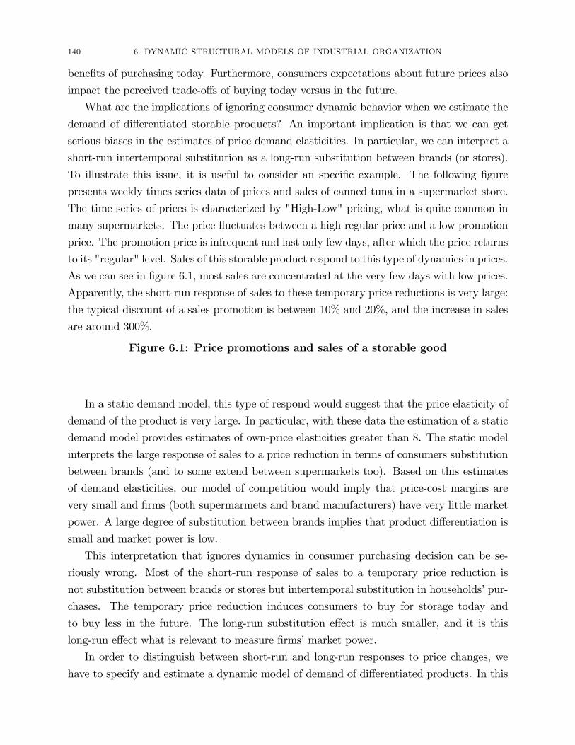
To illustrate this issue, it is useful to consider an speci�c example. The following �gure

presents weekly times series data of prices and sales of canned tuna in a supermarket store.

The time series of prices is characterized by "High-Low" pricing, what is quite common in

many supermarkets. The price �uctuates between a high regular price and a low promotion

price. The promotion price is infrequent and last only few days, after which the price returns

to its "regular" level. Sales of this storable product respond to this type of dynamics in prices.

As we can see in �gure 6.1, most sales are concentrated at the very few days with low prices.

Apparently, the short-run response of sales to these temporary price reductions is very large:

the typical discount of a sales promotion is between 10% and 20%, and the increase in sales

are around 300%.

Figure 6.1: Price promotions and sales of a storable good

In a static demand model, this type of respond would suggest that the price elasticity of

demand of the product is very large. In particular, with these data the estimation of a static

demand model provides estimates of own-price elasticities greater than 8. The static model

interprets the large response of sales to a price reduction in terms of consumers substitution

between brands (and to some extend between supermarkets too). Based on this estimates

of demand elasticities, our model of competition would imply that price-cost margins are

very small and �rms (both supermarmets and brand manufacturers) have very little market

power. A large degree of substitution between brands implies that product di¤erentiation is

small and market power is low.

This interpretation that ignores dynamics in consumer purchasing decision can be se-

riously wrong. Most of the short-run response of sales to a temporary price reduction is

not substitution between brands or stores but intertemporal substitution in households�pur-

chases. The temporary price reduction induces consumers to buy for storage today and

to buy less in the future. The long-run substitution e¤ect is much smaller, and it is this

long-run e¤ect what is relevant to measure �rms�market power.

In order to distinguish between short-run and long-run responses to price changes, we

have to specify and estimate a dynamic model of demand of di¤erentiated products. In this

1. INTRODUCTION 141

type of models consumers are forward looking and take into account their expectations about

future prices as well as storage costs.

1.2. Example 2: Demand of a new durable product. Melnikov (2000), Estebanand Shum (RAND, 2007), Carranza (2006), Gowrisankaran and Rysman (2009).

The price of new durable products typically declines over time during the months after the

introduction of the product. Figure 6.2 illustrates this point for the case of *****. Di¤erent

factors may explain this price decline, e.g., intertemporal price discrimination, increasing

competition, exogenous cost decline, or endogenous cost decline due to learning by doing.

As in the case of the "high-low" pricing of storable goods, explaining this pricing dynamics

also requires one to take into account dynamics in supply. For the moment, we concentrate

here in the demand. If consumers are forward looking, they expect the price will be lower

in the future and this generates an incentive to wait and buying the good in the future.

Figure 6.2: Price decline of new durable products

A static model that ignores dynamics in demand of durable goods can introduce two

di¤erent type of biases in the estimates of the distribution consumers willingness to pay

and therefore of demand. The �rst source of bias comes from the failure to recognize that

each period the potential market size is changing. Each period the demand curve is changing

because some high willingness-to-pay consumers have already bought the product and left the

market. A second source of bias comes from ignoring consumer forward-looking behavior. In

the static model, consumers willingness-to-pay can is contaminated by consumers�willingness

to wait because the expectation of future lower prices.

To illustrate the �rst source of bias, consider a market with an initial mass of 100 con-

sumers and a uniform distribution of willingness to pay over the the unit interval. To

concentrate on the �rst source of bias, consider that consumers are myopic and buy the

product if the price is below their willingness to pay. Once consumers buy the product they

are out of the market forever. Time is discrete and indexed by t 2 f1; 2; :::g. Every periodt, the aggregate demand is Qt = Ht Pr(vt � Pt) = Ht [1� Ft (Pt)], where Qt and Pt arequantity and price, respectively, Ht is the mass of consumers who remain in market at period

t, and Ft is the distribution function of willingness to pay for consumers who remain in the

market at period t. Suppose that we observe a sequence of prices equal to P1 = 0:9, P2 = 0:8,

P3 = 0:7, etc. Given this price sequence, it is easy to show that the demand curve at period

t = 1 is Q1 = 100(1 � P1), at period t = 2 the demand is Q2 = 90(0:9�P20:9) = 100(0:9 � P2),

at period t = 3 it is Q3 = 80(0:8�P30:8) = 100(0:8� P3), and so on. Therefore, the sequence of

quantities is constant over time: Q1 = Q2 = Q3 = ::: = 10. A static demand model lead the


researcher to conclude that consumers are not sensitive to price, since the same quantity is

sold as prices decline. The estimate of the price elasticity would be zero. This example but

it illustrates how ignoring dynamics in demand of durable goods can lead to serious biases

in the estimates of the price sensitivity of demand.

1.3. Example 3: Product repositioning in di¤erentiated product markets. Acommon assumption in many static (and dynamic) demand models of di¤erentiated prod-

ucts is that product characteristics, other than prices, are exogenous. However, in many

industries, product characteristics are very important strategic variables.

Ignoring the endogeneity of product characteristics has several implications. First, it

can biases in the estimated demand parameters. A dynamic game that acknowledges the

endogeneity of some product characteristics and exploits the dynamic structure of the model

to generate valid moment conditions can deal with this problem.

A second important limitation of a static model of �rm behavior is that it cannot recover

the costs of repositioning product characteristics. As a result, the static model cannot address

important empirical questions such as the e¤ect of a merger on product repositioning. That

is, the evaluation of the e¤ects of a merger using a static model should assume that the

product characteristics (other than prices) of the new merging �rm would remain the same

as before the merger. This is at odds both with the predictions of theoretical models and with

informal empirical evidence. Theoretical models of horizontal mergers show that product

repositioning is a potentially very important source of value for a merging �rm, and informal

empirical evidence shows that soon after a merger �rms implement signi�cant changes in

their product portfolio.

Sweeting (2007) and Aguirregabiria and Ho (2009) are two examples of empirical appli-

cations that endogenize product attributes using a dynamic game of competition in a dif-

ferentiated products industry. Sweeting estimates a dynamic game of oligopoly competition

in the US commercial radio industry. The model endogenizes the choice of radio stations

format (genre), and estimates product repositioning costs. Aguirregabiria and Ho (2009)

propose and estimate a dynamic game of airline network competition where the number of

direct connections that an airline has in an airport is an endogenous product characteristic.

1.4. Example 4: Dynamics of market structure. Ryan (2006) and Kasahara (JBES,2010) provide excellent examples of how ignoring supply-side dynamics and �rms�forward

looking behavior can lead to misleading results.

Ryan (2006) studies the e¤ects of the 1990 Amendments to the Clean Air Act on the US

cement industry. This environmental regulation added new categories of regulated emissions,

and introduced the requirement of an environmental certi�cation that cement plants have to

1. INTRODUCTION 143

pass before starting their operation. Ryan estimates a dynamic game of competition where

the sources of dynamics are sunk entry costs and adjustment costs associated with changes

in installed capacity. The estimated model shows that the new regulation had negligible

e¤ects on variable production costs but it increased signi�cantly the sunk cost of opening a

new cement plant. A static analysis, that ignores the e¤ects of the policy on �rms�entry-

exit decisions, would conclude that the regulation had negligible e¤ects on �rms pro�ts and

consumer welfare. In contrast, the dynamic analysis shows that the increase in sunk-entry

costs caused a reduction in the number of plants that in turn implied higher markups and a

decline in consumer welfare.

Kasahara (2010) proposes and estimates a dynamic model of �rm investment in equip-

ment and it uses the model to evaluate the e¤ect of an important increase in import tari¤s

in Chile during the 1980s. The increase in tari¤s had a substantial e¤ect of the price of

imported equipment and it may have a signi�cant e¤ect on �rms�investment. An important

feature of this policy is that the government announced that it was a temporary increase and

that tari¤s would go back to their original levels after few years. Kasahara shows that the

temporary aspect of this policy exacerbated its negative e¤ects on �rm investment. Given

that �rms anticipated the future decline in import tari¤s and the price of capital, a signif-

icant fraction of �rms decided not invest and waiting until the reduction of tari¤s. This

waiting and inaction would not appear if the policy change were perceived as permanent.

Kasahara shows that the Chilean economy would have recovered faster from the economic

crisis of 1982-83 if the increase in tari¤s would have been perceived as permanent.

1.5. Example 5: Dynamics of prices in a retail market. The signi�cant cross-sectional dispersion of prices is a well-known stylized fact in retail markets. Retailing �rms

selling the same product, and operating in the same (narrowly de�ned) geographic market

and at the same period of time, do charge prices that di¤er by signi�cant amounts, e.g., 10%

price di¤erentials or even larger. This empirical evidence has been well established for gas

stations and supermarkets, among other retail industries. Interestingly, the price di¤erentials

between �rms, and the ranking of �rms in terms prices, have very low persistence over time.

A gas station that charges a price 5% below the average in a given week may be charging a

price 5% above the average the next week. Using a more graphical description we can say

that a �rm�s price follows a cyclical pattern, and the price cycles of the di¤erent �rms in

the market are not synchronized. Understanding price dispersion and the dynamics of price

dispersion is very important to understand not only competition and market power but also

for the construction of price indexes.

Di¤erent explanations have been suggested to explain this empirical evidence. Some

explanations have to do with dynamic pricing behavior or "state dependence" in prices.


For instance, an explanation is based on the relationship between �rm inventory and

optimal price. In many retail industries with storable products, we observe that �rms�

orders to suppliers are infrequent. For instance, for products such as laundry detergent,

a supermarket ordering frequency can be lower than one order per month. A simple and

plausible explanation of this infrequency is that there are �xed or lump-sum costs of making

an order that do not depend on the size of the order, or at least they do not increase

proportionally with the size of the order. Then, inventories follow a so called (S,s) cycle: the

increase by a large amount up to a maximum when a place is order and then they decline

slowly up a minimum value where a new order is placed. Given this dynamics of inventories,

it is simple to show that optimal price of the �rm should also follow a cycle. The price drops

to a minimum when a new order is placed and then increases over time up to a maximum

just before the next order when the price drops again. Aguirregabiria (REStud, 1999) shows

this joint pattern of prices and inventories for many products in a supermarket chain. I show

that this type of inventory-depedence price dynamics can explain more than 20% of the time

series variability of prices in the data.

CHAPTER 7

Single-Agent Models of Firm Investment

1. Model and Assumptions

To present some common features of dynamic structural models, we start with a simple

model of �rm investment that we can represent as a machine replacement model.

Suppose that we have panel data of N plants operating in the same industry with infor-

mation on output, investment, and capital stock over T periods of time.

Data = f Yit, Iit, Kit : i = 1; 2; :::; N and t = 1; 2; :::; T g

Suppose that the investment data is characterized by infrequent and lumpy investments.

That is, Iit contains a large proportion of zeroes (no investment), and when investment is

positive the investment-to-capital ratio Iit=Kit is quite large. For instance, for some industries

and samples we can �nd that the proportion of zeroes is above 60% (even with annual data!)

and the average investment-to-capital ratio conditional on positive investment is above 50%.

A possible explanation for this type of dynamics in �rms�investment is that there are

signi�cant individibilities in the purchases of new capital, or/and �xed or lump-sum costs

associated with purchasing and installing new capital. Machine replacement models are

models of investment that emphasize the existence of these indivisibilities and lump-sum

costs of investment.

This type of investment models have been applied before in papers by Rust (Ectca, 1987),

Das (REStud, 1991), Kennet (RAND, 1994), Rust and Rothwell (JAE, 1995), Cooper, Halti-

wanger and Power (AER, 1999), Cooper and Haltiwanger (REStud 2006), and Kasahara

(JBES, 2010), among others. In Rust (1987) the �rm is a bus company (in Madison, Wis-

consin), a plant is a bus, and a machine is a bus engine. Das (1991) considers cement �rms

and a plant is a cement kiln. In Kennet (1994) studies airline companies and the machine is

an aircraft engine. Rust and Rothwell (1995) consider nuclear power plants. Cooper, Halti-

wanger and Power (1999), Cooper and Haltiwanger (2006), and Kasahara (2010) consider

manufacturing �rms and investment in equipment in general.

We index plants by i and time by t. A plant�s pro�t function is:

�it = Yit � Ct Iit �RCit145

146 7. SINGLE-AGENT MODELS OF FIRM INVESTMENT

Yit is the revenue of market value of the output produced by plant i at period t. Iit is

the amount of investment at period t. Ct is the price of new capital. And RCit represents

investment costs other than the cost of purchasing the new capital, i.e., costs of replacing

the old equipment (machine) by the new equipment.

Let Kit be the capital stock of plant i at the beginning of period t. As usual, capital

depreciates exogenously and it increases when new investments are made. This transition

rule of the capital stock is:

Kit+1 = (1� �) (Kit + Iit)

Following the key feature in models of machine replacement, we assume that there is an

indivisibility in the investment decision. In the standard machine replacement model, the

�rm decides between zero investment (Iit = 0) or the replacement of the old capital by a

"new machine" that implies a �xed amount of capital K�. Therefore,

Iit 2 f0 ; K� �Kit g

Therefore,

Kit+1 =

8<: (1� �) Kit if Iit = 0

(1� �) K� if Iit > 0or

Kit+1 = (1� �) [(1� ait) Kit + ait K�]

where ait is the indicator of positive investment, i.e., ait � 1fIit > 0g.This implies that the possible values of the capital stock are (1� �)K�, (1� �)2K�, etc.

Let Tit be the number of periods since the last machine replacement, i.e., time duration

since the last time that investment was positive. There is a one-to-one relationship between

capital Kit and the time duration Tit:

Kit = (1� �)Tit K�

or in logarithms, kit = k� � d Tit, where k� � logK� and d � � log(1� �) > 0.These assumptions on the values of investment and capital seem natural in applications

where the investment decision is actually a machine replacement decision, as in the papers

by Rust (1987), Das (1991), Kennet (1994), or Rust and Rothwell (1995), among others.

However, this framework may be restrictive when we look at less speci�c investment decisions,

such as investment in equipment as in the papers by Cooper, Haltiwanger and Power (1999),

Cooper and Haltiwanger (2006), and Kasahara (2010). In these other papers, investment

in the data is very lumpy, which is a prediction of a model of machine replacement, but

�rms in the sample have very di¤erent sizes (average over long periods of time) and their

capital stocks in those periods with positive investment are very di¤erent. These papers

consider that investment is either zero or a constant proportion of the installed capital, i.e.,

1. MODEL AND ASSUMPTIONS 147

Iit 2 f0 ; q Kitg where q is a constant, e.g., q = 25%. Here I maintained the most standardassumption of machine replacement models.

The production function (actually, revenue function) is:

Yit = exp��0 + �

Yi

[(1� ait) Kit + ait K

�]�1

where �0 and �1 are parameters, and �Yi captures productivity di¤erences between �rms

that are time-invariant. The speci�cation of the replacement cost function is:

RCit = ait ( r(Kit) + �Ci + "it )

r(K) is a function that is increasing in K, and �Ci and "it are zero mean random variables

that captures �rm heterogeneity in replacement costs. Therefore, the pro�t function is:

�it =

8<: exp��0 + �

Yi

K�1it if ait = 0

exp��0 + �

Yi

K��1 � Ct I� � r(Kit)� �Ci � "it if ait = 1

Every period t, the �rm observes the state variables Kit, Ct, and "it and then it decides

its investment in order to maximize its expected value:

Et

�X1

j=0�j �i;t+j

�where � 2 (0; 1) is the discount factor. The main trade-o¤ in this machine replacementdecision is simple. On the one hand, the productivity/e¢ ciency of a machine declines over

time and therefore the �rm prefers younger machines. However, using younger machines

requires frequent replacement and replacing a machine is costly.

The �rm has uncertainty about future realizations of Ct and "it. To complete the model

we have to specify the stochastic processes of these variables. We assume that Ct follows a

Markov process with transition probability fC(Ct+1jCt). For the shock in replacement costs"it we consider that it is i.i.d. with a logistic distribution with dispersion parameter �". The

individual e¤ects (�Yi ; �Ci ) have a �nite mixture distribution, i.e., (�

Yi ; �

Ci ) is a pair of random

variables from a distribution with discrete and �nite support F�.

Let Sit = (Kit, Ct, "it) be the vector of state variables in the decision problem of a plant

and let Vi(Sit) be the value function. This value function is the solution to the Bellmanequation:

Vi(Sit) = maxait2f0;1g

��i(ait; Sit) + �

ZVi(Sit+1) fS(Sit+1jait; Sit) dSit+1

�where fS(Sit+1jait; Sit) is the (conditional choice) transition probability of the state variables:

fS(Sit+1jait; Sit) = 1 fKit+1 = (1� �) [(1� ait) Kit + ait K�]g fC(Ct+1jCt) f"("it)

where 1f:g is the indicator function, and f" is the density function of "it.


We can also represent the Bellman equation as:

Vi(Sit) = max f vi(0;Kit; Ct) ; vi(1;Kit; Ct)� "it g

where vi(0;Kit; Ct) and vi(1;Kit; Ct) are the choice-speci�c value functions:

vi(0;Kit; Ct) � exp��0 + �

Yi

K�1it + �

ZVi((1� �)Kit; Ct+1; "it+1) fC(Ct+1jCt) df"("it)

vi(1;Kit; Ct) �exp

��0 + �

Yi

K�1it � Ct I� � r(Kit)� �Ci

+�

ZVi((1� �)K�; Ct+1; "it+1) fC(Ct+1jCt) df"("it)

2. Solving the dynamic programming (DP) problem

For given values of structural parameters and functions, f�0, �1, r(:), fC(:), �"g, andof the individual e¤ects �Yi and �

Ci , we can solve the DP problem of �rm i by simply using

successive approximations to the value function, i.e., iterations in the Bellman equation.

In models where some of the state variables are not serially correlated, it is computation-

ally very convenient (and also convenient for the estimation of the model) to de�ne versions

of the value function and the Bellman equation that are integrated over the non-serially

correlated variables. In our model, " is not serially correlated state variables. The integrated

value function of �rm i is:

�Vi(Kit; Ct) �ZVi(Kit; Ct; "it) df"("it)

And the integrated Bellman equation is:

�Vi(Kit; Ct) =

Zmax f vi(0;Kit; Ct) ; vi(1;Kit; Ct)� "it g df"("it)

The main advantage of using the integrated value function is that it has a lower dimen-

sionality than the original value function.

Given the extreme value distribution of "it, the integrated Bellman equation is:

�Vi(Kit; Ct) = �" ln

�exp

�vi(0;Kit; Ct)

�"

�+ exp

�vi(1;Kit; Ct)

�"

��where

vi(0;Kit; Ct) � exp��0 + �

Yi

K�1it + �

Z�Vi((1� �)Kit; Ct+1) fC(Ct+1jCt)

vi(1;Kit; Ct) � exp��0 + �

Yi

K�1it � Ct I� � r(Kit)� �Ci + �

Z�Vi((1� �)K�; Ct+1) fC(Ct+1jCt)

The optimal decision rule of this dynamic programming (DP) problem is:

ait = 1 f "it � vi(1;Kit; Ct)� vi(0;Kit; Ct) g

2. SOLVING THE DYNAMIC PROGRAMMING (DP) PROBLEM 149

Suppose that the price of new capital, Ct, has a discrete a �nite range of variation: Ct 2 fc1,c2, :::, cLg. Then, the value function �Vi can be represented as aM�1 vector in the Euclideanspace, where M = T � L and the T is the number of possible values for the capital stock.Let Vi be that vector. The integrated Bellman equation in matrix form is:

Vi = �" ln

�exp

��i(0) + � F(0) Vi

�"

�+ exp

��i(1) + � F(1) Vi

�"

��where �i(0) and �i(1) are the M � 1 vectors of one-period pro�ts when ait = 0 and ait = 1,respectively. F(0) and F(0) areM�M transition probability matrices of (Kit; Ct) conditional

on ait = 0 and ait = 1, respectively.

Given this equation, the vector Vi can be obtained by using value function iterations in

the Bellman equation. Let V0i be an arbitrary initial value for the vector Vi. For instance,

V0i could be a M � 1 vector of zeroes. Then, at iteration k = 1; 2; ::: we obtain:

Vki = �" ln

�exp

��i(0) + � F(0) V

k�1i

�"

�+ exp

��i(1) + � F(1) V

k�1i

�"

��Since the (integrated) Bellman equation is a contraction mapping, this algorithm always

converges (regardless the initial V0i ) and it converges to the unique �xed point. Exact

convergence requires in�nite iterations. Therefore, we stop the algorithm when the distance

(e.g., Euclidean distance) between Vki and V

k�1i is smaller than some small constant, e.g.,

10�6.

An alternative algorithm to solve the DP problem is the Policy Iteration algorithm.De�ne the Conditional Choice Probability (CCP) function Pi(Kit; Ct) as:

Pi(Kit; Ct) � Pr ( "it � vi(1;Kit; Ct)� vi(0;Kit; Ct) )

=

exp

�vi(1;Kit; Ct)� vi(0;Kit; Ct)

�"

�1 + exp

�vi(1;Kit; Ct)� vi(0;Kit; Ct)

�"

�Given that (Kit; Ct) are discrete variables, we can describe the CCP function Pi(:) as aM�1vector of probabilities Pi. The expression for the CCP in vector form is:

Pi =

exp

��i(1)��i(0) + � [F(1)� F(0)] Vi

�"

�1 + exp

��i(1)��i(0) + � [F(1)� F(0)] Vi

�"

�

Suppose that the �rm behaves according to the probs in Pi. Let VPi the vector of values

if the �rm behaves according to P. That is VPi is the expected discounted sum of current


and future pro�ts if the �rm behaves according to Pi. Ignoring for the moment the expected

future "0s, we have that:

VPi = (1�Pi) �

��i(0) + � F(0)V

Pi

�+Pi �

��i(1) + � F(1)V

Pi

�And solving for VP

i :

VPi =

�I � � FPi

��1((1�Pi) ��i(0) +Pi ��i(1))

where FPi = (1�Pi) � F(0) +Pi � F(1).Taking into account this expression for VP

i , we have that the optimal CCP Pi is such

that:

Pi =

exp

(~�i + � ~F

�I � � FPi

��1((1�Pi) ��i(0) +Pi ��i(1))

�"

)

1 + exp

(~�i + � ~F

�I � � FPi

��1((1�Pi) ��i(0) +Pi ��i(1))

�"

)

where ~�i � �i(1)��i(0), and ~F � F(1)�F(0). This equation de�nes a �xed point mappingin Pi. This �xed point mapping is called the Policy Iteration mapping. This is also a

contraction mapping. Optimal Pi is its unique �xed point.

Therefore we compute Pi by iterating in this mapping. Let P0i be an arbitrary initial

value for the vector Pi. For instance, P0i could be a M � 1 vector of zeroes. Then, at eachiteration k = 1; 2; ::: we do "two things":

Valuation step:

Vki =

�I � � FP

k�1i

��1 �(1�Pk�1i ) ��i(0) +P

k�1i ��i(1)

�Policy step:

Pki =

exp

(~�i + � ~F V

ki

�"

)

1 + exp

(~�i + � ~F V

ki

�"

)Policy iterations are more costly than Value function iterations (especially because the

matrix inversion in the valuation step). However, the policy iteration algorithm requires

a much lower number of iterations, especially with � is close to one. Rust (1987, 1994)

proposes an hybrid algorithm: start with a few value function iterations and then switch to

policy iterations.

3. ESTIMATION 151

3. Estimation

The primitives of the model are: (a) The parameters in the production function; (b) the

replacement costs function r(:); (c) the probability distribution of �rm heterogeneity F�(:);

(d) the dispersion parameter �"; and (e) the discount factor �. Let � represent the vector of

structural parameters. We are interested in the estimation of �.

Here I describe the Maximum Likelihood estimation of these parameters. Conditional on

the observe history of price of capital and on the initial condition for the capital stock, we

have that:

Pr (Data j C, Ki1, �) =NYi=1

Pr (ai1,Yi1; ...; aiT ,YiT j C, Ki1, �)

The probability Pr (ai1,Yi1; ...; aiT ,YiT j C, Ki1, �) is the contribution of �rm i to the likeli-

hood function. Conditional on the individual heterogeneity, �i � (�Yi ; �Ci ), we have that:

Pr (ai1,Yi1; ...; aiT ,YiT j C, Ki1, �i, �) =TYt=1

Pr (ait,Yit j Ct, Kit, �i, �)

=TYt=1

Pr (Yit j ait, Ct, Kit, �i, �) Pr (ait j Ct, Kit, �i, �)

where Pr (ait j Ct, Kit, �i, �) is the CCP function:

Pr (ait j Ct, Kit, �i, �) = Pi (Kit; Ct, �)ait [1� Pi (Kit; Ct, �)]

1�ait

and Pr (Yit j ait, Ct, Kit, �i, �) comes from the production function, Yit = exp��0 + �

Yi

[(1� ait) Kit + ait K

�]�1. In logarithms, the production function is:

lnYit = �0 + �1 (1� ait) lnKit + � ait + �Yi + eit

where � is a parameter that represents �1 lnK�, and eit is a measurement error in output,

that we assume i.i.d. N(0; �2e) and independent of "it. Therefore,

Pr (Yit j ait, Ct, Kit, �i, �) = �

�lnYit � �0 � �1 (1� ait) lnKit � � ait � �Yi

�e

�where � (:) is the PDF of the standard normal distribution.

Putting all these pieces together, we have that the log-likelihood function of the model

is `(�) =PN

i=1 lnLi(�) where Li(�) � Pr (ai1,Yi1; ...; aiT ,YiT j C, Ki1, �) and:

Li(�) =P�2

F�(�)

26664TYt=1

�

�lnYit � �0 � �1 (1� ait) lnKit � � ait � �Y

�e

�

Pi (Kit; Ct, �, �)ait [1� Pi (Kit; Ct, �, �)]

1�ait

37775Given this likelihood, we can estimate by Maximum Likelihood (ML)


The NFXP algorithm is a gradient iterative search method to obtain the MLE of the

structural parameters.

This algorithm nests a BHHH method (outer algorithm), that searches for a root of the

likelihood equations, with a value function or policy iteration method (inner algorithm), that

solves the DP problem for each trial value of the structural parameters. The algorithm is

initialized with an arbitrary vector �̂0.

A BHHH iteration is de�ned as:

�̂k+1 = �̂k +

NXi=1

Oli(�̂k)Oli(�̂k)0!�1 NX

i=1

Oli(�̂k)!

where Oli(�) is the gradient in � of the log-likelihood function for individual i. In a partiallikelihood context, the score Oli(�) is:

Oli(�) =TiXt=1

O logP (aitjxit;�)

To obtain this score we have to solve the DP problem.

In our machine replacement model:

l(�) =NXi=1

TiXt=1

ait logP (xit; �) + (1� ait) log(1� P (xit; �))

with:

P(�) = F~"

�[�Y 0 + �Y 1X+ � Fx(0)V(�)]

� [�Y 0 � �R0 � �Y 1X+ � Fx(1)V(�)]

�

The NFXP algorithm works as follows. At each iteration we can distinguish three main

tasks or steps.

Step 1: Inner iteration: DP solution. Given �̂0, we obtain the vector�V(�̂0) by using either successive iterations or policy iterations.

Step 2: Construction of scores. Then, given �̂0 and �V(�̂0) we constructthe choice probabilities

P(�̂0) = F~"

0@ h�Y 0 + �Y 1X+ � Fx(0)V(�̂0)

i�h�Y 0 � �R0 � �Y 1X+ � Fx(1)V(�̂0)

i 1Athe Jacobian

@ �V(�̂0)0

@�and the scores Oli(�̂0)

Step 3: BHHH iteration. We we use the scores Oli(�̂0) to make a newBHHH iteration to obtain �̂1.

�̂1 = �̂0 +

NXi=1

Oli(�̂0)Oli(�̂0)0!

NXi=1

Oli(�̂0)!

4. PATENT RENEWAL MODELS 153

Then, we replace �̂0 by �̂1 and go back to step 1.

* We repeat stesp 1 to 3 until convergence: i.e., until the distance between �̂1and �̂0 is smaller than a pre-speci�ed convergence constant.

The main advantages of the NFXP algorithm are its conceptual simplicity and, more

importantly, that it provides the MLE which is the most e¢ cient estimator asymptotically

under the assumptions of the model.

The main limitation of this algorithm is its computational cost. In particular, the DP

problem should be solved for each trial value of the structural parameters.

4. Patent Renewal Models

�What is the value of a patent? How to measure it?� The valuation of patents is very important for: merger & acquisition decisions; using

patents as collateral for loans; value of innovations; value of patent protection.

� Very few patents are traded, and there is substantial selection. We cannot use an "hedonic"approach.

� The number of citations of a patent is a very imperfect measure of patent value.� Multiple patents are used in the production of multiple products, and in generating newpatents. A "production function approach" seems also unfeasible.

� Pakes (1986) proposes using information on patent renewal fees together with a RevealPreference approach to estimate the value of a patent.

� Every year, a patent holder should pay a renewal fee to keep her patent.� If the patent holder decides to renew, it is because her expected value of holding the patentis greater than the renewal fee (that is publicly known).

� Therefore, observed decisions on patent renewal / non renewal contain information on thevalue of a patent.

Model: Basic Framework

� Consider a patent holder who has to decide whether to renew her patent or not. We indexpatents by i.

� This decision should be taken at ages t = 1; 2; :::; T where T <1 is the regulated term of

a patent (e.g., 20 years in US, Europe, or Canada).

� Patent regulation also establishes a sequence of Maintenance Fees fct : t = 1; 2; :::; Tg.This sequence of renewal fees is deterministic such that a patent owner knows with certainty

future renewal fees.


� The schedule fct : t = 1; 2; :::; Tg is typically increasing in patent age t and it may godfrom a few hundred dollars to a few thousand dollars.

� A patent generates a sequence of pro�ts f�it : t = 1; 2; :::; Tg.� At age t, a patent holder knows current pro�t �it but has uncertainty about future pro�ts�i;t+1, �i;t+2, ...

� The evolution of pro�ts depends on the following factors:(1) the initial "quality" of the idea/patent;

(2) innovations (new patents) which are substitutes of the patent and therefore, depreciate

its value or even make it obsolete;

(3) innovations (new patents) which are complements of the patent and therefore, increase

its value.

Stochastic process of patent pro�ts

� Pakes proposes the following stochastic process for pro�ts, that tries to capture the threeforces mentioned above.

� A patent pro�t at the �rst period is a random draw from a log-normal distribution with

parameters �1 and �1:

ln(�i1) � N(�1; �21)� After the �rst year, pro�t evolves according to the following formula:

�i;t+1 = � i;t+1 max�� it ; �i;t+1

� � 2 (0; 1) is the depreciation rate. In the absence of unexpected shocks, the value of thepatent depreciates according to the rule: �i;t+1 = � �it.

� � i;t+1 2 f0; 1g is a binary variable that represents that the patent becomes obsolete (i.e.,zero value) due to competing innovations. The probability of this event is a decreasing

function of pro�t at previous year:

Pr(� i;t+1 = 0 j �it; t) = expf�� itg

� The largest is the pro�t of the patent at age t, the smallest is the probability that itbecomes obsolete.

� Variable �i;t+1 represents innovations which are complements of the patent and increase itspro�tability.

� �i;t+1 has an exponential distribution with mean and standard deviation �t�:

p(�i;t+1 j �it; t) =1

�t�exp

�� + �i;t+1

�t�

�� If � < 1, the variance of �i;t+1 declines over time (and the E(max

�x ; �i;t+1

) value

declines as well).


� If � > 1, the variance of �i;t+1 increases over time (and the E(max�x ; �i;t+1

) value

increases as well).

� Under this speci�cation, pro�ts f�itg follow a non-homogeneous Markov process with initialdensity �i1 � lnN(�1; �21), and transition density function:

f" (�it+1j�it; t) =

8>>>>>><>>>>>>:

expf�� itg if �it+1 = 0

Pr��it+1 < ��it j �it; t

�if �it+1 = ��it

1

�t�exp

�� + �it+1

�t�

�if �it+1 > ��it

� The vector of structural parameters is � = (�; �; ; �; �; �1; �1).

Model: Dynamic Decision Model

� Vt(�) is the value of an active patent of age t and current pro�t �.� Let ait 2 f0; 1g be the decision variable that represents the event "the patent owner decidesto renew the patent at age t".

� The value function is implicitly de�ned by the Bellman equation:

Vt(�it) = max

�0 ; �it � ct + �

ZVt+1(�i;t+1) f"(d�i;t+1 j �it; t)

�with Vt(�it) = 0 for any t � T + 1.� The value of not renewal (ait = 0) is zero. The value of renewal (ait = 1) is the currentpro�t �it � ct plus the expected and discounted future value.

Model: Solution (Backwards induction)

� We can use backwards induction to solve for the sequence of value functions fVtg andoptimal decision rules f�tg:� Starting at age t = T , for any pro�t �:

VT (�) = max f 0 ; � � cTg

and

�T (�) = 1 f � � cT � 0 g

� Then, for age t < T , and for any pro�t �:

Vt(�) = max

�0 ; � � ct + �

ZVt+1(�

0) f"(d�0j�; t)

�and

�t(�) = 1

�� ct + �

ZVt+1(�

0) f"(d�0j�; t) � 0

�Solution - A useful result


� Given the form of f"(�0j�; t), the future and discounted expected value, �RVt+1(�

0)

f"(d�0j�; t), is increasing in current �.

� This implies that the solution of the DP problem can be described as a sequence ofthreshold values for pro�ts f��t : t = 1; 2; :::; Tg such that the optimal decision rule is:

�t(�) = 1 f � � ��t g

� ��t is the level of current pro�ts that leaves the owner indi¤erent between renewing thepatent or not: Vt(��t ) = 0.

� These threshold values are obtained using backwards induction:� At period t = T :

��T = cT

� At period t < T , ��t is the unique solution to the equation:

��t � ct + E

TXs=t+1

�s�t maxf 0 ; �t+1 � ��t+1 g j �t = ��t

!= 0

� Solving for a sequence of threshold values is much simpler that solving for a sequence ofvalue functions.

Data

� Sample of N patents with complete (uncensored) durations fdi : i = 1; 2; :::Ng, wheredi 2 f1; 2; :::; T + 1g is patent i�s duration or age at its last renewal period.� The information in this sample can be summarized by the empirical distribution of fdig:

bp(t) = 1

N

NXi=1

1fdi = tg

Estimation: Likelihood

� The log-likelihood function of this model and data is:

l(�) =

NXi=1

T+1Xt=1

1fdi = tg ln Pr(di = tj�)

= N

T+1Xt=1

bp(t) lnP (tj�)


where:P (tj�) = Pr (�s � ��s for s � t� 1,and �t < ��t j �)

=

1Z��1

:::

1Z��t�1

��tZ0

dF (�1; :::; �t�1; �t)

� Computing P (tj�) involves solving an integral of dimension t. For t greater than 4 or 5, itis computationally very costly to obtain the exact value of these probabilities. Instead, we

approximate these probabilities using Monte Carlo simulation.

Estimation: Simulation of Probabilities

� For a given value of �, let f�simt (�) : t = 1; 2; :::; Tg be a simulated history of pro�ts forpatent i.

� Suppose that, for a given value of �, we simulate R independent pro�t histories. Letf�simrt (�) : t = 1; 2; :::; T ; r = 1; 2; :::; Rg be these histories.� Then, we can approximate the probability P (tj�) using the following simulator:

~PR(tj�) =1

R

RXr=1

1f�simrs (�) � ��s for s � t� 1,and �simrt < ��tg

� ~PR(tj�) is a raw frequency simulator. It has the following properties (Note that these areproperties of a simulator, not of an estimator. ~PR(tj�) does not depend on the data).(1) Unbiased: E

�~PR(tj�)

�= P (tj�)

(2) V ar( ~PR(tj�)) = P (tj�)(1� P (tj�))=R(3) Consistent as R!1.

� It is possible to obtain better simulators (with lower variance) by using importance-sampling simulation. This is relevant because the bias and variance of simulated-based

estimators depend on the variance (and bias) of the simulator.

� Furthermore, when P (tj�) is small, the simulator ~PR(tj�) can be zero even when R is large,and this creates problems for ML estimation.

� A simple solution to this problem is to consider the following simulator which is based on

the raw-frequency simulated probabilities ~PR(1j�), ~PR(2j�), .... ~PR(T + 1j�):

P �R(tj�) =exp

(~PR(tj�)�

)XT+1

s=1exp

(~PR(sj�)�

)where � > 0 is an smoothing parameter.


� The simulator P �R is biased. However, if � ! 0 as R ! 1, then P �R is consistent, it haslower variance than ~PR, and it is always strictly positive.

Simulation-Based Estimation

� The estimator of � (Simulated Method of Moments estimator) is the value that solves thesystem of T equations: for t = 1; 2; :::T :

1

N

NXi=1

h1fdi = tg � ~PR;i(tj�)

i= 0

where the subindex i in the simulator ~PR;i(tj�) indicates that for each patent i in the samplewe draw R independent histories and compute independent simulators.

� E¤ect of simulation error. Note that ~PR;i(tj�) is unbiased such that ~PR;i(tj�) = P (tj�)+ei(t; �), where ei(t; �) is the simulation error. Since the simulation errors are independent

random draws:

1

N

NXi=1

ei(t; �)!p 0 and1pN

NXi=1

ei(t; �)!d N(0; VR)

The estimator is consistent an asymptotically normal for any R. The variance of the esti-

mator declines with R.

Identi�cation

� Since there are only 20 di¤erent values for the renewal fees fctg we can at most identify20 di¤erent points in the probability distribution of patent values.

� The estimated distribution at other points is the result of interpolation or extrapolationbased on the functional form assumptions on the stochastic process for pro�ts.

� It is important to note that the identi�cation of the distribution of patent values is NOTup to scale but in dollar values.

� For a given patent of with age t, all what we can say is that: if ait = 0 , then Vit < V (��t );and if ait = 1 , then Vit � V (��t ).

Empirical Questions

� The estimated model can be used to address important empirical questions.� Valuation of the stock of patents. Pakes uses the estimated model to obtain the valueof the stock of patents in a country.

� According to the estimated model, the value of the stock of patents in 1963 was $315million in France, $385 million in UK, and $511 in Germany.

� Combining these �gures with data on R&D investments in these countries, Pakes calculatesrates of return of 15.6%, 11.0% and 13.8%, which look like quite reasonable.

5. DYNAMIC STRUCTURAL MODELS OF TEMPORARY SALES AND INVENTORIES 159

Empirical Questions

� Factual policies. The estimated model shows that a very important part of the observedbetween-country di¤erences in patent renewal can be explained by di¤erences in policy pa-

rameters (i.e., renewal fees and maximum length).

� Counterfactual policy experiments. The estimated model can be used to evaluate thee¤ects of policy changes (in renewal fees and/or in maximum length) which are not observed

in the data.

5. Dynamic structural models of temporary sales and inventories

Recent empirical papers show that temporary sales account for approximately half of all

price changes of retail products in US (Hosken and Rei¤en, 2004, Nakamura and Steinsson,

2008, Midrigan, 2011). Understanding the determinants of temporary sales is important to

understand price stickiness and price dispersion, and it has important implications on the

e¤ects of monetary policy. It has also important implications in the study of �rms�market

power and competition.

Here I describe three di¤erent models of sales promotions based on the papers by Slade

(1998), Aguirregabiria (1999), Pesendorfer (2002), and Kano (2013).

5.1. Slade (1998).

5.2. Aguirregabiria (1999). � The signi�cant cross-sectional dispersion of prices isa well-known stylized fact in retail markets. Retailing �rms selling the same product, and

operating in the same (narrowly de�ned) geographic market and at the same period of time,

do charge prices that di¤er by signi�cant amounts, e.g., 10% price di¤erentials or even larger.

This empirical evidence has been well established for gas stations and supermarkets, among

other retail industries. Interestingly, the price di¤erentials between �rms, and the ranking

of �rms in terms prices, have very low persistence over time. A gas station that charges a

price 5% below the average in a given week may be charging a price 5% above the average

the next week. Using a more graphical description we can say that a �rm�s price follows a

cyclical pattern, and the price cycles of the di¤erent �rms in the market are not synchronized.

Understanding price dispersion and the dynamics of price dispersion is very important to

understand not only competition and market power but also for the construction of price

indexes.

� Di¤erent explanations have been suggested to explain this empirical evidence. Some ex-planations have to do with dynamic pricing behavior or "state dependence" in prices.


� For instance, an explanation is based on the relationship between �rm inventory and

optimal price. In many retail industries with storable products, we observe that �rms�

orders to suppliers are infrequent. For instance, for products such as laundry detergent,

a supermarket ordering frequency can be lower than one order per month. A simple and

plausible explanation of this infrequency is that there are �xed or lump-sum costs of making

an order that do not depend on the size of the order, or at least they do not increase

proportionally with the size of the order. Then, inventories follow a so called (S,s) cycle: the

increase by a large amount up to a maximum when a place is order and then they decline

slowly up a minimum value where a new order is placed. Given this dynamics of inventories,

it is simple to show that optimal price of the �rm should also follow a cycle. The price drops

to a minimum when a new order is placed and then increases over time up to a maximum

just before the next order when the price drops again. Aguirregabiria (REStud, 1999) shows

this joint pattern of prices and inventories for many products in a supermarket chain. I show

that this type of inventory-depedence price dynamics can explain more than 20% of the time

series variability of prices in the data.

Temporary sales and inventories

� Recent empirical papers show that temporary sales account for approximately half of allprice changes of retail products in US: Hosken and Rei¤en (RAND, 2004); Nakamura and

Steinsson (QJE, 2008); Midrigan (Econometrica, 2011).

� Understanding the determinants of temporary sales is important to understand price sticki-ness and price dispersion, and it has important implications on the e¤ects of monetary policy.

� It has also important implications in the study of �rms�market power and competition.� Di¤erent empirical models of sales promotions: Slade (1998) [Endogenous consumer loy-alty], Aguirregabiria (1999) [Inventories], Pesendorfer (2002) [Intertemporal price discrimi-

nation], and Kano (2013).

� This paper studies how retail inventories, and in particular (S,s) inventory behavior, canexplain both price dispersion and sales promotions in retail markets.

� Three factors are key for the explanation provided in this paper:(1) Fixed (lump-sum) ordering costs, that generates (S,s) inventory behavior.

(2) Demand uncertainty.

(3) Sticky prices (Menu costs) that, together with demand uncertainty, creates a

positive probability of excess demand (stockout).

Model: Basic framework

� Consider a retail �rm selling a product. We index products by i.


� Every period (month) t the �rm decides the retail price and the quantity of the product

to order to manufacturers/wholesalers

�Monthly sales are the minimum of supply an demand:

yit = min f dit ; sit + qit g

� yit = sales in physical units� dit = demand� sit = inventories at the beginning of month t� qit = orders (and deliveries) during month t

Demand and Expected sales

� The �rm has uncertainty about current demand:

dit = deit exp (�it)

� deit = expected demand� �it = zero mean demand shock unknown to the �rm at t.

� Therefore, expected sales are:

yeit =

Zmin fdeit exp (�) ; sit + qit g dF�(�)

� Assume monopolistic competition. Expected Demand depends on the own price, pit,and a demand shock !it. The functional form is isoelastic:

deit = exp f 0 � 1 ln(pit) + !it g

where 0 and 1 > 0 are parameters.

Price elasticity of expected sales

� Demand uncertainty has important implications for the relationship between prices andinventories.

� The price elasticity of expected sales is a function of the supply-to-expected-demandratio (sit + qit)=deit:

�yejp ��@ye@p

p

ye= �

�RI fde exp (�) ; s+ q g dF�(�)

� @de@p

p

ye

= 1 F�

�log

�s+ q

de

��de

ye

� And we have that:

�yejp �!

8<: 1 as (s+ q)=de �!1

0 as (s+ q)=de �! 0

Price elasticity of expected sales


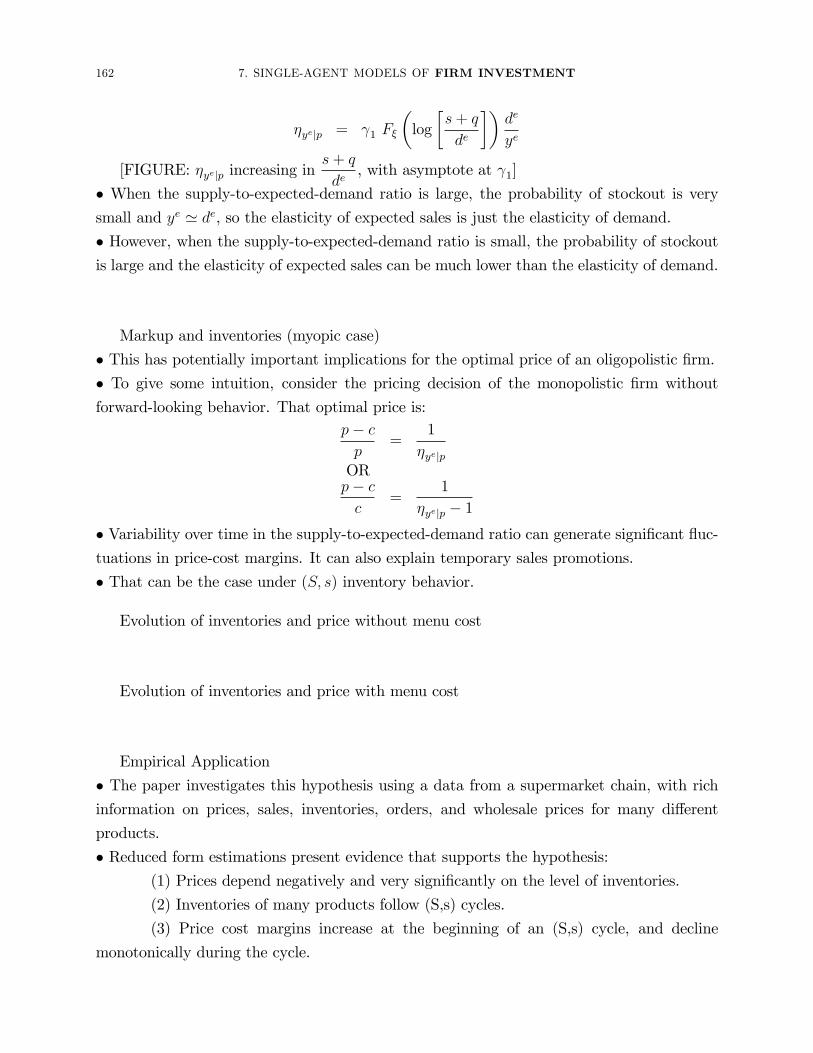
�yejp = 1 F�

�log

�s+ q

de

��de

ye

[FIGURE: �yejp increasing ins+ q

de, with asymptote at 1]

� When the supply-to-expected-demand ratio is large, the probability of stockout is verysmall and ye ' de, so the elasticity of expected sales is just the elasticity of demand.� However, when the supply-to-expected-demand ratio is small, the probability of stockoutis large and the elasticity of expected sales can be much lower than the elasticity of demand.

Markup and inventories (myopic case)

� This has potentially important implications for the optimal price of an oligopolistic �rm.� To give some intuition, consider the pricing decision of the monopolistic �rm without

forward-looking behavior. That optimal price is:p� cp

=1

�yejpORp� cc

=1

�yejp � 1� Variability over time in the supply-to-expected-demand ratio can generate signi�cant �uc-tuations in price-cost margins. It can also explain temporary sales promotions.

� That can be the case under (S; s) inventory behavior.

Evolution of inventories and price without menu cost

Evolution of inventories and price with menu cost

Empirical Application

� The paper investigates this hypothesis using a data from a supermarket chain, with rich

information on prices, sales, inventories, orders, and wholesale prices for many di¤erent

products.

� Reduced form estimations present evidence that supports the hypothesis:

(1) Prices depend negatively and very signi�cantly on the level of inventories.

(2) Inventories of many products follow (S,s) cycles.

(3) Price cost margins increase at the beginning of an (S,s) cycle, and decline

monotonically during the cycle.


� I estimate the parameters in the pro�t function (demand parameters, ordering costs, in-ventory holding costs) and use the estimated model to analyze how much of price variation

and temporary sales promotions can be explained by �rm inventories.

Pro�t function

� Expected current pro�ts are equal to expected revenue, minus ordering costs, inventoryholding costs and price adjustment costs:

�it = pit yeit �OCit � ICit � PACit

� OCit = ordering costs� ICit = inventory holding costs� PACit = price adjustment (menu) costs

� Ordering costs:

OCit =

8<: 0 if qit = 0

Foc + "ocit � cit qit if qit > 0

� Foc = �xed (lump-sum) ordering cost. Parameter.� "ocit = zero mean shock in the �xed ordering cost.� cit = wholesale price

� Inventory holding costs:

ICit = � sit

�Menu costs:

PACit =

8>>>><>>>>:0 if pit = pi;t�1

F(+)mc + "

mc(+)it if pit > pi;t�1

F(�)mc + "

mc(�)it if pit < pi;t�1

� F (+)mc and F(�)mc are price adjustment cost parameters

� "mc(+)it and "mc(�)it are zero mean shocks in menu costs

State variables

� The state variables of this DP problem are:8<:sit, cit, pi;t�1, !it| {z }xit

, "ocit , "mc(+)it , "mc(+)it| {z }

"it

9=;� The decision variables are qit and �pit � pit � pi;t�1. We use ait to denote (qit,�pit).


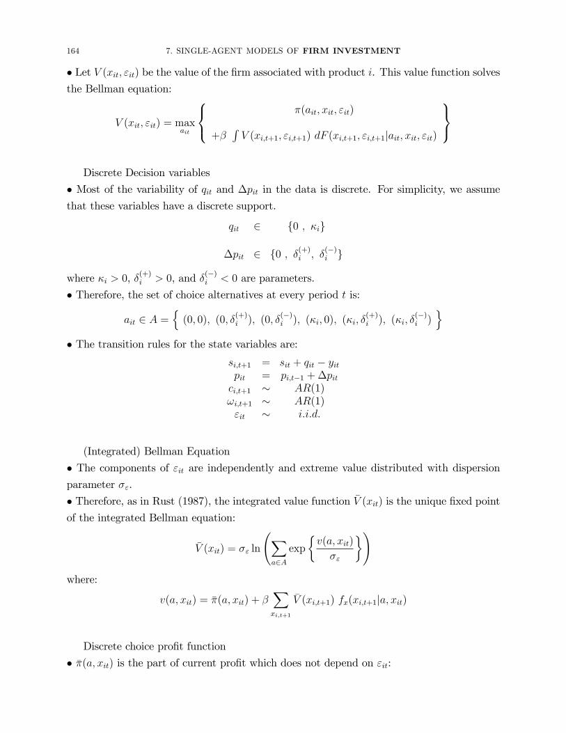
� Let V (xit; "it) be the value of the �rm associated with product i. This value function solvesthe Bellman equation:

V (xit; "it) = maxait

8<: �(ait; xit; "it)

+�RV (xi;t+1; "i;t+1) dF (xi;t+1; "i;t+1jait; xit; "it)

9=;Discrete Decision variables

� Most of the variability of qit and �pit in the data is discrete. For simplicity, we assumethat these variables have a discrete support.

qit 2 f0 ; �ig

�pit 2 f0 ; �(+)i ; �(�)i g

where �i > 0, �(+)i > 0, and �(�)i < 0 are parameters.

� Therefore, the set of choice alternatives at every period t is:

ait 2 A =n(0; 0); (0; �

(+)i ); (0; �

(�)i ); (�i; 0); (�i; �

(+)i ); (�i; �

(�)i )

o� The transition rules for the state variables are:

si;t+1 = sit + qit � yitpit = pi;t�1 +�pitci;t+1 � AR(1)!i;t+1 � AR(1)"it � i:i:d:

(Integrated) Bellman Equation

� The components of "it are independently and extreme value distributed with dispersionparameter �".

� Therefore, as in Rust (1987), the integrated value function �V (xit) is the unique �xed pointof the integrated Bellman equation:

�V (xit) = �" ln

Xa2A

exp

�v(a; xit)

�"

�!where:

v(a; xit) = ��(a; xit) + �Xxi;t+1

�V (xi;t+1) fx(xi;t+1ja; xit)

Discrete choice pro�t function

� ��(a; xit) is the part of current pro�t which does not depend on "it:


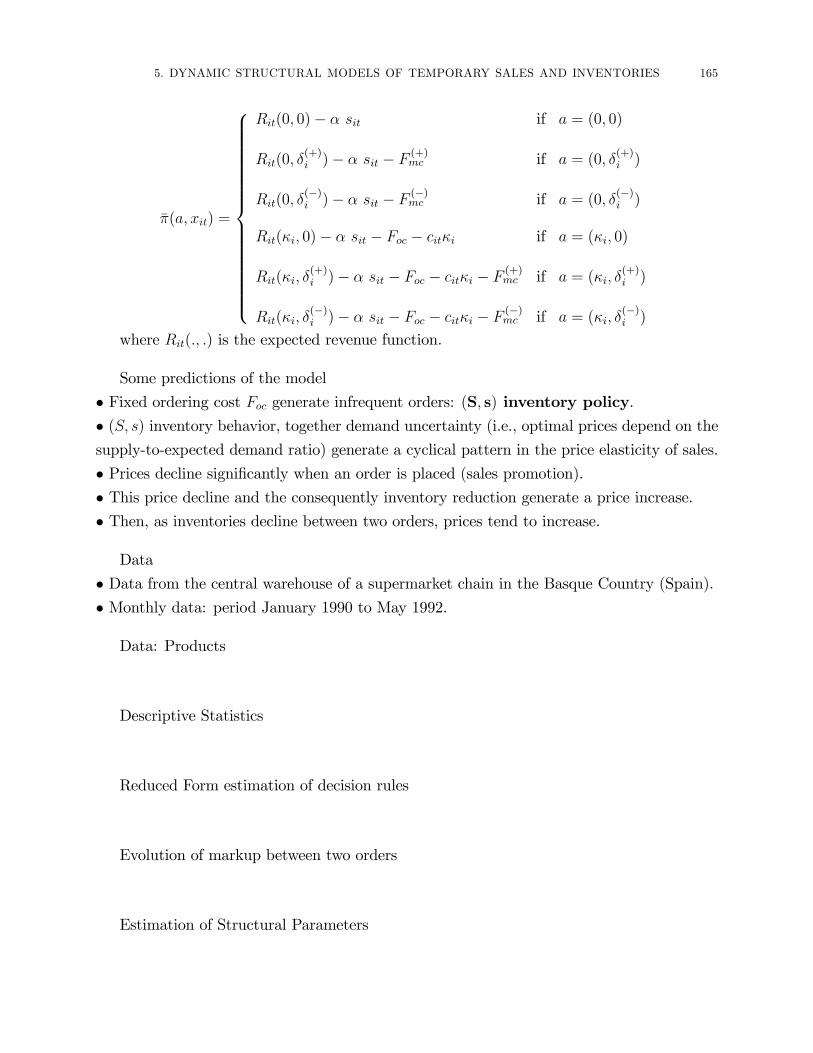
��(a; xit) =

8>>>>>>>>>>>>>>>><>>>>>>>>>>>>>>>>:

Rit(0; 0)� � sit if a = (0; 0)

Rit(0; �(+)i )� � sit � F (+)mc if a = (0; �

(+)i )

Rit(0; �(�)i )� � sit � F (�)mc if a = (0; �

(�)i )

Rit(�i; 0)� � sit � Foc � cit�i if a = (�i; 0)

Rit(�i; �(+)i )� � sit � Foc � cit�i � F (+)mc if a = (�i; �

(+)i )

Rit(�i; �(�)i )� � sit � Foc � cit�i � F (�)mc if a = (�i; �

(�)i )

where Rit(:; :) is the expected revenue function.

Some predictions of the model

� Fixed ordering cost Foc generate infrequent orders: (S; s) inventory policy.� (S; s) inventory behavior, together demand uncertainty (i.e., optimal prices depend on thesupply-to-expected demand ratio) generate a cyclical pattern in the price elasticity of sales.

� Prices decline signi�cantly when an order is placed (sales promotion).� This price decline and the consequently inventory reduction generate a price increase.� Then, as inventories decline between two orders, prices tend to increase.

Data

� Data from the central warehouse of a supermarket chain in the Basque Country (Spain).

� Monthly data: period January 1990 to May 1992.

Data: Products

Descriptive Statistics

Reduced Form estimation of decision rules

Evolution of markup between two orders

Estimation of Structural Parameters


Counterfactual Experiments

5.3. Pesendorfer (2002).

5.4. Kano (2013).

CHAPTER 8

Structural Models of Dynamic Demand of Di¤erentiated Products

1. Introduction

Consumers can stockpile a storable good when prices are low and use the stock for future

consumption. This stockpiling behavior can introduce signi�cant di¤erences between short-

run and long-run responses of demand to price changes. Also, the response of demand to

a price change depends on consumers�expectations/beliefs about how permanent the price

change is. For instance, if a price reduction is perceived by consumers as very transitory

(e.g., a sales promotion), then a signi�cant proportion of consumers may choose to increase

purchases today, stockpile the product and reduce their purchases during future periods when

the price will be higher. If the price reduction is perceived as permanent, this intertemporal

substitution of consumer purchases will be much lower or even zero.

Ignoring consumers�stockpiling and forward-looking behavior can introduce serious biases

in estimated own- and cross- price demand elasticities. These biases can be particularly

serious when the time series of prices is characterized by "High-Low" pricing. The price

�uctuates between a (high) regular price and a (low) promotion price. The promotion price

is infrequent and last only few days, after which the price returns to its "regular" level. Most

sales are concentrated in the very few days of promotion prices.

Pesendorfer (Journal of Business, 2002)

Static demand models assume that all the substitution is either between brands or prod-

uct expansion. They rule out intertemporal substitution. This can imply serious biases in

the estimated demand elasticities. With High-Low pricing, we expect the static model to

over-estimate the own-price elasticity. The bias in the estimated elasticities implies also

a biased in the estimated Price Cost Margins (PCM). We expect PCMs to be underesti-

mated. These biases have serious implications on policy analysis, such as merger analysis

and antitrust cases.

Here we discuss two papers that have estimated dynamic structural models of demand of

di¤erentiated products using consumer level data (scanner data): Hendel and Nevo (Econo-

metrica, 2006) and Erdem, Keane and Imai (QME, 2003). These papers extend microecono-

metric discrete choice models of product di¤erentiation to a dynamic setting, and contains

167

168 8. STRUCTURAL MODELS OF DYNAMIC DEMAND OF DIFFERENTIATED PRODUCTS

useful methodological contributions. Their empirical results show that ignoring the dynam-

ics of demand can lead to serious biases. Also the papers illustrate how the use of microlevel data on household choices (in contrast to only aggregate data on market shares)is key for credible identi�cation of the dynamics of di¤erentiated product demand.

2. Data and descriptive evidence

We assume that the researcher has access to consumer level data. Such data is widely

available from several data collection companies and recently researchers in several countries

have been able to gain access to such data for academic use. The data include the history

of shopping behavior of a consumer over a period of one to three years. The researcher

knows whether a store was visited, if a store was visited then which one, and what product

(brand and size) was purchased and at what price. From the view point of the model, the

key information that is not observed is consumer inventory and consumption decisions.

Hendel and Nevo use consumer-level scanner data from Dominicks, a supermarket chain

that operates in the Chicago area. The dataset comes from 9 supermarket stores and it set

covers the period June 1991 to June 1993. Purchases and price information is available in

real (continuous) time but for the analysis in the paper it is aggregated at weekly frequency.

The dataset has two components: store-level and household-level data. Store leveldata: For each detailed product (brand�size) in each store in each week we observe the(average) price charged, (aggregate) quantity sold, and promotional activities. Householdlevel data: For a sample of households, we observe the purchases of households at the 9supermarket stores: supermarket visits and total expenditure in each visit; purchases (units

and value) of detailed products (brand-size) in 24 di¤erent product categories (e.g., laundry

detergent, milk, etc). The paper studies demand of laundry detergent products.

Table I in the paper presents summary statistics on household demographics, purchases,

and store visits.

Table II in the paper presents the market shares of the main brands of laundry detergent

in the data. The market is signi�cantly concentrated, especially the market for Powder laun-

dry detergent where the concentration ratios are CR1 = 40%, CR2 = 55%, and CR3 = 65%.

For most brands, the proportion of sales under a promotion price is important. However, this

proportion varies importantly between brands, showing that di¤erent brands have di¤erent

patterns of prices.

3. MODEL 169

Descriptive evidence. H&N present descriptive evidence which is consistent with

household inventory holding. See also Hendel and Nevo (RAND, 2006). Though household

purchase histories are observable, household inventories and consumption are unobservable.

Therefore, empirical evidence on the importance of household inventory holding is indirect.

(a) Time duration since previous sale promotion has a positive e¤ect on the aggregate

quantity purchased.

(b) Indirect measures of storage costs (e.g., house size) are negatively correlated with

households�propensity to buy on sale.

3. Model

3.1. Basic Assumptions. Consider a di¤erentiated product, laundry detergent, withJ di¤erent brands. Every week a household has some level of inventories of the product

(that may be zero) and chooses (a) how much to consume from its inventory; and (b) how

much to purchase (if any) of the product, and the brand to purchase.

An important simplifying assumption in Hendel-Nevo model is that consumers care about

brand choice when they purchase the product, but not when they consume or store it. I

explain below the computational advantages of this assumption. Of course, the assump-

tion imposes some restrictions on the intertemporal substitution between brands, and I will

discuss this point too. Erdem, Imai, and Keane (2003) do not impose that restriction.

The subindex t represents time, the subindex j represents a brand, and the subindex h

represents a consumer or household. A household current utility function is:

uh(cht; vht)� Ch(ih;t+1) +mht

uh(cht; vht) is the utility from consumption of the storable product, with cht being consump-

tion and vht is a shock in the utility of consumption:

uh(cht; vht) = h ln (cht + vht)

Ch(ih;t+1) is the inventory holding cost, where ih;t+1 is the level of inventory at the end of

period t, after consumption and new purchases:

Ch(ih;t+1) = �1h ih;t+1 + �2h i2h;t+1

mht is the indirect utility function from consumption of the composite good (outside good)

plus the utility from brand choice (i.e., the utility function in a static discrete model of

di¤erentiated product):

mht =JXj=1

XXx=0

dhjxt��h ajxt � �h pjxt + �jxt + "hjxt

�


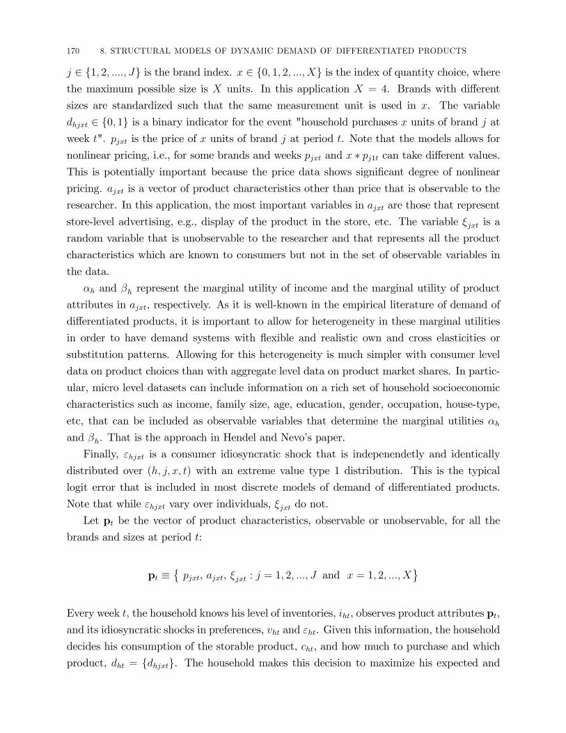
j 2 f1; 2; ::::; Jg is the brand index. x 2 f0; 1; 2; :::; Xg is the index of quantity choice, wherethe maximum possible size is X units. In this application X = 4. Brands with di¤erent

sizes are standardized such that the same measurement unit is used in x. The variable

dhjxt 2 f0; 1g is a binary indicator for the event "household purchases x units of brand j atweek t". pjxt is the price of x units of brand j at period t. Note that the models allows for

nonlinear pricing, i.e., for some brands and weeks pjxt and x � pj1t can take di¤erent values.This is potentially important because the price data shows signi�cant degree of nonlinear

pricing. ajxt is a vector of product characteristics other than price that is observable to the

researcher. In this application, the most important variables in ajxt are those that represent

store-level advertising, e.g., display of the product in the store, etc. The variable �jxt is a

random variable that is unobservable to the researcher and that represents all the product

characteristics which are known to consumers but not in the set of observable variables in

the data.

�h and �h represent the marginal utility of income and the marginal utility of product

attributes in ajxt, respectively. As it is well-known in the empirical literature of demand of

di¤erentiated products, it is important to allow for heterogeneity in these marginal utilities

in order to have demand systems with �exible and realistic own and cross elasticities or

substitution patterns. Allowing for this heterogeneity is much simpler with consumer level

data on product choices than with aggregate level data on product market shares. In partic-

ular, micro level datasets can include information on a rich set of household socioeconomic

characteristics such as income, family size, age, education, gender, occupation, house-type,

etc, that can be included as observable variables that determine the marginal utilities �hand �h. That is the approach in Hendel and Nevo�s paper.

Finally, "hjxt is a consumer idiosyncratic shock that is indepenendetly and identically

distributed over (h; j; x; t) with an extreme value type 1 distribution. This is the typical

logit error that is included in most discrete models of demand of di¤erentiated products.

Note that while "hjxt vary over individuals, �jxt do not.

Let pt be the vector of product characteristics, observable or unobservable, for all the

brands and sizes at period t:

pt ��pjxt, ajxt, �jxt : j = 1; 2; :::; J and x = 1; 2; :::; X

Every week t, the household knows his level of inventories, iht, observes product attributes pt,

and its idiosyncratic shocks in preferences, vht and "ht. Given this information, the household

decides his consumption of the storable product, cht, and how much to purchase and which

product, dht = fdhjxtg. The household makes this decision to maximize his expected and

3. MODEL 171

discounted stream of current and future utilities,

Et (P1

s=0 �s [uh(cht+s; vht+s)� Ch(ih;t+s+1) +mht+s])

where � is the discount factor.

The vector of state variables of this DP problem is fiht, vht, "ht, ptg. The decision vari-ables are cht and dht. To complete the model we need to make some assumptions on the

stochastic processes of the state variables. The idiosyncratic shocks vht and "ht are assumed

iid over time. The vector of product attributes pt follows a Markov processes. Finally,

consumer inventories iht has the obvious transition rule:

ih;t+1 = ih;t+1 � cht +�PJ

j=1

PXx=0 dhjxt x

�where

PJj=1

PXx=0 dhjxt x represents the units of the product purchased by household h at

period t.

Let Vh(sht) be the value function of a household, where sht is the vector of state variables

(iht, vht, "ht, pt). A household decision problem can be represented using the Bellman

equation:

Vh (sht) = maxfcht;dhtg

[uh(cht; vht)� Ch(ih;t+1) +mht + � E (Vh (sht+1) j sht; cht; dht)]

where the expectation E (: j sht; cht; dht) is over the distribution of sht+1 conditional on (sht;cht; dht). The solution of this DP problem implies optimal decision rules for consumption

and purchasing decisions: cht = c�h (sht) and dht = d�h (sht) where c�h (:) and d

�h(:) are the

decision rules. Note that they are household speci�c because there is time-invariant house-

hold heterogeneity in the marginal utility of product attributes (�h and �h), in the utility

of consumption of the storable good uh, and in inventory holding costs, Ch.

The optimal decision rules c�h (:) and d�h(:) depend also on the structural parameters of

the model: the parameters in the utility function, and in the transition probabilities of the

state variables. In principle, we could use the equations cht = c�h (sht) and dht = d�h (sht) and

our data on (some) decision and state variables to estimate the parameters of the model. To

apply this revealed preference approach, there are three main issues we have to deal with.

First, the dimension of the state space of sht is extremely large. In most applications of

demand of di¤erentiated products, there are dozens (or even more than a hundred) products.

Therefore, the vector of product attributes pt contains more than a hundred continuous

state variables. Solving a DP problem with this state space, or even approximating the

solution with enough accuracy using Monte Carlo simulation methods, is computationally

very demanding even with the most sophisticated computer equipment. We will see how

Hendel and Nevo propose and implement a method to reduce the dimension of the state

space. The method is based on some assumptions that we discuss below.


Second, though we have good data on households purchasing histories, information on

households�consumption and inventories of storable goods is very rare. In this application,

consumption and inventories, cht and iht, are unobservable to the researchers. Not observing

inventories is particularly challenging. This is the key state variable in a dynamic demand

model of demand of a storable good. We will discuss below the approach used by Hendel

and Nevo to deal with this issue, and also the approach used by Erdem, Imai, and Keane

(2003).

And third, as usual in the estimation of a model of demand, we should deal with the

endogeneity of prices. Of course, this problem is not speci�c of a dynamic demand model.

However, dealing with this problem may not be independent of the other issues mentioned

above.

3.2. Reducing the dimension of the state space. Given that the state variables(vht, "ht) are independently distributed over time, it is convenient to reduce the dimension of

this DP problem by using a value function that is integrated over these iid random variables.

The integrated value function is de�ned as:

�Vh(iht;pt) �ZVh(sht) dF"("ht) dFv(vht)

where F" and Fv are the CDFs of "ht and vht, respectively. Associated with this integrated

value function there is an integrated Bellman equation. Given the distributional assumptions

on the shocks "ht and vht, the integrated Bellman equation is:

�Vh(iht;pt) = maxcht;dht

Zln

0@ JPj=1

exp

8<: uh(ch; vht)� Ci(iht+1) +mht

+� E��Vh(iht+1;pt+1) j iht;pt; cht; dht

�9=;1A dFv(vht):

This Bellman equation is also a contraction mapping in the value function. The main

computational cost in the computation of the functions �Vh comes from the dimension of the

vector of product attributes pt. We now explore ways to reduce this cost.

First, note that the assumption that there is only one inventory, the aggregate inven-

tory of all the products, and not one inventory for each brand, fihjtg, has already reducedimportantly the dimension of the state space. This assumption not only reduces the state

space but, as we see below, it also allows us to modify the dynamic problem, which can

signi�cantly aid in the estimation of the model.

Taken literally, this assumption implies that there is no di¤erentiation in consumption:

the product is homogenous in use. Note, that through �jxt and "ijxt the model allows

di¤erentiation in purchase, as is standard in the IO literature. It is well known that this

di¤erentiation is needed to explain purchasing behavior. This seemingly creates a tension in

the model: products are di¤erentiated at purchase but not in consumption. Before explaining

3. MODEL 173

how this tension is resolved we note that the tension is not only in the model but potentially

in reality as well. Many products seem to be highly di¤erentiated at the time of purchase but

its hard to imagine that they are di¤erentiated in consumption. For example, households

tend to be extremely loyal to the laundry detergent brand they purchase �a typical household

buys only 2-3 brands of detergent over a very long horizon �yet its hard to imagine that the

usage and consumption are very di¤erent for di¤erent brands.

A possible interpretation of the model that is consistent with product di¤erentiation in

consumption is that the variables �jxt not only captures instantaneous utility at period t but

also the discounted value of consuming the x units of brand j. This is a valid interpretation

if brand-speci�c utility in consumption is additive such that it does not a¤ect the marginal

utility of consumption.

This assumption has some implications that simplify importantly the structure of the

model. It implies that the optimal consumption does not depend on which brand is pur-

chased, only on the size. And relatedly, it implies that the brand choice can be treated as a

static decision problem.

We can distinguish two components in the choice dht: the quantity choice, xht, and the

brand choice jht. Given xht = x, the optimal brand choice is:

jht = arg maxj2f1;2;:::;Jg

��h ajxt � �h pjxt + �jxt + "hjxt

Then, given our assumption about the distribution of "hjxt, the component mht of the utility

function can be written as mht =PX

x=0 !h(x;pt)+eht where !ht(x;pt) is the inclusive value:

!h(x;pt) � E

�max

j2f1;2;:::;Jg


j xht = x; pt

�

= ln

JPj=1

exp��h ajxt � �h pjxt + �jxt

!and eht does not depend on size x (or on inventories and consumption), and therefore we can

ignore this variable for the dynamic decisions on size and consumption.

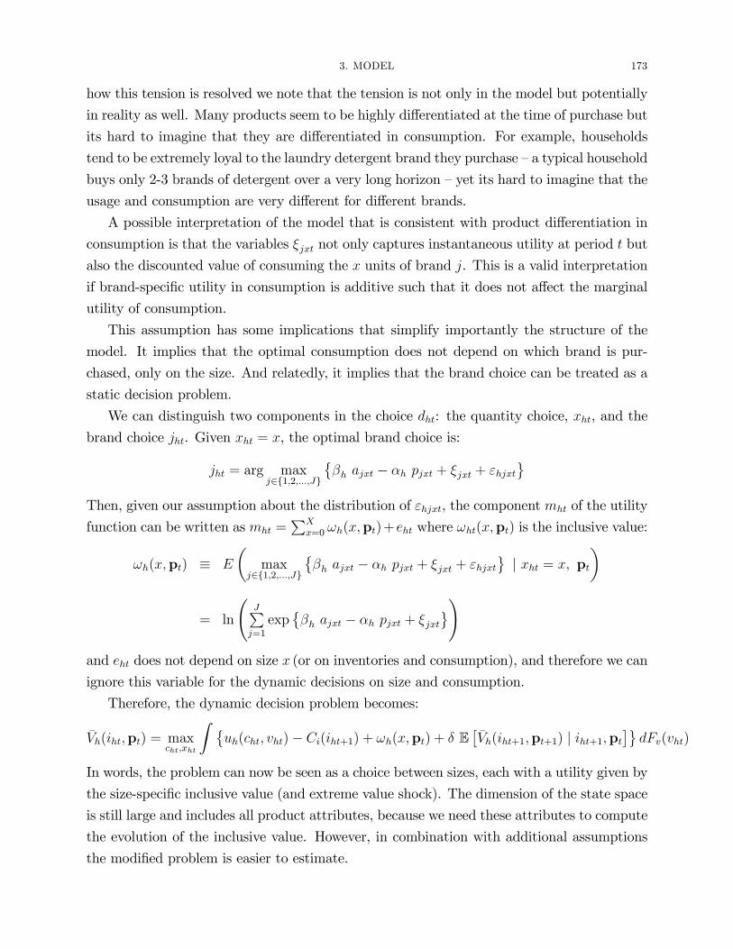
Therefore, the dynamic decision problem becomes:

�Vh(iht;pt) = maxcht;xht

Z �uh(cht; vht)� Ci(iht+1) + !h(x;pt) + � E

��Vh(iht+1;pt+1) j iht+1;pt

�dFv(vht)

In words, the problem can now be seen as a choice between sizes, each with a utility given by

the size-speci�c inclusive value (and extreme value shock). The dimension of the state space

is still large and includes all product attributes, because we need these attributes to compute

the evolution of the inclusive value. However, in combination with additional assumptions

the modi�ed problem is easier to estimate.


Note also, that expression that describes the optimal brand choice, jht = argmaxj2f1;2;:::;Jg{�h ajxt � �h pjxt + �jxt + "hjxtg is a "standard" multinomial logit model with the caveatthat prices are endogenous explanatory variables because they depend on the unobserved

attributes in �jxt. We describe below how to deal with this endogeneity problem. With

household level data, dealing with the endogeneity of prices is much simpler than with

aggregate data on market shares. More speci�cally, we do not need to use Monte Carlo

simulation techniques, or an iterative algorithm to compute the "average utilities" f�jxtg.To reduce the dimension of the state space, Hendel and Nevo (2006) introduce the fol-

lowing assumption. Let !h(pt) be the vector with the inclusive values for every possible size

f!h(x;pt) : x = 1; 2; :::; Xg.

Assumption: The vector !h(pt) is a su¢ cient statistic of the information in pt that

is useful to predict !h(pt+1):

Pr(!h(pt+1) j pt) = Pr(!h(pt+1) j !h(pt))

In words, the vector !h(pt) contains all the relevant information in pt to obtain the

probability distribution of !h(pt+1) conditional on pt. Instead of all the prices and attributes,

we only need a single index for each size. Two vectors of prices that yield the same (vector

of) current inclusive values imply the same distribution of future inclusive values. This

assumption is violated if individual prices have predictive power above and beyond the

predictive power of !h(pt).

The inclusive values can be estimated outside the dynamic demand model. Therefore,

the assumption can be tested and somewhat relaxed by including additional statistics of

prices in the state space. Note, that !h(pt) is consumer speci�c: di¤erent consumers value a

given set of products di¤erently and therefore this assumption does not further restrict the

distribution of heterogeneity.

Given this assumption, the integrated value function is �Vh(iht;!ht) that includes only

X + 1 variables, instead of 3 � J �X + 1 state variables.

4. Estimation

4.1. Estimation of brand choice. Let jht represent the brand choice of household hat period t. Under the assumption that there is product di¤erentiation in purchasing but

not in consumption or in the cost of inventory holding, a household brand choice is a static

decision problem. Given xht = x, with x > 0, the optimal brand choice is:

jht = arg maxj2f1;2;:::;Jg


The estimation of demand models of di¤erentiated products, either static or dynamic, should

deal with two important issues. First, the endogeneity of prices. The model implies that

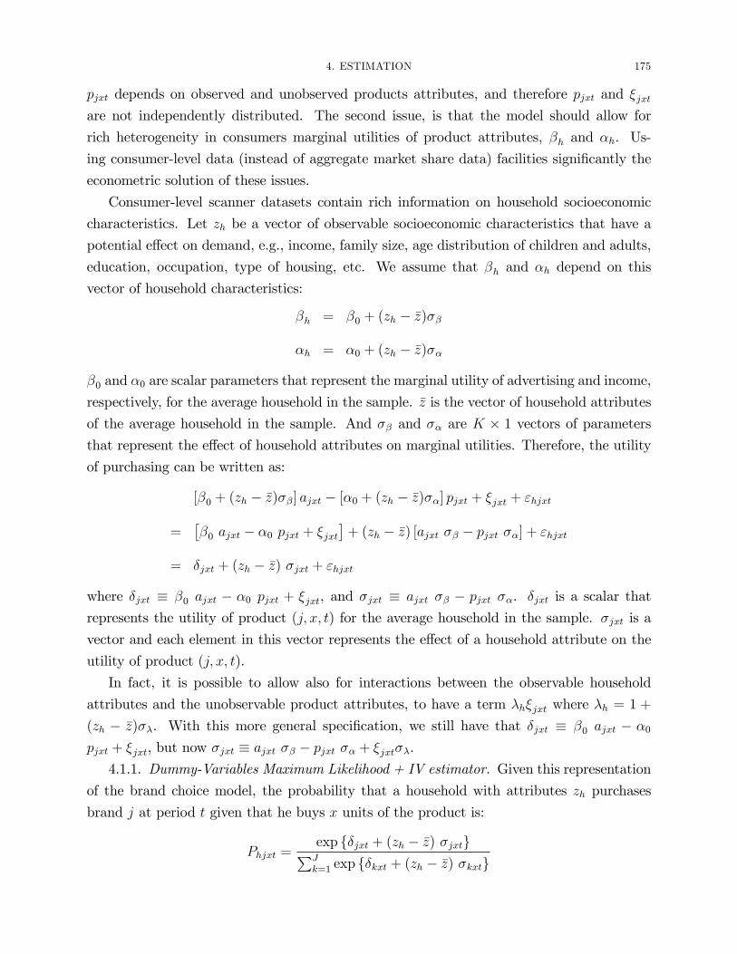
4. ESTIMATION 175

pjxt depends on observed and unobserved products attributes, and therefore pjxt and �jxtare not independently distributed. The second issue, is that the model should allow for

rich heterogeneity in consumers marginal utilities of product attributes, �h and �h. Us-

ing consumer-level data (instead of aggregate market share data) facilities signi�cantly the

econometric solution of these issues.

Consumer-level scanner datasets contain rich information on household socioeconomic

characteristics. Let zh be a vector of observable socioeconomic characteristics that have a

potential e¤ect on demand, e.g., income, family size, age distribution of children and adults,

education, occupation, type of housing, etc. We assume that �h and �h depend on this

vector of household characteristics:

�h = �0 + (zh � �z)��

�h = �0 + (zh � �z)��

�0 and �0 are scalar parameters that represent the marginal utility of advertising and income,

respectively, for the average household in the sample. �z is the vector of household attributes

of the average household in the sample. And �� and �� are K � 1 vectors of parametersthat represent the e¤ect of household attributes on marginal utilities. Therefore, the utility

of purchasing can be written as:

[�0 + (zh � �z)��] ajxt � [�0 + (zh � �z)��] pjxt + �jxt + "hjxt

=��0 ajxt � �0 pjxt + �jxt

�+ (zh � �z) [ajxt �� pjxt ��] + "hjxt

= �jxt + (zh � �z) �jxt + "hjxt

where �jxt � �0 ajxt � �0 pjxt + �jxt, and �jxt � ajxt �� pjxt ��. �jxt is a scalar thatrepresents the utility of product (j; x; t) for the average household in the sample. �jxt is a

vector and each element in this vector represents the e¤ect of a household attribute on the

utility of product (j; x; t).

In fact, it is possible to allow also for interactions between the observable household

attributes and the unobservable product attributes, to have a term �h�jxt where �h = 1 +

(zh � �z)��. With this more general speci�cation, we still have that �jxt � �0 ajxt � �0pjxt + �jxt, but now �jxt � ajxt �� pjxt �� + �jxt��.4.1.1. Dummy-Variables Maximum Likelihood + IV estimator. Given this representation

of the brand choice model, the probability that a household with attributes zh purchases

brand j at period t given that he buys x units of the product is:

Phjxt =exp f�jxt + (zh � �z) �jxtgPJk=1 exp f�kxt + (zh � �z) �kxtg


Given a sample with a large number of households, we can estimate �jxt and �jxt for every

(j; x; t) in a multinomial logit model with probabilities fPhjxtg. For instance, we can estimatethese "incidental parameters" �jxt and �jxt separately for every value of (x; t). For (t = 1,x =

1) we select the subsample of households in sample who purchase x = 1 unit of the product

at week t = 1. Using this subsample, we estimate the vector of J(K + 1) parameters

f�j11; �j11 : j = 1; 2; :::; Jg by maximizing the multinomial log-likelihood function:HXh=1

1fxh1 = 1gJXj=1

1fjh1 = jg lnPhj11

We can proceed in the same way to estimate all the parameters f�jxt; �jxtg.This estimator is consistent as H goes to in�nity for �xed T , X; and J . For a given

(�nite) sample, there are some requirements on the number of observations in order to be

able to estimate the incidental parameters. For every value of (x; t), the number of incidental

parameters to estimate is J(K + 1), and the number of observations is equal to the number

of households who purchase x units at week t, i.e., H(x; t) =PH

h=1 1fxht = xg. We need thatH(x; t) > J(K + 1). For instance, with J = 25 products and K = 4 household attributes,

we need H(x; t) > 125 for every week t and every size x. We may need a very large number

of households H in the sample in order to satisfy these conditions. An assumption that

may eliminate this problem is that the utility from brand choice is proportional to quantity:

x(�h ajt � �h pjt + �jt + "hjt). Under this assumption, we have that for every week t, thenumber of incidental parameters to estimate is J(K + 1), but the number of observations

is now equal to the number of households who purchase any quantity x > 0 at week t, i.e.,

H(t) =PH

h=1 1fxht > 0g. We need that H(t) > J(K+1) which is a much weaker condition.Given estimates of the incidental parameters, f�̂jxt; �̂jxtg, now we can estimate the struc-

tural parameters �0, �0, ��, and �� using an IV (or GMM) method. For the estimation of

�0 and �0, we have that:

�̂jxt = �0 ajxt � �0 pjxt + �jxt + ejxt

where ejxt represents the estimation error (�̂jxt � �jxt). This is a linear regression wherethe regressor pjxt is endogenous. We can estimate this equation by IV using the so-called

"BLP instruments", i.e., the characteristics other than price of products other than j, fakxt :k 6= jg. Of course, there are other approaches to deal with the endogeneity of prices inthis equation. For instance, we could consider the following Error-Component structure in

the endogenous part of the error term: �jxt = �(1)jx + �

(2)jxt where �

(2)jxt is assumed not serially

correlated. Then, we can control for �(1)jx using product-size dummies, and use lagged values

of prices and other product attributes to deal with the endogeneity of prices that comes from

the correlation with the transitory shock �(2)jxt.

4. ESTIMATION 177

For the estimation of ��, and ��, we have the system of equations:

�̂jxt = ajxt�� pjxt �� + �jxt�� + ejxt

where ejxt represents the estimation error (�̂jxt � �jxt). We have one equation for eachhousehold attribute. We can estimate each of these equations using the same IV procedure

as for the estimation of �0 and �0.

Once we have estimated (�0, �0, ��, ��), we can also obtain estimates of �jxt as residuals

from the estimated equation. We can get also consistent estimates of the marginal utilities

�h and �h as:�̂h = �̂0 + (zh � �z)�̂�

�̂h = �̂0 + (zh � �z)�̂�Finally, we can get estimates of the inclusive values:

!̂hxt = ln

JPj=1

expn�̂h ajxt � �̂h pjxt + �̂jxt

o!4.1.2. Control function approach. The previous approach, though simple, has the limita-

tion that we need to have, for every week in the sample, a large enough number of households

making positive purchases. That requirement is not needed for identi�cation of the para-

meters. It is only needed for the implementation of the simple two-step dummy variables

approach to deal with the endogeneity of prices.

When our sample does not satisfy that requirement, there is other simple method that

we can use. This method is a control function approach that is in the spirit of the meth-

ods proposed by Rivers and Vuong (Journal of Econometrics, 1988), Blundell and Powell

(REStud, 2004), and in the speci�c context of demand of di¤erentiated products, Petrin and

Train (Journal of Marketing Research, 2010).

If �rms choose prices to maximize pro�ts, we expect that prices depend on the own prod-

uct characteristics and also on the characteristics of competing products: pjxt = fjxt(at; �t),

where at = fajxt :for any j; xg, and �t = f�jxt :for any j; xg. De�ne the conditional meanfunction:

gpjx(at) � E(pjxt j at) = E(fjxt(at; �t) j at)

Then, we can write the regression equation:

pjxt = gpjx(at) + ejxt

where the error term ejxt is by construction mean independent of at.

The �rst step of the control function method consists in the estimation of the conditional

mean functions gpjx(:) for every brand and size (j; x). Though we have a relatively large

number of weeks in our dataset (more than 100 weeks in most scanner datasets), the number


of variables in the vector at is J �X, that is a pretty large number. Therefore, we need toimpose some restrictions on how the exogenous product characteristics in at a¤ect prices.

For instance, we may assume that,

gpjx(at) = gpjx

�ajxt; �aj(�x)t; �a(�j)xt; �a(�jx)t

�where �aj(�x)t is the sample mean of variable a at period t for all the products of brand j but

with di¤erent size than x; �a(�j)xt is the sample mean for all the products with size x but with

brand di¤erent than j; and �a(�jx)t is the sample mean for all the products with size di¤erent

than x and brand di¤erent than j. Of course, we can consider more �exible speci�cations

but still with a number of regressors much smaller than J �X.The second step of the method is based on a decomposition of the error term �jxt in two

components: an endogenous that is a deterministic function of the error terms in the �rst

step, et � fejxt : for any j and xg, and an "exogenous" component that is independent ofthe price pjxt once we have controlled for ejxt. De�ne the conditional mean function:

g�jx(et) � E(�jxt j et)

Then, we can write �jxt as the sum of two components, �jxt = g�jx(et)+vjxt. By construction,

the error term vjxt is mean independent of et. But then, vjxt is mean independent of all the

product prices because prices depend only on the exogenous product characteristics at (that

by assumption are independent of �jxt) and on the "residuals" et (that by construction are

mean independent of vjxt). Then, we can write the utility of product (j; x) as:

�h ajxt � �h pjxt + g�jx(et) + (vjxt + "hjxt)

The term g�jx(et) is the control function.

Under the assumption that (vjxt+ "hjxt) is iid extreme value type 1 distributed, we have

that the brand choice probabilities conditional on xht = x are:

Phjxt =exp

n�0ajxt � �0pjxt + ajxt(zh � �z)�� pjxt(zh � �z)�� + g

�jx(et)

oPJ

k=1 expn�0akxt � �0pkxt + akxt(zh � �z)�� pkxt(zh � �z)�� + g

�kx(et)

owhere the control functions fg�jx(et)g consists of a brand dummies and polynomial in theresidual variables fejxt : j = 1; 2; :::; Jg. Then, we can estimate (�0, �0, ��, ��) and theparameters of the control function by using Maximum Likelihood in this multinomial logit

model. The log-likelihood function is:

`(�) =

HXh=1

TXt=1

XXx=1

JXj=1

1fxht = x ; jht = jg lnPhjxt

As in the previous method, once we have estimated these parameters, we can construct

consistent estimates of the inclusive values !hxt.

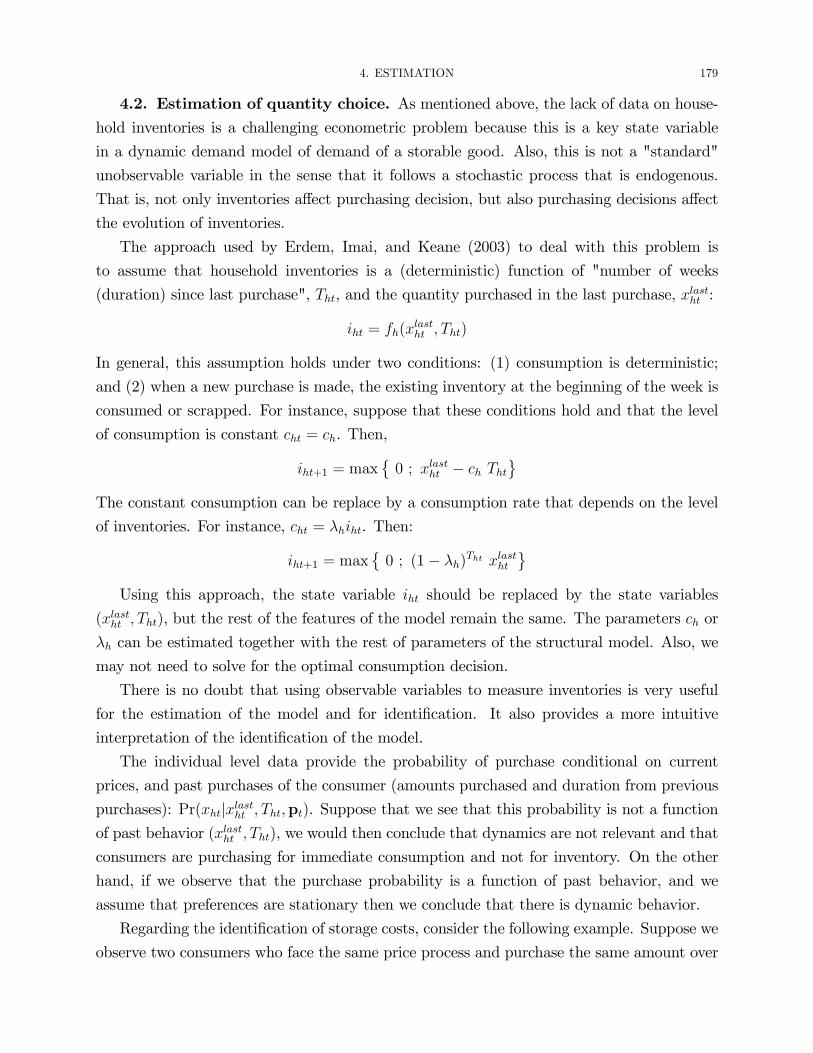
4. ESTIMATION 179

4.2. Estimation of quantity choice. As mentioned above, the lack of data on house-hold inventories is a challenging econometric problem because this is a key state variable

in a dynamic demand model of demand of a storable good. Also, this is not a "standard"

unobservable variable in the sense that it follows a stochastic process that is endogenous.

That is, not only inventories a¤ect purchasing decision, but also purchasing decisions a¤ect

the evolution of inventories.

The approach used by Erdem, Imai, and Keane (2003) to deal with this problem is

to assume that household inventories is a (deterministic) function of "number of weeks

(duration) since last purchase", Tht, and the quantity purchased in the last purchase, xlastht :

iht = fh(xlastht ; Tht)

In general, this assumption holds under two conditions: (1) consumption is deterministic;

and (2) when a new purchase is made, the existing inventory at the beginning of the week is

consumed or scrapped. For instance, suppose that these conditions hold and that the level

of consumption is constant cht = ch. Then,

iht+1 = max�0 ; xlastht � ch Tht

The constant consumption can be replace by a consumption rate that depends on the level

of inventories. For instance, cht = �hiht. Then:

iht+1 = max�0 ; (1� �h)Tht xlastht

Using this approach, the state variable iht should be replaced by the state variables

(xlastht ; Tht), but the rest of the features of the model remain the same. The parameters ch or

�h can be estimated together with the rest of parameters of the structural model. Also, we

may not need to solve for the optimal consumption decision.

There is no doubt that using observable variables to measure inventories is very useful

for the estimation of the model and for identi�cation. It also provides a more intuitive

interpretation of the identi�cation of the model.

The individual level data provide the probability of purchase conditional on current

prices, and past purchases of the consumer (amounts purchased and duration from previous

purchases): Pr(xhtjxlastht ; Tht;pt). Suppose that we see that this probability is not a function

of past behavior (xlastht ; Tht), we would then conclude that dynamics are not relevant and that

consumers are purchasing for immediate consumption and not for inventory. On the other

hand, if we observe that the purchase probability is a function of past behavior, and we

assume that preferences are stationary then we conclude that there is dynamic behavior.

Regarding the identi�cation of storage costs, consider the following example. Suppose we

observe two consumers who face the same price process and purchase the same amount over


a relatively long period. However, one of them purchases more frequently than the other.

This variation leads us to conclude that this consumer has higher storage costs. Therefore,

the storage costs are identi�ed from the average duration between purchases.

Hendel and Nevo use a di¤erent approach, though the identi�cation of their model is

based on the same intuition.

4.2.1. Maximum Likelihood estimation (with proxies for inventories). To Be Completed

4.2.2. Hotz-Miller estimation (with proxies for inventories. To Be Completed

4.2.3. Maximum Likelihood estimation (without proxies for inventories). To Be Com-

pleted

5. Empirical Results

To Be Completed

6. Dynamic Demand of Di¤erentiated Durable Products

- Gowrisankaran and Rysman (2009)

TBW

dynamic structural models of industrial...

Documents