identification of structural dynamic characteristics
TRANSCRIPT
IMPERIAL COLLEGE OF SCIENCE AND TECHNOLOGY
(University of London)
IDENTIFICATION OF STRUCTURAL
DYNAMIC CHARACTERISTICS
bYJimin He
A thesis submitted to the University of London for the degree of
Doctor of Philosophy, and for the Diploma of Imperial College.
Department of Mechanical Engineering
Imperial College, LONDON SW7
October 1987

1__ __
ABSTRACT
Modal analysis is a rapidly growing field in vibration research. It has been used
effectively in the identification of structural dynamic characteristics and has become a
flourishing area of vibration research. There are some aspects of the modal analysis
method which hinder the application of the method to practical cases. Among them are
analytical model correction, damping properties investigation and nonlinearity study. This
thesis seeks to present the newest development on these aspects.
The dynamic characteristics of a vibrating structure are usually predicted by analytical
techniques such as the Finite Element (FE) method. It is believed that errors in the
analytical model are inevitable, while the modal data extracted from measurement are
usually accepted to be correct, albeit incomplete. Hence, the correlation of an FE model
and corresponding measured data becomes a very important process for structural
vibration research. In this thesis, a new technique is developed to locate the area(s) in an
analytical model where the errors are concentrated by using the incomplete modal data
obtained from tests. An iteration process is introduced for the correction of the analytical
model after the errors are localized and the feasibility of these new techniques is assessed
by both theoretical and practical cases.
Associated with the correction of analytical models, this thesis also investigates the
damping properties of a vibrating structure. It is believed that the most significant
damping often comes from the joints between the various components of a structure and a
method is proposed to locate the spatial damping elements from measurements on the
structure. It is also shown that the located damping could then be quantified using the
iteration process.
Nonlinearity is encountered in many practical structures. However, currently available
means for studying this effect are not fully developed. This thesis describes an
advantageous method, based upon a new understanding of the FRF data measured on a
nonlinear system, to identify more conclusively the nonlinearity and to offer much better f
chance for its quantification. This method has been shown to be effective and convenient
in application and could be very useful for further investigation such as modelling the
nonlinearity and/or predicting the vibration response of the nonlinear system.
. /

2-- __
ACKNOWLEDGEMENT
The author is most grateful to his supervisor Professor D J Ewins for his
continuous help and guidance throughout the duration of this research,
and for his sustained advice in the preparation of the manuscript.
Very special thanks are due to Mr D Robb in the Modal Testing Unit who
was most helpful to the author in computing and conducting experiments.
Thanks are also due to Dr P Cawley, Dr C F Beards and Dr M lmregun in
the Dynamics Section for their useful discussions and help.
Finally, the author is indebted to the Government of the People’s Republic
of China for providing the financial support.
L

3-- em
NOMENCLATURE
a
A
Cr
d
i
kij
m
n
N
X
?k
[Cl
[AK,1
WI
[II
RI
wa]R
V&l
W
i”a]R
Wil
subscript for analytical model
modal constant
modal constant of the rth mode
Euclidian norm
imaginary unit
the ‘ij’ element in stiffness matrix
number of measured vibration modes
number of coordinates employed the experimental model
number of coordinates employed by the analytical model
subscript for experimental model
response amplitude of a nonlinear system
symmetric viscous damping matrix (real)
stiffness error matrix, defined as ([KC] - [K,]) (complex)
symmetric structural damping matrix (real)
unity matrix
symmetric analytical stiffness matrix (real)
Guyan-reduced symmetric analytical stiffness matrix (real)
symmetric experimental mass matrix (real)
symmetric experimental stiffness matrix, defined as (&]+i[ITj) (complex)
symmetric analytical mass matrix (real)
Guyan-reduced symmetric analytical mass matrix (real)
symmetric experimental mass matrix (real)

4__ __
AA error on modal constant estimate A
Ml
I(t)
%f@)
s&N
H [WI
F VW1
sgw
k(8
c(%
[ IT
c I-’W 1
In-41
stiffness error matrix, defined as (&,I - [Ka]) (real)
mass error matrix, defined as ([M,] - Ma]) (real)
frequency response function of a dynamic system
impulse response of a dynamic system
cross power spectrum
auto power spectrum
the Hilbert transform of f(x)
the Fourier transform of f(x)
sign function (is equal to one when t is positive and zero when negative)
harmonic response amplitude-dependent stiffness
harmonic response amplitude-dependent viscous damping
transpose of matrix [ ]
inverse of matrix [ ]
the real part of
the imaginary part of
a
a
receptance FRF data
receptance FRF data when the complexity is removed
l/a reciprocal of receptance data
the rth analytical radial natural frequency.
the rth experimental radial natural frequency
radial natural frequency
harmonic response amplitude-dependent natural frequency
the natural frequency of the pfh mode of the updated model after ‘r’
iterations

5__ __
T
s,5(x>
diagonal analytical natural frequency matrix (real)
diagonal experimental natural frequency matrix (real)
analytical mode shape matrix (real)
experimental mode shape matrix (complex or real)
the rth analytical mode shape (real)
the r* experimental mode shape (complex or real)
the ‘pq’ element in the mode shape matrix of the updated model after ‘r’
iterations
damping coefficient of the rth mode
damping loss factor of the rth mode
harmonic response amplitudedependent damping loss factor
c
.-‘I%. . . . _;,.. _.
6__ __
- CONTENTS -
Page
ABSTRACT
ACKNOWLEDGEMENT
NOMENCLATURE
CHAPTER 1 INTRODUCTION
l-l The Identification of Structural Dynamic Characteristics
l-2 Theoretical Prediction Approach
l-3 Experimental Measurement Approach
l-4 Correlation of FE Model and Modal Testing Results
l-5 Nonlinearity
l-6 Preview of Thesis
CHAPTER 2 ANALYTICAL MODEL IMPROVEMENT - THEORETICAL BASIS
2-l Preliminaries
2-2 Some Current Approaches for Model Improvement
2-2-l Matrix Perturbation Theory for Model Improvement
2-2-2 Constraint Minimization Method (CMM)
2-3 The Error Matrix Method (EMM)
2-3-l Principle and Essence of the Error Matrix Method
2-3-2 Validation of the Assumption Made by the EMM
2-4 Model Improvement Using Iteration
2-4- 1 Strategy of the Iteration Process
2-4-2 Criteria for the Assessment of the Iteration Results
2-5 Numerical Study
12
13
14
17
19
20
23
26
26
28
31
31
34 ’
37
38
39
40
. ,

7__ __
2-6 Conclusions 44
CHAPTER 3 LOCATION OF MSMODELLED REGION - NEW DEVELOPMENTS
3-l Preliminaries 61
3-2 Strucmd Connectivity in an Analytical Model 62
3-3 Location of Mismodelled Regions in the Analytical Model 64
3-3-l The Analytical Stiffness Case 64
3-3-2 The Analytical Mass Case 67
3-3-3 General Case 69
3-4 Direct Numerical Calculation of [AK] 70
3-5 Numerical Assessment of Location Technique and Refined Iteration Process 72
3-6 Conclusions 74
CHAPTER 4 IDENTIFICATION OF DAMPING PROPERTIES OF VIBRATING
STRUCTURES
4-l Preliminaries
4-2 Current Approaches for Studying Damping Properties
4-3 Identification of Damping Type from Measured Data
4-3- 1 Methodology for Identification of Damping Types
4-3-2 Removal of Complexity from Measured Data
4-4 Location of Damping Elements from a Structure
4-4- 1 Usual Damping Condition of a Vibrating Structure
4-4-2 The Approach for Damping Element Location
4-5 Estimation of Damping Matrix
4-5-l Extension of the EMM to Estimate Damping Matrix
4-5-2 Iterative Approach to Improve the Estimation of N
4-6 Numerical Assessment of Damping property Investigation
4-7 Conclusions
86
87
90
90
91
92
92
93
95
95
99 +
100
103

8__ __
CHAPTER 5 COMPATIBILJTY OF MEASURED MODES AND ANALYTICAL
MODEL
5-l Preliminaries 117
5-2 Model Condensation by Guyan Reduction 118
5-3 Expansion of Measured Modes by Analytical Model 119
5-4 Comments of Different Approaches 121
5-4 1 Guyan Reduction 121
5-4-2 Expansion of Measured Modes 123
5-5 Expansion of Measured Complex Modes 124
5-6 Assessment of Approaches for Compatibility 126
5-7 Conclusions 127
CHAPTER 6 APPLICATION OF MODELLING ERROR LOCATION TO A
PRACTICAL STRUCTURE
6- 1 Introduction
6-2 Analytical Modelling of the Structure
6-3 Modal Testing of the Structure and Comparison of the Modal Model and
the FE Model
6-4 Location of the Mismodelled Region in the Analytical Stiffness Matrix
Using Measured Vibration Modes
6-4- 1 Expansion of the Measured Vibration Modes
6-4-2 Location of Mismodelled Region in the Analytical Stiffness Matrix
6-5 Conclusions
136
137
138
140
140
140
141
CHAPTER 7 MEASUREMENT OF NONLINEARITY
7- 1 Introduction
7-2 Excitation Techniques
7-2- 1 Sinusoidal Excitation
7-2-2 Random Excitation
c
153
155
155
157
I. . .
9__ __
7-2-3 Transient Excitation
7-2-4 Comments on Different Excitation Techniques
7-3 Practical Considerations of Nonlinearity Measurements
7-4 Simulation for Nonlinearity Investigation
7-4- 1 Significance of Simulation of Nonlinearity
7-4-2 Analogue Simulation of Nonlinearity
7-5 The Frequency Responses of the Nonlinear Systems
7-6 Conclusions
CHAPTER 8 MODAL ANALYSIS OF NONLINEAR SYSTEMS
8- 1 Current Methods and Applications of Modal Analysis
for Nonlinear Systems
8-l-l Bode Plots
8- l-2 Reciprocal of Frequency Response Function
8-l-3 Modal Analysis and the Isometric Damping Plot
8-l-4 The Hilbert Transform
8-l-4- 1 The Principle of the Hilbert Transform
8-l-4-2 Basis of its Application to Modal Analysis
8-2 Comments on Current Methods for the Modal Analysis of Nonlinearity
8-3 A New Interpretation of the Effect of Nonlinearity on FRF Data
8-3-l Interpretation of FRF Data with Nonlinearity
8-3-2 Interpretation of the Reciprocal of Receptance Data with Nonlinearity
8-3-2-l Stiffness Nonlinearity
8-3-2-2 Damping Nonlinearity
8-4 A New Method for the Modal Analysis of Nonlinear Systems
8-4-l Modal Analysis of Stiffness Nonlinearity
8-4-l-l Description of Methodology
8-4-l-2 Algorithm for Modal Analysis of Nonlinear Stiffness
8-4-2 Modal Analysis of Damping Nonlinearity
8-4-3 The Extraction of an Accurate Modal Constant Estimate
158
160
161
163
163
164
168
171
187
188
189
191
192
193
194
197
198
198
201
201
203
204
204 0
205
206 ’
208
209

__ I()__
8-5 Application of the New Method for the Modal Analysis of Nonlinearity 211
8-5- 1 Analysis of Stiffness Nonlinearity 212
8-5-2 Analysis of Damping Nonlinearity 213
8-5-3 Practical Applications of the New Method 213
8-6 Conclusions 215
CHAPTER 9 CONCLUSIONS AND SUGGESTION FOR FURTHER STUDIES
9- 1 Analytical Model Improvement Using Modal Testing Results 239
9-2 Damping properties of Practical Structures 241
9-3 Compatibility of Analytical Model and Measured Vibration Modes 242
9-4 Nonlinearity in Modal Testing 243
9-5 Suggestion for Further Studies 244
APPENDICES
APPENDIX 1: Matrix Perturbation Results 247
APPENDIX 2: Inverse of a Complex Matrix 250
APPENDIX 3: FE Analysis of a Beam Element 252
REFERENCES 254
..,*r, .._, . ..,

c

-- 12 __
CHAPTER1
INTRODUCTION
l-l THE IDENTIFICATION OF STRUCI’URAL DYNAMIC CHARACT’EmCS
In many practical circumstances, the vibration characteristics of a dynamic structure
require to be understood and, subsequently, an accurate mathematical model needs to be
derived. Such a model is needed for response and load prediction, stability analysis,
system design, structural coupling etc.
Since a dynamic structure is a continuous system rather than a discrete one, theoretically,
an infinite number of coordinates are necessary to specify the position of every point on
the structure and hence the structure can be said to have an infinite number of degrees of
freedom. Its vibration characteristics should then include an infinite number of vibration
modes and cover the active frequency range from zero to infinity. However, for most
practical applications, only a certain frequency range is of major interest and only those
vibration characteristics which fall in this range will be investigated. In this case, only a
certain number of vibration modes are to be sought and it becomes feasible to represent
the continuous system by an approximate, discrete, one.
For a discrete linear dynamic system with lumped masses and massless elastic
components, theory has been well developed to study such vibration characteristics. This
is because the differential equations of a discrete linear dynamic system are generally
available, and hence mathematics can be introduced directly to solve the equations of
motion and the vibration characteristics can then be defined accurately. For a truly
continuous system, such as a practical structure, such advantages do not exist. However,
like many other sciences to achieve good approximation by discretization, the strategy of
investigating the vibration characteristics of a practical structure relies basically on the
.
.

__ 13 __
hypothesis of discretizing the structure so that the theory for discrete systems can then
apply and the mathematical model for the structure can then be built. It is evident that as
the number of coordinates employed in the discretization approaches infinity, the discrete
system will approach the continuous one.
Basically, there are two ways of achieving a mathematical model for a dynamic structure
with the help of the discretization concept, they being by theoretical prediction and by
experimental measurement respectively. Both approaches effectively assume that the
vibration characteristics of a continuous system within certain frequency range can be
described approximately by a limited number of coordinates. In the following, both
approaches are reviewed briefly.
1-2 TIIEORE-I’ICAL PREDICI-ION APPROACH
Physics and mathematics have been so developed nowadays that for commonly
encountered mechanical components, such as beams and plates, accurate analytical
solutions are readily available to predict their vibration characteristics. For instance, the
natural frequencies and mode shapes of a lengthy uniform beam could now be easily
computed.
For a rather complicated practical structure, however, there is generally no analytical
solution to predict its vibration characteristics. With the help of new computational
technology, the Finite Element (FE) approach is now widely used in the study of the
vibration characteristics of various practical structures. The fundamental principle of the
FE method is to discretize a complicated structure into many small elements. For each
such an element, known as a finite element, the mass and stiffness properties are assumed
to obey a known and relatively simple linear pattern. Thus, the mass and stiffness
matrices of an element can be constructed. The global mass and stiffness matrices of the
structure can be assembled using these element matrices and also by considering the
connectivity and the boundary conditions. These global mass and stiffness matrices,
c

-- 14 __
which actually constitute the so-called FE (analytical) model for the structure, can then be
used to derive the description of the vibration characteristics of the structure, namely, the
natural frequencies and mode shapes.
The natural frequencies and mode shapes derived from the global mass and stiffness
matrices from the FE model are often referred to as undamped natural frequencies and
undamped mode shapes since the damping properties for a structure cannot be predicted
in the same way as mass and stiffness and a FE model does not normally include a
damping matrix. Although an approximation for the damping properties can be made by
introducing a proportional damping matrix (i.e. to assume that damping matrix is
proportional to a linear combination of the mass and stiffness matrices), the mode shapes
obtained from such a FE model are still the same as the undamped ones. Besides, it has
been generally accepted that damping properties thus predicted can be incorrect in most
cases.
1-3 EXPERIMENTAL MEASUREMENT APPROACH
Apart from the approach of theoretical prediction to achieve a analytical model for the
study of vibration characteristics of a dynamic system, another major approach is to
establish an experimental model for the system by performing vibration tests and
subsequent analysis on the measured data. This process, including the data acquisition
and the subsequent analysis, is now known as ‘Modal Testing’. In the last two decades,
modal testing (it is believed that this name is much younger than its real practice)
continues to develop, both in theory - new methodology, and in practice - new test
techniques and modern instrumentations - because of continuous new challenges fromc
real life and capabilities offered by powerful computer technology. It is not surprising that
modal testing has penetrated into many branches of engineering.
In common with the approach of theoretical prediction, modal testing assumes that the
vibration characteristics of any systems or structures, discrete or continuous, can be

__ 15 __
described by a selected number of coordinates within a frequency range of interest. In
reality, modal testing can serve many purposes according to different requirements. In
vibration engineering, current modal testing practice has shown its application in various
aspects and they can be categorized briefly as follows:
(i) The most significant application of modal testing is perhaps to produce modal data
(natural frequencies, damping loss factors and mode shapes) of a dynamic system so
that they can be used to compare with the corresponding modal data produced by the
system’s analytical model, in order eventually to validate the analytical model itself.
Further investigation involves using the experimental model consisting of the derived
modal data to improve the analytical model - a practice known as model improvement
or correlation of the experimental and analytical results - and this is substantially
studied in this thesis;
(ii) In the absence of an analytical model, the experimental modal data are used sometimes
to construct a spatial mathematical model for a dynamic system which will then be
used to predict the effects of modifications on the system and to conduct sensitivity
analysis.
(iii) For some practical structures consisting of various components, direct testing may
present certain difficulties. If mathematical models can be obtained for each
component, and boundary conditions are correctly assumed, then a global model can
be constructed. This process, often referred to as ‘substructuring’ or ‘modal
synthesis’, requires an accurate derivation of the modal data from modal testing for
each component.c
(iv) In the absence of an analytical model, an experimental model consisting of the modal
data is sometimes used to predict the system’s vibration response under certain
external excitation conditions. Alternatively, it can also be used to determine the
dynamic loading if the vibration responses of the system are measured.

__ 16 __
Modal testing practice involves two major aspects: measurement to acquire data
(frequency response function or time domain response) and modal analysis to extract a
modal, or experimental, model. Although the final goal of modal testing is produced by
the analysis, the importance of measurement could never be overstressed.
Currently, there are two main excitation techniques in common use, they being of single
point excitation and multi-point excitation. The single point excitation method excites a
structure at one coordinate and measures the response at all the coordinates. Theoretically,
such a test - one point excitation and multi-point responses - is sufficient for the
subsequent analysis in order to extract the experimental model. However, it is often found
that the single excitation point is not appropriate to expose all the vibration modes of
interest. Thus, changing the excitation point and repeating the measurement for several
points is essentially required. This single point excitation method involves less
instrumentation, employs inexpensive computer software and is easy to master, but is
obviously not suitable for exciting a large structure. Unlike the single point excitation
method which excites a structure to vibrate in several modes simultaneously, the
multi-point excitation method attempts to excite a structure in order to eliminate the
unwanted modes so as to get a single pure mode. This brings about a significant
advantage for the subsequent analysis. The price, however, is paid to require much more
sophisticated instrumentation and the measurement operation could become very
involved.
The data acquired from measurement are to be analysed in different ways, depending on
the different requirements made of the data. It is believed that the direct requirement in
most cases is to derive the natural frequencies, damping loss factors and mode shapes.
Since the data acquired from measurement are normally in the form of frequency response
functions, two methods are widely applied in the modal analysis process known as
‘Single Degree-of-freedom (SDOF) Curve-Fit’ and ‘Multi-Degree-of-freedom (MDOF)
Curve-Fit’ respectively.
c

__ 17 --
The SDOF curve-fit method assumes that, in the vicinity of a resonance, the frequency
response function is dominated by this vibration mode and can therefore be approximated
to that of a SDOF system plus a constant quantity, which is usually referred to as the
‘residual’. Thus, by applying the nature of the Nyquist circle or its equivalent for a SDOF
system, a curve-fit can be made for each mode to extract the natural frequency, modal
constant and damping loss factor. Although the assumption itself restricts the condition of
close modes, it is found in practice that using an iterative process for this SDOF curve-fit
method even cases with close modes could often produce satisfactory results.
The MDOF curve-fit method seeks to derive a theoretical frequency response function
which provides a “best fit” to the measured frequency response data. Since it operates for
several modes simultaneously, it can be used directly for the case of close modes when
the interactions among vibration modes are taken care of at the same time. Besides, when
the damping in measured data is so small to cause difficulties on Nyquist circle-fit, the
MDOF curve-fit method can still analyse the data[l].
Among other methods being used in the analysis of measured data, Ibrahim Time Domain
method (ITD) is one of the noticeable techniques. Unlike the previous descriptions, the
lTD makes use of the measured data in time domain form (rather than frequency domain).
The basic idea of ITD is to extract the modal data from the free decay response of a
system. Once the free decay response is measured or computed from other forms of data,
the modal data extraction can be made routine, requiring much less interactive effort. This
characteristic accelerates the analysis process, while in the mean-time loses visual control
of the modal data extraction and, as a result, could end up with unrealistic results in some
circumstances.
l-4 CORRELATION OF FE MODEL AND MODAL TESTING RESULTS
Due to their own respective advantages, both the Finite Element approach and Modal
._ I

testing approach are widely used nowadays to study the vibration characteristics of
dynamic systems and structures. The FE method predicts the vibration characteristics by
theoretical studies so that no experimental facilities are needed. It can employ a large
number of coordinates so that the vibration characteristics can be described in detail and
can cover a comparatively wide frequency range. In addition, it can be used at the design
stage to predict the vibration behaviour of a future structure and, possibly, to modify the
blueprint. However, due to the crucial complexity of practical structures, especially the
joints between the components in them, the modelling of the mass and stiffness properties
could be inaccurate or even incorrect, and that of the damping properties is generally
artificial or omitted altogether. Modal testing is supposed to identify the ‘true’ vibration
characteristics of a structure, since it deals with the real object rather than an idealisation.
Thus, the experimental model possesses the information of the ‘correct’ mass, stiffness
and damping properties. However, due to the limited number of coordinates and
incomplete number of modes - both are the consequences of various practical restrictions
in measurement - the information thus obtained is available primarily as the modal
parameters, rather than the spatial properties as provided by the FE model.
No doubt, differences will exist between the FE model and the experimental model.
The principle of correlating the models derived from these two different approaches is
basically to make use of the advantages on both and to overcome their disadvantages.
Since a representative spatial model is increasingly demanded in vibration practice, current
efforts are mainly directed to using modal testing results to improve or to correct the FE
model. This is nowadays often referred to as ‘model improvement’ or ‘model correction’.
In a model improvement study, the advantages of both modal testing results - containing
correct information (albeit incomplete) of the vibration characteristics - and of the FE c
model - a complete model - are retained. The improved model is expected to be a better
approximation of the correct but unavailable model.

__ 19 --
l-5 NONLINEARITY
In the previous description, there is an important assumption for using the two main
approaches to identify vibration characteristics, namely, that the dynamic system to be
studied should behave linearly in vibration. In general, a dynamic system is said to be
linear if: (i) doubling the input force will double the vibration response and (ii) the
summation of the responses due to two independent inputs should be the same of the
response due to the summation of these two inputs. Failure to obey these relationships
implies the structure to be nonlinear. Thus, the measured frequency response function
data of a linear dynamic system from different tests with different force levels should be
the same.
It is believed that all real structures have a certain degree of nonlinearity. In many cases,
they are regarded as linear structures because the degree of nonlinearity is small and
therefore insignificant in the response range of interest. While in other cases, nonlinearity
may have to be tolerated simply because of lack of effective means to cope with it.
Basically, the existence of nonlinearity has two consequences in the realm of identification
of vibration characteristics. Firstly, the analytical model of a nonlinear system will be
erroneous because, unless a real measurement is taken, the existence of nonlinearity
usually cannot be foreseen merely by theoretical prediction and nor can it be quantified
theoretically. Secondly, since the frequency response function data become input
force-dependent, the significance of the modal parameters extracted by modal testing has
to be considered much more carefully.
The theoretical study of known types of nonlinearity such as cubic stiffness can be dated ’
back to the beginning of this century. Although the nonlinearity described by known
differential equations has been thoroughly understood in textbooks, the difficulty faced by
modal testing is to investigate unknown type(s) of nonlinearity from practical structures.
Nevertheless, using modal testing techniques to study the theoretical or simulated data

__ 20 __
with known type(s) of nonlinearity paves the way to an understanding of nonlinearity in
practical structures. Once the types of nonlinearity most commonly encountered in
practice have been categorised by their effects on modal data, the results can be referenced
helpfully by the analysis of measured data from real structures.
Current efforts in modal testing practice are directed towards the detection and
identification of nonlinearity in real structures, although the quantification of nonlinearity
is still in its infancy. The detection of the existence of nonlinearity from measured data is
believed to be relatively much easier, if the excitation method is properly selected and
measurement is performed appropriately. However, it is its identification that has attracted
most efforts in modal testing study. Despite the complexity of practical structures, the
main difficulty for the identification is to be able to produce a conclusive answer from the
analysis.
l-6 PREVIEW OFTHETHESIS
Despite the rapid development in the identification of dynamic characteristics of structures
in recent decades, there are still some aspects in modal analysis research with common
interests, which hinder the vast application of modal analysis to practical cases. Among
these aspects, damping properties of structures, analytical model correction using modal
testing results and nonlinearity are three notable subjects. The research project presented
in this thesis is intended to seek new improvements on these three subjects and, as a
result, to pursue better understanding of the dynamic characteristics of structures.
Conventional methods to modify, or to correct, an FE model using modal testing results
are discussed in Chapter 2, including the perturbation method, the constraint minimization
method and the error matrix method. It is found that, when the number of measured
vibration modes is insufficient, these methods could not successfully improve the FE
model. In fact, the resultant model suggested by these methods could be mathematically
optimal although physically unrealistic, Since it is generally accepted that errors existed in

__ 21 --
an FE model are often small and isolated, efforts in this thesis are directed towards first
enabling to locate the existent errors and then to correct them objectively rather than to
modify the whole model. Chapter 3 presents the development of a new technique to locate
the errors in an FE model using a very limited number of measured modes. It is then
suggested that an FE model should be improved by only correcting the located errors
using the measured modes. In Chapter 4, damping properties are studied in order to offer
an existing FE model with a sensible damping model, rather than merely a proportional
one or none at all.
One of the practical difficulties faced by the model correlation process is the
incompatibility of the FE model and the modal testing results in the sense of the adopted
coordinates. Chapter 5 concentrates on resolving this difficulty. Both undamped and
damped conditions are investigated. The new development in this study is assessed by a
practical application presented in Chapter 6.
For those cases where nonlinearity cannot realistically be ignored, Chapters 7 and 8 seek
to investigate this phenomenon by modal testing techniques. The measurement of
nonlinear systems is discussed in Chapter 7, including the excitation methods and the
simulation of various commonly encountered types of nonlinearity. In Chapter 8, the
present development of nonlinearity study is discussed and summarized. Based upon
these present developments and a new interpretation of the effect of nonlinearity on modal
data, a new method is proposed to identify the nonlinearity from measured data.
Finally, Chapter 9 reviews all the new developments presented in this thesis and exhibits
the direction from which possible further studies can be cultivated.c

c

__ 23 __
CHAPTER 2
ANALYTICAL MODEL IMPROVEMENT -
THEORETICAL BASIS
2-l PRELIMINARIES
When the identification of structural dynamic characteristics is undertaken by both of the
two widely-used techniques, i.e. (1) theoretical analysis (normally by Finite Elements)
and (2) modal testing and analysis, an inconsistency often exists between the vibration
data predicted by the theoretical model and those identified experimentally. Although the
argument of what causes this inconsistency has been raised[4], it is nowadays often
believed, that more confidence can be placed on the experimental modal data than on
either the analytical mass or stiffness matrices and, as a consequence, the analytical model
of a structure should be modified upon the basis of the experimental modal data, provided
this modification is required in practice. In this Chapter, we shall deal mainly with
systems with little damping so that all the vibration modes involved are real. Special
interest is paid to the stiffness properties although it will be seen that the methodology can
be similarly applied to the mass properties. The darnping and complex mode case will be
investigated in Chapter 4.
When both an analytical model of a structure and experimental modal data are available,
the analytical model improvement can be cast into the following mathematical problem:
>>> for a linear and undamped system, the dynamic characteristics (natural
frequencies and mode shapes) can be described by a set of second order
differential equations:
L -

__ 24 __
[M,lI:l + [KJxl = (0) (2-l)
where [M,] and [KJ are NxN approximate (due to modelling errors) mass and
stiffness matrices, comprising the analytical model of the system
The “analytical” modal data (natural frequencies and mode shapes) can be
derived by solving equation (2-l), yielding a set of solutions:
tK,l - (yJ,2[Mal)(4& = WI (2-2)
where (o,)~ and {Q,}, (x=1, . . . N) are the r* mode analytical natural frequency
and mode shape respectively. All the mode shape vectors are Nxl in
dimension.
Meanwhile, the modal data from measurement provide the experimental natural
frequencies (O,.)r and mode shapes (Q,}, (r=l, . . . m), and have all the mode
shape vectors {@Jr are nxl in dimension. They are incomplete (because not all
coordinates are measured) and relate to an experimental model consisting the
experimental mass matrix [MJ and stiffness matrix [K,] which are generally
close to, but different from, their analytical counterparts [MJ and [K,]. The
difference between the analytical mass (or stiffness) matrix and the
experimental mass (or stiffness) matrix can be represented by a mass error
matrix [AM] (or stiffness error matrix [AK]).
c
It is supposed that the analytical model (W,] and [KJ) needs to be updated
using the experimental modal data (6.Q and {+,Jr, (x=1, . . . m) so that it
represents more accurately the dynamic characteristics of the modelled
structure. cc<

__ 25 __
In recent years, a number of methods have been published in the literature to deal with
analytical model improvement by a variety of approaches. It is believed that the problem
of model improvement was fust addressed intuitively by Berman and Flannelly[5]. In the
paper, they stress the incompleteness involved in model improvement and suggest that
measured vibration modes are used to improve an analytical mass matrix and to identify
an ‘incomplete’ stiffness matrix, although the stiffness matrix thus deduced is certainly
not appropriate from today’s point of view. Collins et alC6] employ a technique of
statistical parameter estimation in an iterative procedure to adjust an analytical model.
Instead of directly improving the constructed analytical mass and stiffness matrices, their
technique seeks to modify the physical parameters (such as mass per unit length) of which
the analytical model consists. Although the method preserves the connectivity of the
original analytical model during the iterative procedure, the formulation of the method
restricts its application for practical structures. Matrix perturbation theory was later
~~~uc~[71S31 as an attempt to modify an analytical model using measured modes. On
the other hand, Baruch and Bar Itzhack[9]~[10] employed constraint minimization theory
from control engineering in model improvement and developed formulations to modify
the analytical stiffness and flexibility matrices after the measured vibration modes are
optimized using analytical mass matrix, based upon orthogonality property. The resultant
model thus modified has analytical modes identical to the corresponding measured modes
used. Having considered that analytical mass matrix improvement could be the primary
goal (rather than the stiffness case), Be-L1 11 applied the same constraint minimization
theory and obtained a modified analytical mass matrix using measured modes. Later,
Caesar[12] developed an algorithm to apply these formulations derived from constraint
minimization theory. Some applications of model improvement are also found in the ’
literature[14]~[151. Apart from the methods summarised above, the Error Matrix
Method[161 is notably different from others. It aims at using the measured vibration
modes to locate errors existing in an analytical model.

__ 26 __
In the following, some of the methods which have been mentioned are summarised.
Moreover, the Error Matrix Method (EMM) has been given special attention in this thesis
and will be studied in detail later in this chapter.
22 SOME CLIRRENT APPROACHES F’ORMODEL IMPROVEMENT
2-2-l Matrix Perturbation Theory for Model Improvement
The essential objective of analytical model improvement can be stated as aiming to find the
differences between the analytical model mass and stiffness matrices [MJ and [K,] and
the experimental model mass and stiffness matrices [q] and &I, the former matrices
being assumed erroneous and the latter ones to be correct. Since the difference between
these two models is generally believed to be small compared with the analytical model
itself, it is supposed (here) that [AM] could be regarded as the perturbation of the
analytical mass matrix [M,], which consequently leads w,] to the perturbed mass matrix,
[M,]. The same argument can be made for the stiffness matrix case. Thus, matrix
perturbation theory can be applied to develop a relationship between the perturbations
[AM] and [AK] and the corresponding differences in the modal data, including natural
frequencies and mode shapes.
Supposing the analytical model of a system ([MJ and [K,]) differs from the assumed
correct experimental model ([MJ and [KJ) by [AM] and [AK], then
&I = [MaI + WEI
[&I = &I + WI
(2-3) +
(2-4)
The consequence of introducing [AM] and [AK] on the predicted modal properties can be
__ 27 __
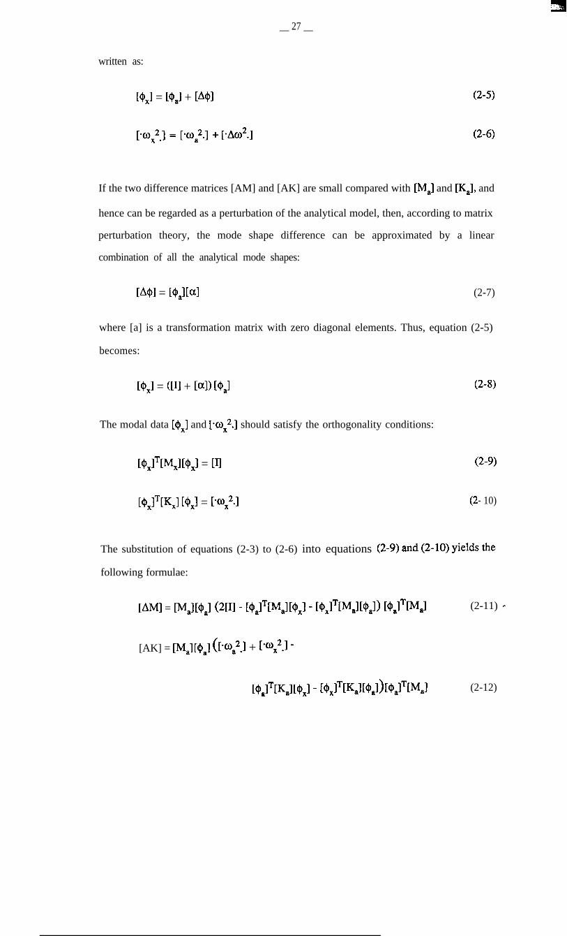
written as:
[@,I = NJ + [Ml
[xox2_] = [x0,2.] + [-Ao2.]
G-5)
(2-6)
If the two difference matrices [AM] and [AK] are small compared with [M,] and [KJ, and
hence can be regarded as a perturbation of the analytical model, then, according to matrix
perturbation theory, the mode shape difference can be approximated by a linear
combination of all the analytical mode shapes:
Ml = [@Jai (2-7)
where [a] is a transformation matrix with zero diagonal elements. Thus, equation (2-5)
becomes:
[@,I = ([II + [aI> P&l (2-W
The modal data [$,I and [*wx2.] should satisfy the orthogonality conditions:
r~,pDq[~xl = Kl (2-9)
r~,lTwJ r4q = [‘@x2.l (2- 10)
The substitution of equations (2-3) to (2-6) into equations (2-9) and (2-10) yields the
following formulae:
[AM-j = [M,l[@J (Wl - [@JTIMal[@xl - [~xlTIMal[~,l) [+JTwal (2-11) *
[AK] = [M,I@B] (b’,z.l + [‘O:.l -
[@JTIKal[~,l - [~,lT[KJ[~,l)[~~T[M3 (2-12)

__ 28 __
Equations (2- 11) and (2- 12) represent the relationship between the perturbation matrices
[AM], [AK] and the modal data of the system before and after the perturbation. These
equations give the correct [AM] and [AI(I provided the complete modal data are available.
However, in practice, the high-frequency modes which happen to dominate the estimation
of [AM] and [AK] in the equations are not obtainable from measurement. This makes
these equations less practical in reality.
2-2-2 Constraint Minimization Method (CMM)
The ideal model of a vibration system including mass and stiffness matrices is a model
such that the modal data derived from it should not only satisfy the eigendynamics
properties (see (i) below), but must also satisfy physical constraints such as symmetry
and orthogonahty of the model. Baruch and Bar Itzhack proposed a methodf9] by which
the analytical stiffness matrix [KJ can be improved using experimental modal data. The
method assumes that the analytical mass matrix [M,] is reliably accurate (and hence that
[AM]=[O]) and applies the following physical constraints which the improved stiffness
matrix [KJ is required to satisfy:
(0
(ii)
[K,l [&J = ~M,l[~,l [‘wx2.1 eigendynamics and
&IT = [&I SYmmetry.
The difference between the analytical stiffness matrix [K,] and the objective stiffness
matrix II(x] is evaluated by the following Euclidian norm, which is a physically sensible
and mathematically convenient function:
d = ll[M,l-“2([K,]-[K~])[Mxl.l/211

__ 29 __
The two physical constraints are incorporated by Lagrange multipliers into a Lagrange
function which is to be minimized to derive the optimal stiffness matrix, K]. The final
stiffness matrix thus optimized is given by:
[ql = [K,] - [K,I[@~I [~,lTWxl - [M,l[@J[+,lTIKal +
Alternatively, it may be said that the difference between the optimized and analytical
stiffness matrices is defined by the CMM as:
[AK] = - ~,l[~,lEO~T~M,l - [~l[~xlbt’xlTIKal +
[MJ[$J [y2.] [$,lTIM,l + WJ [$,I [@xlTIKal [+,I [@,lT[%l c2- ’ 3b)
It can be seen from equation (2-13) that this method does not require the analytical modal
data. Instead, it attempts to improve the stiffness distributions which are the physical
parameters by using the experimental modal data directly. This simplifies the procedure of
analytical model improvement. However, the basic assumption that the analytical mass
matrix is reliable - which this method requires - does not hold in some practical cases and
this limits the applicability of this method to improve the analytical stiffness matrix of
practical structures.
It is found that because of the inevitable incompleteness of experimental modal data, the
optimal stiffness matrix deduced by equation (2-13) will somehow dramatically change
the structural connectivity of the system being modified. In this case, the analytical f
stiffness matrix is improved in such a way that the modified model will surely represent
the incomplete modal data from measurement, but at the expense of the structural
connectivity which is also an essential constraint on the model. Hence, it is desirable that
the structural connectivity be imposed directly into this method as another necessary

__ 30 --
constraint so that the stiffness matrix can be adjusted in a more convincing way.
Unfortunately, this is mathematically difficult to achieve.
Berman has successfully applied a similar methodology to the case of analytical mass
improvement[ll]. He imposed the orthogonality constraint during the correction
procedure and derived an optimal mass matrix by minimizing the following Euclidian
norm:
d = II[M,l-1’2([Mxl-[M,1)[MJ-“211
and this yields an optimized mass matrix:
[MJ = [MaI + [M,lD&lbal-’ ([El-[maI) b,]-‘[f&lTIMal (2-14)
where matrix [ma] is a modal mass matrix defined as:
As has been seen above, that the main drawback for the Matrix Perturbation Method is its
b&l = ~o,lT[qb&l
failure to estimate the dominant parts in matrices [AM] and [AK] due to the usual absence
of high frequency modes from the measured data. On the other hand, the Constraint
Minimization Method requires an accurate analytical mass matrix for analytical stiffness
matrix improvement, and this requirement is not likely to be fulfilled in reality. Besides,
the current methods concentrate on modifying the analytical model while few of them pay
attention to locating the errors which exist in the model. Hence, the model improvement
problem somehow needs a different approach and the Error Matrix Method describedc
below is intended to fill this requirement.

__ 31 --
23THEERRORMATRlXMETHOD(EMM)
2-3-l Principle and Essence of the Error Matrix Method @KM)
The Error Matrix Method (~~~$161 is a different approach to the others in the analytical
model improvement study. The EMM correlates the analytical modal data, which are
generated by the analytical model, with the corresponding modal data from measurement
in an attempt to identify and locate the cause of the differences between the analytical
model and the experimental model. To begin with the stiffness case, the EMM first
supposes that the complete experimental stiffness matrix [Kx] is available as well as the
analytical one [K,] and then defines the difference between the two stiffness matrices as
the “stiffness error matrix”:
[AK1 = [%I - [&I (2-15)
Equation (2-15) can be rearranged and inverted on both sides, leading to:
[%1-l = (EK,l + [AK])-’
= [U$l(III + KJ-‘WI)]-’
= [KJ-1 - [KJ’[AK][KJ-’ + [KJ-‘[AK][K,]-‘[AK][KJ-’ - . . . . .
= f&l-’ - (~IWWal-lP+W) &I-’ (2-16)
When that matrix [AK] is small compared with [K,], the matrix product ([KJ’[AK])’
tends to zero as the exponent 9” becomes large. under these conditions, the flexibility
matrix [KJ’ in equation (2-16) can be approximated by:
.%‘ .:.,. -._

__
rq-’ E [KJ-’ - [KJ-‘[AK][K,]-’
so that WI z &,I UKJ-’ - K,J-‘) WJ
32 --
(2- 17)
(2-18)
Equation (2-18) can be used to estimate the stiffness error matrix [AK] by constructing
each of the two flexibility matrices from the corresponding modal data. A flexibility
matrix can be expressed in terms of modal data as follows:
(2-19)
(2-20)
It is realised that, in practice, modal data from measurements are incomplete in two
aspects; one, the number of modes which can be studied (ma) and two, the number of
coordinates which are measured to describe the mode shapes (ncN). Due to these two
sources of incompleteness, the flexibility matrices in equations (2-19) and (2-20) are
necessarily approximated using:
(2-21)
(2-22)
Therefore, a stiffness error matrix can be estimated using the incomplete experimental
modal data and the corresponding analytical modal data from the following expression:
The error matrix thus deduced can be used to identify and to locate the difference(s)
between the experimental stiffness matrix (which is supposed to be correct) and the

__ 33 __
analytical one (which is believed to contain errors).
A similar procedure can be applied in the case of the mass matrix. The mass error matrix
[AM] is defined as the difference between the experimental mass matrix and the analytical
one:
[AMI = W,l - [MaI (2-24)
Following similar algebra to that used for the stiffness case, the mass error matrix can be
estimated as:
[AMI z [MaI WJ-’ - [$I-‘> [MaI (2-25)
(2-26)
Again, the incomplete experimental modal data and the corresponding analytical modal
data are used in to evaluate the mass error matrix [AM].
The essence of the EMM should be noticed. First of all, it does not presume or require an
accurate analytical mass matrix (&@[M,]) for analytical stiffness matrix improvement.
Physically, this means that the stiffness matrix is not determined with a mass matrix being
its direct reference basis. Instead, a group of measured modes is used as the reference
basis. This point is reasonably acceptable in many practical cases such as the
determination of stiffness matrix of a car body where a significant amount of mass comes
from attached objects. (It should be borne in mind here that although the mass matrix [M,]
is not the direct reference basis, it is an implicit one due to the derivation of [$J and [hJ ,
from [MJ and [I&]). Similarly, the EMM does not presume an accurate analytical
stiffness matrix ([K,]=[K,]) for the analytical mass matrix improvement, with the same
advantage. Lastly, the EMM focuses the analytical stiffness matrix improvement on the
flexibility matrix, where lower frequency modes dominate. This agrees with the fact that,

__ 34 __
in practical measurements, only the lower frequency modes are readily available.
Nevertheless, according to the nature of its approximation, the EMM could be applied
repeatedly, in an iterative process, - a feature which is discussed below.
2-3-2 Validation of the Assumption Made by the EMM
Since the Error Matrix Method (EMM) first appeared as a useful tool for analytical model
improvement[16], a number of applications have been reported in recent
literature[l71,[l81,[191 . However, the assumptions made by the method have not yet
been fully assessed and this task will be addressed below. The fundamental assumption
suggested by the EMM is the supposition that the matrix product ([KJ’[AK])’ in
equation (2-17) goes to zero as “r” becomes large so that the higher terms in equation
(2-17) can be ignored.
matrix product ([K,]-l[AK])r goes to zero as 9”
becomes larger so that terms for r22 can be ignored.
This assumption eventually raises a number of subsequent questions if the course of the
derivation of the EMM is carefully inspected, and this, in turn, raises a query about the
physical meaning behind the mathematical manipulation upon which the EMM is derived.
(1) Is [KJ’ G [KJ - (gl(-l)r([KJ-l[AK])r) [K,] a good approximation of [KJ’?
(2) Is [%I = (&I - 2 (- l)-l([K,]-l[AK])r[K,])-l a good approximation of [Kx]?I=1
(3) Will F] thus approximated preserve the connectivity of the original [K,]?
(4) Will [KJ thus approximated preserve the correct location of stiffness errors?
In order to answer these questions and so to assess the fundamental assumption, it is
appropriate to perform some numerical studies for which the exact stiffness error matrix is
c
L ,
__ 35 --
known so that it can be used in the assessment.
A case study has been carried out. The system used was an 8 degree-of-freedom discrete
system shown in Figure 2-l. The lumped masses are connected by light stiffness
components. In order to define a similar, but slightly different system, it is supposed that
the stiffness component between coordinates 2 and 3 is not correctly represented by the
analytical model: the analytical estimate for this component was 1.5E+6 N/m in
comparison with the correct stiffness 1.95E+6 N/m, which is 30% larger than the
analytical stiffness quantity. Apart from this difference, the analytical model coincides
with the experimental model both in stiffness and in mass conditions. Table 2-l contains
the simulated experimental (or correct) stiffness matrix and the analytical (or approximate)
stiffness matrix while the correct [AK] for this case is shown in Figure 2-2. It is to be
demonstrated by this numerical study that the questions put forward above can be
answered positively and, in turn, the assumption employed by the EMM is validated.
It can be seen by re-examining equation (2-16) that the matrix product ([KJ“[AK])’
(r=1,2, . . . ) is virtually a weighting factor for matrix [Ka] in each term on the right hand
side of the equation. Therefore, the product ([Ka]-l[AK])r can be assessed by comparing
it with a unity matrix [I]. It is found in this case study that this matrix product truly
becomes smaller and smaller as the exponent r increases and an indication of how this
matrix product decays is presented in Table 2-2. These results are the matrix products
([Ka]-‘[AK]Y as r increases. They are equally scaled by a unity matrix and, therefore, are
comparable quantitatively. The results in Table 2-2 have shown, as the first stage, that the
assumption stated above is justified as far as the estimation of [KJ’ is concerned. In c
other words, it is found that matrix product ([Ka]-l[AK])r becomes smaller and smaller
when r increases and hence equation (2-17) represents a good approximation of the
flexibility matrix [KJ1.
_,.

__ 36 __
Thus, attention is now turned to examine whether this flexibility matrix will represent a
good approximation of the stiffness matrix when it is developed, because small errors in a
flexibility matrix may not still mean the same degree of small errors after a matrix
inversion takes place. To examine this, stiffness matrices which are obtained by inverting
the approximate flexibility matrices (taking into account the first two and then more terms
on the right hand side) in equation (2-16) are compared with the correct stiffness matrix
[K,J in Table 2-3. It is clearly seen that the approximate stiffness matrices thus deduced
are very close to the correct one. Perhaps more interestingly, it is noted that these
approximate stiffness matrices preserve the correct connectivity of the system. This
suggests that the assumption is mathematically reasonable because of the good
approximation for both flexibility and stiffness matrix estimation, and physically sensible
because of the preservation of the correct connectivity of the system.
Further examination of Table 2-3, by comparing the correct stiffness matrix with the
approximate ones deduced from inverting flexibility matrices in equation (2-17), reveals
that each approximate stiffness matrix indicates the correct location of the stiffness errors
(elements 2,2; 2,3; 3,2; 3,3 in the stiffness matrix). This suggests that the mathematics
and the physics are satisfactorily consistent in the EMM before modal data are introduced
into it (in equation 2-22). Nevertheless, the stiffness matrix thus estimated is merely an
approximation. It is again interesting to find that repeated use of equation (2-17) results in
estimated stiffness matrices which improve progressively towards the correct stiffness
matrix. Table 2-4 shows the [AK] obtained when equation (2-17) is used iteratively and
indicates that the EMM could be used in this way with the convergence to the correct
answer. c
It has been demonstrated by the detailed case study that the stiffness error matrix derived
by the EMM in equation (2-18) is an acceptably good estimate which also preserves the
correct connectivity and the error location of a system and questions (l)-(4) raised above
L.

__ 37 __
have been answered positively. However, in a real case, the number of measured
vibration modes will generally be insufficient and [AK] has to be estimated by equation
(2-23) using less than all the vibration modes. Table 2-5 shows the stiffness error matrix
for this case study of 8DOF system using the first four modes only. It can be seen by
comparing Table 2-5 with Table 2-l that the connectivity is no longer preserved but,
nevertheless, the stiffness errors can still be located (elements 2,2; 2,3; 3,2; 3,3). This
suggests that an incomplete set of modes will not maintain the connectivity characteristics
and will make the error location less clear, although this may still be identifiable if the
number of modes used is sufficiently large. It is worth mentioning that an insufficient
number of modes losing the connectivity is an inevitable consequence of all approaches in
model improvement.
2-4 MODEL IMPROVEMENT USING ITERATION
Since it is inevitable that experimental data will be incomplete, model improvement
performed by any approach has to be an approximation or optimization with certain
aspects. The Constraint Minimization Method (CMM)]~] tends to modify the analytical
model in a single optimization effort so that the modified model can represent perfectly all
the measured modes involved while the correctness of the remaining modes of the thus
optimized model (which are not experimentally identified) is actually rather problematic.
As a matter of fact, those remaining modes of the modified model normally do not
represent the corresponding modes presumably observed experimentally since the
optimized model could have enormously changed the connectivity of the system the
original model describes and, hence, the optimized model is determined to be unable to
predict the vibration characteristics of the system in the frequency range (normally highc
frequency range) where no experimental data exist.
Therefore, on the whole, the modified model could not satisfactorily represent the
dynamic characteristics of a structure since the principle does not ensure the correctness of
the unmeasured modes. Similarly, the EMM aims at comparing the available measured
__ 38 __
modes with the corresponding analytical modes to locate errors existing in the analytical
model. Again, the incompleteness of the modes involved and the approximate nature of
the method makes the results approximate and violation of the connectivity condition is
also inevitable. To overcome this problem, it is thought that an iteration procedure could
be employed in the model improvement analysis, using the available measured modes
repeatedly so that the effects of the approximate nature of the EMM could be minimized
and the violation of connectivity condition could hopefully be diminished and as a result,
the improvement may be more efficient and effective.
24-l Strategy of the Iteration Procw
If the stiffness case is considered, and the stiffness error matrix [AK] is small, then - in
theory - it might be hoped to obtain a reasonably good approximation of the true error
matrix [AK] by a single application of the EMM using all the available modes observed in
measurement. If the analytical model is modified by adding this estimated stiffness error
matrix to the original stiffness matrix, then the modified model may be supposed to be
closer to the correct model than the original analytical one and can be regarded as the new
analytical model. At this stage, revised analytical modes can be found from an
eigensolution for this new analytical model and a second stiffness error matrix can be
estimated using the EMM a second time. On each repetition of this process, a smaller and
smaller [AK] should be obtained and if the obtained [AK] is added each time to the
analytical stiffness matrix, then the consequently modified stiffness matrix should
converge to the correct one. The whole procedure is illustrated in Figure 2-3.
It is worth noting, before describing specific applications of the iteration technique, that
because the Constraint Minimization Method (CMM) is an optimization approach, the ’
stiffness or mass matrix thus modified is a uniquely optimized result and any iteration
process can only lead to the very same result. Thus, there is no point in using iteration for
the CMM. However, the Error Matrix Method (EMM) is fundamentally an approximation
approach and is thus suitable for iterative application.

__ 39 __
242 Criteria for the Assessment of the Iteration Results
In order to assess the results of the iteration process suggested in the last Section, certain
criteria have to be defined. Since the model improvement process takes the measured
modes as its basis, it is thought that the analytical modes of each modified model should
be compared with the measured modes in such a way as to quantify the closeness of the
two sets of vibration modes. However, merely assessing the closeness of the two sets of
vibration modes is not enough since the number of measured modes is incomplete and a
modified analytical model producing the analytical modes which are very close, or even
identical to, the available measured modes could easily be obtained, such as the result of
applying the CMM. However, such a model still does not describe correct vibration
characteristics of the objective system or structure. In other words, identity of the two sets
of modes does not necessarily mean a perfect model. Therefore, since model
improvement results in varying the analytical model by correlating the two groups of
vibration modes, it is intended that the each modified stiffness matrix (or mass matrix)
could be compared with the correct stiffness matrix. Consequently, a suitable criterion
would be based on both the modal parameters (natural frequencies and mode shapes) &
the spatial parameters (elements in the stiffness matrix or mass matrix) in order to assess
the correctness of the modified stiffness matrix on both a modal and the global model
scale.
The parameters which were chosen in this study are:
Percentage of frequency error = I((O,), - (O@,)l /(o&J X100%
Percentage of pti mode shape error =
Percentage of total mode shape error
= 100%x { $ ; (Icp,l, - lcp#)2} ‘“/Z &&p=l q=l p=l q=l
Percentage ratio of elements of stiffness matrices = 100%x <k(r))m/ (kJ,
, -, , .f.. ,

__ 40 __
where (&J,, qMtr) and (kc”), are the natural frequency of p* mode, element “pq” of
the mode shape matrix and element “pq” of the stiffness matrix, of the improved model
after the Ith iteration respectively, and kw is the element “pq” of experimental stiffness
matrix. It should be noted that this procedure implies a re-computation of the “analytical”
solution after each iteration using the modified model and the new analytical modes each
time are compared with the corresponding measured modes and so is the modified
stiffness matrix each time with the correct stiffness matrix.
It is known that, in practice, a measurement exercise cannot provide data of all the modes
of a structure and, also, the correct stiffness matrix is generally unknown. Hence, the
current intention is to evaluate the feasibility of the iteration approach using a simulated
vibrating system whose ‘experimental’ and ‘analytical’ models are given. Thus, while all
the simulated experimental modes are in fact known in this case, only some of them
actually participate in the iteration process to modify the analytical stiffness matrix. The
complete stiffness matrix (from the ‘experimental’ model of the system) is also assumed
to be known in order to calculate the ratio of elements of stiffness matrices.
2-5 NUMERICAL STUDY
In this section, a numerical study is presented for two tasks. The first is to assess the
stability of using the EMM or the CMM to locate errors existing in an analytical stiffness
matrix when the number of experimental modes for which data exist varies and, the
second one is to establish the feasibility of using the iteration technique for the EMM. *
The first and perhaps the primary goal for model improvement is to use available
experimental modal data to localize the errors existing in an analytical model. The EMM
was designed to facilitate this location task and the CMM also seeks to achieve the same

__ 41 --
goal by optimizing the analytical stiffness matrix. However, despite the inaccuracy of
experimental data, the number of measured modes may be very limited and this feature
could be vital to obtaining the correct location.
Also, as suggested above, the stiffness error matrix [AK] is usually small compared with
the analytical stiffness matrix [K,] and it may be expected that if the EMM is applied
iteratively, and each time the analytical stiffness matrix is updated by the estimated error
matrix [AK], then the resultant error matrix [AK] should become smaller and smaller and
the updated matrix [K,] should approach the correct stiffness matrix.
The typical system on which the numerical study was based is the 8DOF system in Figure
2-l which was used in the previous investigation[16] to validate the basic assumption
made by the EMM. There are two Case Studies simulating different ‘analytical’ stiffness
matrices while the simulated ‘experimental’ stiffness matrix is the same as in Table 2-l.
Throughout, the mass matrix is supposed to be unchanged during the study. These two
Case Studies will be referred to again in the next chapter.
Case One The ‘analytical’ and ‘experimental’ stiffness matrices (of course, both are
analytical in fact) are shown in Table 2-l. Here, all 8 ‘analytical’ and ‘experimental’
modes can be found by eigensolving, as in Table 2-6. In order to locate the stiffness
errors introduced between coordinates 2 and 3 in the system (or on elements of 2,2; 2,3;
3,2; 3,3 in the analytical stiffness matrix) by evaluating the stiffness error matrix [AK],
both the CMM and the EMM are used with different numbers of modes being involved.
Figure 2-4 shows the results of the estimated error matrix [AK] using the CMM (on the 4
left hand side) and the EMM (on the right hand side) with the simulated experimental
modes involved being the first 2, 4, 6 and 8 modes respectively. It was found from
Figure 2-4 that when the number of modes is small (say 2 out of the total of 8), the errors
in the analytical stiffness matrix are not confidently localized. As the number of modes
* I

__ 42 __
used is increased, the stiffness error location becomes clearer. The results suggests that
error location using either the EMM or the CMM relies significantly on the number of
measured modes for which data are available.
Once the error matrix [AK] is estimated by either the EMM or the CMM, the analytical
model can be updated by adding the obtained [AK] into the original stiffness matrix KJ.
This is effectively the current technique for improving the analytical model. In addition to
the fact that the thus-modified stiffness matrix often does not make sense physically, the
vibration modes represented by the improved model cannot be correct - for the CMM
case, the improved model can represent the experimental modes which have been used to
estimate [AK] and other modes may well be incorrect; for the EMM case, all the vibration
modes of the improved model may be either inaccurate or incorrect although they may be
closer to those vibration modes if observed experimentally. Table 2-7 shows the natural
frequency and mode shape errors of those modes deduced from the analytical model
improved by the CMM using the first four experimental modes. It can be seen that the
first four analytical modes show perfect agreement with the experimental modes which
were used to improve the analytical model - both the mode shape errors and the frequency
errors being zeros - while the remaining modes are quite inconsistent, showing errors in
both mode shapes and natural frequencies. The similar results for the EMM case are
presented in Table 2-8. These results indicate that one single application of the current
methods cannot effectively improve an analytical model when the number of experimental
modes is incomplete.
Case TWQ This second case study seeks to assess the effectiveness of the iteration process
applied with the EMM. To simulate the experimental stiffness condition, the system.
shown in Figure 2-l is used again and the spring component connecting coordinates 2
and 3 is increased by 30 per cent and the neighbouring spring component between
coordinates 3 and 4 is decreased by 15 per cent, resulting in changes to 7 elements in the
analytical stiffness matrix (2,2; 2,3; 3,2; 3,3; 3,4; 4,3 and 4,4), while the mass matrix
__ 43 __
again remains unchanged. The ‘analytical’ and ‘experimental’ stiffness matrices are
shown in Table 2-9. Thus, all the 8 analytical and experimental modes are eigen-solved
by using the simulated ‘analytical’ model and ‘experimental’ model respectively and they
are shown in Table 2-10.
The EMM was applied iteratively using just the first four simulated experimental modes
and the results from the iteration are assessed by the parameters defined in the early part
of this chapter. The total mode shape error after each iteration is shown in Figure 2-5, and
the ratios of elements 2,2; 2,3; 3,2; 3,3; 3,4; 4,3 and 4,4 of the experimental stiffness
matrix to these in the improved stiffness matrix each time are shown in Table 2-l 1. It can
be seen from Figure 2-5 and Table 2- 11 that the iteration results do not improve after a
certain number of iterations. The corrected model does not represent experimental
vibration modes and, further, the spatial parameters (ratios of elements of stiffness
matrices) vary irregularly.
The same case was studied further by using the first six of the 8 experimental modes
(rather than the first 4). Again, the total mode shape error after each iteration was
calculated (in Figure 2-6) and the ratios of elements from the two stiffness matrices are
shown in Table 2-12. Comparing Figure 2-6 with Figure 2-5 and Table 2-12 with Table
2-l 1 one finds that, as the number of modes involved increases, the effect of the model
improvement process tends to be a little better than the earlier case, but is still not really
adequate. Meanwhile, the need to use such a large number of modes would generally be
impractical because the number of measured modes in real cases could be very limited.
One possibility for the failure of the direct iteration technique to bring about significantc
improvements is that it might be over-demanding to try to “correct” &l of the n2 elements
in the stiffness matrix [K J using only a restricted number of measured modes [&I,
constituting only nxm elements (mln). On closer consideration of the model
improvement study, it is generally found that not all the elements in matrix [K J need to be

adjusted or corrected. Indeed, the error is more than likely to be concentrated in one or a
few comparatively localized regions within the matrix [K,]. Hence, the improvement
process might be more effective if it were to concentrate on that part of the system where
the errors are believed to exist. This idea is developed in the next chapter.
2-6 CONCLUSIONS
The identification of structural dynamic characteristics is nowadays dealt with by both
analytical methods and modal testing and analysis methods. Both have their particular
advantages and the model improvement study has evolved in order to provide a better
understanding of structural dynamic characteristics by correlating the analytical model of a
structure with the experimentally-observed vibration modes. Among the developed
techniques, the Constraint Minimization Method (CMM) and the Error Matrix Method
(EMM) are two typical methods. The former tends to optimize the analytical model by
using the limited number of measured modes and the latter one focuses on locating the
errors existing in the analytical model. The key difference between these two methods is
the premise of a correct mass matrix required by the CMM.
The assumption made by the EMM - of the matrix product ([K.J’[AK])’ in equation
(2- 17) approaching
it has been found
sensible.
zero as the exponential “r” becomes larger - has been investigated and
that the assumption is mathematically acceptable and physically
It is also shown that, if the number of measured modes is insufficient, then the EMM
does not succeed in achieving the correct error location, but neither does the CMM. It is ’
also discovered that direct application of an iteration process to the EMM does not lead to
an ideal analytical model. In fact, divergence often occurs even when the number of
modes involved is reasonably large.

_- 45 --
This results suggests that there is a demand to locate more precisely where the errors are
in the analytical model alternatively and to refine the iteration process so that it could
improve the analytical model properly.
c

__ 46 __
2SE+O6
-1.5E+O6
O.OE+OO
O.OE+OO
O.OE+OO
O.OE+OO
O.OE+OO
O.OE+OO
-1SE+O6 O.OE+OO O.OE+OO
3.00E+06 -1SOE+06 O.OE+OO
-1SOE+06 4SOE+O6 -3.OE+O6
O.OE+OO -3.OE+O6 4.9E+O6
O.OE+OO O.OE+OO O.OE+OO
O.OE+OO O.OE+OO O.OE+OO
O.OE+OO O.OE+OO O.OE+OO
O.OE+OO O.OE+OO O.OE+OO
O.OE+OO
O.OE+OO
O.OE+OO
O.OE+OO
2.8E+O6
-1.OE+O6
O.OE+OO
O.OE+OO
O.OE+OO
O.OE+OO
O.OE+OO
O.OE+OO
-1.OE+O6
4.OE+O6
-3.OE+O6
O.OE+OO
O.OE+O
O.OE+OO
O.OE+OO
O.OE+OO
O.OE+OO
-3.OE+O6
4SE+O6
-1sE+O6
O.OE+OO
O.OE+OO
O.OE+OO
O.OE+OO
O.OE+OO
O.OE+OO
-1SE+O6
4.OE+O6
Analytical stiffness matrix
2.5E+M
-1.5E+O6
O.OE+OO
O.OE+OO
O.OE+OO
O.OE+OO
O.OE+OO
O.OE+OO
-1.5E+O6
3.453+06
-195E+06
O.OE+OO
O.OE+OO
O.OE+OO
O.OE+OO
O.OE+OO
O.OE+QO
-1.9SE+O6
4.953+06
-3.OE+O6
O.OE+OO
O.OE+OO
O.OE+OO
O.OE+OO
O.OE+OO
O.OE+OO
-3.OE+O6
4.9E+O6
O.OE+OO
O.OE+OO
O.OE+OO
O.OE+OO
O.OE+OO
O.OE+OO
O.OE+OO
O.OE+OO
2.8E+O6
-1.OE+O6
O.OE+OO
O.OE+OO
O.OE+OO
O.OE+OO
O.OE+OO
O.OE+OO
-1.OE+O6
4.OE+O6
-3.OE+O6
O.OE+OO
O.OE+O
O.OE+OO
O.OE+OO
O.OE+OO
O.OE+OO
-3.OE+O6
4.5E+O6
-1.5E+O6
O.OE+OO
O.OE+OO
O.OE+OO
O.OE+OO
O.OE+OO
O.OE+OO
-1.5E+O6
4.OE+O6
Experimental stiffness matrix
Table 2- 1
Simulated analytical and experimental stiffness matrices

__ 47 __
O.OOOOO
O.OOOOO
O.OOOOO
O.OOOOO
o.ooooO
O.OOOOO
O.OOOOO
O.OOOOO
0.09396 0.09396
0.15659 -0.15659
-0.08077 0.08077
-0.04945 0.04945
O.OOOOO O.ClOOOO
O.(lOOOO O.ooooO
O.OGWO O.OOOW
0.000 0.00000
O.OOOOO
O.OOOOO
p.mO.OOOOO
O.OOOOO
O.OOOOO
O.OOOOO
O.OOOOO
0.00000
0.00000
0.00000
0.00000
0.00000
0.00000
0.00000
O.OOOOO
O.OOOOO
O.OOOOO
O.OOOOO
O.OOOOO
O.OOOOO
O.OOOOO
O.OOOOO
O.OOOOO
O.OOOOO
O.OOOOO
O.OOOOO
O.OOOOO
O.OOOOO
O.OOOOO
O.OOOOO
O.OOOOO
0.00000
0.00000
0.00000
0.00000
0.00000
0.00000
0.00000
0.00000
O.OOOOO
O.OOOOO
O.OOOOO
O.OOOOO
O.OOOOO
O.OOOOO
O.OOOOO
O.OOOOO
0.02230 0.02230
0.03717 -0.03717
-0.01917 0.01917
-0.01174 0.01174
O.OOMKl OSKKNO
O.OOOo 0.00000
OJOOOO 0.00000
O.ooooO 0.00000
O.OOOOO
O.OOOOO
O.OOOOO
O.OOOOO
O.OOOOO
O.OOOOO
O.OOOOO
O.OOOOO
0.00000
0.00000
0.00000
O.OOOOO
0.00000
O.OOOOO
0.00000
0.00000
O.OOOOO
O.OOOOO
O.OOOOO
O.OOOOO
O.OOOOO
O.OOOOO
O.OOOOO
O.OOOOO
O.OOOOO
O.OOOOO
O.OOOOO
O.OOOOO
O.OOOOO
O.OOOOO
O.OOOOO
O.OOOOO
0.00000
0.00000
0.00000
0.00000
0.00000
0.00000
0.00000
0.00000
O.OOOOO
O.OOOOO
O.OOOOO
O.OOOOO
O.OOOOO
O.OOOOO
O.OOOOO
O.OOOOO
0.00529 0.00529
0.00882 -0.00882
-0.00445 0.00445
-0.00279 0.00279
O.ooooO 0.00000
O.oOOOO O.OOOOO
O.OOOOO 0.00000
O.ooooO 0.00000
O.OOOOO
O.OOOOO
O.OOOOO
O.OOOOO
O.OOOOO
O.OOOOO
O.OOOOO
O.OOOOO
0.00000
0.00000
0.00000
0.00000
0.00000
0.00000
0.00000
0.00000
O.OOOOO
O.OOOOO
O.OOOOO
O.OOOOO
O.OOOOO
O.OOOOO
O.OOOOO
O.OOOOO
O.OOOOO
O.OOOOO
O.OOOOO
O.OOOOO
O.OOOOO
O.OOOOO
O.OOOOO
O.OOOOO
0.00000
0.00000
0.00000
0.00000
0.00000
0.00000
0.00000
o.ooooo *
Table 2-2
([Ka]-l[AK])r for Case 1 when r=1,2,3
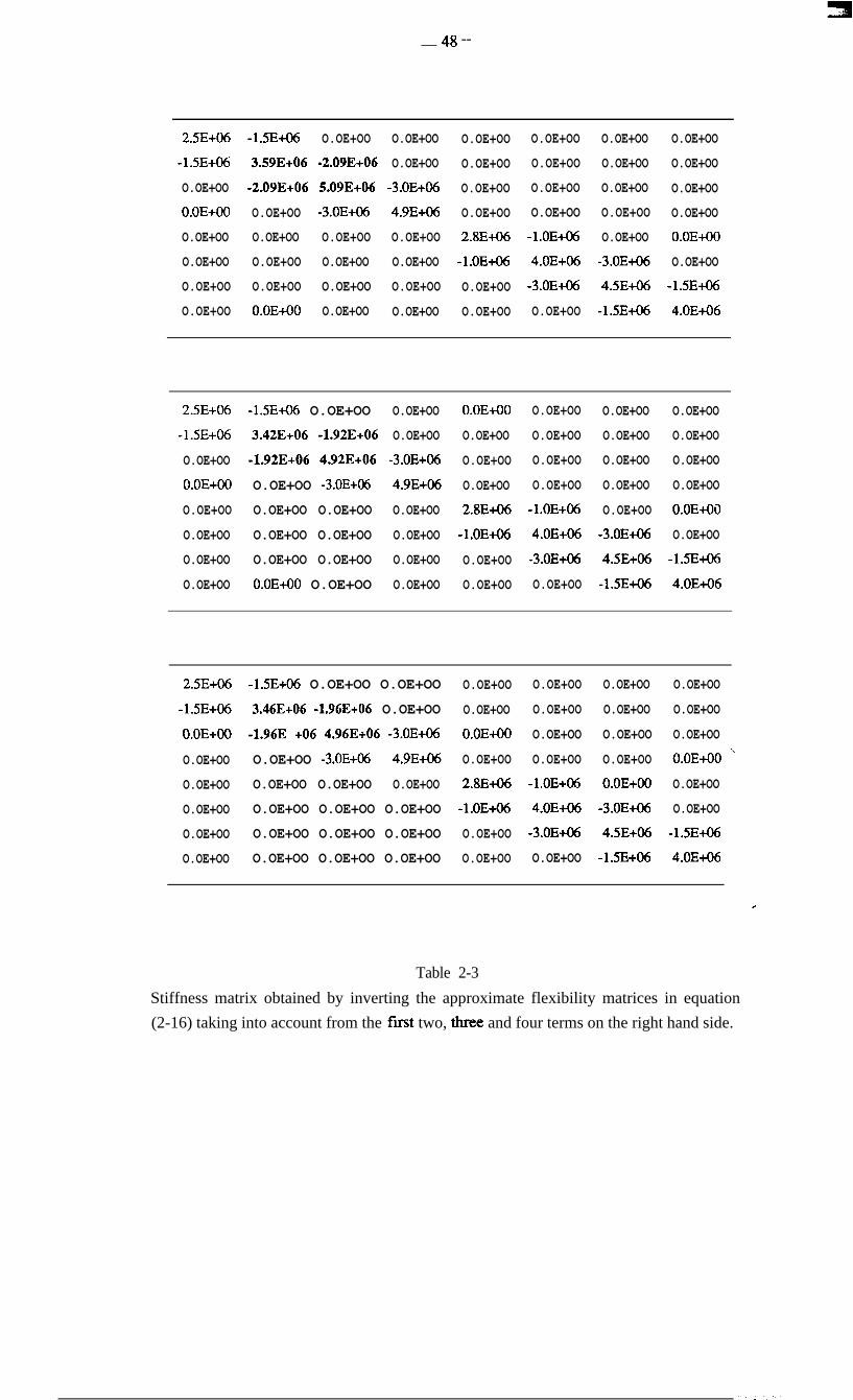
__ 48 --
2SE+O6
-1.5E+O6
O.OE+OO
O.OE+OO
O.OE+OO
O.OE+OO
O.OE+OO
O.OE+OO
-1SE+O6
3.593+06
-2.09E+06
O.OE+OO
O.OE+OO
O.OE+OO
O.OE+OO
O.OE+OO
O.OE+OO
-2.09E+06
5.093+06
-3.OE+O6
O.OE+OO
O.OE+OO
O.OE+OO
O.OE+OO
O.OE+OO
O.OE+OO
-3.OE+O6
4.9E+O6
O.OE+OO
O.OE+OO
O.OE+OO
O.OE+OO
O.OE+OO
O.OE+OO
O.OE+OO
O.OE+OO
2.8E+O6
-1.OE+O6
O.OE+OO
O.OE+OO
O.OE+OO
O.OE+OO
O.OE+OO
O.OE+OO
-1.OE+O6
4.OE+O6
-3.OE+O6
O.OE+OO
O.OE+OO
O.OE+OO
O.OE+OO
O.OE+OO
O.OE+OO
-3.OE+O6
4SE+O6
-1.5E+O6
O.OE+OO
O.OE+OO
O.OE+OO
O.OE+OO
O.OE+OO
O.OE+OO
-1.5E+O6
4.OE+O6
2.5E+O6
-1.5E+O6
O.OE+OO
O.OE+OO
O.OE+OO
O.OE+OO
O.OE+OO
O.OE+OO
-1.5E+O6 O.OE+OO
3.42E+06 -l.923+06
-l.92E+O6 4.92E+06
O.OE+OO -3.OE+O6
O.OE+OO O.OE+OO
O.OE+OO O.OE+OO
O.OE+OO O.OE+OO
O.OE+OO O.OE+OO
O.OE+OO
O.OE+OO
-3.OE+O6
4.9E+O6
O.OE+OO
O.OE+OO
O.OE+OO
O.OE+OO
O.OE+OO
O.OE+OO
O.OE+OO
O.OE+OO
2.8E+O6
-1.OE+O4
O.OE+OO
O.OE+OO
O.OE+OO
O.OE+OO
O.OE+OO
O.OE+OO
-LOE+O6
4.OE+O6
-3.OE+M
O.OE+OO
O.OE+OO
O.OE+OO
O.OE+OO
O.OE+OO
O.OE+OO
-3.OE+O6
4.5E+O6
-1.5E+O6
O.OE+OO
O.OE+OO
O.OE+OO
O.OE+OO
O.OE+OO
O.OE+OO
-1.5E+O6
4.OE+O6
2.5E+O6
-1.5E+O6
O.OE+OO
O.OE+OO
O.OE+OO
O.OE+OO
O.OE+OO
O.OE+OO
-1.5E+O6 O.OE+OO O.OE+OO
3.46E+06 -1.96E+06 O.OE+OO
-1.96E +06 4.963+06 -3.OE+O6
O.OE+OO -3.OE+O6 4.9E+O6
O.OE+OO O.OE+OO O.OE+OO
O.OE+OO O.OE+OO O.OE+OO
O.OE+OO O.OE+OO O.OE+OO
O.OE+OO O.OE+OO O.OE+OO
O.OE+OO
O.OE+OO
O.OE+OO
O.OE+OO
2.8E+O6
-1.OE+O6
O.OE+OO
O.OE+OO
O.OE+OO
O.OE+OO
O.OE+OO
O.OE+OO
-1.OE+O6
4.OE+O6
-3.OE+O6
O.OE+OO
O.OE+OO
O.OE+OO
O.OE+OO
O.OE+OO
O.OE+OO
-3.OE+O6
4.5E+O6
-1.5E+O6
O.OE+OO
O.OE+OO
O.OE+OO
O.OE+OO '
O.OE+OO
O.OE+OO
-lsE+O6
4.OE+O6
c
Table 2-3
Stiffness matrix obtained by inverting the approximate flexibility matrices in equation
(2-16) taking into account from the fust two, three and four terms on the right hand side.

__ 49 __
o.ooooo 0.00000
O.OOOOO 363677.
O.OOOOO -363677.
O.OOOOO 0.00000
O.OOOOO 0.00000
O.OOOOO 0.00000
O.OOOOO 0.00000
O.OOOOO 0.00000
O.OOOOO
-363677.
363677.
O.OOOOO
O.OOOOO
O.OOOOO
O.OOOOO
O.OOOOO
O.OOOOO
O.OOOOO
O.OOOOO
O.OOOOO
O.OOOOO
O.OOOOO
O.OOOOO
O.OOOOO
O.OOOOO
O.OOOOO
O.OOOOO
O.OOOOO
O.OOOOO
O.OOOOO
O.OOOOO
O.OOOOO
O.OOOOO
O.OOOOO
O.OOOOO
O.OOOOO
O.OOOOO
O.OOOOO
O.OOOOO
O.OOOOO
O.OOOOO
O.OOOOO
O.OOOOO
O.OOOOO
O.OOOOO
O.OOOOO
O.OOOOO
O.OOOOO
0.00000
0.00000
0.00000
0.00000
0.00000
0.00000
0.00000
0.00000
O.OOOOO 0.00000 O.OOOOO
O.OOOOO 83147. -83147.
O.OOOOO -83147. 83147.
O.OOOOO 0.00000 O.OOOOO
O.OOOOO 0.00000 O.OOOOO
O.OOOOO 0.00000 O.OOOOO
O.OOOOO 0.00000 O.OOOOO
o.ooooo 0.00000 O.OOOOO
O.OOOOO
O.OOOOO
O.OOOOO
O.OOOOO
O.OOOOO
O.OOOOO
O.OOOOO
O.OOOOO
O.OOOOO
O.OOOOO
O.OOOOO
O.OOOOO
O.OOOOO
O.OOOOO
O.OOOOO
O.OOOOO
O.OOOOO
O.OOOOO
O.OOOOO
O.OOOOO
O.OOOOO
O.OOOOO
O.OOOOO
O.OOOOO
O.OOOOO
O.OOOOO
O.OOOOO
O.OOOOO
O.OOOOO
O.OOOOO
O.OOOOO
O.OOOOO
0.00000
0.00000
0.00000
0.00000
0.00000
0.00000
0.00000
0.00000
O.OOOOO 0.00000 O.OOOOO
O.OOOOO 3172. -3172.
O.OOOOO -3172. 3172.
O.OOOOO 0.00000 O.OOOOO
O.OOOOO O.OOOOO O.OOOOO
O.OOOOO 0.00000 O.OOOOO
O.OOOOO 0.00000 O.OOOOO
0.00000 0.00000 O.OOOOO
O.OOOOO
O.OOOOO
O.OOOOO
O.OOOOO
O.OOOOO
O.OOOOO
O.OOOOO
O.OOOOO
O.OOOOO
O.OOOOO
O.OOOOO
O.OOOOO
O.OOOOO
O.OOOOO
O.OOOOO
O.OOOOO
O.OOOOO
O.OOOOO
O.OOOOO
O.OOOOO
O.OOOOO
O.OOOOO
O.OOOOO
O.OOOOO
O.OOOOO
O.OOOOO
O.OOOOO
O.OOOOO
O.OOOOO
O.OOOOO
O.OOOOO
O.OOOOO
0.00000
0.00000
0.00000
0.00000
0.00000
0.00000
0.00000
0.00000c
Table 2-4
[AK] for Case 1, obtained by repeatedly using equation (2-18)
e ,
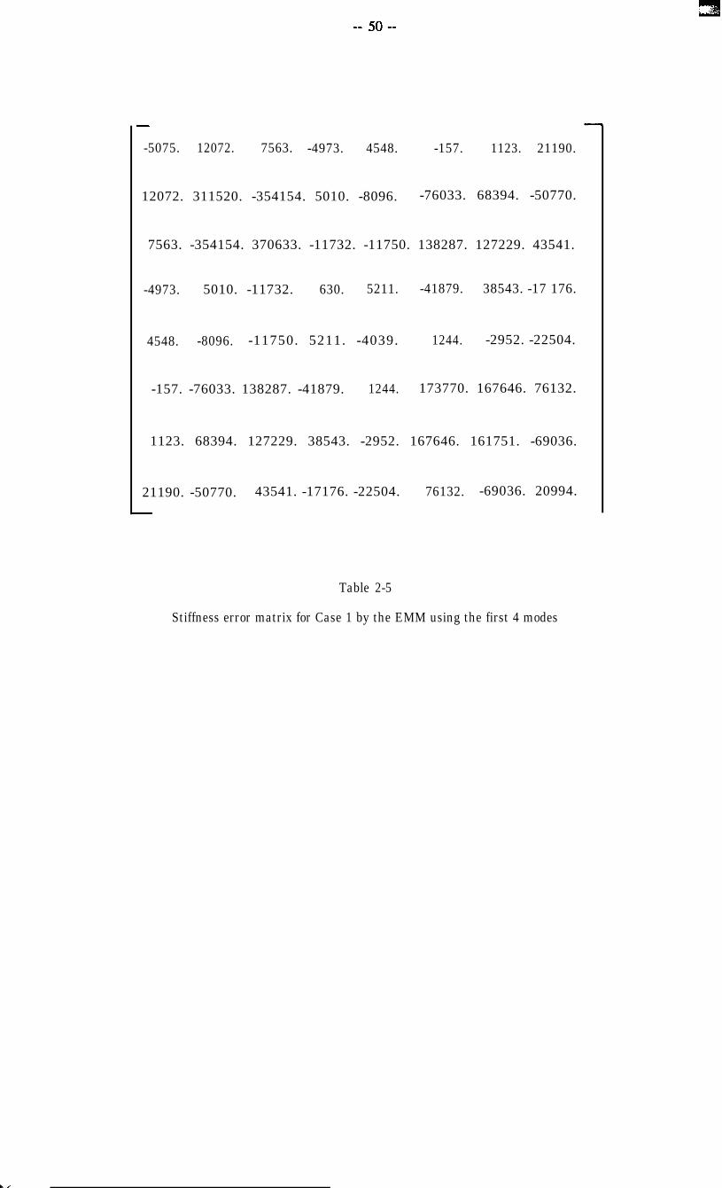
-
-5075. 12072. 7563. -4973. 4548. -157. 1123. 21190.
12072. 311520. -354154. 5010. -8096. -76033. 68394. -50770.
7563. -354154. 370633. -11732. -11750. 138287. 127229. 43541.
-4973. 5010. -11732. 630. 5211. -41879. 38543. -17 176.
4548. -8096. -11750. 5211. -4039. 1244. -2952. -22504.
-157. -76033. 138287. -41879. 1244. 173770. 167646. 76132.
1123. 68394. 127229. 38543. -2952. 167646. 161751. -69036.
21190. -50770. 43541. -17176. -22504. 76132. -69036. 20994.
Table 2-5
Stiffness error matrix for Case 1 by the EMM using the first 4 modes
I,

__ 51 __
Mode No. 1 2 3 4 5 6 7 8
Nat. Freq.Hz 21.373 33.858 78.452 89.864 103.423 212.566 296.473 406.767
X l
x2
x3mode
x4ShapeS
x5
x6
x7
x8
.07057 xx3130 .05016 .05977 .12481 .22656 .5rn16 .80582
.07373 .01#8 -DE67 26796 25354 30933 .36546 -.38938
06631 -.05485 .14783 .03574 28551 .13239 -.26471 .07730
.04279 -.03918 .20808 .10846 .10775 -.32322 .10084 -.01170
-.04571 -.05066 .03370 .0865 1 .13254 .22928 .52365 .80923
-.06263 .04423 .21387 -.03252 .2489 1 .33844 .40893 -.40756
-.06325 .07242 .15945 .11500 26519 .12384 -.27473 .08122
-.02595 .03320 -.04266 -.03719 .29410 -.33922 .10193 -.01164
Vibration modes for the analytical model of Case 1
Mode No. 1 2 3 4 5 6 7 8
Nat. Freq.Hz 21.384 34.443 79.597 93.286 103.494 213.326 303.898 410.018
xl .06989 .08018 .05977 .05086 .12412 .21841 -56229 .77958
x2 .07284 Xl0282 .04372 .26106 .244% .29917 .36014 -.40978
x3 .06700 -.05084 .14785 .02759 28540 .13883 -.25943 .08887mode
x4 I14324 -.03673 .22139 .07998 .10615 -.32638 .09066 -.01314shapes
x5 -XI4563 -.05329 .05016 .07670 .13098 .22107 .56596 .78284
x6 -05277 .04561 .21024 -.07046 .25604 .32209 .39508 -.42654
x7 -.06349 .07418 .17019 .10602 26163 .13174 -.26746 LB244
x8 -.02606 .033% -.05188 -.01579 .29418 -34245 .09140 -.01305 )
Vibration modes for the experiemntal model of Case 1
Table 2-6
All analytical and experimental vibration modes for Case 1
. c

__ 52 __
ModeNo. 1 2 5
before 0.054 1.699 1.439 3.668 0.069 0.356 2.443 0.793after 0.000 0.000 0.000 0.000 0.095 0.365 2.468 0.797
Percentage frequency errors
ModeNo. 1 2 3 8 total
before 0.728 5.764 10.86 19.18 1.368 3.181 5.279 4.514 50.87after 0.000 0.000 0.000 0.000 0.642 3.369 5.332 4.486 13.83
Percentage mode shape errors
Table 2-7
Percentage errors before and after the model is improvedby the CMM using the first 4 experimental modes
ModeNo. 1 2 3 4 5 6 7 8
before 0.054 1.699 1.439 3.668 0.069 0.356 2.443 0.793after 0.009 0.281 0.225 0.114 0.187 0.413 2.773 0.886
Percentage frequency errors
ModeNo. 1 2 5 8 total
before 0.728 5.764 10.86 19.18 1.368 3.181 5.279 4.514 50.87after 0.108 0.917 3.403 34.51 6.251 3.828 5.956 5.003 59.97
Percentage mode shape errorsc
Table 2-8
Percentage errors before and after the model is improvedby the EMM using the first 4 experimental modes

__ 53 --
2.5E+O6
-1.5E+O6
O.OE+OO
O.OE+OO
O.OE+OO
O.OE+OO
O.OE+OO
O.OE+OO
-1.5E+O6
3.00E+06
-150E+O6
O.OE+QO
O.OE+OO
O.OE+OO
O.OE+OO
O.OE+OO
O.OE+OO
-lsOE+06
4.503+06
-3.OE+06
O.OE+oO
O.OE+OO
O.OE+OO
O.OE+OO
O.OE+OO
'O.OE+OO
-3.OE+06
4.93+06
O.OE+OO
O.OE+OO
O.OE+OO
O.OE+OO
O.OE+OO
O.OE+OO
O.OE+OO
O.OE+OO
2.8E+O6
-l.OE+O6
O.OE+OO
O.OE+OO
O.OE+OO
O.OE+OO
O.OE+OO
O.OE+OO
-1.OE+O6
4.OE+O6
-3.OE+O6
O.OE+OO
O.OE+O
O.OE+OO
O.OE+OO
O.OE+OO
O.OE+OO
-3.OE+O6
4.5E+O6
-1.5E+O6
O.OE+OO
O.OE+OO
O.OE+OO
O.OE+OO
O.OE+OO
O.OE+OO
-1.5E+O6
4.OE+O6
Analytical stiffness matrix
2.5E+O6
-1.5E+O6
O.OE+OO
O.OE+OO
O.OE+OO
O.OE+OO
O.OE+OO
O.OE+OO
-1.5E+O6
3.45E+06
-1.95E+06
O.OE+OO
O.OE+OO
O.OE+OO
O.OE+OO
O.OE+OO
O.OE+OO O.OE+OO
-l.95E+O6 O.OE+OO
4.753+06 -2SE+06
-2.8E+O6 4.7E+O6
O.OE+OO O.OE+OO
O.OE+OO O.OE+OO
O.OE+OO O.OE+OO
O.OE+OO O.OE+OO
O.OE+OO
O.OE+OO
O.OE+OO
O.OE+OO
2.8E+O6
-1.OE+O6
O.OE+OO
O.OE+OO
O.OE+OO
O.OE+OO
O.OE+OO
O.OE+OO
-1.OE+O6
4.OE+O6
-3.OE+M
O.OE+OO
O.OE+O
O.OE+OO
O.OE+OO
O.OE+OO
O.OE+OO
-3.OE+O6
4.5E+O6
-1.5E+O6
O.OE+OO
O.OE+OO
O.OE+OO
O.OE+OO
O.OE+OO
O.OE+OO
-1.5E+O6
4.OE+O6
Experimental stiffness matrix
Table 2-9
Simulated analytical and experimental stiffness matrices for Case 2

__ 54 __
Mode No. 1 2 3 4 5 6 7 8
Nat. Freq.Hz 21.373 33.858 78.452 89.864 103.423 212.566 296.473 406.767
xl
x2
x3mode
x4shapes
x5
x6
x7
x8
.07057 .08130 .05016 .05977 .12481 .22656 .52016 .80582
.07373 .01048 -.00267 .26796 .25354 .30933 .36546 -.38938
.06631 -.05485 .14783 .03574 28551 .13239 -.26471 .07730
.04279 -.03918 .20808 .10846 .10775 -.32322 .10084 -.01170
-.0457 I -.05066 .03370 .0865 1 .13254 .22928 .52365 .80923
-.06263 .04423 .21387 -.03252 .2489 1 .33844 .40893 -.40756
-.06325 .07242 .15945 .11500 26519 .12384 -.27473 .08122
-.02595 .03320 -.04266 -.03719 .29410 -.33922 .10193 -.01164
Vibration modes for the analytical model of Case 2
Mode No. 1 2 3 4 5 6 7 8
Nat. Freq.Hz 21.314 34.428 79.411 93.203 102.684 210.721 302.901 409.954
X l
x2
mode
shapes
x3
x4
x5
x6
x7
x8
.06991 .08023 .05787 .04678 .12727 .20900 .56453 .78043
.07328 SKI272 .04137 .25358 .25431 .28997 .36685 -.40960
SE782 -.05110 .14243 .01794 .29096 .14051 -.25630 .08786
.04267 -.03621 .22214 .07650 .10725 -.32802 .08502 -.01230
-.04527 -.05354 .04833 .07248 .13473 .21160 .56824 .78369
-.06239 .045 16 .20443 -.07982 .25980 .3 1193 .40230 -.42634
-.06313 .0737 1 .16551 .09659 .27005 .13451 -26476 XI9147
-.02589 .03372 -.05512 -.02046 .28827 -3479 1 Al8665 -.01235
Vibration modes for the experimental model of Case 2
Table 2- 10
All analytical and experimental vibration modes for Case 2

__ 55 __
k-aY
22 23 (32) 33 34 (43) 44
iteration No.
0 87.0 76.9 94.7 107.1 104.3
: 96.3 89.1 94.1 61.4 99.8 85.1 102.9 92.0 101.8 99.48 96. I 77.7 93.3 96.6 100.1
12 95.6 79.4 96.6 100.4 101.516 95.1 77.6 97.0 100.7 101.620 95.9 78.3 98.1 101.6 101.9
Table 2- 11Percentage ratios of elements of stiffness matrices (k-(‘j/k-) %
(Direct iteration using the first four modes in Gale 2) ”
k --1Jiteration No.
22 23 (32) 33 34 (43) 44
0 87.0 76.9 94.7 107.1 104.3
i8
121620
96.9 93.6 99.0 95.9 97.897.8 96.0 99.0 100.6 100.597.8 96.0 99.1 100.8 100.697.8 96.0 99.2 101.0 101.697.8 96.0 99.3 100.7 101.797.8 96.1 99.3 101.1 101.7
Table 2-12
Percentage ratios of elements of stiffness matrices (kg(‘)/kij) %(Direct iteration using the first six modes in Case 2)
Y

__ 56 __
1 II;i
w
W
iAf
W
La L‘0\
c

__ 57 --
1
Incomplete Completeexperimental model analytical modelU$,lt @,I) [M,], [Kal (bt,ls b,l)
Error Matrix Methodb to calculate
stiffness error matrix
Modifyanalytical model
Yes I
Yes Not v
Improvedanalyticalmodel
Iterationfailed
Figure 2-3 Iteration process to improve an analytical model
c

-- 58
using First 2 modes
using First 6 modes
using First 8 modes
using First 4 modes
using First 6 modes
using First 8 modes
c
Figure 2-4 Stiffness error matrix [AK] for Case One, estimated by the CMM(left-hand side) and the EMM (right-hand side) using first 2,4,6 and
8 modes respectively.

,Dd
0”;b’.oo 2.00 4 -00 6 . 0 0 6 . 0 0 lb.00 12.00 14.00 lb.00 lb-00
Figure 2-5 Percentage of total mode shape errors for Case Two aftereach iteration using the EMM with the first 4 modes.
71
!2 - 00
c
Figure 2-6 Percentage of total mode shape errors for Case Two aftereach iteration using the EMM with the first 6 modes.


__ 61 __
CHAPTER 3
LOCATION OF MISMODELLED REGIONS
- NEW DEVELOPMENTS
3-l PRELIMINARIES
It was noted in the last Chapter that when the number of modes for which data are
available is insufficient - a situation which is very likely in practice - techniques such as
the CMM and the EMM might not successfully serve the purpose of locating errors in the
analytical model. It was also found that using an iteration process directly in an attempt to
improve the analytical model may end up with an unsatisfactory result. In fact, the
iteration often diverged from the expected answer. This is mainly because the information
contained in the measured modes is rather limited and it is over-demanding to try to
correct the whole analytical stiffness or mass matrix.
Although one has to accept the fact that the modes available for the attempt can be very
limited, it is also generally accepted that errors in the analytical model are normally
localised or isolated rather than spread throughout the whole model, since the FE
technique has been highly developed and computer facilities nowadays are sophisticated.
It is therefore believed that the major errors in the model should be located before an
attempt is made to improve the analytical model. If this location were successful, then the 4
model could be improved locally and this would be much more efficient. The attempt by
the CMM or the EMM to improve the whole analytical mass or stiffness matrix using only
a limited number of modes is not physically realistic.

__ 62 --
3-2 STRUCI’URAL CONNECI’MTY IN AN ANALYTICAL MODEL
The first and intuitive attempt to locate errors is to use the structural connectivity defined
by the analytical model itself. As described above, the structural connectivity inherent in
the analytical model should generaIly be respected during the model improvement and
hence this provides an obvious form of localization. As far as the stiffness properties are
concerned, this suggests that errors - if there are any - can only occur in the non-zero
elements of the analytical stiffness matrix [K,]. It is known that theoretically the
experimental stiffness matrix which is normally a banded matrix can be derived from the
modal data and the correct mass matrix, provided they are available:
(3-l)
To simulate the practical case where only the first m modes are available, the experimental
stiffness matrix can be taken to consist of two parts, including the first m modes and the
(3-2)
(3-3)
These two matrices can be shown schematically in Figure 3-l. Although neither is a
banded matrix, when be put together they will form the banded matrix [K.J. Normally,c
only matrix [K,]r can be determined from experimental modal data due to the
incompleteness of the measured modes. However, it can be said that all the elements in
matrix [KJ, which do not fall in the area band defmed by the structural connectivity in
w,] are supposed to be the errors because of the insufficient modes used and they will be
. , .I..

__ 63 __
changed into zeros if more and more modes are involved. Therefore, those elements
violating connectivity should be suppressed artificially, as in Figure 3-2, since they are
known to be zero. The iteration process can therefore be applied with the connectivity
requirement imposed as the means of error location, albeit only approximate. Physically,
this implies that only those stiffness property changes physically allowed by the system or
structure will be accepted.
As previously explained, the CMM is an optimization approach and, therefore, is not
directly applicable as an iteration approach. However, if the connectivity could be
imposed on the optimized stiffness or mass matrix by the CMM, as described above, then
it will become possible to apply the CMM iteratively. Each time, the connectivity
suggested by the original analytical model is enforced onto the resultant mass or stiffness
matrices obtained by the CMM.
A number of numerical studies were carried out using the EMM and the CMM iteratively
with the connectivity condition being imposed each time on the improved analytical
stiffness matrix as described above. However, it is found that this refined iteration
procedure does not generally produce much improved results. In fact, in the case where
the number of modes used is limited, so that directly applying the EMM or the CMM to
update the analytical model tends to diverge, this new iteration considering the
connectivity was unsuccessful.
It can be said that by considering the connectivity we confine the errors to occur inside the
connectivity area. The philosophy of the approach is simply requiring the errors to be
such that they cannot violate the connectivity while it does not pinpoint exactly where they
are in the analytical model. If the errors existing in the analytical model could be located c
exactly, and the iteration process implemented merely to correct these errors, the
improved model would be desirable. The results in Chapter 2 have shown that, due to the
limited number of modes, the EMM or the CMM could not exactly locate the errors and
direct iteration could not succeed either, so that a new technique needs to be developed to

enable the exact error location using limited number of modes and to facilitate the iteration
with this exact error location.
$3 LOCATION OF MISMODELLED REGIONS IN THE ANALYTICAL MODEL
3-3-l The Analytical Stiffness Case
It is generally believed that in most practical cases the mass properties of a vibration
structure are somewhat easier to model than are the stiffness properties. As a result, the
analytical mass matrix is generally acceptably accurate due to the highly sophisticated
theoretical modelling techniques used and so, when the stiffness matrix case is
investigated here, it is hence presumed that the analytical mass matrix is the same as the
experimental one ([M,]=[MJ). Any areas in the analytical stiffness matrix where errors
exist are generally small and local compared with the whole matrix and these areas are
called “mismodelled region(s)” here. The aim becomes to pinpoint these regions using the
limited number of measured modes when existing techniques do not effectively serve that
purpose.
According to definition, the stiffness error matrix is:
[AK1 = W,l - [&I (3-4)
Equation (3-4) can be post-multiplied on both sides by the incomplete measured mode
shape fnatrix [Q.J, leading to:
[AK][@J = I&] [+,I - &] [+,I (3-5) ,
Although the experimental stiffness matrix [KJ is unknown, so that the right hand side of
equation (3-5) cannot be specified, the measured modal data should satisfy the following
relationship,

__ 65 __
vq [$,I = [qJ E~,l bx2.1 (3-Q
where the mass matrix N] here could be replaced by the accurate analytical mass matrix
so that the right hand side of equation (3-6) consist of all known matrices. Thus,
substituting equation (3-6) into equation (3-5) yields:
[AK][+x] = [MaI [9,1[~w,2.1 - fKal[%l (3-7)
Post-multiplying both sides of equation (3-7) by the transpose of the incomplete measured
mode shape matrix, [$,I, leads to:
[AK] ([$,I [(&IT) = [MaI NJ [y2.1 [@,lT - [Kal hxl[@,lT) (343)
It is clear that matrix ([$X][Q,]T) cannot be inverted to obtain the stiffness error matrix
[AK], because the mode shape matrix [@,I does not contain all the modes and is rank
deficient. However, it is of considerable interest to note that matrix product in the left
hand side of equation (3-8) happens to provide an indication of the mismodelled regions,
and this matrix product can be derived from the right hand side of the equation which
consists of all known matrices. This is explained further in the following.
Equation (3-8) can be transposed to become:
(NJ [$JT)Wl = [@,I [*~:.I [~JTIMal - ([~,IhP,lT)[Kal (3-9)
and both equations (3-8) and (3-9) are illustrated in Figure 3-3. Since it is supposed that
the mismodelled region(s) in [K,] is usually a local and isolated area, this region can be4
represented in Figure 3-3 as a small shaded area on the left hand side. It is clear that
equation (3-8) indicates the rows in [KJ which contain errors. Since the stiffness
matrices [K,] and [KJ are usually symmetrical, as is matrix [AK], equation (3-8) has
actually located the mismodelled region. In common with equation (3-8), equation (3-9)

__ 66 __
shows the columns in matrix [K,] which contain errors and consequently locates the
r&modelled region. Therefore, the n&modelled region can be located by either using
equation (3-8) to locate the rows in [KJ containing errors or equation (3-9) to locate the
columns in [K,] containing errors. It will be visually more obvious to add these two
equations to form the results shown in Figure 3-4, where the overlapped area indicates
exactly where is the mismodelled region of the stiffness matrix.
Further examination reveals that equation (3-5) and its derivatives can be written using as
few as just one measured mode { Cp,); (i=l, 2, . . . N) at a time, rather than all the available
measured modes [QJ, giving:
(3- 10)
Following the same procedure of matrix manipulation from equations (3-5) to (3-8) leads
to:
(3-l 1)
Equation (3- 11) shows that only one measured mode is needed as far as the location of
the mismodelled region is concerned, provided that this mode is vibrationally sensitive to
[AK]. Thus, the location of the mismodelled regions in [K,] can be performed by using
any one of the measured modes or combination of the measured modes and this provides
the error location with an alternative indication which could make the location process
more reliable.c
It should be noted that throughout the development of the theory above, there is no
assumption that matrix [AK] is small necessary to qualify the feasibility of the theory.
This is unlike the cases of the EMM or other methods. Although the theory here

__ 67 __
obviously cannot be used to update the matrix [I&] by any kind of iteration process -
rather, it can only be employed to locate the errors from [KJ using the measured mode(s)
- it is clear that the location of the mismodelled regions is the primary concern for the
model improvement study in most times and it has been shown above that the model
improvement could hardly be effective or sensible if this location is not provided
3-3-2 The Analytical Mass Case
The same methodology as described in the last section can also be applied to the mass
matrix case where a mass error matrix [AM] exists. In practice, it can be said that cases
where the analytical mass matrix is less reliable than the stiffness matrix are relatively
rare. As far as the joints between the components of a structure are concerned, stiffness
modelling errors are expected to be much more serious than those for the mass. However,
there are still some practical structures for which the mass modelling could be technically
very demanding and the credibility of the resultant analytical mass matrix may be
questioned.
In a similar way to the last section, this analysis first presumes that the analytical stiffness
matrix is acceptably accurate so that it can be taken as the same as the experimental one
([K,]=[KJ) when the mass matrix case is investigated. Also, the area(s) in the analytical
mass matrix where errors exist is generally small and local compared with the whole
matrix and such areas are similarly called “mismodelled region”. The aim becomes the
pinpointing of these regions using the limited number of measured modes available.
The mass error matrix is defined as:
[AMI = IMJ - [MaI (3-12)
Equation (3-12) can be post-multiplied on both sides by the incomplete measured mode
__ 68 __
shape matrix [@,I and the natural frequency matrix [++2.1, leading to:
[AMI [$,I [*q2.1 = [&I N,l bx2.1 - [Ma1 [@,I b’x2.1
Substituting equation (3-6) into equation (3-13) will lead to:
(3-13)
(3- 14)
post-multiplying equation (3-14) on both sides by the transpose of the mode shape matrix
[$,I will finally yield:
[AMI ([O,l[~w~.l [$,lT) = [&I [OxI I$xlT - [Mal([@xl [‘ax2.1 [(&IT) (3-15)
The right hand side of equation (3-15) consists of known matrices. Compared with
equation (3-8), it is found that this equation provides a significant indication of the
mismodelled region(s) in the analytical mass matrix, although the matrix product
([~,][~x~.][$,]~) cannot be inverted to obtain [AM] directly. If equation (3-15) is
transposed, giving:
([+,I [*@;.I [4+lThW = [$,I [~,fKJ - ([$,I W:.l M,lT)CMal (3-16)
then, combining equations (3-15) with (3-16) will indicate the r&modelled regions in
[MJ clearly and can be presented pictorially in Figure 3-4, as for the stiffness case.
of copse, equation (3-15) can dso be written using any one of the measured modes,
yielding:c
Again, the location of the mismodelled regions in [M,] can be performed by using any

__ 69 __
one of the measured modes or different combinations of measured modes and this
provides the error location with multiple references which could make the location more
reliable.
3-3-3 General Case
The stiffness matrix and mass matrix cases have been investigated separately in the last
two sections. In reality, however, a combined situation may well occur and the
mismodelled regions in both [K,] and [M,] need to be located simultaneously using the
mode shapes from measurement. In this case, the premise of [M,]=[M,] for equation
(3-7) is no longer applicable and equation (3-12) should be substituted into equation (3-7)
to deal with this problem. This leads to:
[AK]]@,] = ([Ma1 + Wl)[~xl[‘~x2.1 - [K,l[+xl (3-18)
Post-multiplying both sides of this equation by the transpose of the measured incomplete
mode shape matrix [$,,I yields:
Wl([@J [@,lT) - [W([@J bx2.1 [@JT)
= [MJ( [$,I b&l b&lT) - [K,l @l @,lT) (3-19)
Equation (3-19) may also be obtained by substituting equation (3-4) into equation (3-14).
Akin to equations (3-8) and (3-15) to locate the mismodelled regions in [K,] andc
MJseparately, equation (3-19) facilitates the error location in the same way. However,
the complication involved here is the coexistence of [AK] and [AMJ and equation (3-19)
only provides the location of the mismodelled regions in the analytical model. Therefore,
it is to be identified from the results of equation (3-19) which error region is caused by

__ 70 __
[AK] and which by [AM].
3-4 DIRECI’ NUMERICAL CALCULATION OF [AK]
In addition to revealing mismodelled regions in the analytical mass and stiffness matrices,
the advantage of the location technique proposed in the previous section is that it offers
the possibility of estimating [AK] (or [AMJ) by immediate numerical calculation, provided
the number of measured modes is sufficient. It is believed that the errors in the analytical
model are often local and isolated while, without the effective error location, the model
could normally be updated artificially everywhere in such a way that the resultant model
would severely violate the structural connectivity and dramatically alter the physical
properties in a way which is not practically sensible or acceptable. However, instead of
simply applying methods such as the EMM and the CMM to end up with this undesirable
new model, the measured modes may well be adequate to quantify these local and isolated
errors, once they have been localized, and the analytical model can be updated in a way
which not only preserves the connectivity but also presents the correct dynamic
characteristics of the system or structure without sacrificing the physical properties.
This section investigates the implementation of this numerical calculation. Only the [AK]
case is dealt with here and it is presumed that the analytical mass matrix [M,] is correct
and hence [M,] is used in following formulations when w,] occurs in the analysis. The
principle is equally valid for estimation of [AMJ
Using one measured mode (Cp,)i (instead of the set, [+,]>, equation (3-7) becomes: i
[WI (Cp,)i = CO,2>ilM~l ((P,)i - lKJ(TxIi (3-20)
The right hand side of this equation consists of known quantities. If it is supposed, for
c I
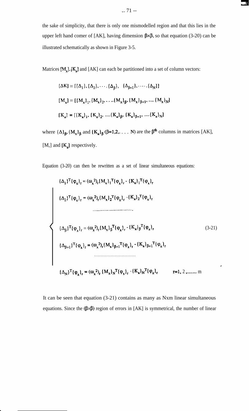
_- 71 --
the sake of simplicity, that there is only one mismodelled region and that this lies in the
upper left hand comer of [AK], having dimension pxp, so that equation (3-20) can be
illustrated schematically as shown in Figure 3-5.
Matrices [MJ, [K,] and [AK] can each be partitioned into a set of column vectors:
[AK1 = [(AIL IA2L . . . . {A$, (AB+l), . . . . . (AN}]
[M,l = HMJ,, IMx12v . . ..W& (Mx}p+l’ .-+- ($&I
[KJ = [IKJ,, Wa12. -{K,Jp~ {Ka)p+1’ -.tKa)~l
where (A)B, {M,)P and {K,lP @=1,2,. . . . N) are the p” columns in matrices [AK],
[M,] and [K,] respectively.
Equation (3-20) can then be rewritten as a set of linear simultaneous equations:
{41TIq9, = (q),~~12T(cp,~, - K~2T~cp,)r
. . . . . . . . . . . . . . . . . . . . . . . . . . . . . . .
{Ap]T{~,], = (c@,{&]pT&‘,,, - IK,]bT@,]r
{A~+t)T{~,], = (W,2),(&]p+tT((Px]r - (K,]p+rT(qx]r
. . . . . . . . . . . . . . . . . . . . . . . . . . . . . . .
(3-21)
c{ANJToX), = (w:)~ (M,INT((P,]r - {KahT((J’,), t=l, 2 ,......... m
It can be seen that equation (3-21) contains as many as Nxm linear simultaneous
equations. Since the (pxp) region of errors in [AK] is symmetrical, the number of linear

__ 72 __
simultaneous equations required for numerical determination of [AK] is only p@+l)/2 out
of the total number of Nxm in equation (3-21), provided these equations are independent
one another. As each mode can produce up to p linear simultaneous equations, this means
the number of measured modes required is reduced to @+1)/2 - which is relatively small.
However, further algebra reveals that the linear simultaneous equations in (3-21) are not
independent. Further, it is concluded that only p modes are needed in order to obtain the
[AK] by solving the first p linear simultaneous equations numerically.
It will naturally be the case in practice that more than one localized mismodelled region in
[K,] has to be dealt with. For instance, suppose that there are two such regions, as shown
in Figure 3-6, having dimensions (pxp) and (cxxa) respectively. Since the two non-zero
regions can be dealt with separately in terms of the numerical calculation described above,
the number of modes needed to obtain matrix [AK] will still be p, provided here a<p.
3-5 NUMERICAL ASSESSMENT OF LOCATION TECHNIQUE AND
REFINED ITERATION PROCESS
The location of the mismodelled regions in an analytical model by a limited number of
measured vibration modes is, in most cases, the primary goal since it pinpoints the failure
of the theoretical analysis and provides the analyst with useful information of which part
of the structure or system needs to be carefully reanalysed. On the other hand, once the
mismodelled regions in the analytical model have been successfully located, the analytical
model can also be improved by the available measured modes using existing techniques
such as the iterative EMM. Unlike the direct iteration procedure introduced earlier this
time only the localized regions in the analytical model will be modified while the
remaining major parts in the model can be kept unchanged. Figure 3-7 shows the strategy
of this refined iteration process to improve an analytical model. It can be said that this

__ 73 --
refined iteration is physically more sensible than the direct iteration applied in the last
chapter which tends to modify the whole analytical model.
The dynamic system used to assess the location technique introduced here is the same as
that used in the last chapter. The two case studies investigated there are studied further
here: the system description and corresponding simulated analytical model and the
experimental modes being as in the last Chapter.
The mismodelled region in the analytical stiffness matrix [KJ will then be located using
the new technique developed in this chapter. Once the region has been accurately located,
a refined iteration process similar to that direct iteration used in the last Chapter and the
slightly improved iteration introduced in the beginning of this Chapter can be used. The
refinement for this new iteration process will be in conjunction with the proposed location
results and will include restriction of any changes in matrix [IS,] to the mismodelled
region which has been located. Any other changes (beyond the localized region) indicated
by the results of EMM or the CMM will be regarded as errors caused by the
incompleteness of the experimental modes and will not be admitted.
Case Study 1 The simulated analytical and experimental stiffness matrices used in this
study are for the system shown in Figure 2-l and are the same as those shown in Table
2-1, and the simulated experimental modes are in Table 2-6. The actual stiffness error
matrix is shown in Figure 2-2 and indicates a mismodelled region in the analytical
stiffness matrix. Equation (3-l 1) can be used to locate this mismodelled region and Figure
3-8 shows the results of using equation (3-l 1) with a single mode at a time - from mode 1
to mode 8 - and it can be seen that each mode locates errors on rows 2 and 3 of matrix .
F.-J, indicating errors on elements 2,2; 2,3; 3,2; 3,3 of the matrix - which are, in fact,
exactly in the mismodelled region. Comparing Figure 3-8 with Figure 2-4 indicates that
the location technique suggested in this chapter is much more accurate and efficient and
requires considerably fewer experimental modes than other existing methods.

__ 74 --
Case Study 2 The simulated analytical and experimental stiffness matrices in this study are
the same as those shown in Table 2-7 while the corresponding simulated experimental
modes are in Table 2-8. In order to locate exactly the mismodelled region in matrix [K,],
equation (3-l 1) is used in turn with each mode individually, as in Case Study 1. Figure
3-9 shows the results of using equation (3-l 1) with single mode each time (from modes 1
to 4) and it can be seen that the result for each mode locates the same mismodelled region
- on elements 2,2; 2,3; 3,2; 3,3; 3,4; 4,3; 4,4 of matrix [KJ - it can also be seen from
Table 2-7 that this located region is correct.
Since the mismodelled region in matrix [K,] has been successfully located, the iteration
process can then be carried out to improve the analytical model by updating matrix [K,,].
This time, only the localized region in the original matrix [K,] will be modified by the
results of the EMM or the CMM using the first four modes (the same as the case studied
in Chapter 2). The total mode shape error is then recorded in Figure 3-10 and the ratios of
elements of stiffness matrices are presented in Table 3-1. It can be seen by comparing
Figure 3- 10 with Figure 2-7 and Table 3-l with Table 2-9 that using this refined iteration
process on the same case as before shows significant advantages over using direct
iteration. Furthermore, a much faster rate of convergence to the correct solution has been
achieved than that when only the connectivity was considered.
3-6 CONCLUSIONS
Since the number of vibration modes which can be measured on practical structures is c
likely to be limited, the corresponding analytical model cannot usually be corrected by a
simple application of either the EMM or the CMM, because the results violate the
connectivity of the analytical model and could be unacceptably approximate. Under these
circumstances, the iteration process is introduced, seeking to improve the analytical model

iteratively and to produce an eventually satisfactory result. This direct iteration process
was found in the last chapter to be relatively unsuccessful for model improvement since
the iteration can hardly converge to the correct answer.
A first attempt to improve the iteration process was made by applying the connectivity
requirements of the analytical model. It is noted that the improved or corrected analytical
model must preserve the connectivity of the original model, based on a physical view of a
vibration system the model describes. The results of the EMM and the CMM (which
violate connectivity each time in the iteration process) are errors due to the insufficiency of
the number of measured modes (and other approximations incurred) and should not be
taken into account in the model improvement. This slightly improved iteration process has
been assessed numerically but has not given convincing results. A possible reason for the
relative lack of success of this refined iteration process is that even when connectivity is
preserved, the model improvement still implies that all the non-zero stiffness (and/or
mass) properties theoretically predicted are erroneous and it tends to “improve” the whole
of the analytical model (albeit preserving the connectivity conditions).
It is concluded that difficulties in constructing an analytical model for the vibration
properties of a structure are generally encountered only in some local parts of it due to
sophisticated analytical modelling techniques now available. Therefore, errors in an
analytical model are generally localised and can be referred to as “n-&modelled regions” in
the analytical model. A sensible model improvement procedure should thus seek to
modify these mismodelled regions only, rather than to improve the whole analytical
prediction. Hence, an exact location of these mismodelled regions from the analytical
model is crucial.
Considering the practical situation where the number of measured modes is very limited,
and the current methods such as the EMM or the CMM cannot always locate the
mismodelled regions in a clear-cut way, a new method has been proposed in this chapter
which enables the location to be made with a very limited number of measured modes

(even with only one measured mode). The method is successfully evaluated using the
same test cases as before in contrast to less successful location using conventional
techniques. It is also proposed in this chapter that if the number of modes is greater than
the dimension of the mismodelled region (or the dimension of the biggest mismodelled
regions if there are more than one), the exact model correction can be carried out by
numerical calculation.
The iteration process to improve the analytical model can now be refined, once the
mismodelled regions have been exactly located in the analytical model. Only these
mismodelled regions are modified each time in the iteration process by repeatedly using
the measured vibration modes. The results have shown marked advantages over those for
direct iteration, or for iteration considering connectivity constraints only. It is therefore
suggested that the analytical model improvement should be carried out in this way.
c

__ 77 __
kij
22 23 (32) 33 34 (43) 44
Iteration No.
0 87.957 76.923 94.737 107.143 104.255
1 96.300 94.408 99.786 102.920 101.758
4 100.073 99.65 1 100.026 100.195 100.171
8 100.066 99.767 99.839 99.969 99.964
12 100.060 99.795 99.839 99.855 99.952
16 100.054 99.8 14 99.852 99.873 99.955
20 100.049 99.831 99.90 1 99.878 99.959
Table 3- 1
Percentage ratios of elements of stiffness matrices (kijWkij) %
(Location and iteration using the first four modes in Case 2)
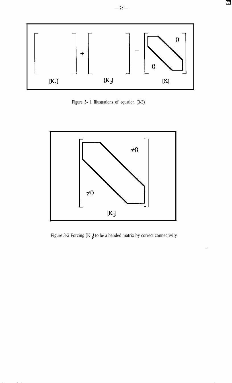
__ 78 __
Figure 3- 1 Illustrations of equation (3-3)
Figure 3-2 Forcing [K J to be a banded matrix by correct connectivity
c
,. -

__ 79 --
tzlWI
hm#dT
[$I NIT
ElWI
I1
.
1Figure 3-3 Illustrations of equations (3-8) and (3-9)
1 r- 1
Figure 3-4 Location of the mismodelled region in [AK]
I ,

__ 80 __
Figure 3-5 Schematical presentation of equation 3-21when only one mismodelled region exists
lsl PXP
q axa
WI
,
Figure 3-6 Schematical presentation of equation 3-21 when
more than one mismodelled region exist

_- 81 --
Incompleteexperimental model analytical model[~J rqJ W,l, WJ @#‘,I, b&
Location ofMismodelled regions using
[$,J, bxl and [&I. [K J
I
Error Matrix Methodto calculate
stiffness error matrix
analytical model
Yes 1
Yes No
+
Improvedanalyticalmodel
t
Iterationfailed
c
Figure 3-7 Refined iteration process to improve an analytical model

-- 82 __
Figure 3-8 Location of stiffness error for Case One using experimental
modes from 1 to 8 individually.
. : -_

-- 83 __
Figure 3-9 Location of stiffness error for Case One using experimental
modes from 1 to 4 individually.
- .--

__ 84 __
Figure 3- 10 Percentage of total mode shape errors for Case Two after eachiteration using the EMM and the stiffness error location results.


__ 86 --
CHAPTER 4
IDENTIFICATION OF DAMPING PROPERTIES
OF VIBRATING STRUCTURES
4-1 PRELIMINARIES
In the previous Chapters, the location of r&modelled regions in an analytical model and
the subsequent model improvement using measured vibration modes have been dealt
with. When a structure is lightly damped, the vibration modes identified from
measurement are often regarded technically as real modes, and it has been suggested that
the mismodelled regions can be located effectively by using just a few measured modes.
Moreover, once those regions have been successfully located, the analytical model
improvement can be focussed in the located regions with the iterative process often
producing convincing results which are physically sensible (in contrast to the less
convincing results of conventional techniques in many cases).
However, some practical structures are more heavily damped and the measured modal
data in such cases are sometimes no longer real. This provokes difficulty in applying the
theory discussed in the last two Chapters for investigating the analytical model. Besides,
theoretical modelling cannot generally predict the damping properties in detail and so the
most likely form for a damping matrix is one which is ‘proportional’ to the mass and/or c
stiffness properties, in which case the analytical vibration modes are still real. Although
this proportional damping model can readily be applied theoretically, it rarely represents
the correct damping properties of real structures.

__ 87 __
There have been a number of approaches reported in the literature[28]-[32] which seek to
deduce the undamped vibration modes from the measured damped complex modes so that
the deduced real modes could be used to modify the erroneous analytical stiffness or mass
matrix. In that case, the new development in the previous chapters could be applicable for
error location from an analytical model and for the subsequent model improvement.
However, the undamped modes thus deduced are often merely a rough approximation
since the experimentally identified complex modes are essentially incomplete and the
deduction itself relies to some extent on the analytical model which is erroneous.
Furthermore, these approaches are not applicable to the location of the damping elements
in a structure since they stand on extracting the undamped modes and, in the process,
throw away that information concerning the damping properties. It is therefore thought
that the experimentally identified complex modes could be used in order to locate the
damping elements.
The identification of dynamic characteristics of a damped structure becomes more
complicated due to the fact that the erroneous analytical model is to be modified at the
same time as the damping properties remain to be investigated. It is believed that it would
be possible to investigate the damping properties when the analytical stiffness matrix is
relatively accurate. However, this Chapter will consider the general case, i.e. when the
structure is damped and its analytical stiffness matrix is in error, and suggests that it is
possible to locate the mismodelled regions in the stiffness matrix and meanwhile to locate
the damping elements. It will also be shown that the iteration process followed by a
successful location could convincingly quantify the damping matrix and the errors
existing in the analytical stiffness matrix separately.
4-2 CURRENT APPROACHES FOR Sl-‘UDWG DAMPING PROPERTIES c
The damping properties of a practical structure are perhaps the most difficult aspect to
investigate, compared with the mass and stiffness characteristics. The difficulty results
mainly from the the fact that the damping in a vibrating structure cannot be specified by

__ gg --
analytical methods in the same precise way as can the mass and stiffness characteristics.
For some lightly damped structures, the theoretical modelling often assumes them to be
undamped and for other cases, where the damping existence cannot be ignored, a linear
and proportional damping model is often used. This theory suggests that distribution of
damping in a structure takes the same form as that of the mass or stiffness (or both)
properties, hence the hysteretic damping matrix N or viscous damping matrix [C] could
be described by:
WI = dK1 + PM1 (4-l)o r
[Cl = r[Kl + 6Dfl (4-2)
The notable advantage of using this proportional damping model is that the mode shapes
of a structure with such damping are identical to the corresponding undamped model and
the natural frequencies will be just slightly different. (It is of interest to note that
proportional damping models defined by equations 4- 1 and 4-2 are not the only cases to
produce the identical modes with the undamped ones and the more general condition is
discussed in literature[28]). However, due to the increasing complexity of the dynamic
structures to be studied and more stringent demands on the analytical models to include an
accurate damping matrix, this assumption of proportional damping becomes less and less
appropriate to cope with practical applications.
It is believed that the nature and extent of the damping present in most practical structures
can only be determined by experiment. Indeed, measured modal data which come from a
successful measurement contain “true” information about the damping properties of a
structure. To investigate the information on the damping properties from measurement, it
is supposed that the dynamic characteristics of the vibrating structure can be described by ,
a discrete multi-degree-of-freedom system whose equations of motion are as be10w[~~]:
(-w2[Mx] + [KJ+i[HJ){q}eia = {F)eiO’ (4-3)
where it is presumed that the damping is of the hysteretic type and (q} is a vector of
complex harmonic amplitudes. Or, in case of the other widely used damping type -

__ gg __
viscous damping - the equations of motion will be:
(-w~[M,] + wi[C] + [KJ){q]eiU = (F}eiat (4-4)
Under the circumstance of single point excitation, the receptance of the system between
points “j” and “k” with hysteretic or viscous damping can be defmed respectively by:
ajkf$k + ‘Pjk
I=1 1 - (oJw,)2 + Q,
ajk& + i(o/o,)~j~
r=l 1 - (o/o,)2 + 2i(o/o,)5,
(4-5)
(4-6)
where A, B are the real and imaginary parts of the modal “constant”.
Information about the damping properties is contained in the complex modal constant, the
natural frequency Or (which slightly differs from the undamped natural frequency) as well
as the damping loss factor r\, (or h). The major drawbacks of this information are: (1) it
is normally insufficient because of the incompleteness of the measured modal data and,
(2) it does not explicitly yield the damping distribution in the structure.
If, in any case, only a few damped vibration modes rather than a representative damping
model are of interest in a given practical application, then these damped modes can
generally be identified experimentally to fulfil the requirement. However, as far as the
stringent demands on the analytical models are concerned to include the damping matrix,
the incomnlete damping information revealed by the measured modes are certainly not
straightforward to enable it. In the literature, effort has been paid to the derivation of a
damping matrix directly from a limited number of measured modes[34]-[38] as well as to
derive the mass and stiffness matrices. Such derivation may be appropriate in the cases
where the vibration characteristics of a structure will be defined only by the
experimentally-specified number of coordinates and the same number of modes.
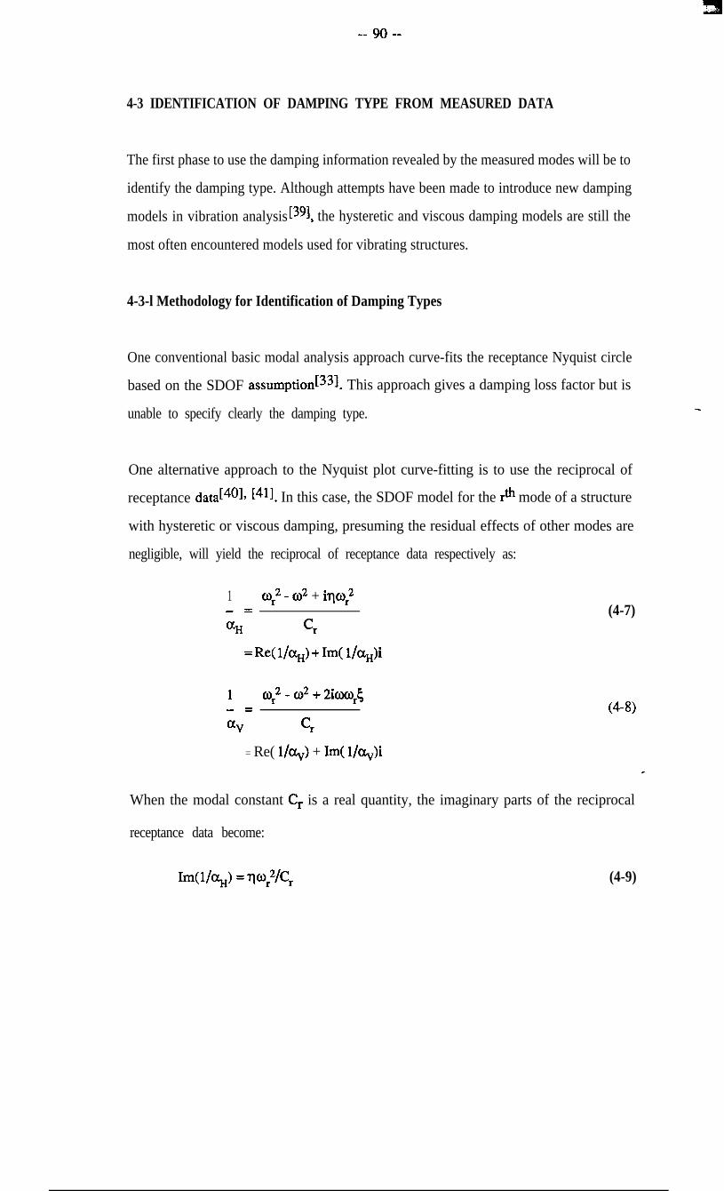
__ go --
4-3 IDENTIFICATION OF DAMPING TYPE FROM MEASURED DATA
The first phase to use the damping information revealed by the measured modes will be to
identify the damping type. Although attempts have been made to introduce new damping
models in vibration analysis [391, the hysteretic and viscous damping models are still the
most often encountered models used for vibrating structures.
4-3-l Methodology for Identification of Damping Types
One conventional basic modal analysis approach curve-fits the receptance Nyquist circle
based on the SDOF assumption[ 331. This approach gives a damping loss factor but is
unable to specify clearly the damping type.
One alternative approach to the Nyquist plot curve-fitting is to use the reciprocal of
receptance data[ 40]v i41]. In this case, the SDOF model for the r* mode of a structure
with hysteretic or viscous damping, presuming the residual effects of other modes are
negligible, will yield the reciprocal of receptance data respectively as:
1 o2 + iqq2- =aH Cr
= Re( l/aH) + h( l/aH)i
(4-7)
(4-Q
c
1 cor2 - a2 + 2ic06$- =% Cr
= Re( l/o+) + Im( l/cxv)i
When the modal constant Cr is a real quantity, the imaginary parts of the reciprocal
receptance data become:
(4-9)

__ 91 __
or Im( l/cQ = 2w,w5/C,
In a plot of the imaginary part of l/a against frequency o (Figures 4-la and 4-lb), these
two damping types are indicated by either a horizontal line for hysteretic damping or a
straight line with non-zero slope for viscous damping. Equations (4-9) and (4- 10) are the
basis of the identification of damping types.
The simplicity of thus identifying the type of damping is, however, sometimes
undermined by the practical situation in which we can hardly rely on the modal constant
from the measured data to be real, especially when the damping magnitude is significant.
The complexity of the modal constant, as often exists, will tend to mix the real and
imaginary parts of the receptance data and hence the reciprocal of the receptance data will
not be so directly able to identify the damping type. In order to identify the damping when
the mode is complex, it is now proposed that the complexity of the modal constant can be
removed once its phase angle is accurately identified by Nyquist circle curve-fitting.
4-3-2 Removal of Complexity from Measured Data
A complex modal constant can be written as the expression in equations (4-7) or (4-8)
multiplied by a complex number (cosCl+isine) with unity modulus. The effect of the
complexity of the modal constant in the Nyquist circle will thus be to rotate the whole
circle from the original position by an angle 8, as illustrated in Figure 4-2. Hence, the
reciprocal of the receptance data with a complex modal constant is given as:
l/cc = Re(l/a) + Im(l/a)i
= [Re( l/a) + Im( l/&i] [(co& - isine)] (4-11)
where IQ is referred to as the receptance when the modal constant is real.
.

__ 92 __
Thus, it can be thought that the measured data are in such a form that a set of receptance
data with no complexity are transformed by a complex quantity with unity modulus and
so the measured data could be subjected to equation (4-l 1). The phase angle 6 in equation
(4- 11) may be deduced by the Nyquist circle curve-fitting and, consequently, the purely
real and imaginary parts (before being transformed by the complexity) can be deduced
from equation (4- 1 l), being respectively:
Re( l/m> = Re( l/a)cose - Im( l&sine
Im( l/m> = Im( l/a)cost3 + Re( l&sine(4- 12)
Thus, data Im(l/& can be used to identify the damping type, as described above.
4-4 LOCATION OF DAMPING ELEMENTS FROM A STRUCI’URE
441 Usual Damping Condition of a Vibrating Structure
From the point of view of modal analysis, the damping properties of a vibrating system
defined by equations (4-3) or (4-4) can be specified by the system’s modal data (i.e. by
the damped natural frequencies, complex modal contansts and, above all, the damping
loss factors) in equations (4-5) or (4-6) respectively. However, these modal data are not
directly related to the spatial distribution of damping in the system. For instance: given a
damping matrix, the modal data (especially those damping loss factors which most
significantly reflect the damping properties) will change if there is a change in the stiffness
matrix. As has been discussed in the last two Chapters, the theoretically-predicted
stiffness matrix will generally contain errors, and so the damping properties indicated by
the modal data should be treated with considerable care.c
Fortunately, unlike the mass and stiffness characteristics which are generally contributed
to by all parts of a structure, the most significant damping in structures usually comes
from the joints between the various components [42lJ431. In other words, it can be said
that damping mainly occurs at or between a restricted number of coordinates in terms of

__ 93 __
the analytical model, and so the usual assumption of proportional damping will not
satisfactorily cope with such practical cases. Figure 4-3 shows schematically a damping
matrix which could be regarded as representing a ‘true’ damping matrix case for a
practical structure.
Hence, it is supposed that useful information about the damping distribution in a structure
could be revealed by localizing the damping elements in a vibration model determined
from measurements, such as those obtained from a modal test. If the damping elements
can be successfully localized by the measured data, then the damping matrix of the
corresponding analytical model of the structure will be provided in an acceptable form,
similar to that in Figure 4-3, rather than conventionally assuming it to be proportional to
the mass and stiffness matrices as in equations (4-l) and (4-2), and any further attempt to
quantify the damping level could be directed to those local&d elements.
4-4-2 The Approach for Damping Element L+ocation
When hysteretic damping exists in a vibrating structure, it is generally accepted that the
damping matrix [Hj can be combined with the stiffness matrix [K,J (or [KJ if it comes
from the analytical model and is with errors) to form what is called ‘complex stiffness
matrix’, (as was introduced in Chapter 3):
&I = l&l + ilKI (4-13)
For the sake of simplicity, it is first assumed that the mass and stiffness properties of the
analytical model of the structure are acceptably accurate when the location of damping
elements from the structure is investigated and, hence, the stiffness matrix [Kx] in 0
equation (4-13) can be adequately represented by the analytical stiffness matrix. The more
general case, with an erroneous analytical model, will be considered later. Since the
structure is damped, its measured vibration modes will be complex and the mode shape
matrix, denoted by [+,I, will be incomplete with less than all the modes included.

__ 94 __
Equation (4 13) can be post-multiplied by the complex mode shape matrix [+,I, yielding:
[&I [OxI = [&I N,l + i[HJ M,l
Since the following relationship holds for the experimental model,
(4- 14)
&I [@,I = W,l [@,I [‘@;.l (4-15)
it can be substituted into equation (4-13) to eliminate the unknown complex stiffness
matrix [K,] and, by rearranging and post-multiplying the resultant equation on both sides
by the transpose of the measured complex mode shape matrix [QJT, yields:
(4-16)
In common with the approach developed in Chapter 3 to locate the mismodelled regions in
the mass and stiffness properties of the analytical model, equation (4- 16) can be used in a
similar way to locate the damping of the structure by pinpointing the significant elements
in the damping matrix. It should be noted that the incomplete measured mode shape
matrix [@,I and the measured natural frequency matrix [‘wx2.] are both complex while the
structure’s stiffness, mass and damping matrices are all real. With this in mind, equation
(4-16) can be split into two equations, representing its real and imaginary parts
respectively. It is the imaginary part of equation (4-16) which enables the location of the
damping by pinpointing the significant elements in the damping matrix [III. Moreover,
equation (4-16) can be written using as few as just one measured complex mode to cope
with the practical situation when the number of measured complex modes could be strictly
limited. z
As mentioned earlier, a complication of damped structures lies in the argument that the
analytical model is erroneous when the damping properties remain to be investigated. It is
believed that it would be somewhat easier to investigate the damping properties when the

__ 95 __
analytical stiffness matrix is effectively accurate. However, to consider the general case,
when the analytical stiffness matrix is not correct, equation (4-13) will become:
&I = [Kal+[~Kl+ UII (4-17)
The derivation from equation (4- 13) to equation (4 16) will now yield:
[AK] [@,I [ (&IT + i[Eil [@,I b&IT = M,J NJ [*~~~.l [$JT - FJ[$JhlT (4-18)
Comparison of equation (4-18) with equation (4-16) indicates that equation (4-18) tends
to locate the mismodelled regions in the analytical stiffness matrix and the damping
elements simultaneously. Theoretically, when equation (4-18) is split into its real and
imaginary parts, the effects of [AK] and [HJ will show up in both and it is thought that
closer inspection of the structure might be helpful in order to identify the non-zero parts in
[AK] and [HI from the results of equation (4-18). However, it can generally be expected
that the effect of [AK] will dominate the real part of equation (4-18) and that of [HJ the
imaginary one. Again, equation (4-18) can be written using as few as only one measured
complex mode. The application of equation (4-l 8) will be presented later in this chapter.
4-5 EZXIMATION OF DAMPING MATRIX
4-S-l Extension of the EMM to Estimate Damping Matrix
Once the significant elements in the damping matrix IHJ have been localized, the attention
of the damping property investigation is consequently turned to the possible evaluation of
the damping matrix itself using the limited number of measured complex modes available.
Although the standard EMM (Chapter 2) is available to estimate the stiffness or mass error ’
matrices [AK] or [AM], there is no corresponding technique to estimate the damping
matrix and the following paragraphs develop the EMM in order to facilitate the damping
matrix estimation.

For generality, the analytical stiffness matrix [K,] (assumed to be derived from an FE
analysis, or similar) is taken to be erroneous, albeit only slightly. The error is denoted in
Chapter 2 as [AK], is called ‘the stiffness error matrix’ and is usually small compared
with [K,]. It is convenient to define here a complex stiffness error matrix [AKJ which is
the difference between the correct complex stiffness matrix in equation (4-13) (which is,
in practice, unavailable) and the (real) analytical stiffness matrix, i.e.:
[A&l = [&I - WJ (4-19)
= UK,1 + WI) - <&I - WI)
= [AK] + i[HJ (4-20)
The real part of this complex stiffness error matrix [AK,] is effectively the stiffness error
matrix defined by the EMM in Chapter 2 while the imaginary part of [AK,] represents the
damping matrix.
From equation (4-19), the correct complex stiffness matrix [K,] can be written as:
WC1 = @,I + [AK,1
Inverting both sides leads to:
[KJ-’ = tl&l + WJ)-’
= ( El + [~al-‘[~cIY1[~al-l
= t [II - WJ-‘WC11 + Wal-‘[~,l)2 - . . . . .HKJ-’
= [KJ-’ - ([KJ’[AKJ)[K,]-’ + ([KJ-‘[AKJ)2[KJ-’ - . . . . . (4-21) c
Since matrices [AK] and [H] can be assumed to be small compared with [K,], similar
validation to that used in Chapter 2 shows that matrix product ([KJ’[AK,])” approaches

__ 97 --
a zero matrix as n increases, i.e.:
([KJ1[AKC])* +[O] as n+w.
Then, equation (4-21) becomes:
[KC]-’ = [KJ-’ - [KJ-‘[AK,][K$’
so [&I-‘k=,I[KJ-’ = KJ-’ - KJ-’
and [AK, = [KJ ( KJ’ - [&I-’ ) KJ (4-22)
(4-23)
Since the real part of the complex stiffness error matrix [AKJ is defined as [AK], and the
imaginary part as [HI, equation (4-22) can be split into its real and imaginary parts to
yield both the stiffness error matrix and the damping matrix:
[AK] = Real ([AK,])
= RealI W,l ( W,l-’ - [KJ-’ 1 [&I 1
= [&I ( [KJ-’ - Red (KJ-'1 1 l&l
Wl = Irw WK,I)
= Imad EK,l ( &I-’ - l&l-’ 1 [KJ 1
= I&l Wag ([K,l-lIJ [&,I (4-24)
,
Equations (4-23) and (4-24) indicate that the stiffness error matrix [AK] and damping
matrix [HI can be estimated separately when they coexist. Estimation of the damping
matrix can thus be implemented by estimating the imaginary part of [AK,] only,

__ 98 __
In order to use an incomplete set of vibration modes to estimate the stiffness error matrix
[AK] and the damping matrix [III, the analytical flexibility matrix [KJ’ and the
experimental complex flexibility matrix [KC]-’ must be approximated by the
corresponding real and complex modal data:
[&I-’ = N+J _[~@I-‘_ MaITmxn
&I-’ = [$,I _[.q2J1 _ MxlTm m
(4-25)
(4-26)
Therefore, the stiffness error
equation (4-24) can be obtained
[AK] = Real ([AK,])
matrix in equation (4-23) and the damping matrix in
using the modal data as:
= EKJ ( [$,I ba2.1-' MJT - Red { [$JPo,2.1-’ [@,JT 1) &I (4-27)
WI = Imag WK,I)
= &I bag { l$JlI ‘q.l-‘M,lTl) l-&l (4-28)
It should be borne in mind that the damping matrix estimated by equation (4-28) will be a
full matrix, ‘predicting’ damping properties throughout the structure. This is due to the
limited number of modes available from measurement and is contradictory to the usual
damping condition of a vibrating structure as indicated above (i.e. damping concentrated
at relatively few points). It also needs to be noted that as the number of measured modes
increases, the significant elements in damping matrix [HJ will show up more and more c
clearly in the damping matrix estimated by equation (4-28) and such a trend could be an
additional means of confuming the damping element location suggested in $4-4.
One interesting feature in estimating the damping matrix is that close modes will play a

__ 99 --
significantly important part in the process. Since the damping matrix [H] is small
compared with [KJ, it can be regarded as a complex perturbation of [KJ. The complex
stiffness matrix [K,] (i.e. &]+i[Hj) is then the result of this perturbation. According to
perturbation theory, the consequence of a perturbation i[HJ on the stiffness matrix K] is
that each complex mode shape { $Jr (r=1,2 . . ..n) after perturbation can be expressed as a
combination of the corresponding real mode shape {Q,}, before perturbation Dlus a
contribution of all the other (real) mode shapes. Mathematically:
If two modes, r and s, are very close to each other, then, since (wf’ - os2) is small, they
will both contribute significantly to the change of each mode shape. This means that close
modes are likely to have a considerable effect in the perturbation i[Hl on [KJ and may be
expected to contain significant information of the perturbation on mode shapes so that
they will be especially effective in estimating the damping matrix. Therefore, the damping
matrix estimated using equation (4-28) will be more accurate if two measured vibration
modes are very close and are employed in the estimation.
4-5-2 Iterative Approach to Improve the Estimation of [HJ
Since the significant elements in the damping matrix [Kj can be localized before the
damping matrix itself is estimated by equation (4-28), the elements in [HJ estimated by
equation (4-28) which are not localized by means of the measured complex vibration
modes will be regarded as errors introduced by the insufficiency of the number of 0
measured modes and will be artificially suppressed, as used in the stiffness error matrix
case studied in Chapter 3. The same argument will be applied to the stiffness error matrix
[AK] estimated by equation (4-27). In addition, matrices m and [AK] thus estimated will
be expected to be rough estimates since the number of measured complex modes used will

__ 99 --
significantly important part in the process. Since the damping matrix [H] is small
compared with [KJ, it can be regarded as a complex perturbation of [KJ. The complex
stiffness matrix [K,] (i.e. &]+i[Hj) is then the result of this perturbation. According to
perturbation theory, the consequence of a perturbation i[HJ on the stiffness matrix &] is
that each complex mode shape { $JT (r=1,2 . . ..n) after perturbation can be expressed as a
combination of the corresponding real mode shape {Q,), before perturbation Dlus a
contribution of all the other (real) mode shapes. Mathematically:
If two modes, r and s, are very close to each other, then, since (of’ - os2) is small, they
will both contribute significantly to the change of each mode shape. This means that close
modes are likely to have a considerable effect in the perturbation i[Hl on [KJ and may be
expected to contain significant information of the perturbation on mode shapes so that
they will be especially effective in estimating the damping matrix. Therefore, the damping
matrix estimated using equation (4-28) will be more accurate if two measured vibration
modes are very close and are employed in the estimation.
4-5-2 Iterative Approach to Improve the Jlstimation of [HJ
Since the significant elements in the damping matrix [Kj can be localized before the
damping matrix itself is estimated by equation (4-28), the elements in [l!-IJ estimated by
equation (4-28) which are not localized by means of the measured complex vibration
modes will be regarded as errors introduced by the insufficiency of the number of 0
measured modes and will be artificially suppressed, as used in the stiffness error matrix
case studied in Chapter 3. The same argument will be applied to the stiffness error matrix
[AK] estimated by equation (4-27). In addition, matrices m and [AK] thus estimated will
be expected to be rough estimates since the number of measured complex modes used will

often be very limited. However, with the knowledge of the location results, this
estimation can be carried out iteratively with the limited number of measured complex
modes in order to achieve a reasonably accurate damping matrix. The process can be
illustrated as in Figure 4-4 and is subjected to a numerical case study below.
4-6 NUMERICAL ASSESSMENT OF DAMPING PROPERTY INVESTIGATION
A series of numerical studies were carried out in order to validate the technique proposed
above for locating the damping in a vibrating structure. Also, by examining the damping
matrix obtained using an incomplete set of measured vibration modes, an attempt is made
to produce an acceptable damping matrix for the structure based on the accurate damping
element location.
The system used for the numerical study was the same as that shown in Figure 2-l and
used in the previous two Chapters, with the exception that it is now supposed to
include
one hysteretic damper, with a value of 4.5~105 N/m, attached between coordinates 6 and
7, thus forming the system shown in Figure 4-5. The correct damping matrix for the
system is shown in Figure 4-6. Three damping cases are investigated:
(i) when the analytical stiffness matrix is reliable;
(ii) when the analytical stiffness matrix is erroneous and;
(iii) when close modes exist for the system.
These three cases are denoted as “Case Dl, Case D2 and Case D3” respectively. For all
the various cases investigated, the mass matrix remains unchanged (and correct).
Case Dl The stiffness matrix of the system is the same as the analytical stiffness matrix in
Table 2-l and is supposed to be correct. Thus, all 8 simulated ‘analytical’ modes and
‘experimental’ modes can be obtained by eigensolution. It should be noted that the
‘analytical’ modes are real and the ‘experimental’ modes are complex since the system is
now damped and the ‘analytical’ model does not include the damping properties. Table

-- lOl--
4-l presents all eight undamped and damped natural frequencies and damping loss
factors.
Equation (4-16) is applied to locatethe non-zero elements in the damping matrix [II’j. To
simulate the practical situation of having only a limited number of measured vibration
modes, and to assess the feasibility of the approach proposed in this Chapter, only one
simulated measured complex mode is used at a time in applying equation (4-16). Figure
4-7 provides graphical presentations of the location results obtained by equation (4-16)
using one mode at a time - from mode 1 to mode 4. This figure suggests that the damping
element can be located by using as few as one measured complex mode, provided this
measured mode is sensitive to the damper.
Case D2 To consider the more general practical situation, it is thought that the analytical
stiffness matrix will often be erroneous for a damped structure and hence, the case of
coexistence of [AK] and [II’J has to be investigated numerically in order to lend fully
support to the approach developed in this Chapter. To simulate this case, it is supposed
that the analytical and the experimental stiffness matrices are the same as Case 1
investigated in the previous two Chapters (Chapters 2 and 3) while the damping condition
is the same as for Case Dl above. The stiffness error matrix [AK] is then the same as that
in Figure 2-2. The objectives of this case study are first, to locate both the m&modelled
region in the analytical stiffness matrix between coordinates 2 and 3 and the damping
element between coordinates 6 and 7 and, second, to assess the possibility of determining
both [AK] and [IIJ accurately using the iterative process illustrated in Figure 4-4.
Table 4-2 presents the natural frequencies and damping loss factors for both undamped
analytical and damped “experimental” cases. It is interesting to note - by comparing Table
4-l with Table 4-2 - that the damping loss factors in these two cases are quite different
from each other, even though the damping distribution in the system is the same in both
cases. This supports the suggestion made in the early part of this Chapter that a given
damping matrix may not present a unique set of damping loss factors in the modal data,
c

-- 102 --
because the damping loss factors depend on mass and stiffness properties as well as the
damping distribution. However, it can be seen from the results detailed below that correct
damping element location will still be achieved.
To locate the mismodelled region in [KJ and the significant elements in [III, equation
(4-18) is used with any one of the measured complex modes. Figure 4-8 shows the
results of using equation (4-18) with just one mode at a time. The left-hand column in the
figure is the real part of equation (4- 18) and the right-hand column the imaginary part. It
is clear from this Figure that results from each application consistently pinpoint the correct
location of the stiffness errors in the analytical matrix [K,] (between coordinates 2 and 3)
and the damping element between coordinates 6 and 7.
Once the correct location for [K,] and [HJ has been achieved, equations (4-27) and (4-28)
can be used to calculate respectively the stiffness error matrix [AK] and the damping
matrix [HI. It is also attempted in this case study to assess the iterative process suggested
in Figure 4-4. Accordingly, the first four complex modes were used together in applying
equations (4-27) and (4-28) iteratively and for each iteration the results were modified in
accordance with the correct location already available. Figures 4-9 to 4-14 show the
natural frequency errors, the damping loss factor errors of all 8 modes, the total mode
shape errors of the real and imaginary parts of the mode shapes and the errors of each
mode shape. All the results indicate the notable success of the iteration process. The final
improved analytical stiffness matrix and the constructed damping matrix are considered to
be accurate enough, when compared with the correct stiffness and damping matrices.
Case D3 It can be seen from Tables 4-l and 4-2 that neither Case Dl nor Case D2 has any *
close modes (close in the sense of natural frequencies). To investigate the effect of close
modes on damping element location, the stiffness matrix of Case Dl is adjusted so that
the undamped and damped natural frequencies and damping loss factors are as shown in
Table 4-3. It can be seen that modes 4 and 5 are very close to each other in this new
-- 103 --
configuration and hence only these two modes are used in equation (4-28) to calculate a
damping matrix. The result shown in Figure 4-15 indicates clearly the dominance of these
two modes in estimating the damping element between coordinates 6 and 7 and confirms
that close modes can be decisive in investigating the damping properties of a vibration
system.
4-7 CONCLUSIONS
The difficulty of investigating the damping properties of a vibrating structure lies mainly
in two aspects (in addition to the inevitable practical situation of incompleteness in the
measured vibration modes): (1) the damping properties cannot be specified by analytical
methods in the same way as can the mass and stiffness characteristics, and (2) the
damping properties of a structure have to be investigated in many cases where the
analytical model of it is erroneous in the stiffness and/or mass properties as well.
It is expected that the damping properties of most vibrating structures are not distributed
in a similar way to the mass and stiffness, and so the conventional proportional damping
model is not appropriate to represent the true damping distribution. Rather, damping often
comes from the joints between the various components of a structure, or from the
structural failures such as internal cracks. Therefore, it believed to be more appropriate to
investigate the damping properties by first locating the major damping elements using the
measured complex vibration modes and then, if the number of measured vibration modes
is adequate, estimating the damping matrix based on the suggestion of a successful
damping element location.
It is believed that modal data from a successful measurement contain the necessary
information about the structure’s damping properties. However, the information provided
by the experimenta.l modal data does not reveal explicitly the spatial or global damping
distribution of the structure. Moreover, the information can be misinterpreted when the
erroneous analytical model of the structure is applied to investigate the damping

--104--
properties.
An analytical approach has been developed to locate the damping elements in a vibrating
system using a very limited number of measured complex vibration modes. Case studies
using the approach have demonstrated that the mismodelled regions in an analytical
stiffness matrix can be located by the real part of equation (4-18) while the damping
distribution is revealed by its imaginary part. Once a successful location has been
achieved for both [K,] and [HJ, improving matrix [KJ and estimating [HI can then be
implemented by using the extended EMM in a iterative process. Encouraging results
based on simulated data have been obtained that validate the analytical approach.
Furthermore, it has been found that close modes contain much more valuable information
about the complexity of the system than do isolated modes, suggesting that they are
especially important in methods for constructing the damping distribution. It is suggested
that the approach proposed in this Chapter is feasible in investigating the damping
properties of vibrating structures.
c

-- 105 --
UNDAMPED DAMPEDNATURAL NATURAL DAMPING LOSS
FRJZQURENCIES FREQUENCIES FACTORS
21.3729 Hz33.8582 Hz78.4522 Hz89.8641 Hz
103.4225 Hz212.5663 Hz292.4734 Hz406.7665 Hz
21.3729 Hz33.8756 Hz78.4983 Hz89.8756 Hz
103.4224 Hz212.7217 Hz296.6479 Hz406.5155 Hz
.ooooOJO776JO523.03052MI028.01140.06077.01643
Table 4-lNatural frequencies and damping loss factors for Case Dl
UNDAMPEDNATURAL
FREQURENCIES
DAMPEDNATURAL DAMPING LOSS
FREQUENCIES FACTORS
21.3729 Hz33.8582 Hz78.4522 Hz89.8641 Hz
103.4225 Hz212.5663 Hz292.4734 Hz406.7665 Hz
21.3834 Hz .0000134.4070 Hz .0077179.5351 Hz S-IO29393.0651 Hz .03648
103.4838 Hz .00005213.3700 Hz .00918303.3162 Hz .05499409.3685 Hz .01804
Table 4-2Natural frequencies and damping loss factors for Case D2
UNDAMPEDNATURAL
FREQURENCIES
DAMPEDNATURAL DAMPING LOSS
FREQUENCIES FACTORS
5.0029 Hz8.8321 Hz
20.3547 Hz24.0661 Hz25.5812 Hz51.6245 Hz79.9811 Hz
114.8575 Hz
5.0045 Hz .003758.8483 Hz .02667
20.3561 Hz .0004924.2047 Hz a440925.4991 Hz .0211551.6300 Hz XI027978.0000 Hz .04938
114.8295 Hz a0966
Table 4-3Natural fkquencies and damping loss factors for Case D3
-
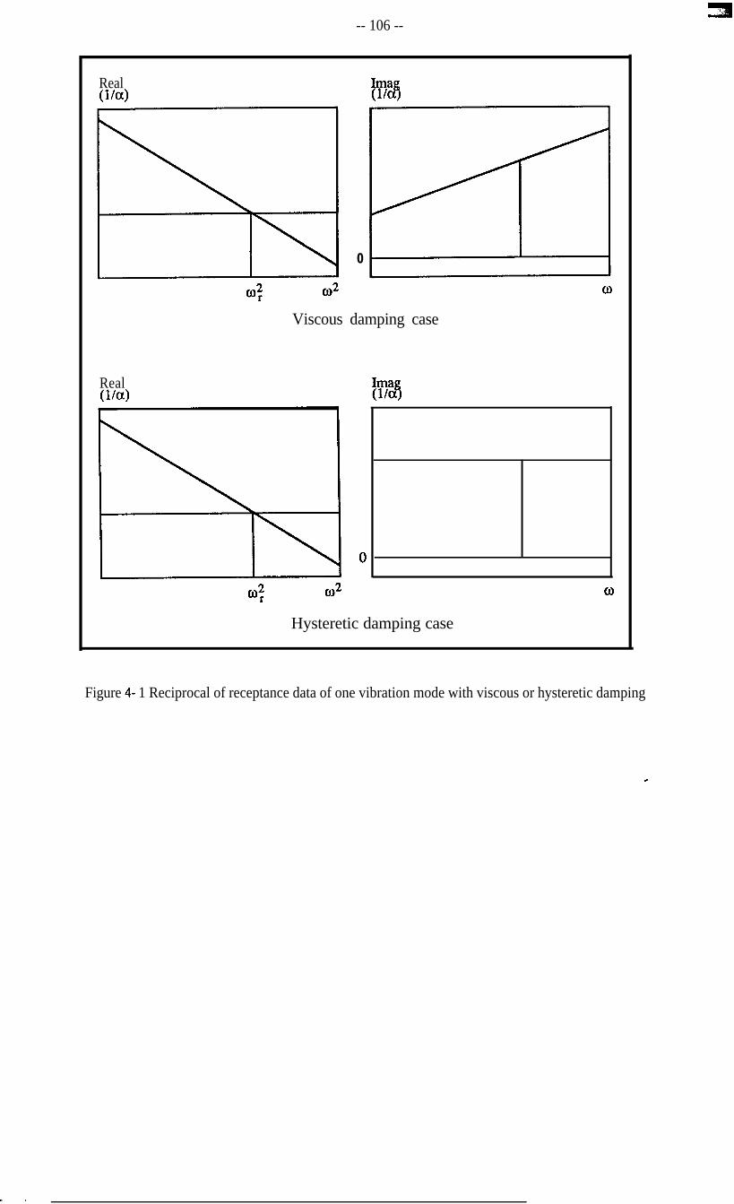
-- 106 --
RealWa)
0
63
Viscous damping case
Real(l/a)
4 co2 0
Hysteretic damping case
Figure 4- 1 Reciprocal of receptance data of one vibration mode with viscous or hysteretic damping
c

-- 107 --
Im I Im
Re
Figure 4-2 Rotate the Nyquist circle to remove the effect of complexity
.
Porportional damping matrix
L
Practical damping matrix
Figure 4-3 A typical practical damping matrix compared with a proportional damping matrix *
.

-- 108 --
1 Incomplete ComDlex 1 I Complete ti
t-i
experimental model analytical model
NJ, [ql W,l, D&J (N$,ls b$
*
Location forFKl and WI
I
Modify analytical model&
construct damping matrix
I
No
Yes I
Yes No
accurate [H]a&
Improvedanalyticalmodel
Iterationfailed
Figure 4-4 Iteration process to estimate [HJ and to improve [K,]
c

_ _. . _. -- _.
\
i-1xl II
L-
cx3 X
Figure 4-5 An 8DOF system with an incorrect stiffness componentand a theoretically unpredicted damper.
Figure 4-6 Correct damping matrix for the systemshown in Figure 4-5.

mode 1 only mode 2 only
mode 3 only mode 4 only
Figure 4-7 Graphical presentations of the location results for Case Dlusing equation (4-16) with modes from 1 to 4 individually.

Figure 4-8 Graphical presentations of the location results for Case D2 usingequation (4-16) with modes from 1 to 4 individually.Left-hand side columr\: location of stiffness errors.Rm location of damping elements.

-- 112 --
a..w
Figure 4-9 Percentage errors of all 8 natural frequencies for Case D2 after eachiteration using the EMM and the error location results.
-4-
a.4
.w
Figure 4-10 Percentage errors of all 8 damping loss factors for Case D2 after eachiteration using the EMM and the error location results.

-- 113 --#I6 I I I 1 1 I I I ‘
SId
?2d
d-00 I .oo 0.00 al.00 lb.00 lb.00 li.00~ lb.00 lb.00 I
Figure 4-l 1 Percentage of total mode shape errors (real parts) for Case D2 aftereach iteration using the EMM and the error location results.
I I I I I I I I I
,W
Figure 4- 12 Percentage of total mode shape errors (imaginary parts) for Case D2after each iteration using the EMM and the enw location results.

-- 114 --
Figure 4-13 Percentage errors of all 8 mode shapes (real parts) for Case Two aftereach iteration using the EMM and the error location results.
a6
8d
8%.w f.00 4.00 d.00 d.00 rb.oo 1k.00 $4.00 Il.00 lb.00 0
Figure 4- 14 Percentage errors of all 8 mode shapes (imaginary parts) for CaseTwo after each iteration using the EMM and the en-or location results.
I . _, , -6, I.

-- 115 --
Figure 4-15 Effect of two close complex modes in Case D3 in estimating
damping matrix using equation (4-28).

f

-- 117 --
CHAPTER 5
COMPATIBILITY OF MEASURED MODES AND
ANALYTICAL MODEL
5-l PRELlMINARJEs
As described earlier, the incompleteness of the set of the measured modes has two
aspects. First, the number of modes available from measurement (m) is usually very
limited (mcN) and second, the number of coordinates identifiable by measurement (n) is
less than the number of coordinates specified in the analytical model (n<N).
It has been shown in the earlier part of the thesis that, theoretically, the mismodelled
regions in an analytical model could be located from just a few measured modes using the
new approaches proposed in Chapters 3 and 4 when neither the basic EMM nor the CMM
are successful in doing so. However, the location of mismodelled regions can be
implemented only when the measured modes are compatible with the analytical mass and
stiffness matrices in terms of specified coordinates and, in the majority of cases, this
compatibility is not present.
Usually, an analytical model will employ a far greater number of coordinates to describe
the vibration characteristics of a structure than is practical for the measured data. The
reason for the measured modes to have a limited number of coordinates lies mainly on c
two counts: (1) vibration measurement is too expensive to permit testing many
coordinates and (2) some coordinates may be either technically difficult to test (such as
rotation coordinates) or physically inaccessible (such as those coordinates specified by the
analytical model which are ‘inside’ the structure). Experience has shown that modal tests
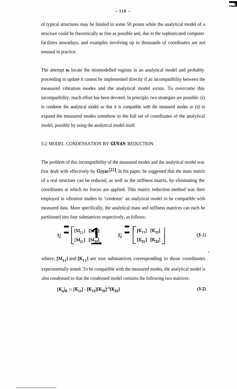
-- 118 --
of typical structures may be limited to some 50 points while the analytical model of a
structure could be theoretically as fine as possible and, due to the sophisticated computer
facilities nowadays, and examples involving up to thousands of coordinates are not
unusual in practice.
The attempt to locate the mismodelled regions in an analytical model and probably
proceeding to update it cannot be implemented directly if an incompatibility between the
measured vibration modes and the analytical model exists. To overcome this
incompatibility, much effort has been devoted. In principle, two strategies are possible: (i)
to condense the analytical model so that it is compatible with the measured modes or (ii) to
expand the measured modes somehow to the full set of coordinates of the analytical
model, possibly by using the analytical model itself.
5-2 MODEL CONDENSATION BY GUYAN REDUCTION
The problem of this incompatibility of the measured modes and the analytical model was
first dealt with effectively by Guyan 1211. In his paper, he suggested that the mass matrix
of a real structure can be reduced, as well as the stiffness matrix, by eliminating the
coordinates at which no forces are applied. This matrix reduction method was then
employed in vibration studies to ‘condense’ an analytical model to be compatible with
measured data. More specifically, the analytical mass and stiffness matrices can each be
partitioned into four submatrices respectively, as follows:
[MaI = [Ml11 [Ml21
[ 1[%ll F221
[K,l = P[Kill F211 1[FBI &I
(5-l)
where, [Ml11 and [K1 r] are nxn submatrices corresponding to those coordinates
experimentally tested. To be compatible with the measured modes, the analytical model is
also condensed so that the condensed model contains the following two matrices:
[KalR = &I - [K,21[K221-1~~Il (5-2)

-- 119 --
and WalR = [MI11 - [M121[K221-1[~11 -
(l?$21-‘lK121)T([M,,l - [~21[K221-1[K211) (5-3)
The mathematical consequence of this Guyan reduction - as it is now widely referred to -
is that the eigen-problem is closely but not exactly preserved. An implicit assumption
inherent in the derivation of Guyan reduction from the viewpoint of structural dynamics
was later revealed by Kidder[221 and is introduced as below in 53.
5-3 EXPANSION OF MEASURED MODES BY THE ANALYTICAL MODEL
The vibration characteristics of an undamped system can be described by its
eigen-equations:
6w,2Wl+ Kl)W, = UN (5-4)
where or and { cp ) r can be any one of the total N natural frequencies and the
corresponding mode shapes.
If the vibration mode (cp), is partitioned into those elements relating to coordinates of
specific interest and those which are not, then equation (5-4) can be rearranged so that
those coordinates specifically of interest will be on the upper part of the mode shape
vector {cp), and those which are not will be on the lower part. The mass and stiffness
matrices will also be rearranged accordingly. Equation (5-4) will then become:
and during the elimination of the sub-mode (cp,),, it can be pointed out that the
approximation nature of Guyan reduction implies the pre-requisite that:
I..., ‘?b

-- 120 --
It can be shown that such a condition will be reasonable only for the low frequency case
and hence there may be an acceptable agreement between the low frequency vibration
modes of a vibration model and those of the condensed model but this agreement is
expected to deteriorate for high frequency modes, Moreover, it is found from equation
(5-5) that the sub-mode ((~~1~ of a vibration mode ((p}, can be expanded by means of the
mass and stiffness matrices and the sub-mode {(pr}r:
(q,), = -(-W,2EM221 + [K,,l)-l(-~~[M,,l + [K&P~)~ (5-6)
Once the sub-mode {(p,), is obtained by equation (5-6) and is added into sub-mode
{ ‘pl )p rearrangement of the coordinates should be performed to recover the original order
in mode shapes corresponding to the mass and stiffness matrices.
If a measured vibration mode of a structure is defined at some of the coordinates of its
analytical model, then the mode can be expanded to the same coordinate scale compatible
with the analytical model using equation (5-6), based upon the analytical mass and
stiffness matrices. A measured mode thus expanded is effectively interpolated by the
analytical model. If the analytical model contains errors, it can be imagined that those
interpolated coordinates in the expanded measured mode will not contain any information
of the errors existing in the analytical model. Use of this mode expansion approach has
been reported in the literature[15] and practical cases[14].c

-- 121 --
54 COMMENTS OF DIFWBENT APPROACHES
5-4-l Guvaq Reduction
The Guyan reduction was originally developed not for the location of mismodelled
regions from the analytical model of a dynamic structure, but for condensing the analytical
model of a structure to an economical size so that the dynamic characteristics of the
structure could be described in fewer coordinates by a condensed model which possesses
reasonably similar natural frequencies and mode shapes of the structure. In order to use
the Guyan reduction for the process of locating the mismodelled regions in the analytical
model, it will be necessary to condense the analytical model down to those coordinates
which were tested experimentally. No doubt, the condensed analytical model will be
much smaller in size than the original one. Hence, the computational effort in calculating
the analytical vibration modes will be reduced greatly for any approach requiring those
analytical modes, such as the EMM, if it is to be used for the error location and the model
improvement. However, the approach of locating the mismodelled regions by the
application of this model condensation technique could sometimes be severely
undermined both in theory and in practice for the following reasons. Guyan reduction
does not preserve the eigensolution of the model exactly and hence the analytical modes
deduced fi-om the condensed model will not, in some cases, represent the true analytical
properties of the modelled structure. This in itself may not be a serious problem compared
with the possible consequence that the mismodelled regions existing in the analytical
model could very likely be scattered during the model condensation process so that
location of the mismodelled regions in the analytical model may become more difficult.
For instance, if an analytical stiffness matrix [K,] contains modelling errors, then the the ’
mismodelled regions could be scattered into all its four partitioned submatrices in equation
(5-l) by the reduction process, depending on the choice of the coordinates experimentally
identified.
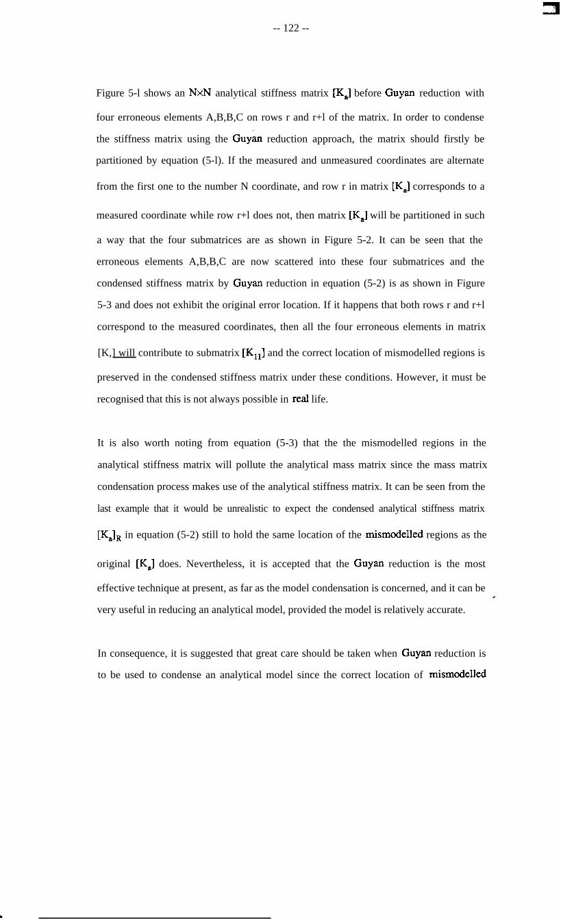
-- 122 --
Figure 5-l shows an NxN analytical stiffness matrix @,I before Guyan reduction with
four erroneous elements A,B,B,C on rows r and r+l of the matrix. In order to condense
the stiffness matrix using the Guyan reduction approach, the matrix should firstly be
partitioned by equation (5-l). If the measured and unmeasured coordinates are alternate
from the first one to the number N coordinate, and row r in matrix [K,] corresponds to a
measured coordinate while row r+l does not, then matrix &] will be partitioned in such
a way that the four submatrices are as shown in Figure 5-2. It can be seen that the
erroneous elements A,B,B,C are now scattered into these four submatrices and the
condensed stiffness matrix by Guyan reduction in equation (5-2) is as shown in Figure
5-3 and does not exhibit the original error location. If it happens that both rows r and r+l
correspond to the measured coordinates, then all the four erroneous elements in matrix
[K,] will contribute to submatrix [Krr] and the correct location of mismodelled regions is
preserved in the condensed stiffness matrix under these conditions. However, it must be
recognised that this is not always possible in real life.
It is also worth noting from equation (5-3) that the the mismodelled regions in the
analytical stiffness matrix will pollute the analytical mass matrix since the mass matrix
condensation process makes use of the analytical stiffness matrix. It can be seen from the
last example that it would be unrealistic to expect the condensed analytical stiffness matrix
[KJR in equation (5-2) still to hold the same location of the r&modelled regions as the
original [K,] does. Nevertheless, it is accepted that the Guyan reduction is the most
effective technique at present, as far as the model condensation is concerned, and it can bec
very useful in reducing an analytical model, provided the model is relatively accurate.
In consequence, it is suggested that great care should be taken when Guyan reduction is
to be used to condense an analytical model since the correct location of n-&modelled
.

-- 123 --
regions depends markedly on the coordinates experimentally identified and could possibly
be violated in practical cases when the number of these coordinates is necessarily
restricted.
S-4-2 Expansion of Measured Modes
Another strategy for coping with the incompatibility of the measured modes and the
analytical model is to expand the measured modes to the same coordinate set as the
analytical model, possibly using the analytical model itself. The possibility of scattering
the errors in the model is then avoided due to the fact that this process does not change the
connectivity in the original analytical model. It needs to be emphasised here that such a
mode expansion approach does not change the measured vibration modes at all: what the
approach does is to use the analytical model to interpolate those coordinates in the
experimental model which are not measured. Then, since the measured modes are
expanded by the analytical mass and stiffness matrices, it can be expected that modes
thus obtained are not exactly the same as those modes actually measured at all the
coordinates. In common with employing the Guyan reduction technique to condense the
analytical model to the coordinates tested, in the attempt to locate the the mismodelled
regions in the model which are to be pinpointed using those coordinates, location using
the expanded measured modes could only define the the mismodelled regions by those
coordinates tested and other coordinates in the expanded measured modes which were not
tested cannot be expected to be able to possess any error location information. This is
further explained below.
Suppose that coordinates i and i+l of a structure in Figure 5-4 are two among all of the
measured coordinates, while in the analytical model, ten coordinates are specified between
(and including) i and i+l and, further, among these ten coordinates, modelling errors
exist between coordinates j and j+l and there is no other modelling errors situated in other
part of the structure.

-- 124 --
If the model condensation procedure described above is used in order to apply methods
such as the EMM and the CMM, then the dynamic characteristics of the structure defined
by all the ten coordinates will be concentrated into coordinates i and i+l and, further,
coordinates i and i+l will also contain the dynamic characteristics information from all
other coordinates of the structure due to the condensation process specified by equations
(5-l), (5-2) and (5-3). It is hoped that an error location result will pinpoint the
r&modelled regions between coordinates i and i+l, provided the modelling errors
situated between these two coordinates (or more precisely, between coordinates j and j+l)
are not scattered into other part of the analytical model. Clearly, there is no point
whatsoever to expect any approach to locate the mismodelled regions between coordinates
j and j+l, because these two coordinates are not actually measured and the measured
mode shapes do not include them
If the measured modes are expanded using the analytical model, then the location
technique proposed in the early part of this thesis could be used to locate the mismodelled
regions and again, the mismodelled regions could only be defined between coordinates i
and i+l. However, in this case, there is no risk of the errors being scattered in the
analytical model and misleading the error location process.
5-S EXPANSION OF MEASURED COMPLEX MODES
In the previous studies, only the undamped case has been considered. The vibration
modes from measurement have been supposed to be effectively real so that they can be
expanded using the analytical model. As already mentioned, such applications have been
found in the literature, although not for the purpose of error location. However, some
vibrating structures are significantly damped and the vibration modes experimentally 0
identified will be complex. In order to use such measured modes to locate the
mismodelled regions in the analytical model and to locate the damping components from
the vibrating structure, the measured complex modes have to be expanded in some way to
the full coordinate set. Although there is no appropriate analytical damping matrix in
‘i

-- 125 --
existence, it is suggested that the measured complex modes could still be expanded in a
similar way as for the case of measured real modes, if some technical difficulties could be
solved.
A complex mode from measurement includes the natural frequency CO,, the damping loss
factor rl, and the complex mode shape (cp,). If the expanded complex mode shape is
denoted as { cp,] and which is:
(5-7)
where the first sub-mode (9,. } is the complex mode shape as identified experimentally
and the second sub-mode {Q) is the yet to be determined part of the complex mode
shape corresponding to the coordinates defined in the analytical model. Then, the usual
eigen-equations in equation (5-5) can be similarly partitioned into two parts, representing
respectively the coordinates in the complex mode shape (cp,r } experimentally identified
and those remaining to be specified from the analytical model, ((Q}):
(-(w:(l+~~~ [ LvI:; :;I+ [ :EL:: ~1) [zl;] = UN (5-ga,b)
The sub-mode ( qx2} of (cp,) can then be expanded by means of the analytical mass and
stiffness matrices:
~cp,,) = - { -w,2(1+Q)[h$21 + [&I 1“ { -o,2(l+rli)[&,l + lK2J Op,J) (5-9)
This mode expansion approach involves mathematically inverting a complex matrix and ’
this technical problem is discussed in Appendix 2. Thus, the measured complex modes
can then be expanded to the full coordinate set to be compatible with the analytical model,
based upon the analytical mass and stiffness matrices. Again, sorting the coordinates in
the expanded complex mode in equation (5-7) to the same order as the original analytical

-- 126 --
model will have to be done.
5-6 ASSESSMENT OF APPROACIIRS FOR COMPATIBILITY
The different approaches discussed and developed above to solve the problem of
incompatibility between the measured modes and the analytical vibration model of a
structure need to be fully assessed. It is thought that it would be appropriate to carry out
some specific numerical studies to assess these approaches. The system used in the
assessment is the 21 degree-of-freedom system in Figure 5-5. The analytical stiffness and
mass matrices can be constructed as the stiffness components and the masses are given
and hence all the simulated real analytical vibration modes are known.
It is supposed that the analytical model of the system has two ‘defects’, one being that the
stiffness component between coordinates 5 and 6 is underestimated by 20% and the other
being that there is a hysteretic damper in between coordinates 13 and 14. By considering
these two defects, the “experimental” model of the system can be constructed and thus,
the complex experimental vibration properties can be computed and are used to facilitate
this study. Table 5- 1 shows natural frequencies and damping loss factors of all 21 modes
for both models. The correct stiffness error matrix and the damping matrix of the system
is shown in Figure 5-6 and Figure 5-7 respectively.
If a modal test is conducted on the system using all the 21 coordinates, so that the
experimental vibration modes are defined in terms of the full coordinate set, then the
measured modes are completely compatible with the analytical model and there is no
requirement either to condense the model or to expand the modes. The measured complex
modes can then be used to locate the stiffness mismodelled region in matrix w,] and the *
damping elements in matrix [Hj. Figure 5-8 shows the location results of the approach
proposed in Chapter 4 using each of modes 1,2 or 3 respectively and it can be seen from
this figure that both the stiffness errors between coordinates 5 and 6 and the damper
.

-- 127 --
between coordinates 13 and 14 are well local&d.
In order to simulate the practical case where the experimental vibration modes are defined
at less coordinates then in the analytical model, the coordinates with odd numbers in the
complex experimental mode shape matrix are selected, representing the mode shapes
which are experimentally identified. Then, these modes are expanded by equation (S-9)
using the analytical stiffness and mass matrices. The thus-expanded modes are then used
to locate the stiffness mismodelled region in matrix [I<,] and the damping elements in
matrix [HJ.
Figure 5-9 shows the location results using the expanded modes 1, 2, 3, 5, 7 and 9
individually. Since the even-numbered coordinates in the expanded modes are expanded
by the analytical model, the stiffness errors and the damping will not be expected to show
up on these coordinates. Therefore, the mismodelled region in matrix [K,] will now be
defined between coordinates 5 and 7, both being experimentally-identified coordinates.
Indeed, the results using every expanded mode in Figure 5-9 indicate consistently the
stiffness errors between coordinates 5 and 7, with coordinate 6 showing no stiffness
modelling errors. The same argument for location of the damper between coordinates 13
and 14 is validated by Figure 5-9. The results using all the expanded modes in it
consistently locate the damping distribution between coordinates 13 and 15.
5-7 CONCLUSIONS
In practice, a degree of incompatibility always exists between the analytical model of a
vibrating structure and the vibration modes which are identified experimentally. If this c
incompatibility problem is not resolved, then no further use can be made of the measured
vibration modes to improve the analytical model.
Basically, there are two approaches to bridge this incompatibility: one seeks to condense
c

-- 128 --
the analytical model to those coordinates which are or can be identified experimentally and
the other attempts to expand the measured vibration modes using the existing analytical
model to the full set of coordinates.
No doubt, model condensation is a very economical means of studying the vibration
characteristics of a practical structure, considering the possible large numbers of
coordinates involved. As far as the location of the modelling errors and damping
components is concerned, however, it is believed that model condensation approach can
be quite vulnerable since the modelling errors in the analytical model will probably be
scattered during the condensation process and which will mislead the location effort.
In order to preserve the correct location of modelling errors in the analytical model, and
the correct damping distribution, it is suggested in this Chapter that the measured
vibration modes be expanded on the basis of the analytical model so that the expanded
modes can be used to locate the modelling errors and the damping distribution. A complex
mode expansion technique is also proposed.
Numerical assessment is carried out to validate the feasibility of the mode expansion
technique and results of using the expanded modes to locate the stiffness modelling errors
and the damping distribution simultaneously. It is suggested by the notable results that
such a mode expansion technique can be used in practical modal studies.
c ,

-- 129 --
21 DOFSystem
Analytical model Experimental model
Mode No.Undampedfrequency (Hz)
Dampedfrequency (Hz) damping loss factor
1i5
7”t
:7121314
::1718192021
10.247 10.43326.615 26.97448.950 48.99565.561 66.57477.270 78.51294.436 94.401
129.425 129.805154.283 156.197165.128 166.831184.810 184.808205.195 205.197221.929 221.932249.918 249.873269.443 279.794283.824 288.980290.790 290.928292.867 307.798330.097 330.097371.159 388.12347 1.907 47 1.907491.147 491.147
.040673
.079168BOO944.095412.038553XI05943.001260.006836XI03896.001321.000040BOO685.016287.000172BOO297BOO263.OOOOO1.OOOOOO
:ZZKZBOO153
Table 5- 1
Natural frequencies and damping loss factors of the 21 DOF system
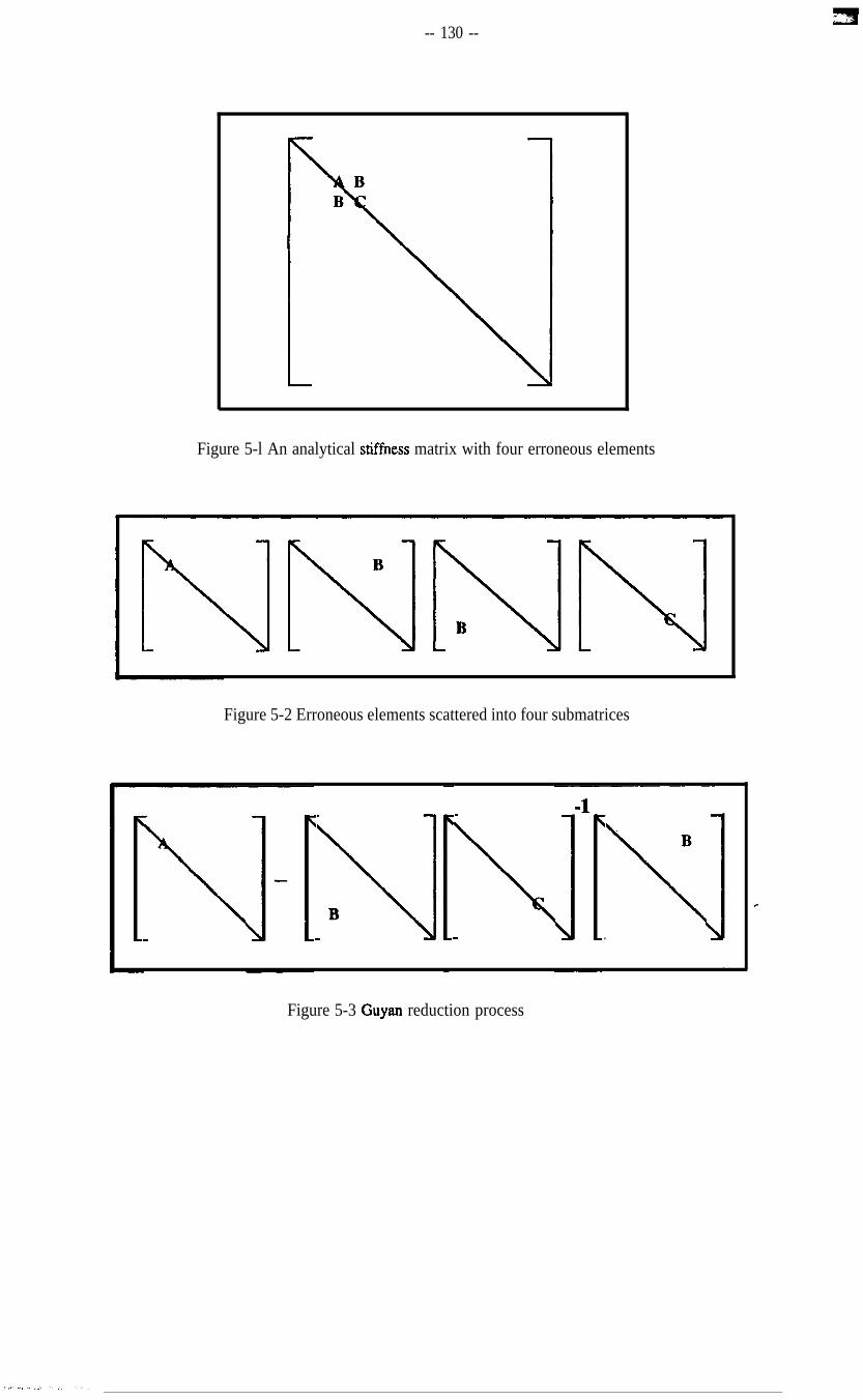
-- 130 --
Figure 5-l An analytical stiffness matrix with four erroneous elements
Figure 5-2 Erroneous elements scattered into four submatrices
_\\]
B_
.
\
B
\.
Figure 5-3 Guyan reduction process
c

-- 131 --
0 II 0 0 ?1 0
i j j+l i+l
Figure 5-4 A structure with coordinates ‘5” and “i+l” being tested
. . . . . . . . . . . . .
L,, L,,
. . . . . . . . . . . . .
Ll3 Ll4 Lx21
Figure 5-5 A 21 DOF system with an incorrectly predicted stiffness compomentand an unpredicted hysteretic damper
c
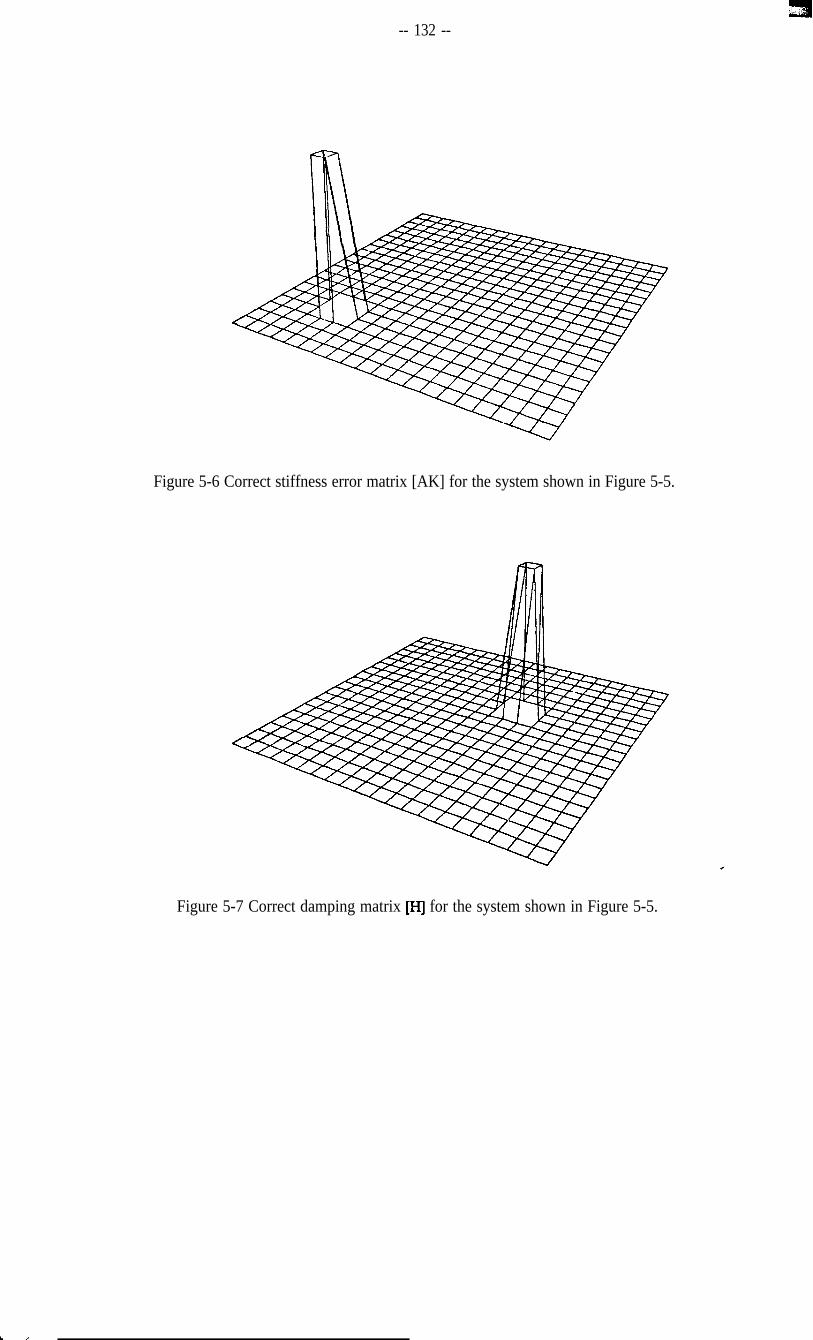
-- 132 --
Figure 5-6 Correct stiffness error matrix [AK] for the system shown in Figure 5-5.
Figure 5-7 Correct damping matrix [HJ for the system shown in Figure 5-5.
L ,

mode 1 only
mode 2 only
mode 3 only
Figure 5-8 Location of stiffness errors and damping elements in the system shownin Figure 5-5 using experimental modes 1,2 and 3 respectively.
Left-hand side column: location of stiffness errors.Bight-hand side column: location of damping elements.

Expanded mode 2 only
Expanded mode 3 only
Figure 5-9 Location of stiffness errors and damping elements in the system shownin Figure 5-5 using experimental modes 1,2 and 3 individually after theexperimental modes are expanded.
Left-hand side column: location of stiffness errors.fight-hand side column: location of damping elements.

c

-- 136 --
CHAPTER 6
APPLICATION OF MODELLING ERROR LOCATION
TO A PRACTICAL STRUCTURE
6-l INTRODUCI’ION
In the early parts of this thesis, it has been noted that the dynamic characteristics of a
structure are widely investigated by two approaches, these being theoretical modelling and
experimental testing. It has also been stressed that the dynamic characteristics can be fully
and correctly understood only if these two approaches are made in parallel, in order to
offset the weaknesses of both. The strong demand in vibration research and engineering
practice to use the measured vibration modes in order to improve the analytical model of a
vibration structure has also been identified.
Several methods which currently facilitate the model improvement process have been
reviewed and studied in Chapter 2. It is found that the main drawback of these methods is
that the resultant improved analytical stiffness or mass matrix does not adequately
represent the structure modelled analytically since these methods attempt to modify the
whole analytical model and end up with an ‘improved’ model which violates the actual
connectivity of the structure. The vibration characteristics deduced by a thus-improved
model will therefore not be correct and even the iteration process suggested in Chapter 2
cannot overcome this drawback and achieve the correct model. In addition, we lack an
appropriate method to investigate the damping properties of vibrating structures and the ’
proportional damping assumption is believed to be impractical in real Iife applications.
Since it is realized that, for most vibrating structures, the modehing errors inherent in their
analytical models are usually local - due to the sophisticated modelling techniques - and
L I

-- 137 --
these local errors in the models are referred to as the k&modelled’ regions, it then
becomes extremely important for the model improvement methods to be able to localize
these regions using a limited number of measured vibration modes. Without this location,
the models cannot be modified in the right areas and the model improvement can be
neither structurally meaningful and nor computationally efficient. A new approach has
been developed in Chapter 3 to enable the localisation of mismodelled regions using as
few as just one measured vibration mode. It has also been established that once the
mismodelled regions are localized, an iterative improvement of the analytical model can
become remarkably effkient. A similar philosophy has been applied to an investigation of
the damping properties and again, it is proposed that the major damping components of a
vibration structure can be located using a limited number of complex modes obtained by
modal testing and it then becomes promising to construct a meaningful damping matrix
for the analytical model by using the measured complex modes and the existing analytical
model, even if this contains some errors.
Although these approaches to localize the mismodelled regions from an analytical model
and the damping components of a vibration system have been successfully validated using
numerical case studies, it is necessary to investigate a real structure using the same
approach in order to demonstrate satisfactorily the feasibility of the applying the approach
in practice. This Chapter investigates the vibration characteristics of a beam structure
using both theoretical modelling and modal testing and analysis, in an attempt to
demonstrate that the local errors in the analytical model of the structure can be
successfully localized by applying the approach developed in this thesis.
6-2 ANALYTICAL MODELLING OF THE STRUCIUREc
The structure used in this study is the beam shown in Figure 6-1, with a uniform cross
section but with a joint, which is ignored in the predicted model. The structure actually
consists of two beam subsystems connected by a nut and bolt so that the tightness of the
joint can be adjusted to produce different local stiffness conditions. The beam is made of

-- 138 --
steel and is about 2m long with cross section of 25mm x 18Smrn.
A finite element analysis is carried out for this beam structure, ignoring the joint, so that
the structure is regarded as a uniform beam shown in Figure 6-2. This is divided into 9
equal length beam elements and, taking into account both the translational and the
rotational displacements in directions x and 8, as shown in Figure 6-3, mass and stiffness
matrices can be derived for the beam element (Appendix 3). Global analytical mass and
stiffness matrices which form the analytical model of the structure can then be
constructed. The analytical mass and stiffness matrices thus obtained have a dimension of
20x20. It is believed that the analytical mass matrix of this structure is reasonably accurate
since the structure does not have any sudden changes of section while the analytical
stiffness matrix obviously does not represent the true stiffness distribution because it does
not take account of the local stiffness change near the joint
The analytical vibration modes of the structure are obtained by the eigen-solution of the
analytical model. Table 6-l shows all the 20 natural frequencies of the analytical modes,
including two zero natural frequencies for the rigid body modes. The left hand column in
Table 6-2 shows the mode shape vectors of 4,5, and 6 analytical vibration modes derived
by the analytical model. It can be seen that the analytical vibration modes are defined in
both the rotational and translational coordinates and these are alternately positioned in the
mode shape vectors. Specifically, those odd-numbered coordinates are translational
coordinates and the even-numbered rotational ones.
6-3 MODAL TESTING AND ANALYSIS OF THE BEAM STRUCTURE AND THE 4
COMPARISON OF lTS MODAL MODEL AND FE MODEL
The modal testing was carried out with the structure supported by two soft strings at its
ends, simulating a free-free boundary condition, as shown in Figure 6-4. The testing was

-- 139 --
carried out at ten translational coordinates in the x direction, as indicated in the Figure 6-4.
As suggested by the modal testing theory, one column of the FRF matrix of a system is
theoretically sufficient to extract the modal model of the system, provided the excitation
point is selected such that all the interesting vibration modes can be excited. After careful
examination, it was decided that structure was to be excited at point 3 (coordinate 5)
where all the interested modes show up. Equipment set-up is also displayed in Figure
6-4. The frequency response analyser used in this test was Solartron 1250 analyser which
facilitates standard discrete sinusoidal signal. The Modal Testing software ‘POLAR’ is
used for the data acquisition and software ‘MODENT’ used for the analysis. Both
programs are developed in the Modal Testing Unit in this department and, in this study,
they were run on an HP computer.
A fast sinusoidal excitation sweep was used first in the frequency range of interest in
order to identify the vibration modes. Then, a roomed sinusoidal excitation was used in
the test and the acceleration response at each coordinate was recorded while the excitation
force is applied on point 3, so that the frequency response function (FRF) could be
obtained from the frequency response analyser. Figure 6-5 shows a typical frequency
response function obtained in measurement. Its counterpart in the Argand plane is shown
in Figure 6-6. The data exhibit quite clearly-defined modal properties for the structure
within the measured frequency range.
In this study, only three vibration modes were measured and analysed for the purpose of
stiffness error location. The measured natural frequencies of these three modes are shown
in the right hand column of Table 6-l. Table 6-2 compares these three measured vibration
modes with those predicted by the analytical model. The difference between the measured
natural frequencies and those predicted analytically, and that between the mode shapes, is *
apparent and is expected to be caused by the fact that the analytical model does not
correctly model the true stiffness distribution of the beam structure because of the joint.
Figure 6-7 shows the FRF data measured from point 6 within a certain frequency range
and the corresponding FRF data predicted by the FE model. It can be clearly seen that the

-- 140 --
vibration modes predicted theoretically exhibit different dynamic characteristics of the
structure from the vibration modes obtained experimentally. Again, this is due to the
different stiffness conditions which apply to the analytical and experimental configuration.
6-4 LOCATION OF THE MISMODELLED REGION IN ANALYTICAL
STIFFNESS MATRIX USING MEASURED VIBRATION MODE
641 Expansion of Measured Vibration Modes
In order to localize the modelling errors in the analytical stiffness matrix, the
incompatibility between the analytical model and the measured vibration modes in terms
of the coordinates specified has to be overcome first. As proposed in Chapter 5, the three
measured vibration modes are expanded to include those rotational coordinates which are
not measured, using the analytical mass and stiffness matrices. The three thus-expanded
measured mode shapes (rearranged to the original coordinate order as the analytical mode
shapes adopt) are listed in Table 6-2, together with the corresponding analytical mode
shapes for the sake of easy comparison. It can be seen fi-om Table 6-2 that the measured
translational coordinates in the expanded mode shapes are unchanged while the rotational
coordinates in the expanded mode shapes are effectively interpolated into the mode shapes
by the analytical model. In addition, the measured natural frequencies are not changed
during this mode shape expansion procedure.
6-4-2 Location of Mismodelled Region in the Analytical Stiffness Matrix
The three expanded measured vibration modes are then used to locate the errors in the
analytical stiffness matrix. Figure 6-8 shows the results of locating the errors using each *
expanded measured vibration modes individually and then using three measured modes
together, and this figure indicates that each result consistently points to the same region in
the analytical stiffness matrix where stiffness modelling errors exist. Namely, the errors
are confined in those elements between rows 13 and 17, corresponding to the testing

-- 141 --
points between 7 and 9.
To interpret the results shown in Figure 6-8, it has to be noted that the unpredicted joint in
the beam structure (ignored in the analysis) is situated between the test points 7 and 8 and,
according to the explanation of Chapter 5, the stiffness modelling errors should be located
between test points 7 and 8 (which correspond to the global coordinates between 13 and
16). However, the results in Figure 6-8 for using each expanded measured vibration
consistently indicate the stiffness modelling errors between testing points 7 and 9, which
relate to global coordinates 13 to 18. This is eventually answered by inspection of the
structure. Since the joint which is sited between test points 7 and 8 is close to point 9
side, the significant tightness of the joint eventually affects the stiffness condition between
points 8 and 9, so that the modelling errors are indicated not only between points 7 and 9,
but also between 8 and 9.
To be fully convinced of the location obtained above using the measured vibration modes,
one extreme condition is now considered. It is understood that the measured modal data
values could possibly vary due to the testing conditions, numerical calculation errors etc.
In order to simulate the possibility of different test results, and the consequence of that on
the location of the stiffness modelling errors in this study, all the measured natural
frequencies and mode shapes of the three modes are perturbed by five percent random
errors and these revised measured modes are then used, as before for the unperturbed
modes, to locate the errors in the analytical stiffness matrix. Figure 6-9 shows the results
using the revised modes 4, 5 and 6 individually and it can be seen that just the same
modelling error location is obtained, as before. This shows that the correct modelling
error location can be achieved even the measured data have some realistic errors.c
6-5 CONCLUSIONS
A practical application of the approach proposed in the early part of this thesis to locate the
r&modelled region in the analytical model of a structure has been carried out. The

-- 142 --
primary purpose of this part of the study is to assess the practical feasibility of the
approaches proposed so far in this thesis in locating the modelling errors which exist in
the analytical model of a structure using just a few number of the measured vibration
modes.
The structure upon which the investigation was performed is a beam structure with an
analytically ignored joint which causes the modelling errors in the analytical stiffness
matrix of the structure. The analytical model is obtained assuming the structure to be a
uniform beam and the analytical mass and stiffness matrices can be derived by Finite
Element modelling. The stiffness matrix thus derived contains errors relating to the local
area where the joint exists while the mass matrix is believed to be acceptably accurate
since there is no sudden mass change on the structure.
Modal testing was carried out using the ten translational coordinates of the structure only,
as the remaining rotational coordinates defined by the analytical model are technically
difficult to test. Only three vibration modes were identified experimentally.
Since an incompatibility exists between the measured vibration modes and the analytical
model, the three measured vibration modes were expanded using the analytical mass and
stiffness matrices, as suggested in Chapter 5. These three expanded vibration modes were
then used to locate the modelling errors assumed to be present in the analytical stiffness
matrix.
The results of using the expanded vibration modes individually to locate modelling errors
in the analytical stiffness matrix have consistently pinpointed the correct region in the
*matrix which relates the local area in the structure where the unpredicted joint is situated.

-- 143 --
Mode Natural frequencies(Hz) Natural frequencies (Hz)of complete model of measured modes
:
:
i7
;1011121314151617
:;20
E%Ei35097098.328 1 78.99
196.4980 170.16331.1097 287.83501.6208701.4584913.3696
1094.408 11598.56261811.25452076.28802398.38942824.39523430.90704355.47005758.28178079.045 18494.8225
Table 6- 1
predicted and measured natural frequencies of the beam structure
Sourse analytical model
Coords
measured mode expanded measured
:.34
:7
;10
::.1314151617
:;20
0.75065-3.0957 10.10554-2.82288-0.38516-1.51959-0.501000.49832-0.213221.954680.236801.903270.505820.373660.36850-1.60837-0.138172.86949-0.79146-3.12549
0.67238
0.15084
-0.28598
-0.46880
-0.3 1209
0.07480
0.44332
0.51650
-0.0725 1
-0.71877
0.67238-2.476150.15084-2.34668-0.28598-1.54197-0.468800.04462-0.312091.415240.074801.911410.443321.372090.51650
-1.31651-0.0725 1-3.25774-0.71877-2.89180
Table 6-2(a) Mode 4 - mode shapes from different sourses
* i’
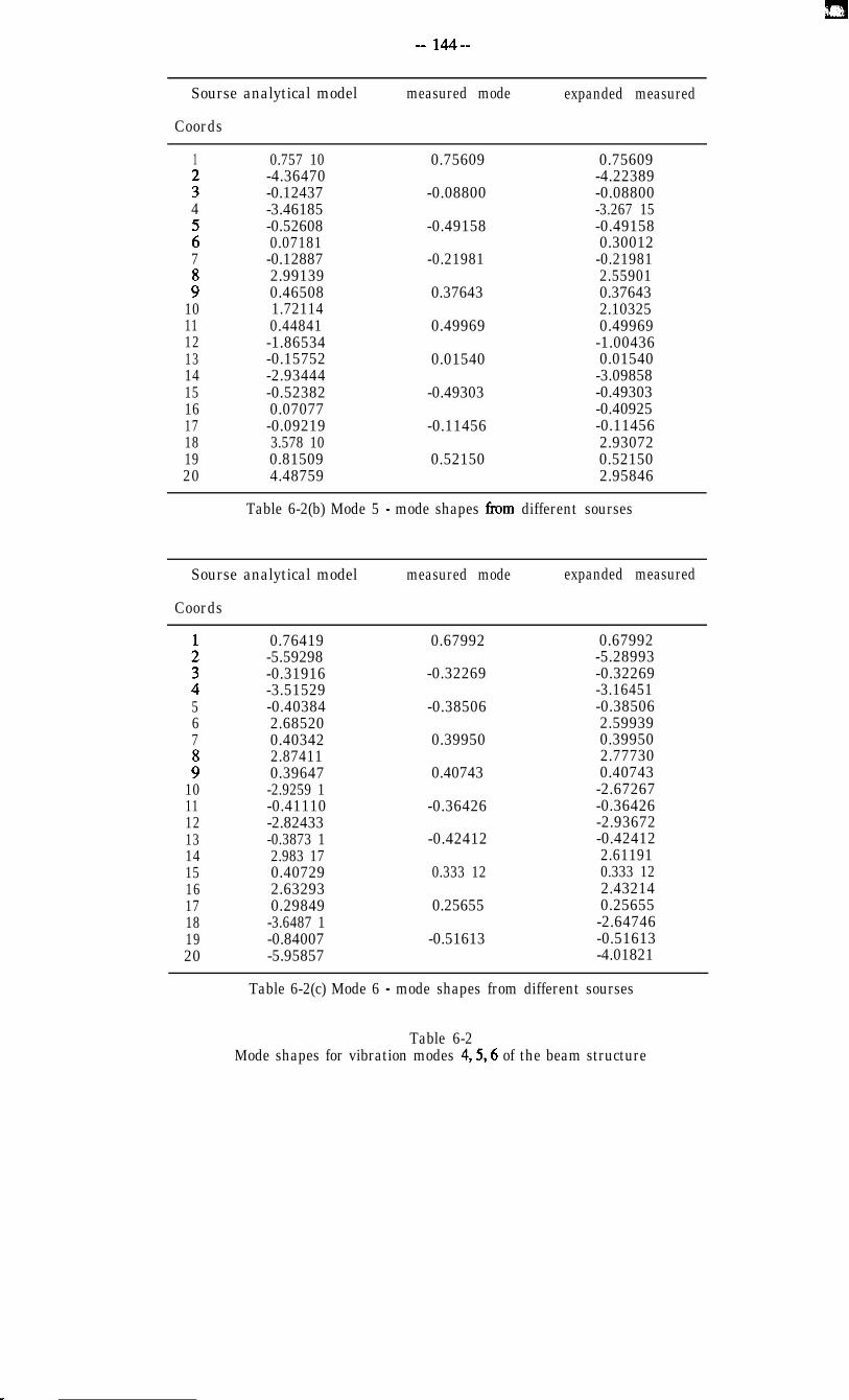
__ lM__
Sourse analytical model
Coords
measured mode expanded measured
1
i4
z7
:1011121314151617181920
0.757 10-4.36470-0.12437-3.46185-0.526080.07181-0.128872.991390.465081.721140.44841-1.86534-0.15752-2.93444-0.523820.07077-0.092193.578 100.815094.48759
0.75609
-0.08800
-0.49158
-0.21981
0.37643
0.49969
0.01540
-0.49303
-0.11456
0.52150
0.75609-4.22389-0.08800-3.267 15-0.491580.30012
-0.219812.559010.376432.103250.49969-1.004360.01540-3.09858-0.49303-0.40925-0.114562.930720.521502.95846
Table 6-2(b) Mode 5 - mode shapes from different sourses
Sourse analytical model
Coords
measured mode expanded measured
:.
:567
:1011121314151617181920
0.76419-5.59298-0.31916-3.51529-0.403842.685200.403422.874110.39647-2.9259 1-0.41110-2.82433-0.3873 12.983 170.407292.632930.29849-3.6487 1-0.84007-5.95857
0.67992
-0.32269
-0.38506
0.39950
0.40743
-0.36426
-0.42412
0.333 12
0.25655
-0.51613
0.67992-5.28993-0.32269-3.16451-0.385062.599390.399502.777300.40743-2.67267-0.36426-2.93672-0.424122.611910.333 122.432140.25655-2.64746-0.51613-4.01821
Table 6-2(c) Mode 6 - mode shapes from different sourses
Table 6-2Mode shapes for vibration modes 4,5,6 of the beam structure

I I I II I
Figure 6-l a uniform with an unpredicted joint

-- 146 --
Figure 6-2 FE modelling of a uniform beam
X X
I
Yb
Z
ä Y
Z
Figure 6-3 A typical beam element for FE analysis

Test point 1
Coord. No.( 1)
0 0 0 0 0 l 0
2 3 4 5 6 7 8 9 10
(3) (5) (7) (9) (11) (13) (15) (17) (19)
Beam structureA
Shaker 4
Charge amplifier
Power amplifier cl Sine signal geberator
Frequency response functionb
for modal analysis
Figure 6-4 Modal testing of the beam structure

-- 148 --
5 0
1 2 . 0 0 F r e q u e n c y H z . 6 9 8 . 0 0
Figure 6-5 A typical frequency response function obtained from modal testof the beam structure shown in Figure 6-4.
x
x x
X xX
XX _ _
XX
X
X
XXXX*cx x
X%
iit-- -7
X
x
XXXXX
,
fstrr-~
X
* x
* x
xxXX
,u2(N
REAL + ve.>
Figure 6-6 The FRF in Figure 6-5 is presented in the Argand plane.

-- 149 --
c
I ,

Expanded mode 4 only Expanded mode 5 only
Expanded mode 6 only A Expanded modes 4,5 and 6
Figure 6-8 Location of stifTncss enors for the beam structure shown in Figure 6-4using experimental modes 4.5 and 6 individually and then together
\ after the experimental modes arc expanded.
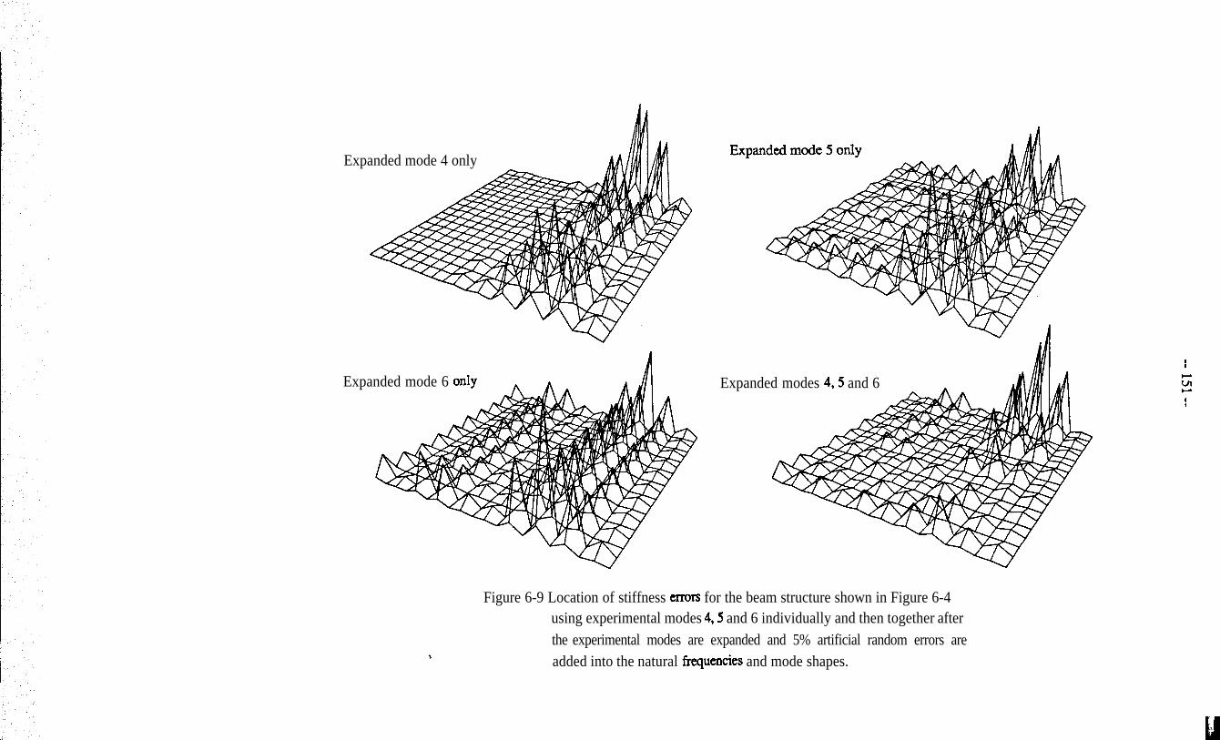
Expanded mode 4 only
Expanded mode 6 only Expanded modes 4,5 and 6
Figure 6-9 Location of stiffness errors for the beam structure shown in Figure 6-4using experimental modes 4,5 and 6 individually and then together afterthe experimental modes are expanded and 5% artificial random errors areadded into the natural frequencies and mode shapes.

c
-- 153 --
CHAPTER 7
MEASUREMENT OF NONLINEARITY
7-1INTRODUCFION
In the previous Chapters, we have covered one of the most important and demanding
topics in the recent vibration research: that of correlating the analytical model of a dynamic
structure and its measured vibration modes so that an improved model can be obtained.
This is expected to combine the advantages of the two widely used approaches (analytical
modelling and experimental testing) in order to understand better the dynamic
characteristics of the structure under investigation. The damping properties of a structure
have also been studied.
In those previous studies, it is assumed that linearity exists for the structures modelled
analytically and tested but it is realised that all real vibrating structures are nonlinear to
some degree. However, many of them may be nonlinear to a tolerable extent so that they
can still be investigated using the theory for linear structures. For those structures known
or suspected to be noticeably nonlinear in their vibration behaviour, the linear assumption
fails to be applicable and special analysis is needed to investigate the nonlinearity.
Generally, it can be said that nonlinearity is similar to the modelling errors and damping
properties discussed earlier in the sense that it also cannot be predicted analytically and
can only be identified by experimental measurement.c
The study of nonlinearity is very complicated. This results from the fact that the
superposition principles whereby the response of a system to different excitations can be
added linearly is not valid in the case of nonlinear systems. As a consequence, the
dynamic characteristics of nonlinear structures become excitation-dependent and much

-- 154 --
less predictable. Since the nonlinearity encountered in vibrating structures is often difficult
to identify, and even more difficult to quantify, they are in many practical cases significant
to the vibration behaviour of the structure, and the requirement for special investigation
methods is clear.
It is noted that theoretical methods have been developed extensively for those nonlinear
systems whose equations of motion can be expressed analytically. The fundamental point
of the analysis can be classified briefly as linearising either the parameters of a nonlinear
system or its vibration response. There are currently quite a number of methods which are
available to examine the vibration behaviour of a nonlinear system analytically. For
example, the Small Oscillation Method is an approach which replaces the nonlinear term
in the differential equations of a nonlinear system by its Taylor series with respect to
displacement and velocity and considers only the fast two terms, thereby extracting a
linear system which will exhibit a response like the nonlinear system; The Quasi-harmonic
Method[54] aims at deriving a periodic solution for a nonlinear system in the form of a
power series in E (a parameter which indicates the perturbations of the system and is
considered to be very small). Thus, a time-dependent solution which does not differ
appreciably from the solution of the corresponding linear equation can be sought. The
Method of Krylov and Bogolyubov supposes that the solution to the equation of a
nonlinear vibrating system is still in the same form as that of its linear counterpart, except
that the amplitude and phase are slightly varying with time and, as a consequence, the
approximate solution of the nonlinear system is a periodic function of both the amplitude
and phase angle, as weIl as time. An equivalent natural frequency and damping coefftcient
of the nonlinear system subjected to an external excitation can then be obtained as
functions of the response amplitudef 551. Iwan’s New Linearisation Method[561 is a
generalisation of the method of equivalent linearisation. It introduces a weighting function c
into the averaging integrals used in the equivalent linearisation method and suggests that a
nonlinear second order system can be replaced by a linear system in such a way that an
average of the difference between the two systems is minimized. It also shows that the
replacement is unique and can be accomplished in a straightforward manner.
. .
-- 155 --
Apart from the methods summarized above for general nonlinear cases, analysis could be
further developed to cope with systems having known types of nonlinearity. For instance,
such studies can be traced back to dates long before the computer was available[57] or,
they can be found from time to time in recent ~terature[~*l~[~~l.
Although many types of nonlinearity have been studied extensively, based on
mathematics and analysis used in control engineering, the theory is often not directly
applicable to experimental modal analysis of real structures because of the absence of
explicit equations of motion for practical vibration situations. The major difficulty in these
situations is the detection and identification of the nonlinearity when what is available is
the response of a nonlinear structure to excitation by external forces rather than an explicit
analytical description. Nevertheless, the theoretical study provides many specific and
frequently encountered types of nonlinearity with characteristic response patterns which,
in turn, provide a helpful reference in practical modal analysis.
7-2 EXCITATION TECHNIQUES
It is customary to assume that for linear structures, the dynamic characteristics will not
vary according to the choice of the excitation technique used to measure them. However,
the effects of most kinds of nonlinearity encountered in structural dynamics are generally
found to vary with the external excitation and hence the fust problem of a nonlinearity
investigation will necessarily be to decide a proper means of excitation so that the
nonlinearity can be easily exposed and then identified. There are currently mainly three
types of excitation method widely used in vibration study practice and each of them is
discussed below.c
7-2-l Sinusoidal Excitation
Sinusoidal excitation is the traditional excitation technique in vibration testing and also in

-- 156 --
recent modal testing practice. Although many other techniques such as random, transient,
periodic and pseudo-random excitations etc have been developed, sinusoidal excitation is
still commonly applied in practice because of its uniqueness and precision. The main
advantages of this excitation can be summarised as:
(a) sinusoidal excitation can accurately control the input signal level and hence it
enables a high input force to be fed into the structure. This is especially significant
when large structures are tested,
(b) for discrete sinusoidal excitation, the signal-tonoise ratio is generally good as the
energy is concentrated in one frequency band each time and even swept sinusoidal
excitation can normally achieve similar concentrated energy conditions compared
with other excitation methods;
(c) sinusoidal excitation is widely regarded as the best excitation technique for the
identification of nonlinearity in most applications of modal testing and analysis;
(d) when the harmonic distortion effects of nonlinearity are investigated, sinusoidal
excitation is also uniquely required.
It is the item (c) that contributes most to the continued wide application of this traditional
excitation technique. In this study, sinusoidal excitation is employed for each nonlinearity
simulated on an analogue computer in order to facilitate the nonlinearity identification
process.
The main drawback of the sinusoidal excitation technique is that it is relatively slow
compared with many of the other techniques used in practice. The obvious reason is that
the excitation is performed frequency by frequency and, at each step, time is needed for
the system to settle to its steady-state response. However, it is believed that for many
practices of the identification of structural dynamic characteristics, correct measurement *
results often become the primary criterion over time-saving in the test. For instance, when
the modal analysis results are to be used to improve an FE model of the tested structure -
an application which appears to be in great demand in recent years and has been
exhaustively discussed above - a major concern lies on the precision and comprehension

-- 157 --
of the modal analysis results. Consequently, sinusoidal excitaion is preferred in modal
testing in order to provide the post analysis stages with the optimum data.
7-22 Random Excitation
Random excitation attracts analysts and researchers primarily because of its potential time
saving in obtaining frequency response functions of the tested objects. Using this
technique, the system is excited simultaneously at every frequency within the range of
interest. This wide frequency band excitation enables the technique to be much faster than
sinusoidal excitation. Further, the effects of noise can be successfully eliminated by
averaging if the measurement time is long enough.
The derivation of the input and output relationship under random excitation relies on
Fourier transform theory and is based upon Duhamel’s Integral. As the Duhamel’s
Integral presumes a linear system behaviour, it has been suggested in the literature that the
linearity characteristic of the response from the random excitation is automatically
assumed. It will be shown below that this is not true. The actual reason for the inability of
random excitation to expose the nonlinearity from the response is the randomness of the
amplitude and phase of the input force.
In the measurement, spectral estimates for each recorded data block have random
amplitude and random phase. Thus, at each frequency the system can be considered to be
excited by different amplitudes and phases, sample after sample. By considering the effect
of nonlinearity as noise in the response, it can be understood that after the averaging
process the frequency response function obtained from the FFI’ analyser will always
comply with the behaviour of a linear system. It can then be roughly concluded that as far ’
as the identification of nonlinearity is concerned, conventional random excitation and
signal analysis is not a feasible technique in practice.
It should be noted here that the problem of impedance mismatch between the tested
_-

-- 158 --
structure and the shaker always exists and this can result in problem of noise. Usually,
the spectrum of the excitation signal is uniform along the frequency range of
measurement. However, when a mismatch occurs, the spectrum of the excitation force
applied to the structure may be distorted, yielding noise problems. The mismatch problem
is most serious at the resonances of the structure when the response spectrum at the
vicinity of resonance tends to drop because of the low impedance input to the structure,
resulting in a low signal-noise ratio.
Sometimes, when the dynamic modelling of a nonlinear system is of concern rather than
the identification of nonlinearity, the primary interest will be on extracting a linear model
of the system which behaves vibrationally in the frequency range of interest in as similar a
manner as possible to the nonlinear system, regardless what type of nonlinearity the
system possesses, then random excitation could be an effective technique.
7-23 Transient Excitation
Since the Fourier Transform was fust developed in the early nineteenth century, the
theoretical foundation had been provided for transient testing. However, not until digital
computers with FFT capabilities were developed did transient excitation and analysis
become practically feasible and has now received great interest because of the unique
characteristics differing from other excitation techniques.
In transient excitation measurement, the data involved are the time histories of the
excitation force f(t) and of the response x(t). The frequency response function is defined
by the division of the Fourier Transforms of these two time series signals. The
denominator is the Fourier Transform of f(t) whereas the numerator is the Fourier c
Transform of x(t):
H(o) = X(O) /F(W) (7-l)

-- 159 --
The actual computer analysis approach to obtain the frequency response function depends
on the estimates of the auto-spectrum of the force signal and the cross-spectrum of the
force and response. The computation is performed as:
H(o) = X(0) /F(O)
= X(o)F*(o) / F(o)F*(o)
(7-2)
where F*(o) is the complex conjugate of the Fourier Transform F(o) and SJo) is the
cross-spectrum of the force and the response of the system. Therefore, obtaining the
frequency response function in transient testing becomes a matter of spectral analysis.
The form of the forcing function in transient excitation is important. The input forcing
function theoretically suggested for transient excitation is of a pulse type. This is,
unfortunately, mechanically difficult to achieve in practice. Usually, a mechanical impact
is used to generate the required forcing signal. If the impact is well controlled, the forcing
signal would have a comparatively short time duration and contain desirable energy
spectral properties. However, a very short duration of an impact, covering a broad range
of energy distribution in the frequency domain, can be extremely difficult to obtain in
practice. This means that in the frequency domain the input force energy at high
frequencies is not always large enough to excite the system effectively. Hence, care
should be taken when transient excitation is applied to the case where vibration properties
at high frequency are of primary interest. Moreover, it is quite obvious that the excitation
frequency bandwidth cannot be controlled conveniently.
One possible alternative to the mechanical impact forcing signal is an electrical, instead of *
mechanical, impulse which can be applied to the strncture through a conventionally used
shaker. Indeed, this type of electrical pulse test has been adapted. Despite the fact that an
electrically-produced forcing signal has well controlled amplitude, a desired rectangular
c

__ 160 __
shaped pulse signal is still not easy to achieve due to a number of error sources such as
the “digitising error” occurring in the operation of A/D (analogue to digital) conversion.
Besides, the frequency characteristics of a shaker could be a problem and this is perhaps
more important,
Another forcing function referred to as “rapidly swept sinewave” or “chirp”, which is
classified in the transient excitation category, has been employed with success in recent
years[60]. Unlike the discrete sinewave used in sinusoidal excitation, the swept sinewave
here is of constant amplitude and has a sweeping frequency which varies rapidly and
continuously with time and has high cut-off rate at the starting and ending frequencies.
The time duration of the forcing signal can be as short as a few seconds. However, no
evidence has been found to back up the advantage of using such a excitation technique for
the purpose of identifying nonlinearity.
7-2-4 Comments on Different Excitation Techniques
Although there are a number of excitation techniques available nowadays for vibration
testing, the choice for the modal testing of a dynamic structure is by no means easy,
especially when nonlinearity is to be investigated.
Random excitation tends to excite the structure with a random force level and phase at
each frequency and thus the response data from a nonlinear system will behave as if the
system were linear, as the recorded data blocks are averaged. As the contribution of the
nonlinearity to the response differs from noise in that it is a systematic error and cannot be
averaged out, the response data from a nonlinear system will appear to be from a linear
system which is often referred to as a ‘linearised model’ of the nonlinear system, rather +
then the linear part of the nonlinear system. This is illustrated in Figure 7-l. Hence,
random excitation is not applicable for the purpose of the identification of nonlinearity. In
other cases, when the dynamic modelling of a nonlinear system is of interest, rather than
the identification of nonlinearity is sought, the primary concern will be on the extraction
L
-- 161 --
of a linear model of the system which will behave vibrationally in as similar a manner as
possible to the nonlinear system in the frequency range of interest, regardless of what
type of nonlinearity the system possesses, then random excitation could be an efficient
technique.
Transient excitation has noticeable
remarkably fast in performance. It
properties of convenience and simplicity and is
requires less instrumentation (for the case of a
mechanical impact test), facilitating mobile experiments. However, transient excitation
obviously attracts the same argument as random excitation in not being applicable for the
purpose of the detection and identification of nonlinearity. This is mainly because the
force level and phase of each data record is similarly not controllable as for the random
excitation case and, in addition, the frequency range is also difficult to control.
Nevertheless, low coherence often occurs at anti-resonances of the frequency response
function data when the impact test is carried out. This is mainly because of the low
signal/noise ratio at anti-resonances. This characteristic is different from the random test
where low coherence occurs both at resonances and at anti-resonances of the frequency
response function data. The reason for this difference is that for the random test, not only
can a low signal/noise ratio deteriorate coherence (which is similar to transient excitation
case), but also can the bias error do (also known as leakage problem)[701.
Sinusoidal excitation can have a well-controlled input force amplitude for each frequency
tested, and thus the nonlinearity inherent in the tested structure can then be exposed in the
response. In addition, it is most ideal to deduce harmonics when nonlinearity exists.
Therefore, this excitation technique is the most desirable one to use in the investigation of
nonlinearity. In this study, only sinusoidal excitation is applied.c
7-3 PRACTICAL CONSIDERATIONS OF NONLINEARWY MEASUREMENTS
As explained above, sinusoidal excitation is strongly favoured in measurement if
nonlinearity is expected and is to be studied. However, selecting sinusoidal excitation is

-- 162 --
merely the first step towards being able to identify the nonlinearity. There are still a
number of possible practical problems which need to be carefully considered, otherwise
the measurement will not be successful and, as a consequence, nonlinearity will not be
correctly identified.
The main difference between measurement of a linear structure and of a structure with
nonlinearity is that the excitation force level becomes significant for the latter case. In fact,
the force level becomes vitally important in determining the vibration characteristics of a
nonlinear structure. The effect of the excitation force level on the response of a nonlinear
structure depends not only upon the degree of the nonlinearity the structure possesses, but
also upon what type of nonlinearity it possesses. For many types of either nonlinear
stiffness or nonlinear damping, increasing the excitation force level will be similar to
enlarging the degree of nonlinearity as far as the response of the nonlinear structure is
concerned. Some other types of nonlinearity can be the other way around or even, the
excitation force level can be discontinuous (it will not affect the response until it reaches a
certain quantity). For instance, cubic stiffness provides a good example of enlarging the
degree of nonlinearity being the same as increasing the excitation force level while
Coulomb friction tends to affect the response less when the excitation force level
increases. Backlash stiffness is a nonlinearity where the excitation force level does not
affect the vibration response of a system possessing it until the force level is large enough
to make the response level to exceed a given limit.
As the vibration response of a nonlinear system is eventually related to the excitation force
level, careful consideration should be taken to select the force level for the measurement.
Thus, it would be appropriate to use a relatively large force level for a system with cubic
stiffness if the nonlinearity is to be detected and identified. However, great attention *
should be paid to the characteristics of the shaker which is normally used for vibration
measurement, since the shaker tends to distort the force level. In practice, the force level
will tend to decrease near resonances and this influences the effect of nonlinearity on the
frequency response function data. In order to expose the nonlinearity so that it can be

-- 163 --
identified, the following possible steps could be taken in measurement:
(a) using response control to build up a series of linearised models for the nonlinear
system. This method is extremely time-consuming and conventional linear
algorithms do not enable the extraction of the linear model of the system, i.e. the
damping loss factor and modal constant for the linear model of the system is not
obtainable unless very low or very high force conditions obtain, depending on the
type of nonlinearity.
(b) using a controlled force level to measure one frequency response function (FRF)
over the frequency range of interest or on the nonlinear mode. In this case, each
data point of this FRF comes, in fact, from one FRF of the former case, thus
containing the information of that FRF. Therefore, this type of measurement is
often applied in practice to study nonlinearity. The problem here is that to obtain a
controlled force level in measurement is by no means easy, especially when
nonlinearity is significant.
It will be seen later in Chapter 8 that nonlinearity investigation does not necessarily
require these conditional measurement above. In fact, it is possible to study nonlinearity
and to identify their types simply by using the data from conventional measurement where
no control is imposed at all.
74 SIMULATION FOR NON INVESTIGATION
7-4-l Significance of Simulation of Nonlinearity
For most practical nonlinear structures, the type and extent of the nonlinearity are 0
generally unknown and, further, the extent of the nonlinearity is not controllable for the
sake of nonlinearity analysis. The identification of nonlinearity will then be ineffective or
even unsuccessful unless the types of nonlinearity the structures often possess are
thoroughly studied beforehand so that their characteristics on the vibration behaviour are

well understood and categorised. It is believed that the most effective way to investigate
nonlinearity would be to simulate those types of nonlinearity frequently encountered in
practice and to thoroughly study their characteristics on the modal data so that those
categorised characteristics will then become useful references for the investigation of the
practical nonlinear structures.
The advantage of simulation analysis in nonlinearity investigation, besides the practical
necessity suggested above, lies mainly in the fact that a nonlinear system can easily be
simulated on a device such as an analogue computer by setting up the differential equation
which governs the simulated system and the parameters of the system can then be
conveniently adjusted to simulate different extents of nonlinearity. Hence, the response of
the simulated nonlinear system can be obtained and the vibration characteristics of the
nonlinear system can be thoroughly investigated which, in turn, will be referenced for the
nonlinearity investigation of practical structures.
7-4-2 Analogue Simulation of Nonlinearity
An analogue computer is a device whose component parts can be arranged to satisfy a
given set of equations, usually simultaneous ordinary differential equations. As for the
vibration study, the equations of motion to which a nonlinear system are subject are
usually second order ordinary differential equations, and so the analogue computer is an
appropriate device to be used. Figure 7-2 shows some of the basic elements used in this
study to construct the nonlinear systems. Because the analogue computer can only
integrate a function with respect to time (rather than differentiate it), a differential equation
has to be solved for the highest derivative in the equation.
In this study, several nonlinear SDOF systems, having either nonlinear stiffness or
nonlinear damping which are believed to be frequently encountered in practice, are
simulated on an analogue computer in order to investigate the dynamic behaviour of a
system having these types of nonlinearity.

-- 165 --
(1) A SDOF System with Hardening Cubic Stiffness
A SDOF system with hardening cubic stiffness and linear viscous damping is governed
by the following differential equation of motion:
% + 2r;c@ + coo2 (x+px3) = F(t) (7-3)
where 5 - viscous damping ratio of the system;
o0 - natural frequency of the system;
j3 - cubic stiffness coefficient;
F(t) - function of the excitation force.
In order to set up the analogue circuit for this system, equation (7-3) should be rearranged
into:
? = - ( -F(t) + 2@q,k + oo%+ coo2px3} (7-4)
In this study, the viscous damping ratio of the system is chosen as 0.005 and the natural
frequency as 10 rad/sec. The analogue circuit which simulates equation (7-4) is shown in
Figure 7-3.
(2) A SDOF System with Backlash Stiffness
A system with backlash stiffness and linear viscous damping can be shown in Figure 7-4
and the governing equation of motion is as follows:
% + 2&i + wo2x + q(x) = F(t) (7-5)
where:
i
+ %I% x>+x()
<p(x) = 0 -xc<x<+xc
- 661()~xo xc -x0
Here, parameter xc - which defines the linear response level of the system - is called the
. .

“response limit” and a linear system will have a infinite response limit. The other
parameter 6 which symbolises the stiffness change is referred to later as “stiffness ratio”
and a zero stiffness ratio will mean a linear system.
Again, in order to set up the analogue circuit for the system, equation (7-5) is rearranged
into:
;; = -{ -F(t) + 2504+ + CJ$X + q(x) ) (7-6)
With the same viscous damping ratio and the natural frequency as before, the analogue
circuit which simulate equation (7-6) is shown in Figure 7-5.
(3) A SDOF System with Piece-wise Stiffness
Piece-wise stiffness is a kind of nonlinear stiffness which is fairly often encountered in
practice. It differs from cubic stiffness in that its stiffness change is not continuous and
the stiffness effectively consists of a combination of several linear stiffnesses in different
response ranges. The backlash stiffness discussed immediately above is a type of
piece-wise stiffness. A system with piece-wise stiffness and viscous damping is governed
by the following general equation of motion:
j; + 250,~ + q(x) = F(t) (7-7)
where q(x) is a piece-wise function, contributing nonlinear stiffness effects and, for
instance, this function becomes as below for a bilinear stiffness:
Again, in order to set up the circuit for a system with piece-wise stiffness, equation (7-7)
is rearranged into:

-- 167 --
ii = -( -F(t) + 2&1.+,i + q(x) ) (74)
Figure 7-6 shows an analogue circuit which enables us to simulate various types of
piece-wise stiffness due to the positions of those switches indicated in this Figure. The
piece-wise stiffnesses this circuit enables us to simulate are shown in Table 7- 1.
(4) A SDOF System with Nonlinear Quadratic Damping
Nonlinear damping appears to be encountered less often than nonlinear stiffness in
practice, although this is actually not the case. This prejudice is partly due to the fact that
some dynamic structures are not significantly damped so that nonlinear damping may not
contribute as much as nonlinear stiffnesses and hence is not paid as much attention as
nonlinear stiffness. For fairly heavily damped structures, nonlinear damping is surely
another domain of nonlinearity which cannot be overlooked.
Quadratic damping is one of the many types of nonlinear damping encountered in practical
vibration problems. A SDOF system with linear stiffness and quadratic damping can be
described by the following equation of motion:
j;+aIxIx+o,Sr=F(t) (7-9)
where a is the quadratic damping coefficient.
Equation (7-9) can be rearranged to be suitable for the analogue set-up:
j;=_ (- F(t) + a I i I f + a+,%~) (7-10)
and the corresponding analogue circuit for this SDOF system having quadratic damping is c
shown in Figure 7-7.

-- 168 --
7-5 THE FREQUENCY RESPONSES OF THE NONLINEAR SYSTEMS
Once a nonlinear system is simulated on an analogue computer, a FRF measurement can
be performed as if it were a practical structure. As suggested earlier in this Chapter,
sinusoidal excitation is selected to provide the input (force) to the system and the
consequent acceleration (or velocity, displacement) of the system is regarded as that of the
structure due to the sinusoidal input force. The frequency response function (FRF) of the
nonlinear system can then be obtained from a frequency response analyser. The post
measurement modal analysis will then be based upon the FRF thus obtained.
However, the most important difference between measuring a simulated nonlinear system
and measuring a practical structure should be noted here. When sinusoidal excitation is
applied to measure a simulated nonlinear system without using a shaker, the force level
for the entire measurement will be constant (mainly controlled by the generator) as the
nonlinear property of a shaker which distorts the force level is not present. Therefore, the
nonlinearity could be readily exposed and its identification is relatively easy. However,
for the measurement of a practical structure, the force level will tend to vary near any
resonances which, in turn, influences the effect of the nonlinearity on the frequency
response function data.
Figure 7-8 shows the inertance-type frequency response functions obtained from a SDOF
analogue system measured using sinusoidal excitation and Figures 7-9 and 7-10 present
the corresponding real and imaginary parts plots. The system contains hardening cubic
stiffness with different cubic stiffness coefficients. Figure 7-11 shows the frequency
response functions of the same system with an unchanged cubic stiffness coefficient c
while the excitation force level varies and again, the corresponding real and imaginary
parts are shown in Figures 7-12 and 7-13. It can easily be seen from Figures 7-10 to 7-13
that increasing the cubic stiffness coefficient has an identical effect on the frequency
response function data of the system to increasing the excitation force level. Hence,

-- 169 --
although the extent of nonlinearity in practice is virtually impossible to change arbitrarily
as the simulated system can be, the effect of different extent of nonlinearity on the the
frequency response function of the nonlinear system can still be demonstrated by varying
the excitation force level so that the nonlinearity can be fully exposed and identified.
For a SDOF system with backlash stiffness, the frequency response function due to
sinusoidal excitation is influenced by the nonlinearity and the excitation force level in a
slightly different way to that seen for the cubic stiffness case. There exist three possible
conditions for this simulated SDOF system to vary and they are (a) the excitation force
level, (b) the response limit and (c) the stiffness ratio - both parameters having been
defined in equation (7-5). The frequency response of this system due to the change of
each condition is studied.
Figures 7- 14 to 7- 16 show the frequency response functions and their corresponding real
and imaginary parts obtained from a SDOF analogue system by using sinusoidal
excitation. The system containing hardening backlash stiffness has an unchanged stiffness
ratio and response limit as the excitation force level varies. The comparison of Figure
7-14 with Figure 7-11 will reveal the different effects of excitation force level on the
frequency response functions in these two cases, although they are all hardening-type
stiffness. For the cubic stiffness case, the frequency response function is affected
continuously by the excitation force level and this effect becomes greater as the excitation
frequency approaches the resonance frequency. However, the effect of increasing the
excitation force level for the backlash stiffness case does not show up unless the response
of the system exceeds a certain value, and this value is relevant to the excitation force
level itself. The difference discovered here could be a useful indication of distinguishing
between these two types of hardening stiffness. c
Figure 7-17 shows the frequency response functions of the same system containing
backlash stiffness with an unchanged stiffness ratio and a constant excitation level while
the response limit varies. It is evident by comparing Figure 7-17 with Figure 7-14 that

-- 170 --
the response limit varies. It is evident by comparing Figure 7-17 with Figure 7-14 that
decreasing the response limit of the system will have a similar effect on the frequency
response function to increasing the excitation force level. Figure 7-18 shows the
frequency response functions with an unchanged response limit and a constant excitation
level while the stiffness ratio of the system varies. It is interesting to note that the
consequence of different stiffness ratios does not show up until the response reaches a
certain level - which is believed to be the response limit of the system - and the frequency
response functions diverge more from the one without nonlinearity as the stiffness ratio
becomes bigger. For nonlinear damping cases, such a SDOF system also simulated on
analogue computer with quadratic damping, measurement can be carried out similarly
using sinusoidal excitation. Figure 7-19 shows the FRF data with different extent of
quadratic damping. It is evident that the natural frequency of the system changes little,
while the response is obviously governed by the damping extent.
As suggested above, the frequency response of a nonlinear system due to random
excitation will appear to be that of a linear system. This is because most types of
nonlinearity are excitation amplitude-dependent while the random force signal has
randomly varying force amplitude and phase angle. Therefore, the response of a nonlinear
system due to random excitation becomes an averaged result due to the different force
amplitude and as a consequence, the effect of the nonlinearity is linearised. To appreciate
this, random excitation is used in the measurement of the simulated nonlinear systems
discussed above. The measured frequency response function data eventually show
apparently linear behaviour for the nonlinear systems.
To understand fully the linearisation consequence of random excitation tests, questions
about the Fourier Transform algorithm have to be answered. As the Fourier Transform is c
a linear operation, suggestions of this algorithm linearising the nonlinearity could be
found in some literature[ 611. In this study, a special investigation was carried out:
sinusoidal excitation is used for the nonlinear systems while the frequency response
analysis is performed by an FFT analyser. It is found that as the excitation frequency

-- 171 --
sweeps, the frequency response function obtained by FFI’ exhibits exactly the same
results as shown in Figures 7-8 to 7-17 which are obtained from frequency response
analyser. This verifies the discussion in the earlier part of this Chapter - the Fourier
Transform is not responsible for the linearisation of the effect of nonlinearity in
measurement using random excitation. It is the randomness of the force amplitude and
phase angle of the input signal which linearise the response of a nonlinear system and
makes the system behave as a linear system
7-6 CONCLUSIONS
Nonlinearity is a widely-encountered phenomenon in practical dynamic structures. It is
sometimes neglected because of its small extent and little contribution to the vibration
response, but for many other cases, lack of proper means to deal with the nonlinearity
could be the primary reason for ignoring it.
Theoretically, the main difficulty introduced by the nonlinearity is that the superposition
principle whereby the response of a system to different excitations can be added linearly is
violated for nonlinear systems. As a consequence, the dynamic characteristics of
nonlinear structures become excitation-dependent and much less easily predicted.
It is believed that theory has been highly developed for those nonlinear systems whose
equations of motion are expressible analytically. There are currently quite a number of
methods which are available to examine the vibration behaviour of a known nonlinear
system.
However, since the nonlinearity inherent in vibrating structures is difficult to identify and c
even much more difficult to quantify, such theory is often not directly applicable to
experimental modal analysis because of the absence of explicit equations of motion. The
efforts of nonlinearity study in practical vibration analysis are then focussed on the
detection and the identification of nonlinearity in structures from measured FRF data

-- 172 --
Since the effects of most kinds of nonlinearity frequently encountered in structural
dynamics are characteristically variable due to the external excitation, the first problem of
the nonlinearity investigation will be to choose a proper excitation force so that the
nonlinearity could easily be exposed and then detected and identified. Amongst those
excitation methods currently widely used in vibration study, the sinusoidal excitation
method is strongly favored for nonlinearity investigation.
Analogue computer simulation is advantageous for nonlinearity investigations. This is
mainly because a nonlinear system can easily be simulated on an analogue computer and
the parameters of the system can then be conveniently adjusted to represent different
extent of nonlinearity. Hence, the response of the simulated nonlinear system can be
obtained and the vibration characteristics of the nonlinear system can then be thoroughly
investigated which, in turn, will be referenced for the nonlinearity investigation of the
practical structures.
SDOF systems with some frequently encountered types of nonlinearity are successfully
simulated on an analogue computer. Among those types of nonlinearity are cubic
stiffness, backlash stiffness, quadratic damping and various kinds of piece-wise stiffness.
Measurement using the sinusoidal excitation method can then be performed to obtain the
frequency response functions of these nonlinear systems. The refined modal analysis can
be carried out to detect and identify the nonlinearity by analysing these measured
frequency response function data and this will be extensively studied in the next Chapter.
c
., .I ..‘ ._. .,

Switch 1 A A B B A A A A
Stitch 2 z X Y Y Y X Y Y
coefficientmultiplier
kl0 O<kl<l m #O #0 ?4l &I 20
coefficientmultiplier
k2 =0 1 1 #1 1 1 fl #l
Backlashquantity
El=0 El=E2#0 El#E2tO El=E2#0 El=E2#0 El#E2?tO El#E2#0E2=maximum
Table 7- 1
Various types of piece-wise nonlinear stiffnesses

-- 174 --
Frequency response
b
FFT Frequency4 ,
A linearized model
,
Figure 7-l Linearisation effect of random excitation test

-- 175 --
x

-- 176 --
:X
40
--I
c
_,-.

-- 177 --
as
I I
sfe3a
0w
-I!--f
__!I!--7
0n
c

-- 178 --
40
:x
I
+
c

:X
+
hcL

-- 180 --
t
I
A
+c

-- 181 --
10 I I
is Hd
Figure 7-8 Inertance frequency response functions obtained from a SDOF system
with different extent of hardening cubic stiffness using sinusoidal
excitation.
I-
I-
I-
I-
I-
t-
I-
Lis 17
Figure 7-9 Real parts of the frequency
response functions shown in
Figure 7-8.
Figure 7-10 Imaginary parts of the frequency
response functions shown in
Figure 7-8.
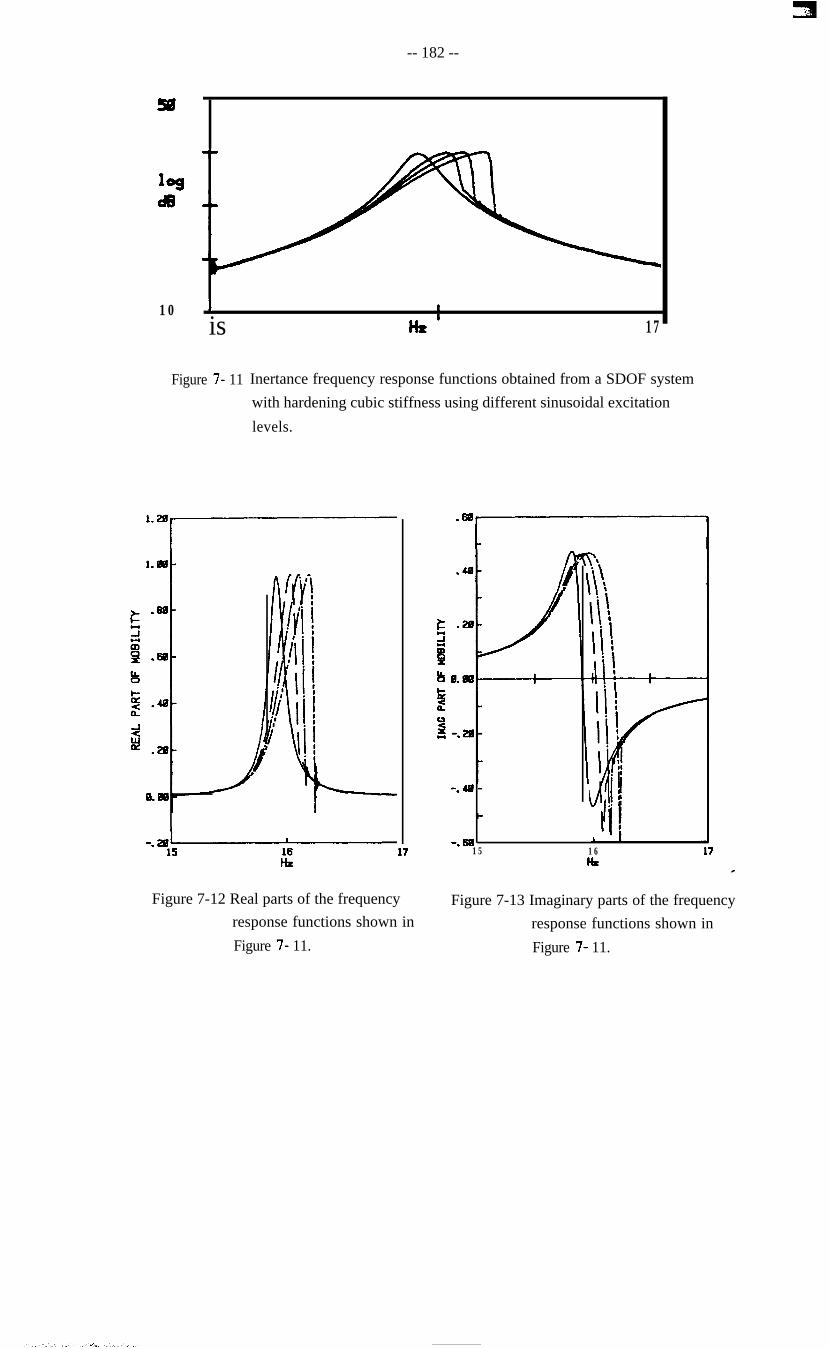
-- 182 --
10 1 I
is Hr‘ 17
Figure 7- 11 Inertance frequency response functions obtained from a SDOF system
with hardening cubic stiffness using different sinusoidal excitation
levels.
-.a‘115 IE
Figure 7-12 Real parts of the frequency
response functions shown in
Figure 7- 11.
-. 40 -
-. 6815 16 17
I4c
Figure 7-13 Imaginary parts of the frequency
response functions shown in
Figure 7- 11.

-- 183 --
J I
is H8’ 17
Figure 7-14 Inertance frequency response functions obtained from a SDOF system
with hardening backlash stiffness using different sinusoidal excitation
levels.
is
Figure 7-15
16 17
Real parts of the frequency
response functions shown in
Figure 7- 14.
.4&l-
~0.W~ I1
5su -.2m-
-. 4% -
Figure 7- 16 Imaginary parts of the frequency
response functions shown in
Figure 7- 14.
_

-- 184 --
logde
10 I I
is
Figure 7-17 Inertance frequency response functions obtained from a SDOF system
with different response limits of hardening backlash stiffness using
sinusoidal excitation.
10
Figure 7- 18 Inertance frequency response functions obtained from a SDOF system
with different stiffness ratio of hardening backlash stiffness using
sinusoidal excitation.
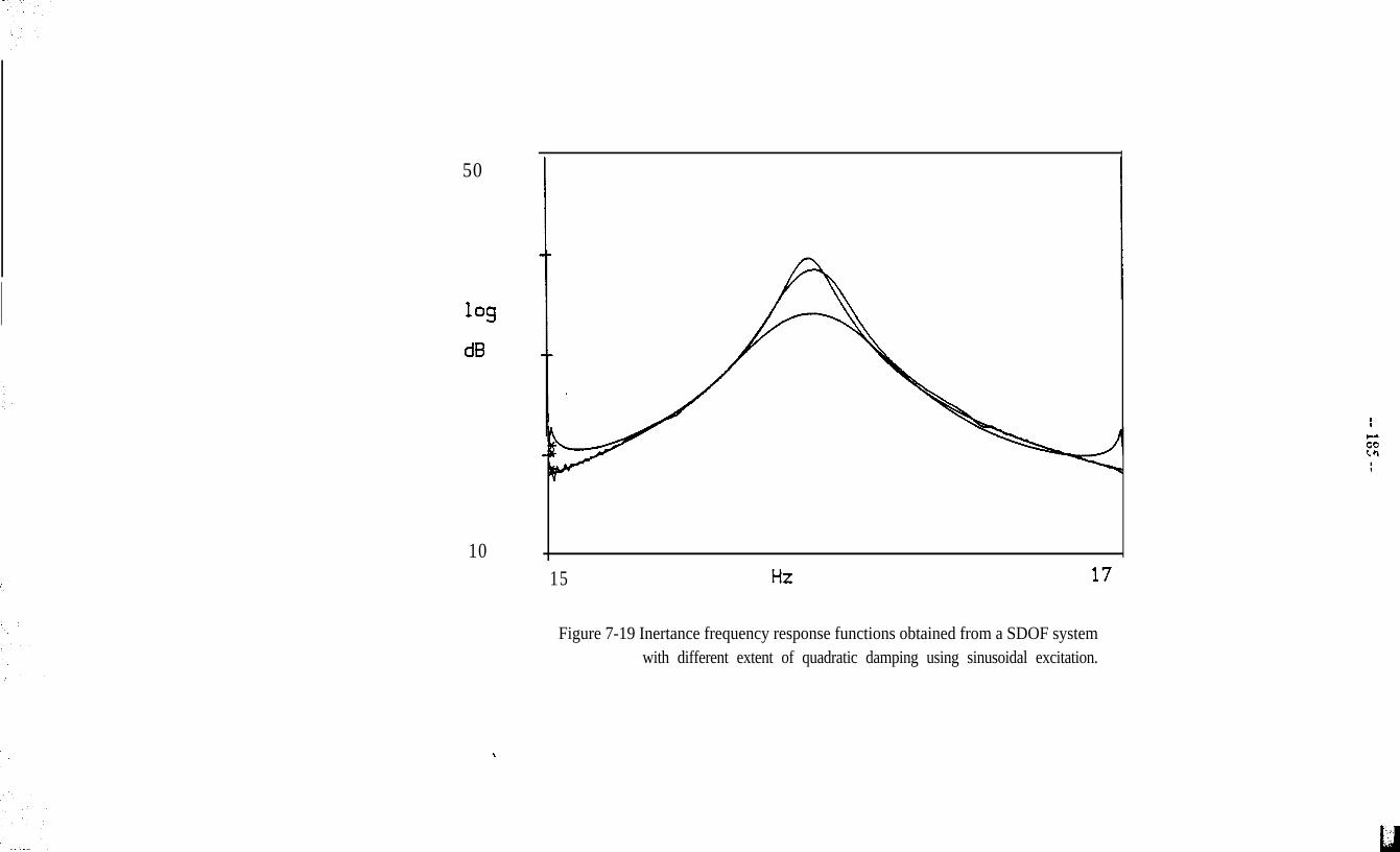
50
109
d6
1015 17
Figure 7-19 Inertance frequency response functions obtained from a SDOF systemwith different extent of quadratic damping using sinusoidal excitation.

c

-- 187 --
CHAPTER 8
MODAL ANALYSIS OF NONLINEAR SYSTEMS
8-l CURRENT METHODS AND APPLICATIONS OF MODAL ANALYSIS FOR
NONLINEAR SYSTEMS
Once it is suspected that a structure or a system is nonlinear, and measurement is carried
out as discussed extensively in the last Chapter, it is necessary to analyse the frequency
response function data taking account of the effect of possible nonlinearity. The
application of modal analysis methods to such FRF data depends upon the different
requirements on the nonlinearity investigation of the system. Generally speaking, there
are three possible requirements in practice for the results of modal analysis of a nonlinear
system. First, a linearised model may be required whose vibration response will be as
close as possible to the actual vibration response of the nonlinear system. Second, the
type of nonlinearity might need to be identified in order to enable the possible
establishment of a correct mathematical model of the nonlinearity and to seek the
possibility of predicting the vibration response of the nonlinear system to a wide range of
excitation conditions. Third, the identified type of nonlinearity is to be quantified in some
extent.
It is believed that the first requirement - to obtain a linearized model for a nonlinear system
without seeking the nature of the nonlinearity - is comparatively easy to achieve. In fact, a
family of frequency response functions with different random excitation force levels could *
always be measured, as suggested in the Chapter 7, and a conventional linear modal
analysis algorithm be employed to build up a series of models, each of them representing
the vibration behaviour of the nonlinear system under conditions of a certain excitation
force level. It is worth noting that such an investigation does not tell the nature and extent

-- 188 --
of the nonlinearity but, instead, it simplifies the nonlinearity problem by a piecewise
linearization approach.
However, practice is often confronted with the requirement of understanding the nature,
and even the extent, of the nonlinearity of a dynamic structure. Hence, current modal
analysis efforts are directed towards the detection of nonlinearity, and the identification of
the type and extent of nonlinearity in structures. To summarize, the following three
questions are to be answered by the appropriate application of modal analysis methods to
structures which might be nonlinear (Figure 8-l).
(1) Is the system or structure nonlinear?; (detection)
(2) If yes, what kind of nonlinearity does it exhibit?; and (identification)
(3) What is the extent of the nonlinearity? (quantification)
A large number of papers dealing with nonlinearity can be found in the literature in recent
years. As far as the detection and the identification of nonlinearity from the modal test data
is concerned, the methods commonly employed nowadays can be summarised below. It
is important to bear in mind that sinusoidal excitation is preferred in modal tests for all
these methods in order to let the nonlinearity be properly exposed rather than be averaged
out as happens in random excitation conditions. The advantages and disadvantages of
those methods currently used and summarised below will be discussed and the direction
of further developments will then be pointed out.
8-l-l Bode Plots
The basis of using Bode plots to detect the possible existence of nonlinearity, and to
identify it, is that the nonlinearity should systematically distort the frequency response c
function data and its real and imaginary parts from the form of the corresponding linear
system’s FRF data. As the linear system’s frequency response function is very well
recognized, the possible existence of nonlinearity could then be revealed by examining the
abnormal behaviour of the real and imaginary parts of the frequency response function

-- 189 --
data.
A typical example of nonlinearity being evident in the Bode plot is provided by the
frequency response function data shown in Figure 7- 11 and its corresponding real and
imaginary parts shown on Figures 7-12 and 7-13. The system from which these data are
derived has hardening cubic stiffness and it can be seen that this nonlinearity is clearly
exposed on the data. Similarly to this cubic stiffness case, the frequency response
function and its corresponding real and imaginary parts obtained from another SDOF
system, this time with backlash stiffness, are shown in Figures 7-14 to 7-16. Again, the
existence of the nonlinearity is apparent from the systematic distortion in the plots.
Although Bode plots of the frequency response function data can reveal the existence of
possible nonlinearity in most cases, it is after all merely a straightforward presentation and
no analysis of nonlinearity is involved, As a consequence of its simplicity, this method
usually cannot distinguish one type of nonlinearity from the other - e.g. the cubic stiffness
and backlash stiffness - when their effects on the frequency response function data are
fairly similar. Therefore, Bode plots can only be used to provide a rough and basic
examination of the existence of nonlinearity.
8-l-2 Reciprocal of Frequency Response Function
The Reciprocal of frequency response function data, which was previously discussed
briefly in Chapter 4, is offered as an alternative to modal analysis by the Nyquist circle fit.
It is based upon an assumption of SDOF behaviour. Basically, it is supposed that,
neglecting the residual effects of all other modes, the p mode of the frequency response
function (receptance) data of a structure will yield: c
oljl =Pjl
6$ co* + iTpr2
where: aj, is the receptance between test points j and 1;
(8-l)

-- 190 --
pjl is modal constant;
cer2 is the natural frequency;
TJ, is the damping loss factor.
Although the modal constant is in theory a complex quantity, it is often effectively real
and is treated thus here for this approach. The corresponding reciprocal of receptance &ta
is:
(l/ajJ =q- a2 + iqpr2
Pjl(8-2)
= Re(l/ajJ + h(l/ajJi
Perhaps the most significant advantage of using the reciprocal of receptance data is that
the mass and stiffness characteristics (natural frequency and modal constant in modal
data) and damping property (damping loss factor in modal data) are separated out into the
real and imaginary parts of the data respectively and hence, they can be dealt with
separately. In this case, the estimation of natural frequency and modal constant will be
considerably less affected by the damping loss factor than happens in the Nyquist
circle-fit or MDOF curve-fit, since this estimation is carried out only on the real part of the
reciprocal of receptance data, and which is physically quite reasonable. Similarly for the
estimation of damping loss factor, for the same reason. In addition, the extraction of
modal data from the reciprocal of the receptance data will not require the condition of
equal frequency spacing of the data which Nyquist circle-fit does.
The significant advantage of using the reciprocal of the receptance data becomes evident c
when modal analysis is made of FRF data from systems with nonlinearity. In these cases,
the effects of a nonlinear stiffness will show up on the real part of the reciprocal of
receptance data while the imaginary part of the data will be dominated by the effect of the
damping. Figure 8-2 shows the real and imaginary parts of the reciprocal of FRF data of

-- 191 --
a SDOF system with hardening cubic stiffness. It can be seen that the effect of the
nonlinear stiffness distorts the real part data noticeably but the imaginary part remains just
as for the linear case since the system here does not have any nonlinearity in the damping.
In Figure 8-3, similar real and imaginary parts of the reciprocal of FRF data for a SDOF
system with hardening backlash stiffness are presented. Again, the effect of the nonlinear
stiffness is clearly observed confined to the real part data.
This characteristic - that the effect of stiffness nonlinearity only shows up in the real part -
is in contrast with the standard FRF data format where the effect of any type of
nonlinearity will influence both its real and imaginary parts equally (e.g. the real and
imaginary parts of inertance FRF data). This is due to the fact that the real and imaginary
parts of the FRF data are related to each other and it will be seen in later discussion that
the Hilbert transformation makes use of this relationship between the real and imaginary
parts of the FRF data to investigate nonlinearity.
S-l-3 Modal Analysis and the Isometric Damping Plot
The isometric damping plot is one of the simpler methods available for the modal analysis
of nonlinear systems. Its application to the detection and identification of nonlinearity
relies on the argument that the nonlinearity will distort the spacing of the frequency
response function data along the Nyquist circle from their positions when no nonlinearity
exists. Its effect is unlike noise on the measurements, which also tends to distort the FRF
data, because the distortion provoked by nonlinearity is systematic rather than random.
Due to this character of systematic distortion, the damping estimates will vary according
to the specific point selection around the Nyquist circle and the nature of the distortion
displayed by the different damping estimates indicates the existence of nonlinearity. The -
following analysis seeks to explain the mechanism in detail.
It is well known that the damping loss factor for a vibration mode can be estimated by
curve-fitting the Nyquist circle (as shown in Figure 8-4) and using the following

-- 192 --
equation:
where o8 and ob are frequencies for two data points, one before and one after the
identified natural frequency. Also, it is known that for the FRF data from a linear system
without noise pollution, the damping estimate in equation (8-3) will theoretically be the
same no matter what pair of points on the Nyquist circle are chosen.
If the system is nonlinear, however, and the nonlinearity distorts the spacing of the FRF
data on the Nyquist circle systematically, as noted above, the then the damping estimates
from equation (8-3) will also vary systematically depending on the different points
selected, and variation in damping estimates becomes a good indication of the
nonlinearity. Figure 8-5 shows the Nyquist plot of the FRF data for a SDOF system with
hardening cubic stiffness and the corresponding isometric damping plot. It can be seen
that the nonlinear stiffness produces typical damping variation on the isometric damping
plot. In Figure 8-6, a similar Nyquist plot of the FRF data from a SDOF system with
hardening backlash stiffness and the isometric damping plot are shown. Again, the
damping variation in the isometric damping plot caused by the nonlinearity exhibits a
strong characteristic.
8-l-4 The Hilbert Transform
The Hilbert transform is a method for calculating the imaginary part of a complex
frequency response function from its real part (and vice versa), under certain conditions.
According to the Cauchey-Rieman theorem, a mathematically hatmonic complex analytical ’
function possesses the property that its real part can be derived from its imaginary part
and vice versa. This relationship is known as a Hilbert transform pair. In recent years, the
Hilbert transform technique has been borrowed from control engineering and applied to
vibration research for the identification and analysis of nonlinearity in structural
.I . ., , .‘..

-- 193 --
dynamics. In the following, the definition of the Hilbert transform will be briefly
reviewed and the basis for its application to modal analysis will be outlined, together with
several application examples.
S-141 The Principle of the Hilbert Transform
The Hilbert transform of a mathematical function f(x) is defined as an integral and is
denoted as H :00
F(x) = l/rt f(x’) dx’/(x’-x)J-00= HVOOI (8-4)
The integral F(x) is a linear functional of f(x) and it can be shown from the theory of
random vibration that the integral in equation (8-4) can be obtained by convolving the
mathematical function f(x) with (-7tx)-‘, namely,
F(x) = (-~/RX) f(x) (8-5)
or H [f(x)] = (-~/XX) f(x)
Since the Fourier transform of (- l/rrx) is i(S g n co), where s g n is a sign function and i is
imaginary unity, it can be said that the Hilbert transform is equivalent to a particular kind
of filtering in which the amplitude of the spectral components are left unchanged but their
phases are altered by 7r/2. Thus, the application of the Hilbert transformations twice in
succession will reverse the phase of all components and the results will be the negative of
the originals:z
f(x) = -(-l/xx) F(x) (8-6)
00
f(x) = -~/IF J_F(x’) dx’/(x’-x) (8-7)

-- 194 --
orf(x) = - H [WI
8-l-4-2 Basis of the Application of the Hilbert Transform to Modal Analysis
The frequency response function of a dynamic system G(o), which is a function of
frequency o, is the Fourier transform of I(t), the impulse response function of the system
which is a time varying functionWI:
G(o) = J I(t) dot dt-00 (8-8)
or G(o) = F [I(N
where F denotes the Fourier transformation in this work.
Since the impulse response I(t) from a linear system is real and causal (a system is causal
if, for any input, the response at any instant of time does not depend upon the future
input: a linear dynamic system should always be causal), it can always be split into even
and odd parts:
I(0 = w,,, + 1(0,&-j
= (I(t) + I(-t))/2 + (I(t) - I(-t))/2
and the even and odd parts can be linked together by the following equation:
(8-9)
wodd = W,, s 9 n (0
Since the Fourier transform of the sign function s g n (t) is:
F [sgn(t)] =-i/no (8-l 1)
the Fourier transformation of both sides in equation (8- 10) yields:
F [I(Ooddl = F [I(~),,1 F [s g NOI
= F [I(t),,1 (-i/n@
(8-10)
(8-12)

-- 195 --
It can be validated theoretically[74]1[75],[76] that, for a linear dynamic system, the real
part of the frequency response function G(o) is the Fourier transform of the even part of
the impulse response function I(t), and the imaginary part of G(o) is the Fourier
transform of the odd part of I(t), namely:
Re(GW) = F D(t>,,l
Im(G(W = F II(Oodd]
(8-13a)
(8-13b)
Thus, it can be shown as below that the imaginary part of the frequency response function
G(o) can be obtained from the Hilbert transform of its real counterpart (the same
argument holds for the other way around):
H [ReG(o)] = (4/x0) Re(G(o))
= F [ F-‘[(-i/m) ReG(o)]]
= F [b&t) W,,ll
= ImG(o)
Therefore, it is demonstrated by the above analysis that for a linear vibrating system, the
entire frequency response function can be constructed by knowledge of either its real or
its imaginary parts only or, in other words, either one of them determines completely the
vibration characteristics of the system. It should be borne in mind that although it is
suggested above that the impulse response is obtained from test, this is merely for the *
sake of simplicity to depict the theory. In practice, any kind of measurement technique
could be used and the inverse of Fourier transformation of the frequency response
function should always provide the impulse response of the system, provided this is

-- 196 --
linear and no noise pollution is involved.
If a system is nonlinear, then its impulse response from an impulse test is normally still
causal, provided the system is time-invariant as most structures in practice are. However,
the inverse Fourier transform of the frequency response function obtained from a
sinusoidal excitation, which is suggested in Chapter 7 as a favorable measurement
technique, would become noncausal due to the nonlinearity[74]~[75]. Thus, the result of
the Hilbert transform of the real part of the FRF data will not be the same as the imaginary
part of the FRF as it will be distorted by the nonlinearity, nor will the transform of the
imaginary part be the same as the real part, as illustrated in Figure 8-7.
To apply the Hilbert transform to the detection and identification of nonlinearity in
vibration studies, the frequency response function of a vibrating system from sinusoidal
test is used and the Hilbert transform of its real part can be calculated (as can its imaginary
part) and compared with its imaginary part. Any discrepancy between the Hilbert
transform of the real part of the FRF and its imaginary part will then indicate the existence
of nonlinearity, provided the computation of the Hilbert transform is accurate enough.
Once different types of nonlinearity can be simulated, studied and categorized by the
Hilbert transformation, the nonlinearity found in test data could by identified with a
reference to those categorized nonlinearity.
Figure 8-8 shows the real and imaginary parts of the FRF for a SDOF system with
hardening cubic stiffness and also the Hilbert transform of each. It can be seen that the
existence of the nonlinear stiffness results in a discrepancy between the original FRF and
the Hilbert transform counterparts. In Figure 8-9, a similar FRF of a SDOF system with
hardening backlash stiffness and the Hilbert transforms are shown. Again, the.
discrepancy caused by the nonlinearity is evident. These discrepancies could also be
examined in Nyquist plane.

S-2 COlMMENTS ON CURRENT METHODS FOR MODAL ANALYSIS OF
NONLINEARlTY
Amongst those methods currently used for the modal analysis of nonlinear systems and
outlined above, the methods based on the Bode plot and on the reciprocal of FRF data can
be categorized as types which aim at presenting the FRF data in such a way as to show up
the nonlinearity. It might be thought that when the FRF data are presented in some other
way, such as the inverse of the Nyquist circle (which is a straight line for linear cases),
the effect of an existing nonlinearity could also be expected. Therefore, it is believed that
these two methods are convenient for a straightforward inspection for the existence of
nonlinearity but this approach is not rigorous enough for a precise modal analysis of the
nonlinearity.
On the other hand, two other methods, namely the isometric damping plot and the Hilbert
transformation, tend to detect and to identify nonlinearity by investigating its effect on the
FRF data. Specifically, the isometric damping plot method demonstrates the spacing
distortion caused by the nonlinearity and the Hilbert transform examines the violation of
the functional properties of the frequency response function introduced by the
nonlinearity.
An overall and thorough examination of the application of these four methods - (i) Bode
plot, (ii) reciprocal of frequency response function, (iii) isometric damping plot, and (iv)
Hilbert transform - presented above shows that all of them are more or less feasible and
convenient for the detection of nonlinearity. In other words, the first question put forward
at the beginning of this Chapter can now be answered reasonably convincingly. c
However, not all the methods can be used to identify the nature of the nonlinearity once
its existence is confirmed. For instance, the method of reciprocal of FRF data can clearly
demonstrate the effect of nonlinear stiffness but cannot identify its actual type clearly. For
other more sophisticated methods such as the isometric damping plot, the identification of

-- 198 --
the type of nonlinearity becomes possible if those commonly encountered types of
nonlinearity are well categorized beforehand. However, a conclusive identification is
often difficult to achieve, considering the application on the hardening cubic stiffness case
and hardening backlash stiffness case. The same argument holds for the Hilbert
transformation technique. Moreover, it is clear that unless the type of nonlinearity is
identified confidently, its quantification is out of the question.
Apart from the immediate discussion on the identification of nonlinearity types, one
important aspect in the modal analysis of nonlinearity which these current methods are not
fully able to cope with is the need to obtain the correct modal data when the system is
nonlinear. For instance, the modal constant and damping loss factor for a system with
nonlinear stiffness should, in theory, be the same constants as if there is no nonlinear
stiffness. However, their accurate estimation is usually hindered when conventional
(linear) modal analysis algorithms are applied to extract modal data from nonlinear FRF
data.
Based upon the above study and discussion, it can be said that modal analysis of
nonlinearity requires further development so that it can more conclusively identify the type
of nonlinearity from FRF data and, based on this identification, the extent of the
nonlinearity can then be investigated, if required. In addition, the undistorted modal data
could be extracted from the nonlinear FRF data. In the following study, a new
interpretation of the effect of nonlinearity on FRF data is examined and used as the basis
for a new method to facilitate modal analysis of nonlinear structures.
8-3 A NEW INTERPRETATION OF THE EFFECT OF NONLINEARITYONFRF
DATA FROM THE MODAL ANALYSIS VIEWPOINT *
8-3-l Interpretation of FRF Data with Nonlinearity
With reference to vibration theory, it can easily be seen that some types of nonlinearity

-- 199 --
have been studied extensively. Using the experimental modal analysis methods discussed
above, more types of nonlinearity have been simulated and investigated. However, it is
believed that there are some aspects in applying modal analysis to identifying the types of
nonlinearity which need to be interpreted theoretically before further development of
practical nonlinearity analysis can progress. In the following, some new insights into the
modal analysis of nonlinear systems will be presented from a very fundamental point of
view and, for the sake of simplicity, these are illustrated using a SDOF system with
nonlinear stiffness. The discussion commences with the equation of motion of the system
with the spatial parameters such as mass and stiffness. It is customary that a SDOF
system with cubic stiffness will be described by the Duffing equation, as is often referred
to in textbooks:
(8- 14)
where m, k, p and c stand for the mass, linear stiffness, cubic stiffness and viscous
damping coefficients of the system respectively.
The stiffness characteristics and the frequency response function of the system subjected
to a sinusoidal excitation (f=Fe’Of) are shown in Figures 8-10 and 8-l 1 respectively. The
type of frequency response function (FRF) shown in Figure 8- 11 is often observed in
modal testing results but its interpretation from the viewpoint of modal analysis has not
been fully explored.
Considering a sinusoidal excitation, f(t)=FeiWt, equation (8-14) becomes:
m% + ck + k(1 - px2/k)x = Feiot
or m? + cx + k&x = Feiot
(8-15)
(8-16) *
Here, k(i) is a function of the harmonic amplitude f. The receptance of the system can
then be defined as:

__ 20(-j __
a(o) = l/(k(i) - o?rn + iac) (8-17)
The corresponding receptance for the same system without the nonlinear stiffness can be
denoted with a ‘0’ subscript as:
a,(o) = l/(k - o’rn + ioc) (8-18)
It can be said equivalently that the nonlinear system has different values of stiffness at
different response amplitudes. If a sinusoidal excitation with constant force (F=constant)
is applied in modal testing, then a receptance FRF of the form in Figure 8-l 1 will be
obtained for a SDOF system with softening cubic stiffness.
Since it is realised that the receptance in equation (8-17) has different values at different
response amplitudes for a given frequency, a response control technique could be
employed experimentally, as described in Chapter 7, in which each measurement is made
with the response amplitude being kept at a chosen level in order to linearise the vibration
behaviour. Figure 8-12 shows the measurement results of from SDOF system with
softening cubic stiffness in the vicinity of the resonance by using different response
amplitude controls. It can be seen that, as predicted by theory, each curve conforms to a
linear model, although the parameters of the model in each case vary according to the
selected response amplitudes. This, in fact, is one procedure for formulating a series of
linearized models for the system and thus to determine k(ic) versus %.
If we draw a horizontal line on Figure 8-12 to represent a specific value of receptance
amplitude (see Figure 8-13), then, for this particular value of the amplitude at the exciting
frequency ‘o’ denoted in Figure 8-13, we can take the cross point between the FRF curve c
and that horizontal line, both representing the conditions of the response amplitude which
must be satisfied simultaneously. For each point before resonance thus chosen, there is a
corresponding point (0”) after resonance lying on the same FFW curve. Linking all the

-- 201 --
points thus deduced produces a new FRF curve (Figure 8- 13) which is found to be of the
same form as that in Figure 8-l 1. In other words, the response of a system with nonlinear
stiffness can be constructed from the properties of a family of linear systems, each, in this
case, having the same mass and damping properties but different stiffness values. The
usually-observed FRF of this nonlinear system with constant excitation level (Figure
8-l 1) is effectively a combination of the results of all the linear systems, each point
relating to one of them.
Based on this observation, it can now be explained in a new way why nonlinearity cannot
be identified directly from a single FRF measurement made using random excitation
since, in this case, the force level at each excitation frequency varies, causing the response
level at this frequency to be an averaged value. The resultant FRF can therefore be shown
schematically in Figure 8-14. The curve, in fact, is between the linear FRF (without
nonlinearity) and the FRF curve of maximum response level.
8-3-2 Interpretation of the Reciprocal of Receptance Data with Nonlinearity
8-3-2-l Stiffness Nonlinearity
The reciprocal of receptance data has been previously discussed in Chapter 4 for the
identification of damping type and in an earlier part of this Chapter as a tool for the
investigation of nonlinearity. It has been found hitherto that this technique is not
applicable for the conclusive identification of nonlinearity type by simple and direct
implementation. However, an appropriate interpretation of the reciprocal of FRF data
from the modal analysis viewpoint, similar to that of the ‘standard’ FRF data discussed
above, will reveal the inherent nonlinearity effect on the reciprocal of receptance data in a
way which has not been published so far.
understanding of the results from modal
explained below.
In turn, this revelation will suggest a new c
analysis of systems with nonlinearity, as
It can be seen from Figure 4-l that the real part of the reciprocal of receptance for a linear

!!!!I-.-- 201 --
points thus deduced produces a new FRF curve (Figure 8- 13) which is found to be of the
same form as that in Figure 8-l 1. In other words, the response of a system with nonlinear
stiffness can be constructed from the properties of a family of linear systems, each, in this
case, having the same mass and damping properties but different stiffness values. The
usually-observed FRF of this nonlinear system with constant excitation level (Figure
8-l 1) is effectively a combination of the results of all the linear systems, each point
relating to one of them.
Based on this observation, it can now be explained in a new way why nonlinearity cannot
be identified directly from a single FRF measurement made using random excitation
since, in this case, the force level at each excitation frequency varies, causing the response
level at this frequency to be an averaged value. The resultant FRF can therefore be shown
schematically in Figure 8-14. The curve, in fact, is between the linear FRF (without
nonlinearity) and the FRF curve of maximum response level.
8-3-2 Interpretation of the Reciprocal of Receptance Data with Nonlinearity
8-3-2-l Stiffness Nonlinearity
The reciprocal of receptance data has been previously discussed in Chapter 4 for the
identification of damping type and in an earlier part of this Chapter as a tool for the
investigation of nonlinearity. It has been found hitherto that this technique is not
applicable for the conclusive identification of nonlinearity type by simple and direct
implementation. However, an appropriate interpretation of the reciprocal of FRF data
from the modal analysis viewpoint, similar to that of the ‘standard’ FRF data discussed
above, will reveal the inherent nonlinearity effect on the reciprocal of receptance data in a
way which has not been published so far. In turn, this revelation will suggest a new c
understanding of the results from modal analysis of systems with nonlinearity, as
explained below.
It can be seen from Figure 4-l that the real part of the reciprocal of receptance for a linear

-- 202 --
system (but with little noise) conforms a straight line when plotted against frequency
squared. From equation (8-17), it can also be seen that the reciprocal of the receptance of
a SDOF system with a stiffness nonlinearity, and its real and imaginary parts, can be
expressed as:
l/a(o) = k(2) - 02m + ioc (8-19)
Re(l/cc) = k(g) - 02m and Im(l/a) = i6.X
As suggested earlier, the most significant advantage of using the reciprocal of receptance
is the separation of the stiffness characteristics from the damping property into its real and
imaginary parts respectively, and so the interpretation of the reciprocal of the FRF data
due to nonlinear stiffness can then be concentrated on the real part of the data:
Re(l/a) = k(ji) - cn2m
= m ( oru2(%) - o2 ) (8-20)
Equation (8-20) suggests that away from the resonance, where k(k) is dependent
considerably less on the response amplitude, Re(l/a) will effectively be the same as
Re(llae) - the real part of the reciprocal receptance data of the corresponding linear
system deduced from equation (8- 18) - while in the vicinity of resonance, each data point
of Re(l/a) effectively represents a different stiffness value k(a) or natural frequency
w,2(%), because the amplitude of vibration (a) is likely to vary considerably from point to
point.
In common with the previous interpretation of the FRF data with nonlinearity, it can be *
seen here that if the measurement is made with a controlled response amplitude each time,
the Re( l/a) versus o2 plot will be of the same form as that for linear case (i.e. a straight
line), except that for each of such a condition of constant response amplitude, the
c /

-- 203 --
Re(l/a) data points will be subject to a different linear model with different natural
frequency, since the system will take different stiffness quantity for each condition.
Schematically, each time the Re(l/a) points will lie on one straight line which has a
different offset due to different natural frequency w02(%) (or different stiffness), as
shown in Figure 8-15. Since we presume the system has constant mass and damping
quantities (i.e. they do not change with the force level) for the nonlinear stiffness case, the
modal constant of the system should not, in theory, vary according to force level and
hence these straight lines are all parallel one to another. However, one measurement made
with a constant force level can include all the information contained in those parallel lines.
This is because each Re( l/a) data point in this case comes from one of those parallel lines
for response amplitude-controlled measurements and thus contains the necessary
information to define that line. Figure 8-16 shows the principle and is actually the
counterpart of Figure 8-13 which is for the receptance FRF case.
&3-2-2 Damping Nonlinearity
Similarly to the nonlinear stiffness case, the
imaginary part of the reciprocal of receptance
interpretation can be extended to the
data to observe the effect of nonlinear
damping. In this case, the equation of motion of the system with nonlinear damping can
be written as below for a sinusoidal forcing function:
m% + c(%)x + kx = Feiot (8-21)
where c(W) represents the nonlinear damping which is a function of the harmonic
amplitude jz, and parameters m and k are mass and stiffness of the system and are
supposed to be constant.
cBased on the same argument as for the nonlinear stiffness case, it is clear that the effect of
nonlinear damping is concentrated in the imaginary part of the reciprocal of receptance
data, which takes the simple form:
Im( l/a) = c(i)0 (8-22)
b
-- 204 --
It is customary that for linear viscous damping case, the imaginary part of the reciprocal
of Eceptance data (denoted here as Im(l/c@) versus frequency appears to obey a straight
line as the harmonic amplitude function c(g) in equation (8-22) is actually a constant. As
the damping becomes nonlinear, it can be seen from equation (8-22) that for each constant
response amplitude condition, the nonlinear damping will not vary and the system will be
subject to a linear damping model. The imaginary part of its reciprocal of receptance data
becomes a straight line, just like the linear damping case although this straight line has a
different slope from the one of Im(l&,) data representing linear damping case, as shown
in Figure 8-17. Nevertheless, one set of FRF data obtained with a measurement of
constant force level can include all the information of those non-parallel lines. This is
because each Im( l/a) data point in this case conforms to a certain harmonic amplitude and
should lie on one of those radial lines, this data point then fully contains the information
of that line. Figure 8-18 exhibits the composition of the Im(l/a) data from a measurement
of constant force level.
8-4 A NEW METHOD FOR THE MODAL ANALYSE OF NONLINEAR SYSTEMS
8-4-l Modal Analysis of Stiffness Nonlinearity
Having presented the above interpretation of nonlinearity effects on FRF data, it now
becomes possible to apply this to the modal analysis of nonlinear systems and to develop
a new technique which will be fundamentally different from the conventional methods for
the modal analysis of nonlinearity. As the fmt phase of the technique, the modal analysis
of stiffness nonlinearity is studied. Nonlinear damping will be discussed later. c
Before embarking on a detailed discussion, it is worth re-emphasizing that nonlinear
stiffness is a displacement amplitude-dependent property of a dynamic system and that the
natural frequency of the system is therefore amplitude-dependent, too. Also for the sake

-- 205 --
of simplicity, it is assumed that the system’s mass properties are constant in this case (i.e.
they do not change with excitation force level) and hence the modal constant of the system
with displacement amplitude-dependent stiffness should not, in theory, depend on force
level.
Since for a given type of nonlinear stiffness, the reciprocal of receptance data has been
thoroughly interpreted from Figure 8-16, it is believed now that by analysing the
reciprocal of receptance data in accordance with the knowledge of the above
interpretation, the type of nonlinear stiffness can be convincingly identified. In the
following, it is supposed at first that the linear modal constant of the nonlinear system ‘A’
(i.e. the modal constant obtained when assuming the nonlinearity is removed from the
system) is known - although this may be very difficult to achieve in practice - although it
will be found later that this precondition is not necessary.
S-4-l-l Description of Methodology
As stiffness nonlinearity is amplitude-dependent, it is supposed that a relationship of
response harmonic amplitude versus natural frequency (equivalent to stiffness, since the
systems’s mass property does not change) is necessary to identify the type of
nonlinearity. Further, it would be ideal to quantify the nonlinearity because, unlike other
methods such as the isometric damping plot or the Hilbert transform to extract certain
indications of nonlinearity, this relationship reveals the nonlinear stiffness feature directly
and explicitly. If it is supposed that the Re(l/a) data of a nonlinear system, such as the
curve shown in Figure 8-16, is available from measurements, then a set of parallel lines
using the linear modal constant as the slope can be drawn on the plot of Re(l/a) versus
frequency squared. The line through each FRF data point represents a linear&d model of
the nonlinear system which is valid at a certain response amplitude, as exhibited by Figure c
8-13. Since each data point relates to a specific response amplitude, a plot of response
harmonic amplitude versus natural frequency is then obtained and this, in turn, shows
explicitly the nonlinear stiffness characteristics of the system.

-- 206 --
8-4-1-2 Algorithm for Modal Analysis of Nonlinear Stiffness
The algorithm of the above procedure can be initiated from equation (8-20). Using the
modal data instead of the spatial parameters such as mass and stiffness, equation (8-20)
can be written in terms of modal constant (A) and harmonic amplitude (k) as:
Re(l/cc) = ( (I+,~(%) - o2 )/A (8-23)
The plot of data Re( l/a) against o2 is a straight line for data without nonlinearity and the
natural frequency w02 is thus a constant. However, in the case of nonlinear stiffness, the
amplitude-dependent natural frequency can be deduced from equation (8-23), yielding;
~e2(f) = A(Re(l/a)) + O2 (8-24)
Equation (8-24) consists only of FRF data and modal data and it demonstrates that, if the
correct modal constant A is available, the receptance amplitude-dependent natural
frequency can be obtained from the reciprocal of receptance data and this is equivalent to
obtaining the nonlinear stiffness against the receptance amplitude. It is necessary to
mention here that since the linear modal constant is relatively difficult to obtain by
conducting a conventional modal analysis procedure on nonlinear data, a new technique
will be introduced later in $8-4-3 to derive an accurate modal constant estimate.
The stiffness is a property related to response amplitude (rather than receptance
amplitude), and so it is necessary to convert the latter to the former once the natural
frequency against receptance amplitude is deduced from equation (8-24). If the force level
is constant throughout a measurement (which is ideal but impractical), then the difference ’
between the two amplitudes (response and receptance) would be merely a scale factor, as
will be seen later. However, considering the inevitable non-constant force levels in a
measurement of a nonlinear system, the response amplitude of each data point is
irregularly related to the force level and hence, cannot be obtained stra.ightfoNvardly from

-- 207 --
the receptance amplitude of that point. Fortunately, it is found that obtaining response
amplitude from receptance amplitude is feasible with knowledge of the force level
information because the receptance and the harmonic response under a sinusoidal
excitation have a simple relationship:
a(o) = Xeiot/Feiot (8-25)
and the harmonic amplitudes of the receptance, response and excitation force are therefore
related to one another as:
la(o)l =IX(w)l / IF( (8-26)
where a(o) and X(o) represent the receptance and response amplitude under the
excitation frequency o, and F(o) is the excitation force amplitude from the shaker.
Thus, the displacement amplitude can be deduced frequency by frequency from the
receptance amplitude and the force level:
IXI = Ia( IFI (8-27)
Equation (8-27) reveals the important feature that if the force level is recorded in the
measurement, then modal analysis of nonlinear stiffness can be conducted on the FRF
data measured without requiring any force or response level control. This means that
standard measurements can be made, thus saving a great deal of experimental effort.
Once the response amplitude is deduced by equation (g-27), together with the
amplitude-dependent natural frequency obtained from equation (g-24), the stiffness
characteristics can be derived explicitly and it becomes possible to identify the type of ’
nonlinear stiffness and, possibly, to quantify it.

-- 208 --
8-4-2 Modal Analysis of Damping Nontinearity
The modal analysis of a damping nonlinearity is based upon the previously developed
interpretation and is subjected to the similar methodology as that for stiffness nonlinearity.
In common with that case, nonlinear damping is an amplitude-dependent property of a
dynamic system. Therefore, unlike the linear system which has a constant damping loss
factor, the loss factor of a system with nonlinear damping will be amplitude-dependent.
For the sake of simplicity, it can be assumed that the system’s mass and stiffness
properties are constant when nonlinear damping is studied. The primary aim of modal
analysis of systems with a damping nonlinearity would be - like that of stiffness
nonlinearity - to identify conclusively the nonlinear damping type and to develop a model
(of damping against response amplitude) for the system.
The vibration motion of a system with a damping nonlinearity is described previously by
equation (8-21) and the effect of damping nonlinearity on FRF data is concentrated on the
imaginary part of the reciprocal of receptance, defined by equation (8-22). As Figure 8-18
shows, each Im(l/a) data point relates to a different linearized damping model of the
system and each data point represents a different damping loss factor due to different
response amplitude. Hence, when the FRF data of a system with damping nonlinearity
are measured, a series of straight lines can be drawn on the curve of Im(l/cx) against
frequency, each of which represents a linear damping model for a certain response
amplitude. Further, the damping loss factor corresponding to each data point can be
estimated from the straight line which passes through the point in question and represents
a linear damping model. Thus, a nonlinear damping model (of damping loss
response amplitude) can be deduced.
In order to implement the methodology of modal analysis of damping
equation (8-22) can be rewritten in terms of FRF and modal data, yielding:
factor against
nonlinearity,
I I

Im( l/a) = 2&)9p /A (8-28)
where c(g) is the response amplitude-dependent damping loss factor which becomes
constant if the damping is linear.
Once the linear natural frequency “au ” and modal constant “A” are obtained from either
the Nyquist circle-fit or the real part of the reciprocal of receptance data, the damping loss
factor for each data point (which corresponds to a different response amplitude, x)can be
evaluated by:
e(g) = Im(l/a) A / 2~0~0 (8-29)
In order to develop the relationship of response amplitude versus damping loss factor, the
response amplitude of each data point has to be estimated from the measured data in the
same way as was introduced for the stiffness nonlinearity case. Specifically, the response
amplitude can be derived from equation (8-27) and thus the damping property of the
nonlinear system (against the response amplitude) can be then be modelled and the
nonlinear damping type be identified.
.
S-4-3 The Extraction of an Accurate Modal Constant Estimate
It can be seen from the above study for the new method of modal analysis of nonlinearity,
that the accuracy of the modal constant estimate is very important. In fact, both equation
(8-24) for the analysis of stiffness nonlinearity and equation (8-29) for the analysis of
damping nonlinearity require an accurate modal constant estimate. However, an accurate ,
estimation of this parameter can be very difficult to achieve when the measured data are
from a nonlinear system Even for a linear system, the modal constant is often determined
after the natural frequency and damping loss factor estimation for the Nyquist circle-fit
algorithm and, hence, any inaccuracy in the latter two will directly influence the reliability

-- 210 --
of the former.
In order to reduce the influence of an error in the modal constant estimate for subsequent
analysis of nonlinearity, an accurate modal constant has to be obtained somehow. In the
following, the linear case is first examined to investigate the effect of an erroneous modal
constant estimate on the natural frequency estimation using the Re(lla) data and to
investigate a new method of obtaining an accurate modal constant estimate. Then, it will
be shown how the same technique can be introduced into the modal analysis of nonlinear
systems to adjust the modal constant estimate so as to achieve a satisfactory nonlinearity
analysis.
For a dynamic system with linear stiffness properties, the natural frequency can be
evaluated from any Re( l/a) data point using the following equation, provided the modal
constant estimate A is correct:
au2 = Re(l/a)A + cu2 (8-30)
The natural frequency thus estimated should theoretically be the same no matter which
data point is employed. Figure 8-19 shows the Re( l/a) data from a linear system and the
receptance amplitude against the natural frequency estimated by equation (8-30) using
each data point individually. Clearly, the same natural frequency is obtained from each
data point.
If the modal constant estimate is in error by an amount denoted by AA, then equation
(8-30) will become: c
or,2 = Re( l/a)A + w* + Re( l/a)AA (8-31)
Equation (8-31) shows that the error in the modal constant estimate will perturb the
natural frequency estimation process and produce a systematic discrepancy in the result.

-- 211 --
Only at the point when Re(l/a) is zero is the natural frequency estimated correctly.
Equation (8-31) also suggests that since the discrepancy in the natural frequency estimate
is systematic due to an error in the modal constant estimate, it should be possible to alter
the modal constant estimate with frequency so that when the systematical discrepancy
disappears, the correct estimate of modal constant has been achieved, and so has that of
the natural frequency. Figure 8-20 shows the results of natural frequency estimation by
equation (8-31) with different amounts of AA and it is clear that as AA becomes smaller,
the natural frequency estimation from each data point becomes closer to the correct
answer.
The technique proposed above to obtain simultaneously correct modal constant and
natural frequency estimates is a procedure which is independent of the damping and it can
be a useful alternative to the analysis of data wirhout nonlinearity so as to improve the
modal parameter extraction. For the modal analysis of damping nonlinearity, the correct
modal constant and natural frequency estimates are required in equation (8-29) and it is
also expected that they can be obtained in this way.
8-5 APPLICATIONS OF THE NEW METHOD FOR THE MODAL ANALYSIS OF
NONLINEARITY
The new method for the modal analysis of nonlinearity proposed above has been applied
to several systems with various types of nonlinear stiffness or damping in order to assess
fully the feasibility of the method. Most of the systems have a SDOF with either one type
of nonlinear stiffness or of nonlinear damping. In this study, both analytical and electrical
analogue data are used. In a second stage of the assessment, FRF data measured on a
practical structure are employed and the nonlinearity is investigated.c

-- 212 --
8-5-1 Analysis of Stiffness Nonlinearity
A SDOF system with different types of nonlinear stiffness has been simulated on an
analogue computer1 631 and studied using the traditional methods including the Hilbert
Transform and the isometric damping plot. Among these nonlinear systems, a SDOF
system with hardening cubic stiffness is typical and the data measured from it are
employed here for this study.
The inertance FRF data and the reciprocal of receptance data of the system have been
given previously in Figures 7-8 and 8-2 respectively. The isometric damping plot and the
Hilbert Transform of the FRF data with this cubic stiffness have also been presented
previously - in Figures 8-5 and 8-7 respectively. It can be seen that the existing
nonlinearity is strongly indicated by both the damping plot and the results of the Hilbert
Transformation. However, the type of nonlinearity is not conclusively identified since
other types of nonlinear stiffness - such as backlash stiffness - may well produce similar
indications and it could be extremely difficult to distinguish them from each other in either
of these two methods.
By using the new method of analysis, the system’s property of response amplitude versu.s
the natural frequency (equivalent to the stiffness) evaluated from each Re(l/a) data point
has been obtained as shown in Figure 8-21. Here it can be seen that the system has a
continuously changing type of stiffness property and hence the possibility of backlash
stiffness is eliminated and cubic stiffness is proposed. For a SDOF system with
hardening backlash stiffness, the reciprocal of receptance data has been shown earlier in 4Figure 8-3. It has been found that the isometric damping plot and the Hilbert Transform
results in this case could easily be misinterpreted as if the system has cubic stiffness.
However, by using the new method of modal analysis, the backlash type of stiffness
characteristics of the system can be shown as in Figure 8-22 which exhibits the true

-- 213 --
nonlinear stiffness type and is rather clearly distinguishable from the cubic stiffness
characteristic.
S-5-2 Analysis of Damping Nonlinearity
When the new method is applied to the study of damping nonlinearity, the results are as
encouraging as those for stiffness nonlinearity. The FRF data from a SDOF with different
extents of quadratic damping are shown in Figure 7-19 in the last chapter. The existence
of quadratic damping could be suspected from the typical apple-shape Nyquist plot
provided its extent is rather large and measurement force constant. However, the
isometric damping plot does not clearly indicate this nonlinearity.
On the other hand, the FRF data with quadratic damping can be analysed using the new
method proposed in this Chapter, with the results shown in Figure 8-23. The plot on the
right hand side is the imaginary part of the reciprocal of receptance and that on left hand
side is the analysis result. Figure 8-23 demonstrates that the damping loss factor of the
system varies linearly according to the response amplitude and this happens to coincide
with the characteristic of a quadratic damping model. Figure 8-24 shows the imaginary
part of the reciprocal of receptance of a SDOF system with a dry friction type of nonlinear
damping and the analysis result. Again, the extent of the nonlinear damping at different
response amplitude is clearly uncovered. Therefore, it can be seen that the new method of
modal analysis is quite useful in conclusively identifying the type of nonlinear damping as
well as identifying that of nonlinear stiffness.
8-S-3 Practical Applications of the New Method
c
In practical applications of techniques to study nonlinearity, it is believed that - with the
exception of the possible uncertainty of the exact type of nonlinearity - the primary
problem lies in the difficulty of applying constant force or constant response measurement
conditions, both being strictly required by conventional methods of nonlinearity analysis.

-- 214 --
If the force is not kept constant, then the nonlinearity cannot generally be fully exposed
and conventional methods cannot produce convincing results for analysis of nonlinearity.
Likewise, if the response is not well controlled, then a linearized model of a nonlinear
system cannot be obtained.
However, by using the new method, neither force control nor response control is required
in the measurement whereas the nonlinearity can still be analysed. In the following, a
typical example from measurements on the analogue computer is given first to simulate a
practical measurement where no force control is used and it will be seen that the
nonlinearity is successfully analysed. Second, a practical example from measuring a
vibrating structure known to exhibit nonlinear characteristics is then studied and the
nonlinearity investigated.
The FRF data shown in Figure 8-25 are obtained from the model of a SDOF system with
cubic stiffness added. The measurement is carried out in such a way that the force level
simulates the practical case; i.e. near resonance, the force applied to the system decreases
significantly due to the characteristics of the shaker. The actual force level recorded in the
measurement is presented in Figure 8-26. It is evident that the FRF data in Figure 8-25 do
not indicate the existence of nonlinearity as would be expected if the force level were kept
constant throughout the resonance frequency range. Moreover, neither the reciprocal of
receptance plot shown in Figure 8-27, nor the modal analysis results given by Figure
8-28, provides any significant indication of a cubic stiffness characteristic. All this is
attributed to the non-constant force level employed in measurement.
The same FRF data were then analysed using the new method proposed in this Chapter.
The system is known not to have any damping nonlinearity, and the analysis correctly *
indicates a linear damping model by the form of the imaginary plot of (l/a). However,
the nonlinear stiffness is clearly indicated by the relationship of natural frequency against
response amplitude exhibited in Figure 8-29. The continuous natural frequency change
with response amplitude coincides with the cubic stiffness model. Hence, it suggests that
-- 215 --
the new method does not necessarily require force control or response control to be
applied during measurements in order to achieve a successful nonlinearity analysis, both
being extremely difficult to achieve in practice.
A practical structure referred to as the “NASTRAN structure” was then investigated. The
structure was known to possess certain type(s) of stiffness nonlinearity[61] while the
exact nature of the nonlinearity is still unknown. In this study, a discrete sine sweep was
used to measure FRF data, covering the fiist mode of the structure, although neither the
force nor the response was controlled in measurement. Hence, the structure was
measured in just the same way as would be used if no considerations were taken of the
existence of nonlinearity. The inertance FRF data obtained and the force level generated
by the shaker are shown in Figures 8-30 and 8-31 respectively. It can be seen from these
figures that since the force level was not controlled, the FRF data does not show
indications of nonlinearity. The same conclusion is drawn from results of the modal
analysis presented in Figure 8-32 by circle-fitting a Nyquist plot of the FRF.
The new method was applied to the measured data and a nonlinear stiffness characteristic
was clearly revealed by the results shown in Figure 8-33. The stiffness change with
response amplitude suggests that the first vibration mode of the structure is subjected to a
softening backlash type of stiffness since the stiffness appears to be constant within a
certain response amplitude range, while beyond this range, the stiffness tends to decrease
as the response amplitude increases. By close observation of the structure, it can be
supposed that this could be due to the joints by which components of the structure are
connected. If the response amplitude is very small, then there is effectively no slip within
the joints but as the amplitude increases, the slip does occur, thereby reducing the
stiffness of the structure. c
8-6 CONCLUSIONS
Once nonlinearity is suspected in a structure, different strategies can be applied to deal

-- 216 --
with it, depending upon the different requirements. Despite the difficulty in extracting
correct modal data in the presence of nonlinearity, the main problems put forward by the
nonlinearity for modal analysis are: (1) Whether a dynamic system or structure is
nonlinear?; (2) If yes, what type of nonlinearity is it? and, possibly, (3) What is the extent
of the nonlinearity?
In coping with the reality of nonlinearity in structural dynamics, it is understood that there
are three common requirements for the modal analysis which can be summarized as: (1)
detecting the existence of nonlinearity and then linearising it without need for the
knowledge of its type; (2) identifying the type of the nonlinearity and (3) quantifying the
identified nonlinearity in order to devise a correct model for the nonlinear system for
subsequent analysis purposes, such as response prediction.
Four commonly-used methods for the modal analysis of nonlinearity have been reviewed
in detail in this Chapter. It is noted that both the Bode plot and the reciprocal of receptance
methods are merely different presentations of the FRF data intended to show up any
systematical distortion caused by existence of nonlinearity. They are very convenient in
the nonlinearity detection stage but not so applicable for the identification of nonlinearity
type or its quantification.
The isometric damping plot and the Hilbert Transform both seek more specific indications
of the different types of nonlinearity. Apart from the evident results these methods
provide in validating the existence of nonlinearity, conclusive identification of its type
relies on a lot of prior studies and categorization of different types of nonlinearity
commonly encountered in reality but, even then, some types of nonlinearity have similar
indications in the results of both methods and could mislead the identification. c
On considering the measurement of a practical structure, it is realized that to achieve a
satisfactory control on either the force or the response levels is often extremely difficult.
Nevertheless, the detection of nonlinearity and identification of its type performed by the

-- 217 --
above methods strictly requires the FRF data from measurement with a fairly constant
force level. Moreover, the modelling of the identified stiffness nonlinearity relies on a
number of measurements with different amount of response control. These requirements
impose significant demands on the measurement process(es) associated with nonlinearity
studies.
Based upon the SDOF assumption, a new interpretation of the effect of nonlinearity in the
FRF data, and subsequently in the reciprocal of receptance data, is made. It is made
essentially from the viewpoint of modal analysis rather than the theory deduced from
known differential equations. It is shown that since a dynamic system having a stiffness
nonlinearity will take a different stiffness value with each different response amplitude,
every FRF data point from a measurement with constant force actually relates to a specific
FRF data curve measured with a constant response and so, in effect, contains all the
information of the latter curve. Therefore, it is possible to use one FRF curve measured
with constant force to identify the type of nonlinearity and to model it. The same
interpretation is made for damping nonlinearity case.
Based on this interpretation, a new method is proposed to analyse the nonlinearity from
measured FRF data. In addition to deriving an indication of the nonlinearity, this method
aims at discovering the relationship between the vibration response amplitude and the
extent of the nonlinearity (such as stiffness or damping quantity) from the FRF data
measured using sinusoidal excitation. Since this method reveals directly the nonlinearity
characteristics as a function of response amplitude, it provides more conclusive
identification results and immediately suggests the reference for quantifying or modelling
the nonlinearity. It is also seen that the condition of constant force is not necessary when
measuring the FRF data for the subsequent modal analysis. In fact, satisfactory analysis *
can be carried out as long as the response amplitude varies sufficiently to expose the
nonlinearity. As a consequence, the new method also suggests a technique to extract
correct modal data in case of nonlinearity.

-- 218 --
In addition to requiring neither force nor response control in measurement, another major
advantage of the method developed here is its simplicity, both of application and
interpretation. By separating the stiffness and damping effects (into the real and imaginary
parts of the reciprocal of FRF), there is the immediate benefit of establishing the type of
element in which any nonlinearity exists. Then, it is possible to extract the nonlinear
characteristic by a simple modal analysis process without further complex analysis.
Although the method is predicated on the assumption of a SDOF model, and the extension
to truly MDOF systems is difficult, this difficulty is a feature shared by most (if not all)
studies of non-linearity in practical modal analysis applications. In view of the
impracticability of dealing with actual structural nonlinearity in any but an approximate
way, this new approach has distinct advantages in such applications.
.

-- 219 --
Modal analysis
Nonlinearity detectionNo
Yes v
Linearity confirmed
4v
Linear&d model
End
Nonlinearity identification
End
-iEnd
LNonlinearity ;yIMIation )
Figure 8-l The strategy of modal analysis of nonlinearity

R e a l P a r t
-- 220 --
R e c i p r o c a l o f R e c e p t a n c e .
I m a g i n a r y P a r t .
- -
0
1 5 . 3 3 1 6 . 9 9 1 5 . 3 3 1 6 . 9 9F r e q . A 2 F r e q . h 2
Figure 8-2 Real and imaginary parts of the reciprocal of FRF data from the SDOFsystem with hardening cubic stiffness
R e c i p r o c a l
R e a l P a r t
o f Recept ante.
I m a g i n a r y P a r t .
0
1 5 . 7 0 1 6 . 6 5F r e q . * 2
1 5 . 7 0 1 6 . 6 5 cF r e q . h 2
Figure 8-3 Real and imaginary parts of the reciprocal of FRF data from the SDOFsystem with hardening backlash stiffness

-- 221 --
Nyquist plane
I isometric damping plot
Figure 8-4 Isometric damping of a linear vibration mode

-- 222 --
EflL + ve.>
Figure 8-5 Modal analysis mults of the FRF with hardening cubic stiffness
.
H
Figure 8-6 Modal analysis results of the FFU? with hardening backlash stiffness

-- 223 --
I Impulse test
Impulse response
10)
CAUSAL signal
I Fourier transform
Other tests
l
Frequency response function
G(o) (= F [I(t)I)t
I I
I7
I
SystemLINEAR
1
System1NONLINEAR
F - jG(“)l = I(t)
and CAUSAL
H [ ~e~(o)l= b-G@)1.
H [ hnG(o)l = [ Wi@)] I
and NONCAUSAL I
I H [ awl f bG(@lI
I H [ImG(o)l # [ IWW-91
Figure 8-7 Basic idea of the Hilbert Transform
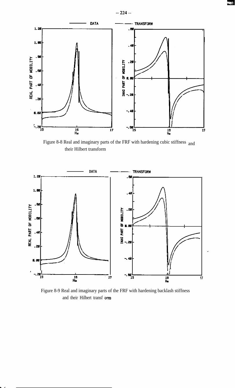
1
Figure 8-8 Real and imaginary parts of the FRF with hardening cubic stiffness
their Hilbert transform
DATA -.-. IRANSFDfW
’ -77Hz
and
Z -.20-
-.ti -
II
./---
f
/
/
Ii-.w’
15 2 17
Figure 8-9 Real and imaginary parts of the FRF with hardening backlash stiffness
and their Hilbert transf 6rm
c

-- 225 --
x
1 /
III \
w
\
\\\
c

-- 226 --
Hz
Figure 8- 11 Frequency response solution of the system subjected to a sinusoidal
excitation (f=Feiot), with stiffness characteristics shown in Figure 8-10
a(o) --
response level increases
Hz
Figure 8- 12 Receptance FRFs of a SDOF system with softening cubic stiffness in
the vicinity of the resonance using different response amplitude controls
.
c

-- 227 --
a(a) r----
.
Figure 8-13
1
0’ Hz co’ ’
Composition of the FRF with constant force from the FRFs withdifferent response amplitude controls using sinusoidal excitation
Figure 8-14 Illustration of the effect of random excitation on measured FRF
c

-- 228 --
Figure 8-15 Each Re(l/a) corresponds to a linear system model represented by one
straight line
Re( l/a:
Figure 8-16 Principle of using Re(l/a) data to analyse nonlinear stiffness
.
,

-- 229 --
linear model 1
coFigure 8-17 Each Im( l/cc) corresponds to a linear system model represented by one
straight line
L
_-L---_----
_----
0'
Figure 8- 18 Principle of using the imaginary part of the reciprocal of receptance data
to analyse nonlinear damping

-- 230 --
ReWar)
Figure 8-19 Re( l/a) data of a linear system and the receptance amplitude against the
natural frequencies estimated by equation (8-30)
Natural Frequencies
Figure 8-20 Effect of modal constant error AA on the natural frequency estimationusing equation (8-3 1)
.

-- 231 --
A n a l y s i s o f N o n l i n e a r S t i f f n e s s
R e a l P a r t o f l/R N a t u r a l F r e q u e n c i e s
1 5 . 7 0 1 6 . 6 5
F r e q . 62
.0010 .0050
Recept. Amp1 i t u d e
Figure 8-2 1 Re( l/a) data with hardening cubic stiffness and the analysis results
A n a l y s i s o f Non1 inear S t i f f n e s s
R e a l P a r t o f l/R N a t u r a l F r e q u e n c i e s
1 5 . 3 0 1 7 . 3 0
F r e q . ~2
all
.0005
Recep
.0045 *
t. Amp1 i t u d e
Figure 8-22 Re( l/a) data with hardening backlash stiffness and the analysis results

-- 232 --
Ana lys is o f Non1 inear D a m p i n gD a m p i n g C o e f f i c i e n t s I m a g P a r t of l/R
Y
ml
aah-u6
.0001 . 0002
Resp. Rmpl i tude
23 .67 27 .76
F r e q . ~2
Figure 8-23 Im( l/a) data with quadratic damping and the analysis results
Rna lys is o f Non1 inear D a m p i n gD a m p i n g C o e f f i c i e n t s I m a g P a r t o f l/R
--. -. 0013 . 0056
Resp. Amp1 i tude
_- --c
1 3 . 2 5 1 4 . 2 5
F r e q . ~2
Figure 8-24 Im(l/a) data with dry friction damping and the analysis results

-- 233 --
.l
.. .
. .. .
. .. .
. .. .. . ..
l .
015.00
Frequency Hr.16.99
Figure 8-25 FRJ? data obtained from a SDOF system with cubic stiffness
-217
-69CLb
iii
t:L
1I1
0
. . . . . . . . . . . . . . . . . . .
..
.
_- -_15 .88
Frequency Hr. 16.99
Figure 8-26 The force level used in the measurement
,

R e a l P a r t
__ 2-34 __
R e c i p r o c a l o f Recept ante.
I m a g i n a r y P a r t .
1 5 . 0 8 1 6 . 7 4Freq. h 2
-
0
_- __1 5 . 0 8 lb./4
F r e q . h 2
Figure 8-27 Reciprocal of receptance data of the FRF in Figure 8-25
SAL + ve.)
Figure 8-28 Modal analysis results of the FRF in Figure 8-25

-- 235 --
N a t u r a l F r e q u e n c i e s
.0001 .0005
R e s p . Amp1 i tude
Figure 8-29 The analysis results
. -
D a t a f r o m T O W VEIS c
4 0 . 0 0 4 9 . 5 9F r e q u e n c y H z .
Figure 8-30 Inertance FRF data measured from a practical structure
I ,

-- 236 --
. 1 0 9 r
0D a t a f r o m T O W V05
4 0 . 0 0F r e q u e n c y H z .
4 9 . 5 5 I
Figure 8-31 The force level generated by the shaker in the meaurement
EflL + ve. > aB
Figure 8-32 Modal analysis results of the FRF presented in Figure 8-30
,.

-- 237 --
N a t u r a l F r e q u e n c i e s
-----I--- - _____.
-
. 0004 . 0011
R e s p . Amp1 i tude
Figure 8-33 The analysis result using the new method

c
. .’

-- 239 --
CHAPTER 9
CONCLUSIONS AND SUGGESTION
FOR FURTHER STUDIES
9-l ANALYTICAL MODEL IMPROVEMENT USING MODAL TESTING
RESULTS
As current vibration practice demands more and more realistic mathematical models for
vibrating structures, the study of analytical model improvement using modal testing
results becomes increasingly important. This is because in the identification of dynamic
characteristics of practical structures, both the analytical prediction and the modal testing
have their own advantages and shortcomings. Using modal testing results to improve an
analytical model effectively makes use of the advantages of both while at the sarne time
overcoming their disadvantages and, it is by doing so that the most reliable mathematical
model can be achieved.
It is understood from numerical studies that the major pitfall for most methods currently
used, such as the constraint minimization method (CMM) or the error matrix method
(Em), to improve an analytical model using measured modes is to tackle it from a
purely mathematical viewpoint, such as an optimization one, rather than to consider the
structural characteristics as well, such as connectivity. As a consequence, the modified
model could often be optimal in a mathematically sense, but physically unrealistic. For c
instance, the modified analytical stiffness matrix could suggest a stiffness component
between coordinates i and j which are entirely unconnected on the real structure.
Repeatedly using these methods rarely shows a convergence to correct answers. This is
mainly because of the failure to preserve the physical connectivity and, furthermore,
L

-- 240 --
because of the attempt to ‘correct’ the correct parts in the analytical model in the model
improvement process.
Before and during this research for better methods of analytical model improvement, one
important concept is always borne in mind, i.e. what kind of model is a good model and
therefore is our target. It is believed that a good model is one which satisfies the following
conditions; (1) it represents correct physical connectivity; (2) the corresponding vibration
modes derived from it should agree with those observed in measurement and (3) it should
predict correctly those modes which we are unable to measure or which are not yet
measured. It is thought that condition (1) is a necessity for the model to be achieved - this
is actually ignored by many current efforts to improve an analytical model - and condition
(3) is the sufficiency for a good model. Philosophically, a successful model improvement
practice should aim at achieving a model which satisfies condition (3), by imposing
condition (2), based upon condition (1).
It is believed that the major errors will, in most cases, simply occur in a few localised
regions in the analytical model. The key issue for a model improvement study is thus to
be able to locate precisely where these major errors exist in the analytical model, using the
measured modes as input. This is because it provides a useful guide either for possible
further analytical modelling or for model improvement using measured vibration modes -
or both. As far as model improvement is concerned, the improvement can be directed
towards correcting those located errors in the model and the analytical model could thus
be improved much more realistically and effectively if these erroneous regions in the
model are somehow successfully located. In Chapter 3, a new method is proposed which
uses as few as just one measured vibration mode to locate the major errors in the
analytical model. Numerical case studies consistently suggest the correct error location *
achieved by this method In addition, a new iteration procedure - to apply current methods
such as the CMM or the EMM to improve an analytical model by correcting the located
errors in the model - is suggested for analytical model improvement. This new iteration
procedure has demonstrated marked advantages in achieving the correct model.

-- 241 --
Nevertheless, it should be stressed that the error location process does not confine itself
only for small error cases.
9-2 DAMPING PROPERTIES FOR PRACTICAL STRUCTURES
When the actual damping in a structure becomes significant and must be included in a
dynamic analysis, the conventional approach is often to assume proportional damping for
the analytical model. This assumption has been regarded as arbitrary since most practical
damping is not distributed in the same way as stiffness and/or mass. In fact, for many
practical structures, the major damping sources come from some restricted area(s), such
as the joints between components. Since the measured vibration data contain information
of the spatial damping distribution - although this information is neither complete nor
explicit - Chapter 4 describes an investigation of the damping properties by first locating
the major damping elements using the measured damped vibration modes. A more
accurate damping model can then be introduced based on the damping element location
results. It is also shown from numerical study that a correct damping matrix could be
obtained, even quantitatively, if an iteration with reference to the introduced damping
model is applied.
It is further understood that errors in an analytical model (error matrices [AM] and [AK])
and the damping matrix can all be regarded as a kind of local properties of a vibrating
structure - either local errors or local uncertainties. The best way of investigating such
local properties is perhaps to localise them first and then, to seek their possible
quantification. It has been found from this study that the mass and stiffness errors in an
analytical model, and the damping elements, can be localised using a relatively small
number of modes from modal testing results and these specified local properties can also c
be approximated or even correctly quantified.

-- 242 --
9-3 COMPATIBILITY OF ANALYTICAL MODEL AND MEASURED VIBRATION
MODES
A practical difficulty for some cases of model improvement is that the analytical model
and the measured vibration modes are incompatible in the sense of the coordinates
adopted. Usually, the analytical model uses a far greater number of coordinates than the
measured modes can to describe the vibration properties. For such cases, the methods
available for model improvement will not be directly applicable, unless this
incompatibility is resolved first.
There are basically two methods currently used to cope with this incompatibility and these
have been reviewed in Chapter 5, being: (1) to reduce the analytical model to the same
coordinates as the measured modes by Guyan (or similar) reduction methods and (2) to
expand the measured modes to the full set of coordinates as used by the analytical model
itself. It is found that, as far as the location of the errors in the analytical model is
concerned, method (2) is preferred because it preserves the physical connectivity of the
analytical model - and therefore the error location as well. Numerical study based on a 21
DOF system has shown that the errors existing in the analytical model can be correctly
located using the location technique developed in Chapter 3, after the ‘measured modes’
are expanded.
Since these two methods assume both the analytical and the experimental data to be real,
they are not applicable to study the damping properties and to improve the analytical
model when a structure is sufficiently damped that the measured vibration modes become
complex. However, a new method has been proposed in this thesis to expand the damped l
measured modes to full coordinates using the analytical model including only mass and
stiffness matrices. Thus, these expanded complex measured modes can be used, in a
similar way to the expanded real modes, to locate the damping elements and, at the same
time, to locate errors in the analytical mass and stiffness matrices.

-- 243 --
The location of errors in an analytical model using measured vibration modes has been
demonstrated by a practical application. The object used is a beam structure with two
straight beams jointed together by nut and bolt. It is supposed that this joint is unknown
so that the FE analysis predicts the stiffness properties of the structure as a continuous
beam, while the mass properties are the same with or without the joint. Although the
analysis covers the vibration characteristics of the structure in the frequency range up to
some 3000 Hz, only three vibration modes are actually measured, and only half the
coordinates are included. These measured modes are firstly expanded using the FE model
and are then used, individually and collectively, to locate the errors in the analytical
stiffness matrix. The location process successfully indicate the major errors
corresponding to the joint in the structure.
9-4 NONLINEARITY IN MODAL TESTING
All the previous studies assume the vibration of the structure or system investigated to
behave in a linear way, or that the nonlinearity could be ignored due to its small extent.
This assumption can be too optimistic for some cases where nonlinearity becomes
significant in the vibration characteristics.
Unlike theoretical studies, where the vibration characteristics of nonlinear systems can be
described by differential equations, the major problem in the realm of modal testing of
nonlinear systems is to study unknown types of nonlinearity. The key issue therefore
becomes identifying the types of nonlinearity, after their existence is detected. The review
and discussion of those methods currently used to investigate nonlinearity - all aiming
basically to identify nonlinearity from their effects on the measured data - have suggested +
their practical applicability. However, conclusive identification of the types of nonlinearity
is still problematic, because some types of nonlinearity can well produce quite similar
effects on the measured data.
__ 244 __
With the help of closer examination of the vibration data on nonlinear systems measured
using stepped-sine excitation, a new interpretation is proposed to offer a better
understanding of the effect of nonlinearity on the frequency response function data
measured in conventional ways. It is found that one FRF curve measured with constant
force level contains all the information of a series of FRF data with different constant
response controls. Therefore, a nonlinearity study can be carried out using a single FRF
curve obtained using sinusoidal excitation with constant force. Based upon this
interpretation, and a SDOF assumption for the subsequent modal analysis, a new method
is proposed to study nonlinearity. Instead of seeking the effects of nonlinearity on certain
aspects such as the Hilbert transform or damping plot, as other methods do, this method
aims at modelling the nonlinearity directly with respect to response amplitude. Thus, the
identification of the type of nonlinearity becomes more conclusive and the quantification
of its extent becomes possible. It is also found that this method does not even require the
condition of using constant force to measure FRF data - which other methods necessarily
require. Rather, the FRF data can be measured in most conventional way of sinusoidal
excitation with neither force nor response control, as long as the force level is large
enough to expose nonlinearity.
9-5 SUGGESTIONS FOR FURTHER STUDY
One obvious aspect for further study is to apply the technique developed for locating
errors in an analytical model and/or locating damping elements in more sophisticated
structures. In this study, the application is made only to a numerical study and a
comparatively simple structure due to the limited period of time available and, success has
already been demonstrated in satisfactorily locating analytical errors and damping
elements. c
When an incompatibility exists between the analytical model and the measured modes, it
has been found that the location of errors in the analytical model and/or damping elements
relies on expanding the measured vibration modes, damped or not, to the full coordinate

-- 245 --
sets as the analytical model has by using the erroneous model itself. It has also been seen
that by doing so, the error and/or damping element location can still be achieved
successfully. However, further usage of these expanded measured modes, such as in an
iteration procedure to correct analytical model, needs to be investigated fully. Although
directly using these expanded measured modes to improve an analytical model has been
suggested in the literature, the expanded modes are erroneous after all in those expanded
coordinates (the measured coordinates are unchanged).
For nonlinearity investigation, it has been discovered that analogue simulation can play a
significantly important role. Due to the limited capacity of the analogue computer used in
this study, only SDOF nonlinear systems are simulated and studied. However, the
principle of constructing MDOF nonlinear systems on an analogue computer has been
demonstrated and it would be appropriate that MDOF systems with one and several types
of nonlinearity should now be investigated,
The new method proposed to identify the type of nonlinearity and to quantify it is based
upon the assumption that the mode to be analysed has little complexity. For those
vibration modes in which ignoring complexity becomes unrealistic, this new method is
not directly applicable. Further research can be oriented towards either removing the
complexity first so that the new method can be used, or, developing the method further
for cases of a high degree of complexity.
c

c

-- 247 --
APPENDIX 1
MATRIX PERTURBATION RESULTS
Basic perturbation theory studies the behaviour of a system subject to small perturbations
in its variables. If the system is represented by a set of linear simultaneous equations of
the following form:
WI{4 = (W (Al-l)
the problem becomes that of determining (a} I when matrix [X] exhibits a perturbation of
the form [X]+E[XI I, and vector {b} has a perturbation of the form (b}+&( b} 1. The
constant E is a scaler quantity which is much less than unity and is called the perturbation
factor. Sometimes E is included in lXJ1 to mean that [XJ1 contains small elements relative
to those of [Xl.
The matrix perturbation theory relevant to vibration research is to study the relationship
between the perturbation [A], of an nxn matrix [A] and the changes happening in its
eigenvalues and eigenvectors. Since the matrices dealt with in vibration research such as
mass, stiffness and damping matrices are usually symmetric, it is assumed here that
matrix [A] and its perturbation [A], are symmetric, for the sake of simplicity. If the
symmetric matrix [A] has the eigenvalues:
and corresponding eigenvectors:
.,. .__
-- 248 --
then the eigen-equation for matrix [A] is:
LWQII =Um>. (Al-2)
The eigen-equation for the perturbed matrix [A]+&[A] I will become:
WI + Wll)W = Ud (Al-3)
Theory shows that the eigenvalues hi and eigenvectors (a)i (i=1,2, . . . n) of the
perturbed matrix [AI+E[AI 1 can be approximated by the eigenvalues pi and eigenvectors
(C?Y}i (i=1,2, . . . n) of the unperturbed matrix [A] together with the perturbation [A],
such that:
hi g i& + (a): [All (m}i
and
(a)iE{(nli + 2{a)jT [Al, (Q)i
(m)jj=l. jzi h.i - kj
(Al-4)
(Al-5)
If its damping matrix [III for a vibrating system is small compared with its stiffness
matrix [K], then it can be regarded as a complex perturbation of [K]. The complex
stiffness matrix [K,] (=[KJ+i[Hj) is then regarded as the perturbed matrix.
According to the perturbation theory described above, the consequence of the perturbation
i[Hj on stiffness matrix Ir<] is that each damped complex (mass normalized) mode shape c
of the system after the perturbation (@Jr (1=1,2 . . ..n) can be expressed as a combination
of the corresponding undamped (mass-normalized) mode shapes before perturbation (Q},
plus a contribution of all other undamped mode shapes, namely:

-- 249 --
(Al-6)
where N is the dimension of matrices [K] and [HJ;
as2 (s= 12, . . .N) are the eigenvalues of the system before the perturbation;
<ml, (s=1,2, . . .N) are the eigenvectors of the system before the perturbation.
c
I ,

-- 250 --
APPENDIX 2
INVERSE OF A COMPLEX MATRIX
Supposing that there is a non-singular complex matrix [P] and it can be written by its real
and imaginary parts as:
[P] = [A] + [B]i (A2- 1)
then the inverse of matrix lp] is generally another complex matrix [Q-J which again can be
written in the form of its real and imaginary parts:
CQl=[xl+Wli (A2-2)
Here, matrices [A], [B], [XJ and Tyl are all real matrices and the inverse of the complex
matrix [P] can be obtained by deriving the two real matrices [XJ and [Ir].
According to the definition of matrix inversion,
MQl = [Il + [Oli
or
( WI + [Bli > ( Kl + Kli > = [II + [Oli
Equation (A2-4) can be written as its real and imaginary counterparts, yielding:
WI[W - MY1 = [II
EAHYI + lM3l= WI
(A2-3)
(A2-4)
c
(A2-5)
W-6)

-- 251 --
Combining equations (A2-5) and (A2-6) into one matrix equation leads to:
Equation (A2-7) can be rearranged so that:
[X] = [A] -[B] -I[I[ 1VI = CBI WI
(A2-7)
(A2-8)
The substitution of matrices [Xj and [y3 into equation (A2-2) yields: the complex inverse
matrix [QJ of matrix [P].
The same conclusion can be drawn if equation (A2-3) becomes:
[Ql[Pl = [II + [Oli W - 9 )
c

-- 252 --
APPENDIX 3
FE ANALYSIS OF A BEAM ELEMENT
A beam element is as shown in Figure 6-3. In this case both ends of the element can
undergo translational and rotational displacements. The mass and stiffness matrices of this
beam element will then be:
and
156 22L 54 -13L
2 2 L 4L2 1 3 L - 3 L 2
13L 156 -22L
-13L -3L2 -22L 4L2
i
12 6L -12 6L
EI 6L 4L2 -6L 2L2
[k] =-L3 -12 -6L 12 -6L
1 6L 2L2 -6L 4L2
Where: m - mass per unit length;
L - length of the element;
E - elasticity of the element;
I - moment of inertia.

c

-- 254 --
REF’ERENCES
VI
PI
131
c41
PI
161
[71
181
PI
Ewins, D J and Gleeson, P TA method for modal identification of lightly damped structures
J of Sound and Vibration, 84(l), 1982, pp 57-79Goyder, H G DMethods and application of structural modelling from measured structural frequencyresponse dataJ of Sound and Vibration, 68(2), 1980, pp 209-230Dobson, B JModal parameter estimation using difference equations
Proc of IMAC IV, 1986Berman, AComment on “Optimal weighted orthogonalization of measured modes”AIAA J, Voll7,1979, pp 927-928Berman, A and Plannelly, W GTheory of incomplete models of dynamic structuresAIAA J, Vol9,1971, pp 1481-1487Collins, J D et alStatistical identification of structuresAIAA J, Vol 12,1974, pp 185190Chen, J C and Garba, J AAnalytical model improvement using modal test resultsAIAA J, Vol8,1980, pp 684-690Chen,JCetalDirect structural parameter identification by modal test resultsAIAA paper 83-08 12Baruch, M and Bar I&hack, I YOptimal weighted orthogonalization of measured modesAIAA J, Voll6,1978, pp 346-351
[lo] Baruch, M*Gptimization procedure to correct stiffness and flexibility matrices using vibration
testsAIAA J, Voll6,1978, pp 1208-1210
[l l] Berman, AMass matrix correction using an incomplete set of measured modesAIAA J, Voll7,1979, pp 1147-1148
-- 255 --
[12] Caeser, B
Update and identification of dynamic mathematical models
Proc of IMAC IV, 1986, pp 384401
[ 131 Sandstrom, R E and Anderson, W J
Modal perturbation methods for marine structures
SNAME transactions, Vol90,1982, pp 41-54
[14] Berman, A and Wei, F S
Automated Dynamic Analytical model improvement
NASA contract report 3452,198l
[15] Berman, A and Nagy, E J
Improvement of a large analytical model using test data
AIAA J, Vol21,1983, pp 1168-1173
[ 161 Sidhu, J and Ewins D J
Correlation of finite element and modal test studies of a practical structure
Proc of IMAC II, 1984
[17] Dobson, B J
Modification of finite-element models using experimental modal analysis
Proc of IMAC II, 1984
[18] Brown, T A
A unified approach to the identification of dynamic behaviour using the theory of
vector spaces
PhD Thesis, Dept of Eng Math, Univ of Bristol, 1986
[19] Gysin, H P
Critical application of the error matrix method for localization of finite modelling
inaccuracies
Proc of IMAC IV, 1986
[20] Kabe, A M
Stiffness matrix adjustment using mode data
AIAA J, Vol23,1985, pp 1431-1436
[21] Guyan, R J
Reduction of stiffness and mass matrices
AIAA J, Vol3,1965, pp 380-380
[22] Kidder, R L
Reduction of structural frequency equations
AIAA J, Vol 11,1973, pp 892-892
[23] Brock, J E
Gptimal matrices describing linear systems
AIAA J, Vol6,1968, pp 1292-1296

-- 256 --
[24] Gravitz, S IAn analytical procedure for orthogonalization of experimentally measured modesJ of the Area/Space Sciences, 1958, pp 721-722
[25] He, JAnalytical model improvementInternal report No 86001, Dynamics Section, Dept of Mech Eng, Imperial College
[26] He, J and Ewins, D JAnalytical stiffness matrix correction using measured vibration modesThe Intl J of Analytical and Experimental Modal Analysis, Vol 1, No 3, July 1986
[27] Chen, Shyi-Yaung and Fuh, Jon-ShenApplication of the generalized inverse in structural system identificationAIAA J, Vol22,1984, pp 1827-1828
[28] Caughey, T K and Kelley, M E JClassical normal modes in damped linear systemsAppl Mech, Trans ASME, Vol32,1965, pp 583-588
[29] Ibrahim, S RComputation of normal modes from identified complex modesAIAA J, Vol21,1983, pp 446-451
[30] Ibrahim, S RDynamic modelling of structures from measured complex modesAIAA J, Vol21,1983, pp 898-901
[3 l] Qiang Zhang and Lallement, GNew method of determining the eigensolutions of the associated conservative
structure from the identified eigensolutionsProc of IMAC III, 1985
[32] Natke, H G and Robert, DDetermination of normal modes from the identified complex modes
2. Flugwiss. Weltraumforsch. 9 (1985), Heft 2
[33] Ewins, D JWhys and wherefores of modal testingSEE J, September 1979
[34] Potter, R and Richardson MMass, stiffness, and damping matrices from measured parametersProc of Intl. Instrumentation-Automation Conf., N.Y., Ott 1974
[35] Thoren, A RDerivation of mass and stiffness matrices from dynamic test data
AIAA paper 72-346

-- 257 --
[36] Fretzen, Claus-Peter
Identification of mass, damping, and stiffness matrices of mechanical systems
ASME J of Vibration, Acoustics, stress, and Reliability in Design, Vol 108,1986,
pp 9-16
[37] Luk, Y W and Mitchell, L D
System identification via modal analysis
AMD Vol59, ASME, 1983
[38] Berman, A
Determining structural parameters from dynamic testing
The Sound and Vibration Bulletin, Vo17, No 1,198s
[39] Fabunmi, J A
Extended damping models for vibration data analysis
Proc of 2nd Intl Con of recent Advances in Structural Dynamics, Southampton,1983
[40] Goyder, H G D
Foolproof frequency response testing methods
Proc of 2nd Intl. Con. on Recent Advances in Structural Dynamics, April 1984,
ISVR
[41] Dobson, B J
Modal analysis using dynamic stiffness data
Proc of IMAC III, 1985
[42] Beards, C F
Damping in structural joints
Sound and Vibration Digest, Vol 11, No 9,1979, pp 35-41
[43] Beards, C F
Damping in structural joints
Sound and Vibration Digest, Vol 14, No 6, 1982, pp 9-l 1
[44] Lin, D X and Adams, R D
Determination of the damping properties of structures by transient testing using
zoom-FFI
J of Physics E, Vol18, 1985, pp 161-165
[45] He, J and Ewins, D J
Location of damping elements in a vibrating structure
Proc of 1 lth Intl Modal Analysis Seminar, Leuven, Belgium, 1986
[46] Deif, A S
Advanced matrix theory for scientists and engineers
Abacus Press, 1982
[47] Ewins, D J
Measurement and application of mechanical impedance data (3 parts)
JSEE, Vol 14.3, 15.1, 15.2, 1975-1976
. . .’ __

-- 258 --
[48] Prater Jr, G and Singh, R
Quantification of the extent of non-proportional viscous damping in discrete
vibratory systems
J of Sound and Vibration, 104(l), 1986, pp 109-125
[49] Nicholson, D W
Stable response of damped linear systems
Sound and Vibration Digest, Vol 12, No 6,1980, pp 3-4
[50] Timoshenko, S
Vibration problems in engineering
Wiley
[51] Cawley, P and Adams, R D
Improved frequency resolution from transient tests with short record lengths
J of Sound and Vibration, 64(l), 1979, pp 123-132
[52] Hatter, D J
Matrix computer methods of vibration analysis
Butterworths London
[53] Meinovitch, L
Elements of vibration analysis
McGraw Hill, 1975
[54] Nayfeh, A H and Mook, D T
Nonlinear oscillations
A Wiley-Interscience Publication, John Wiley & Sons, New York, 1981
[55] Caughey, T K
Equivalent linearization techniques
The Journal of ASA, 1963, Vol35( 1 l), pp 1706-1711
[56] Iwan, D W
A generalization of the concept of equivalent linearization
International Journal of Nonlinear Mechanics, Vol8, 1973, pp 279-287
[57] Den Hat-tog, J P and Stanley, J M
Forced vibrations with nonlinear spring contents
Transactions of ASME, Vol54,1932
[58] Maymon, G
Experimental determination of linear damping coefficients in elastic structures with
geometric nonlinearityc
Israel Journal of Technology, Vol 16,1978, pp 64-69
[59] Tomlinson, G R and Hibbert, J H
Identification of the dynamics characteristics of a structure with columb friction
Journal of Sound and Vibration, ~0164 (2), 1979

-- 259 --
[60] White, R G and Pintington, R J
Practical application of the rapid frequency sweep technique for structural frequency
response measurement
Aeronautical Journal of the Royal Aero Society, May, 1982, pp 179-199
[61] Sidhu, J
Reconciliation of predicted and measured modal properties of structures
PhD thesis, 1983, Imperial College
[62] Ewins, D J and Sidhu, J
Modal testing and the linearity of structures
Mecanique Materiaux Electicite, No 389-390-391, Mai-Juin-Juillet, 1982
[63] J He
Simulation of nonlinearity on an analogue computer
Internal report No 84004, Dynamic Section, Dept Mech Eng, Imperial College.
[64] Crandall, S H
Perturbation techniques for random vibration of nonlinear systems
The Journal of ASA, 1963, Vol35(1 l), pp 1700-1705
[65] Tomlinson, G R
Modal analysis of nonlinear structures
Short course note, Simon Engineering Laboratory, Univ of Manchester
[66] Charlesworth, A S and Fletcher, J R
Systematic analogue computer programming
Pitman Publishing
[67] Cawley, P
The accuracy of frequency response function measurements using FFI-based
analysers with transient excitation
ASME J of Vibration, Acoustics, stress, and Reliability in Design, Vol 108, 1986,
pp 45-49
[68] Dinca, F and Teodosiu, C
Nonlinear and random vibrations
[69] Ewins, D J and He, J
Critical assessment of the extraction of modal data
10th International Modal Analysis Seminar, Leuven, Belgium, 1985
[70] Cawley, P and Rigner, L G
Rapid measurement of modal properties using FFT analysers with random excitation a
ASME J of Vibration, Acoustics, stress, and Reliability in Design, VollO8,1986,
pp 394-398
[71] Ewins, D J
Modal testing - theory and practice
Research Studies Press, 1984

__ 2# __
[72] He, J and Ewins, D J
A simple method of interpretation for the modal analysis of nonlinear systems
Proc of IMAC V, 1987
[73] Goyder, H G D
Foolproof frequency response testing methods
Proc of 2nd Intl. Con. on Recent Advances in Structural Dynamics, April 1984,
ISVR
[74] Simon, M and Tomlinson, G R
Application of the Hilbert transform in the modal analysis of non-linear systems
Journal of Sound and Vibration, 96 (3), 1984
[75] Vinh, T and Haoui, A and Chevalier, Y
Extension of modal analysis to nonlinear structures by using Hilbert transform
Proc of IMAC II, 1984
[76] Bracewell, R
The Fourier transform and its applications
Ma&raw-Hill Book Company
[77] Rodden, W P
A method for deriving structural influence coefficients from ground vibration tests
AIAA J, Vol5, 1967, pp 991-1000