dynamic scheduling of chassis movements with …...dynamic scheduling of chassis movements with...
TRANSCRIPT

Dynamic Scheduling of Chassis Movements with Chassis Processing Facilities in the Loop
November 2018
A Research Report from the National Center for Sustainable Transportation
Anastasios Chassiakos, PhD, California State University, Long Beach
Hossein Jula, PhD, California State University, Long Beach
Timothy VanderBeek, California State University, Long Beach

About the National Center for Sustainable Transportation
The National Center for Sustainable Transportation is a consortium of leading universities committed to advancing an environmentally sustainable transportation system through cutting-edge research, direct policy engagement, and education of our future leaders. Consortium members include: University of California, Davis; University of California, Riverside; University of Southern California; California State University, Long Beach; Georgia Institute of Technology; and University of Vermont. More information can be found at: ncst.ucdavis.edu.
U.S. Department of Transportation (USDOT) Disclaimer
The contents of this report reflect the views of the authors, who are responsible for the facts and the accuracy of the information presented herein. This document is disseminated under the sponsorship of the United States Department of Transportation’s University Transportation Centers program, in the interest of information exchange. The U.S. Government assumes no liability for the contents or use thereof.
Acknowledgments
This study was funded by a grant from the National Center for Sustainable Transportation (NCST), supported by USDOT through the University Transportation Centers program. The authors would like to thank the NCST and USDOT for their support of university-based research in transportation, and especially for the funding provided in support of this project.
Dynamic Scheduling of Chassis Movements with Chassis Processing Facilities in the Loop
A National Center for Sustainable Transportation Research Report
November 2018
Anastasios Chassiakos, PhD, College of Engineering, California State University, Long Beach
Hossein Jula, PhD, College of Engineering, California State University, Long Beach
Timothy VanderBeek, College of Engineering, California State University, Long Beach

[page intentionally left blank]

i
TABLE OF CONTENTS
List of Acronyms and Abbreviations ............................................................................................... vi
EXECUTIVE SUMMARY ................................................................................................................... vii
1. Introduction ............................................................................................................................ 1
2. Background and Literature Review ......................................................................................... 4
2.1. POLB and POLA Complex ................................................................................................ 4
2.2. Typical Transaction Types for Container Transport ........................................................ 5
2.3. Problems Present at the POLB and POLA ....................................................................... 8
2.4. Shortage of Chassis ......................................................................................................... 8
2.5. Traffic Congestion ........................................................................................................... 8
2.6. Chassis Leasing and the Gray Chassis Pool ..................................................................... 9
2.7. Centralized Processing of Chassis ................................................................................. 10
3. Problem Description ............................................................................................................. 11
3.1. Problem ......................................................................................................................... 11
3.2. Objectives...................................................................................................................... 11
3.3. Formal definition of a job ............................................................................................. 12
4. Analytical Models and Optimization ..................................................................................... 16
4.1. Problem Formulation .................................................................................................... 17
4.2. Optimization Methodology ........................................................................................... 21
4.3. Genetic Algorithm Overview ......................................................................................... 21
4.4. Initial Population ........................................................................................................... 23
4.5. Fitness Function ............................................................................................................ 27
4.6. Crossover Function ....................................................................................................... 27
4.7. Mutation Function ........................................................................................................ 28
4.8. Termination Function.................................................................................................... 30
5. Case Study Model Implementation ...................................................................................... 31
5.1. Marine Terminals .......................................................................................................... 32
5.2. Trucking Companies ...................................................................................................... 33
5.3. Warehouses .................................................................................................................. 34
5.4. Central Processing Facilities .......................................................................................... 34
5.5. Jobs ............................................................................................................................... 35
5.6. Travel Time Between Locations .................................................................................... 38
ii
5.7. Additional Time Settings ............................................................................................... 63
5.8. Optimization and Genetic Algorithm Specific Settings ................................................. 64
6. Case Study Simulation Results .............................................................................................. 66
6.1. Genetic Algorithm Evaluation ....................................................................................... 66
6.2. Impact of Time-varying Model ...................................................................................... 69
6.3. Impact of CPFs............................................................................................................... 70
6.4. Sensitivity Analysis for 𝝁 ............................................................................................... 78
7. Summary ............................................................................................................................... 80
8. References ............................................................................................................................ 81

iii
List of Tables
Table 1. Schedule example for vehicle 𝑽𝑽𝑽𝑽 ................................................................................ 14
Table 2. Locations of POLB and POLA marine terminals used in the case study.......................... 32
Table 3. POLB and POLA import and export statistics for 2015 ................................................... 33
Table 4. Potential CPF locations for chassis storage ..................................................................... 34
Table 5. Origin destination pairs for daily variation estimates ..................................................... 39

iv
List of Figures
Figure 1. World’s container port traffic in TEU (2000-2016) .......................................................... 1
Figure 2. Container port traffic in TEU by country (2016) .............................................................. 2
Figure 3. Annual TEU throughput at POLB & POLA (1997-2017).................................................... 4
Figure 4. Annual change in TEU throughput for the combined ports (2012-2017)........................ 5
Figure 5. Description of container transaction types at marine terminals .................................... 7
Figure 6. Chassis ownership in the POLB/POLA area ...................................................................... 9
Figure 7. Example schematic of vehicle routing problem with CPFs ............................................ 13
Figure 8. General process flow for vehicle schedule .................................................................... 15
Figure 9. Example of chromosomes and genes used in the genetic algorithm ............................ 22
Figure 10. Genetic algorithm overview......................................................................................... 23
Figure 11. Nearest Neighbor Algorithm 1 Example Output.......................................................... 24
Figure 12. Nearest Neighbor Algorithm 2 Example Output.......................................................... 25
Figure 13. Random Permutation Algorithm 1 Example Output ................................................... 26
Figure 14. Random Permutation Algorithm 2 Example Output ................................................... 27
Figure 15. Crossover example ....................................................................................................... 28
Figure 16. Mutation Function 1 Example...................................................................................... 29
Figure 17. Mutation Function 2 Example...................................................................................... 29
Figure 18. Mutation Function 3 Example...................................................................................... 30
Figure 19. Node locations for the full model used in the simulation ........................................... 32
Figure 20. POLB & POLA marine terminal locations ..................................................................... 33
Figure 21. The three CPF locations selected for this study: CPF3, CPF6, and CPF15 ................... 35
Figure 22. Map of jobs used in case study .................................................................................... 37
Figure 23. Map of jobs used in daily traffic variation model ........................................................ 40
Figure 24. Peak predicted travel time ........................................................................................... 42
Figure 25. Daily travel variation optimistic / pessimistic estimates (Trips 1-2) ............................ 43
Figure 26. Daily travel variation optimistic / pessimistic estimates (Trips 3-4) ............................ 44
Figure 27. Daily travel variation optimistic / pessimistic estimates (Trips 5-6) ............................ 45
Figure 28. Daily travel variation optimistic / pessimistic estimates (Trips 7-8) ............................ 46
Figure 29. Daily travel variation optimistic / pessimistic estimates (Trips 9-10) .......................... 47
Figure 30. Daily travel variation optimistic / pessimistic estimates (Trips 11-12) ........................ 48
Figure 31. Daily travel variation optimistic / pessimistic estimates (Trips 13-14) ........................ 49
v
Figure 32. Daily travel variation optimistic / pessimistic estimates (Trips 15-16) ........................ 50
Figure 33. Optimistic travel time estimates.................................................................................. 51
Figure 34. Pessimistic travel time estimates ................................................................................ 52
Figure 35. Average travel time estimates ..................................................................................... 52
Figure 36. Daily travel variation vs. least square fit (1-2) ............................................................. 55
Figure 37. Daily travel variation vs. least square fit (3-4) ............................................................. 56
Figure 38. Daily travel variation vs. least square fit (5-6) ............................................................. 57
Figure 39. Daily travel variation vs. least square fit (7-8) ............................................................. 58
Figure 40. Daily travel variation vs. least square fit (9-10) ........................................................... 59
Figure 41. Daily travel variation vs. least square fit (11-12) ......................................................... 60
Figure 42. Daily travel variation vs. least square fit (13-14) ......................................................... 61
Figure 43. Daily travel variation vs. least square fit (15-16) ......................................................... 62
Figure 44. Residual of daily travel variation vs. least square fit based model ............................. 63
Figure 45. Example of truck schedule (s2) used in the case study ............................................... 67
Figure 46. Genetic algorithm chromosome example output for M=10 and N=60 ....................... 68
Figure 47. Percent improvement in solution by generation ........................................................ 69
Figure 48. Scenario 1: Total cost improvement due to use of CPFs ............................................. 72
Figure 49. Scenario 1: Solution (a) without CPFs and (b) with CPFs, N=10, P=1200 seconds ...... 73
Figure 50. Scenario 1: Solution (a) without CPFs and (b) with CPFs, N=60, P=1200 seconds ...... 74
Figure 51. Scenario 2: Total cost improvement due to use of CPFs ............................................. 75
Figure 52. Scenario 2: Solution (a) without CPFs and (b) with CPFs, N=10, P=1200 seconds ...... 76
Figure 53. Scenario 2: Solution (a) without CPFs and (b) with CPFs, N=60, P=1200 seconds ...... 77
Figure 54. Total travel time vs. μ .................................................................................................. 79
Figure 55. Work span vs. μ ............................................................................................................ 79

vi
List of Acronyms and Abbreviations
AM Ante Meridian
API Application Program Interface CA California CET Chassis Exchange Terminal CGM Compagnie Générale Maritime COSCO China Ocean Shipping Company CPF Chassis Processing Facility CSULB California State University Long Beach DCLI Direct Chassis Link, Inc. DOT Department of Transportation FEU Forty-Foot Equivalent Unit ft foot, feet
GDM Google Distance Matrix I-710 California Interstate 710 ID Identification, Identity, Identifier INC Incorporated LBCT Long Beach Container Terminal METRANS National Center for Metropolitan Transportation Research min Minute; minutes MT Marine Terminal OD Origin-Destination OOCL Orient Overseas Container Line PI Principal Investigator
PM Post Meridian POLA Port of Los Angeles POLB Port of Long Beach POP Pool of Pools sec second; seconds
SMA Swedish Maritime Association SSA Stevedoring Services in America TC Trucking Company TEU Twenty-Foot Equivalent Unit TRAPAC Trans-Pacific
TTI Total Terminals International US United States of America USA United States of America USC University of Southern California WH Warehouse
vii
Dynamic Scheduling of Chassis Movements with Chassis Processing Facilities in the Loop
EXECUTIVE SUMMARY
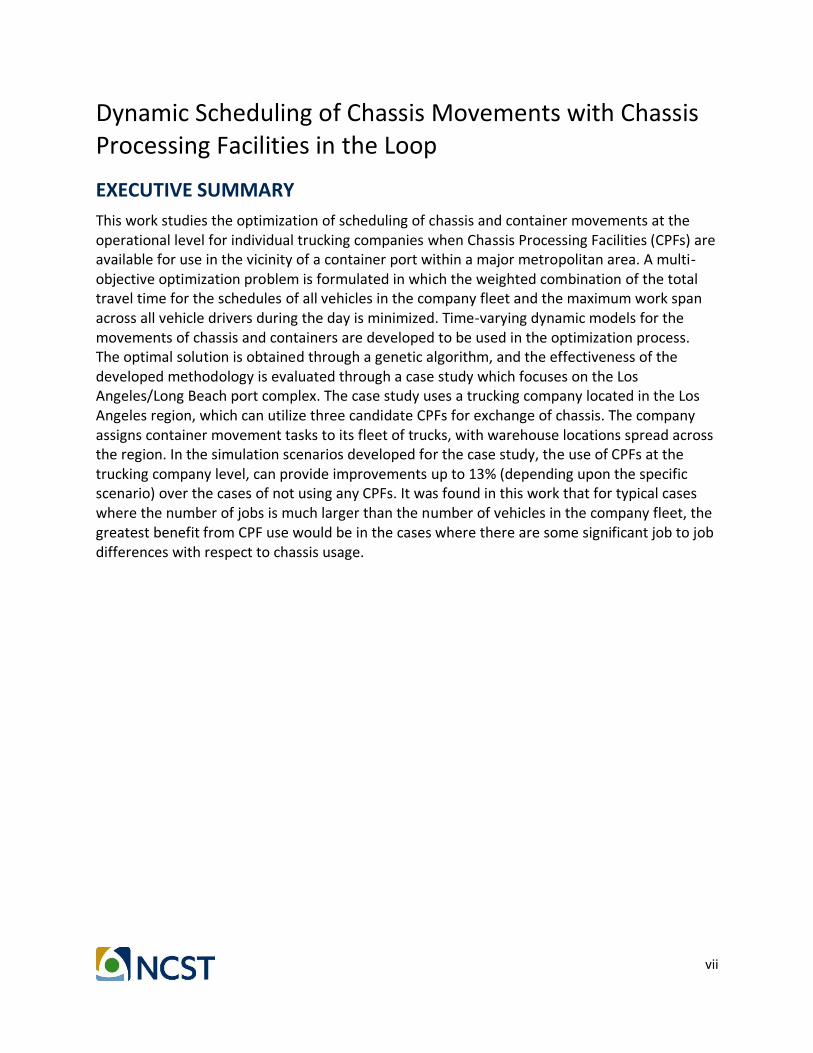
This work studies the optimization of scheduling of chassis and container movements at the operational level for individual trucking companies when Chassis Processing Facilities (CPFs) are available for use in the vicinity of a container port within a major metropolitan area. A multi-objective optimization problem is formulated in which the weighted combination of the total travel time for the schedules of all vehicles in the company fleet and the maximum work span across all vehicle drivers during the day is minimized. Time-varying dynamic models for the movements of chassis and containers are developed to be used in the optimization process. The optimal solution is obtained through a genetic algorithm, and the effectiveness of the developed methodology is evaluated through a case study which focuses on the Los Angeles/Long Beach port complex. The case study uses a trucking company located in the Los Angeles region, which can utilize three candidate CPFs for exchange of chassis. The company assigns container movement tasks to its fleet of trucks, with warehouse locations spread across the region. In the simulation scenarios developed for the case study, the use of CPFs at the trucking company level, can provide improvements up to 13% (depending upon the specific scenario) over the cases of not using any CPFs. It was found in this work that for typical cases where the number of jobs is much larger than the number of vehicles in the company fleet, the greatest benefit from CPF use would be in the cases where there are some significant job to job differences with respect to chassis usage.

1
1. Introduction
According to the World Bank, world ports handled more than 700 million 20-foot equivalent units (TEUs) of containers in 2016 (Figure 1 and Figure 2), [1]. Figure 1 shows that the global container traffic has increased over 200% from 2000 to 2016. Figure 2 shows that the United States (and China) have the highest levels of container traffic in the world.
Figure 1. World’s container port traffic in TEU (2000-2016)

2
Figure 2. Container port traffic in TEU by country (2016)
In fact, the busiest container port in the U.S. is the port complex of Los Angeles and Long Beach. In 2015 the combined ports handled 15.4 million TEUs [2], [3]. This number represents a 56% increase since 2000 and is expected to grow even higher in the future. Since most of the containers in use are 40-foot units (FEU), the figure of 15.4 million TEUs corresponds to approximately 8.3 million individual container units (the conversion factor most widely used in the industry is: One Individual Container = 1.85 TEU, [4]).
This large volume of container trips results in traffic congestion, noise pollution, and greenhouse gas emissions in the areas around and within the ports [5]. Traffic congestion, in turn, impacts the local economy by decreasing reliability of delivery time for the imported goods, which forces local businesses to use more operators, equipment, distribution centers and inventory in order to deliver their end-products on time. One metric that can be used to assess the overall effectiveness of a proposed solution is the total travel time for trucks transporting goods from/to the ports during a given time period. This metric is correlated strongly with all of the items outlined above. Therefore, any concept which could minimize this total travel time can be expected to have a positive effect on all of these areas, [6], [7]. One such concept which could have a positive impact on total travel time, is the concept of Centralized Processing of Chassis.
A previous METRANS project performed by the principal investigators [8]; [9] developed an analytical framework for modeling and optimization of the concept of Centralized Processing of

3
Chassis around marine container terminals, with application to the Los Angeles/Long Beach port area. This concept revolves around an off-dock terminal (or several off-dock terminals), referred to as Chassis Processing Facilities (CPFs). A CPF is located close to the port, where trucks will go to exchange chassis, thereby reducing traffic at the marine terminals, resulting in reduced travel times for trucks and the potential of reduced emissions.

4
2. Background and Literature Review
2.1. POLB and POLA Complex
The combined twin ports of the Port of Long Beach (POLB) and Port of Los Angeles (POLA) create the largest container port complex in the US. Figure 3 shows the annual TEU throughput at the ports of Long Beach and Los Angeles for the period 1997-2016 [2], [3]. Although the explosive growth of the first ten years exhibited a slowdown after the recession of 2008, it has achieved quite a healthy recovery in the last few years reaching or surpassing its pre-recession levels. The numbers in Figure 3 include both loaded and empty units, destined for import or export.
Figure 4 shows the change in total annual TEU throughput for the combined ports. The yearly change over the last six years is positive. The total container throughput (import and export) through the POLA and POLB is expected to grow in the future, correlated with population increase, domestic demand for inexpensive manufactured goods, as well as global demand for US agricultural products, and improving competitiveness of US industry. Handling a large number of the necessary container transactions requires intensive management of operations, changes in transportation policy and modernized equipment.
Figure 3. Annual TEU throughput at POLB & POLA (1997-2017)

5
Figure 4. Annual change in TEU throughput for the combined ports (2012-2017)
2.2. Typical Transaction Types for Container Transport
In order to complete the export/import operations for containers to/from marine terminals the transporting trucks will perform a series of steps including: dropping off export containers; dropping off empty chassis used for exports; picking up chassis for imports; picking up import containers; and traveling between any locations necessary to complete these tasks [10], [11]. The most common transaction types for trucking companies at marine terminals are listed below.
Type 1: Single transaction export
Type 2: Single transaction import of grounded container (i.e. container not loaded on a chassis)
Type3: Single transaction import of wheeled container (i.e. container already loaded on chassis)
Type 4: Dual transaction export / import of grounded import
Type 5: Dual transaction export / import of wheeled import
Figure 5 shows the flow of bobtails, chassis and containers for transaction types 1-5 described above. The flows presented in Figure 5 depict the operations taking place between the in-gate and out-gate of the marine terminal. The truck’s point of origin or its final destination, which could be for example a warehouse or a parking space at the trucking company, are not depicted in the figure. The following list provides a detailed explanation of the operations taking place for each type of the five transactions.
6
• Type 1: Single transaction export. The bobtail leaves the trucking company (or its point of origin) with a chassis on which an export container is loaded. It arrives at the in-gate; enters the terminal; drops off the export container and the chassis in the marine terminal; passes through the out-gate and arrives at its final destination as a bobtail.
• Type 2: Single transaction import of grounded container. The bobtail arrives at the in-gate; picks up a chassis at the marine terminal; picks up an import container; passes through the out-gate and arrives at its final destination as a bobtail with a chassis and a container.
• Type 3: Single transaction import of wheeled container. The bobtail arrives at the in-gate; picks up a chassis which has already been loaded with an import container; passes through the out-gate and arrives at its final destination as a bobtail with a chassis and a container.
• Type 4: Dual transaction export / import of grounded import. The bobtail arrives at the in- gate with a chassis on which an export container is loaded; enters the terminal; drops off the export container; loads an import container to the chassis; passes through the out-gate and arrives at its final destination as a bobtail with a chassis and a container.
• Type 5: Dual transaction export / import of wheeled import. The bobtail arrives at the in- gate with a chassis on which an export container is loaded; enters the terminal; drops off the export container; drops off the chassis; picks up a chassis which has already been loaded with an import container; passes through the out-gate and arrives at its final destination as a bobtail with a chassis and a container.

7
Figure 5. Description of container transaction types at marine terminals

8
2.3. Problems Present at the POLB and POLA
Two of the key hurdles to overcome in managing POLB and POLA container imports and exports include chassis shortages and heavy traffic surrounding the port.
2.4. Shortage of Chassis
In the POLB and POLA, there are approximately 100,000 chassis available for leasing and transporting containers to and from warehouses, stores, factories, rail yards and container terminals [12]. Among these 100,000 chassis available to the trucking companies there are chassis supplied by various third party chassis leasing companies. However, terminals within the ports do not always have chassis available from each company. At times chassis required by the trucks are either not available anywhere in the terminal or are dislocated and need to be repositioned.
Prior to 2014 chassis companies did not work together or have a neutral chassis pool, and shortages and dislocations of chassis occurred frequently. Trucks would often be required to travel between terminals and perform additional trips to pick up or drop-off chassis at specific locations in addition to picking up and dropping off the containers for export and import. This was a lengthy and cumbersome process and generated additional queues at each terminal [13].
The shortage of chassis can significantly lengthen truck turn times, causing additional cost for trucking companies and increasing emissions at the port. Lack of chassis could also cause containers to be kept at the carrier ship for a prolonged time, resulting in the accumulation of storage fees. In addition, when containers are not discharged in a timely manner, the shippers face a congested space in their area of operation. This can, in turn, force shippers to rent additional storage area, leading to more expensive carrying cost and delayed delivery time [13]. According to POLA/POLB terminal operators and PierPass officials (2014) one of the core reasons for port congestion is lack of chassis [10].
2.5. Traffic Congestion
Traffic congestion around the port is also contributing to the slowdown of port operations. At the POLB and POLA trucks are coming from many locations to drop-off or pick up containers and chassis, where the freeways that truck drivers must use to access the port are also used heavily by commuters traveling through the densely populated area surrounding Los Angeles. [14]. The most heavily used freeway to get to and from the POLB and POLA is California Interstate 710 (I-710). I-710 has, for the most part, four lanes, heavily packed with trucks and commuter vehicles during rush hours, causing major congestion problems in the vicinity of the ports.
As the American economy expands, there is more demand for commercial operations, increased freight, and increased numbers of foreign commercial partners. This gives rise to recurring congestion at freight bottlenecks, creating a conflict between freight and passenger service. Moreover, as demands for trading partners increase, more freight ships will be docked

9
at the ports. Handling more transactions also means that the ports will have to increase their processing capacity. This increase will undoubtedly cause the entrance to the port and the areas within the port itself to be heavily congested as well [14].
Congestion in and outside of the port is detrimental to the economy in Southern California as well as that of the US as a whole. When there is additional congestion, port operators take much longer to unload cargo ships. Supply chains carrying goods through the POLB and POLA can then become slowed to the point where some retailers find it necessary to redirect their goods. The goods are then redirected by sea or air to other ports on the East Coast where they can be further distributed, resulting in reduced income for the surrounding area as well as additional costs for the retailers [15] [16].
2.6. Chassis Leasing and the Gray Chassis Pool
In late 2014, three chassis leasing companies including Direct Chassis Link, Inc. (DCLI), Trans-Pacific (TRAPAC) Intermodal and Flexi-Van, along with a container terminal operator SSA Marine, (formerly Stevedoring Services in America), decided to develop a solution to the chassis shortage problem. The four companies own about 95% of the total 100,000 chassis in use in the POLA/POLB area. Figure 6 shows the chassis ownership distribution among the four companies, as of 2014. The proposed solution to the chassis shortage problem came in the form of a chassis management model known as “Gray Chassis Pool” or “Pools of Pools (POP)” [10] [12].
Figure 6. Chassis ownership in the POLB/POLA area
The POP is a neutral, interoperable chassis pool that was launched in February 2015, from DCLI, TRAC Intermodal and Flexi-Van, in cooperation with the POLA, POLB and SSA Marine. Their

10
chassis are pooled together to provide a more efficient way of obtaining chassis for trucking companies, which are able to use the chassis from any of the chassis companies interchangeably. Thus, a trucker can pick any chassis from the POP and drop it off at any designed POP storage area without having to worry about returning chassis to the same exact location. Since truckers have access to any chassis, it allows for a smoother operation at the port and fewer inefficiencies in chassis-related operations. However, the pools still remain commercially independent and are in competition with one another. A third party service provider manages the billing and other proprietary information among these pools [17].
Nonetheless, even with the improved flexibility, interoperability and efficiency which the POP has introduced, the port still suffers some repositioning issues and the heavy traffic congestion problems remain.
2.7. Centralized Processing of Chassis
The concept of Centralized Processing of Chassis was introduced as one method for improving travel times associated with container retrieval. This concept was introduced in Europe as the Chassis Exchange Terminal (CET) [18]. In the CET concept, the centralized processing of chassis was defined as an off- dock terminal (or a number of off-dock terminals) located close to the port, where trucks would go to retrieve imports or drop-off exports instead of unloading and loading containers at the marine terminal.
The first step in the operation with the CET involved a container being loaded onto a chassis at the marine terminal. The second step included the chassis transport to the CET during off-peak hours, for example at night time. The last step in the operation was when a truck carrying a chassis with a container drives into the CET. At this point, the truck would exchange the chassis it brought into the CET with another chassis and container, which has already been transported to the CET during the second step. The exchange operation involves unhooking a chassis and hooking up another one at the CET. This is much simpler, more efficient, and a lot faster operation than the operation of unloading and loading containers and performing chassis exchanges at a regular marine terminal.

11
3. Problem Description
3.1. Problem
In the previous METRANS project performed by the principal investigators [8], the concept of CPFs and the possibility of using it to improve travel time for trucks was studied.
The previous study established and quantified the benefits to the overall traffic network that can be achieved through the use of CPFs. A methodology for determining the optimal locations and number of CPFs was developed and tested on a case study focusing specifically on the ports of Los Angeles and Long Beach. In that project it was shown that a reduction of up to 20% in total travel time can be achieved when using the CPFs, as compared to using only the marine terminals. The results for the particular case study also showed that using up to three of the potential CPFs provides significant improvements to total travel time, but using more than three CPFs has insignificant additional benefits.
While the benefits at the system/strategic level were established in the previous project, the question of how best to take advantage of the CPF facilities at the operational level has remained open. With further refinement to develop an approach to proactively (and dynamically) schedule drayage operations from a trucking company’s point of view, cost as well as traffic congestion, noise and emissions can be further reduced.
3.2. Objectives
As mentioned above, the focus of the present study is to investigate the effectiveness of the CPF concept at the operational level. The main objective herein is to develop an analytical framework for dynamic modeling of chassis movements and to investigate optimization techniques for scheduling the tasks and minimizing the total travel time of the drivers from a particular trucking company’s point of view, when several CPFs are available for use. The methodologies to be developed will contribute greatly to improving trucking companies’ daily operations, and as a result will improve traffic conditions in the areas surrounding the ports.
The plan is to investigate both the temporal and spatial components of the CPF concept. That is, in addition to the optimal location of CPFs, the scheduling of individual trucks and the time when a CPF will be visited for exchanging of chassis will be considered. These two factors are simultaneously incorporated into the models to optimally determine the schedule for each truck.
At the initial phase, the methodology developed by the Principal Investigators (PI)s in their previous work [8] will be used to determine the number and optimal locations of CPFs.
At the next phase, the set of all tasks that must be completed by a particular trucking company within a day will be formalized and incorporated into the optimization problem formulation.

12
In order to complete the export/import operations for containers to/from marine terminals the transporting trucks will perform a series of steps [10], [11], including:
• dropping off export containers
• dropping off empty chassis used for exports
• picking up chassis for imports; picking up import containers
• traveling between any locations necessary to complete these tasks
Note that depending upon the destination container configurations and sequence of tasks this would allow for any of the five most common transaction types in marine terminals presented in Section 2.2.
3.3. Formal definition of a job
Given a particular trucking company (TC), we assume that the set of all daily tasks that need to be completed are known, and each of these tasks consists of moving one container between one of the customer warehouses (WH)s and marine terminals (MT)s, or vice-versa, with or without the use of CPFs. In the sequel the definition of a job will be formalized. A job, which is a task, consists of a container movement with the following attributes:
i. Origin. The origin of a job will be one of the WHs if it transports an export container, or one of the MTs if it is an import container.
ii. Destination. Similar to the origin, the destination of a job will be one of the MTs if it is an export container or one of the WHs if it is an import activity.
iii. Origin Container Configuration. This refers to the state of the container at the origin (Grounded or Wheeled). It is noted that for our purposes only two states for this attribute are considered.
iv. Destination Container Configuration. This refers to the state of the container at the destination (Grounded or Wheeled).
v. Earliest Allowable Completion Time for the job.
vi. Latest Allowable Completion Time for the job.
The general concept of a series of jobs, i.e. vehicle routing from an individual trucking company’s point of view including the possible use of CPFs, is illustrated in Figure 7 and Table 1. A particular trucking company labeled as TC in Figure 7, needs to complete three jobs using the M trucks (or vehicles) available, which are denoted as 𝑉1, … 𝑉𝑀. It is assumed that the M vehicles available to the TC will be servicing a variety of customer locations and marine terminals. The L marine terminal locations are given as 𝑀𝑇1, … 𝑀𝑇𝐿 and the J customer locations which the trucking company is servicing are generically labeled as warehouses 𝑊𝐻1, …𝑊𝐻𝐽.

13
The set of jobs assigned to 𝑉𝑚 is shown in Table 1, with the resultant path illustrated in Figure 7. In this example, three jobs are to be completed (Job1 is an export; Jobs 2 and 3 are imports).
• Job 1 consists of picking up a wheeled export container from warehouse 𝑊𝐻1 and transporting it to marine terminal 𝑀𝑇𝑙 , where it will be left in a grounded configuration.
• Job 2 is to pick up a grounded import container from marine terminal 𝑀𝑇𝐿 and transport it to warehouse 𝑊𝐻𝐽 , where it will be left in a wheeled configuration.
• Job 3 is to pick up a grounded import container from marine terminal 𝑀𝑇1 and transport it to warehouse 𝑊𝐻𝐽 , where it will be left in a wheeled configuration. However, the
transport truck does not have a chassis, since it left it with the container at warehouse 𝑊𝐻𝐽 during completion of Job 2, hence Job 3 will require a visit to the kth CPF, 𝐶𝑃𝐹𝑘, to
pick up an available chassis, as outlined in Figure 7.
Figure 7. Example schematic of vehicle routing problem with CPFs

14
Table 1. Schedule example for vehicle 𝑽𝑽𝑽𝑽
Attribute Job 1 Job 2 Job 3 (i) Origin 𝑊𝐻1 𝑀𝑇𝐿 𝑀𝑇1 (ii) Destination 𝑀𝑇𝑙 𝑊𝐻J 𝑊𝐻j (iii) Origin Container
Configuration Wheeled Grounded Grounded
(iv) Destination Container Configuration Grounded Wheeled Wheeled
(v) Earliest Allowable Completion Time for job
8:00 AM 8:00 AM 8:00 AM
(vi) Latest Allowable Completion Time for job
5:00 PM 5:00 PM 5:00 PM
The general process flow for any vehicle schedule for a given sequence of jobs is shown in Figure 8. For each job there are three basic components: job preparation, job pick-up, and job drop-off.
• Job preparation involves assessing whether the vehicle is ready for the current job and, if necessary, picking up a chassis if one is needed for a grounded transaction or dropping off a chassis if the transaction is with a wheeled container.
• Job pick up involves retrieving a wheeled or grounded container from either a WH for an export or a MT for an import.
• Job drop off involves dropping off a wheeled or grounded container from either a MT for an export or a WH for an import.
Job assignment to each of the vehicles and optimization thereof is covered in more detail in the following sections.

15
Figure 8. General process flow for vehicle schedule
16
4. Analytical Models and Optimization
In this section, a general analytical framework for the scheduling of jobs for a trucking company is developed, assuming that CPFs are available to be used. The optimal vehicle scheduling will be identified within this particular framework.
Due to recent changes in chassis leasing policies, such as the introduction of the grey chassis pool in the ports of Long Beach and Los Angeles, for the purpose of this analysis it is assumed that chassis of similar types are interchangeable, and transactions do not need to take into account chassis ownership.
Given:
• the location of the trucking company 𝑇𝐶, which must complete the particular tasks
• the locations of the marine terminals, 𝑀𝑇𝑙 , 𝑙 = 1, … , 𝐿
• the locations of the customers, or “warehouses” 𝑊𝐻𝑗 , 𝑗 = 1, … , 𝐽
• the locations of potential sites for chassis processing facilities 𝐶𝑃𝐹𝑘, 𝑘 = 1, … , 𝐾,
• a set of import and export jobs that need to be completed between 𝑊𝐻𝑗, 𝑗 = 1, … , 𝐽,
and 𝑀𝑇𝑙, 𝑙 = 1, … , 𝐿 , where each job is determined by its own particular attributes as defined previously in Section 3.3
• a set of vehicles (trucks) to carry out the jobs
• the maximum allowable work span for any given vehicle
The objective herein is to minimize the weighted combination of:
• the total travel time for all vehicles
• the work span needed to finish all jobs
As defined above, the problem is a multi-objective optimization problem. The purpose of minimizing both total travel time and work span is to provide a more realistic model for the trucking company’s priorities, where the goal is to minimize (a) the direct hourly costs for completion of jobs, represented by the total travel time for all vehicles, while (b) spreading the jobs as evenly as possible among the vehicle drivers, represented by the work span to finish all jobs. The equal spreading of jobs between drivers is necessary since typically a given staff of drivers is available already to the trucking company to perform the jobs for the day. Therefore, unequally assigned work would result in staff who, depending upon the pay structure, are either being underutilized (and overpaid) or paid for minimal hours of work so that the trucking company is not providing a reliable income to their workers and may not be able to maintain trained and available staff.
17
4.1. Problem Formulation
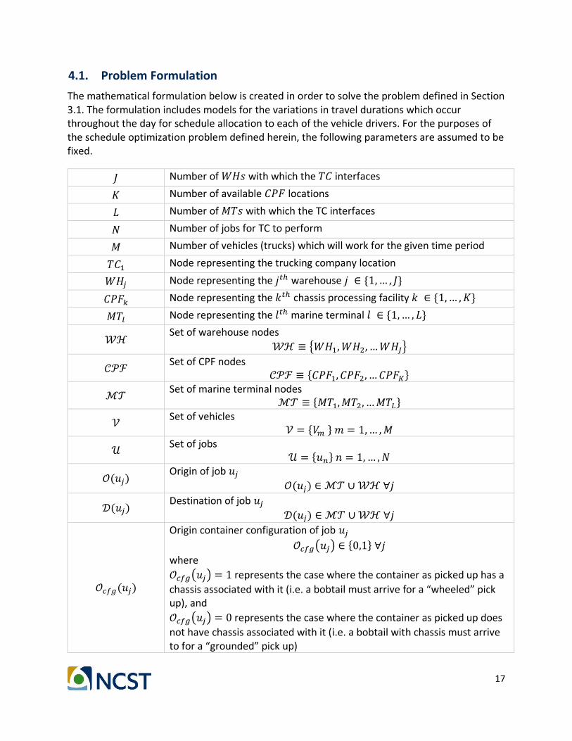
The mathematical formulation below is created in order to solve the problem defined in Section 3.1. The formulation includes models for the variations in travel durations which occur throughout the day for schedule allocation to each of the vehicle drivers. For the purposes of the schedule optimization problem defined herein, the following parameters are assumed to be fixed.
𝐽 Number of 𝑊𝐻𝑠 with which the 𝑇𝐶 interfaces
𝐾 Number of available 𝐶𝑃𝐹 locations
𝐿 Number of 𝑀𝑇𝑠 with which the TC interfaces
𝑁 Number of jobs for TC to perform
𝑀 Number of vehicles (trucks) which will work for the given time period
𝑇𝐶1 Node representing the trucking company location
𝑊𝐻𝑗 Node representing the 𝑗𝑡ℎ warehouse 𝑗 ∈ {1,… , 𝐽}
𝐶𝑃𝐹𝑘 Node representing the 𝑘𝑡ℎ chassis processing facility 𝑘 ∈ {1,… , 𝐾}
𝑀𝑇𝑙 Node representing the 𝑙𝑡ℎ marine terminal 𝑙 ∈ {1,… , 𝐿}
𝒲ℋ Set of warehouse nodes
𝒲ℋ ≡ {𝑊𝐻1,𝑊𝐻2, …𝑊𝐻𝐽}
𝒞𝒫ℱ Set of CPF nodes
𝒞𝒫ℱ ≡ {𝐶𝑃𝐹1, 𝐶𝑃𝐹2, … 𝐶𝑃𝐹𝐾}
ℳ𝒯 Set of marine terminal nodes
ℳ𝒯 ≡ {𝑀𝑇1,𝑀𝑇2, …𝑀𝑇𝐿}
𝒱 Set of vehicles
𝒱 = {𝑉𝑚 } 𝑚 = 1,… ,𝑀
𝒰 Set of jobs
𝒰 = {𝑢𝑛} 𝑛 = 1,… , 𝑁
𝒪(𝑢𝑗) Origin of job 𝑢𝑗
𝒪(𝑢𝑗) ∈ ℳ𝒯 ∪ 𝒲ℋ ∀𝑗
𝒟(𝑢𝑗) Destination of job 𝑢𝑗
𝒟(𝑢𝑗) ∈ ℳ𝒯 ∪ 𝒲ℋ ∀𝑗
𝒪𝑐𝑓𝑔(𝑢𝑗)
Origin container configuration of job 𝑢𝑗
𝒪𝑐𝑓𝑔(𝑢𝑗) ∈ {0,1} ∀𝑗
where
𝒪𝑐𝑓𝑔(𝑢𝑗) = 1 represents the case where the container as picked up has a
chassis associated with it (i.e. a bobtail must arrive for a “wheeled” pick up), and
𝒪𝑐𝑓𝑔(𝑢𝑗) = 0 represents the case where the container as picked up does
not have chassis associated with it (i.e. a bobtail with chassis must arrive to for a “grounded” pick up)
18
𝒟𝑐𝑓𝑔(𝑢𝑗)
Destination container configuration of job 𝑢𝑗
𝒟𝑐𝑓𝑔(𝑢𝑗) ∈ {0,1} ∀𝑗
where
𝒟𝑐𝑓𝑔(𝑢𝑗) = 1 represents the case where the container as dropped off has
a chassis associated with it (i.e. the bobtail will deliver both chassis and container to complete a “wheeled” drop-off), and
𝒟𝑐𝑓𝑔(𝑢𝑗) = 0 represents the case where the container as dropped off
does not have chassis associated with it (i.e. the bobtail will deliver only the container and leave with the chassis to complete a “grounded” drop-off)
𝑠𝑚,𝑖 The ith job in vehicle 𝑉𝑚’s schedule:
𝑠𝑚,𝑖 ∈ 𝒰 ∀ 𝑚, 𝑖 ∈ ℕ∗
𝑠𝑚 The schedule of vehicle 𝑉𝑚, sm ≡ {𝑠𝑚,1 …𝑠𝑚,𝑘}
𝑡𝑡𝑜𝑡(sm,i) The completion time for job sm,i
𝒯𝑚𝑎𝑥(𝑢𝑗) Latest allowable completion time for job uj
𝒯𝑚𝑖𝑛(𝑢𝑗) Earliest allowable completion time for job uj
𝑇𝑊𝑆𝑚𝑎𝑥 Maximum allowed work span
𝑡𝑛𝑜𝑑𝑒(𝑥𝑖, xj, 𝑡𝑘) The time to get from node 𝑥𝑖 to node 𝑥𝑗 at time 𝑡𝑘
𝑃(𝑥) Processing time for chassis retrieval / drop-off at node 𝑥,
𝑥 ∈ ℳ𝒯 ∪ 𝒲ℋ
𝑇𝑤ℎ Time to pick up or drop-off wheeled container
𝑇𝑔𝑛𝑑 Time to pick up or drop-off grounded container
𝑡0 Initial time for vehicle departure
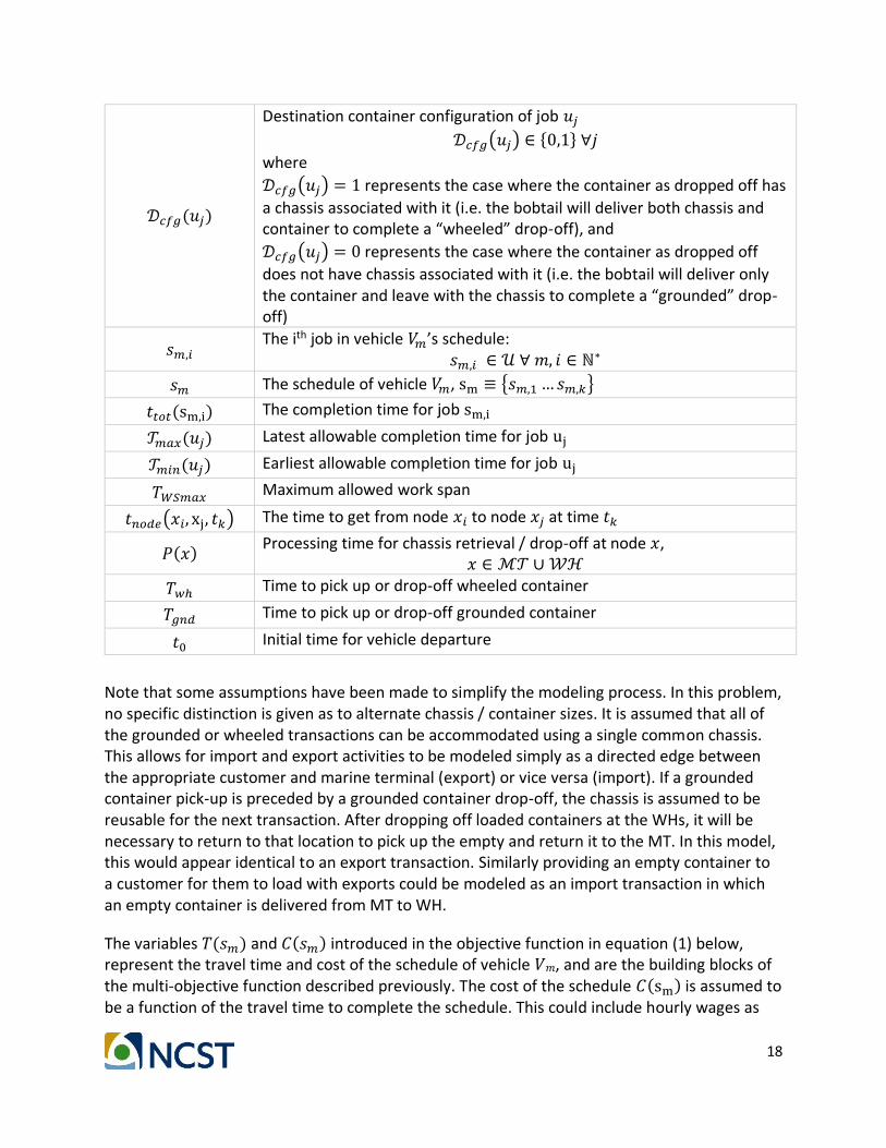
Note that some assumptions have been made to simplify the modeling process. In this problem, no specific distinction is given as to alternate chassis / container sizes. It is assumed that all of the grounded or wheeled transactions can be accommodated using a single common chassis. This allows for import and export activities to be modeled simply as a directed edge between the appropriate customer and marine terminal (export) or vice versa (import). If a grounded container pick-up is preceded by a grounded container drop-off, the chassis is assumed to be reusable for the next transaction. After dropping off loaded containers at the WHs, it will be necessary to return to that location to pick up the empty and return it to the MT. In this model, this would appear identical to an export transaction. Similarly providing an empty container to a customer for them to load with exports could be modeled as an import transaction in which an empty container is delivered from MT to WH.
The variables 𝑇(𝑠𝑚) and 𝐶(𝑠𝑚) introduced in the objective function in equation (1) below, represent the travel time and cost of the schedule of vehicle 𝑉𝑚, and are the building blocks of the multi-objective function described previously. The cost of the schedule 𝐶(sm) is assumed to be a function of the travel time to complete the schedule. This could include hourly wages as

19
well as other costs to the trucking company associated with supporting a given vehicle schedule.
The objective function is given by:
min ∑ 𝐶(𝑠𝑚)
𝑀
𝑚=1
+ 𝜇 max𝑚=1,…,𝑀
𝑇(𝑠𝑚) (1)
s.t. 𝒯𝑚𝑖𝑛(sm,i) ≤ 𝑡𝑡𝑜𝑡(sm,i) ≤ 𝒯𝑚𝑎𝑥(sm,i) 𝑚 = 1, … ,𝑀
𝑖 = 1,… , |𝑠𝑚| (2)
|sm| ≥ 1 𝑚 = 1, … ,𝑀 (3)
𝑠𝑖⋂𝑠𝑗 = ∅ ∀ 𝑖 ≠ 𝑗 (4)
⋃ 𝑠𝑚
𝑀
𝑚=1
= 𝒰 𝑚 = 1, … ,𝑀 (5)
For a given job, the total completion time is given by
𝑡𝑡𝑜𝑡(sm,i) = max (𝑡∗ + 𝑡𝑛𝑜𝑑𝑒(𝒪(𝑠𝑚,𝑖),𝒟(𝑠𝑚,𝑖), 𝑡∗)
+ (𝒟𝑐𝑓𝑔(𝑠𝑚,𝑖) = 1 → 𝑇𝑤ℎ)⋀(𝒟𝑐𝑓𝑔(𝑠𝑚,𝑖) = 0
→ 𝑇𝑔𝑛𝑑), 𝒯𝑚𝑖𝑛(sm,i))
𝑚 = 1, … ,𝑀 𝑖 = 2,… , |𝑠𝑚|
where
𝑡∗ = 𝑡𝑡𝑜𝑡(𝑠𝑚,𝑖−1) + 𝑡𝑗𝑜𝑏 (𝑠𝑚,𝑖−1, 𝑠𝑚,𝑖 , 𝑡𝑡𝑜𝑡(𝑠𝑚,𝑖−1))
+ (𝒪𝑐𝑓𝑔(𝑠𝑚,𝑖) = 1 → 𝑇𝑤ℎ)⋀(𝒪𝑐𝑓𝑔(𝑠𝑚,𝑖) = 0 → 𝑇𝑔𝑛𝑑)
(6)
𝑡𝑡𝑜𝑡(sm,1) = max (𝑡† + 𝑡𝑛𝑜𝑑𝑒(𝒪(𝑠𝑚,1),𝒟(𝑠𝑚,1), 𝑡†)
+ (𝒟𝑐𝑓𝑔(𝑠𝑚,1) = 1 → 𝑇𝑤ℎ)⋀(𝒟𝑐𝑓𝑔(𝑠𝑚,1) = 0
→ 𝑇𝑔𝑛𝑑), 𝒯𝑚𝑖𝑛(𝑠𝑚,1))
𝑚 = 1,… ,𝑀 where
𝑡† = 𝑡0 + 𝑡𝑗𝑜𝑏(𝑇𝐶𝑗𝑜𝑏, 𝑠𝑚,𝑖 , 𝑡0)
+ (𝒪𝑐𝑓𝑔(𝑠𝑚,1) = 1 → 𝑇𝑤ℎ)⋀(𝒪𝑐𝑓𝑔(𝑠𝑚,1) = 0 → 𝑇𝑔𝑛𝑑)
(7)

20
where TCjob is a “dummy” job defined such that
𝒪(TCjob) = 𝑇𝐶1
𝒟(TCjob) = 𝑇𝐶1
𝒪cfg(TCjob) = 1
𝒟cfg(TCjob) = 1
𝒯𝑚𝑖𝑛(TCjob) = −∞
𝒯𝑚𝑎𝑥(TCjob) = ∞
(8)
and
𝑡𝑗𝑜𝑏(𝑢𝑖 , 𝑢𝑗 , 𝑡𝑘) is the time to get from job 𝑢𝑖 to job 𝑢𝑗 at time 𝑡𝑘 which is
given by
𝑡𝑗𝑜𝑏(𝑢𝑖 , 𝑢𝑗 , 𝑡𝑘) =
((𝒟cfg(ui) = 𝒪cfg(uj)) → 𝑡𝑛𝑜𝑑𝑒(𝒟(ui),𝒪(uj), 𝑡𝑘))⋀ ((𝒟cfg(ui) ≠ 𝒪cfg(uj))
→ 𝑡‡ + 𝑡𝑛𝑜𝑑𝑒(𝑥𝑜𝑝𝑡(𝒟(ui),𝒪(uj), 𝑡𝑘),𝒪(uj), 𝑡𝑘 + 𝑡‡))
where 𝑥𝑜𝑝𝑡(𝑥𝑖 , 𝑥𝑗 , 𝑡𝑘) is the optimum chassis processing location which
results in minimal travel / chassis processing time when traveling between nodes 𝑥𝑖 and 𝑥𝑗 at time 𝑡𝑘 and
𝑡‡ = 𝑡𝑛𝑜𝑑𝑒(𝒟(ui), 𝑥𝑜𝑝𝑡(𝒟(ui),𝒪(uj), 𝑡𝑘), 𝑡𝑘) + 𝑃 (𝑥𝑜𝑝𝑡(𝒟(ui), 𝒪(uj), 𝑡𝑘))
(9)
Using the recursive formula above, the travel time to complete vehicle 𝑣𝑚 ’s schedule 𝑇(sm) is then given by:
𝑇(sm) = 𝑡𝑡𝑜𝑡(sm,|sm|) + 𝑡𝑗𝑜𝑏 (sm,|sm|, 𝑇𝐶𝑗𝑜𝑏 , 𝑡𝑡𝑜𝑡(sm,|sm|)) − 𝑡0
𝑚 = 1, … ,𝑀 (10)
The cost of the schedule 𝐶(sm) is then assumed to be a function of the travel time to complete the schedule as noted below. This function could include the hourly wage of the driver for standard hourly pay, nonlinear elements to address overtime pay, as well as other costs to the trucking company associated with supporting a given vehicle schedule such as average costs due to vehicle maintenance.
𝐶(sm) = 𝑓(𝑇(sm)) 𝑚 = 1,… ,𝑀 (11)
21
4.2. Optimization Methodology
In this project, an optimization methodology is developed to find the optimal solution to the scheduling problem, as described above. As with most scheduling problems, the problem defined above is NP hard. In addition, as compared to most typical scheduling problems, there are a few factors which add further complexity to the current problem, including:
• The current problem is a multi-objective optimization problem. One objective is to minimize the total cost; the other objective is to minimize the maximum work span of vehicles.
• When the job schedule is such that it includes moving a chassis to/from CPFs, the choice of CPF is flexible, increasing the size of the potential solution space.
• There is a time window associated with each job.
In order to perform the optimization for this problem, metaheuristic methods are leveraged which can provide effective and efficient solutions. These problem-independent techniques include approaches which operate on a single solution such as simulated annealing or tabu searches, as well as approaches which operate on a set of solutions such as genetic algorithms or particle swarm optimization. Various metaheuristics were assessed to identify a suitable approach to solve the problem, which have in turn been adjusted according to the problem at hand to fine-tune its intrinsic parameters. After careful consideration and evaluation, the genetic algorithm approach was chosen as the metaheuristic to be used.
4.3. Genetic Algorithm Overview
With the genetic algorithm, our goal is to minimize the weighted combination of the total travel time for all vehicles and the work span needed to finish all jobs by allocating a fixed set of jobs between WHs and MTs to a given fleet of vehicles. The optimal configuration is described by the job allocation. The problem is such that an ordered set of jobs allocated to each of the vehicles defines any given solution.
This ordered set serves as the chromosome in the genetic algorithm. Each of the individual job entries in this set which describe which vehicle is responsible for the job and when it occurs in that vehicle’s schedule then serves as a gene. An example of a set of genes and single chromosome is shown in Figure 9 below.

22
Figure 9. Example of chromosomes and genes used in the genetic algorithm
Given these chromosomes, the process by which the genetic algorithm is implemented to optimize the objective function is shown in Figure 10. The example in Figure 10 is based on scheduling ten vehicles to complete sixty jobs during a given day. Some of the final settings used in the algorithm including population, crossover percentage, elite count, and termination criteria are indicated in the figure. The basic steps include:
• initialization (where the initial population is generated)
• selection (in which the fitness of the population is evaluated), and in our case an objective function which calculates reliability
• the generation of children based upon the selection criteria
• the implementation of crossover and mutation algorithms.
The entire process is then repeated until the termination criteria have been reached.

23
Figure 10. Genetic algorithm overview
4.4. Initial Population
Each of the chromosomes in the initial population for the genetic algorithm was generated using one of four separate algorithms, including two nearest neighbor algorithms and two random permutation algorithms. Note that all four algorithms were built to force the permutations of the jobs spread across the vehicle schedules within a given chromosome to be such that the constraints of equations (3), (4), and (5) would all be met.
4.4.1. Nearest Neighbor Algorithm 1
The first of the chromosomes in the initial population was generated using a nearest neighbor algorithm which equally distributed jobs between all vehicles. This algorithm sequenced through each of the vehicle schedules assigning jobs in the sequence 𝑠1,1, 𝑠2,1, … 𝑠𝑀,1, 𝑠1,2, 𝑠2,2, … 𝑠𝑀,2 … until all jobs were assigned, where in each case 𝑠𝑚,𝑖 𝑖 was
selected such that 𝑡𝑗𝑜𝑏(𝑠𝑚,𝑖−1, 𝑠𝑚,𝑖 , 𝑡𝑡𝑜𝑡(sm,i−1)) was minimized, and where 𝑠𝑚,0 ≡ 𝑇𝐶𝑗𝑜𝑏 and
𝑡𝑡𝑜𝑡(𝑇𝐶𝑗𝑜𝑏) = 𝑡0. An example result for this algorithm is shown in Figure 11.

24
Figure 11. Nearest Neighbor Algorithm 1 Example Output
Row 𝒔𝒎 represents the schedule of vehicle 𝑽𝒎 for the day. Square 𝒖𝒏 represents the 𝒏𝒕𝒉 job that the trucking company has to complete, from a total of 𝑵 jobs for the day. Job 𝒖𝒏 contains all the attributes of a
job as defined previously. The 𝒊𝒕𝒉 column represents the 𝒊𝒕𝒉 task in sequence that a vehicle has to perform. The “nearest neighbor algorithm 1” assigns the jobs uniformly to all available vehicles.
4.4.2. Nearest Neighbor Algorithm 2
The second of the chromosomes in the initial population was generated using a nearest neighbor algorithm which assigned one job to each of the vehicles and then assigned all remaining jobs to a single vehicle. This algorithm sequenced through each of the vehicle schedules assigning jobs in the sequence 𝑠1,1, 𝑠2,1, … 𝑠𝑀,1, 𝑠1,2, 𝑠1,3, 𝑠1,4 … 𝑠1,𝑁−𝑀+1 until all jobs were assigned, such that in each case 𝑠𝑚,𝑖 was once again selected such that
𝑡𝑗𝑜𝑏 (𝑠𝑚,𝑖−1, 𝑠𝑚,𝑖 , 𝑡𝑡𝑜𝑡(sm,i−1)) was minimized. An example result for this algorithm is shown in
Error! Reference source not found..

25
Figure 12. Nearest Neighbor Algorithm 2 Example Output Row 𝒔𝟏 represents the schedule of vehicle 𝑽𝟏 for the day. Rows 𝒔𝟐 − 𝒔𝟏𝟎 represent the schedules of vehicles {𝑽𝟐, 𝑽𝟑,⋯𝑽𝟏𝟎 }. The “nearest neighbor algorithm 2” assigns only one job to each of the vehicles {𝑽𝟐, 𝑽𝟑,⋯𝑽𝟏𝟎 }, and the remaining 51 jobs to vehicle 𝑽𝟏. Note that for reasons of simplicity and clarity, only a few of the 51 jobs for 𝒔𝟏 are shown in the figure.
4.4.3. Random Permutation Algorithm 1
The remaining chromosomes in the initial population were generated using two different algorithms which provide random permutations of the job sequence, with each algorithm generating ~50% of the resultant population. In the first random permutation algorithm, jobs were distributed equally across all of the available vehicles. An example result for this algorithm is shown in Figure 13.

26
Figure 13. Random Permutation Algorithm 1 Example Output
Row 𝒔𝒎 represents the schedule of vehicle 𝑽𝒎 for the day. Square 𝒖𝒏 represents the 𝒏𝒕𝒉 job that the trucking company has to complete, from a total of 𝑵 jobs for the day. Job 𝒖𝒏 contains all the attributes of a job as defined previously. The 𝒊𝒕𝒉 column represents the 𝒊𝒕𝒉 task in sequence that a vehicle has to perform. The “random permutation algorithm 1” assigns the jobs uniformly to all available vehicles.
Note that in the example above 𝑁/𝑀 is an integer, which allows equal spreading of jobs between all vehicles. However, the algorithm was written so that if this were not the case the first 𝑁 𝑚𝑜𝑑𝑢𝑙𝑜 𝑀 vehicles would be allocated ⌈𝑁/𝑀⌉ jobs, while the final 𝑀 − (𝑁 𝑚𝑜𝑑𝑢𝑙𝑜 𝑀) vehicles would be allocated ⌊𝑁/𝑀⌋. For example, if 𝑁 = 62 and 𝑀 = 10, the first 62 𝑚𝑜𝑑𝑢𝑙𝑜 10 = 2 vehicles are allocated ⌈62/10⌉ = 7 jobs, while the final 8 vehicles are allocated ⌊62/10⌋ = 6 jobs.
4.4.4. Random Permutation Algorithm 2
The other random permutation algorithm first randomly assigned a single job to each of the M vehicles, in order to force meeting the constraint of equation (3), and then randomly distributed the remaining jobs between all vehicles without any attempt to force an equal distribution. An example result for this algorithm is shown in Figure 14.

27
Figure 14. Random Permutation Algorithm 2 Example Output
Row 𝒔𝒎 represents the schedule of vehicle 𝑽𝒎 for the day. Square 𝒖𝒏 represents the 𝒏𝒕𝒉 job that the trucking company has to complete, from a total of 𝑵 jobs for the day. Job 𝒖𝒏 contains all the attributes of a
job as defined previously. The 𝒊𝒕𝒉 column represents the 𝒊𝒕𝒉 task in sequence that a vehicle has to perform. The “random permutation algorithm 2” first assigns one job to each of the vehicles {𝑽𝟏, 𝑽𝟐, ⋯𝑽𝟏𝟎, }, and then it assigns the remaining jobs randomly to each vehicle.
4.5. Fitness Function
In order to compare the quality of different chromosomes within the population, our fitness function for every chromosome represents the weighted sum of the total travel time for all vehicles and the work span needed to finish all jobs, which is calculated according to the algorithm described in Section Error! Reference source not found.. In addition, when calculating the fitness, constraint checks according to the optimization algorithm were performed to evaluate each chromosome’s validity. In the case that a chromosome is passed to the fitness function which fails any of the validity checks, the fitness value is not calculated and the chromosome’s fitness value is set to infinity.
4.6. Crossover Function
The crossover function should be chosen so that when low cost topologies are combined, they tend to produce low cost descendants. The crossover function implemented alternates between the two parents’ job sequences at the individual vehicle level to build a solution such
28
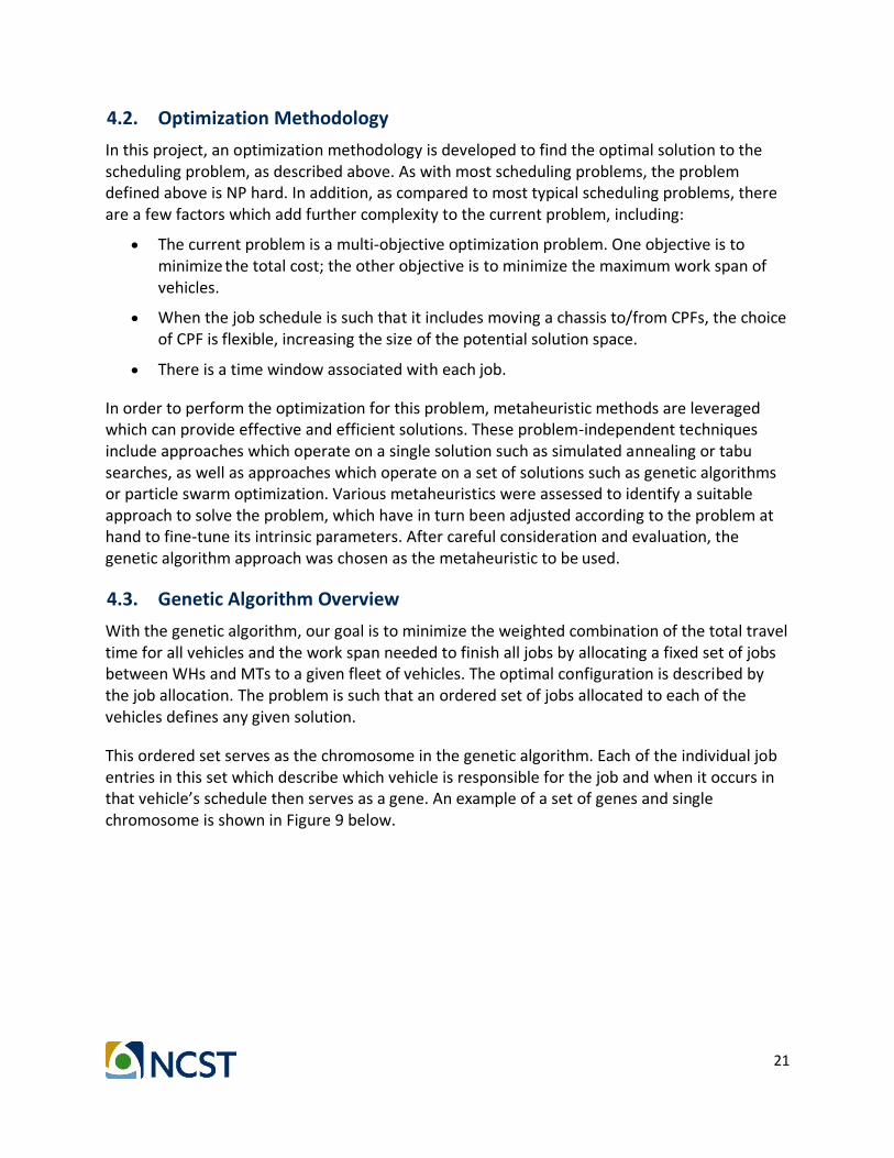
that each job is used exactly once, meeting the constraints of equations (4) and (5). The first vehicle’s schedule for the offspring is copied from that of parent 1, the second vehicle’s offspring is copied from that of parent 2, and then this alternating pattern is continued throughout the remainder of the rows. Redundant jobs are then removed and replaced sequentially through the offspring such that each job is used exactly once. An example of a crossover between two parents for N=60 and M=10 is shown in the figure below. The cases where a redundant job was replaced (such that the child’s schedule for a given vehicle does not exactly match one of the parents) are shown in red.
Figure 15. Crossover example
4.7. Mutation Function
Three different mutation functions were used with equal probability each time the mutation function was called. The first mutation function involved moving a job, whereas the second two mutation functions involved swapping of jobs rather than moving them. Note that for each of these three mutation functions the result could be moving / swapping jobs within a given vehicle’s schedule, or a moving / swapping jobs between two different vehicles’ schedules.
4.7.1. Mutation Function 1
In the first of the mutation functions, a single job was selected at random and moved into a random location. The job to be moved was selected by first randomly selecting one of the vehicle schedules with more than one job, and then randomly selecting among the jobs for that specific schedule. The destination was selected in a similar fashion by first selecting a vehicle schedule at random (this time allowing for any of the vehicle schedules to be selected regardless of jobs currently in the schedule), and then randomly selecting the location in the schedule into which the job would be inserted. An example of this algorithm is shown in Figure 16, where the job which is moved between parent and child is highlighted in red.

29
Figure 16. Mutation Function 1 Example
4.7.2. Mutation Function 2
In the first of the swapping mutation functions, two jobs were randomly selected and swapped with all jobs having equal likelihood of selection. An example of this algorithm is shown in Figure 17, where the jobs which are swapped between parent and child are highlighted in red.
Figure 17. Mutation Function 2 Example
30
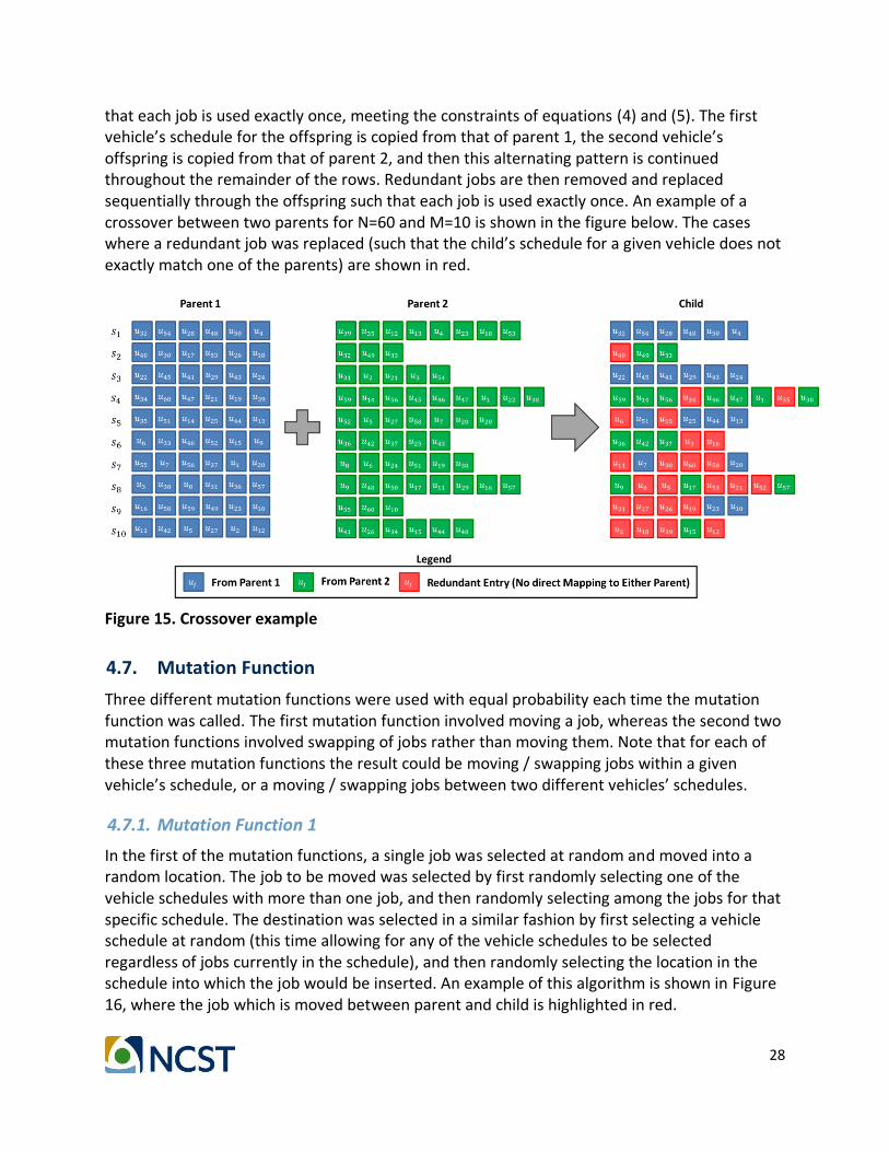
4.7.3. Mutation Function 3
In the final mutation algorithm, a swap was performed between the two jobs (𝑠𝑚,𝑖, and 𝑠𝑛,𝑗)
with the largest total job to job travel times according to equation (12) below.
max𝑚=1,…,𝑀,𝑛=1,…,𝑀
𝑡𝑗𝑜𝑏 (𝑠𝑚,𝑖−1, 𝑠𝑚,𝑖 , 𝑡𝑡𝑜𝑡(sm,i−1))
+ 𝑡𝑗𝑜𝑏 (𝑠𝑚,𝑖 , 𝑠𝑚,𝑖+1, 𝑡𝑡𝑜𝑡(sm,i))
+ 𝑡𝑗𝑜𝑏 (𝑠𝑛,𝑗−1, 𝑠𝑛,𝑗 , 𝑡𝑡𝑜𝑡(sn,j−1))
+ 𝑡𝑗𝑜𝑏(𝑠𝑛,𝑗 , 𝑠𝑛,𝑗+1, 𝑡𝑡𝑜𝑡(sn,j))
[𝑚𝑖] ≠ [
𝑛𝑗 ] (12)
An example of this algorithm is shown in Error! Reference source not found., where the jobs which are swapped between parent and child are highlighted in red. Note that the key difference between this mutation and the previous result from Mutation Function 2 is that 𝑠8,2
and 𝑠10,2 in Figure 17 were selected at random whereas 𝑠5,5 and 𝑠6,3 selected by Mutation Function 3 had the two largest values for job to job travel times in the parent chromosome as defined in equation (12) above.
Figure 18. Mutation Function 3 Example
4.8. Termination Function
The termination function used for the algorithm included a maximum number of total iterations which would be performed as well as a maximum number of iterations which would be performed in a row if the improvement in the cost was less than or equal to a fixed tolerance level.

31
5. Case Study Model Implementation
The analytical models and optimization methods described in Section 4 are applied in the case study to evaluate the potential CPF locations where the total cost and maximum work span for the trucking company will be minimized in a multi-objective cost function.
Real life simulation scenarios are developed using past, current and projected data from the LA/LB port area. The simulation scenarios are used to evaluate and compare two scenarios: base operations, and chassis and container movements with CPFs in the loop.
• Base Operations: The base operations replicate the current practices in the LA/LB port area. Here, the simulation experiments provide baseline data for total travel times and predicted work spans of vehicles for the modeled trucking company in the existing situation.
• CPFs for Chassis Operations: Simulation scenarios are developed and executed based on the results of the optimization procedure described above. The results of the various simulation scenarios with CPFs in the loop are compared to the base operations (when CPFs are not being used), and the improvements of using CPFs are quantified.
The case study uses the Marine Terminals in the POLB/POLA complex, one representative trucking company, a number of warehouses, and potential locations for chassis processing facilities in the vicinity of the ports. The selection methods for the TC, WHs and CPF locations are described in greater detail in the following sections.
A general overview of the local POLB and POLA area is shown in Figure 19, which indicates:
• The marine terminal locations at the POLB and POLA. The MTs are shown as the color- coded areas on the map.
• The TC used for the case study, which is shown as a yellow star on the map.
• The WHs used for the case study. The WHs are distributed in a wide area around the ports, and are shown as yellow dots on the map.
• The potential CPF locations used in the case study, which are distributed in a wide area around the ports and are shown as white pins on the map.

32
Figure 19. Node locations for the full model used in the simulation
5.1. Marine Terminals
The POLB and POLA have terminals which cover various categories of imports and exports such as automotive, dry bulk, break bulk liquid and containers. This study concentrates on import / export of containers and efficient retrieval and use of their associated chassis by truck. The container terminals at the POLB and POLA are listed in Table 2 and shown in Figure 20.
Table 2. Locations of POLB and POLA marine terminals used in the case study
MT ID Name Address 1 ITS (K-Line) Pier G E, Long Beach, CA 90802, USA
2 LBCT (OOCL) Pier F Ave, Long Beach, CA 90802, USA
3 Pacific Container Terminal (COSCO) Harbor Scenic Way, Long Beach, CA 90802, USA
4 SSA - Pier A Pier C St, Long Beach, CA 90802, USA 5 SSA (MSC, Zim, SMA/CGM) Pier A Way, Long Beach, CA 90802, USA
6 TTI (Hanjin) Hanjin Rd, Long Beach, CA 90802, USA
7 APM Terminals Pacific Navy Way Terminal Island, CA 90731
8 California United Terminals Navy Way, Terminal Island, CA 90731
9 China Shipping North America John S. Gibson Boulevard San Pedro, CA 90731 10 Eagle Marine Services Terminal Way, Los Angeles, CA 90731
11 Everport Terminal Services Terminal Island Way Terminal Island, CA 90731
12 TraPac, Inc South Neptune Avenue, Wilmington, CA 90744 13 Yang Ming Marine Transport John S. Gibson Boulevard, San Pedro, CA 90731
14 Yusen Terminal (Nyk Yusen) New Dock Street Terminal Island, CA 90731

33
Figure 20. POLB & POLA marine terminal locations
Loaded inbound (import) and outbound (export) quantities through the POLB and POLA for 2015 are included in Table 3.
Table 3. POLB and POLA import and export statistics for 2015
Loaded Import Loaded Export
TEU POLB 3,625,263 1,525,560
TEU POLA 4,159,462 1,786,913
TEU Total (Year) 7,784,725 3,312,473
TEU Total Avg (Day) 21,328 9,075
5.2. Trucking Companies
A representative trucking company was selected for this project. In order to select this TC, an initial list of TCs was created from an internet drayage directory which includes all companies operating within Los Angeles County. Since the location of the TCs is a critical variable for the optimization problem, all companies whose address was not included in the drayage directory were eliminated from the list. The final list contains all companies with known addresses using chassis. The trucking company to be used in this study, was then selected at random from this set.

34
5.3. Warehouses
In order to generate a representative set of warehouses covering the area of interest for the trucking company, a list similar to the list of addresses in Section 5.2 was used.
5.4. Central Processing Facilities
In the 2017 METRANS project by the principal investigators [8], potential CPF locations were identified by searching for vacant land within a 15-mile radius of the POLA and the POLB. In that study sixteen locations in the vicinity of the port were identified that could be potentially used as CPFs, and optimal CPF locations were identified based on the criterion of minimizing total travel time for all transactions undertaken by all the trucking companies noted above. The 16 CPF locations are noted in the table below. The table shows the street name and zip code of the potential CPF locations, but the exact street address numbers have been removed.
Table 4. Potential CPF locations for chassis storage
CPF ID Address
1 Golden Ave, Long Beach, CA 90806, USA
2 Via Oro Ave, Long Beach, CA 90810, USA
3 River Ave, Long Beach, CA 90810, USA
4 E 213th St, Carson, CA 90746, USA
5 E Del Amo Blvd, Carson, CA 90746, USA
6 Long Beach Blvd, Long Beach, CA 90805, USA
7 Long Beach Blvd, Long Beach, CA 90805, USA
8 S Sportsman Dr, Compton, CA 90221, USA
9 Atlantic Ave, Long Beach, CA 90805, USA
10 Alondra Blvd, Paramount, CA 90723, USA
11 Alondra Blvd, Paramount, CA 90723, USA
12 Torrance Blvd, Carson, CA 90745, USA
13 W Del Amo Blvd, Torrance, CA 90502, USA
14 W Del Amo Blvd, Torrance, CA 90502, USA
15 S Figueroa St, Wilmington, CA 90744, USA
16 Lomita Blvd, Carson, CA 90745, USA
The results of the previous study [8] showed that using the CPFs provided improvement (reduction) of the total travel time. The previous study also showed, during sensitivity analysis with respect to the number of CPFs employed for chassis exchange, that most of the improvement in the optimal solution was achieved when three CPFs were used. Employing more than three CPFs does not provide any significant improvement to the optimal solution. Therefore, only the three top CPF locations that were identified in the previous project were

35
used in the current case study. The three CPFs selected (CPF3, CPF6, and CPF15) are shown in Figure 21.
Figure 21. The three CPF locations selected for this study: CPF3, CPF6, and CPF15 The selected CPFs are marked with a blue pin.
5.5. Jobs
Jobs were selected randomly using the WH and MT locations noted previously by using the following assumptions:
• Import to Export ratio of 2 to 1
• Total number of jobs for the selected TC in one day is set to 60
• Wheeled vs. non-wheeled containers randomly selected with 50% probability of either for both WH and MT locations

36
• Minimum and maximum times for all jobs set to cover a 24-hour period, so that no constraints were placed on the time when each job could be performed
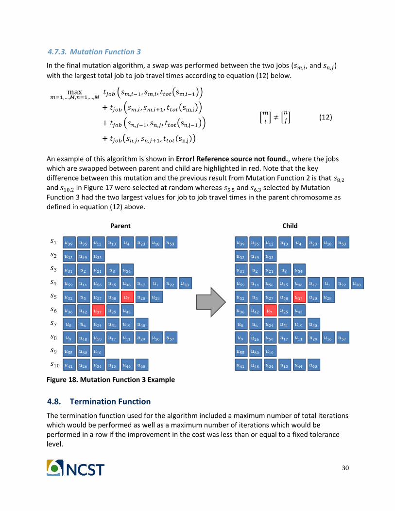
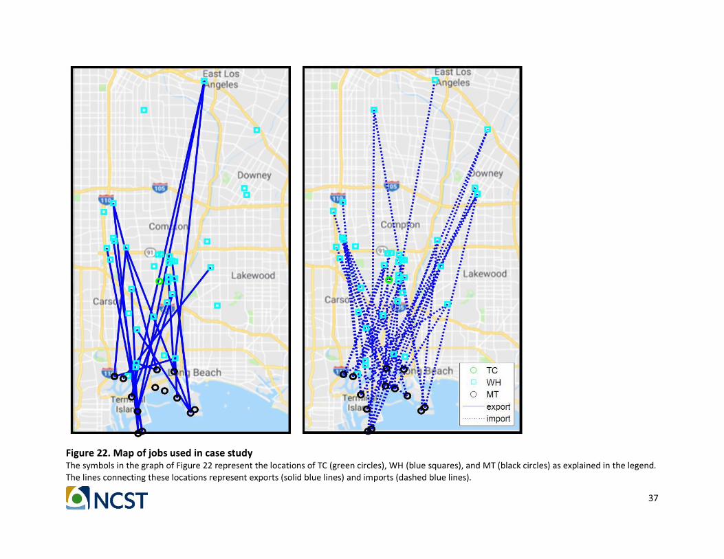
The jobs selected for this case study using this approach are shown in Figure 22, which represents a map of the area covered with WH nodes identified as cyan boxes, MTs identified as black circles, the TC identified as a green circle, the imports shown as blue dotted lines, and the exports shown as yellow solid lines.
37
Figure 22. Map of jobs used in case study
The symbols in the graph of Figure 22 represent the locations of TC (green circles), WH (blue squares), and MT (black circles) as explained in the legend. The lines connecting these locations represent exports (solid blue lines) and imports (dashed blue lines).

38
5.6. Travel Time Between Locations
The travel times between the TC and all of the WHs, CPFs and MTs were calculated using the Google Distance Matrix (GDM) Application Program Interface (API). In order to create a complete model of the area of interest to support the case study, time varying models covering a 24 hour period for a typical workday needed to be generated between all locations. For this particular case study this includes (1 + 𝐽 + 𝐾 + 𝐿)2 = (1 + 70 + 3 + 14)2 = 7,744 possible routes. In addition, the profiles of travel times from the GDM API are classified into two categories, using (a) pessimistic and (b) optimistic assumptions, as defined by the Google API. Therefore, in order to provide a time varying model for all possible routes matching a typical daily profile would result in 7,744 ∗ 2 ∗ 24/𝛿𝑡 individual queries, where 𝛿𝑡 is the time step of interest. For a time step of 5 minutes this will result in 4,460,544 queries to the Google API. However, the number of queries which can be made to the GDM API on a daily basis is limited, and the total number of queries above exceeds the GDM API limit by a large margin.
The main purpose for generating a time varying model for all possible routes is to make an assessment of the effectiveness of a complex approach, which considers the variation of traffic conditions throughout the day. With this goal in mind, and given that making the necessary 4,460,544 queries to GDM API is practically impossible, it was necessary to construct a suitable simplified model to represent the daily variations of travel times between any two arbitrary locations at a spacing of 5 minutes, using a limited set of queries.
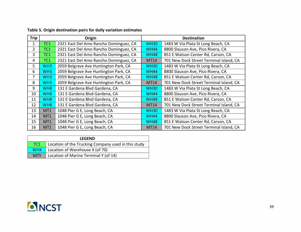
In order to generate the simplified model, a set of sixteen representative trips was considered initially, defined by sixteen origin/destination pairs as shown in Table 5. These sixteen characteristic trips were then queried for both optimistic and pessimistic times at a 5 minute spacing over a 24 hour period from midnight on Wednesday, July 25, 2018 to midnight Thursday, July 25, 2018, resulting in 16*2*288 = 9,216 queries. The locations selected are listed in Table 5 and then shown on Figure 23. In Table 5, locations are color coded by the location type where the TC is highlighted in Green, the WHs in cyan, and the MTs in grey. In Figure 23, the origins are shown in green, and the destinations in red, with all other nodes shown as x’s.
39
Table 5. Origin destination pairs for daily variation estimates
Trip Origin Destination 1 TC1 2321 East Del Amo Rancho Dominguez, CA WH30 1483 W Via Plata St Long Beach, CA 2 TC1 2321 East Del Amo Rancho Dominguez, CA WH44 8800 Slauson Ave, Pico Rivera, CA 3 TC1 2321 East Del Amo Rancho Dominguez, CA WH48 851 E Watson Center Rd, Carson, CA
4 TC1 2321 East Del Amo Rancho Dominguez, CA MT14 701 New Dock Street Terminal Island, CA 5 WH3 2059 Belgrave Ave Huntington Park, CA WH30 1483 W Via Plata St Long Beach, CA 6 WH3 2059 Belgrave Ave Huntington Park, CA WH44 8800 Slauson Ave, Pico Rivera, CA 7 WH3 2059 Belgrave Ave Huntington Park, CA WH48 851 E Watson Center Rd, Carson, CA
8 WH3 2059 Belgrave Ave Huntington Park, CA MT14 701 New Dock Street Terminal Island, CA 9 WH8 131 E Gardena Blvd Gardena, CA WH30 1483 W Via Plata St Long Beach, CA
10 WH8 131 E Gardena Blvd Gardena, CA WH44 8800 Slauson Ave, Pico Rivera, CA 11 WH8 131 E Gardena Blvd Gardena, CA WH48 851 E Watson Center Rd, Carson, CA 12 WH8 131 E Gardena Blvd Gardena, CA MT14 701 New Dock Street Terminal Island, CA 13 MT1 1048 Pier G E, Long Beach, CA WH30 1483 W Via Plata St Long Beach, CA 14 MT1 1048 Pier G E, Long Beach, CA WH44 8800 Slauson Ave, Pico Rivera, CA 15 MT1 1048 Pier G E, Long Beach, CA WH48 851 E Watson Center Rd, Carson, CA 16 MT1 1048 Pier G E, Long Beach, CA MT14 701 New Dock Street Terminal Island, CA
LEGEND TC1 Location of the Trucking Company used in this study
WHX Location of Warehouse X (of 70)
MTY Location of Marine Terminal Y (of 14)

40
Figure 23. Map of jobs used in daily traffic variation model The symbols in the graph of Figure 23 represent the origin and destination points as explained in the legend, based on the locations given in Table 5.
For the sixteen trips noted above, optimistic and pessimistic travel times were calculated at a 5-minute spacing.
One example of the driving paths between an origin/destination pair is shown in Figure 24. The example origin/destination pair corresponds to the fourth row (Trip 4) of Table 5, between trucking company TC1 (origin) and marine terminal MT14 (destination).
In this query the Google API was asked to provide time travel estimates between TC1 and MT14 at peak traffic time. The GDM API suggests three alternate paths and a range of travel time

41
estimates for each alternative path. For example, it is seen that the optimistic travel time for the path highlighted in blue is 20 minutes, whereas the pessimistic travel time estimate for the blue path is 40 minutes. Note that the Google API only provides estimates for typical passenger car routing, and there may be times when trucks cannot follow the same routes that are available to typical passenger car traffic. In addition, one can see that, at this peak travel time, the optimum route suggested by the Google API (blue path) actually shows a slightly longer pessimistic travel time estimate than one of the other alternative paths (40 min vs. 35 min). This is worth noting only for the fact that the data as delivered for pessimistic and optimistic travel times may have some inherent noise due to the algorithms and routing approaches intrinsic to the Google routing. Using the 5-minute spacing, the graphs in Figure 25 through Figure 32 show the daily profiles of travel time estimates between the 16 origin and destination pairs used in the case study.

42
Figure 24. Peak predicted travel time Minimum time route is highlighted in blue.
43
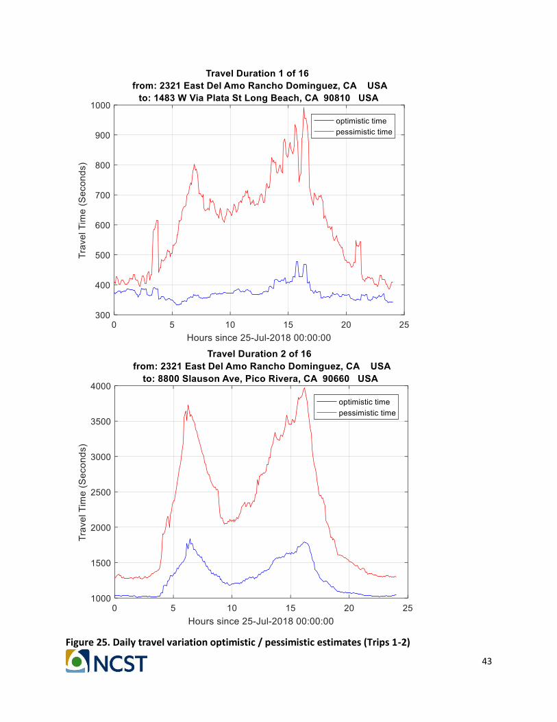
Figure 25. Daily travel variation optimistic / pessimistic estimates (Trips 1-2)

44
Figure 26. Daily travel variation optimistic / pessimistic estimates (Trips 3-4)

45
Figure 27. Daily travel variation optimistic / pessimistic estimates (Trips 5-6)
46
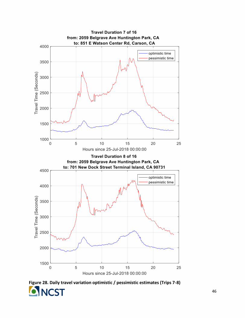
Figure 28. Daily travel variation optimistic / pessimistic estimates (Trips 7-8)
47
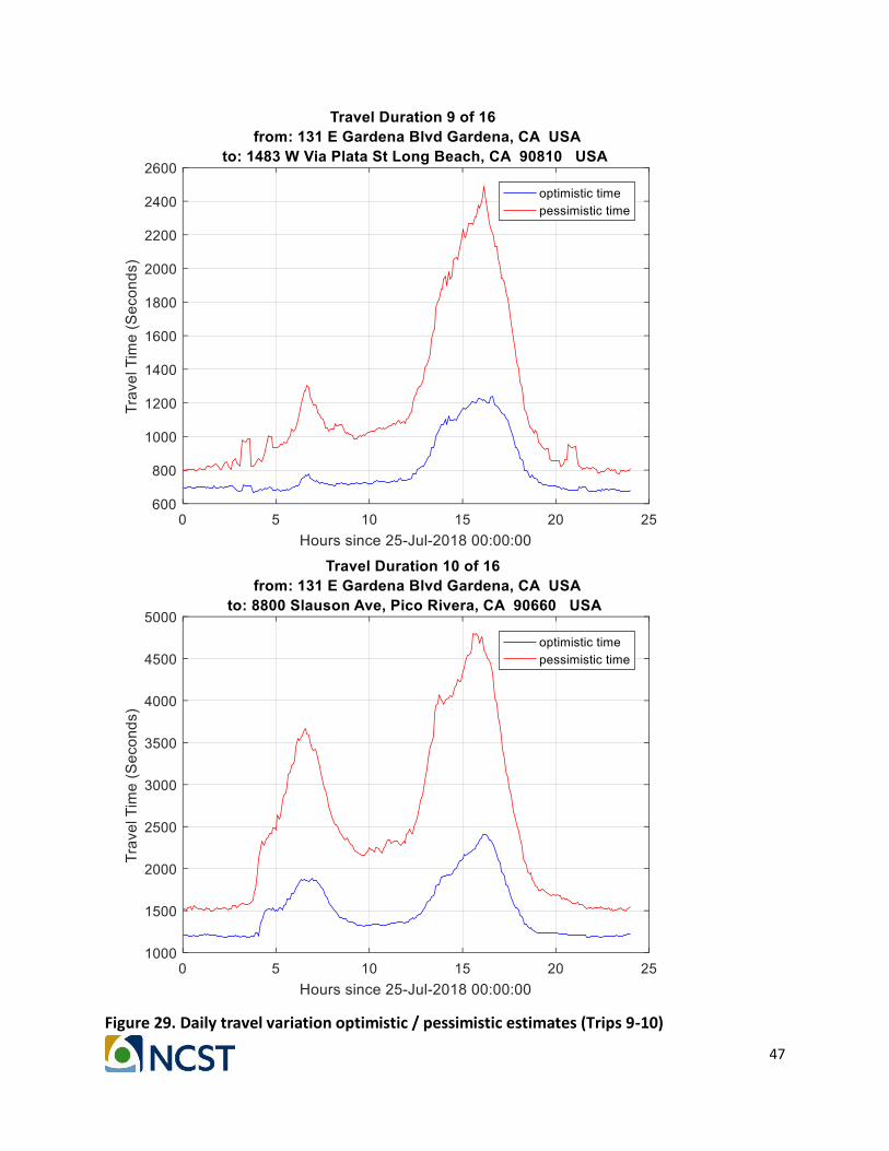
Figure 29. Daily travel variation optimistic / pessimistic estimates (Trips 9-10)

48
Figure 30. Daily travel variation optimistic / pessimistic estimates (Trips 11-12)
49
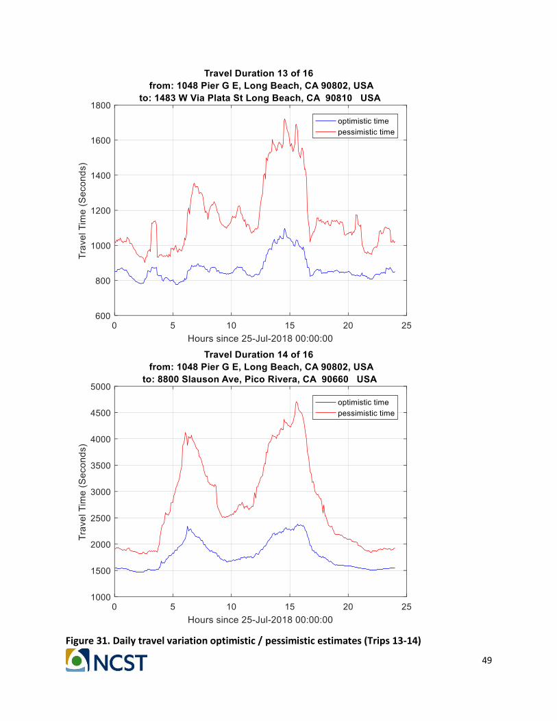
Figure 31. Daily travel variation optimistic / pessimistic estimates (Trips 13-14)

50
Figure 32. Daily travel variation optimistic / pessimistic estimates (Trips 15-16)

51
Figure 33 and Figure 34 show a summary of the optimistic and pessimistic travel time estimates for all 16 trips used in the case study. The black trace in Figure 33 provides an average optimistic travel time estimate over all 16 trips. Similarly, the black trace in Figure 34 provides an average pessimistic travel time estimate over all 16 trips. The traces in Figure 35 have been constructed to show the average travel time (i.e. the mid-point between the optimistic and the pessimistic estimates) for each of the 16 trips. The black trace in Figure 35 provides an average of the average travel time estimate over all 16 trips. In general, it can be seen that there is a similar pattern across most of the trips in which the travel time profiles have peaks during rush hour periods, typically from 5:00 to 7:00 a.m., and from 2:00 to 6:00 p.m. It is noted that the peaks are much more pronounced in the pessimistic models than they are in the optimistic models.
Figure 33. Optimistic travel time estimates

52
Figure 34. Pessimistic travel time estimates
Figure 35. Average travel time estimates
53
The next phase in generating the simplified model is the construction of a simple function 𝑔 which can be used by the genetic algorithm, whenever a coarse prediction of the time varying traffic conditions is needed. For this purpose, first a total of 7,744 queries were made to GDM API, to obtain the travel times at midnight for all 7,744 possible routes between origins and destinations used in the case study, as described at the beginning of section Error! Reference source not found.. Next the average of the average travel time profiles was obtained, which is plotted as the solid black trace in Error! Reference source not found., and is denoted by �̅� in the sequel. Finally, the function 𝑔 was constructed as shown below. Function 𝑔 is used to
provide coarse estimates of the travel time �̂�𝑛𝑜𝑑𝑒(𝑥𝑖 , 𝑥𝑗 , 𝑡𝑘) between two arbitrary nodes 𝑥𝑖
and 𝑥𝑗 at time 𝑡𝑘. Given a pair of nodes 𝑥𝑖 , 𝑥𝑗 the input to the function 𝑔 will be the average
travel time at midnight between 𝑥𝑖 and 𝑥𝑗 as explained above, denoted by 𝑡𝑛𝑜𝑑𝑒(𝑥𝑖 , xj, 0) in
the sequel. Using this 𝑡𝑛𝑜𝑑𝑒(𝑥𝑖, xj, 0) and the complete set of data for travel time estimates
throughout the day that were generated by the sixteen representative trips, a least squares model for the function 𝑔 was created.
�̂�𝑛𝑜𝑑𝑒(𝑥𝑖 , xj, 𝑡𝑘) = 𝑔(𝑡𝑛𝑜𝑑𝑒(𝑥𝑖 , xj, 0), 𝑡𝑘) (13)
The function, 𝑔, was modeled to be of the form
𝑔(𝑡𝑛𝑜𝑑𝑒(𝑥𝑖, xj, 0), 𝛿𝑡 ∗ 𝑗) = 𝛼 + 𝛽𝑡𝑛𝑜𝑑𝑒(𝑥𝑖, xj, 0) + (𝛾 + 𝜌𝑡𝑛𝑜𝑑𝑒(𝑥𝑖 , xj, 0))�̅�𝑗
𝑗 = {0,… , 𝑛}
(14)
where 𝑛 = 24 ∗ 3600/𝛿𝑡 (15)
�̅�𝑗 =∑ 𝑦𝑘,𝑗
16𝑘=1
16 𝑗 = {0,… , 𝑛} (16)
𝑦𝑘,𝑗 ≡ The typical duration from the GDM API for trip k at time sample i (17) 𝑘 = {1,… ,16} 𝑗 = {0,… , 𝑛}
and 𝛼, 𝛽, 𝛾, and 𝜌 are model parameters to be determined
The step-size 𝛿𝑡 of the measurements is represented in seconds. For the data above all
values were recorded at a 5 minute (300 second) spacing giving 𝑛 = 24 ∗3600
300= 288.
In order to find the best estimates for model parameters 𝛼, 𝛽, 𝛾, and 𝜌 a least squares fit was performed, solving equation (18) below for the best estimate, in a least squares sense, of x given by �̂� = (𝐴𝑇𝐴)−1𝐴𝑇𝑦. The fitted values were then used in equation Error! Reference source not found. and applied to each of the 16 representative trip values at midnight to provide a comparison between the route specific detailed estimates and those based upon the least squares fit and the average data in equation Error! Reference source not found..
The comparisons between the simplified model and the individual data sets are plotted in Error! Reference source not found. through Error! Reference source not found..

54
𝑦 = 𝐴𝑥 (18)
where 𝑥 = [
𝛼𝛽𝛾𝜌
] (19)
𝑦 = [
𝑦1
⋮𝑦16
] (20)
𝑦𝑘 = [
𝑦𝑘,0
⋮𝑦𝑘,𝑛
] (21)
�̅� = [�̅�0
⋮�̅�𝑛
] (22)
𝐴 =
[ 1𝑛 1𝑛
⋮1𝑛
1𝑛
𝑦1,01𝑛
𝑦2,01𝑛
⋮𝑦15,01𝑛
𝑦16,01𝑛
�̅��̅�⋮�̅��̅�
𝑦1,0�̅�
𝑦2,0�̅�
⋮𝑦15,0�̅�
𝑦16,0�̅�]
(23)

55
Figure 36. Daily travel variation vs. least square fit (1-2)
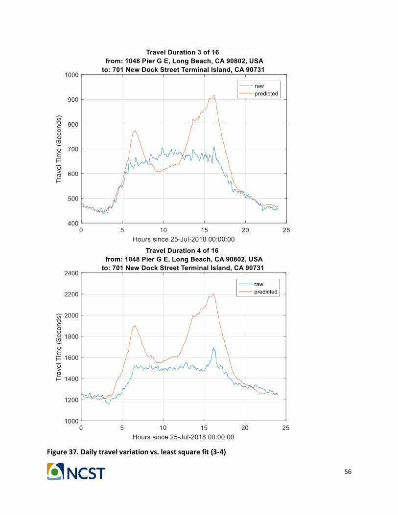
56
Figure 37. Daily travel variation vs. least square fit (3-4)

57
Figure 38. Daily travel variation vs. least square fit (5-6)

58
Figure 39. Daily travel variation vs. least square fit (7-8)

59
Figure 40. Daily travel variation vs. least square fit (9-10)

60
Figure 41. Daily travel variation vs. least square fit (11-12)

61
Figure 42. Daily travel variation vs. least square fit (13-14)

62
Figure 43. Daily travel variation vs. least square fit (15-16)
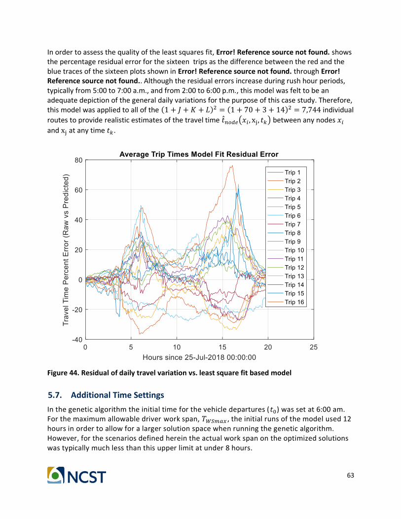
63
In order to assess the quality of the least squares fit, Error! Reference source not found. shows the percentage residual error for the sixteen trips as the difference between the red and the blue traces of the sixteen plots shown in Error! Reference source not found. through Error! Reference source not found.. Although the residual errors increase during rush hour periods, typically from 5:00 to 7:00 a.m., and from 2:00 to 6:00 p.m., this model was felt to be an adequate depiction of the general daily variations for the purpose of this case study. Therefore, this model was applied to all of the (1 + 𝐽 + 𝐾 + 𝐿)2 = (1 + 70 + 3 + 14)2 = 7,744 individual
routes to provide realistic estimates of the travel time �̂�𝑛𝑜𝑑𝑒(𝑥𝑖 , xj, 𝑡𝑘) between any nodes 𝑥𝑖
and xj at any time 𝑡𝑘.
Figure 44. Residual of daily travel variation vs. least square fit based model
5.7. Additional Time Settings
In the genetic algorithm the initial time for the vehicle departures (𝑡0) was set at 6:00 am. For the maximum allowable driver work span, 𝑇𝑊𝑆𝑚𝑎𝑥 , the initial runs of the model used 12 hours in order to allow for a larger solution space when running the genetic algorithm. However, for the scenarios defined herein the actual work span on the optimized solutions was typically much less than this upper limit at under 8 hours.
64
In order to account for the additional difficulty of picking up and dropping off grounded containers as compared to wheeled containers, the time to pick up or drop-off wheeled containers (𝑇𝑤ℎ) was set at 5 minutes whereas the time to pick up or drop-off grounded containers (𝑇𝑔𝑛𝑑 ) was set at 15 minutes.
Lastly, it is assumed that there will be an inherent advantage in using the CPFs over the MTs for chassis retrieval and drop-off. This is due to the CPF’s ability to maintain road-worthy chassis which are already unstacked and available to support chassis retrieval as well as the CPF’s larger space allocation to allow for chassis to be detached from the bobtail, so that truck drivers can quickly move on from the facility and onto their next job after drop-off. These improvements were modeled by including reduced chassis retrieval and drop-off times at CPFs as compared to those at MTs. The difference between the processing time at MTs and that at CPFs, is referred to as “Additional Processing Time” and denoted by 𝑃. This parameter 𝑃, defined in equation (24), provides a measure of the relative advantage of routing a transaction through a CPF over routing the transaction directly to the MT. Previous results [8] have shown that the parameter 𝑃 is an important factor in evaluating the effectiveness of the use of CPFs.
𝑃 = 𝑃(𝑥) − 𝑃(𝑦) 𝑥 𝜖 ℳ𝒯
𝑦 𝜖 𝒞𝒫ℱ (24)
Based on similar considerations as in [8], the processing time for chassis retrieval / drop-off, 𝑃(𝑦), was set at 5 minutes for 𝑦 𝜖 𝒞𝒫ℱ. The processing time 𝑃(𝑥), was set at either 15 or 25 minutes for 𝑥 𝜖 ℳ𝒯 depending upon the specific scenario being evaluated. The two values selected for MT processing times result in 𝑃 = 600 and 𝑃 = 1200 seconds of “Additional Processing Time” respectively.
5.8. Optimization and Genetic Algorithm Specific Settings
For all case studies and sensitivity analyses in Section Error! Reference source not found. through Section Error! Reference source not found., the cost of each schedule, 𝐶(sm) of equation (11), was assumed to be equal to the travel time to complete vehicle 𝑣𝑚’s schedule 𝑇(sm). This results in a simplified objective function, equation (1), of the form:
min ∑ 𝑇(𝑠𝑚)
𝑀
𝑚=1
+ 𝜇 max𝑚=1,…,𝑀
𝑇(𝑠𝑚) (25)
In this form, the objective function minimizes the weighted sum of the total travel time needed to complete all vehicles’ schedules, ∑ 𝑇(𝑠𝑚)𝑀
𝑚=1 , and the maximum work span across all of the vehicles’ schedules, max
𝑚=1,…,𝑀𝑇(𝑠𝑚). As 𝜇 increases, the objective function will force more
uniformity across the vehicles’ schedules, so that all vehicles have approximately the same work span. A sensitivity analysis was performed as a function of 𝜇 in Section Error! Reference source not found.. In that analysis, a reasonable value which maintained uniformity across
65
vehicles’ schedules for the given job set was identified as 𝜇 = 1, which was in turn used as the nominal setting in the other case studies.
In addition, the following configuration was used for the genetic algorithm.
• The population was set at 60
• 500 generations were run unless a stall limit of no improvement for 200 generations in a row was reached
• 10 of each subsequent generation were generated by passing on the best “elite” solutions from the previous generation as is
• 25 of each subsequent generation were created using the crossover function
• 25 of each subsequent generation were created using the mutation function
The genetic algorithm parameters, including population, number of total generations and stall generations as well as the composition of each generation by direct passing of fittest parents, crossover, and mutation were arrived at through early experimentation when developing the genetic algorithm. During this experimentation values in the following range were evaluated:
• Population Size: 60-1000
• Elite Count: 1-25
• Number of Generations: 500-1500
• Stall Limit: 200-600
The population size, number of generations, and stall limit all showed approximately linear increases in computational time as the values increased, for less than 1% improvement in the overall result.
Increasing the elite count showed a reduction in overall computational time, however the value of 10 was selected as an upper limit, as increasing the elite count too high came with the risk of allowing the model to become trapped at a local optimum. For the given case study parameters, the values above were found to provide good solutions in several minutes where no significant improvements (i.e. greater than 1%) were seen with increased generations or populations sizes.
66
6. Case Study Simulation Results
This section presents the results of several simulation scenarios for the case study, based on the optimization formulation and case study model implementation described previously.
6.1. Genetic Algorithm Evaluation
A typical genetic algorithm output is shown in Figure 45 and Figure 46. Figure 45 shows one of the ten vehicle schedules, namely vehicle 𝑉𝑉2, and Figure 46 shows the complete chromosome with all vehicle schedules. These outputs were generated for 𝑀𝑀 = 10 vehicles for a particular day, when they have to complete 𝑁𝑁 = 60 jobs. In the figures:
• each solid blue line represents a specific job
• each dotted line indicates an additional move to CPF or MT in order to perform a chassis exchange or a relocation between jobs
• numbers next to each node indicate the order of arrival between nodes
• a green circle indicates the TC
• red circles indicate CPFs
• cyan squares indicate the WHs
• black circles indicate the MTs.

67
Figure 45. Example of truck schedule (𝒔𝟐) used in the case study The schedule was generated by the genetic algorithm for vehicle 𝑽𝟐 , with M=10 and N=60

68
Figure 46. Genetic algorithm chromosome example output for M=10 and N=60
During the initial genetic algorithm assessment, various settings were evaluated before converging on the settings defined in Sections 4.4 and Section 5.8. One of these early improvements to the algorithm was the addition of the nearest neighbor solution to the initial population. In the original version of the genetic algorithm the initial population was created by using only random sequencing and allocations of the jobs to the vehicles. Early in the development the initial population was updated to include a nearest neighbor solution in which each of the 10 vehicles’ routes performed sequential nearest neighbor routing (See section 4.4 for additional details). The improvement in the conversion of the
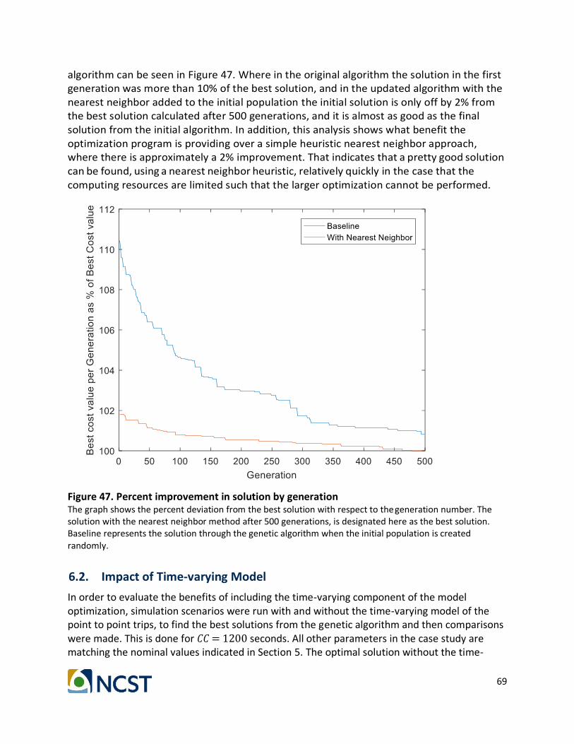
69
algorithm can be seen in Figure 47. Where in the original algorithm the solution in the first generation was more than 10% of the best solution, and in the updated algorithm with the nearest neighbor added to the initial population the initial solution is only off by 2% from the best solution calculated after 500 generations, and it is almost as good as the final solution from the initial algorithm. In addition, this analysis shows what benefit the optimization program is providing over a simple heuristic nearest neighbor approach, where there is approximately a 2% improvement. That indicates that a pretty good solution can be found, using a nearest neighbor heuristic, relatively quickly in the case that the computing resources are limited such that the larger optimization cannot be performed.
Figure 47. Percent improvement in solution by generation The graph shows the percent deviation from the best solution with respect to the generation number. The solution with the nearest neighbor method after 500 generations, is designated here as the best solution. Baseline represents the solution through the genetic algorithm when the initial population is created randomly.
6.2. Impact of Time-varying Model
In order to evaluate the benefits of including the time-varying component of the model optimization, simulation scenarios were run with and without the time-varying model of the point to point trips, to find the best solutions from the genetic algorithm and then comparisons were made. This is done for 𝐶𝐶 = 1200 seconds. All other parameters in the case study are matching the nominal values indicated in Section 5. The optimal solution without the time-

70
varying model assumed a constant travel time for a given trip, without any variations during the day. The optimization process was then repeated with the time-varying model to determine the optimal schedules when the point-to-point durations are modeled to vary throughout the day. The cost of the two resultant optimized schedules was then compared, using the cost function with time variation. The result was that the version optimized for the time-varying case showed ~1% improvement over that which was optimized for the static case. For this specific case it indicates a small potential benefit in including the time-varying model during the optimization process.
6.3. Impact of CPFs
In order to assess the impact of the use of CPFs, several cases were run. These cases were run for 𝐶𝐶 = 600 seconds and 𝐶𝐶 = 1200 seconds, over a range of a number of jobs from 𝑁𝑁 = 10 to 𝑁𝑁 = 60.
• Cases with CPFs. When CPFs are present and can be utilized (designated as cases “with CPFs” on the plots), chassis exchanges were allowed to occur in both CPFs and MTs. The average processing time for chassis at a CPF was set at 300 seconds. The average processing time at a MT was set at either 900 seconds (when the parameter 𝐶𝐶 = 600 seconds), or at 1500 seconds (when the parameter 𝐶𝐶 = 1200 seconds).
• Cases without CPFs. When CPFs are not available (designated as cases “without CPFs” on the plots), all necessary chassis exchanges are forced to occur at one of the MTs, The same average processing time as before of either 900 seconds or 1500 seconds has been used.
In addition, these cases were run for two scenarios to allow for better comparison to the previous work reported in [8]. The main factors in the two scenarios are the attributes of successive jobs, in particular attribute (iv) of Job𝑘, and attribute (iii) of Job𝑘+1, as defined in Section Error! Reference source not found..
• Scenario 1. In this scenario, if attribute (iv) of Job𝑘 is the same as attribute (iii) of Job𝑘+1, i.e., if the container configuration at the destination point of Job𝑘 is identical to the container configuration at the origin point of Job𝑘+1, then the truck driver does not need to travel to a CPF or to a MT to pickup or dropoff a container.
• As an example, for the jobs defined in Table 5 and represented in Figure 7 it can be seen that:
o Attribute (iv) of Job1 shows that the container at the destination is left in a grounded configuration, hence the truck departs the destination point of Job1 carrying a chassis, and arrives at the origin point of Job2 with a chassis.
o Attribute (iii) of Job2 shows that the container at the origin point of Job2 is grounded, hence the truck will load the container on the chassis. The truck does not need to perform a drop-off or pick-up chassis operation while transitioning from Job1 to Job2.

71
o Attribute (iv) of Job2 shows that the container will be left at the destination point of Job2 in a wheeled configuration, hence the truck leaves the destination point of Job2 as a bobtail.
o Attribute (iii) of Job3 shows that the container at the origin point of Job3 is grounded, hence the truck after completing Job2 will need to pick up a chassis before starting Job3. In this particular example, the truck will pick up a chassis at CPF𝑘 as shown in Figure 7.
• Scenario 2. In this scenario a chassis operation (pick-up or drop-off) is forced to occur between jobs, regardless of container configuration. The reason for this scenario is to provide a better comparison of the current study to the previous project [8], where every transaction was grounded and required the truck driver to stop at a CPF or MT in order to complete a job. Consequently, Scenario 1 above, results in a smaller number of chassis transactions than what was modeled and reported in [8]. Scenario 2 will provide a limiting upper bound for what might occur in the real world when there are additional limitations of chassis usage, and there are job to job differences in chassis configuration needs (i.e., not all jobs are 40 FT containers of the same type).
The results for Scenario 1 are shown in Figure 48 through Figure 50. The results for Scenario 2 are shown in Figure 51 through Figure 53.
Scenario 1 allows for direct routing between origin and destination (i.e. a CPF is used only if the container configuration at origin does not match the container configuration at destination). In Figure 48 the greatest improvement for the cost function due to the use of CPFs is seen to occur for small ratios of jobs to vehicles. When the number of jobs is small, the improvement ranges from about 2% (when 𝐶𝐶 = 600 sec) to about 6% (when 𝐶𝐶 = 1200 sec). For large ratios of jobs to vehicles there is only a small benefit at ~1% for 60 jobs (allocated between 10 vehicles). Figure 49 and Figure 50 show a qualitative representation of the relative difference between the solutions with small and large ratios of jobs to vehicles. Note that in the figures any time a CPF is being used, it is because it is saving time as compared to the use of a MT for the chassis exchange. Therefore, the greater number of paths connected to CPFs, is a qualitative indication of the potential for additional reductions in total travel time as compared to the case where CPFs are not available.
Scenario 2 forces a chassis operation to occur between jobs, regardless of container configuration. The chassis operation may occur at a CPF or at a MT. Figure 51 shows an improvement of 5% to 10% when the number of jobs is small, and an improvement of 8% to 13% when the number of jobs is large, under scenario 2. It is noted that this analysis is from the point of view of a single trucking company (i.e. at the operational level), but the observed behavior is similar to what was observed during the analysis at the strategic level in [8] which showed 6% - 20% improvements in total travel time for the overall network.
Note that there is not a direct comparison here as a different TC set is being used and the original study used total travel time rather than a weighted combination of total travel time and

72
work span. The current results imply that for typical cases where the number of jobs is much larger than the number of vehicles, the greatest benefit from CPFs is in the cases where there are at least some significant job to job differences in container configuration. This implies a slightly different take on some of the conclusions which came out of the original study [8]. These results suggest that it would be important to include a variety of chassis types at the CPFs, and consider the inclusion of different types of chassis in the modeling process, as a topic for future research.
Figure 48. Scenario 1: Total cost improvement due to use of CPFs In Scenario 1, a CPF is used only if the container configuration at origin does not match the container configuration at the destination of a job. The percent improvement is computed in comparison to the case when no CPFs are used.

73
Figure 49. Scenario 1: Solution (a) without CPFs and (b) with CPFs, N=10, P=1200 seconds

74
Figure 50. Scenario 1: Solution (a) without CPFs and (b) with CPFs, N=60, P=1200 seconds

75
Figure 51. Scenario 2: Total cost improvement due to use of CPFs In scenario 2, the truck always uses a CPF when transitioning from one job to the next. The improvement is computed in comparison to the case when no CPFs are used.
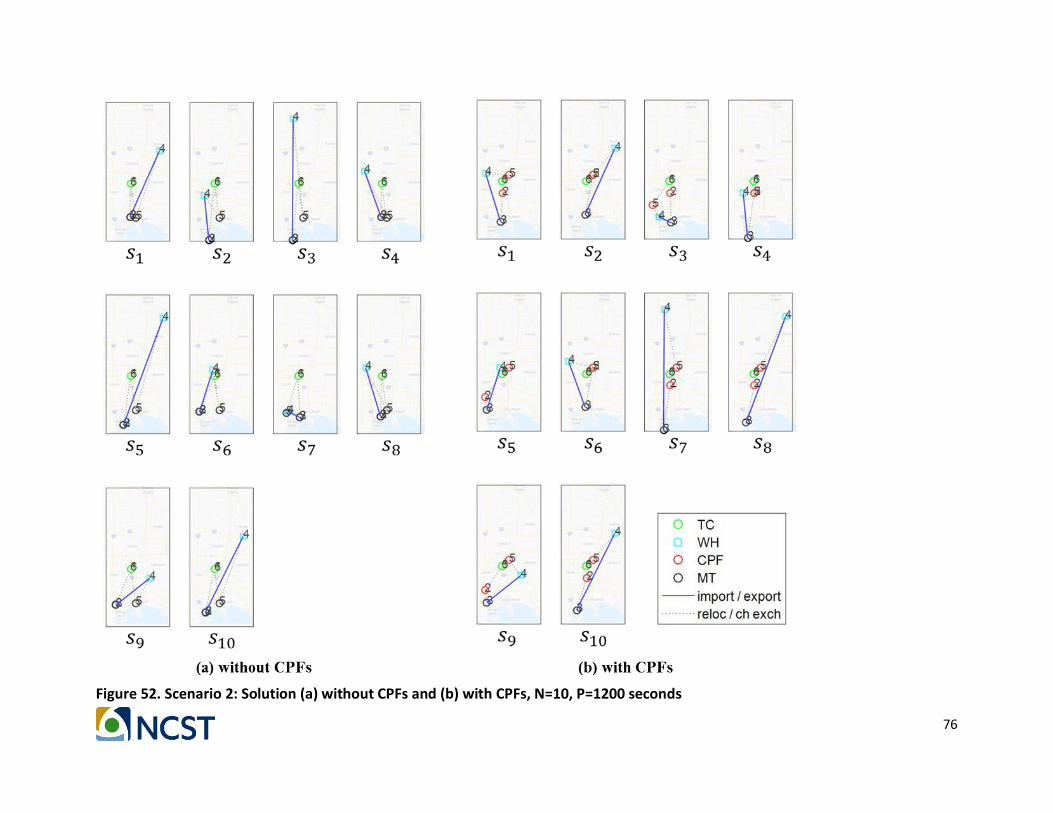
76
Figure 52. Scenario 2: Solution (a) without CPFs and (b) with CPFs, N=10, P=1200 seconds
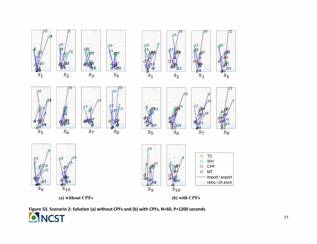
77
Figure 53. Scenario 2: Solution (a) without CPFs and (b) with CPFs, N=60, P=1200 seconds

78
6.4. Sensitivity Analysis for 𝝁
A sensitivity analysis was performed for varying values of the weight 𝜇 in the objective function. In equation (25) the objective function minimizes the weighted sum of the total travel time needed to complete all vehicles’ schedules, ∑ 𝑇(𝑠𝑚)𝑀
𝑚=1 , and the maximum work span across all of the vehicles’ schedules, max
𝑚=1,…,𝑀𝑇(𝑠𝑚). As the weight 𝜇 increases, it is anticipated that the
objective function will force more uniformity across the vehicles’ schedules such that all vehicles will have approximately the same work span. This sensitivity analysis was performed using values of 𝜇 between 0 and 1, for 𝑃 = 1200 seconds and for a total number of jobs 𝑁 =60.
The total travel time with respect to the weight µ is shown in Figure 54.The maximum work span max
𝑚=1,…,𝑀𝑇(𝑠𝑚) and the minimum work span min
𝑚=1,…,𝑀𝑇(𝑠𝑚) are shown in Figure 55.
For 𝜇 = 0, no optimization is performed with respect to the maximum work span, so that as seen in Figure 55, there is a large variation between the minimum and maximum work span of the drivers. The total travel time, however, is at its minimum when 𝜇 = 0.
As 𝜇 increases the maximum and minimum work spans converge so that the drivers are more equally loaded as seen in Figure 55, and there is a slight increase observed in the total travel time (by up to ~1%), shown in Figure 54. Depending upon the policies in place for driver pay (e.g. minimum hours to be worked per day, cost of overtime pay, etc.), 𝜇 could be tuned to allow for optimization of the overall cost to the trucking company. As the variation between the maximum and minimum work spans converges to a reasonable value of approximately 1 hour for 𝜇 = 1, this value of 𝜇 was used for the nominal setting in the other case studies.

79
Figure 54. Total travel time vs. 𝝁 The parameter µ is the weight used in the objective function as defined in equation (25)
Figure 55. Work span vs. 𝝁 The parameter µ is the weight used in the objective function as defined in equation (25).
80
7. Summary
This study examines the scheduling of chassis and container movements at the operational level, from the point of view of individual trucking companies, when Chassis Processing Facilities (CPFs) are available for use, in the vicinity of a container port within a major metropolitan area. An optimization methodology is developed, which minimizes the travel time for the fleet of trucks used by the trucking company, and at the same time tries to minimize the variations in work load among individual drivers during the day. The optimal solution is obtained through the application of a genetic algorithm, developed specifically for this purpose. Time-varying dynamic models for the movements of chassis and containers are developed to be used in the optimization process. The effectiveness of the methodology is evaluated through a case study, which is focusing on the Los Angeles/Long Beach port complex and surrounding areas. A location for the trucking company is chosen, and the company’s fleet of trucks is assigned a series of container movements to be completed during the day. Two scenarios are considered in the simulations: (1) when the truck does not have to pick up or drop off a chassis from one job to the next; and (2) when the truck must pick up or drop off a chassis from the previous job to the next. Simulation results show that the optimal solution obtained through the genetic algorithm provides improvements to the objective function when CPFs are used over the case when no CPFs are available. The improvements are modest (up to 6%) for cases where scenario (1) is applicable, or more significant (up to 13%) in cases when scenario (2) is applicable.

81
8. References
[1] "The World Bank," 2018. [Online]. Available: http://www.worldbank.org/. [Accessed 15 May 2017].
[2] "Port of Los Angeles Statistics," 2017. [Online]. Available: https://www.portoflosangeles.org/Stats/stats_2017.html.
[3] "Port of Long Beach Statistics," 2017. [Online]. Available: http://www.polb.com/economics/stats/yearly_teus.asp.
[4] The Tioga Group, "Empty Ocean Logistics Study," Technical Report, Submitted to the Gateway Cities Council of Governments, 2002.
[5] G. Konstantzos, E. Saharidis and G. Loizidou, "Development of a model for assessing Greenhouse Gas (GHG) emissions from terminal and drayage operations," Operational Research, vol. 17, no. 3, pp. 807-819, 2017.
[6] O. Jabali, T. Woensel and A. De Kok, "Analysis of Travel Times and CO 2 Emissions in Time‐Dependent Vehicle Routing," Production and Operations Management, vol. 21, no. 6, pp. 1060-1074, 2012.
[7] I. The TIOGA Group, U. A. C. f. T. Research and S. D. o. C. &. E. Engineering, "NCFRP Report 11: Truck Drayage Productivity Guide," Transportation Research Board, 2011.
[8] A. Chassiakos, H. Jula, T. Vanderbeek, M. Shellhammer and S. An, "Analysis and Optimization Methods for Centralized Processing of Chassis," February 2017. [Online]. Available: https://metrans.org/.
[9] T. Vanderbeek, M. Shellhammer, S. An, H. Jula and A. Chassiakos, "Analysis and optimization of chassis movements in transportation networks with centralized processing of chassis facilities," in National Urban Freight Conference, Long Beach, CA, 2017.
[10] T. O'Brien, T. Reeb and A. Kunitsa, "Mitigating Urban Freight through Effective Management of Truck Chassis," METRANS Transporation Center, 2014.
[11] H. D. Le-Griffin, L. Mai and M. Griffin, "Impact of container chassis management practices in the United States on terminal operational efficiency: An operations and mitigation policy analysis," Research in Transportation Economics, no. 32, pp. 90-99, 2011.
[12] Z. Izmirli, "The Gray Chassis Pool and What it Means to You," 5 January 2015. [Online]. Available: http://www.morethanshipping.com/the-gray-chassis-pool-and-what-it-means-to-you/.
[13] Bailey, Mollie; Hewitt, Sheila, "The Long-Term Effects of Chassis Shortages," BNP Media, 2014.
[14] Federal Highway Administration, "Freight Management and Operations," 20 November 2015. [Online]. Available: http://ops.fhwa.dot.gov/freight/freight_analysis/ freight_story/congestion.htm.

82
[15] A. Kouri, "Congestion at ports of L.A., Long Beach is putting a damper on economy," December 2014. [Online]. Available: http://www.latimes.com/business/la-fi-port-traffic-20141226-story.html.
[16] S. van der Heide, "Truck Congestion Problems at Seaport Container Terminals: Analyzing innovative solutions," Erasmus School of Economics, Erasmus University, Rotterdam, 2010.
[17] W. Jew, "3 Things Happening to get Shippers' Cargo Moving at the LA & LB Ports," 10 March 2015. [Online]. Available: http://www.universalcargo.com/3-Things-Happening-to-Get-Shippers-Cargo-Moving-at-the-LA-LB-Ports/. [Accessed 17 February 2016].
[18] R. Dekker, S. van der Heide, E. van Asperen and P. Ypsilantis, "A Chassis Exchange Terminal to Reduce Truck Congestion at Container Terminals," Flexible Services and Manufacturing Journal, p. 528–542, 2013.