dynamic runs and circuit breakers: an experiment
TRANSCRIPT

Dynamic Runs and Circuit Breakers: An Experiment
Jacopo Magnani and David Munro
May 2018 Working Paper # 0018
New York University Abu Dhabi, Saadiyat Island P.O Box 129188, Abu Dhabi, UAE
Division of Social Science Working Paper Series
https://nyuad.nyu.edu/en/academics/divisions/social-science.html

Dynamic Runs and Circuit Breakers: An Experiment∗
Jacopo Magnani† David Munro‡
May 15, 2018
Abstract
Although now widespread in financial markets, circuit breakers remain controversialamong researchers and professional investors. We formalize the popular argument thatcircuit breakers provide a “cooling-off” period for investors during market runs andwe test it in the laboratory. Our experiment reproduces a market where investors fearfuture liquidity shocks but receive news about the true state over time. Notably, wefind that when information quality is poor circuit breakers can have perverse effectson trading behavior. However, when information quality is high, circuit breakers canimprove welfare by providing agents with time to learn about the true state, whenprivate incentives to wait for more information are insufficient.
Keywords: circuit breakers, market runs, experiment.JEL Codes: G02, G18, G01.
∗We thank seminar participants at the Bay Area Behavioral and Experimental Economics Workshop,Chapman University, the 2017 Southern Economic Association Meetings, the 17th Trento Summer School,the 8th Workshop on Theoretical and Experimental Macroeconomics at Stony Brook, and Xavier University.We are especially grateful to Dan Friedman for useful conversations and encouragement and to ChristinaLouie for excellent research assistance. We acknowledge funding from the National Science Foundation[Grant SES 1260813].†Division of Social Science, NYU Abu Dhabi, Abu Dhabi, United Arab Emirates ja-
[email protected]‡Corresponding author, Department of Economics, Middlebury College, 14 Old Chapel Rd., Warner Hall
505, Middlebury, VT 05753. [email protected]

1 Introduction
Financial market volatility can have important welfare implications.1 In recent decades,
mandated trading halts, dubbed “circuit breakers,” have become official policy for most
major financial markets, with the aim of curbing financial instability. In the US, market-
wide circuit breakers became widespread after the stock market crash of October 1987 and
the Brady report (1988). They have been recently extended after the May 6, 2010 Flash
Crash (as discussed in Angstadt, 2011).
Circuit breakers can be a desirable policy if they prevent “unnecessary” market volatility
and the welfare costs associated with this volatility. Thus the key to understanding whether
these policies are beneficial involves understanding how circuit breakers interact with trading
decisions of investors and why trading behavior can potentially lead to excess price volatility
when such policies are absent.2 In this paper we attempt to shed light on these questions
and explore the potentially beneficial role of circuit breakers during financial market runs.
We formalize the popular argument that circuit breakers provide a “cooling-off” period for
investors during market runs and thus provide a theoretical grounding to help understand
why circuit breakers may prevent market volatility.
To help build intuition for why this is, consider the following scenario. A set of investors
is exposed to a financial shock, e.g., via counter-party risk. At time 0, public news reveals a
particular shock, such as a default of a major financial institution. There are two possible
outcomes of this event. In the bad state, investors will have to liquidate a traded asset
because the shock impairs their personal portfolio. In the good state, investors will turn
1Some prominent reasons for welfare costs of asset price fluctuations include financial frictions (e.g.Bernanke and Gertler, 1990), bankruptcy costs/organizational capital (e.g. Diamond and Dybvig, 1983),financial contagion (e.g. Allen and Gale, 2000), and heterogeneous preferences of market participants (e.g.Bernardo and Welch, 2004).
2Since the Flash Crash there has been a growing discussion about the need for circuit breakers in responseto the increased use of algorithmic and high-frequency trading. In this paper we focus on the behavioralreasons why circuit breakers may be beneficial and thus potentially add very little to the discussion regardingmarket volatility and algorithmic trading. Insofar as the behavioral aspects we investigate are incorporatedinto automated trading rules or there is some interaction between the price effects of algorithmic tradingand the behavioral response of human traders, our paper may be related to that discussion, however, we donot attempt to address these issues here.
1

out to be virtually unharmed. News about the state arrives gradually over time. Initially
investors do not know whether they will be forced to liquidate. On the other hand, investors
know from time 0 that in the bad state forced sales (liquidation) will lower asset prices
and it is advantageous to preempt the market and sell before that happens in order to
obtain a better price. This selling generates a negative externality on the salvage values
for the remaining investors. If the early news is sufficiently bad, there can be a “run” as
investors attempt to lock in superior prices and the asset is sold by all investors, although
more accurate news may subsequently reveal that their portfolios are unharmed. Thus agents
may act precisely when the reliability of their information is lowest because private incentives
are insufficient to ensure that the market waits for an efficient amount of information about
the value of the asset. In these circumstances, a temporary halt in trading may eliminate
the inefficiency caused by early liquidations when the state is good by allowing agents more
time to accumulate information about the true state of the world.
We test this hypothesis in a laboratory experiment that reproduces an illiquid market
where stochastic information arrives over time. Our experiment compares laboratory fi-
nancial markets with and without circuit breakers in two different information settings: a
setting with highly informative signals where beliefs converge quickly over time and thus
a temporary trading halt theoretically should succeed in restoring financial stability, and
another where signals are less informative and circuit breakers are expected to fail. These
predictions are drawn from a model based on rational agents and we study whether they are
robust to the actual behavior of human subjects.
We find that, consistent with the basic intuition behind our model, subjects choose to
liquidate inefficiently early on average. We also find evidence that in some sessions circuit
breakers induce subjects to liquidate their assets earlier than in markets where there are no
circuit breakers. However, this is true only in markets with relatively more noisy signals.
When the quality of signals is high, the timing of liquidation decisions is not affected by
whether the market is endowed with a circuit breaker or not. Finally, we find that circuit
2

breakers reduce subjects’ welfare in the low information environment, but increase welfare
in the high information environment.3 These findings are consistent with the notion that a
market halt can be useful in that it allows more time for information to accrue when private
incentives to wait for that information are insufficient. However, this will only be the case
when the information revealed during the halt is of sufficiently high quality.
Our paper contributes to the large literature trying to evaluate the effects of circuit
breakers. Some of the early empirical findings, surveyed in Kim and Yang (2004), are
rather ambiguous: on the one hand trading halts do not calm the halted securities (in
terms of activity and volatility), but on the other hand they seem to promote information
transmission (Kim and Yang, 2004, p. 132). More recently, a number of empirical papers
have suggested that trading halts improve order flow, liquidity, information dissemination
and price discovery (see for example Corwin and Lipson (2000), Chakrabarty, Corwin and
Panayides (2011), Engelen and Kabir (2006), Hauser, Kedar-Levy, Pilo and Shurki (2006),
Madura, Richie and Tucker (2006)).
Lab experiments can complement field data studies on circuit breakers in two ways.
First, lab experiments allow the researchers to evaluate whether trading halts are desirable
by comparing identical markets with and without circuit breakers. As noted by Corwin and
Lipson (2000, p. 1773) the central problem when using field data is that “we cannot know
what would have occurred in the absence of a halt or what equilibrium trading patterns would
be in a market where halts are not permitted.” Second, lab experiments allow the researcher
to quantify (and manipulate) the information available to the market participants, while
quantitative measures of information cannot be directly observed in real-world markets (and
are usually proxied by the endogenous response of market statistics such as trading volume).
Previous lab experiments on circuit breakers (Ackert, Church and Jayaraman (2001) and
Ackert, Church and Jayaraman (2005)) have studied laboratory markets where an asset
3Later in the paper we highlight the connection between subject welfare and social welfare and thus,whether our findings should be interpreted as providing economic rationale for circuit breaker policies infinancial markets.
3

with a common (but uncertain) final dividend is traded and in certain periods a subset
of traders are informed about the distribution of the dividends. These studies find that
circuit breakers are not effective in reducing deviations of prices from fundamentals and
may accelerate trading activity when an interruption is imminent. Our experiment differs
from these existing experiments in several ways, but two substantial differences are that
1) the market is prone to runs induced by liquidity concerns and 2) information accrues
over time, even when trades are halted. We view this setting as desirable as it can capture
the interactions between market-runs, information acquisition, and the potential role circuit
breakers may play in reducing financial market volatility. Indeed, in describing the benefits of
circuit breakers, the Brady Report states that they “facilitate price discovery by providing a
“time-out” to pause, evaluate, inhibit panic, and publicize order imbalances to attract value
traders to cushion violent movements in the market” (Brady Commission, 1988, p. 65).4
Our paper also contributes to the literature studying financial runs in the lab (see for
example Schotter and Yorulmazer (2009), Madies (2006), Arifovic, Jiang and Xu (2011),
Cheung and Friedman (2009)). To our knowledge, we are the first to develop a laboratory
test of the market runs model of Bernardo and Welch (2004), a framework that is particularly
useful for analyzing the role of circuit breakers. Our work is also related to the experiments on
clock games by Brunnermeier and Morgan (2010). In clock games, agents receive differently-
timed private signals when an asset value is above its fundamental and the price crashes
to the fundamental when a fixed number of agents have decided to sell. One important
difference between this framework and our experiment is that while in clock games each
player acts after receiving his private signal, in our market game players do not wait long
4 Although the connection between circuit breakers and financial runs has played an important role inthe historical rationale for these policies (see Brady Commission (1988)), it has not been a major focus ofthe theoretical literature. Seminal contributions in the theoretical literature focused instead on the potentialrole of circuit breakers in reducing transactional risk and smoothing the lumpy price adjustments that arisefrom the market microstructure (Greenwald and Stein, 1991; Kodres and O’Brien, 1994). In concurrentwork, Draus and Van Achter (2016) analyze the role of circuit breakers in curbing market runs. Like Drausand Van Achter (2016) we build on the market run model of Bernardo and Welch (2004). Our theoreticalframework differs from theirs in that the model is dynamic and thus allows information to accrue over timeand allows traders to chose precisely when, if ever, they wish to liquidate.
4

enough for information and this creates scope for a welfare-improving trading halt. Finally,
in concurrent work, Kendall (2015) also studies trading panics in a laboratory market where
information is received over time. However, while in Kendall (2015) subjects receive private
signals about the asset fundamental value, in our experiment subjects receive signals about
an impending shock to market liquidity as in the Bernardo and Welch (2004) framework.
The rest of the paper is organized as follows. In Section 2 we present the theoretical
framework. In Section 3 we describe the experimental design and hypotheses. In Section 4
we present the results and Section 5 concludes.
2 Theoretical Framework
In this section we describe the theoretical framework of our experiment. The modeling
approach we choose is motivated by an attempt to capture the following important aspects
of the market environment surrounding a circuit breaker: a) It is an environment where a
rapid sell-off is possible. Thus, for tractability reasons the model abstracts, through a market
maker, from the buyers’ side of the market; b) There is uncertainty about the value of the
asset and this information accrues over time; c) It is an environment where traders have
an incentive to “beat the market” if asset values are low, thus generating the possibility for
market runs to occur; and finally, d) Traders are able to choose exactly when they wish to sell,
so the model is dynamic. In Section 2.1 we introduce this dynamic version of the Bernardo
and Welch (2004) model. In Section 2.2 we discuss the welfare maximizing liquidation rule
and argue that in the equilibrium space of this market game investors liquidate inefficiently
early. In Section 2.3 we discuss the potential role of circuit breakers in increasing investor
welfare in this framework.
2.1 The Market Model
Time is discrete, t ∈ N. The game ends at a random date that follows a geometric distri-
bution with probability of termination λ. There are N risk-neutral investors who discount
5

consumption at a rate β. Each investor is endowed with a unit of an asset. Investors can
sell the asset at any time before the game ends, but the decision to sell is irreversible.
There are two states of the world, s ∈ {B,G}. In the bad state (B) the investor com-
munity is hit by a liquidity shock and in the good state (G) investors are safe. When the
game ends, all investors that are still holding the asset receive the asset return, equal to v,
if s = G and they are forced to liquidate at the market price if s = B. As in the financial
runs literature (e.g. Diamond and Dybvig (1983), Bernardo and Welch (2004)) we do not
specify the reason why investors expect a liquidity shock. In general, this could happen if
the investor has to re-establish appropriate margin, liquidate collateral or fulfill a previously
contracted payment when some event occurs.
Let pk be the market price for a share when the inventory of shares already held by the
market is k. We call {pk}N−1k=0 the price schedule. If a group of M > 1 investors sell at
the same time, the market uses a tie-breaking rule, ordering the M investors from first to
last with equal probability and then executing orders sequentially. We make the following
assumption about the price schedule:
v > p0 > p1 > ... > pN−1 (1)
This assumption represents the usual notion of illiquidity: the act of selling causes a fall in
the price. As in Bernardo and Welch (2004), the price schedule can be derived from the
assumption of a risk-averse competitive market-maker who absorbs shares upon demand. In
particular, we will assume a price schedule of the form:
pk = v − a− bk (2)
where a and b are positive parameters. A price schedule of this form can be obtained from
a CARA utility market-maker, as discussed in Appendix A.
There is uncertainty about the state of the world. Investors start the game with a
common prior belief about s: π0 ≡ Prob[s = B]. From the start to the end of the game, a
6

flow of stochastic information is gradually revealed to the public. Agents observe a public
signal at each date that is either “bad” or “good”, Y (t) ∈ {b, g}. Because information is
public, all agents in a market observe the same signal. The likelihood of a bad signal is:
µG = Prob[Y (t) = b|s = G] and µB = Prob[Y (t) = b|s = B], µB > µG. We will also assume
the normalization: µB + µG = 1. The posterior probability is given by:
π(t) ≡ Prob[s = B|Y (t), π(t− 1)] =
{π(t−1)µB
π(t−1)µB+(1−π(t−1))µGif Y (t) = b
π(t−1)(1−µB)π(t−1)(1−µB)+(1−π(t−1))(1−µG)
if Y (t) = g
The posterior probability is a martingale with respect to the filtration generated by π(t), that
is: E[π(t)|π(s)] = π(s), t ≥ s. By the Martingale Convergence Theorem, the posterior belief
converges almost surely to 1 if the true state is B and to 0 if the true state is G. In practice,
convergence will be faster the larger the signal-to-noise ratio, defined as: SNR ≡ µB−µGµBµG
.
Figure 1 illustrates some sample paths of the posterior belief in different states of the world
and for different values of the signal-to-noise ratio. The prior used in these examples is
π0 = 0.5.
0
1
Time
π
s=B, SNR=0.32s=G, SNR=0.32s=B, SNR=0.08s=G, SNR=0.08
Figure 1: Some sample paths for different π processes
7

2.2 Optimal Liquidation
At this point, we are able to solve for the efficient liquidation rule that maximizes the welfare
of the investors. In order to derive this rule, the externality generated by one investor’s sale
on the other investors’ salvage values is internalized. This is the case where one investor, say
a mutual fund, owns all the shares. The optimal rule involves liquidating all the shares at
the same time, for an average price of pm ≡ 1N
∑N−1k=0 pk. Let V (π) be the value of the option
to wait to sell the assets when the posterior probability is π. This value is determined in the
following way. First, in the current period with probability λ there is a liquidity shock. In
this case all the investors are forced to sell at the average price pm with probability π and
they are rewarded the asset value v with probability (1− π). If the liquidity shock does not
occur, with probability (1−λ), the investors receive the discounted value of the end-of-period
payoffs. The latter are determined in the following way: the mutual fund can choose between
liquidating the shares at pm or obtaining the expected continuation value E[V (π′)|π]. Thus
the value of the option to wait to sell the asset satisfies the Bellman equation:
V (π) = max{pm;W (π)}
W (π) = λ[πpm + (1− π)v] + (1− λ)βE[V (π′)|π]
where W (π) is the continuation value. Let τeff be the value of π such that pm = W (π). The
efficient liquidation rule is to sell at time teff ≡ inf{t : π(t) = τeff}. Figure 2 illustrates the
optimal solution of the mutual fund’s problem.
The special case β = 1 is represented in Figure 2b. Because of its simplicity, in our lab
implementation we focus on this case. In this case investors are patient and therefore the
efficient solution for the fund’s manager is to wait until she is certain that the state is bad,
which occurs only in the limit t→∞. Therefore when β = 1 the efficient strategy involves
holding on to the assets until the game ends. In this case, the value of the mutual fund is
the weighted average of the final payoffs in the two states, with the state beliefs as weights.
If the state is good then the value of the fund is equal to the asset return, v, and if the state
8

π10 τeff
V (π)
pm
ph
v
τ
(a) β < 1
π0 τeff = 1
V (π)
pm
ph
v
τ
(b) β = 1
Figure 2: The efficient liquidation rule
is bad, then the value of the fund is just the average liquidation value, pm:
V (π) = (1− π)v + πpm
and the efficient liquidation thresholds is τeff = 1.
The efficient solution involves holding on to the assets until a sufficient amount of bad
news has accumulated. Because there is an advantage in liquidating before others, individual
investors do not have the incentives to wait until the efficient threshold is reached. It is easy
to show that τeff is not an equilibrium. Denote the price that the first investor obtains by
liquidating ahead of all the others by ph = max{pk}. Assume N −1 investors are committed
to liquidate at τeff. Note that in this case, the value of holding on to the asset is equal to
the mutual fund’s value, V (π). As π increases, the value of holding on to the asset becomes
closer to pm. However, the N -th investor can guarantee himself a payoff of ph > pm by
liquidating first. This is illustrated in Figure 2: the best response of the N -th investor is to
liquidate as soon as the belief reaches τ , where V (τ) = ph, that is:
τ =v − ph
v − pm
The best reply to liquidation at the efficient threshold involves preempting the other in-
vestors: τ < τeff.
9

Note that it may not be an equilibrium for all the investors to liquidate at τ . Figure 3
illustrates a situation where liquidating at τ is not an equilibrium. To see why, assume N−1
investors are committed to liquidate at τ and consider the two choices of the N -th investor:
joining the run or waiting. If the N -th investor joins the run, then his expected payoff is
pm. If he waits, then in the good state he obtains the asset return, v, and in the bad state
he obtains the lowest liquidation value, pl ≡ min{pk}. Thus the value of waiting for the last
investor is: U(π) = (1− π)v + πpl. When the value of waiting at the run threshold is larger
than the average liquidation value, U(τ) > pm, then the best response of the N -th investor
is to not join the run. While not all the investors will run on the market at τ , we know that
at least one investor will liquidate before or at the first hitting time of τ . We also know that
no investor will liquidate before the first hitting time of a lower threshold, τ . Below this
threshold, the belief of a forced sale is so low that even the value of being the last investor
in the market is larger than the highest liquidation value. Formally, at the lower threshold
we have: U(τ) = ph and thus:
τ =v − ph
v − pl
In the parametrization we use in our experiment, these arguments imply that we expect the
first liquidation decision to occur when beliefs are in the range 0.67− 0.8.
2.3 Welfare and Circuit Breakers
Early sales cause a loss in the investors’ welfare, as investors will end up forgoing the good-
state payoff too often. In the case of patient investors (β = 1) that we induce in the lab,
the rule that maximizes investor welfare involves holding on to the assets until the game
ends. Under the assumption that the market maker is risk-averse, this rule maximizes not
only investor welfare but also total market welfare. As in Bernardo and Welch (2004), it is
efficient for patient investors to sell to the market-making sector only when they are actually
hit by a liquidity shock, otherwise risk neutral investors are giving risky assets to the risk
10

π0 1
pl
pm
ph
v
V (π)U(π)
ττ
Figure 3: Liquidation thresholds
averse market-maker.5
In these circumstances, a temporary halt in trading may eliminate the inefficiency caused
by early liquidations when the state is good. A circuit breaker operates by providing agents
with time to gain more information about the true state, when private incentives to wait for
better information are insufficient. Critically, the effectiveness of a circuit breaker depends on
whether players are likely to receive useful information during the trading halt. As illustrated
in Section 2.1 the speed at which posterior beliefs converge to the true state is measured by
the signal-to-noise ratio. Thus when SNR is higher, investors are more likely to revise their
beliefs in the right direction during a market freeze of a given length.
As suggested by Subrahmanyam (1994), a temporary trading halt may have perverse
effects on the investors’ decisions. In our framework, investors may rush to liquidate earlier
5As highlighted in an earlier footnote, the particular reason why liquidations are socially costly in Bernardoand Welch (2004) (heterogeneous preferences of market participants) is not the only reason why one shouldbe concerned with widespread selling of an asset. Some other prominent reasons why market runs are sociallycostly include financial frictions, bankruptcy costs or organizational capital concerns, and contagion, amongothers. We make this point to emphasize that investors’ welfare is a sufficient metric in this setting to drawgeneral conclusions about the social welfare implications of circuit breakers.
11

when they are aware of a circuit breaker rule. While we do not attempt to analyze the
mechanism that may lead investors to behave in this way, our framework allows us to model
the magnet effect as a decrease in the liquidation threshold τ . In turn, a lower τ leads to lower
welfare on average. Thus, whether a circuit breaker increases or decreases welfare depends
on how it affects investors’ behavior and its interaction with the information structure.
3 The Experiment
In Section 3.1 we describe our laboratory implementation of the model. In Section 3.2 we
discuss our treatment design and hypotheses. In Section 3.3 we give details on how the
experiment was conducted.
3.1 Implementation
v p0 p1 p2 p3 λ π0 µHIGHB µHIGH
G µLOWB µLOW
G
20 8 6 4 2 0.125 0.5 0.675 0.325 0.53 0.47
Table 1: Parameter values
In our experiment subjects play the market game described in Section 2. The parameter
values we used in the experiment are listed in Table 1. Each market consists of N = 4
subjects, randomly matched into groups. The asset value in the good state is v = 20.
The market price is given by a linear price schedule with p0 = 8, p1 = 6, p2 = 4, p3 = 2.
Information within each round is updated in 4 second intervals, but subject actions and the
asset’s price are updated in real-time.6 The length of each round is drawn independently from
a geometric distribution with minimum round length equal to eight seconds and probability
of termination λ = 0.125. This implies the average length of a round is 32 seconds.
6The time interval between one signal and the next in our experiment is long enough for subjects torespond to the new information. Existing evidence from other near-continuous time experiments, such asBrunnermeier and Morgan (2010), suggests that subjects, on average, take only a fraction of a second torespond to relevant changes in the environment.
12

Figure 4: Example user interface
In each round the state is either B or G, with equal probability. A public signal about
the actual state of the market arrives every 4 seconds. In each round the subject display,
reproduced in Figure 4, shows the current tally of signals, the current market price, and
for CB treatments whether market trading is frozen. Because the information is public, all
subjects in a market observe the same signals. The price is updated in real time. A subject’s
only decision is when, if ever, to press a button labeled “Sell.” The experiment is run with
a semi-strategy method, showing the information accumulated up to termination even after
all subjects sell. The state, the realization of signals, and the actual value of the round
ending time are drawn randomly in advance. After the round is over, each subject is shown
a summary message showing: 1) her score in the round, 2) whether she sold her share by
clicking on the button during the round, 3) how the round ended: Forced Sale or Payout.
The break between rounds lasts around 10 seconds.
3.2 Design and Hypotheses
In our experiment early sales are inefficient. Indeed, since our experiment matches the β = 1
case discussed in Section 2.2, the welfare maximizing rule is for subjects to liquidate only
13

when the posterior belief has asymptotically converged to τeff = 1, independently of the
parameters of the game.7 However, our theory predicts subjects will liquidate inefficiently
early. In particular, the discussion presented in Section 2.2 suggests the following:8
Hypothesis 1. The first liquidation decision occurs in the interval [τ ; τ ] = [0.67; 0.8].
We designed the treatments of our experiment to identify how circuit breakers affect
liquidation decisions and exactly in which conditions, if any, they can improve welfare.
However, given the small size of these laboratory markets, designing a CB trigger rule to
reflect those used in actual financial markets is not without issue.9 We instead attempt to
capture the key market dynamics that lead to a trading halt. In CB sessions, subjects are
informed that the market will freeze when too many players sell their stocks in a short time
horizon. Specifically, if two or more players attempt to sell their stocks within 3 seconds of
each other the market will freeze.10 For example, if one player decides to sell their stock
that transaction will be executed. For 3 seconds after this first transaction, if another player
attempts to sells their stock the market will freeze for all the remaining subjects. During a
market freeze sell buttons are disabled. The market unfreezes after 10 seconds at which point
any participant who still owns a stock is again able to sell it if they choose to. The market
can only freeze once per round. Subjects are notified when the market is frozen. In NoCB
sessions the market is not endowed with a circuit breaker. Our theory predicts that subjects
will attempt to liquidate inefficiently early in all markets and previous research suggests that
circuit breakers may aggravate this problem, causing subjects to try to liquidate even earlier.
7Note that we do not induce time discounting in the lab and the actual time preferences of subjects donot affect decisions in this task because all dollar payments occur at the end of the experiment. One couldinduce time discounting, and thus have τeff < 1, by introducing a third, 0 payoff, state. We felt this addeda complication to the experiment without providing an obvious benefit.
8The predictions in Hypothesis 1 were derived under the assumption of risk neutrality and are notrobust to the actual risk preferences of our laboratory subjects. For example, risk aversion could cause thefirst liquidation decision to occur at beliefs lower than predicted by Hypothesis 1. Thus, the threshold inHypothesis 1 may overstate what we should expect insofar as the average subject is risk averse. We discussthis in the results below.
9As an example of an actual trigger rule, current SEC regulations stipulate that if the S&P 500 falls morethan 7% from the previous days close (a “Level-1” decline), a market wide trading halt will be triggered.
10These two sales represent a 50% price decline in our experiment, well beyond the decline required inSEC regulations.
14

From this we formulate our next hypothesis:
Hypothesis 2. The first liquidation decision occurs earlier in CB sessions than in NoCBsessions.
How will circuit breakers affect welfare? As discussed above the welfare effects of circuit
breakers are likely to depend on the information environment. Therefore we conducted
sessions where the information content of the signals is low (LOW sessions) and sessions
were the information content is high (HIGH sessions). In LOW sessions the probability of
receiving a correct signal at each update is only 0.53, while in HIGH sessions the probability
of receiving a correct signal at each update is 0.675. We calibrate these parameters in such a
way that beliefs are significantly more likely to be updated towards the true state in HIGH
sessions than in LOW sessions during a market freeze lasting 10 seconds and containing two
information updates. Specifically, in LOW sessions the two signals subjects receive during a
market freeze are contradictory (one b signal and one g signal) with a probability of almost
0.5, while the probability that both signals are consistent with the true state (e.g. two b
signals when the state is B) is only around 0.28. By contrast, in HIGH sessions receiving
two correct signals is the most likely outcome and occurs with probability around 0.46.
Thus we hypothesize that the circuit breaker rule will be ineffective in reducing the
number of inefficient sales in LOW sessions, but will improve players’ welfare by reducing
the number of inefficient sales in HIGH sessions by allowing them more time to gather high
quality information during the market freeze. We summarize this discussion in the following
hypotheses:
Hypothesis 3. Welfare in the CB-LOW treatment is less than or equal to the NoCB-LOWtreatment.
Hypothesis 4. Welfare in the CB-HIGH treatment is higher than in the NoCB-HIGH treat-ment.
3.3 Details
We implemented the experiment using a custom piece of software programmed in a new
Javascript environment called Redwood (Pettit, Hewitt and Oprea, 2014). Data was collected
15

in the LEEPS laboratory at the University of California, Santa Cruz between January and
February 2015. A total of 80 subjects were drawn from an undergraduate subject pool
using students from across the curriculum, recruited using the ORSEE software (Greiner,
2015). Subjects were randomly assigned to visually isolated terminals and interacted with
no other subjects during the session. Instructions were read aloud prior to the beginning
of the experiment and a quiz was administered to ensure subject comprehension. Both are
reproduced in the Online Appendix. Subjects were paid a $7 show-up fee and the sum of
points earned over all periods converted at an exchange rate of 55 points to 1 Dollar. Sessions
lasted roughly 1 hour including instructions and subject earnings averaged approximately
$17.
4 Results
In Section 4.1 we analyze the subjects’ liquidation decisions in the belief space and show
extensive evidence of inefficient early sales. Using data on beliefs at the first sale in each
market we test whether circuit breakers have perverse effects on liquidation decisions but
fail to find any effect. In Section 4.2 we repeat this test using data on the actual time of
sales and show evidence suggesting circuit breakers induce investors to advance liquidation
decisions in time, at least in some treatments. In Section 4.3 we show that circuit breakers
decrease investor welfare in LOW sessions but increase it in HIGH sessions. In Section 4.4
we document how circuit breakers induce clustering of sales after a trading halt.
4.1 Liquidation Decisions and Beliefs
We begin by examining the level of the posterior belief π at the time of the first sale in each
round. In order to study how the threshold belief used by subjects varies across treatments
we run the following regression:
BeliefF irstSaleit = α0,t + α1CBit + α2LOWit + α3CBit ∗ LOWit + errorit, (3)
16

Belief at First Sale Coeff. Std. Err. P-Value
CB 0.018 0.016 0.282LOW -0.063 0.013 0.000CBxLOW -0.023 0.017 0.171Cons. 0.581 0.012 0.000
Table 2: Reports regression results from specification (3). The regression includes round fixedeffects. There are 741 observations and the regression has an R2 = 0.069. Robust standarderrors are reported.
where BeliefF irstSaleit is the level of the posterior belief π at the time of the first sale in
round t of market i, α0,t are round fixed effects,11 CBit is a dummy variable equal to one in
CB sessions and LOWit is a dummy variable equal to one in LOW sessions. The regression
results, reproduced in Table 2, show that the first liquidation decision occurs on average at a
value of π equal to 58% in NoCB-HIGH sessions. The threshold belief for the first liquidation
tends to be even lower, around 52%, in NoCB-LOW sessions, possibly because beliefs evolve
more slowly in the LOW information environment.
Our estimates suggest subjects act on very poor information. Indeed the average belief
threshold is below the lower bound τ = 0.67 suggested by our discussion of the model.
As we mentioned above, risk aversion may be responsible for this. As in (Bernardo and
Welch, 2004), investors are assumed to be risk neutral in the model. Risk averse agents
would lower the thresholds τ and τ predicted by the theory.12
So far we have focused on cross-round average beliefs at the time of the first sale, but this
masks potential learning during the experiment. Figure 5 and Figure 6 report the average
11In the experiment we kept the randomly drawn information sequences the same across the CB and NoCBsessions to allow for a mapping between the rounds. The round fixed effects will pick up the specific effectsfrom the sequence of information that is identical between rounds.
12The structure of the experiment generates an interesting sampling issue. In many “good” rounds it issensible to not sell with the positive information on asset values received, and thus no sale data is recordedby those sensible non-actions. However, subjects who do sell during those rounds do have sales recorded.This may bias the sample towards who are either extremely risk averse or unsophisticated traders. To shedlight on this we also report results that use data from only “bad” rounds where it is more sensible for allsubjects to trade. These results, reported in Table 5 in the Appendix, show that the beliefs at the first saleare higher and we fail to reject they are statistically different from τ in the NoCB-HIGH sessions.
17

value of π for each round. Figure 5 shows that first sales at levels of π outside the probability
threshold predicted by theory are much less likely later in the experiment.13 Unlike the
HIGH treatments, evidence of learning is very weak in the LOW treatments (Figure 6),
which, again, may be related to the poor information quality in these treatments. Beliefs in
these treatments rarely get far from 0.5 as the probability of receiving an accurate signal at
each update is only 0.53.
While, in general, these first sales occur at beliefs that are slightly below the range
predicted by the theory, what is important in the context of this paper is that these results
show that subjects trade on very poor information, which leaves open the possibility for CBs
to improve welfare by allowing for more time for information acquisition on asset values. We
summarize these findings in the following:
Result 1. The first trade occurs inefficiently early on average. Restricting attention to laterrounds or bad state rounds, beliefs at the time of the first sale approach the predictions ofour theory, π ∈ [0.67, 0.8], in HIGH sessions. In LOW sessions, however, beliefs at the timeof the first sale are persistently below the predicted lower bound.
0.3!
0.4!
0.5!
0.6!
0.7!
0.8!
0.9!
0! 10! 20! 30! 40! 50! 60!
Prob
abili
ty o
f For
ced
Sale!
Round!
NoCB-Prob at First Sale!CB-Prob at first Sale!
Tau_Low!
Tau_High!
Figure 5: Plots average value of π for each round in CB and No-CB treatments and thresholdspredicted by theory : τ and τ .
13This is also confirmed by examining the regression results in Table 6 in the Appendix which is estimatedusing only rounds in the second half of the experiment.
18

0.3!
0.4!
0.5!
0.6!
0.7!
0.8!
0.9!
0! 10! 20! 30! 40! 50! 60!
Prob
abili
ty o
f For
ced
Sale!
Round!
Probability at First Sale-CB!
Probability at First Sale - NoCB!
Tau_Low!
Tau_High!
Figure 6: Plots average value of π for each round in CB and No-CB noisy treatments andthresholds predicted by theory : τ and τ .
We observe no significant difference between CB and NoCB sessions in either the HIGH
or LOW treatments. As both Table 2 and Table 5 show, coefficients for CB sessions are
insignificant. Visual inspection of the data in Figure 5 and Figure 6 confirms that there is
little difference between CB and NoCB sessions. Thus we fail to observe any perverse effect
of circuit breakers on the belief threshold for early liquidations.
Result 2. Early sales occur at similar beliefs across CB and NoCB sessions within the sameinformation environment.
4.2 The Timing of Liquidation Decisions
Subrahmanyam (1994) argues that a circuit breaker will cause a “magnet effect” causing
traders to advance the trades in time to avoid being blocked by a market halt. In the previous
section we fail to observe any perverse effect of circuit breakers on the belief threshold for
early liquidations. Here we test this hypotheses by tracking the actual time (in seconds) of
the first trade in each round and comparing this across CB and NoCB treatments using the
following specification:
TimeFirstSaleit = α0,t + α1CBit + α2LOWit + α3CBit ∗ LOWit + errorit, (4)
19

Time (Seconds) Coeff. Std. Err. P-Value
CB −0.590 0.786 0.460LOW 1.755 1.559 0.261CBxLOW −2.760 1.398 0.049Cons. 6.595 1.054 0.000
Table 3: Reports regression results from specification (4). The regression includes round fixedeffects. There are 656 observations and the regression has an R2 = 0.292. Robust standarderrors are reported.
Table 3 reports the regression results from specification (4).14 We find that the average
time at the first sale is lower in the CB sessions, but this difference is statistically significant
only in LOW sessions. In LOW sessions, a circuit breaker causes subjects to execute the
first sale around 3 seconds earlier than in a market without a circuit breaker. Thus, it
appears that a circuit breaker can have a perverse “magnet effect” on trading behavior
only in environments with poor information quality. We also find that the first sale occurs
significantly later in LOW sessions compared to HIGH sessions. Thus subjects respond to
the lower signal quality by waiting more before taking an action. We summarize our main
finding on the timing of sales in the following:
Result 3. The first trade occurs earlier in CB-LOW treatments than in NoCB-LOW treat-ments. However, there is no significant difference in the timing of first sales between CB-HIGH treatments and NoCB-HIGH treatments.
4.3 Circuit Breakers and Investor Welfare
To examine whether circuit breakers improve efficiency we compute investor welfare in each
round as the the value realized by the subjects relative to the total possible value. As
noted above, under the standard assumptions of the Bernardo and Welch (2004) model,
the market-making sector has zero expected utility gain, so a total welfare comparison only
requires a comparison of the investors’ utility. Thus the welfare loss from early liquidations
can be measured by the difference between the payoff to the efficient rule (i.e. holding on
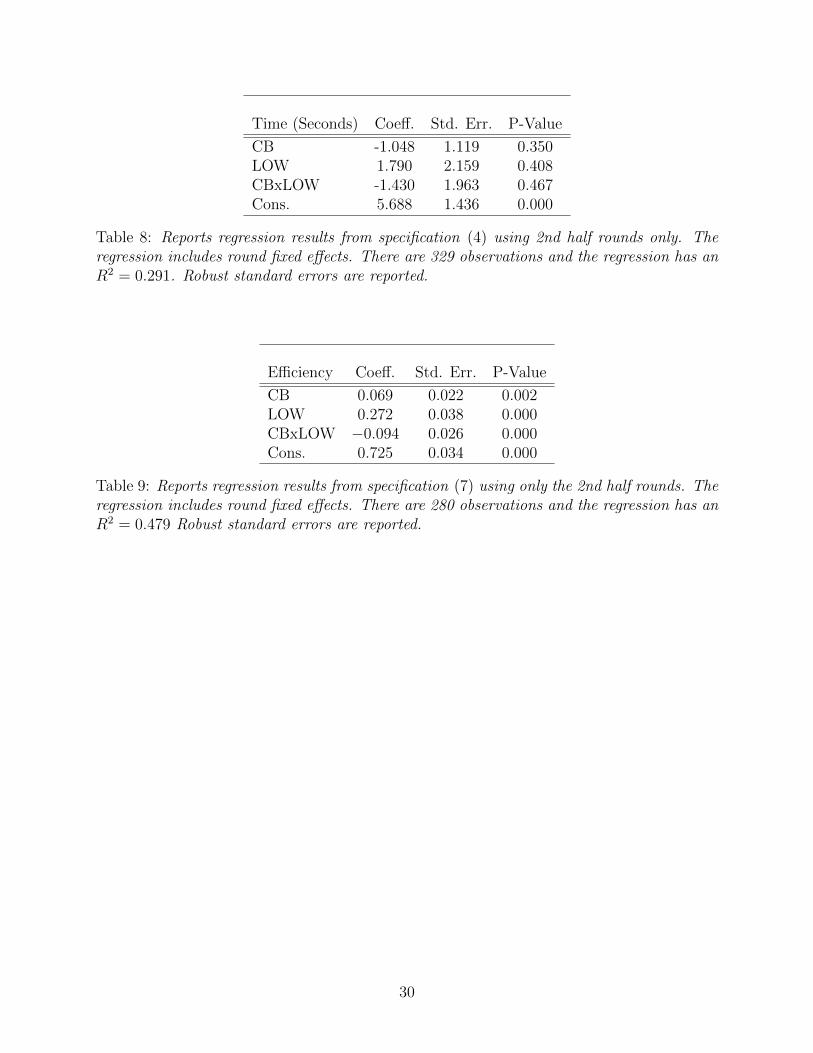
14Table 7 and Table 8 in the Appendix reports these results examining “bad” rounds only and roundsfrom the second half of the experiments, respectively.
20

the assets until the game ends) and the sum of payoffs realized by the investors given their
individual liquidation strategies.
Denoting K as the number of subjects who decide to sell their shares or are forced to do
so (if the state is bad), the total value realized in a market with N subjects is:
K∑k=1
pk−1 + (N −K)v (5)
The maximized total value, achieved if subjects follow the efficient liquidation rule and hold
on to their shares until the market game ends, is∑N
k=1 pk−1 in a bad state and Nv in a
good state. In bad state rounds welfare is always 100% because every unit is ultimately sold,
either voluntarily during the round or by force at the end of the round. As such, welfare can
only be suboptimal in “good” rounds, where it is given by:15
%Welfare ≡∑K
k=1 pk−1 + (N −K)v
Nv(6)
To examine the effect that a circuit breaker has on investor welfare we run the following
specification:16
%Welfareit = α0,t + α1CBit + α2LOWit + α3CBit ∗ LOWit + errorit (7)
Regression results are reported in Table 4.
15By construction, our measure of relative welfare simply rescales the number K of shares sold before theend of a round when the state is good. This measure is equal to 100% if K = 0, 85% if K = 1, 67.5% ifK = 2, 47.5% if K = 3 and 26.25% if K = 4.
16In this analysis, the first 5 rounds of data are excluded to allow subjects to have time to become familiarwith the trading environment. However, as is apparent in Figure 5, this learning may take long than 5rounds. As such, we also compare the efficiency between the CB and NoCB treatments only examining therounds in the second half of the sessions in Appendix B.
21
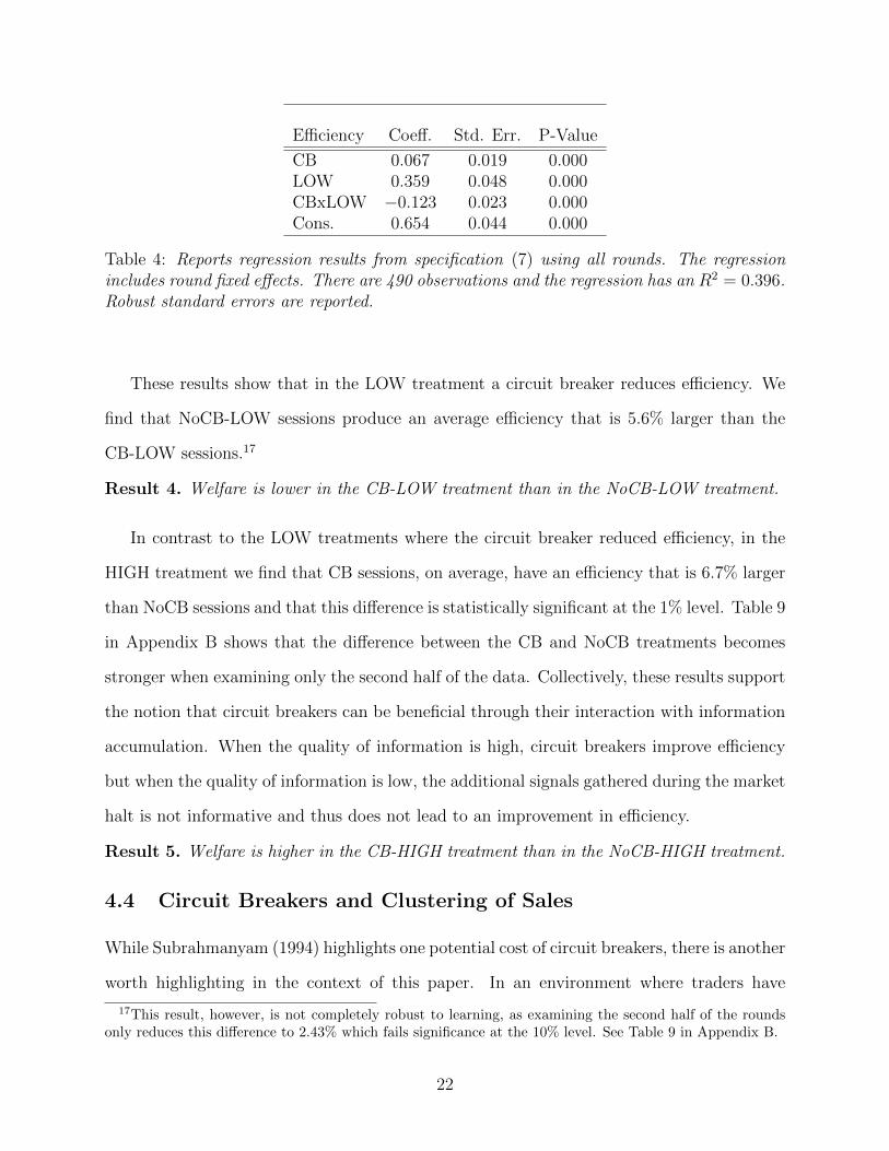
Efficiency Coeff. Std. Err. P-Value
CB 0.067 0.019 0.000LOW 0.359 0.048 0.000CBxLOW −0.123 0.023 0.000Cons. 0.654 0.044 0.000
Table 4: Reports regression results from specification (7) using all rounds. The regressionincludes round fixed effects. There are 490 observations and the regression has an R2 = 0.396.Robust standard errors are reported.
These results show that in the LOW treatment a circuit breaker reduces efficiency. We
find that NoCB-LOW sessions produce an average efficiency that is 5.6% larger than the
CB-LOW sessions.17
Result 4. Welfare is lower in the CB-LOW treatment than in the NoCB-LOW treatment.
In contrast to the LOW treatments where the circuit breaker reduced efficiency, in the
HIGH treatment we find that CB sessions, on average, have an efficiency that is 6.7% larger
than NoCB sessions and that this difference is statistically significant at the 1% level. Table 9
in Appendix B shows that the difference between the CB and NoCB treatments becomes
stronger when examining only the second half of the data. Collectively, these results support
the notion that circuit breakers can be beneficial through their interaction with information
accumulation. When the quality of information is high, circuit breakers improve efficiency
but when the quality of information is low, the additional signals gathered during the market
halt is not informative and thus does not lead to an improvement in efficiency.
Result 5. Welfare is higher in the CB-HIGH treatment than in the NoCB-HIGH treatment.
4.4 Circuit Breakers and Clustering of Sales
While Subrahmanyam (1994) highlights one potential cost of circuit breakers, there is another
worth highlighting in the context of this paper. In an environment where traders have
17This result, however, is not completely robust to learning, as examining the second half of the roundsonly reduces this difference to 2.43% which fails significance at the 10% level. See Table 9 in Appendix B.
22

imperfect information about the value of assets, strong negative information will lead to rapid
liquidations. While a circuit breaker may reduce the sale of valuable assets by giving agents
more time to gather information, it may also be the case that further negative information
accumulates during the market halt. In this case, the circuit breaker may result in a clustering
of trades when the market re-opens as traders now have stronger negative beliefs about the
asset than they did prior to the trading halt. We choose an example of this from the
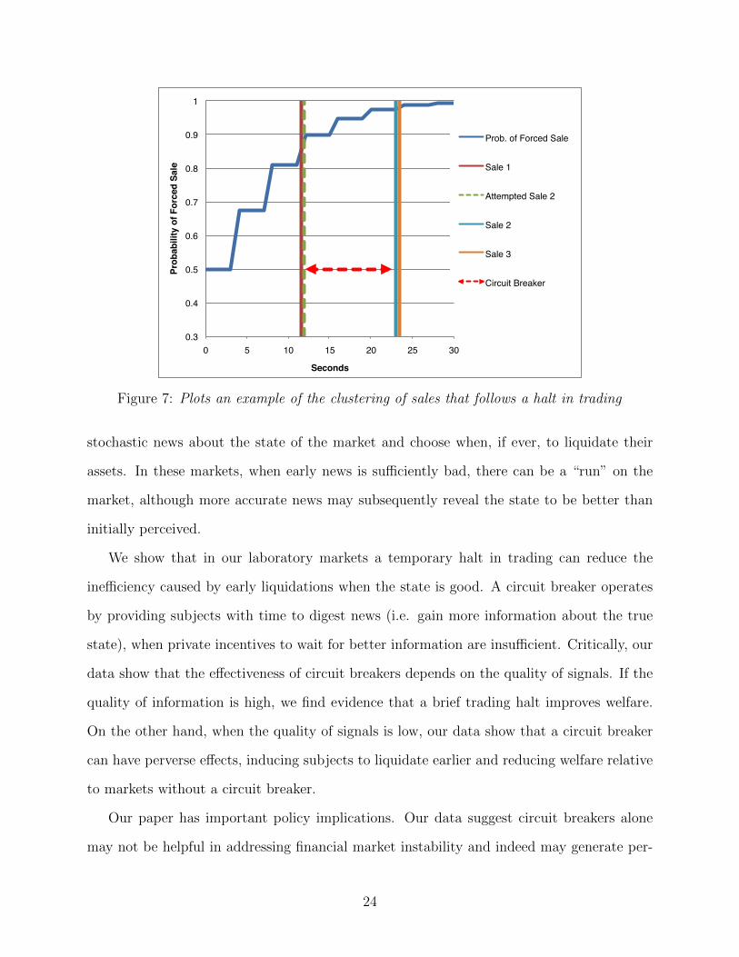
experiment and plot it in Figure 7. This figure depicts the evolution of the probability of
a forced liquidation (given by the blue line) in a bad state round. The vertical lines show
the time at which trades are entered to the market. After the third bad signal the first two
sale attempts occur in rapid succession. The first sale is executed and the second triggers
the circuit breaker, and is not executed. During the circuit breaker, more bad signals arrive
and the Bayesian updated probability of a forced liquidation stands at over 95% by the
end of the trading halt. When the market re-opens, two of the remaining traders rush to
liquidate their assets as there is now a very high probability that the round will end poorly.
In these sorts of cases a circuit breaker may induce a strong clustering of sales, when without
a circuit breaker it is likely those sales would have taken place over a more dispersed time
interval. The extent to which this clustering of sales may be undesirable is not necessarily
obvious, as in our experiment there is no efficiency cost associated with sales in “bad” rounds.
However, insofar as drastic price declines in short time intervals may have other undesirable
consequences, perhaps through their interaction with other behavioral phenomenon such as
herding or through their interaction with algorithmic trading, we view this potential side
effect of circuit breakers as worth highlighting, and to our knowledge has not been highlighted
in the literature to date.
5 Discussion
In this paper we explore the potentially efficiency-enhancing role of circuit breakers dur-
ing financial market runs. We implement a laboratory experiment where subjects receive
23
0.3!
0.4!
0.5!
0.6!
0.7!
0.8!
0.9!
1!
0! 5! 10! 15! 20! 25! 30!
Prob
abili
ty o
f For
ced
Sale!
Seconds!
Prob. of Forced Sale!
Sale 1!
Attempted Sale 2!
Sale 2!
Sale 3!
Circuit Breaker!
Figure 7: Plots an example of the clustering of sales that follows a halt in trading
stochastic news about the state of the market and choose when, if ever, to liquidate their
assets. In these markets, when early news is sufficiently bad, there can be a “run” on the
market, although more accurate news may subsequently reveal the state to be better than
initially perceived.
We show that in our laboratory markets a temporary halt in trading can reduce the
inefficiency caused by early liquidations when the state is good. A circuit breaker operates
by providing subjects with time to digest news (i.e. gain more information about the true
state), when private incentives to wait for better information are insufficient. Critically, our
data show that the effectiveness of circuit breakers depends on the quality of signals. If the
quality of information is high, we find evidence that a brief trading halt improves welfare.
On the other hand, when the quality of signals is low, our data show that a circuit breaker
can have perverse effects, inducing subjects to liquidate earlier and reducing welfare relative
to markets without a circuit breaker.
Our paper has important policy implications. Our data suggest circuit breakers alone
may not be helpful in addressing financial market instability and indeed may generate per-
24

verse effects in poor information environments. On the other hand, combining mandated
trading halts with policies aimed at improving information disclosure may prevent full mar-
ket runs from occurring unnecessarily in illiquid markets. In addition, future research on the
specific rules and features of circuit breakers would also be a productive agenda. Specifically,
understanding the optimal trigger rules and length of a market halt could help design op-
timal circuit breaker policies. Our findings suggest that the length of a market halt should
be given special attention. On one hand, longer market halts would provide more informa-
tion accumulation and prevent market runs when the state is “good,” but could also lead
to extreme volatility, as highlighted in Figure 7, when the state is “bad.” Finally, while in
this paper we assume information is exogenous, one important way in which this framework
can be extended is by letting investors decide how and when to obtain new signals. Study-
ing the interaction between circuit breakers and the investors’ incentives to acquire better
information is an important avenue for future research.
References
Ackert, L., Church, B. and Jayaraman, N. (2001). An experimental study of circuit breakers:
The effects of mandated market closures and temporary halts on market behavior,
Journal of Financial Markets 4(2): 185–208.
Ackert, L., Church, B. and Jayaraman, N. (2005). Circuit breakers with uncertainty about
the presence of informed agents: I know what you know i think, Financial Markets,
Institutions & Instruments 14(3): 135–168.
Allen, F. and Gale, D. (2000). Financial contagion, Journal of political economy 108(1): 1–33.
Angstadt, J. (2011). What will be the legacy of the flash crash? developments in US equities
market regulation, Capital Markets Law Journal 6(1): 80–91.
Arifovic, J., Jiang, J. and Xu, Y. (2011). Experimental evidence of bank runs as pure
coordination failures, Technical report.
25

Bernanke, B. and Gertler, M. (1990). Financial fragility and economic performance, The
Quarterly Journal of Economics pp. 87–114.
Bernardo, A. and Welch, I. (2004). Liquidity and financial market runs, The Quarterly
Journal of Economics 119(1): 135–158.
Brady Commission (1988). Report of the presidential task force on market mechanisms, US
Government Printing Office.
Brunnermeier, M. K. and Morgan, J. (2010). Clock games: Theory and experiments, Games
and Economic Behavior 68(2): 532–550.
Chakrabarty, B., Corwin, S. A. and Panayides, M. A. (2011). When a halt is not a halt: An
analysis of off-nyse trading during nyse market closures, Journal of Financial Interme-
diation 20(3): 361–386.
Cheung, Y.-W. and Friedman, D. (2009). Speculative attacks: A laboratory study in con-
tinuous time, Journal of International Money and Finance 28(6): 1064–1082.
Corwin, S. A. and Lipson, M. L. (2000). Order flow and liquidity around nyse trading halts,
The Journal of Finance 55(4): 1771–1801.
Diamond, D. and Dybvig, P. (1983). Bank runs, deposit insurance, and liquidity, The journal
of political economy pp. 401–419.
Draus, S. and Van Achter, M. (2016). Circuit breakers and market runs. Working Paper.
Engelen, P.-J. and Kabir, R. (2006). Empirical evidence on the role of trading suspensions
in disseminating new information to the capital market, Journal of Business Finance
& Accounting 33(7-8): 1142–1167.
Greenwald, B. and Stein, J. (1991). Transactional risk, market crashes, and the role of circuit
breakers, Journal of Business pp. 443–462.
26

Greiner, B. (2015). Subject pool recruitment procedures: organizing experiments with orsee,
Journal of the Economic Science Association 1(1): 114–125.
Hauser, S., Kedar-Levy, H., Pilo, B. and Shurki, I. (2006). The effect of trading halts on the
speed of price discovery, Journal of Financial Services Research 29(1): 83–99.
Kendall, C. (2015). Rational and heuristic-driven trading panics in an experimental asset
market. Working Paper.
Kim, Y. and Yang, J. (2004). What makes circuit breakers attractive to financial markets?
a survey, Financial Markets, Institutions & Instruments 13(3): 109–146.
Kodres, L. and O’Brien, D. (1994). The existence of pareto-superior price limits, The Amer-
ican economic review pp. 919–932.
Madies, P. (2006). An experimental exploration of self-fulfilling banking panics: Their oc-
currence, persistence, and prevention, The Journal of Business 79(4): 1831–1866.
Madura, J., Richie, N. and Tucker, A. L. (2006). Trading halts and price discovery, Journal
of Financial Services Research 30(3): 311–328.
Pettit, J., Hewitt, J. and Oprea, R. (2014). Redwood: Software for graphical, browser based
experiments in discrete and continuous time, Technical report.
Schotter, A. and Yorulmazer, T. (2009). On the dynamics and severity of bank runs: An
experimental study, Journal of Financial Intermediation 18(2): 217–241.
Subrahmanyam, A. (1994). Circuit breakers and market volatility: A theoretical perspective,
Journal of Finance 49(1): 237–54.
27
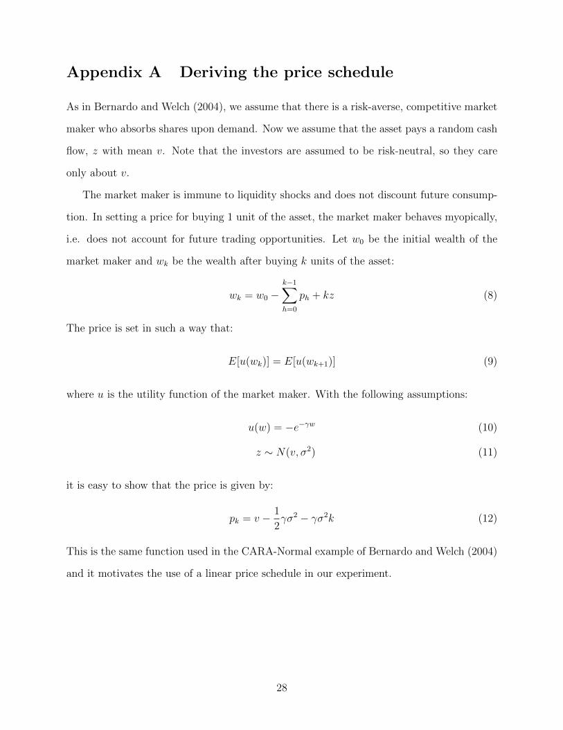
Appendix A Deriving the price schedule
As in Bernardo and Welch (2004), we assume that there is a risk-averse, competitive market
maker who absorbs shares upon demand. Now we assume that the asset pays a random cash
flow, z with mean v. Note that the investors are assumed to be risk-neutral, so they care
only about v.
The market maker is immune to liquidity shocks and does not discount future consump-
tion. In setting a price for buying 1 unit of the asset, the market maker behaves myopically,
i.e. does not account for future trading opportunities. Let w0 be the initial wealth of the
market maker and wk be the wealth after buying k units of the asset:
wk = w0 −k−1∑h=0
ph + kz (8)
The price is set in such a way that:
E[u(wk)] = E[u(wk+1)] (9)
where u is the utility function of the market maker. With the following assumptions:
u(w) = −e−γw (10)
z ∼ N(v, σ2) (11)
it is easy to show that the price is given by:
pk = v − 1
2γσ2 − γσ2k (12)
This is the same function used in the CARA-Normal example of Bernardo and Welch (2004)
and it motivates the use of a linear price schedule in our experiment.
28
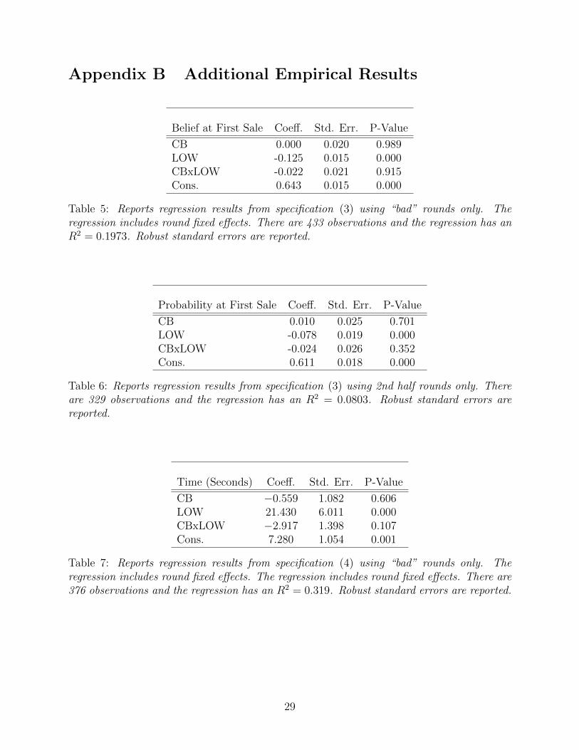
Appendix B Additional Empirical Results
Belief at First Sale Coeff. Std. Err. P-Value
CB 0.000 0.020 0.989LOW -0.125 0.015 0.000CBxLOW -0.022 0.021 0.915Cons. 0.643 0.015 0.000
Table 5: Reports regression results from specification (3) using “bad” rounds only. Theregression includes round fixed effects. There are 433 observations and the regression has anR2 = 0.1973. Robust standard errors are reported.
Probability at First Sale Coeff. Std. Err. P-Value
CB 0.010 0.025 0.701LOW -0.078 0.019 0.000CBxLOW -0.024 0.026 0.352Cons. 0.611 0.018 0.000
Table 6: Reports regression results from specification (3) using 2nd half rounds only. Thereare 329 observations and the regression has an R2 = 0.0803. Robust standard errors arereported.
Time (Seconds) Coeff. Std. Err. P-Value
CB −0.559 1.082 0.606LOW 21.430 6.011 0.000CBxLOW −2.917 1.398 0.107Cons. 7.280 1.054 0.001
Table 7: Reports regression results from specification (4) using “bad” rounds only. Theregression includes round fixed effects. The regression includes round fixed effects. There are376 observations and the regression has an R2 = 0.319. Robust standard errors are reported.
29
Time (Seconds) Coeff. Std. Err. P-Value
CB -1.048 1.119 0.350LOW 1.790 2.159 0.408CBxLOW -1.430 1.963 0.467Cons. 5.688 1.436 0.000
Table 8: Reports regression results from specification (4) using 2nd half rounds only. Theregression includes round fixed effects. There are 329 observations and the regression has anR2 = 0.291. Robust standard errors are reported.
Efficiency Coeff. Std. Err. P-Value
CB 0.069 0.022 0.002LOW 0.272 0.038 0.000CBxLOW −0.094 0.026 0.000Cons. 0.725 0.034 0.000
Table 9: Reports regression results from specification (7) using only the 2nd half rounds. Theregression includes round fixed effects. There are 280 observations and the regression has anR2 = 0.479 Robust standard errors are reported.
30

Appendix C Experiment Instructions
This section reproduces instructions given to experiment subjects for the baseline CB ses-
sions.
Instructions
You are about to participate in an experiment in the economics of decision-making. The
National Science Foundation and other agencies have provided the funding for this project.
If you follow these instructions carefully and make good decisions, you can earn a CONSID-
ERABLE AMOUNT OF MONEY, which will be PAID TO YOU IN CASH at the end of
the experiment.
Your computer screen will display useful information. Remember that the information
on your computer screen is PRIVATE. To insure best results for yourself and accurate data
for the experimenters, please DO NOT COMMUNICATE with the other participants at any
point during the experiment. If you have any questions, or need assistance of any kind, raise
your hand and one of the experimenters will come.
Rounds
The experiment will be divided into 55 rounds. The length of a round will be random
– you will never know how long a round will last or when it is about to end (details below).
When a round ends, your experiment will show a round summary page in red for a few
seconds and then a new round will begin. Decisions and points made in one round do not
affect other rounds.
The Basic Idea
You and three other players are traders market where an asset is traded. Each round you
start the game with one unit of a asset. Your only decision is when, if ever, to sell
your asset. First, we will describe what happens if you decide to sell the asset before the
31

end of the round and then we will describe what happens if you decide to keep the asset
until the end of the round.
32

Selling
At any moment you can decide to sell the asset. If you sell the asset, the asset is bought
by the computer and you are paid a price. The amount you will be paid depends only
on how many other participants have already sold their asset: each sale of a asset lowers
its price. The exact price schedule the computer will use is reproduced in Table 10. For
example: if you decide to sell and you are the first to sell you will be paid a price of $8 ; if 1
unit has already been sold (by the another participant) and you decide to sell now, you will
be paid a price of $6, etc.
Price scheduleNumber of assets already sold Price you are paid if you sell
0 81 62 43 2
Table 10: Price Schedule
Holding on to the asset
What if you have decided not to sell your asset and the round randomly ends? One of the
following will occur:
1. Forced Sale: You are forced to sell your asset, together with all the other players who
are still in possession of their assets. Your points in this round are given by the price
at which your asset is sold (see more below). or
2. Payout: You and all the other player(s) who decided not to sell receive the asset
payout, equal to 20 points.
The computer will randomly decide whether the round ends in a Forced Sale or Fixed
Payout. Each round has a 50% probability of ending with a Forced Sale and 50% probability
of ending with the Fixed Payout.
33

Figure 1 illustrates what can happen at the end of a round and how this affects your
score if you have not sold your asset by then.
End ofround
PAYOUTpoints=20
FORCED SALEpoints=price
(see Table 1)
50% of cases
50% of cases
Figure 8: Points if you have not sold before the random end
Forced sales
When the round ends in a forced sale the computer will randomly decide the selling order
for those players who have not sold earlier and pay each player in that order according to
the schedule in Table 10. Examples:
• If none of the participants have decided to sell in the round and the round ends in a
forced sale, the computer will randomly decide the selling order of the four participants.
The first player will receive 8 points, the second 6 points, the third 4 points and the
fourth 2 point.
• If two players decided to sell earlier in the round and the round ends in a forced sale
the computer will randomly order the remaining 2 participants. The first participant
will receive 4 points and the second 2 point.
The likelihood that the asset pays out
Whether a forced sale will occur in a particular round will not be known to you until it
happens. However, you will receive real-time signals about whether a Forced Sale
34

will occur.
During the round you will receive either a Good or Bad signal every 4 seconds. On
your computer screen you will be shown whether the current message is Good or Bad and
a tally of the Good and Bad signals received so far in that round. For example, if a good
signal arrives you may see +Good (+2/-3). This message indicates that the current signal
is Good and that there have been 2 Good signals and 3 Bad signals so far in the round.
This tally of signals will be updated every 4 seconds, until the round ends. In each round
the signal tally will begin at (+0/-0). Over time the Bad tally will become larger than the
Good tally if a Forced Sale will occur. Conversely, over time the Good tally will become
larger than the Bad tally if a Payout will occur.
Here are some details on the probability that a Good signal or a Bad signal arrives at
each update. If in this round a Forced Sale will occur, then the probability that a Bad
signal arrives is 67.5% and the probability that a Good signal arrives is 32.5%. If in this
round the assets will Payout, then the probability that a Bad signal arrives is 32.5% and the
probability that a Good signal arrives is 67.5%. Therefore at each update, a Bad signal is
more likely to arrive if a Forced Sale will occur at the end of the round and a Good signal
is more likely to arrive if a Payout will occur at the end of the round.
Market Freeze
During each round the market may freeze. During a market freeze your sell button will be
disabled and you will be unable to sell your asset. The market will freeze when too many
players attempt to sell their assets at once. Specifically, if one player sells their asset and
another player attempts to sell their asset within 3 seconds of that sale the market will freeze.
In this case the first sale will go through but the second will not. The market will unfreeze
after 10 seconds at which point any participant who still owns an asset is again able to sell
it if they choose to. The market can only freeze once per round. You will be notified when
35

the market is frozen in the Market Status part of your screen.
36

Screen Information
The screenshot reproduced in Figure 9 shows an example of the screen you will see during
each round.
The table at the top of the screen shows you the current signal and the tally of Good
and Bad signals. You will see the signals and tallies updating during the experiment.
The plot shows you the current price that you can obtain if you sell your asset now,
as a yellow line (remember this is entirely determined by how many people have already
sold). The rightmost tip (the leading edge) of the line shows what is happening right now.
Whenever some player sells his or her asset you will see a discrete jump in this line.
At any moment you can sell your asset by clicking the button at the bottom of the screen
that says Sell. However remember that your sale goes through, the button will be disabled
for the rest of the round.
Figure 9: Example Screen View
37

Feedback
After the round is over, you will be shown a summary message in your page repeating your
score and whether a forced sale occurred. The break between rounds will last around 10
seconds. During this break you will see: 1) your score in this round, 2) whether you sold
your asset by clicking on the button during the round, 3) how the round ended: Forced Sale
or Payout.
Earnings
At the end of the last round, you will be paid $7.00, plus earnings based on your
total points throughout the experiment.
At the end of the experiment you will be presented with a summary table with your
earnings in each round and your total earnings in the experiment. The points you earn in
the experiment will be converted to U.S. Dollars at an exchange rate of 55 to 1. THAT IS,
FOR EACH 55 POINTS YOU EARN IN THE EXPERIMENT YOU WILL BE
PAID 1 Dollar.
38

Details
Here are a few more details on the experiment, in case you want to know.
How long will a round last?
• The minimum round length is eight seconds.
• The actual round length is random. The round ends with some constant probability
every four seconds.
• The average length of a round is 32 second. Many rounds will last less than the average,
and a few will last much longer.
• Rounds longer than a couple of minutes are so unlikely that you probably will never
see one.
Frequently Asked Questions
Q1. Is this some kind of psychology experiment with an agenda you haven’t told us?
Answer: No. It is an economics experiment. If we do anything deceptive, or don’t pay you
cash as described, then you can complain to the campus Human Subjects Committee
and we will be in serious trouble. These instructions are meant to clarify how you earn
money, and our interest is in seeing how people make market decisions.
39

40