Written for a special edition of ZDM entitled Transforming Mathematics Education through the use of Dynamic Mathematics due for publication June 2009

Dynamic mathematics and the blending of knowledge structures in the calculus

David Tall, University of Warwick

This paper considers the role of dynamic aspects of mathematics specifically focusing on the calculus, including both physical human action and computer software that responds to physical action to produce dynamic visual effects. The development builds from dynamic human embodiment, uses arithmetic calculations in computer software to calculate ‘good enough’ values of required quantities and algebraic manipulation to develop precise symbolic values. The approach is based on a developmental framework blending human embodiment, with the symbolism of arithmetic and algebra leading to the formalism of real numbers and limits. It builds from dynamic actions on embodied objects to see the effect of those actions as a new embodiment that needs to be calculated accurately and symbolised precisely. The framework relates the growth of meaning in history to the mental conceptions of today’s students, focusing on the relationship between potentially infinite processes and their consequent embodiment as mental concepts. It broadens the strategy of process-object encapsulation by blending embodiment and symbolism.

1. Introduction The calculus of Newton and Leibniz is the crowning glory of classical mathematics. Our modern approach is based on the limit concept, which is known to cause serious problems for students. In this paper I will present a framework for developing mathematical thinking from embodiment to symbolism and on to formal mathematical concepts that reveals how how the students mental conceptions of limits relate to the historical conceptions of potentially infinite processes that lead naturally to infinitesimal conceptions. The dynamic nature of computer graphics allows limiting processes to be seen as stabilising on a recognisable embodied object that can be calculated arithmetically and formulated symbolically, giving a link between embodiment,

symbolism and fundamental concepts of the calculus. Calculus begins with the desire to quantify how things change (the function concept), the rate at which they change (the derivative), the way in which they accumulate (the integral), and the relationship between the two (the fundamental theorem of calculus and the solution of differential equations). Calculus is fundamentally a dynamic conception. Even the calculation of static quantities—such as areas or volumes—involve dynamic processes of adding up a large number of very tiny elements to build up the given shapes. The nineteenth century transformation of dynamic calculus into quantified epsilon-delta definitions developed the formal theory of mathematical analysis used by the professional mathematicians of today. This has led to the teaching of calculus based on the limit concept, which satisfies the logical needs of mathematicians but proves to be complicated for students. In the approach suggested here, the student builds on knowledge structures that are likely to be more familiar: dynamic human embodiment to give enlightened meaning to calculus concepts, ‘good enough’ arithmetic to calculate to a desired accuracy, and symbolic formulation to give precise conceptions.

2. A framework for the development of mathematical thinking In the framework of mathematical thinking given here I will show how the underlying mental processes that allowed our predecessors to invent the calculus are directly related to the conceptions that occur in our students. They relate to how we as human beings perceive the changing world.

2.1 Human embodiment

Our brains make sense of the world by assembling neuronal information from our senses and our existing memories to form a ‘selective binding’ of different aspects of thought into a single phenomenon. Merlin Donald, in his exquisite book, A Mind So Rare (2001), sees this as the first of three distinct levels of consciousness. Selective binding occurs automatically in milliseconds, around a fortieth of a second or so. It builds a gestalt that takes account of many aspects of the situation. The second level of consciousness he terms ‘short-term awareness’, which links

2

together events over a period of seconds to give us a conscious flow of thought. The third level, ‘extended awareness’, links together events over periods of minutes or hours. The combination of selective binding and short-term awareness give us a continuous dynamic view of the world, enabling us to see a video at 25 to 30 still frames a second as a continuous sequence of events that can be displayed on a computer screen as a dynamic moving picture. Short-term awareness enables us to sense the world in dynamic terms. Our extended awareness enables us to reflect on our perceptions and actions to interpret them in imaginative ways. Even though our perception is limited by the biological workings of our brain, our thought processes enable us to build on what we see to imagine new possibilities beyond the limitations of the human frame. We can imagine points with position and no size, lines with length and no breadth, perfect circles and platonic solids. We can amplify our thoughts using tools, such as magnifying glasses to look closely at things, or extremely fast cameras to take many more pictures a second and slow the result down to see actions in shorter periods of time in slow motion. We can design dynamic software that enables the individual to interact with calculus concepts to gain insights that are not evident in static pictures. In the next section I will present a framework for the development of mathematical thinking that builds on the natural resources available to Homo sapiens as a species and hypothesise how these resources are used to build sophisticated mathematical ideas, with particular reference to the dynamical ideas in the calculus. The same framework has implications for the historical development of mathematics within different societies and the development of the individual within today’s society. I will then use the framework to consider the historical conceptions in the calculus, the conceptual development of students in today’s society and the use of the computer to give new dynamic insights into calculus concepts. The phenomenon of a graphic approach to calculus using computer graphics has been with us for over a quarter of a century (Tall, 1981). This paper underpins the ongoing data with a new theoretical framework blending embodiment and symbolism.

2.2 Three mental worlds of mathematics

In recent years I have been building a framework of cognitive development in mathematical thinking that grows from the perceptions and actions of the child to the formal productions of the mathematician. This is postulated to occur through three mental worlds of mathematics (Tall, 2004, 2008):

the (conceptual) embodied world, based on perception of and reflection on properties of objects, initially seen and sensed in the real world but then imagined in the mind; the (procedural-proceptual) symbolic world that grows out of the embodied world through action (such as counting) and is symbolised as thinkable concepts (such as number) that function both as processes to do and concepts to think about (procepts); the (axiomatic) formal world (based on formal definitions and proof), which reverses the sequence of construction of meaning from definitions based on known objects to formal concepts based on set-theoretic definitions.

The terms ‘embodiment’, ‘symbolism’ and ‘formalism’ are used with a variety of meanings in linguistics, philosophy and psychology. Here, they will be used in conjunction with the meaning given by their qualifying adjectives: ‘conceptual embodiment’, ‘procedural-proceptual symbolism’ ‘axiomatic formalism’. These meanings capture the different ways in which we humans make sense of mathematics within the conceptual framework of three developing mental worlds of mathematics. It transpires that these three worlds build naturally from three fundamental human abilities, which I term ‘set-befores’ as they are set before our birth in our genes and develop naturally through our social experiences in life: recognition of similarities, differences and

patterns, repetition of actions to make them routine, language to name phenomena to talk about them and refine their meaning.

These three set-befores lead to three distinct ways of constructing concepts formulated by Gray and Tall (2001),

Recognition supported by language enables categorisation, Repetition makes procedural learning possible and, suitably supported by language, it also

3

allows actions to be symbolised and considered as procepts through encapsulation, Language enables definition, initially through description of phenomena, and then in terms of formal set-theoretic definition.

I hypothesize that this framework underlies the growth of mathematical thinking both in terms of the ways that individuals grow from childhood to maturity, and also in the way that ideas develop historically. The child begins with embodiment, developing proceptual symbolism in arithmetic, algebra and calculus, and some go on to become mathematicians, formalising theories in set-theoretic terms. The adults who feature in history have already matured through such a development and, as adults, their conceptions of embodiment and symbolism underlie the growth of mathematical thinking in history, accompanied by the linguistic development of euclidean proof building coherent deductive theories based on embodiment and the later set-theoretic formalism of the late nineteenth and early twentieth century giving us our modern axiomatic framework.

2.3 Historical development of the calculus

The development of calculus over the centuries can be fruitfully modelled in the three-world framework. The Greek idea of the potential infinity of subdividing a quantity again and again builds on the set-before of repetition allowing a potential infinity of repetitions. The categorisation of potential infinity depends on the manner in which the repetitions operate. In the case of the sequence of counting numbers, the set-before of recognition allows the categorisation of the repeating sequence of natural numbers as an actually infinite set which is readily accepted by our students (Tall, 1980a). However, the repetition of a process with an underlying pattern of successive states is likely to focus attention on this pattern, leading to a natural human belief that the limiting object is endowed with the same properties as the individual terms. I termed this phenomenon a generic limit concept (Tall, 1986, 1991a). For instance, if a quantity repeatedly gets smaller and smaller and smaller without ever being zero, then the limiting object is naturally conceptualised as an extremely small quantity that is not zero (Cornu, 1991). Infinitesimal concepts are natural products of the human imagination derived through combining potentially infinite repetition and the recognition of its repeating properties.

The physical and mental possibilities of such subdivisions are different. Try cutting a strip of paper in half, then cut one of these halves into a half again, and so on to see how many bisections can be made. Not many. Indeed, when I wrote the book Foundations of Mathematics with Ian Stewart (1976), I enquired of my friends in physics how big was the estimated size of the known universe and how many times it could be cut in half before the cut was less than the size of an electron, and, to my amazement, the answer was 81! Physically we cannot go on dividing a quantity in half for very long, but, theoretically our arithmetic symbolism tells us that we have potentially infinite sequence, 1, 12 , 14 , … where the terms can successively be halved ad infinitum. The Greeks presented the dichotomy of potential and actual infinity by questioning whether subdivision can go on potentially for ever, or whether it reaches a point where tiny indivisibles cannot be further divided. They also found subtle problems in dealing with these ideas. Democritus calculated the volume of a cone by slicing it into thin sections parallel to the base and added up the volumes of these sections. However, he had the problem of deciding whether the successive sections were equal or unequal, for if unequal, then the curved surface of the cone would have a sequence of steps, but if equal, then the cone would be a cylinder. (Heath, 1921). In the revival of mathematics in renaissance times, Nicholas of Cusa (1401-1464) considered the circle as a regular polygon with an infinite number of sides, which Kepler (1571-1630) took further by formulating a metaphysical ‘bridge of continuity’ between a regular polygon with a large number of sides and a circle, or between an infinitesimal area and a line, or between the finite and the infinite. He considered a sphere made up of an infinite number of infinitesimally thin cones with vertex at the centre and bases making up the surface; this enabled him to use the volume of a cone as one-third base times height to add them all together to give the total volume of the sphere as one third the surface area times the radius. Leibniz formulated a similar ‘principle of continuity’, claiming in that:

In any supposed transition, ending in any terminus, it is permissible to institute a general reasoning, in which the final terminus may also be included.

4

It was the inability of Homo Sapiens to resolve conflicts related to the concepts of infinity and infinitesimal that led to the formal construction of numbers by Dedekind cuts or Cauchy sequences and introducing a quantified version of the concept of limit. This new definition formulated the convergence of a sequence

(a

n) to a limit a in

the form of a challenge: given a desired accuracy within an error of at most ! > 0 , find a whole number N so that the terms

a

n for n > N are all

within an error ! of a. In this new formulation, the symbols refer to specific terms in quantified statements, however, we still use metaphors to speak of the terms of a sequence ‘varying’ and

a

n

‘getting close’ to a as N ‘increases’. The insight of Robinson (1966) to formulate a new logical theory of infinitesimals was seen by him as a solution to the long dispute over the status of infinitesimals, but mathematicians with brains steeped in the experiences of mathematical analysis chose to maintain their allegiance to the status quo. As a consequence the calculus is still taught to students in terms of the limit concept, with quantities getting ‘as close as desired’ which in practice leads to the notion of a generic limit. For instance, the infinite decimal 0.999… is intended to signal the limit of the sequence 0.9, 0.99, 0.999, … which is 1, but in practice it is often imagined as a limiting process which never quite reaches 1.

2.4 A formal view of infinitesimals

Robinson’s idea of infinitesimals was used for a time to teach undergraduates the calculus in the USA (Keisler, 1976) while the market continues to be dominated by the widespread use of compendious text books such as Stewart (2003) which retain traditional approaches to calculus familiar to instructors, with the addition of dynamic software. However, one advance made by Robinson that is of real value is the formal notion of an infinitesimal, which gives a formal underpinning to the embodied idea of ‘magnifying’ graphs to see differentiable functions look ‘locally straight’. In Tall (2002) I gave examples of ordered fields that are extensions of the real numbers ! and showed how they could be visualised as a number line. If K is such an extension field, any element in K is either greater than every element in ! , in which case it is defined to be positive infinite, or less than every element in ! (negative infinite) or between two elements of ! , in which case it is

said to be finite. A non-zero element in K that lies between !r and r for any positive r !! is said to be an infinitesimal. It is elementary to use the completeness of ! to show that any finite element of x !K is uniquely of the form c + ! where c is real (called the standard part of x, denoted by st(x)) and ! is either infinitesimal or zero. The derivative of a function

y = f (x) , if it exists, is defined to be

!f (x) = stf (x + h)" f (x)

h

#

$%&

'(

for infinitesimal h. For instance, for f (x) = x2 the

derivative is

st(x + h)2 ! x

2

h

"

#$%

&'= st(2x + h) = 2x .

We can magnify the plane K ! K by taking fixed a, b, c, d !K , and defining

µ(x, y) =x ! a

c,

y ! b

d

"

#$%

&'

This is called a (c,d) -lens pointed at

(a,b) . We

call the set of points (x, y) where

(x ! a) / c and

( y ! b) / d are both finite the field of view of the lens µ . I speak of an optical lens o taking

(x, y) in the field of view to

o(x, y) = stx ! a

c

"

#$%

&',st

y ! b

d

"

#$%

&'"

#$%

&'.

The image o(x, y) is then a point in the real

plane. Pointing an optical lens at

(a, f (a)) on a graph using an infinitesimal c = d = ! , then any point

(a + h, f (a + h)) on the graph in the field of view is transformed to

sta + h ! a

"#

$%&

'(, st

f (a + h)! f (a)

"#

$%&

'(#

$%&

'(

= sth

!"

#$%

&', st

h

!"

#$%

&'st

f (a + h)( f (a)

h

"

#$%

&'"

#$%

&'.

The original point (a + h, f (a + h)) is therefore in

the field of view if and only if h / ! is finite, and its image is then

!,! "f (x)( )

where ! = st(h / " ) is a real number. As ! is an

infinitesimal, h must also be an infinitesimal (otherwise h / ! would be infinite). For a differentiable function f, the visible points

(!,! "f (x)) form a straight line in !2 with

slope !f (x) and real parameter ! . The infinite

optical magnification of a differentiable function f

5

at a point (x, f (x)) is therefore an infinite straight

real line of slope !f (x) .

It is this knowledge that gave me the personal confidence to declare a locally straight approach to calculus (Tall, 1985). My intention has never been to teach students a new theory of infinitesimals when they first meet the calculus, but to build a new approach based on dynamic human embodiment. The first step in this approach is to zoom in on a graph dynamically to see it close under high magnification.

2.5 The Leibniz notation and local straightness

The Leibniz notation remains the fundamental symbolism used in the calculus because it is so very useful. However, over the centuries its meaning has changed as Bolzano insisted that the symbol

dy / dx should not be seen as a ratio of dy to dx but as the limit of

( f (x + !x)" f (x)) / !x as !x tends to zero. Subsequently this led to a dysfunctional approach to the calculus which still prevails today in which

dy / dx is a limit, not a quotient, the dx in the integral

! f (x) dx is not the same as the dx in

dy / dx , but means ‘the integral of

f (x) with respect to x’, yet the differential equation

dy

dx= !

x

y

is solved by ‘cross-multiplying’ to get y dy = !x dx which is integrated to get

y dy! = " x dx!

with solution

x

2+ y

2= c .

This confusing mixture of ideas does no favours for meaningful understanding of the calculus. Yet Leibniz’s first definition of dx and dy was to let dx be any non-zero number and dy to be the value such that the ratio of dy to dx is the same as the ratio of y to the subtangent BX (figure 1).

Figure 1: The Leibniz definition of dx, dy

This picture with dx and dy as the components of the tangent vector is found in modern textbooks. Its static nature fails to convey the vision in Leibniz’s mind. However, if we take a graph such as

y = x

2 with very small values of dx and dy, then on high magnification (as suggested by Robinson’s insight), the magnified graph will look like a straight line so that the graph and its tangent are now indistinguishable (figure 2).

figure 2: A graph under high magnification

This picture now seems to show the value of dy going up to the graph itself. There is still an error, but it is contained within the thickness of the line in the drawing. This is related to the idea of Leibniz that the addition of a line to an area does not affect its area as what is added is of a smaller order of size. By choosing a suitably small value of dx, we can see

dy / dx , as the slope of the tangent, now a ‘good enough’ approximation to give a visual representation for the slope of the graph itself.

3. A locally straight approach to calculus The purpose of a locally straight approach to the calculus is to use students’ knowledge built up before meeting the calculus to smooth the passage to the imaginative ideas of changing slope and growing areas. It builds on the student’s embodied imagination of graphs that can be magnified dynamically on a visual display to look locally straight. It also has the advantage that it gives an embodied meaning to the Leibniz notation as the ratio of the components of the tangent vector. When the graph of a function is plotted on the screen what we see is not the ‘perfect’ graph of a line with no thickness, but a string of pixels of finite size that covers the theoretical graph and draws a practical version. This can be embodied by tracing a finger along the graph, which not only traces along a visual object, it also embodies

6

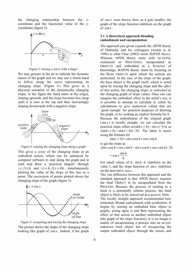
the changing relationship between the x-coordinate and the functional value of the y-coordinate (figure 3).

Figure 3: tracing a curve with a finger

We may gesture in the air to indicate the dynamic nature of the graph and we may use a whole hand to follow along the curve representing its changing slope. (Figure 4.) This gives us a physical sensation of the dynamically changing slope; in the figure the hand starts at the origin, sloping upwards, and the slope becomes less steep until it is zero at the top and then increasingly sloping downwards with a negative slope.

Figure 4: sensing the changing slope along a graph

This gives a sense of the changing slope as an embodied action, which can be enhanced by computer software to step along the graph and at each step draw a ‘practical tangent’ through

(x, f (x)) and (x + h, f (x + h)) , simultaneously

plotting the value of the slope of this line as a point. The succession of points plotted shows the changing slope of the graph (figure 5).

Figure 5: computing and tracing the changing slope

The picture shows the shape of the changing slope looking like graph of cos x . Indeed, if the graph

of cos x were drawn, then, as h gets smaller, the graph of the slope function stabilises on the graph of cos x .

3.1 A theoretical approach blending embodiment and encapsulation

The approach just given expands the APOS theory of Dubinsky and his colleagues (Asiala et al, 1996) to what Chae (2002) terms BAPOS theory. Whereas APOS theory starts with ACTIONS, routinized as PROCESSES, encapsulated as OBJECTS and embedded in a SCHEMA of knowledge, BAPOS theory starts by focusing on the BASE OBJECTS upon which the actions are performed. In the case of the slope of the graph, the base object is the graph itself, which is acted upon by tracing the changing slope and the effect of this action, the changing slope, is embodied as the changing graph of slope values. Once one can imagine the embodied effect in the mind’s eye, it is possible to attempt to calculate it, either by calculations to give numerical values that are ‘good enough’ for practical purposes of drawing the graph, or by seeking an explicit formula for it. Because the embodiment of the original graph ( sin x ) is locally straight, we can calculate the practical slope either as

(sin(x + h)! sin x) / h or as

(sin(x + h)! sin(x ! h)) / 2h . The latter is easier using the formula for

sin(x + h) = sin x cos h + cos x sin h

to get the slope as (sin x cos h + cos x sin h ! sin x cos h + cos x sin h) / 2h

= cos xsin h

h.

For small values of h, sin h / h stabilises on the

value 1, and the slope function of sin x stabilises on the derivative cos x . The vast difference between this approach and the standard approach is that APOS theory requires the final OBJECT to be encapsulated from the PROCESS. Because the process of tending to a limit is a potentially infinite process, the limit object is likely to be conceived as a generic limit. The locally straight approach recommended here intimately blends embodiment with symbolism. It begins by sensing an embodied base object (a graph), acting upon it and then representing the effect of that action as another embodied object (the graph of the slope function). It is no longer a matter of encapsulating a process into an as-yet-unknown limit object but of recognizing the output embodied object through the senses and

7

seeking to approximate it as accurately as required by numerical method or precisely as a symbolic formula.

3.2 Magnifying and stretching

In addition to magnifying with the same scale on both axes, it is possible to use different scales on the horizontal and vertical axes. This can be done in various ways. For instance, attempting to home in on the position of a maximum or minimum will not be helped by zooming in with the same horizontal and vertical scale, for the graph will look straight and the precise location cannot be found by eye. Stretching the graph vertically while retaining or lessening the horizontal scale makes the graph look taller and thinner and a more precise position of the maximum or minimum can be found. (Figure 6.)

Figure 6: stretching part of the graph more vertically

If the software shows a marked ruler for horizontal and vertical scales, then this will enable the operator to zoom in and find the maximum to several decimal places—just by looking. A horizontal stretch is even more interesting (figure 7).

Figure 7: stretching part of a graph horizontally

This pulls a small part of the graph more and more flat. Remember that the graph seen is made up of pixels. Suppose that the graph is drawn with the point

(x

0, f (x

0)) precisely in the middle of a

pixel height f (x

0) ± ! (drawn with exaggerated

height in figure 6), To be able to stretch the graph horizontally to fit within the horizontal row of pixels requires a positive value ! so that if x is between

x

0!" and

x

0+! , then

f (x) lies between

f (x

0)! " and

f (x

0)+ ! . (Figure 8.)

Figure 8: A continuous function pulls flat

The idea of ‘pulling flat’ is essentially the definition of continuity. A function f is continuous at

x

0 if, given any ! > 0 , there exists a ! > 0

such that x

0!" < x < x

0+" implies

f (x

0)! " < f (x) < f (x

0)+ " .

In this way, the embodied approach leads naturally to a formal definition of continuity.

Integration

The area under a graph from a point a to a point b is another quantity that can be seen and imagined. The area can be calculated approximately by adding up strips, or counting squares. The problem is to calculate it precisely. This provides another example of BAPOS theory. There is an embodied object (area) that can be seen and the action upon it is to calculate its size. This occurs in two stages. The first stage is to calculate the area

A(a, x) from a point a to a point x, the

second stage is to trace the area for increasing x and plot its changing value as a graph. Figure 9 shows the area function

A(a, x) calculated

numerically on a computer by successively adding together the area of strips width dx, height y (where y is the left-hand strip height). The first strip is shown, the dots are the successive areas by adding on successive strips.

8

Figure 9: the area A(a, x) under a graph from a to x

Figure 10 shows the same calculation with much thinner strips. The last strip is magnified to show the last two dots representing the area calculation.

Figure 10: Area calculation with many thin strips

The strip width is small and the magnification reveals the graph of

A(a, x) as being locally

straight with horizontal change dx and vertical change dA. However, dA is the value of the area of the final strip of width dx, height y. There is a tiny error in the calculation of the actual area under the curve caused by the variation in the height of the graph within the strip so we write:

dA = y dx + error If y is continuous, then given any desired maximum error ! > 0 we can choose the width of the strip smaller than some specific ! > 0 to make the variation in y in the strip less than !. So the error in the area dA will be in the range

±! dx .

Hence dA = y dx ± ! dx and so

dA

dx= y ± !

Thus, as the strips get ever smaller, the derivative stabilizes on

dA

dx= y .

Leibniz envisaged the area as the sum of infinitesimally thin strips of height y and width dx and wrote the area as

! y dx where the symbol ! is an elongated S for the Latin word ‘summa’. Leibniz’s vision was amazing. He ‘saw’ the strips as thin lines and the errors at the top of each strip as points that are infinitesimally small compared with the length of the strip. Figure 11 shows the Leibniz sum with strips whose width can be seen.

Figure 11: The Leibniz area as a sum of strips

width dx, height y If much thinner strips are taken, the top of the strip can be magnified to see the error caused by the difference between the original graph and the horizontal tops of the strips (figure 12). The error can be made smaller by choosing strips so thin that the error is enclosed within the thickness of the drawing of the graph.

Figure 12: The Leibniz error in the area

Another view can be seen by stretching a tiny part of the graph horizontally, until a short part of the original graph pulls flat (figure 13). The strip now looks like a rectangle of area width dx, height y, of area dA = y dx where the only source of error is in the variation of the function inside the thin row of pixels at the top of the rectangle.

Figure 13: stretching a thin strip to see dA = y dx

9

The sign of the integral

The sum of the strips can vary in sign depending not only on the sign of the ordinate y, but also on th direction of the width dx. Figure 14 shows the sum calculated using strips from left to right, then right to left. The first picture shows dx positive and gives a positive area when y is positive (above the x-axis) and shaded as negative when y is negative (below the axis). The second picture shows the strips dx as negative, giving a negative value for y positive and positive for y negative (shaded above the axis).

Figure 14: The different signs for adding strips

These visibly show the four possible signs that occur from the product of two signed numbers. This can be imagined with the area being part of the surface with two sides, the front (coloured white) and the back (shaded grey). Changing direction of one of the quantities is the same as turning the area over to show the other side. This gives an embodied meaning to the sign of the area that links to the mathematical idea of orientation related to the two sides of a surface in space. Most mathematicians cope with the sign of area in integration by first calculating the integral

f (x) dxa

b

! for a < b

and noting that the area below the graph is negative; the area from b to a where b > a is then defined to be

f (x) dx = !b

a

" f (x) dxa

b

" .

The embodiment reveals a coherent meaning for this symbolism in which the value of dx can be seen to be positive or negative.

Differential equations

The dx and dy in a differential equation make sense as the components of the tangent vector to the solution curve. The differential equation mentioned earlier, usually written in the form

dy

dx= !

x

y

with dy / dx interpreted as the derivative of y as a

function of x is highly problematic because right-hand side is undefined when

y = 0 . However, the

equation y dy = !x dx as an equation defining the direction of the tangent

(dx,dy) to a solution curve defines the direction everywhere except the origin where it reduces to 0 = 0 . In general the direction

(dx,dy) = (! y,!x) satisfies the equation for any real number ! . If

y = 0 and x ! 0 , then the differential equation

gives dx = 0 and the tangent vector is (0,dy)

which is perpendicular to the x-axis. BAPOS theory is again appropriate. The initial object is now the symbolic differential equation which gives the direction of the tangent to the solution through any point

(x, y) . Computer

software such as the Solution Sketcher (Tall, 1991b), now part of Graphic Calculus (Blokland, Giessen & Tall, 2000) enables the operator to point at any point

(x, y) in the graph window and

click to deposit a short line segment with the given tangent direction. Figure 15 shows a succession of segments already drawn and the pointer dragging the next line segment in place with its slope calculated at the blob in the centre of the segment. (Calculating the slope at the centre point of the segment, gives a more accurate point-and-click picture than a simple Euler solution with the slope calculated at the beginning of each segment.) The embodied action placing segments end to end gives the embodied sense of building a solution that follows the direction given by the differential equation, approximating to a locally straight solution curve.

10

Figure 15: Building a solution curve

to a differential equation The solution can be found numerically by various numerical methods. The differential equation

y dy = !x dx is a special case of a separable differential equation that can be written as

f (x) dx = g( y) dy . This can be imagined as coordinating the areas under the graphs of f and of g, the first giving the area of the stripwidth dx as x varies and the second giving the area of the stripwidth dy as y varies. As in Leibniz’s imagination, if the solution starts from the point

(a,b) these strips can be

added up to calculate the sums

f (x) dx = g( y) dyb

y

!a

x

!

which, just as in the case of the calculation of the areas under the graph stabilizes to give the precise integral. There is just one subtle difference. The integral is usually defined with the dx and dy both implicitly being positive. Here, the values of dx and dy are the directions of the tangent vector coordinated by the differential equation

y dy = !x dx . If the sign of dx or dy changes, then that part of the integral will simply reverse sign, allowing the curve to continue smoothly and change direction. In the case of the differential equation y dy = !x dx , the solution through

(a,b) is

x dx = ! y dyb

y

"a

x

"

which gives

1

2 (x2! a2 ) = 1

2 ( y2! b2 )

so that the solution curve is the circle

x2+ y2

= a2+ b3

and, far from the necessitv of y being given as a function in x, the solution of this differential equation will trace around the circle in time.

4. Reflections In this paper we have seen the use of embodied actions to build up dynamic embodied concepts in the calculus. In each case a specific action (tracing th changing slope of a curve, tracing the changing area

A(a, x) under a graph to see it as a function

of x, tracing the solution of a differential equation, gives a physical embodiment of the desired concept that can then be estimated numerically or investigated symbolically to give a precise description. This gives a versatile approach to the calculus combining embodiment and symbolism in which the limit notion arises naturally in the process, not formally at the beginning of the process where students find the topic so difficult. The approach is a natural first approach to calculus that can act as a precursor to standard mathematical analysis with formal limits or non-standard analysis with formal infinitesimals, or as a meaningful underpinning for calculus in its applications. It is based on a natural development through the three worlds of mathematics, beginning in embodiment, carrying out actions whose output is another embodied object, which then forms an objective to calculate numerically or describe in precise symbolism. It is a form of calculus that preserves its links with the history of the calculus, giving meaning to the Leibniz symbolism with differentials as components of the tangent vector and a locally straight approach that allows the learner to see the derivative, area, or solution of a differential equation as a meaningful embodiment before leading, if desired, to a formal approach based on the limit that arises naturally from the blending of embodiment and symbolism.

References Asiala, M., Brown, A., DeVries, D., Dubinsky, E.,

Mathews, D., Thomas, K. (1996), A framework for research and curriculum development in undergraduate mathematics education, Research in Collegiate Mathematics Education II, CBMS Issues in Mathematics Education, 6, 1996, 1-32.

Blokland, P., Giessen, C. & Tall, D. O. (2000). Graphic Calculus for Windows. Available online from http://www.vusoft2.nl.

Boyer C.B. (1939). The History of the Calculus and its Conceptual Development. (reprinted by Dover, 1959)

11

Chae, S. D. 2002), Imagery and construction of conceptual knowledge in computer experiments with period doubling. PhD, Warwick.

Cornu, B. (1991). Limits. In D. O. Tall (Ed.), Advanced mathematical thinking (pp.153-166). Dordrecht: Kluwer.

Donald, M. (2001). A Mind So Rare. New York: Norton.

Gray, E. M. & Tall, D. O. (2001). Relationships between embodied objects and symbolic procepts: an explanatory theory of success and failure in mathematics. In Marja van den Heuvel-Panhuizen (Ed.) Proceedings of the 25th Conference of the International Group for the Psychology of Mathematics Education 3, 65-72. Utrecht, The Netherlands.

Heath T.L. 1921: History of Greek Mathematics Volume 1 Oxford: Oxford University Press, reprinted Dover Publications 1963.

Keisler, H. J. (1976). Elementary Calculus: An Infinitesimal Approach. Boston MA: Prindle, Weber and Schmidt.

Lakoff, G. (1987). Women, Fire and Dangerous Things. Chicago: Chicago University Press.

Piaget, J. (1985), The Equilibration of Cognitive Structures. Cambridge MA: Harvard.

Robinson, A. (1966). Non-Standard Analysis. Amsterdam: North Holland.

Stewart, I. N. & Tall, D. O. (1975). Foundations of Mathematics. Oxford: Oxford University Press.

Stewart, J. (2003). Calculus (fifth edition). Belmont CA: Thomson.

Tall, D. O. (1980a). Intuitive infinitesimals in the calculus, Abstracts of short communications, Fourth International Congress on Mathematical Education, Berkeley. Full paper at: http://www.warwick.ac.uk/staff/David.Tall/pdfs/dot1980c-intuitive-infls.pdf

Tall, D. O. (1980b). Looking at graphs through infinitesimal microscopes, windows and telescopes, Mathematical Gazette, 64, 22–49.

Tall, D. O. (1981). Comments on the difficulty and validity of various approaches to the calculus, For the Learning of Mathematics, 2 (2), 16–21.

Tall, D. O. (1985). Understanding the calculus, Mathematics Teaching 110 49– 53.

Tall, D. O. (1986). Building and Testing a Cognitive Approach to the Calculus using Interactive Computer Graphics, PhD (Warwick).

Tall, D. O. (1991a), The Psychology of Advanced Mathematical Thinking, in Tall D. O. (ed.)

Advanced Mathematical Thinking, Dordrecht: Kluwer.

Tall D. O. (1991b). Real Functions and Graphs for the BBC computer, Nimbus PC & BBC computer. Cambridge: Cambridge University Press.

Tall, D. O. (2004), The three worlds of mathematics. For the Learning of Mathematics, 23 (3), 29–33.

Tall, D. O. (2008). The Transition to Formal Thinking in Mathematics, ro appear in Mathematics Education Research Journal.

Tall, D. O. and Schwarzenberger, R. L. E., (1978). Conflicts in the learning of real numbers and limits, Mathematics Teaching, 82, 44–49. Thurston, W. P. (1990). Mathematical Education,

Notices of the American Mathematical Society, 37, 7, 844–850.

Note: all papers by the author are available on the internet via http://www.davidtall.com/papers. Author David O. Tall Institute of Education University of Warwick Coventry CV4 7AL United Kingdom Email: davidtall@mac.com