Dynamic Markets for Lemons: Performance,

Liquidity, and Policy Intervention!

Diego Morenoy John Woodersz

November 2014

Abstract

We study non-stationary dynamic decentralized markets with adverse se-

lection in which trade is bilateral and prices are determined by bargaining.

Examples include labor markets, housing markets, and markets for Önancial

assets. We characterize equilibrium, and identify the dynamics of transaction

prices, trading patterns, and the average quality in the market. When the

horizon is Önite, the surplus in the unique equilibrium exceeds the competitive

surplus; as traders become perfectly patient the market becomes completely

illiquid at all but the Örst and last dates, but the surplus remains above the

competitive surplus. When the horizon is inÖnite, the surplus realized equals

the static competitive surplus. We study policies aimed at improving market

performance, and show that subsidies to low quality or to trades at a low price,

taxes on high quality, restrictions on trading opportunities, or government pur-

chases may raise the surplus. In contrast, interventions like the Public-Private

Investment Program for Legacy Assets reduce the surplus when traders are

patient.

!We are grateful to George Mailath and three anonymous referees for useful comments. We

gratefully acknowledge Önancial support from the Spanish Ministry of Science and Innovation, grant

ECO2011-29762.

yDepartamento de EconomÌa, Universidad Carlos III de Madrid, dmoreno@eco.uc3m.es.

zDepartment of Economics, University of Technology Sydney, john.wooders@uts.edu.au.

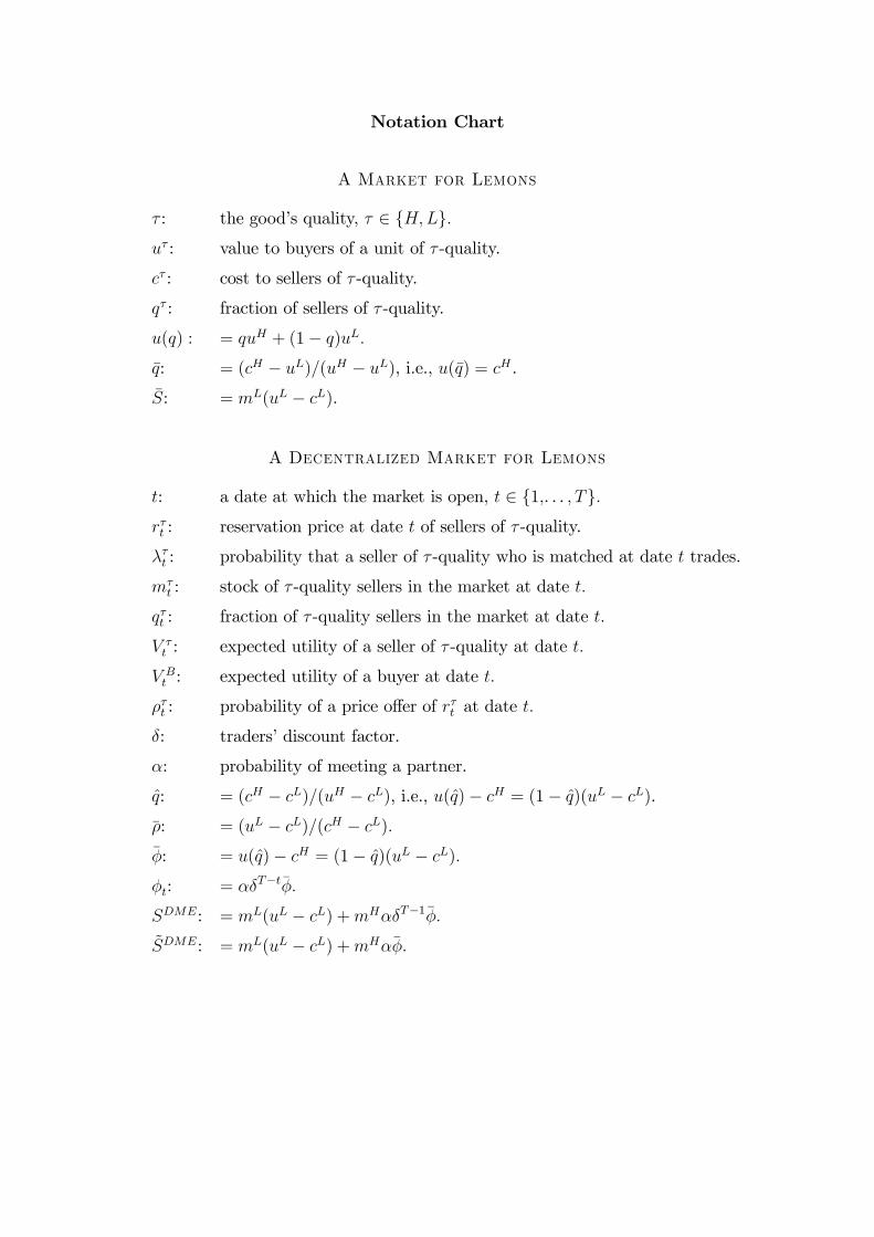
Notation Chart

A Market for Lemons

! : the goodís quality, ! 2 fH;Lg:

u! : value to buyers of a unit of ! -quality.

c! : cost to sellers of ! -quality.

q! : fraction of sellers of ! -quality.

u(q) : = quH + (1' q)uL:

'q: = (cH ' uL)=(uH ' uL), i.e., u('q) = cH .'S: = mL(uL ' cL).

A Decentralized Market for Lemons

t: a date at which the market is open, t 2 f1;. . . ; Tg:

r!t : reservation price at date t of sellers of ! -quality.

/!t : probability that a seller of ! -quality who is matched at date t trades.

m!t : stock of ! -quality sellers in the market at date t:

q!t : fraction of ! -quality sellers in the market at date t:

V !t : expected utility of a seller of ! -quality at date t:

V Bt : expected utility of a buyer at date t:

1!t : probability of a price o§er of r!t at date t:

2: tradersí discount factor.

3: probability of meeting a partner.

q: = (cH ' cL)=(uH ' cL), i.e., u(q)' cH = (1' q)(uL ' cL).

'1: = (uL ' cL)=(cH ' cL):'4: = u(q)' cH = (1' q)(uL ' cL):

4t: = 32T!t'4:

SDME: = mL(uL ' cL) +mH32T!1'4:

~SDME: = mL(uL ' cL) +mH3'4:

1 Introduction

Adverse selection pervades markets for real goods (e.g., cars, housing, labor) and

Önancial assets (e.g., insurance, stocks). Akerlofís Önding that competitive markets

for lemons may perform poorly thus has broad welfare implications, and calls for

research on fundamental questions that remain open: How do dynamic markets for

lemons perform? What is the role of frictions in alleviating adverse selection? What

determines market liquidity? Is there a role for government intervention? Our analy-

sis provides answers to these questions.

We study the performance of decentralized markets for lemons in which trade

is bilateral and time consuming, and buyers and sellers bargain over prices. These

features are common in markets for real goods and Önancial assets. We character-

ize the unique decentralized market equilibrium, identify the dynamics of transaction

prices, trading patterns, and the market composition (i.e., the fractions of units of the

di§erent qualities in the market), and study its asymptotic properties as traders be-

come perfectly patient. Using our characterization of market equilibrium, we identify

policy interventions that are welfare improving.

We consider markets in which sellers are privately informed about the quality of

the good they hold, which may be high or low, and buyers are homogeneous and

value each quality more highly than sellers. Since we are interested in understanding

dynamic trading when the lemons problem is severe, we assume that the expected

value to buyers of a random unit is below the cost of a high quality unit.1 The market

operates over a number of consecutive dates. All buyers and sellers are present at

the market open, and there is no further entry. At each date a fraction of the buyers

and sellers remaining in the market are randomly paired. In every pair, the buyer

makes a take-it-or-leave-it price o§er. If the seller accepts, then the agents trade at

that price and exit the market. If the seller rejects the o§er, then the agents split and

both remain in the market at the next date. There are trading frictions since meeting

a partner is time-consuming and traders discount future gains.

1Under this assumption, in the unique static competitive equilibrium is ine¢cient as only low

quality trades, and the entire surplus is captured by low quality sellers. We take the payo§s and

surplus at this static competitive equilibrium as the competitive benchmark. (We study dynamic

competitive equilibrium in Appendix B.)

1

In this market, equilibrium dynamics are non-stationary and involve a delicate

balance: At each date, buyersí price o§ers must be optimal given the sellersí reser-

vation prices, the market composition, and the buyersí payo§ to remaining in the

market. While the market composition is determined by past price o§ers, the sellersí

reservation prices are determined by future price o§ers. Thus, a market equilibrium

cannot be computed recursively.

We begin by studying the equilibria of decentralized markets that open over a

Önite horizon. Perishable goods such as fresh fruit or event tickets, as well as Önancial

assets such as (put or call) options or thirty-year bonds are noteworthy examples. We

show that if frictions are not large, then equilibrium is unique, and we calculate it

explicitly. The key features of equilibrium dynamics are as follows: at the Örst date,

both a low price (accepted only by low quality sellers) and negligible prices (rejected

by both types of sellers) are o§ered; at the last date, both a high price (accepted by

both types of sellers) and a low price are o§ered; and at all the intervening dates,

all three types of prices ñ high, low and negligible ñ are o§ered. Interestingly, as the

tradersí discount factor approaches one, there is trade only at the Örst and last two

dates, and the market is completely illiquid at all intervening dates.

In contrast to the competitive equilibrium, low quality trades with delay and high

quality trades. The surplus realized in the decentralized market equilibrium exceeds

the surplus realized in the competitive equilibrium: as we show, the gain realized

from trading high quality units more than o§sets the loss resulting from trading low

quality units with delay. The surplus realized increases as frictions decrease, and thus

decentralized markets yield more than the competitive surplus (and tradersí payo§s

are not competitive) even in the limit as frictions vanish.

In markets that open over an inÖnite horizon, there are multiple equilibria. We

focus on the unique equilibrium that is obtained as the market horizon approaches

inÖnity. In this equilibrium the trading dynamics are simple: at the Örst date buyers

make low and negligible price o§ers (hence only some low quality sellers trade), and at

every date thereafter buyers make only high and negligible price o§ers in proportions

that do not change over time. In contrast to prior results in the literature, each

trader obtains his competitive payo§ and the competitive surplus is realized even

when frictions are signiÖcant. Moreover, all units trade eventually, and therefore the

2

surplus lost due to trading low quality with delay exactly equals the surplus realized

from trading high quality.

Our characterization of decentralized market equilibrium yields insights into the

e§ectiveness of policies designed to increase market e¢ciency and market liquidity.

We take the liquidity of a good to be the ease with which it is sold, i.e., the equilibrium

probability it trades. In markets that open over a Önite horizon, the liquidity of high

quality decreases as traders become more patient and, somewhat counter-intuitively,

as the probability of meeting a partner increases. Indeed, as the discount factor

approaches one, trade freezes at all but the Örst and the last two dates. In markets

that open over an inÖnite horizon, the liquidity of each quality decreases as traders

become more patient, and is una§ected by the probability of meeting a partner.

We examine the impact on the market equilibrium of a variety of policies. Taxes

and subsidies conditional on the quality of the good may alleviate or aggravate the

adverse selection problem. When the horizon is Önite, providing a subsidy to buyers

or sellers of low quality raises the (net) surplus, although a subsidy to buyers has a

greater impact. In contrast, a subsidy to either buyers or sellers of high quality tends

to reduce the net surplus ñ it does so unambiguously when traders are su¢ciently

patient. Regarding liquidity, a subsidy to buyers or sellers of low quality increases the

liquidity of high quality, whereas a subsidy to buyers of high quality has the opposite

e§ect. Remarkably, when the horizon is inÖnite, a tax on high quality raises revenue

without a§ecting either payo§s or surplus, and hence increases the net surplus.

We also study subsidies conditional on the price at which the good trades. We

show that a subsidy conditional on trading at a low price increases the tradersí payo§s

as well as the net surplus. When the horizon is inÖnite the subsidy increases the

liquidity of both qualities after the Örst date, as well as the net surplus. A subsidy

conditional on trading at the high price increases (decreases) the payo§s of buyers

(low quality sellers). Interestingly, the liquidity of high quality decreases. When the

horizon is inÖnite, a subsidy is purely wasteful, whereas a tax raises revenue without

a§ecting payo§s, thus raising the net surplus.

In our setting, a Public-Private Investment Program (PPIP) such as the one im-

plemented for legacy assets is e§ectively a subsidy to buyers who purchase a low

quality unit at the high price. We show that a PPIP has e§ects analogous to sub-

3

sidizing buyers of high quality: it increases the payo§ of buyers and the surplus,

decreases the payo§ of low quality sellers and the liquidity of high quality, and as 2

approaches one reduces the net surplus.

We study the e§ect of closing the market for some period of time. Such policies

have been studied in the literature ñ e.g., Fuchs and Skrzypacz (2013) study it in a

dynamic competitive setting. Our characterization of the market equilibrium shows

that reducing the horizon over which the market opens (so long as the market remains

open for at least two dates) increases payo§s and surplus. We show that if the horizon

is not too long relative to the tradersí discount factor, then closing the market at all

dates except the Örst and the last has no e§ect on payo§s and surplus. If the horizon

is long, however, by closing the market for some period of time separating market

equilibria emerge in which the surplus is larger than when the market is open at all

dates.

Finally, we show that government purchases increase the payo§ of low quality

sellers and decrease the payo§ of buyers; surplus increases provided the government

values low quality nearly as highly as buyers, but decreases otherwise.

Related Literature

The recent Önancial crisis has stimulated interest in understanding the e§ects of

adverse selection in decentralized markets. Moreno and Wooders (2010) studies mar-

kets with stationary entry and shows that payo§s are competitive as frictions vanish.

In their setting, and in the present paper, traders only observe their own personal

histories. Kim (2011) studies a continuous time version of the model of Moreno

and Wooders (2010), and shows that if frictions are small and buyers observe the

amount of time that sellers have been in the market, then market e¢ciency improves,

whereas if buyers observe the number of prior o§ers sellers have rejected, then e¢-

ciency is reduced. Thus, Kim (2011)ís results reveal that increased transparency is

not necessarily e¢ciency enhancing, and call for caution when regulating information

disclosure. Bilancini and Boncinelli (2011) study a market for lemons with Önitely

many buyers and sellers, and show that if the number of sellers in the market is public

information, then in equilibrium all units trade in Önite time.

For markets with one-time entry, the focus of the present paper, Blouin (2003)

studies a market open over an inÖnite horizon in which only one of three exogenously

4

given prices may emerge from bargaining. Blouin (2003) shows that equilibrium

payo§s are not competitive even as frictions vanish. Although we address a broader

set of questions, on this issue we Önd that payo§s are competitive even when frictions

are non-negligible.

Camargo and Lester (2011) studies a model in which agentsí discount factors are

randomly drawn at each date from a distribution whose support is bounded away

from one, and buyers may make only one of two exogenously given price o§ers. It

shows that in every equilibrium both qualities trade in Önite time. Moreover, liquidity,

i.e., the fraction of buyers o§ering the high price, increases with the fraction of high

quality sellers initially in the market. In contrast, in our model the unique equilibrium

exhibits neither of these features: a positive measure of high quality remains in the

market at all times, and marginal changes in the fraction of high quality only a§ects

the liquidity of low quality at date 1. Camargo and Lester (2011) also provides a

numerical example demonstrating that a PPIP subsidy for has an ambiguous impact

on liquidity as measured by the minimum time at which the market clears (taken

over the set of all equilibria). We show that in our setting this policy decreases the

liquidity of high quality, and we are able to evaluate its welfare e§ects.

In contrast to Blouin (2003) and Camargo and Lester (2011) our model imposes

no restriction on admissible price o§ers. Moreover, equilibrium is unique and is

characterized in closed-form, which allows for a direct comparative static analysis of

the e§ect of changes in the parameters values on payo§s, social surplus, and liquidity.

The Örst paper to consider a matching model with adverse selection is Williamson

and Wright (1994), who show that money can increase welfare. Inderst and Muller

(2002) show that the lemons problem may be mitigated if sellers can sort themselves

into di§erent submarkets. Inderst (2005) studies a model where agents bargain over

contracts, and shows that separating contracts always emerge in equilibrium. Cho

and Matsui (2011) study long term relationships in markets with adverse selection

and show that unemployment and vacancy do not vanish even as search frictions

vanish. In their model, agents respond strategically to price proposals that are drawn

from a uniform distribution. Lauermann and Wolinsky (2011) explore the role of

trading rules in a search model with adverse selection, and show that information is

aggregated more e§ectively in auctions than under sequential search by an informed

5

buyer.

Our work also relates to a literature that examines the mini-micro foundations

of competitive equilibrium. This literature has established that decentralized trade

of homogeneous goods tends to yield competitive outcomes when trading frictions

vanish. See, for example, Gale (1987, 1996) or Binmore and Herrero (1988) when

bargaining is under complete information, and Moreno and Wooders (2002) and Ser-

rano (2002) when bargaining is under incomplete information.

There is also a growing literature studying dynamic competitive (centralized) mar-

kets with adverse selection. Janssen and Roy (2002) study a market that operates in

discrete time and in which there is a continuum of qualities, and show that competi-

tive equilibria may involve intermediate dates without trade before the market clears

in Önite time. Fuchs and Skrzypacz (2013) study a market that operates in contin-

uous time, and show that interrupting trade always raises surplus, while infrequent

trade generates more surplus under some conditions. Philippon and Skreta (2012)

and Tirole (2012) examine optimal government interventions in asset markets. In

Appendix B we study the properties of dynamic competitive equilibria in our setting,

compare the performance of centralized and decentralized markets, and discuss the

di§erential e§ects of policy interventions.

2 A Decentralized Market for Lemons

Consider a market for an indivisible commodity whose quality can be either high (H)

or low (L). There is a positive measure of buyers and sellers. The measure of sellers

with a unit of quality ! 2 fH;Lg is m! > 0. For simplicity, we assume that the

measure of buyers (mB) is equal to the measure of sellers, i.e., mB = mH + mL.2

Each buyer wants to purchase a single unit of the good. Each seller owns a single

unit of the good. A seller knows the quality of his good, but quality is unobservable

to buyers prior to purchase.

Preferences are characterized by values and costs: the value to a buyer of a unit

2This assumption is standard in the literature, e.g., it is made in all the related papers discussed

in the Introduction. It simpliÖes the analysis (without it the matching probability is endogenous

and varies over time), but involves some loss of generality.

6

of high (low) quality is uH (uL); the cost to a seller of a unit of high (low) quality is

cH (cL). Thus, if a buyer and a seller trade at price p; the buyer obtains a utility of

u ' p and the seller obtains a utility of p ' c, where u = uH and c = cH if the unit

traded is of high quality, and u = uL and c = cL if it is of low quality. A buyer or

seller who does not trade obtains a utility of zero.

We assume that both buyers and sellers value high quality more than low quality

(i.e., uH > uL and cH > cL), and that buyers value each quality more highly than

sellers (i.e., uH > cH and uL > cL). Also we restrict attention to markets in which the

lemons problem is severe; that is, we assume that the fraction of sellers of ! -quality

in the market, denoted by

q! :=m!

mH +mL;

is such that the expected value to a buyer of a randomly selected unit of the good,

given by

u(qH) := qHuH + (1' qH)uL,

is below the cost of high quality, cH . Equivalently, we may state this assumption as

qH < 'q :=cH ' uL

uH ' uL:

Note that qH < 'q implies cH > uL.

Therefore, we assume throughout that uH > cH > uL > cL and qH < 'q. Under

these parameter restrictions only low quality trades in the unique static competitive

equilibrium, even though there are gains to trade for both qualities. For future

reference, we describe this equilibrium in Remark 1 below.

Remark 1. The market has a unique static competitive equilibrium. In equilibrium

all low quality units trade at the price uL, and no high quality unit trades. Thus, the

surplus, given by

'S = mL(uL ' cL); (1)

is captured by low quality sellers.

In our model of decentralized trade, the market is open for T consecutive dates.

All traders are present at the market open, and there is no further entry. Traders

discount utility at a common rate 2 2 (0; 1], i.e., if at date t a unit of quality ! trades

7

at price p, then the buyer obtains a utility of 2t!1(u! ' p) and the seller obtains

a utility of 2t!1(p ' c! ). At each date every buyer (seller) in the market meets a

randomly selected seller (buyer) with probability 3 2 (0; 1]. In each pair, the buyer

o§ers a price at which to trade. If the o§er is accepted by the seller, then the agents

trade and both leave the market. If the o§er is rejected by the seller, then the agents

split and both remain in the market at the next date. A trader who is unmatched

at the current date also remains in the market at the next date. An agent observes

only the outcomes of his own matches.

In this market, the behavior of buyers at each date t may be described by a c.d.f.

/t with support on R+ specifying a probability distribution over price o§ers. Likewise,

the behavior of sellers of each quality is described by a probability distribution with

support on R+ specifying their reservation prices. Given a sequence / = (/1; : : : ; /T )

describing buyersí price o§ers, the maximum expected utility of a seller of quality

! 2 fH;Lg at date t 2 f1; :::; Tg is deÖned recursively as

V !t = maxx2R+

!3

Z 1

x

(p' c! ) d/t(p) +#1' 3

Z 1

x

d/t(p)

$2V !t+1

%;

where V !T+1 = 0. In this expression, the payo§ to a seller of quality ! who receives

a price o§er p is p ' c! if p is at least his reservation price x, and it is 2V !t+1; his

continuation utility, otherwise. Since all sellers of quality ! have the same maximum

expected utility, then their equilibrium reservation prices are identical. Therefore we

restrict attention to strategy distributions in which all sellers of quality ! 2 fH;Lg

use the same sequence of reservation prices r! = (r!1 ; :::; r!T ) 2 RT+.

Let (/; rH ; rL) be a strategy distribution. For t 2 f1; : : : ; Tg; the probability that

a matched seller of quality ! 2 fH;Lg trades, denoted by /!t , is

/!t =

Z 1

r!t

d/t(p): (2)

The stock of sellers of quality ! in the market at date t+ 1; denoted by m!t+1, is

m!t+1 = (1' 3/

!t )m

!t ;

wherem!1 = m

! : The fraction of sellers of high quality in the market at date t, denoted

by qHt , is

qHt =mHt

mHt +m

Lt

8

if mHt +m

Lt > 0; and q

Ht 2 [0; 1] is arbitrary otherwise.3 The fraction of sellers of low

quality in the market at date t, denoted by qLt , is

qLt = 1' qHt :

The maximum expected utility of a buyer at date t 2 f1; :::; Tg is deÖned recursively

as

V Bt = maxx2R+

8<

:3X

!2fH;Lg

q!t I(x; r!t )(u

! ' x) +

0

@1' 3X

!2fH;Lg

q!t I(x; r!t )

1

A 2V Bt+1

9=

; ;

where V BT+1 = 0. Here I(x; y) is the indicator function whose value is 1 if x ( y; and

0 otherwise. In this expression, the payo§ to a buyer who o§ers the price x is u! ' x

when matched to a ! -quality seller who accepts the o§er (i.e., when I(x; r!t ) = 1),

and it is 2V Bt+1, her continuation utility, otherwise.

DeÖnition. A strategy distribution (/; rH ; rL) is a decentralized market equilibrium

(DME) if for each t 2 f1; : : : ; Tg:

r!t ' c! = 2V !t+1 (DME:!)

for ! 2 fH;Lg; and for almost all p in the support of /t

3X

!2fH;Lg

q!t I(p; r!t )(u

! ' p) +

0

@1' 3X

!2fH;Lg

q!t I(p; r!t )

1

A 2V Bt+1 = V Bt : (DME:B)

Condition DME:! ensures that each type ! seller is indi§erent between accepting

or rejecting an o§er of his reservation price. Condition DME:B ensures that price

o§ers that are made with positive probability are optimal.

The surplus realized in a decentralized market equilibrium can be calculated as

SDME = mBV B1 +mHV H1 +mLV L1 . (3)

3Evaluating payo§s requires specifying a value for qHt for all t. Lemma 2, part 1, implies that

mHt > 0 for all t; and thus how q

Ht is speciÖed when mH

t +mLt = 0 does not a§ect equilibrium.

9

3 Decentralized Market Equilibrium

Proposition 1 establishes basic properties of decentralized market equilibria.

Proposition 1. Assume that T <1 and 2 < 1, and let t 2 f1; :::; Tg: In a DME :

(P1.1) rHt = cH > rLt , V

Ht = 0, and qHt+1 ( qHt .

(P1.2) Only the high price pt = rHt , or the low price pt = rLt ; or negligible prices

pt < rLt may be o§ered with positive probability.

The intuition for these results is straightforward. Since the payo§ of a seller who

does not trade at date T is zero, sellersí reservation prices at date T are equal to

their costs, i.e., r!T = c! . Thus, price o§ers above cH are suboptimal at date T , and

are made with probability zero. Therefore the expected utility of high quality sellers

at date T is zero, i.e., V HT = 0; and hence rHT!1 = cH : Also, since 2 < 1, i.e., delay

is costly, low quality sellers accept price o§ers below cH ; i.e., rLT!1 < cH . A simple

induction argument shows that rHt = cH > rLt for all t.

Obviously, prices above rHt , which are accepted by both types of sellers, or prices in

the interval (rLt ; rHt ), which are accepted only by low quality sellers, are suboptimal,

and are therefore made with probability zero. Moreover, since rHt > rLt then the

proportion of high quality sellers in the market (weakly) increases over time (i.e.,

qHt+1 ( qHt ) as low quality sellers accept o§ers of both rHt and rLt , and therefore exit

the market at least as fast as high quality sellers, who only accept o§ers of rHt .

In equilibrium, at each date a buyer may o§er a high price p = rHt , which is

accepted by both types of sellers, or a low price p = rLt , which is accepted by low

quality sellers and rejected by high quality sellers, or a negligible price p < rLt ; which

is rejected by both types of sellers. For ! 2 fH;Lg denote by 1!t the probability of a

price o§er equal to r!t : Since prices greater than rHt are o§ered with probability zero,

then the probability of a high price o§er is 1Ht = /Ht . (Recall that /

!t is the probability

that a matched ! -quality seller trades at date t ñ see equation (2).) And since prices

in the interval (rLt ; rHt ) are o§ered with probability zero, then the probability of a

low price o§er is 1Lt = /Lt ' /Ht : Thus, the probability of a negligible price o§er is

1' (1Ht + 1Lt ) = 1' /Lt .

Proposition 1 thus allows a simpler description of a DME. Henceforth we describe

a DME by a collection (1H ; 1L; rL), where 1! = (1!1; : : : ; 1!T ) for ! 2 fH;Lg, and thus

10

ignore the distribution of negligible price o§ers, which is inconsequential. Also we

omit the reservation price of high quality sellers which is rHt = cH for all t by P1:1.

Proposition 2 establishes additional properties of DME.

Proposition 2. Assume that T <1 and 2 < 1. Then in a DME:

(P2.1) At every date t 2 f1; : : : ; Tg either high or low prices are o§ered with positive

probability, i.e., 1Ht + 1Lt > 0.

(P2.2) At date 1 high prices are o§ered with probability zero, i.e., 1H1 = 0:

(P2.3) At date T negligible prices are o§ered with probability zero, i.e., 1'1HT '1LT = 0.

The intuition for P2:2 is clear: Since at date 1 the expected utility of a random

unit is less than cH by assumption, then high price o§ers are suboptimal, i.e., 1H1 = 0.

The intuition for P2:3 is also simple: At date T the sellersí reservation prices are equal

to their costs. Thus, buyers obtain a positive payo§ by o§ering either the low price

rLT = cL (when qHT < 1), or the high price rHT = cH (when qHT = 1). Since a buyer

who does not trade obtains zero, then negligible price o§ers are suboptimal, i.e.,

1HT + 1LT = 1. The intuition for P2:1 is as follows: Suppose to the contrary that

all buyers make negligible o§ers at date t, i.e., 1Ht = 1Lt = 0: Let t0 be the Örst

date following t where a buyer makes a non-negligible price o§er. Since there is no

trade between t and t0, then the distribution of qualities is the same at t and t0; i.e.,

qHt = qHt0 . Thus, an impatient buyer is better o§ by o§ering at date t the price she

o§ers at t0; which implies that negligible prices are suboptimal at t; i.e., 1Ht + 1Lt = 1:

Hence 1Ht > 0 and/or 1Lt > 0:

In a market that opens for a single date, i.e., T = 1, the sellersí reservation prices

are their costs. The fraction of high quality sellers

q :=cH ' cL

uH ' cL;

makes a buyer indi§erent between an o§er of cH and an o§er of cL. It is easy to see

that 'q < q: Since qH < 'q by assumption, then qH < q. Thus, if T = 1 only low price

o§ers are made (i.e., 1H1 = 0 and 1L1 = 1) and only low quality trades, as implied by

P2:1 and P2:2. Remark 2 states these results.

Remark 2. Assume that T = 1 and 2 < 1. Then the unique DME is (1H1 ; 1L1 ; r

L1 ) =

(0; 1; cL). In equilibrium some low quality units trade at the price cL, and no high

11

quality unit trades. Thus, the surplus realized, which is 3mL(uL' cL), is captured by

buyers.

Proposition 3 below establishes that when frictions are not large a decentralized

market that opens over a Önite horizon T > 1 has a unique DME.We say that frictions

are not large when 3 and 2 are su¢ciently near one that the following inequalities

hold:'1

32< min

!cH ' uL

(1 + 32) (1' 2) (cH ' cL); 1

%; (F:1)

and(1' '1=2)qH

(1' '1=2)qH + (1' 3)(1' qH)> q; (F:2)

where

'1 :=uL ' cL

cH ' cL:

Inequality F:1 requires 3 and 2 be su¢ciently close to one that a low quality seller

prefers to wait one period and trade with probability 3 at the price cH rather than

trading immediately at the price uL. The left hand side of F:1, '1=32, is an upper

bound of the probability that a high price is o§ered at any date as we show in Lemma

2, part 6, in the Online Appendix. It is easy to see that F:1 holds for 3 and 2 near

one.

Inequality F:2 requires that if all matched low quality sellers trade and at most a

fraction '1=32 of matched high quality sellers trade, then the fraction of high quality

sellers in the market at the next date is above q: In Lemma 2, part 2, in the Online

Appendix we show that this inequality implies that the low price is never o§ered with

probability one. Obviously, this inequality holds for 3 near one.

Write

'4 := (1' q)(uL ' cL);

and for t 2 f1; : : : ; Tg let

4t = 32T!t'4:

Clearly 4t is increasing in 3 and 2; and approaches 3'4 as 2 approaches one; and 4t

is decreasing in T; and approaches zero as T approaches inÖnity.

Proposition 3 establishes that when frictions are not large a market that opens

over a Önite horizon has a unique DME, and provides a complete characterization of

this equilibrium.

12

Proposition 3. Assume that 1 < T <1, 2 < 1; and inequalities F:1 and F:2 hold

(i.e., frictions are not large). Then the unique DME is given by:

(P3.1) High Price O§ers: 1H1 = 0,

1Ht =1' 232

uL ' cL

cH ' uL + 4t

for all 1 < t < T , and

1HT =uL ' cL ' 32'432(cH ' cL)

:

(P3.2) Low Price O§ers:

1L1 =42 + c

H ' u(qH)3(1' qH)(cH ' uL + 42)

;

and 1LT = 1' 1HT . If T > 2, then

1Lt = (1' 31Ht )

(1' 2)4t+131cH ' uL + 4t+1

2 uH ' uL

uH ' cH ' 4t

for all 1 < t < T ' 1, and

1LT!1 = (1' 31HT!1)

(1' 32)(u(q)' cH)3q(uH ' cH ' 4T!1)

:

(P3.3) Reservation Prices: rLt = uL ' 4t for all t < T , and rLT = cL:

In equilibrium, the payo§ to a buyer is V B1 = 41, and the payo§s to sellers are

V H1 = 0 and V L1 = uL ' cL ' 41. Thus, the payo§ to a buyer (low quality seller)

is above (below) his competitive payo§, decreases (increases) with T and increases

(decreases) with 3 and 2. Moreover, the surplus, given by

SDME = mL(uL ' cL) +mH32T!1'4,

is above the competitive surplus 'S, decreases with T , and increases with 3 and 2.

It is easy to describe the equilibrium trading patterns: at the Örst date only low

and negligible prices are o§ered, and thus some low quality sellers trade, but no high

quality seller trades (i.e., 1H1 = 0 < 1L1 < 1). At intermediate dates, high, low and

negligible prices are o§ered (i.e., 1Ht ; 1Lt > 0 and 1 ' 1Ht ' 1Lt > 0), and thus some

sellers of both types trade. At the last date only high and low prices are o§ered (i.e.,

1HT + 1LT = 1 ), and thus all matched low quality sellers and some high quality sellers

trade.

13

Thus, both qualities trade with delay. Nevertheless, the surplus generated in the

DME is greater than the competitive equilibrium surplus, 'S: the gain from trading

high quality units more than o§sets the loss from trading low quality units with delay.

In contrast, in a market for a homogenous good the competitive equilibrium surplus

is an upper bound to the surplus that can be realized in a DME ñ e.g., Moreno and

Wooders (2002) show that this bound is achieved as frictions vanish.

Price dispersion is a key feature of equilibrium: At every date but the Örst there is

trade at more than one price since both high and low prices are o§ered with positive

probability. To see that price dispersion is essential, suppose instead that the high

price cH is o§ered with probability one at some date t. Since 3 and 2 are near one,

this implies that the reservation price of low quality sellers prior to t is near cH ,

and hence above the value of low quality uL (recall that uL < cH). Thus, prior to

t a low price o§er (which if accepted buys a unit of low quality) is suboptimal, and

therefore low price o§ers are made with probability zero. Therefore sellers of both

qualities leave the market at the same rate, and hence the fraction of high quality

sellers remains constant, i.e., qHt = qH . Since qH < 'q; a high price o§er is suboptimal

at t, which is a contradiction. Hence high price o§ers are made with probability less

than one at every date.

Likewise, suppose that the low price is o§ered with probability one at some date t.

Then at date t all matched low quality sellers trade, and no high quality seller trades.

Since 3 is near one, this implies that the fraction of high quality sellers in the market

at date t + 1 is near one, and since this sequence in non-decreasing over time, the

fraction of high quality sellers at the last date is above q. (Recall that q is the fraction

of high quality sellers that makes buyers indi§erent between o§ering the high and the

low price at date T .) This implies that o§ering cH is uniquely optimal and hence the

high price is o§ered with probability one at date T; which is a contradiction. Thus,

low price o§ers are made with probability less than one at every date.

A more involved argument establishes that all three types of price o§ers (high,

low, and negligible) are made with positive probability at every date except the Örst

and last ñ see the proof of Lemma 2, part 7, in the Online Appendix.

Identifying the probabilities (1Ht ; 1Lt ) is delicate: Their past values determine the

current market composition, qHt , and their future values determine the reservation

14

price of low quality sellers at date t. In equilibrium, at intermediate dates the market

composition and the sellersí reservation prices must make buyers indi§erent between

o§ering high, low or negligible prices, i.e., the equation

u(qHt )' cH = (1' qHt )(u

L ' rLt ) + qHt 2V

Bt+1 = 2V

Bt+1

holds. We show in the proof of Proposition 3 in Appendix A that the system formed

by these equations (together with the analogous equations for dates 1 and T , and the

boundary conditions) admits a single solution. Establishing uniqueness of equilibrium

requires showing that these properties are common to all market equilibria ñ see

Lemma 2 in the Online Appendix.

The comparative static properties of equilibrium relative to 3; 2 and T are intu-

itive: Since negligible price o§ers are optimal at every date except the last, the payo§

to buyers is just their discounted payo§ at the last date. Consequently, the payo§ to

a buyer increases with 3 and 2, and decreases with T . Low quality sellers capture

surplus whenever high price o§ers are made, i.e., at every date except the Örst. The

probability of a high price o§er decreases with both 3 and 2, and increases with T ,

and thus the payo§ to low quality sellers decreases with 3 and 2, and increases with

T . The surplus increases with 3 and 2.

Somewhat counter-intuitively, the surplus decreases with T , i.e., shortening the

horizon over which the market opens is advantageous (so long as T > 2): Our as-

sumption that frictions are small implies that in equilibrium buyers must be willing

to o§er negligible prices at every date but the last date. Hence their payo§ is just

their discounted expected utility at the last date.4 Thus, a longer horizon provides

no advantage in screening sellers, and reduces the buyersí payo§. The payo§ to low

quality sellers increases with T because the high price is o§erred with higher proba-

bility at every date (except at the last date, at which it is o§erred with a probability

independent of T ). Further, since buyersí must remain willing to o§er the low price,

the increase in the payo§ of low quality sellers exactly matches the decrease in the

payo§ of buyers. Therefore the surplus decreases with T since there are more buyers

than low quality sellers, and is maximal when T = 2.4In contrast, if traders are su¢ciently impatient, then there is an equilibrium in which buyers

o§er rL1 at date 1, and then o§er cH at every subsequent date. In this equilibrium, lengthening the

horizon increases surplus when ( < 1.

15

A striking feature of equilibrium in decentralized markets is that the surplus

realized exceeds the competitive equilibrium surplus: decentralized markets are more

e¢cient than centralized ones. While in a centralized market all units trade at a single

market-clearing price, in a decentralized market several prices are o§ered with positive

probability, and di§erent units trade at di§erent prices. When 3 = 1, for example,

low quality units trade for sure ñ some at the high price and some at the low price

ñ while high quality units trade with probability less than one. Thus decentralized

trade generates an allocation closer to the surplus maximizing allocation, in which low

quality sellers trade for sure, and high quality sellers trade with positive probability

(less than one).5

Proposition 4 identiÖes the limiting DME as traders become perfectly patient. A

remarkable feature of the limiting equilibrium is that the market freezes at interme-

diate dates, and both qualities are completely illiquid: Low quality trades at the Örst

and last two dates, and high quality trades only at the last date. The surplus is

independent of the duration of the market.

Proposition 4. Assume that 1 < T <1, 2 < 1, and inequalities F:1 and F:2 hold

(i.e., frictions are not large). Then as 2 approaches one the unique DME approaches

(~1H ; ~1L; ~rL) given by:

(P4.1) High Price O§ers: ~1Ht = 0 for all t < T , and

~1HT =uL ' cL ' 3'43(cH ' cL)

.

(P4.2) Low Price O§ers:

~1L1 =3'4+ cH ' u(qH)

3(1' qH)(cH ' uL + 3'4);

and ~1LT = 1' ~1HT : If T > 2, then ~1

Lt = 0 for all 1 < t < T ' 1 and

~1LT!1 =(1' 3)(u(q)' cH)3q(uH ' cH ' 3'4)

:

5The (static) surplus maximizing menu contract is f(pH ; ZH); (pL; ZL)g, where pH = cH , ZH =

(1 ' qH)(uL ' cL)=[cH ' cL ' qH(uH ' cL)], pL = cL + ZH(cH ' cL) and ZL = 1. Here p$ is the

money transfer from seller to buyer and Z$ is the probability that the seller transfers the unit of

good to the buyer, when the seller reports type . . Even if ( = 1, in the DME high quality sellers

trade with probability less than ZH .

16

(P4.3) Reservation Prices: ~rLt = uL ' 3'4 for all t < T , and ~rLT = cL:

Moreover, (~1H ; ~1L; ~rH ; ~rL) is a DME of the market when 2 = 1. In equilibrium, the

payo§ to a buyer is ~V B1 = 3'4, and the payo§s to sellers are ~V H1 = 0 and ~V L1 =

[1 ' 3 (1' q)](uL ' cL). Thus, the payo§ to a buyer (low quality seller) remains

above (below) his competitive payo§. The surplus, given by

~SDME = mL(uL ' cL) +mH3'4;

is independent of T and remains above the competitive surplus.

When 2 = 1, time can no longer be used as a screening device (until the very last

period), and the market freezes at all dates but the last two. The DME identiÖed

in Proposition 4 is not the unique market equilibrium. For example, there are DME

in which buyers mix over low and negligible prices at dates prior to T in such a way

that the total measure of low quality sellers that trades prior to T is the same as in

the DME identiÖed in Proposition 4; then buyers o§er high and low prices at date T

with probabilities ~1HT and ~1LT , respectively.

We illustrate our Öndings in propositions 3 and 4 with an example.

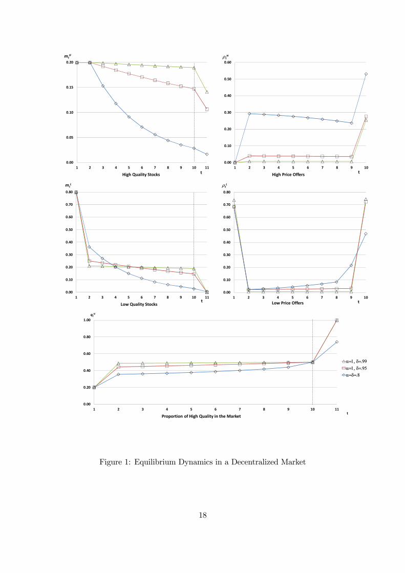
Example 1

Consider a market in which uH = 1, cH = :6, uL = :4, cL = :2, mH = :2, mL = :8,

and T = 10. The graphs in the top row of Figure 1 show the evolution of the stocks

of high quality sellers mHt in the market, and the fraction of high price o§ers 1Ht

for several di§erent combinations of 3 and 2. The graphs in the middle row show

the evolution of mLt and 1

Lt . The bottom graph shows the evolution of the fraction

of high quality sellers in the market qHt . These graphs illustrate several features of

equilibrium as frictions become small: high quality trades more slowly; low quality

trades more quickly at the Örst date and at the last date, but trades more slowly at

intermediate dates; the fraction qHt increases more quickly, but equals q = :5 at the

market close regardless of the level of frictions.

17

0.00

0.05

0.10

0.15

0.20

1 2 3 4 5 6 7 8 9 10 11

mtH

tHigh�Quality�Stocks

0.00

0.20

0.40

0.60

0.80

1.00

1 2 3 4 5 6 7 8 9 10 11

qtH

tProportion�of�High�Quality�in�the�Market

D ���G ���D ���G ���D G ��

0.00

0.10

0.20

0.30

0.40

0.50

0.60

0.70

0.80

1 2 3 4 5 6 7 8 9 10 11

mtL

tLow�Quality�Stocks

0.00

0.10

0.20

0.30

0.40

0.50

0.60

1 2 3 4 5 6 7 8 9 10

UtH

tHigh�Price�Offers�

0.00

0.10

0.20

0.30

0.40

0.50

0.60

0.70

0.80

1 2 3 4 5 6 7 8 9 10

UtL

tLow�Price�Offers�

Figure 1: Equilibrium Dynamics in a Decentralized Market

18

Decentralized Market Equilibria when the Horizon is Infinite

We now consider decentralized markets that open over an inÖnite horizon. In these

markets, given a strategy distribution one calculates the maximum expected utility

of each type of trader at each date by solving a dynamic optimization problem. The

deÖnition of DME remains otherwise the same.

Proposition 5 identiÖes the limiting DME as T approaches inÖnity, and establishes

it this limit is a DME of the market that opens over an inÖnite horizon. In relating

the formulae in propositions 3 and 5, it is useful to observe that 4t approaches zero

as T approaches inÖnity.

Proposition 5. Assume that 2 < 1; and inequalities F:1 and F:2 hold (i.e., frictions

are not large). Then as T approaches inÖnity the unique DME approaches (1H ; 1L; rL)

given by:

(P5.1) High Price O§ers: 1H1 = 0, and for all t > 1,

1Ht =1' 232

uL ' cL

cH ' uL:

(P5.2) Low Price O§ers:

1L1 ='q ' qH

3'q (1' qH)and 1Lt = 0 for all t > 1:

(P5.3) Reservation Prices: rLt = uL for all t.

Moreover, if T = 1 then (1H ; 1L; rH ; rL) is a DME. In equilibrium, the tradersí

payo§s are the competitive payo§s, i.e., V B1 = 0; V H1 = 0 and V L1 = uL' cL, and the

surplus is the competitive surplus 'S.

As the horizon becomes inÖnite, all units trade eventually. At the Örst date,

some low quality units trade but no high quality units trade. At subsequent dates,

units of both qualities trade with the same constant probability. In the limit, the

tradersí payo§s are competitive independently of 3 and 2, and hence so is the surplus,

even if frictions are non-negligible. Kim (2011) obtains an analogous result in a

stationary setting. In contrast, the previous literature has established that payo§s are

competitive only as frictions vanish, e.g., Gale (1987), Binmore and Herrero (1988),

and Moreno and Wooders (2002) for homogenous goods markets, and Moreno and

Wooders (2010) for markets with adverse selection.

19

The intuition for these results is simple: in the DME of a market that opens over

a Önite horizon, the payo§ to a buyer at the last date is V BT = 3'4 > 0, independently

of the horizon T . Since negligible prices are optimal at every date except the last, the

payo§ to a buyer is his discounted payo§ at the last date, 32T!1'4, which approaches

zero as the horizon approaches inÖnity. Thus, in a market that opens over an inÖnite

horizon the payo§ to a buyer is zero. Hence low price o§ers, if made with positive

probability, must yield a payo§ equal to zero, which implies that rLt = uL > cL.

Then high prices must be o§ered with positive probability at some dates. At these

dates the proportion of high quality must be 'q in order for the expected payo§ to a

buyer o§ering the high price to be zero. In a stationary equilibrium, the equation

rLt = uL pins down the rate at which high price o§ers are made, and qH2 = 'q pins

down the proportion of low price o§ers at date 1. Since the payo§s of buyers is zero,

the proportion of high quality sellers in the market can not rise above 'q, and thus

low price o§ers are made with probability zero after date 1.

When T = 1 there are multiple equilibria. Uniqueness of equilibrium when the

horizon is Önite justiÖes focusing on the limiting DME identiÖed in Proposition 5.6

4 Policy Intervention

Our results allow an assessment of the impact of policies aimed at improving mar-

ket e¢ciency, such as subsidies, taxes, programs like the Public-Private Investment

Program for Legacy Assets, or other interventions like closing the market for some

period of time.

Taxes and Subsidies Conditional on Quality

Suppose that the government provides a per unit subsidy of BLB > 0 to buyers

of low quality. Then the instantaneous payo§ to a buyer who purchases a unit of

6When T =1 there is a continuum of DME that share the basic properties identiÖed in Propo-

sition 5: 0H1 = 0, 0L1 > 0 is such that q

H2 = )q, and rL1 = u

L * rLt for all t > 1. In these DME, payo§s

are competitive: V B1 = 0 implies rL1 = uL, and thus V L1 = 2V L2 = rL1 ' cL = uL ' cL. In fact, we

conjecture that payo§s are competitive in all DME. This conjecture is based on the idea that in all

DME buyers make negligible price o§ers with positive probability at every date, which implies that

their payo§ would diverge if it was positive. (Proving this conjecture requires establishing versions

of lemmas 1 and 2 for a market with T =1.)

20

low quality at price p is uL + BLB ' p rather than uL ' p. The impact of the subsidy

may therefore be evaluated as an increase in the value of low quality, uL. Likewise,

if the government provides a per unit subsidy of BLS > 0 to sellers of low quality,

then the instantaneous payo§ to a seller who sells a unit of low quality at price p is

p ' (cL ' BLS) rather than p ' cL, and therefore the impact of the subsidy may be

evaluated as a decrease in the cost of low quality, cL. Such subsidies are feasible

provided that quality is veriÖable following purchase. Taxes are negative subsidies.

When T <1, the e§ect of a subsidy on the market equilibriummay be determined

using the formulae given in Proposition 3. For example, subsidizing buyers of low

quality increases the net surplus: a marginal subsidy increases (gross) surplus by

@SDME

@uL= mL +mH32T!1

d'4

duL= mL +mH32T!1 (1' q) ;

whereas the present value of the subsidy is at most mL since at most mL units receive

the subsidy. Subsidizing sellers of low quality increases the net surplus as well since

@SDME

@cL= 'mL +mH32T!1

d'4

dcL= 'mL 'mH32T!1 (1' q)

uH ' uL

uH ' cL< 'mL:

Comparing these two expressions reveals that subsidizing buyers has a larger e§ect on

surplus, i.e., @SDME=@uL > j@SDME=@cLj, since (uH ' uL)=(uH ' cL) < 1. Corollary

1 below summarizes the e§ect of subsidies to low quality on payo§s and surplus.

Its proof, which follows from di§erentiating the formulae given in Proposition 3, is

omitted.

Corollary 1. Under the assumptions of Proposition 3, a subsidy to either buyers or

sellers of low quality increases the payo§s of buyers and low quality sellers, as well

as the net surplus. However, subsidizing buyers has a larger e§ect on the payo§ of

buyers and on the surplus SDME, and a smaller e§ect on the payo§ of low quality

sellers, than subsidizing sellers.

The intuition for the result that subsidies to low quality raise surplus is as follows:

A subsidy, whether to buyers or sellers, raises the payo§ to buyers at the last date,

V BT , and therefore raises their payo§ at every date, VBt . Consider a subsidy to buyers.

Since buyers must remain indi§erent between low and negligible price o§ers prior to

date T , i.e.,

(1' qHt )(uL ' rLt ) + q

Ht 2V

Bt+1 = 2V

Bt+1,

21

(equivalently, uL' rLt = 2V Bt+1), then the reservation price of low quality sellers must

increase.7 Hence the payo§ to low quality sellers must increase, which requires that

high price o§ers be made more frequently at every date (except the Örst). Thus, a

greater measure of high quality trades and a greater surplus is realized. A subsidy

to buyers yields a greater increase in the payo§ to buyers at the last date than does

an equal-sized subsidy to sellers, and therefore a subsidy to buyers leads to a greater

increase in surplus.

Next we describe the impact of subsidies to buyers and sellers of high quality.

When T < 1, the e§ect of such subsidies on payo§s and on the surplus may be

assessed using the formulae of Proposition 3 as changes in the value or cost of high

quality. Their impact on the net surplus is unclear in general as it is di¢cult to

calculate the present value of the subsidy, but as 2 approaches one the e§ect is clear

from Proposition 4: A subsidy to buyers of high quality a§ects surplus through its

impact on q:

@ ~SDME

@uH= 'mH3(uL ' cL)

@q

@uH= mH3(uL ' cL)

cH ' cL

(uH ' cL)2:

Since high quality trades only at the last date, the marginal cost of the subsidy

approaches mH3~1HT . Thus the marginal e§ect on the net surplus approaches

@ ~SDME

@uH'mH3~1HT = mH3(uL ' cL)

cH ' cL

(uH ' cL)2'mH u

L ' cL ' 3'4(cH ' cL)

* mH uL ' cL

uH ' cL

#cH ' cL

uH ' cL' 1$

< 0;

where the weak inequality holds since 3 * 1. A subsidy to sellers of high quality also

reduces the net surplus since

@ ~SDME

@cH= 'mH3(uL ' cL)

@q

@cH= 'mH3

uL ' cL

uH ' cL;

and therefore33333@ ~SDME

@cH

33333'mH3~1HT = '(1' 3)m

H uL ' cL

uH ' cLuH ' cL

cH ' cL* 0:

7A subsidy of 3LB increases 2VBt+1 by less than 3

LB , whereas u

L increases by 3LB . Hence rLt must

increase in order to preserve the equality.

22

We state these results in Corollary 2.

Corollary 2. Under the assumptions of Proposition 3, subsiding either buyers or

sellers of high quality has the same qualitative e§ects: the payo§ of buyers and the

surplus increase, and the payo§ of low quality sellers decreases. However, subsidizing

sellers has a larger e§ect on payo§s and surplus. As 2 approaches one, either subsidy

reduces the net surplus.

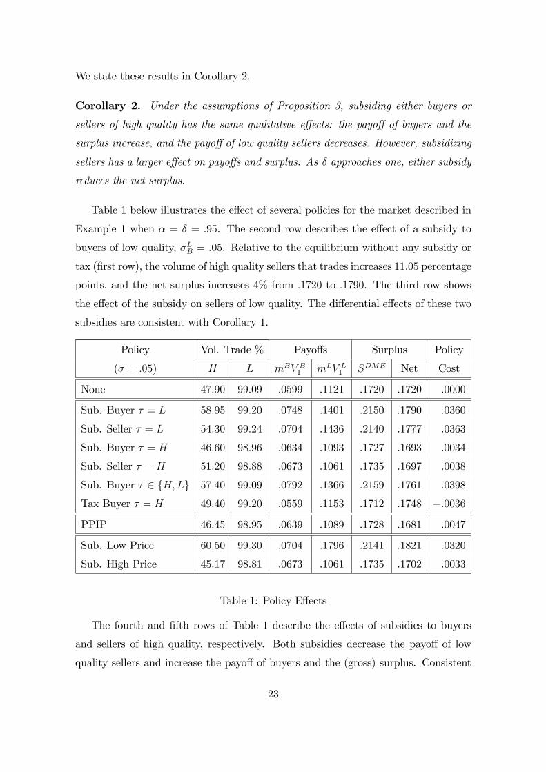
Table 1 below illustrates the e§ect of several policies for the market described in

Example 1 when 3 = 2 = :95. The second row describes the e§ect of a subsidy to

buyers of low quality, BLB = :05. Relative to the equilibrium without any subsidy or

tax (Örst row), the volume of high quality sellers that trades increases 11:05 percentage

points, and the net surplus increases 4% from :1720 to :1790. The third row shows

the e§ect of the subsidy on sellers of low quality. The di§erential e§ects of these two

subsidies are consistent with Corollary 1.

Policy Vol. Trade % Payo§s Surplus Policy

(B = :05) H L mBV B1 mLV L1 SDME Net Cost

None 47:90 99:09 .0599 .1121 .1720 .1720 .0000

Sub. Buyer ! = L 58:95 99:20 .0748 .1401 .2150 .1790 .0360

Sub. Seller ! = L 54:30 99:24 .0704 .1436 .2140 .1777 .0363

Sub. Buyer ! = H 46:60 98:96 .0634 .1093 .1727 .1693 .0034

Sub. Seller ! = H 51:20 98:88 .0673 .1061 .1735 .1697 .0038

Sub. Buyer ! 2 fH;Lg 57:40 99:09 .0792 .1366 .2159 .1761 .0398

Tax Buyer ! = H 49:40 99:20 .0559 .1153 .1712 .1748 ':0036

PPIP 46:45 98:95 .0639 .1089 .1728 .1681 .0047

Sub. Low Price 60:50 99:30 .0704 .1796 .2141 .1821 .0320

Sub. High Price 45.17 98.81 .0673 .1061 .1735 .1702 .0033

Table 1: Policy E§ects

The fourth and Öfth rows of Table 1 describe the e§ects of subsidies to buyers

and sellers of high quality, respectively. Both subsidies decrease the payo§ of low

quality sellers and increase the payo§ of buyers and the (gross) surplus. Consistent

23

with Corollary 2, these e§ects are stronger for the subsidy to sellers than the subsidy

to buyers. In the example, the negative e§ect on net surplus of the subsidy to sellers

is smaller.

The sixth row of Table 1 reports the e§ects of an unconditional subsidy to buyers.

(If quality is not veriÖable after purchase, then a subsidy conditional on the quality

of the good is not feasible.) The unconditional subsidy has a smaller positive e§ect

on the net surplus than a subsidy on buyers of low quality alone. The seventh row of

Table 1 shows the e§ect of a tax on buyers of high quality. Its e§ects are opposite of

a subsidy. In particular, it increases the measures of trade of both qualities and the

net surplus.

Next we address the e§ects of taxes and subsidies in a market that opens over an

inÖnite horizon. In such markets the e§ects of subsidies on either quality are easily

assessed by di§erentiating the formulae provided in Proposition 5. Inspecting these

formulae leads to an interesting Örst observation: in these markets subsidizing either

buyers or sellers of ! -quality has identical e§ects on payo§s and surplus. Corollary

3 describes the e§ects of subsidizing low quality.

Corollary 3. Assume that T = 1 and the assumptions of Proposition 5 hold.

Subsidizing low quality has no e§ect on the payo§ of buyers, and increases the payo§

of low quality sellers and the net surplus. As 2 approaches one, the subsidy has no

e§ect on the net surplus and amounts to a transfer to low quality sellers.

While a subsidy BL to low quality raises the surplus by BLmL, the present value of

the subsidy is less than BLmL, and therefore the net surplus increases. Establishing

that as 2 approaches one a subsidy BL to low quality amounts to a transfer to low

quality sellers requires showing that the present value of the subsidy approaches BLmL

ñ see the proof of Corollary 3 in Appendix A.

Interestingly, a tax on high quality raises revenue without a§ecting either payo§s

or surplus, thereby increasing net surplus. A tax on buyers of high quality, for

example, increases 1L1 while leaving 1Lt and 1

Ht unchanged for t > 1, thus accelerating

trade. We state this result in Corollary 4.

Corollary 4. Assume that T =1 and the assumptions of Proposition 5 hold. A tax

on high quality raises revenue without a§ecting payo§s or surplus, thereby increasing

24

the net surplus.

Market Liquidity

Liquid assets are those that can be easily bought or sold. In our setting, we deÖne

the liquidity of a good to be the equilibrium probability that it trades. In equilibrium,

at each date t high quality trades with probability 31Ht , and low quality trades with

probability 3(1Ht + 1Lt ). Since high quality is always illiquid at date 1, we focus on

its liquidity at dates t > 1.

Corollary 5 describes the e§ects on liquidity of subsidies, taxes, and market fric-

tions in a market that opens over a Önite horizon. These results, which are provided

without proof, are obtained by di§erentiating the formulae in Proposition 3. Perhaps

counter-intuitively, high quality is less liquid as the probability of meeting a part-

ner 3 increases or as traders become more patient. Indeed, both qualities become

completely illiquid at intermediate dates as 2 approaches one ñ see Proposition 4.

Corollary 5. Under the assumptions of Proposition 3 the liquidity of high quality

decreases monotonically as frictions vanish. It also increases if either buyers of low

quality or sellers of either quality are subsidized, and decreases if buyers of high quality

are subsidized.

The intuition for the e§ects of subsidies to low quality were discussed in connection

to Corollary 1. A subsidy to buyers of high quality raises the payo§s of buyers at

the last date, and therefore raises their payo§ at every date, V Bt . Since buyers

must remain indi§erent between low and rejected price o§ers prior to date T , i.e.,

uL' rLt = 2V Bt+1, and since uL is una§ected by the subsidy, then the reservation price

(and payo§) of low quality sellers must decrease. Hence high price o§ers are made

less frequently, i.e., the liquidity of high quality decreases.

The e§ects of subsidies to high quality sellers are more subtle: A subsidy BHS

raises V Bt at every date, and since it does not a§ect uL, then rLt (and VLt+1) must

decrease. At the same time, the subsidy reduces the high price o§er, which becomes

cH ' BHS , and therefore directly reduces the payo§ of low quality sellers. The e§ect

on the frequency of high price o§ers is thus ambiguous, and must be determined by

signing a derivative. It turns out this derivative is positive, i.e., the (now smaller)

25

high price o§er is made more frequently with the subsidy, and therefore the liquidity

of high quality increases.

Corollary 6 establishes results on liquidity for a market that opens over an inÖnite

horizon. These results follow from di§erentiating the formulae in Proposition 5.

These formulae reveal that the liquidity of low quality at date 1 is independent of the

discount factor, decreases with a subsidy on high quality, decreases with a subsidy to

buyers of low quality, and is una§ected by subsidies to low quality sellers. Since low

prices are o§ered only at the Örst date (i.e., 1Lt = 0 for all t > 1), the liquidity of both

qualities for t > 1 is 31Ht . Note that 31Ht is independent of 3, i.e., the liquidities of

both goods are una§ected by changes in the probability of meeting a partner 3.

Corollary 6. Assume that T = 1 and the assumptions of Proposition 5 hold.

The liquidities of both qualities at dates t > 1 approach zero monotonically as the

tradersí become perfectly patient, increase with a subsidy on low quality, decrease with

a subsidy to high quality sellers, and are una§ected by subsidies to buyers of high

quality.

The Public-Private Investment Program for Legacy Assets

This program was designed to draw new private capital into the market for trou-

bled real estate-related assets, comprised of legacy loans and securities, by providing

equity co-investment and public Önancing. Its main objective was to reduce the

perceived excessive liquidity discounts in legacy asset prices. The program provided

private investors with non-recourse loans to purchase legacy assets. Investors had to

provide only a small amount of equity (a fraction D = 1=14 of the purchase price).

Thus, under this program an investor who purchased a low quality asset may choose

to default on the loan and surrender the asset, losing only her equity (i.e., the fraction

D of the price paid for the asset).

This policy may be framed in our setting as a subsidy to buyers who pay the high

price cH for a low quality unit: under this program a buyer who purchases at the

high price, upon observing the quality of the unit acquired faces the choice to keep

the unit and pay the loan, which is optimal if it is of high quality since

uH > (1' D) cH ;

26

or default and surrender the unit, which is optimal when it is of low quality provided

uL < (1' D) cH :

Assuming that D is su¢ciently small that this inequality holds, the payo§ to a buyer

o§ering the high price cH when the fraction of high quality in the market is q; denoted

by PH ; is

PH = q1uH ' cH

2+ (1' q)

1'DcH

2:

This payo§ may be written as

PH(q; s) = quH + (1' q) uL ' cH + (1' q)s

= u(q)' cH + (1' q)s;

where s = (1'D)cH'uL is e§ectively a subsidy to buyers who purchase a low quality

unit at the high price cH :

Of course, the lemons problem can be solved altogether by setting a subsidy

su¢ciently large. Evaluating the impact of a small subsidy is somewhat more complex

than a comparative statics exercise. However, the introduction of a small PPIP

subsidy does not change the basic properties of equilibrium, and the formulae provided

in propositions 3 to 5 describing the DME can be readily modiÖed to show the impact

of this policy.

Reviewing the proof of Proposition 3 reveals how the introduction of a subsidy s

a§ects the DME: The formulae describing the sequences of probabilities of high price

o§ers and reservation prices of low quality sellers, as well as the tradersí payo§s and

surplus, are not a§ected directly by the subsidy, but only indirectly via its impact on

the fraction q(s) of high quality sellers in the market at the last date. Of course, q(s)

a§ects in turn the entire sequence qHt , and the functions 4t(s) = 32T!t'4(s); where

'4(s) = (1' q(s)) (uL ' cL). However, the subsidy appears explicitly in the formulae

describing the sequence of probabilities of low price o§ers ñ we provide these formulae

in the Online Appendix.

Intuitively, the impact of this policy is as follows: In equilibrium, at date T buyers

are indi§erent between o§ering the high or the low price, and therefore the fraction

of high quality sellers qHT must be such that

PH(qHT ; s) = (1' qHT )(u

L ' cL):

27

The solution to this equation, qHT = q(s), is decreasing in s. Hence introducing a

PPIP subsidy s decreases the fraction of high quality in the market, and increases

the buyersí expected utility, at the last date.

It is easy to see the e§ects of a PPIP subsidy in a market that opens only for two

dates: the measure of low quality sellers that trades at date 1 decreases. Moreover,

since buyers are indi§erent between trading at date 1 or at date 2, and their expected

utility is greater with the subsidy, then the reservation price of low quality sellers

at date 1 decreases with the subsidy, which in turn implies that the probability of a

high price o§er at date 2 decreases, and the measure of high quality sellers who trade

decreases as well. Thus, this policy reduces the net surplus and makes both qualities

less liquid.

The analysis of the impact of a PPIP subsidy for a market that opens for more

than two dates is more complex. However, its qualitative e§ects, as well as the

intuition for how it a§ects the DME, are analogous to a subsidy to buyers of high

quality (see corollaries 2 and 5). We summarize our conclusions in Corollary 7.

Corollary 7. Under the assumptions of Proposition 3, a PPIP subsidy increases the

payo§ of buyers, and decreases the payo§ of low quality sellers and the liquidity of

high quality. Moreover, it reduces the net surplus as 2 approaches one.

For the market in Example 1, the row in Table 1 labeled PPIP shows the impact

of this program: Its e§ects are qualitatively the same as a subsidy to buyers of high

quality ñ see the fourth row ñ but the PPIP program leads to a larger reduction of

the net surplus due to its larger cost.

In a market that opens over an inÖnite horizon, the only impact of a PPIP program

is to decrease the probability of low price o§ers at the Örst date. Since surplus is

una§ected, it is purely wasteful: it causes an increase of the cost of delay in trading

low quality that exactly o§sets the subsidy.

Camargo and Lester (2014) study the impact of the PPIP program on liquidity

as measured by the minimum time (taken over the set of all equilibria) required for

the market to clear. They present numerical examples showing that in their model

this policy has an ambiguous e§ect on liquidity: it may increase it when the lemons

problem is very severe (i.e., qH is very small), but may decrease it when it is not so

28

severe.

Taxes and Subsidies Conditional on Price

Subsidies conditional on the quality of the good are feasible only if quality is

veriÖable following purchase. Hence it is useful to study the e§ects of taxes and

subsidies conditional on the price at which the good trades. The e§ect of a small

subsidy may also be assessed by modifying the formulae provided in propositions 3

to 5. It is interesting to observe that unlike subsidies conditional on the quality of

the good, the e§ects of a subsidy conditional on the price at which the good trades

are the same whether it is given to buyers or sellers.

Subsidies conditional on trading either at the high price cH or at a low price

(i.e., a price below cH), a§ect the fraction of high quality sellers in the market at

the last date, which becomes a function of the subsidy, as well as the functions '4

and 4t involved in the formulae describing the DME. The formulae describing the

probabilities of high and low price o§ers must be modiÖed appropriately ñ see the

Online Appendix. These formulae reveal the e§ects of these subsidies on tradersí

payo§s, surplus, and market liquidity.

With a subsidy conditional on trading at a low price, for example, at the last

date the payo§ to o§ering the low price increases, and therefore the fraction of high

quality in the market needed to preserve the indi§erence between high and low price

o§ers increases. This has an impact on the probabilities of o§ering high, low and

negligible prices, as well as on the reservation prices of low quality sellers, at every

date. Corollary 8 describes the impact of such a subsidy. The intuition for these

results is analogous to that of a subsidy to low quality ñ see Corollary 1.

Corollary 8. Under the assumptions of Proposition 3, a subsidy conditional on

trading at a low price increases the payo§s of buyers and low quality sellers, as well

as the net surplus. The liquidity of low (high) quality at date 1 (T ) increases. When

T =1 the subsidy increases the liquidity of both qualities after the Örst date, as well

as the net surplus.

The next to the last row of Table 1 describes the e§ects of a subsidy conditional

on trading at a low price for the market described in Example 1. This policy is the

most e§ective: relative to the DME without intervention (Örst row), the volume of

29

trade of high quality increases 12.6 percentage points, and the net surplus increases

by 5.9% from .1720 to .1821. Low quality sellers are the main beneÖciaries as their

payo§ increases by 60%, while the payo§ of buyers increases by 17.5%.

The e§ects of a subsidy conditional on trading at the high price on payo§s, surplus

and liquidity are summarized in Corollary 9. This subsidy has e§ects analogous to

those of subsidies to buyers or sellers of high quality ñ see Table 1, rows 4, 5 and 10.

Corollary 9. Under the assumptions of Proposition 3, a subsidy conditional on trad-

ing at the high price increases (decreases) the payo§s of buyers (low quality sellers).

The liquidity of high quality decreases. When T = 1 the subsidy is purely waste-

ful, whereas a tax raises revenue without a§ecting payo§s, thereby increasing the net

surplus.

Restricting trading opportunities

Our results allow assessing other policies studied in the literature such as closing

the market for some period of time ñ see, e.g., Fuchs and Skrzypacz (2013). Consider a

market which opens for T > 2 dates. Since surplus is decreasing in T by Proposition

3, closing the market altogether after date 2 increases the buyersí payo§ and the

surplus, and decreases the payo§ of low quality sellers.

Suppose instead that the market is open only at dates 1 and T , i.e., the market is

closed at all intermediate dates. If 2 is su¢ciently large and/or T is su¢ciently small

that inequalities F:1 and F:2 hold when 2 is replaced by 2T!1, then the formulae of

Proposition 3, particularized for T = 2 and a discount factor equal to 2T!1, describe

the market outcome. An inspection of these formulae reveals that this intervention

does not a§ect payo§s and surplus.

The intuition for this result is as follows: Since buyers make negligible o§ers at

every date except the last, their payo§ is their discounted utility at the last date, i.e.,

32T!1(1 ' q)(uL ' cL), and is the same whether the market is open at intermediate

dates or not. Furthermore, since in both markets buyers obtain the same payo§ and

are indi§erent between low and negligible price o§ers at date 1, this implies that low

quality sellers have the same reservation price at date 1, and thus the same payo§ in

both markets.

Closing the market may increase surplus if the time horizon is long. For simplicity,

30

assume that 3 = 1. Let T ( t; where t is su¢ciently large that

uL ' cL ( 2t!1(uH ' cL): (4)

(Hence F:1 fails if 2 is replaced by 2T!1.) If the market opens at date 1, closes at

dates t 2 f2; : : : ; t' 1g, and re-opens at dates t 2 ft; : : : ; Tg, there is an equilibrium

in which all buyers o§er rL1 = 2t!1(cH ' cL)+ cL at date 1, and o§er cH at every date

t 2 ft; : : : ; Tg. It easy to verify that the surplus realized in this equilibrium,

mL(uL ' cL) +mH2t!1(uH ' cH);

is greater than the surplus in the DME when the market is always open, whether

T <1 or T =1. Thus, for markets in which T is large or inÖnite, closing the market

after the Örst date for su¢ciently long that the (separating) equilibrium described

above can be sustained, raises welfare: Closing the market prevents the wasteful delay

that results when low quality sellers attempt to pool with high quality sellers. When

the market is closed su¢ciently long, low quality sellers are not willing to wait for

high price o§ers at date t.

We summarize these results in Corollary 10.

Corollary 10. Under the assumptions of Proposition 3, if F:1 and F:2 hold when

2 is replaced by 2T!1, then closing the market for dates 2; : : : ; T ' 1 has no e§ect on

payo§s or surplus. If 3 is close to one and uL ' cL > 2T!1(uH ' cL), then closing

the market for some period of time may increase the surplus.

Government Purchases

We discuss the impact of government purchases. Such policies have been studied

in the literature ñ see, e.g., Philippon and Skreta (2012) and Tirole (2012). Assume

that at the market open the government o§ers to buy F units of the good, e.g., via a

uniform price auction. In equilibrium, the government acquires F units of low quality

at a price equal to the reservation price of low quality sellers in the market that

follows, i.e., rL1 . Our assumption that the matching probability is constant over time,

and equal for buyers and sellers, is no longer appropriate since after the government

intervention there are more buyers than sellers in the market. Let assume instead

that the buyersí matching probability is a function of the market tightness, i.e., the

31

ratio Gt = (mHt +m

Lt )=m

Bt . Since equal measures of buyers and sellers trade and leave

the market every date, Gt decreases over time. Hence a direct e§ect of this program

is to decrease the buyersí matching probability at every date.

Assuming that F is not so large as to alter the structure of the DME, the buyersí

payo§ at the last date conditional on being matched is una§ected since buyers must

remain indi§erent between o§ering the high and the low price. However, since the

buyersí matching probability is smaller, then their payo§ at the last date decreases.

Further, since buyers must be willing to o§er high, low and negligible prices at every

date but the Örst and last, and their expected utility at the last date is smaller,

then in order to reduce the payo§ of low (high) price o§ers in line to the decrease in

the payo§ of negligible price o§ers, the sequences of reservation prices of low quality

sellers increases (the fraction of high quality sellers in the market decreases). Hence

the payo§ of low quality sellers increases, which implies that high price o§ers are

made with greater probability. Thus, a positive impact of the program is to increase

the volume of trade of high quality. If government purchases crowd out private trade

and the governmentís value for low quality is less than the buyersí value, then the

program also has a negative e§ect on surplus, and the overall e§ect is unclear.

We examine the impact of this policy in a market that operates over two dates,

and in which at every date t buyers are matched with probability 3Gt. In this market,

since the fraction of high quality in the market at date 2 is the same with and without

the government purchases, the measure of low quality sellers who sell their good at

date 1 (either to the government to private buyers) is also the same; and since all

matched low quality sellers trade at date 2, the liquidity of low quality, and hence

the volume of trade of low quality, are una§ected. Since buyersí payo§ at date 2

is smaller, for buyers to be willing to o§er negligible prices at date 1 the payo§ to

o§ering the low price must decrease, which implies that the reservation price of low

quality sellers increases, and therefore that the high price is o§ered with a greater

probability at date 2. Hence the volume of trade of high quality increases. The e§ect

on the net surplus depends on whether the surplus gained from the increase in the

volume of trade of high quality is greater or less than the surplus loss due to the

smaller value of low quality to the government. We summarize these conclusions in

Corollary 11. The formal analysis is presented in the Online Appendix.

32

Corollary 11. If T = 2 and the assumptions of Proposition 3 hold, then government

purchases at the market open increase the payo§ of low quality sellers and the liquidity

of high quality, and decrease the payo§ of buyers. If the value of low quality to the

government is close to the buyersí value, then the net surplus increases.

5 Discussion

When the horizon is Önite and frictions are not large, in the equilibrium of a decen-

tralized market most low quality units as well as some high quality units trade, and

the surplus is above the competitive surplus. When the horizon is inÖnite all units of

both qualities trade, although with delay, and payo§s and surplus are competitive.

Appendix B studies the market described in Section 2 but where trade is central-

ized, i.e., trade is multilateral and agents are price takers. We show in Proposition 6

that if the horizon is Önite and traders are patient (i.e., their discount factor is not too

small), then in a dynamic competitive equilibrium (DCE) all low quality units trade

at the Örst date and no high quality units ever trade. Hence the surplus realized is

the same as in the static competitive equilibrium. We show that subsidies, which are

e§ective in decentralized markets, are ine§ective in centralized markets. Moreover,

high (low) quality is more (less) liquid in decentralized markets than in centralized

ones. These features hold even as frictions vanish. These results suggest that when

the horizon is Önite, decentralized markets perform better than centralized markets.

We also show that if traders are su¢ciently impatient or the horizon is inÖnite,

there are dynamic competitive equilibria in which all low quality units trade imme-

diately at a low price and all high quality units trade with delay at a high price.

These separating DCE, in which di§erent qualities trade at di§erent dates, yield a

surplus greater than the static competitive surplus. Consequently, when the horizon

is inÖnite, centralized markets may perform better than decentralized markets.

Interestingly, we show in Proposition 7 that as frictions vanish the surplus at a

separating DCE of a market that opens over an inÖnite horizon equals the surplus in

the equilibrium of a decentralized market that opens over a Önite horizon. Intuitively

this result holds since the same incentive constraints operate in both markets. In

a separating DCE high quality trades with su¢ciently long delay that low quality

33

sellers are willing to trade immediately at a low price rather than waiting to trade at

a high price. Likewise, in a DME high price o§ers are made with a su¢ciently small

probability that low quality sellers are willing to immediately accept a low price,

rather than waiting for a high price.

6 Appendix A: Proofs

We begin by establishing a number of lemmas. In the proofs, we refer to previous

results established in lemmas or propositions by using the letter L and P , respectively,

followed by the number. The proof of lemma 1 and straightforward, and is provided

in the Online Appendix.

Lemma 1. Assume that 1 < T <1 and 2 < 1, and let (/; rH ; rL) be a DME. Then

for each t 2 f1; : : : ; Tg:

(L1:1) /t(maxfrHt ; rLt g) = 1:

(L1:2) rHt = cH > rLt ; V

Ht = 0 < V Bt , and V

Lt * cH ' cL:

(L1:3) qHt+1 ( qHt :

(L1:4) /t(cH) = 1:

(L1:5) /t(p) = /t(rLt ) for all p 2 [rLt ; cH):

With these results in hand we prove propositions 1 and 2.

Proof of Proposition 1. P1:1 follows from L1:2 and L1:3, and P1:2 follows from

L1:4 and L1:5. !

Proof of Proposition 2. We prove P2:3: Suppose by way of contradiction that

1HT + 1LT < 1: Then negligible prices are optimal, and therefore V BT = 2V BT+1 = 0,

which contradicts L1:2.

We prove P2:1: Suppose contrary to P2:1 that there is k such that 1Hk +1Lk = 0: By

P2:3, k < T: Let k be the largest such date. Then 1Hk+1 + 1Lk+1 > 0 and q

!k+1 = q

!k for

! 2 fH;Lg. If 1Hk+1 > 0; i.e., o§ering rHk+1 is optimal, then

V Bk+1 = 3(qHk+1u

H + qLk+1uL ' cH) + (1' 3) 2V Bk+2:

34

Since V Bk+1 ( 2V Bk+2 (because the payo§ to o§ering a negligible price is 2V Bk+2), then

qHk+1uH + qLk+1u

L ' cH ( V Bk+1:

And since q!k+1 = q!k for ! 2 fH;Lg; V Bk+1 > 0 (by L1:2) and 2 < 1, then

qHk uH + qLk u

L ' cH = qHk+1uH + qLk+1u

L ' cH ( V Bk+1 > 2VBk+1:

Therefore a negligible price o§er at k is not optimal, which contradicts that 1Hk +1Lk =

0. Hence 1Hk+1 = 0, and thus 1Lk+1 > 0 and

V Lk+1 = 31Lk+1(r

Lk+1 ' c

L) + (1' 31Lk+1)2VLk+2 = 2V

Lk+2:

Therefore

rLk = cL + 2V Lk+1 * c

L + V Lk+1 = cL + 2V Lk+2 = r

Lk+1:

Since 1Lk+1 > 0; i.e., price o§ers of rLk+1 are optimal at date k + 1, we have

qLk+1(uL ' rLk+1) + (1' q

Lk+1)2V

Bk+2 ( 2V

Bk+2:

Hence

2V Bk+2 * uL ' rLk+1

and

V Bk+1 = 3qLk+1(u

L ' rLk+1) + (1' 3qLk+1)2V

Bk+2 * u

L ' rLk+1:

Since 1Hk + 1Lk = 0; then the payo§ to a negligible o§er at date k is greater or equal

to the payo§ to a low price o§er at date k, i.e.,

2V Bk+1 ( 3qLk (u

L ' rLk ) + (1' 3qLk )2V

Bk+1:

Thus uL ' rLk * 2V Bk+1: Since V Bk+1 > 0 (by L1:2) and 2 < 1, then

uL ' rLk * 2VBk+1 < V

Bk+1 * u

L ' rLk+1;

i.e., rLk+1 < rLk , which is a contradiction. Hence 1

Hk +1

Lk > 0 for all k, which establishes

P2:1.

We prove P2:2: Since qH1 = qH < 'q by assumption and V B2 > 0 by L1:2; then

qH1 uH + qL1 u

L ' cH < 0 < 2V B2 :

35

Hence o§ering cH at date 1 is not optimal; i.e., 1H1 = 0: Therefore 1L1 > 0 by P2:1: !

Lemmas 2 establishes properties that a DME has when frictions are not large.

Recall that by assumption qH < 'q < q < 1: When 1Ht + 1Lt = 1 at some date t; then

the fraction of high quality sellers in the market at date t+ 1 is

qHt+1 =mHt+1

mHt+1 + (1' 3)mL

t+1

=(1' 31Ht )qHt

(1' 31Ht )qHt + (1' 3)(1' qHt )= g(qHt ; 1

Ht );

where the function g; given by

g(x; y) :=(1' 3y)x

(1' 3y)x+ (1' 3)(1' x);

is increasing in x and decreasing in y, and satisÖes g(qH ; '1=32) > q by F:2.

Lemma 2. Assume that 1 < T < 1, 2 < 1; and the inequalities F1 and F2 are

satisÖed (i.e., frictions are not large), and let (1H ; 1L; rH ; rL) be a DME. Then for

all t 2 f1; : : : ; Tg:

(L2:1) 1Ht < 1.

(L2:2) 1Lt < 1.

(L2:3) 1HT > 0; 1LT > 0; and q

HT = q.

(L2:4) V Lt > 0.

(L2:5) 1Lt > 0.

(L2:6) 1Ht <'1

32.

(L2:7) If t < T , then 1Lt + 1Ht < 1 and 1

Ht+1 > 0.

The proof of lemma 2 is provided in the Online Appendix. Now we prove Propo-

sition 3.

Proof of Proposition 3. We show Örst that if (1H ; 1L; rH ; rL) is a DME, then it is

given by P3:1 to P3:4, and the payo§s and surplus are as given in Proposition 3.

Since qHT = q by L2:3, then a buyerís expected utility at T is

V BT = 3(1' q)(uL ' cL) = 4T :

36

By L2:7 negligible o§ers are optimal for all t < T , i.e., 1 ' 1Ht ' 1Lt > 0. Then

V Bt = 2V Bt+1 for t < T by DME:B; and therefore for all t we have

V Bt = 4t: (5)

By L1:2

rHt = cH (6)

for all t: Since 1Ht > 0; and 1 ' 1Ht ' 1Lt > 0 for 1 < t < T by L2:7, and 24t+1 = 4tthen

qHt uH + (1' qHt )u

L ' cH = 2V Bt+1 = 4t

by DME:B. Hence for 1 < t < T we have

qHt =cH ' uL + 4tuH ' uL

: (7)

Since 1Lt > 0 by L2:5 and 1' 1Ht ' 1Lt > 0 for t < T by L2:7, then by DME:B

3qLt (uL ' rLt ) + (1' 3q

Lt )2V

Bt+1 = 2V

Bt+1;

i.e.,

uL ' rLt = 2VBt+1 = 4t:

Hence for t < T we have

rLt = uL ' 4t: (8)

Moreover, since rLT ' cL = 2V LT+1 by DME:L; then

rLT = cL: (9)

We calculate the expected utility of low quality sellers. Since rLt ' cL = 2V Lt+1 for

all t by DME:L; then equation (8) yields

uL ' 4t ' cL = 2V Lt+1

for t < T: Reindexing we get

V Lt =1

2

1uL ' cL ' 4t!1

2=uL ' cL

2' 4t; (10)

for t 2 f2; : : : ; Tg: And since 1H1 = 0 by P2:2, then

V L1 = 2VL2 = u

L ' cL ' 242 = uL ' cL ' 41: (11)

37

Next we calculate the probabilities of high price o§ers 1H . Since rLt ' cL = 2V Lt+1for all t by DME:L; we can write the expected utility of a low quality seller as

V Lt = 31Ht (c

H ' cL) + (1' 31Ht )2VLt+1;

i.e.,

V Lt ' 2VLt+1 = 31

Ht (c

H ' cL ' 2V Lt+1):

For 1 < t < T; since 24t+1 = 4t; then 2VLt+1 = uL ' cL ' 4t by equation (10), and

therefore

V Lt ' 2VLt+1 =

1' 22(uL ' cL):

Hence1' 22(uL ' cL) = 31Ht (c

H ' cL ' (uL ' cL ' 4t));

and solving for 1Ht yields

1Ht =1' 232

uL ' cL

cH ' uL + 4t(12)

for 1 < t < T: Clearly 1Ht > 0. Moreover, since

32(cH ' uL + 4t) > 32(cH ' uL)

(by F:1) > (1 + 23) (1' 2) '11cH ' cL

2

= (1 + 23) (1' 2)1uL ' cL

2

> (1' 2)1uL ' cL

2;

then 1Ht < 1.

Recall that 1H1 = 0 by P2:2. We calculate 1HT . Since rT = c

L by DME:L, then

V LT = 31HT (c

H ' cL):

Hence using (10) for t = T we have

uL ' cL

2' 4T = 31

HT (c

H ' cL):

Solving for 1HT and using 24T = 4T!1 = 32 (1' q)1uL ' cL

2yields

1HT =uL ' cL ' 4T!132 (cH ' cL)

= (1' 32 (1' q))1

32

uL ' cL

cH ' cL= (1' 32 (1' q))

'1

32: (13)

38

Substituting 4T!1 = 32 (1' q) (uL ' cL) in this expression we get

1HT = (1' 32 (1' q))1

32

uL ' cL

cH ' cL= (1' 32 (1' q))

'1

32;

and therefore 1HT > 0: Moreover, since '1=32 < 1 by F:1, then 1HT < 1.

We calculate the probabilities of low prices o§ers 1L. For each t we have

qHt+1 =(1' 31Ht )qHt

(1' 31Ht )qHt + (1' 3(1Lt + 1Ht ))qLt:

Solving for 1Lt we obtain

1Lt = (1' 31Ht )

qHt+1 ' qHt3qHt+1 (1' qHt )

(14)

for all t: Since qHt+1 ( qHt by L1:3 and 1Ht < 1, then 1Lt ( 0: For t = 1 we have 1H1 = 0

by P2:2, and therefore

1L1 =42 ' (u(qH)' cH)

3(1' qH)(cH ' uL + 42)> 0; (15)

where the inequality follows since u(qH)' cH < 0.

Since 1HT + 1LT = 1 by P2:3; then

1LT = 1' 1HT = 1'

uL ' cL ' 4T!132 (cH ' cL)

: (16)

Since 1HT < 1 as shown above, we have 1LT > 0.

If T > 2, then for t 2 f2; : : : ; T ' 2g; using equation (7) yields

1Lt = (1' 31Ht )

(1' 2)4t+131cH ' uL + 4t+1

2 uH ' uL

uH ' cH ' 4t> 0: (17)

Also qHT = q and equation (7) yields

1LT!1 = (1' 31HT!1)

u(q)' cH ' 4T!13q(uH ' cH ' 4T!1)

:

Since

(1' q)(uL ' cL) = u(q)' cH ;

then

uH ' cH ' 4T!1 = uH ' cH ' 32(1' q)(uL ' cL)

= uH ' cH ' 321u(q)' cH

2

> uH ' cH ' 321uH ' cH

2

= (1' 32)1uH ' cH

2> 0;

39

and

u(q)' cH ' 4T!1 = u(q)' cH ' 32(1' q)(uL ' cL) = (1' 32)

1u(q)' cH

2> 0:

Hence

1LT!1 = (1' 31HT!1)(1' 32)

u(q)' cH

3q(uH ' cH ' 4T!1)> 0: (18)

We show that 1Ht + 1Lt < 1 for t < T: We Örst show 1

H1 + 1

L1 < 1. Since g(x; y) is

decreasing in y; qH1 = qH , and g(qH ; '1=32) > q (by F:2) then

g(qH1 ; 0) =qH1

qH1 + (1' 3)(1' qH1 )> g(qH ; '1=32) > q:

Hence 3q(1'qH1 ) > q'qH1 . Then 1H1 = 0 by P2:2, (x'qH1 )=[3x(1'qH1 )] is increasing

in x, and qH2 * qHT = q by L2:3 and L1:3, imply

1H1 + 1L1 =

qH2 ' qH13qH2 (1' qH1 )

<q ' qH1

3q(1' qH1 )< 1:

For t 2 f2; : : : ; T ' 2g; from equation (12) we have

1Ht <1' 232

uL ' cL

cH ' uL: (19)

Also using equation (7), for 1 < t < T ' 1 we have

qHt+1 ' qHt3qHt+1(1' qHt )

= (1' 2)4t+1

3(cH ' uL + 4t+1)uH ' uL

uH ' cH ' 4t:

Since 4t < 3(1' q)(uL'cL) for all t; and the ratio 4t+1=(cH'uL+4t+1) is increasing

in 4t+1, we have

qHt+1 ' qHt3qHt+1 (1' qHt )

< (1' 2)(1' q)(uL ' cL)

cH ' uL + 3(1' q)(uL ' cL)uH ' uL

uH ' cH ' 3(1' q)(uL ' cL)

< (1' 2)(1' q)(uL ' cL)

cH ' uL

#uH ' uL

uH ' cH ' (1' q)(uL ' cL)

$

= (1' 2)uL ' cL

cH ' uL;

where the equality is obtained by substituting q =1cH ' cL

2=1uH ' cL

2: Using this

40

inequality and inequality (19) above we have

1Ht + 1Lt = 1Ht + (1' 31

Ht )

qHt+1 ' qHt3qHt+1 (1' qHt )

< 1Ht + (1' 31Ht )(1' 2)

uL ' cL

cH ' uL

= 1Ht

#1' 3(1' 2)

uL ' cL

cH ' uL

$+ (1' 2)

uL ' cL

cH ' uL

<1' 232

uL ' cL

cH ' uL

#1' 3(1' 2)

uL ' cL

cH ' uL

$+ (1' 2)

uL ' cL

cH ' uL

=1' 232

uL ' cL

cH ' uL

#1' 3(1' 2)

uL ' cL

cH ' uL+ 32

$

<1' 232

uL ' cL

cH ' uL(1 + 32)

=(1 + 32) (1' 2)

1cH ' cL

2

cH ' uL'1

32

(by F:1) < 1:

As for t = T ' 1; we have

1HT!1 + 1LT!1 = 1

HT!1 + (1' 31

HT!1)

u(q)' cH ' 4T!13q(uH ' cH ' 4T!1)

:

Rearranging yields

1HT!1 + 1LT!1 = 1

HT!1

#1'

u(q)' cH ' 4T!1q(uH ' cH ' 4T!1)

$+

u(q)' cH ' 4T!13q(uH ' cH ' 4T!1)

:

Substituting for 1HT!1 from equation (12) and using that '4 = (1' q)1uL ' cL

2=

u(q)' cH and 4T!1 = 32'4

1HT!1 + 1LT!1 =

1' 232

uL ' cL

cH ' uL + 32'4

q(uH ' cH ' 32'4)'

1u(q)' cH ' 32'4

2

q(uH ' cH ' 32'4)

!

+'4' 32'4

3q(uH ' cH ' 32'4):

Since

q(uH ' cH ' 324)' (u(q)' cH ' 324) = q(uH ' cH ' 324)' (quH + (1' q)uL) + cH + 324

= (1' q)(cH ' uL + 324);

then

1HT!1 + 1LT!1 =

1' 232q(uH ' cH ' 32'4)

1uL ' cL

2(1' q)(cH ' uL + 32'4)cH ' uL + 32'4

+ 2'4(1' 32)

!

=(1' 2) [1 + 2(1' 32)]'432q(uH ' cH ' 32'4)

:

41

Hence 1HT!1 + 1LT!1 < 1 if and only if

(1' 2) [1 + 2(1' 32)]'4 < 32q(uH ' cH ' 32'4)

i.e.,

[1' 322(1' 3q)]'4 < 32q1uH ' cH

2:

Sinceq'4

1uH ' cH

2=

q

1' quH ' cH

uL ' cL=cH ' cL

uH ' cHuH ' cH

uL ' cL=1

'1;

then this inequality becomes

1' 322(1' 3q) <32

'1;

which holds since 32='1 > 1 by F:1 and 0 < 322(1' 3q) < 1.

The surplus can be calculated using (5), (11), and L1:2 as

SDME = mBV B1 +mHV H1 +mLV L1 (20)

= (mL +mH)41 +mL(uL ' cL ' 41)

= mH41 +mL(uL ' cL):

Equations (12), (13) and P2:2 identify 1H as given in P3:1. Equations (15), (17)

and (16) identify 1L as given in P3:2. Equation (6) identiÖes rH as given in P3:3.

Equations (8) and (9) identify rL as given in P3:4. The tradersí payo§s are identiÖed

in equations (5) and (11), and in L1:2. The surplus is given in equation (20).

Finally, as the construction above shows, the proÖle deÖned in P3:1 to P3:4 of

Proposition 3 is indeed a DME. !

Proof of Proposition 4. The unique DME as well as the tradersí payo§s and the

surplus are given in Proposition 3. By P3:1

lim/!1

1H1 = 0 = ~1H1 ;

and

lim/!1

1Ht = lim/!1

1' 232

uL ' cL

cH ' uL + 32T!t(1' q)(uL ' cL)= 0 = ~1Ht ;

for 1 < t < T; and also

lim/!1

1HT = lim/!1

uL ' cL ' 4T!132 (cH ' cL)

=uL ' cL ' 3'43(cH ' cL)

= ~1HT :

42

Since uH > uL > cL by assumption, then 0 < ~1HT < 1:

From equation (7) we have

lim/!1

qHt = lim/!1

cH ' uL + 4tuH ' uL

=cH ' uL + 3'4uH ' uL

:

for 1 < t < T . Also qHT = q implies

lim/!1

qHT = q:

P3:2 implies

lim/!1

1L1 = lim/!1

cH ' uL + 42 ' qH(uH ' uL)3(1' qH)(cH ' uL + 42)

=cH ' uL + 3'4' qH(uH ' uL)3(1' qH)(cH ' uL + 3'4)

= ~1L1 ;

and for 1 < t < T ' 1

lim/!1

1Lt = lim/!1(1' 31Ht )

(1' 2)4t+1cH ' uL + 4t+1

uH ' uL

uH ' cH ' 4t= 0 = ~1Lt ;

and

lim/!1

1LT!1 = lim/!1(1' 31HT!1)

(1' 32)1u(q)' cH

2

3q(uH ' cH ' 4T!1)=(1' 3)

1u(q)' cH

2

3q(uH ' cH ' 3'4)= ~1LT!1:

Also

lim/!1

1LT = lim/!1

11' 1HT

2= 1' ~1HT = ~1

LT :

Thus, ~1HT < 1 implies ~1LT > 0:

As for the tradersí expected utilities, we have

lim/!1

V B1 = lim/!1

41 = 3'4 = ~V B1 ;

and

lim/!1

V L1 = lim/!1

11' 32T!1 (1' q)

2(uL ' cL) = (1' 3 (1' q)) (uL ' cL) = ~V L1 :

Since V Ht = 0; then

lim/!1

V Ht = 0 = ~V Ht :

It is easy to check that (~1H ; ~1L; ~rH ; ~rL) forms an equilibrium of the market when

2 = 1:

Finally, we have

lim/!1

SDME = lim/!1

6mL(uL ' cL) +mH2T!13(1' q)(uL ' cL)

7

= mL(uL ' cL) +mH3(1' q)(uL ' cL)

= ~SDME: !

43

Proof of Proposition 5. If frictions are not large, then the unique DME is that

given in Proposition 3. Thus, since limT!1 4t = 0 for all t; we have

limT!1

1H1 = 0 = 1H1 ;

and for t > 1 we have

limT!1

1Ht = (1' 2)uL ' cL

32(cH ' uL)= 1Ht :

Also

limT!1

1L1 =cH ' uL ' qH(uH ' uL)3(1' qH)(cH ' uL)

='q ' qH

3'q(1' qH)= 1L1 ;

and for t > 1 we have

limT!1

1Lt = 0 = 1Lt :

Clearly limT!1 rHt = c

H = rHt , and limT!1 rLt = u

L = rLt :

We show that the strategy distribution (1H ; 1L; rH ; rL) forms a DME when T =

1. Since 3(1'qH)'q > 'q'qH , then 0 < 1L1 < 1: Since 3 < 1; and 32(cH'cL) > uL'cL

by F:1, we have

32(cH ' uL) + 21uL ' cL

2> 32(cH ' uL) + 32

1uL ' cL

2= 32(cH ' cL) > uL ' cL:

Hence 0 < 1Ht < 1 for all t > 1.

Since rHt = cH and rLt = u

L, then the (maximum) expected utility of high quality

sellers is V Ht = 0 for all t. Hence rHt = cH for all t satisÖes DME:H. For t > 1 the

expected utility of low quality sellers is

V Lt =uL ' cL

2:

For t = 1 we have rL1 = cL + 2V L2 = uL. Hence rLt = u

L for all t satisÖes DME:L.

Also

V L1 = 31L1 (u

L ' cL) + (1' 31L1 )2VL2 = u

L ' cL:

Using 1H1 and 1L1 we have

qH2 =qH

qH + (1' 31L1 )(1' qH)= 'q:

And since 1Lt = 0 for t > 1; then qHt = q

H2 = 'q: Hence

qHt (uH ' cH) + (1' qHt )(u

L ' cH) = 0

44

for t > 1; and therefore o§ering the high price (cH) leads to zero instantaneous payo§

for all t > 1. Since qH1 < 'q by assumption, then o§ering the high price (cH) at t = 1

leads to a negative instantaneous payo§. Also since rLt = uL for all t, then o§ering

the low price (uL) yields a zero instantaneous payo§. Thus, the buyers maximum

expected utility is zero at all dates, i.e., V Bt = 0 for all t: Hence DME:B is satisÖed.

!

Proof of Corollary 3. We calculate the present value of a subsidy BL > 0 on low

quality, which we denote for 2 < 1 by PV0L(2); and show that it approaches BLmL

from below as 2 approaches 1. We have

PV0L(2) = BL31L1m

L1 +

1X

t=2

2t!1BL31Ht mLt :

Since 1Ht is independent of t for t > 1 by P5:1, denote 1Ht = 1H . Also, we have

mL1 = m

L; and mLt = (1' 31L1 )(1' 31H)t!2mL for t > 1: Hence

PV0L(2) = BLmL

31L1 + 31

H(1' 31L1 )1X

t=2

2t!1(1' 31H)t!2!

= BLmL

31L1 + 31

H(1' 31L1 )1X

t=1

2t(1' 31H)t!1!:

Since1X

t=1

2t(1' 31H)t!1 =1

(1' 31H)

1X

t=1

12(1' 31H)

2t

=1

(1' 31H)2(1' 31H)

1' 2(1' 31H)

=2

1' 2(1' 31H);

then

PV0L(2) = BLmLP (2);

where

P (2) := 31L1 + (1' 31L1 )

321H

321H + (1' 2):

Since 0 < 31L1 < 1 and 2 < 1; then P (2) is a convex combination of 1 and a number

less than 1. Therefore P (2) < 1 and PV0L(2) < BLmL: Further, since lim/!1 P (2) = 1;

then lim/!1 PV0L(2) = BLmL. !

45

7 Appendix B: Dynamic Competitive Equilibrium

We study the market described in Section 2 when trade is centralized, i.e., trade is

multilateral and agents are price takers. The market opens for T consecutive dates,

and the tradersí discount rate is 2 2 (0; 1].

The supply and demand schedules are deÖned as follows. Let p = (p1; : : : ; pT ) 2

RT+ be a sequence of prices. The utility to a seller of quality ! 2 fH;Lg who supplies

at date t is 2t!1(pt ' c! ). Hence the maximum utility that a ! -quality seller may

attain is

v! (p) = maxt2f1;:::;Tg

f0; 2t!1(pt ' c! )g:

The supply of ! -quality good, denoted by S! (p); is the set of sequences s! = (s!1; : : : ; s!T ) 2

RT+ satisfying:

(S:1)XT

t=1s!t * m! ,

(S:2) s!t > 0 implies 2t!1(pt ' c! ) = v! (p), and

(S:3)8XT

t=1s!t 'm!

9v! (p) = 0.

Condition S:1 requires that no more of good ! than is available, m! , be supplied.

Condition S:2 requires that supply be positive only at dates where it is optimal to

supply. Condition S:3 requires that the total amount of good ! available be supplied

when ! -quality sellers may attain a positive utility (i.e., when v! (p) > 0).

Denote by ut 2 [uL; uH ] the expected value to buyers of a unit supplied at date t.

Then the utility to a buyer who demands a unit of the good at date t is 2t!1(ut' pt).

If the sequence of buyersí expected values is u = (u1; : : : ; uT ); then the maximum

utility a buyer may attain is

vB(p; u) = maxt2f1;:::;Tg

f0; 2t!1(ut ' pt)g:

Themarket demand, denoted byD(p; u), is the set of sequences d = (d1; : : : ; dT ) 2 RT+satisfying:

(D:1)XT

t=1dt * mB,

(D:2) dt > 0 implies 2t!1(ut ' pt) = vB(p; u), and

(D:3)8XT

t=1dt 'mB

9vB(p; u) = 0.

46

Condition D:1 requires that the total demand not exceed the measure of buyers.

Condition D:2 requires that the demand be positive only at dates where buying is

optimal. ConditionD:3 requires that demand be equal to the measure of buyers when

buyers may attain a positive utility (i.e., when vB(p; u) > 0).

We deÖne dynamic competitive equilibrium along the lines in the literature ñ see

e.g., Wooders (1998), and Janssen and Roy (2002).

DeÖnition. A dynamic competitive equilibrium (DCE) is a proÖle (p; u; sH ; sL; d) such

that sH 2 SH(p); sL 2 SL(p), d 2 D(p; u); and for each t:

(DCE:1) sHt + sLt = dt; and

(DCE:2) sHt + sLt = dt > 0 implies ut =

uHsHt + uLsLt

sHt + sLt

.

Condition DCE:1 requires that the market clear at each date, and condition

DCE:2 requires that the expectations described by the vector u be correct whenever

there is trade. For a market that opens for a single date (i.e., if T = 1), our deÖnition

reduces to Akerlofís. The surplus generated in a DCE may be calculated as

SDCE =X

!2fH;Lg

TX

t=1

s!t 2t!1(u! ' c! ): (21)

In lemmas 3 and 4 we establish some properties of dynamic competitive equilibria.

Lemma 3. In every DCE, (p; u; sH ; sL; d), we haveP

ftjsHt >0gsLt < m

L:

Proof. Let (p; u; sH ; sL; d) be a DCE. For all t such that sHt > 0 we have

2t!1(pt ' cH) = vH(p) ( 0

by (S:2). Hence pt ( cH : Also dt > 0 by DCE:1; and therefore

vB(p) = 2t!1(ut ' pt) ( 0

implies 0 * ut ' pt * ut ' cH , i.e., ut ( cH = u('q): Thus

sHtsHt + s

Lt

( 'q;

i.e.,

(1' 'q)X

ftjsHt >0g

sHt ( 'qX

ftjsHt >0g

sLt :

47

SinceP

ftjsHt >0gsHt * mH , then

(1' 'q)mH ( (1' 'q)X

ftjsHt >0g

sHt ( 'qX

ftjsHt >0g

sLt :

Since qH = mH=(mH +mL) < 'q by assumption, then

X

ftjsHt >0g

sLt *1' 'q'qmH <

1' qH

qHmH =

mL

mH +mL

mH

mH +mL

mH = mL: !

Lemma 4 shows that low quality must trade before high quality.

Lemma 4. Let (p; u; sH ; sL; d) be a DCE. If sHt > 0 for some t, then there is t0 < t

such that sLt0 > 0 = sHt0 and 2

t0!1(uL ' cL) ( 2t!1(cH ' cL).

Proof. Let (p; u; sH ; sL; d) be a DCE, and assume that sHt > 0: Then 2t!1(pt'cH) =

vH(p) ( 0 by S:2; and therefore pt ( cH :Hence vL(p) ( 2t!1(pt'cL) ( 2t!1(cH'cL) >

0, and thereforePT

k=1 sLk = m

L by S:3: Since

X

fkjsHk >0g

sLk < mL

by Lemma 3, then there is t0 such that sLt0 > 0 = sHt0 : Hence dt0 > 0 by DCE:1,

which implies ut0 = uL by DCE:2; and pt0 * uL by D:2. Also sLt0 > 0 implies

vL(p) = 2t0!1(pt0 ' cL) ( 2t!1(pt ' cL) by S:2. Thus

2t0!1(uL ' cL) ( 2t

0!1(pt0 ' cL) ( 2t!1(pt ' cL) ( 2t!1(cH ' cL):

Since uL < cH this inequality implies t0 < t: !

Proposition 6 establishes that there is a DCE where all low quality units trade at

date 1 at the price uL, and none of the high quality units ever trade. Moreover, if the

market opens over a su¢ciently short horizon, then every DCE has these properties.

SpeciÖcally, the horizon T must be less than T , which is deÖned by the inequality

2T!2(cH ' cL) > uL ' cL ( 2T!1(cH ' cL):

Since T approaches inÖnity as 2 approaches one, for a given T the condition T < T

holds when 2 is near one, i.e., when traders are su¢ciently patient.

48

Proposition 6. There are DCE in which all low quality units trade immediately at

the price uL and none of the high quality units trade, e.g., (p; u; sH ; sL; d) given by

pt = ut = uL for all t, sL1 = d1 = mL, and sH1 = sHt = sLt = dt = 0 for t > 1 is

a DCE. In these DCE the payo§ to low quality sellers is uL ' cL, the payo§ to high

quality sellers and buyers is zero, and the surplus is 'S: Moreover, if T < T , then

every DCE has these properties.8

Proof. The proÖle in Proposition 6 is clearly a DCE. We show that every DCE,

(p; u; sH ; sL; d); satisÖes p1 = u1 = uL, sL1 = d1 = mL and sH1 = s

Ht = s

Lt = dt = 0 for

t > 1.

We Örst show that sHt = 0 for all t 2 f1; : : : ; Tg. Suppose that sHt > 0 for some t.

Then Lemma 4 implies that there is t0 < t such that

uL ' cL ( 2t0!1(uL ' cL) ( 2t!1(cH ' cL) ( 2T!1(cH ' cL);

which is a contradiction.

We show that pt ( uL for all t. If pt < uL for some t, then

vB(p; u) = maxt2f1;:::;Tg

f0; 2t!1(ut ' pt)g > 0;

and thereforePT

t=1 dt = mB = mH +mL. However, sHt = 0 for all t implies

TX

t=1

(sHt + sLt ) * m

L < mL +mH =TX

t=1

dt;

which contradicts DCE:1.

Since pt ( uL for all t, then

vL(p) = maxt2f1;:::;Tg

f0; 2t!1(pt ' cL)g > 0;

and thereforePT

t=1 sLt = m

L by S:3:

We show that p1 = uL and sL1 = d1 = mL and sLt = 0 for t > 1. Let t be such that

sLt > 0. Then sHt = 0 implies ut = u

L. By DCE:1 we have dt = sLt > 0 and thus

2t!1(ut ' pt) = 2t!1(uL ' pt) ( 08Janssen and Roy (2002)ís deÖnition of competitive equilibrium requires additionally that the

expected value to buyers of a random unit at dates when there is no trade is at least the value of

the lowest quality for which there is a positive measure of unsold units. When T < )T no CE with

this property exists.

49

by D:2. This inequality and pt ( uL imply that pt = uL. Hence for all t such that

sLt > 0 we have pt = uL.

Let t > 1 and assume that sLt > 0. Then pt = uL. Since 2 < 1 and as shown

above p1 ( uL, then

p1 ' cL > 2t!1(uL ' cL) = 2t!1(pt ' cL);

which contradicts S:2. Hence sLt = 0 for t > 1, and thereforePT

t=1 sLt = m

L implies

sL1 = d1 = mL > 0; and p1 = uL. !

The intuition for why high quality does not trade when T < T is clear: If high

quality were to trade at t * T , then pt must be at least cH . Hence the utility to low

quality sellers is at least 2t!1(cH ' cL). Since

2t!1(cH ' cL) ( 2T!1(cH ' cL) ( 2T!2(cH ' cL) > uL ' cL > 0;

then all low quality sellers trade at prices greater than uL. But at a price p 2 (uL; cH)

only low quality sellers supply, and therefore the demand is zero. Hence all trade is

at prices of at least cH . Since u(qH) < cH by assumption, and since in equilibrium all

low quality is supplied, there must be a date at which there is trade and the expected

value of a random unit supplied is below cH . This contradicts that there is demand at

such a date. Thus, high quality is not supplied in a DCE. Consequently, low quality

sellers capture the entire surplus, i.e., the price is uL, as low quality sellers are the

short side of the market.

By Propositions 3 the surplus realized in a decentralized market is greater than

the competitive surplus, i.e., SDME > 'S; while a dynamic competitive market that

opens over a Önite horizon generates the competitive surplus, i.e., SDCE = 'S, by

Proposition 6. Thus, decentralized markets perform better than centralized markets

when the horizon is Önite. This continues to be the case even as frictions vanish by

Proposition 4.

Proposition 7 below establishes that in a centralized market that opens over a

su¢ciently long horizon there are dynamic competitive separating equilibria in which

all low quality units trade immediately and all high quality units trade with delay.

SpeciÖcally, the horizon T must be at least eT , which is deÖned by the inequality

2eT!2(uH ' cL) > uL ' cL ( 2 eT!1(uH ' cL):

50

Since uH > cH , then eT ( T .

Proposition 7. If T ( eT , then there are DCE in which all low quality units tradeat date 1 and all high quality units trade at date eT . Such DCE yield a surplus of

SDCE = mL(uL ' cL) +mH2~T!1(uH ' cH) > 'S:

Moreover, if T =1, then

lim/!1

SDCE = ~SDME:

Proof. Assume that T ( eT . We show that the proÖle (p; u; sH ; sL; d) given by

pt = ut = uL for t < eT ; and pt = ut = uH for t ( eT ; sH1 = 0; sL1 = mL = d1; s

LeT = 0;

sHeT = deT = mH ; and sHt = s

Lt = dt = 0 for t =2 f1; eTg is a DCE.

Since p eT = uH > cH , then vH(p) ( 2 eT!1(p eT ' c

H) > 0. Further, since 2 < 1 then

2eT!1(p eT ' c

H) = 2eT!1(uH ' cH) > 2t!1(pt ' cH)

for t 6= eT . Hence sH 2 SH(p). For low quality sellers, 2 < 1 and uL ' cL (

2eT!1(uH ' cH) imply

vL(p) = p1 ' cL = uL ' cL ( 2t!1(pt ' cH)

for t > 1. Hence sL 2 SL(p). For buyers,

vB(p; u) = 2t!1(ut ' pt) = 0

for all t: Hence d 2 D(p; u). Finally, sLt + sHt = dt for all t, and therefore DCE:1

is satisÖed, and u1 = uL and ueT = uH satisfy DCE:2: Thus, the proÖle deÖned is a

DCE. The surplus in this DCE is

SDCE = mL(uL ' cL) +mH2eT!1(uH ' cH).

Assume that T =1; and let 2 < 1: The surplus at the DCE of Proposition 7 is

SDCE(2) = qL(uL ' cL) + qH2 eT (/)!1(uH ' cH):

By deÖnition eT (2) satisÖes

2eT (/)!1(uH ' cL) * uL ' cL < 2 eT (/)!2(uH ' cL):

51

i.e.,

2 <uH ' cL

uL ' cL2eT (/)!1 * 1

Hence

lim/!1

2 =uH ' cL

uL ' cLlim/!1

2eT (/)!1 = 1;

i.e.,

lim/!1

2eT (/)!1 =

uL ' cL

uH ' cL= (1' q)

uL ' cL

uH ' cH:

Substituting, we have

lim/!1

SDCE(2) =6mL +mH(1' q)

7(uL ' cL) = ~SDME: !

Centralized markets that open over a su¢ciently long horizon eventually recover

from adverse selection, i.e., have equilibria in which high quality trades and the

surplus is above the competitive surplus. Consequently, when the horizon is inÖnite,

centralized markets may outperform decentralized markets ñ which by Proposition 5

yield the competitive surplus.9

In the proof of Proposition 7 we show that

lim/!1

2eT!1 =

uL ' cL

uH ' cL;

and therefore that the surplus realized from trading high quality in this equilibrium

approaches

mH uL ' cL

uH ' cL(uH ' cH) = mH (1' q) (uL ' cL):

Thus, as 2 approaches one, the surplus approaches ~SDME, which is also the surplus

realized in the DME when T <1 as 3 and 2 approach one ñ see Proposition 4. This

result reveals that the same incentive constraints are at play in both centralized and

decentralized markets: In a separating DCE, high quality trades with a su¢ciently

long delay that low quality sellers prefer trading immediately at a low price to waiting

and trading at a high price. Likewise, in a DME, high price o§ers are made with

su¢ciently low probability that low quality sellers accept a low price o§er.

9When T * T < eT there are no separating CE, but there are partially pooling CE in which highquality trades. In the most e¢cient of these CE, in which some low quality trades at date 1 while

the remaining low quality and all the high quality trade at date T , the surplus is greater than )S.

52

Policy Intervention and Liquidity

As noted earlier, the e§ect of a subsidy or tax is akin to that of a change of the

value of the good, i.e., of uL or uH . Marginal changes in these values do not a§ect the

value of T or eT generically, and hence do not a§ect the net surplus in a centralizedmarket. If T < 1 and 2 is near one, then subsidies have no impact on net surplus.

If T = 1, a subsidy on low quality or tax on high quality that reduces eT increasesnet surplus in the separating DCE since high quality trades earlier.

When T < T , low quality is liquid as it trades immediately, while high quality is

illiquid as it never trades. When T = 1 all units trade in the separating DCE, but

high quality trades with delay, and therefore is less liquid than low quality, which

trades immediately.

References

[1] Akerlof, G., The Market for ëLemonsí: Quality Uncertainty and the Market

Mechanism, Quarterly Journal of Economics (1970) 84, 488-500.

[2] Binmore, K. and M. Herrero, Matching and Bargaining in Dynamic Markets,

Review of Economic Studies (1988) 55, 17-31.

[3] Bilancini, E., and L. Boncinelli, Dynamic Adverse Selection and the Size of the

Informed Side of the Market, manuscript (2011).

[4] Blouin, M., Equilibrium in a Decentralized Market with Adverse Selection, Eco-

nomic Theory (2003) 22, 245-262.

[5] Camargo, B., and B. Lester, Trading Dynamics in Decentralized Markets with

Adverse Selection, manuscript (2011).

[6] Cho, I., and A. Matsui, Lemon or Peach? A Dynamic Trading Process Under

Asymmetric Information, mimeo (2011).

[7] Fuch, W. and A. Skrzypacz, Costs and BeneÖts of Dynamic Trading in a Lemons

Market, manuscript (2011).

53

[8] Gale, D., Limit Theorems for Markets with Sequential Bargaining, Journal of

Economic Theory (1987) 43, 20-54.

[9] Gale, D., Equilibria and Pareto Optima of Markets with Adverse Selection, Eco-

nomic Theory (1996) 7, 207-235.

[10] Inderst, R., Matching Markets with Adverse Selection, Journal of Economic

Theory (2005) 121, 145-166.

[11] Inderst, R. and H. M¸ller, Competitive Search Markets for Durable Goods, Eco-

nomic Theory (2002) 19, 599-622.

[12] Janssen, M., and S. Roy, Dynamic Trading in a Durable Good Market with

Asymmetric information, International Economic Review (2002) 43, 257-282.

[13] Kim, K., Information about Sellersí Past Behavior in the Market for Lemons,

manuscript (2011).

[14] Lauermann, S., and A. Wolinsky, Search with Adverse Selection, manuscript

(2011).

[15] Moreno, D., and J. Wooders, Prices, Delay and the Dynamics of Trade, Journal

of Economic Theory (2002) 104, 304-339.

[16] Moreno, D., and J. Wooders, Decentralized Trade Mitigates the Lemons Prob-

lem, International Economic Review (2010) 51, 383-399.

[17] Moreno, D., and J. Wooders, The E¢ciency of Centralized and Decentralized

Markets for Lemons, University of Arizona Working Paper (2001), 01-03 ñ

http://econ.arizona.edu/docs/Working_Papers/Misc%20Years/quality_y2.pdf.

[18] Osborne, M., and A. Rubinstein, Bargaining and Markets, Academic Press, New

York, 1990.

[19] Philippon, T. and V. Skreta, Optimal Interventions in Markets with Adverse

Selection, American Economic Review (2012) 102, 1-28.

[20] Rubinstein, A., and A. Wolinsky, Equilibrium in a Market with Sequential Bar-

gaining, Econometrica (1985) 53, 1133-1150.

54

[21] Rubinstein, A., and A. Wolinsky, Decentralized Trading, Strategic Behavior and

the Walrasian Outcome, Review of Economic Studies (1990) 57, 63-78.

[22] Serrano, R., Decentralized Information and the Walrasian Outcome: a Pair-

wise Meetings Market with Private Values, Journal of Mathematical Economics

(2002) 38, 65-89.

[23] Tirole, J., Overcoming Adverse Selection: How Public Intervention Can Restore

Market Functioning, American Economic Review (2012) 102, 29-59.

[24] U.S. Treasury, Public-Private Investment Program, Fact Sheet, March 23, 2009.

[25] Wilson, C., The Nature of Equilibrium in Markets with Adverse Selection, Bell

Journal of Economics (1980) 11, 108-130.

[26] Williamson, S., and R. Wright, Barter and Monetary Exchange Under Private

Information, American Economic Review (1994) 84, 104-123.

[27] Wolinsky, A., Information Revelation in a Market with Pairwise Meetings,

Econometrica (1990) 58, 1-23.

[28] Wooders, J., Walrasian Equilibrium in Matching Models, Mathematical Social

Sciences (1998) 35, 245-259.

55

8 Online Appendix

Proof of Lemma 1: Let t 2 f1; : : : ; Tg. We prove L1:1: Write 'p = maxfrHt ; rLt g,

and suppose that /t('p) < 1. Then there is p > 'p in the support of /t: Since I('p; r!t ) =

I(p; r!t ) = 1 for ! 2 fH;Lg, we have

V Bt ( 3X

!2fH;Lg

q!t I('p; r!t )(u

! ' 'p) +

2

41' 3X

!2fH;Lg

q!t I('p; r!t )

3

5 2V Bt+1

= 3X

!2fH;Lg

q!t (u! ' 'p) + (1' 3) 2V Bt+1

> 3X

!2fH;Lg

q!t (u! ' p) + (1' 3) 2V Bt+1

= 3X

!2fH;Lg

q!t I(p; r!t )(u

! ' p) +

2

41' 3X

!2fH;Lg

q!t I(p; r!t )

3

5 2V Bt+1;

which contradicts DME:B.

We prove L1:2 by induction. Because V !T+1 = 0 for ! 2 fB;H;Lg; then DME:H

and DME:L imply

rHT = cH + 2V HT+1 = c

H > cL = rLT = cL + 2V LT+1:

Hence /T (cH) = 1 by L1:1, and therefore V HT = 0 and V LT * cH ' cL: Also, if qHT > 'q;

then o§ering the high price rHT = cH yields a payo§ u(qHT )' cH > u('q)' cH > 0, and

if qHT * 'q; then qLT > 0; and therefore o§ering the low price rLT = c

L yields a payo§

qLT1uL ' cL

2> 0: Hence in either case V BT > 0: Let k * T , and assume that L1:2

holds for t 2 fk; : : : ; Tg; we show that it holds for k ' 1: Since V Hk = 0; DME:H

implies rHk!1 = cH + 2V Hk = cH : Since V Lk * cH ' cL and 2 < 1; then DME:L implies

rLk!1 = cL + 2V Lk * (1 ' 2)cL + 2cH < cH : Hence /k(cH) = 1 by L1:1, and therefore

V Hk!1 = 0. Also since /t(cH) = 1 for t ( k ' 1; then V Lk!1 * cH ' cL. Finally,

V Bk!1 ( 2V Bk > 0:

In order to prove L1:3; note that L1:2 implies /Ht * /Lt . Hence

qHt+1 =mHt+1

mHt+1 +m

Lt+1

=(1' 3/Ht )mH

t

(1' 3/Ht )mHt + (1' 3/

Lt )m

Lt

(mHt

mHt +m

Lt

= qHt :

As for L1:4; it is a direct implication of L1:1 and L1:2:

1

We prove L1:5: Suppose that /t(p) > /t(rLt ) for some p 2 (rLt ; rHt ): Then there is

p in the support of /t such that rLt < p < rHt : Since I(p; r

Lt ) = 1 and I(p; r

Ht ) = 0;

then

V Bt ( 3X

!2fH;Lg

q!t I(rLt ; r

!t )(u

! ' rLt ) +

2

41' 3X

!2fH;Lg

q!t I(rLt ; r

!t )

3

5 2V Bt+1

= 3qLt (uL ' rLt ) + (1' 3q

Lt )2V

Bt+1

> 3qLt (uL ' p) + (1' 3qLt )2V

Bt+1

= 3X

!2fH;Lg

q!t I(p; r!t )(u

! ' p) +

2

41' 3X

!2fH;Lg

q!t I(p; r!t )

3

5 2V Bt+1;

which contradicts DME:B. !

Proof of Lemma 2: We prove L2:1: Assume by way of contradiction that the claim

does not hold, and let 't be the Örst date such that 1H*t = 1: By P2:2, 't > 1: We

show that 1H*t!1 = 1; which contradicts that 't is the Örst date for which 1H*t = 1: Since

1H*t = 1 and VLt ( 0 for all t; we have

V L*t = 3(cH ' cL) + (1' 3) 2V L*t+1 ( 3(c

H ' cL):

Since frictions are small, then 32(cH ' cL) > uL ' cL, and therefore

rL*t!1 = cL + 2V L*t ( c

L + 32(cH ' cL) > cL + uL ' cL = uL:

Hence o§ering rL*t!1 at date 't ' 1 is suboptimal, i.e., 1L*t!1 = 0: Moreover, q

H*t!1 = q

H*t :

Since o§ering rH*t at date 't is optimal we have

V B*t = 3(u(qH*t )' cH) + (1' 3) 2V B*t+1;

and u(qH*t )' cH ( 2V B*t+1 > 0 (by L1:2): Thus, o§ering r

H*t!1 = c

H (L1:2) at date 't' 1

yields

3(u(qH*t!1)' cH) + (1' 3) 2V B*t = 3(u(qH*t )' c

H) (1 + (1' 3)2) + (1' 3)2 22V B*t+1:

Then we have

3(u(qH*t!1)' cH) + (1' 3) 2V B*t ' 2V

B*t = 3(u(qH*t )' c

H) (1' 32)' (1' 3) 223V B*t+1

( 3(u(qH*t )' cH) (1' 2) (1 + 2(1' 3))

> 0:

2

Hence o§ering a negligible price at date 't' 1 is suboptimal, i.e., 1' 1L*t!1 ' 1H*t!1 = 0:

Since 1L*t!1 = 0; then 1H*t!1 = 1:

We prove L2:2: We Örst show that 1Lt < 1 for t < T: Assume by way of contra-

diction that 1Lt = 1 for some t < T: Then L1:3 and'1=32 < 1 by the inequality F:2

imply

qHT ( qHt+1 = g(q

Ht ; 0) > g(q

H ; '1=32) > q:

Hence

qHT uH + qLTu

L ' cH > quH + (1' q) uL ' cH = (1' q) (uL ' cL) > qLT (uL ' cL);

i.e., o§ering rLT = cL at date T is suboptimal, and therefore 1LT = 0: Thus, 1

HT = 1 by

P2:3, which contradicts L2:1:

We show that 1LT < 1: Assume that 1LT = 1. Then q

HT * q (since otherwise an o§er

of rLT is suboptimal); VLT = 0 and V

BT = 3qLT (u

L ' cL): Hence rLT!1 = cL by DME:L,

and

qLT!1(uL ' rLT!1) + q

HT!12V

BT = qLT!1(u

L ' cL) + (1' qLT!1)2VBT

> qLT!12VBT + (1' q

LT!1)2V

BT

= 2V BT ;

i.e., the payo§ to o§ering rLT!1 at date T'1 is greater than that of o§ering a negligible

price. Therefore 1LT!1 + 1HT!1 = 1. Since qHT!1 * qHT by L1:3 and qHT * q; then the

payo§ to o§ering rHT!1 = cH at T ' 1 is

qHT!1uH + qLT!1u

L ' cH * qHT uH + qLTu

L ' cH

* qLT (uL ' cL)

* qLT!1(uL ' cL)

< qLT!1(uL ' cL) + qHT!12V

BT ;

where the last term is the payo§ to o§ering rLT!1 = cL at T ' 1. Hence 1HT!1 = 0;

and therefore 1LT!1 = 1, which contradicts that 1Lt < 1 for all t < T as shown above.

Hence 1LT < 1.

We prove L2:3: By P2:3, L2:1 and L2:2, we have 1HT > 0 and 1LT > 0: Since both

high price o§ers and low price o§ers are optimal at date T; and reservation prices are

3

rHT = cH and rLT = c

L; we have

qHT uH + qLTu

L ' cH = qLT (uL ' cL):

Thus, using qLT = 1' qHT and solving for qHT yields

qHT =cH ' cL

uH ' cL= q:

We prove L2:4 by induction. By L2:3; V LT = 31HT

1cH ' cL

2> 0: Since V Lt ( 2V Lt+1

for all t * T; then V Lt ( 2T!tV LT > 0:

We prove L2:5: Suppose by way of contradiction that 1Lt = 0 for some t: Since

1LT > 0 by L2:3; then t < T: Also 1Lt = 0 implies 1

Ht > 0 by P2:1. Since 1

Ht < 1 by

L2:1; then buyers are indi§erent at date t between o§ering cH or a negligible price,

i.e.,

qHt uH + qLt u

L ' cH = 2V Bt+1:

We show that 1Ht+1 = 0: Suppose that 1Ht+1 > 0; then

V Bt+1 = 3(qHt+1u

H + qLt+1uL ' cH) + (1' 3)2V Bt+2:

Hence 2 < 1 and V Bt+1 > 0 by L1:2 imply

qHt uH + qLt u

L ' cH = 2V Bt+1 < VBt+1 = 3(q

Ht+1u

H + qLt+1uL ' cH) + (1' 3)2V Bt+2;

But 1Lt = 0 implies that qHt+1 = q

Ht ; and therefore

qHt+1uH + qLt+1u

L ' cH < 2V Bt+2;

i.e., o§ering cH at date t + 1 yields a payo§ smaller than o§ering a negligible price,

which contradicts that 1Ht+1 > 0:

Since 1Ht+1 = 0; then DME:L implies

V Lt+1 = 31Lt+1(r

Lt+1 ' c

L) + (1' 31Lt+1)2VLt+2 = 2V

Lt+2:

Since V Lt+1 > 0 by L2:4; then VLt+2 > 0; and therefore DME:L and 2 < 1 imply

rLt = cL + 2V Lt+1 = c

L + 22V Lt+2 < cL + 2V Lt+2 = r

Lt+1:

i.e., rLt < rLt+1: We show that this inequality cannot hold, which leads to a contradic-

tion.

4

Since 1Ht < 1 by L2:1; then 1Lt = 0 implies 1' 1Ht ' 1Lt > 0; i.e., negligible price

o§ers are optimal at date t: Hence at date t the payo§ to o§ering rLt must be less

than or equal to the payo§ to o§ering a negligible price, i.e.,

qHt 2VBt+1 + q

Lt (u

L ' rLt ) * 2VBt+1:

Using qHt = 1' qLt we may write this inequality as

uL ' rLt * 2VBt+1:

Likewise, 1Ht+1 = 0 implies 0 < 1Lt+1 < 1 by P2:1 and L2:2; and therefore 1 ' 1Ht+1 '

1Lt+1 > 0: Hence low and negligible price o§ers are both optimal at date t + 1, and

therefore

V Bt+1 = 3qLt+1(u

L ' rLt+1) + (1' 3qLt+1)2V

Bt+2 = 2V

Bt+2:

Hence

V Bt+1 = uL ' rLt+1:

Thus, 2 < 1 and V Bt+1 > 0 by L1:2 imply

uL ' rLt * 2VBt+1 < V

Bt+1 = u

L ' rLt+1:

Therefore rLt > rLt+1, which contradicts r

Lt < r

Lt+1.

We prove L2:6: For t 2 f1; : : : ; Tg, since V Lt ( 0, and rLt 'cL = 2V Lt+1 by DME:L;

we have

V Lt = 311Ht (c

H ' cL) + 1Lt (rLt ' c

L)2+11' 3(1Ht + 1

Lt )22V Lt+1

( 31Ht (cH ' cL):

By P2:2, we have 1H1 = 0 < '1=32: For 1 < t * T; since 1Lt!1 > 0 by L2:5 (i.e., low

price o§ers are optimal at date t' 1) and V Bt!1 > 0 by L1:2, then uL > rLt!1. Hence

uL ' cL > rLt!1 ' cL = 2V Lt ( 321

Ht

1cH ' cL

2;

and therefore

1Ht <uL ' cL

32 (cH ' cL)= '1=32:

Finally, we prove (L2:7): Let t 2 f1; : : : ; T ' 1g: We proceed by showing that (i)

1Ht > 0 implies 1Ht + 1

Lt < 1, and (ii) 1

Ht + 1

Lt < 1 implies 1

Ht+1 > 0: Then L2:7 follows

5

by induction: Since 1H1 = 0 by P2:2 and 1L1 < 1 by L2:2; then 1H1 + 1L1 < 1; and

therefore 1H2 > 0 by (ii). Assume that 1Hk + 1Lk < 1 and 1Hk+1 > 0 holds for some

1 * k < T ' 1; we show that 1Hk+1 + 1Lk+1 < 1 and 1Hk+2 > 0: Since 1Hk+1 > 0; then

1Hk+1 + 1Lk+1 < 1 by (i), and therefore 1

Hk+2 > 0 by (ii).

We establish (i), i.e., 1Ht > 0 implies 1Ht + 1

Lt < 1. Suppose not; let t < T be the

Örst date such that 1Ht > 0 and 1Ht + 1Lt = 1. Since qHt ( qH1 = qH by L1:3, and

1Ht < '1=32 by L2:6, then g(qH ; '1=32) > q (by F:2) and L2:3 imply

qHt+1 = g(qHt ; 1

Ht ) > g(q

H ; '1=32) > q = qHT ;

which contradicts L1:3:

Next we prove (ii), i.e., 1Ht + 1Lt < 1 implies 1Ht+1 > 0. Suppose by way of

contradiction that 1Ht + 1Lt < 1 and 1

Ht+1 = 0 for some t < T . Since 1

Lt > 0 by L2:5,

then low and negligible o§ers are optimal at date t. Hence

uL ' rLt = 2VBt+1:

Since 1Ht+1 = 0, then

V Lt+1 = 2VLt+2:

Since V Lt+1 > 0 by L2:4 and 2 < 1, we have

rLt+1 = cL + 2V Lt+2 = c

L + V Lt+1 > cL + 2V Lt+1 = r

Lt :

Since 0 < 1Lt+1 < 1 by L2:2 and L2:5 and 1Ht+1 = 0, then 1' 1Ht+1 ' 1Lt+1 > 0; i.e., low

and negligible o§ers are optimal at t+ 1: Therefore

uL ' rLt+1 = 2VBt+2:

Thus, V Bt+1 > 0 by L1:2 and 2 < 1 imply

uL ' rLt = 2VBt+1 < V

Bt+1 = 2V

Bt+2 = u

L ' rLt+1;

i.e., rLt > rLt+1; which contradicts the inequality above. !

The Public-Private Investment Program for Legacy Assets

As noted in Section 4, the introduction of a small PPIP subsidy s > 0 in a market

where 1 < T < 1 a§ects the equilibrium sequences of probabilities of high price

6

o§ers 1H and the reservation prices of low quality sellers rL, as well as the tradersí

payo§s and surplus, via its impact on q(s), where

q(s) =cH ' cL ' suH ' cL ' s

;

and hence via the functions '4(s) = (1' q(s)) (uL ' cL), and 4t(s) = 32T!t'4(s): The

formulae describing the sequence of probabilities of low price o§ers 1L is

1L1 (s) =42(s)' (u(qH)' cH)' (1' qH)s3(1' qH)(cH ' uL ' s+ 42(s))

;

and 1LT = 1' 1HT : If T > 2; then

1Lt (s) = (1' 31Ht (s))

(1' 2)4t+1(s)3(cH ' uL ' s+ 4t+1(s))

uH ' uL ' suH ' cH ' 4t(s)

for all 1 < t < T ' 1, and

1LT!1(s) = (1' 31HT!1(s))

u(q(s))' cH + (1' q(s))s' 4T!1(s)3q(s)(uH ' cH ' 4T!1(s))

:

As 2 approaches one, the high price is o§erred with positive probability only at

date T: Hence the cost of the subsidy C(s) is

C(s) = s31HT (s)mLT (s)

= suL ' cL ' 3'4(s)

cH ' cLmH (1' q(s))

q(s)

= smH uL ' cL ' 3'4(s)cH ' cL

uH ' cH

cH ' cL ' s:

The net surplus, NS(s), is

NS(s) = [ ~SDME(s)' C(s)]' ~SDME(0)

= mH3(uL ' cL) (q(0)' q(s))' smH uL ' cL ' 3'4(s)cH ' cL

uH ' cH

cH ' cL ' s

=smH

1uH ' cH

2(uL ' cL)

uH ' cL ' sN(3);

where

N(3) :=3

uH ' cL'uH ' cL ' s' 3

1uH ' cH

2

(cH ' cL ' s) (cH ' cL):

Since

N(1) = '1

cH ' cLuH ' cH

uH ' cL< 0;

7

and dN(3)=d3 > 0; then N(3) < 0: Therefore NS(s) < 0 for s > 0.

The E§ect of a Subsidy Conditional on Trading at a Low Price

With a subsidy s > 0 to either buyers or sellers who trade the good at a low price

p < cH the fraction of high quality in the market at the last date solves the equation

qHT uH +

11' qHT

2uL ' cH =

11' qHT

2 1uL ' cL + s

2:

Solving for qHT yields

qHT = =q(s) =cH ' cL + suH ' cL + s

:

Henced=q(s)

ds=

uH ' cH

(uH ' cL + s)2> 0:

Also the role played by the functions '4 and 4t in Proposition 3, is played by the

functions =4(s) := (1' =q(s)) (uL ' cL + s) and =4t(s) := 32T!t=4(s): Hence

d=4(s)

ds= '(uL ' cL + s)

d=q(s)

ds+ 1' =q(s) =

1uH ' cH

2 1uH ' uL

2

(uH ' cL + s)22 (0; 1),

andd=4t(s)

ds= 32T!t

d=4(s)

ds2 (0; 1):

The formulae for the probabilities of low price o§ers at each date are obtained by

replacing q; '4 and 4t in the formulae given in Proposition 3 with =q(s); =4(s) and =4t(s);

respectively. However, the formulae describing the sequence of probabilities of high

price o§ers and the tradersí payo§s and surplus are as follows:

High Price O§ers: 1H1 = 0;

1Ht (s) =1' 232

uL ' cL + scH ' uL ' s+ =4t(s)

;

for all 1 < t < T; and

1HT (s) =uL ' cL + s' =4T!1(s)

32 (cH ' cL):

Payo§s and Surplus: V B1 (s) = =41(s); VL1 (s) = u

L ' cL + s' =41(s), and

SDME(s) = mL(uL ' cL) +mH32T!1=4(s) + smL.

Reservation prices: rLt (s) = uL+ s' =4t(s) for all t < T and rLT (s) = cL if the subsidy

is given to buyers, and rLt (s) = uL ' =4t(s) and rLT (s) = cL ' s if it is given to sellers.

8

Corollary 8 follows readily by di§erentiating these formulae. We have

d1HT (s)

ds=1' d+6T"1(s)

ds

32 (cH ' cL)> 0;

and

d1L1 (s)

ds=

1

3(1' qH)(cH ' uL + =42(s))

#1'

=42(s) + cH ' u(qH)

cH ' uL + =42(s)

$d=42(s)

ds

=u(qH)' uL

3(1' qH)(cH ' uL + =42(s))2d=42(s)

ds

> 0:

Also dV B1 (s)=ds = d=41(s)=ds > 0 and dVL1 (s)=ds = 1' d=41(s)=ds > 0: The e§ect on

the net surplus is positive, since the cost of the subsidy is at most smL; while the

subsidy increases the surplus by mH32T!1(=4(s)' '4) + smL > smL.

If T =1, then

1L1 (s) =cH ' u(qH)

3(1' qH)(cH ' uL);

and 1Lt (s) = 0 for t > 1. Also 1H1 = 0; and

1Ht (s) =1' 232

uL ' cL + scH ' uL ' s

:

for t > 1: Thus, the subsidy increases the liquidity of both qualities. Moreover, the

surplus is

SDME(s) = mL(uL ' cL) + smL;

the cost of the subsidy is 31L1 smL; and hence the net surplus increases by

11' 31L1 (s)

2smL >

0.

The E§ect of a Subsidy Conditional on Trading at the High Price

With a subsidy s > 0 to either buyers or sellers who trade at the high price cH

the fraction of high quality in the market at the last date solves the equation

qHT uH +

11' qHT

2uL ' cH + s =

11' qHT

2 1uL ' cL

2:

Solving for qHT yields

qHT = >q(s) =cH ' cL ' suH ' cL

:

Henced>q(s)

ds= '

1

uH ' cL< 0:

9

The role played by the functions '4 and 4t in Proposition 3 is now played by >4(s) :=

(1' >q(s))(uL ' cL) and >4t(s) := 32T!t>4(s), respectively. Hence

d>4(s)

ds= '(uL ' cL)

d>q(s)

ds=uL ' cL

uH ' cL2 (0; 1),

andd>4t(s)

ds= 32T!t

d>4(s)

ds2 (0; 1):

The formulae for the probabilities of high price o§ers at each date, and the tradersí

payo§s and surplus are obtained by replacing q; '4 and 4t in the formulae given in

Proposition 3 with >q(s); >4(s) and >4t(s); respectively. However, the formulae describ-

ing the sequence of probabilities of low price o§ers are as follows:

1L1 (s) =cH ' u(qH)' s+ >42(s)

3(1' qH)(cH ' uL + >42(s));

and 1LT (s) = 1' 1HT (s): If T > 2; then

1Lt (s) = (1' 31Ht (s))

(1' 2)>4t+1(s)3(cH ' uL ' s+ >4t+1(s))

uH ' uL

uH ' cH + s' >4t(s)

for t 2 f2; : : : ; T ' 2g, and

1LT!1(s) = (1' 31HT!1(s))

(1' 32) >4(s)3>q(s)(uH ' cH + s' >4T!1(s))

:

Corollary 9 readily follows by di§erentiating these formulae. Di§erentiating 1Ht

for t 2 f2; : : : ; T ' 1g yields

d1Ht (s)

ds= '

1' 232

uL ' cL

(cH ' uL + >4t(s))2d>4t(s)

ds< 0:

Alsod1HT (s)

ds= '1

d>q(s)

ds< 0:

For low price o§ers,

d1L1 (s)

ds= '

1

3(1' qH)(cH ' uL + >42(s))

1'

d>42(s)

ds+cH ' u(qH)' s+ >42(s)

cH ' uL + >42(s)d>42(s)

ds

!< 0:

Finally, dV B1 (s)=ds = d>41(s)=ds > 0 and dVL1 (s)=ds = 'd>41(s)=ds < 0; and

dSDME(s)

ds= 32T!1mH d

>4(s)

ds> 0:

10

Thus, for T =1 the subsidy has no impact on either the payo§s or the surplus, and

is purely wasteful.

Government Purchases

Assume that at the market open the government o§ers to buy F units of the good,

e.g., via a uniform price auction. In equilibrium, the government acquires F units of

low quality at a price equal to the reservation price of low quality sellers in the market

that follows, i.e., rL1 . In this market, after the government purchase, the measure of

buyers exceeds the measure of sellers by F. We assume that the probability that a

buyer is matched at date t is 3Gt, where

Gt =mHt +m

Lt

mHt +m

Lt + F

is the market tightness at date t.

Let us consider a market that opens over two dates, i.e., T = 2. A small govern-

ment intervention does not a§ect the basic structure of the DME; speciÖcally, at date

1 buyers only o§er low and negligible prices with positive probability, and at date 2

only o§er high and low prices with positive probability.

Since at date 2 buyers are indi§erent between low and high price o§ers, then

qH2 uH + (1' qHt )u

L ' cH = (1' qH2 )(uL ' cL):

Thus, in equilibrium qH2 = q. At date 1, buyers are indi§erent between o§ering low

and negligible prices, i.e.,

uL ' rL1 = 2VB2 = 23G2'4;

which implies

rL1 = uL ' 23G2'4:

Also by DME:L the reservation price of low quality sellers satisÖes

rL1 = cL + 2V L2 = c

L + 231H2 (cH ' cL):

Solving for 1H2 in the system of equations involving rL1 yields

1H2 =uL ' cL ' 23G2'423(cH ' cL)

:

11

Since the high price is o§ered with probability zero at date 1, then mH2 = m

H1 =

mH . Also mL2 = (1' 31L1 )mL

1 and mL1 = m

L ' F. Hence

mH2

mH2 +m

L2

=mH

mH + (1' 31L1 )(mL ' F)= q;

and therefore

mL2 = (1' 31

L1 )(m

L ' F) =1' qqmH ;

and

G2 =mH2 +m

L2

mH2 +m

L2 + F

=mH + 1!q

qmH

mH + 1!qqmH + F

=mH

mH + qF:

(We assume F * mL ' 1!qqmH to ensure that 1L1 ( 0.) Note that mL

2 , and therefore

the measure of low quality sellers that trades at date 1, is independent of F. Since

all low quality sellers matched at date 2 trade, then the liquidity of low quality and

the volume of trade of low quality are also independent of F.

Substituting the expression for mL2 into the expression for 1

H2 gives

1H2 =uL ' cL ' 23 mH+mL

2

mH+mL2+9

'4

23(cH ' cL)=uL ' cL ' 23 mH

mH+q9'4

23(cH ' cL):

Payo§s are

V L1 = uL ' cL ' 23G2'4;

and

V B1 = 23G2'4:

Let " be the amount by which the government values low quality less than buyers.

The net surplus is

(mH+mL)V B1 +mLV L1 +F(u

L'"'rL1 ) = mL(uL'cL)+(mH+F)23

mH

mH + qF'4'F":

Di§erentiating this expression with respect to F and setting F = 0 yields (1'q)32'4'".

Hence net surplus is increasing in F at F = 0 so long as (1' q)32'4 > ".

As an example, consider the market of Example 1 with T = 2 and 3 = 2 = :95.

Note that F cannot exceed mL' 1!qqmH = :8' :2 = 0:6. Net surplus is increasing at

F = 0 so long as

32(1' q)'4 = (:95)2(:5)(:1) = :045125 > ":

Figure 1 below shows net surplus as a function of F for " = 0 (solid line), " = :025

(dashed line), and " = :05 (dotted line).

12

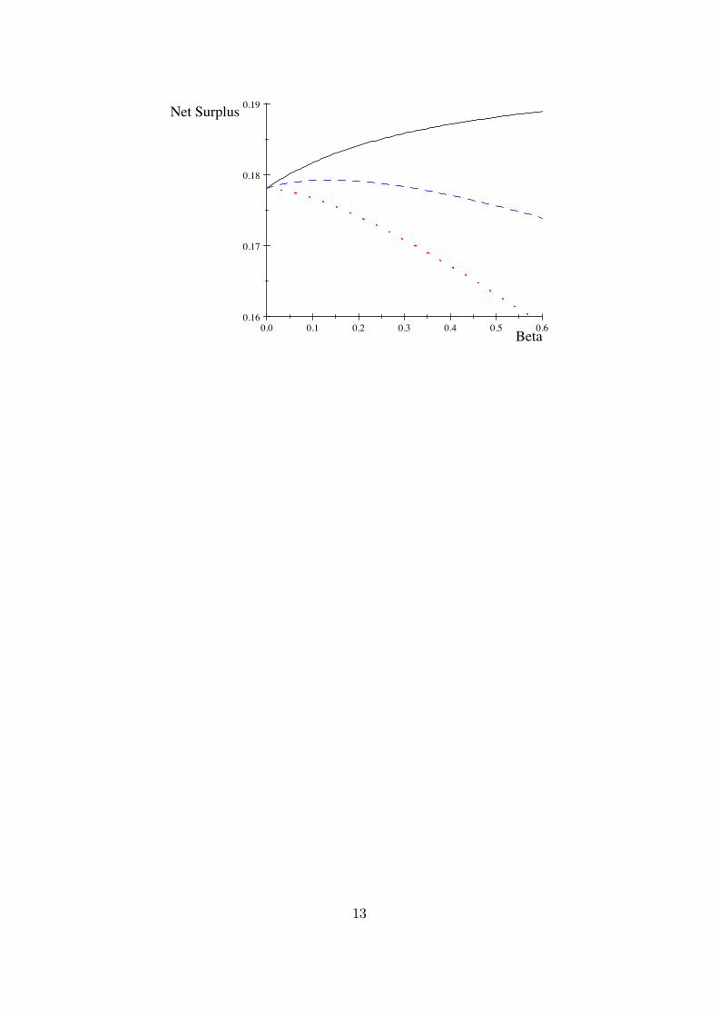
0.0 0.1 0.2 0.3 0.4 0.5 0.60.16

0.17

0.18

0.19

Beta

Net Surplus

13