dynamic coast - national coastal change assessment

Scotland’s centre of expertise for waters

Dynamic Coast - National Coastal Change Assessment: Methodology

Published by CREW – Scotland’s Centre of Expertise for Waters. CREW connects research and

policy, delivering objective and robust research and expert opinion to support the development and

implementation of water policy in Scotland. CREW is a partnership between the James Hutton Institute

and all Scottish Higher Education Institutes supported by MASTS. The Centre is funded by the Scottish

Government.

Please reference this report as follows: Fitton, J.M., Hansom, J.D., and Rennie, A.F. (2017) Dynamic

Coast - National Coastal Change Assessment: Methodology, CRW2014/2.

Dissemination status: Unrestricted

All rights reserved. No part of this publication may be reproduced, modified or stored in a retrieval

system without the prior written permission of CREW management. While every effort is made to ensure

that the information given here is accurate, no legal responsibility is accepted for any errors, omissions

or misleading statements. All statements, views and opinions expressed in this paper are attributable to

the author(s) who contribute to the activities of CREW and do not necessarily represent those of the host

institutions or funders.


National Coastal Change Assessment Steering Committee

Scotland’s National Coastal Change Assessment

1

Methodology Dynamic Coast – Scotland’s National Coastal Change Assessment

Executive Summary

The amount and rate of change on the Scottish Coast has been established by comparing the historic positions of MHWS over time at three time periods, 1890, 1970 and modern.

These rates and positions allow a forecast or forward look to be calculated of the anticipated positions of MHWS in 2050 and 2050+, and of the assets that might be impacted in the future by erosion.

The location of MHWS on the 1890 and 1970 maps are defined by their published and plotted positions by the Ordnance Survey.

The modern position of MHWS depicted on Digital Terrain Models (DTMs) extracted from aerial photography or LiDAR require to be geo-located for altitude and the MHWS line then extracted using a standard methodology.

The method adopted to compute the MHWS height relative to Ordnance Datum (OD) used the harmonic analysis method of the National Oceanography Centre (NOC) POLTIPS software and the MHWS height between these known POLTIPS points was linearly interpolated to derive a height and thus a position.


2

Contents

Executive Summary ................................................................................................................................. 1

1.0 Introduction ................................................................................................................................ 3

2.0 Definitions ................................................................................................................................... 3

2.1 Mean High Water Spring ............................................................................................................... 3

2.2 Normal Tidal Limit ......................................................................................................................... 3

3.0 Whole Coast Assessment Methodology ..................................................................................... 3

4.0 NCCA Coastal Change Methodology ........................................................................................... 4

4.1 Coastal Type .................................................................................................................................. 4

4.2 Plotting the Historic Coastline Position ........................................................................................ 6

4.3 Plotting the Current Coastline Position ...................................................................................... 11

4.4 Historic and Current Coastline Comparison ................................................................................ 16

5.0 Availability of modern terrain height data................................................................................ 17

6.0 Data Structure ........................................................................................................................... 18

7.0 Future Coastline Position Estimates ......................................................................................... 20

7.1 Coastal Erosion ............................................................................................................................ 20

7.2 Accretion ..................................................................................................................................... 21

8.0 Vulnerability Assessment .......................................................................................................... 22

9.0 3D Analysis of Coastal Change .................................................................................................. 22

9.1 Background ................................................................................................................................. 22

9.2 Selection of Test Area ................................................................................................................. 23

9.3 Selection of Datasets .................................................................................................................. 23

9.4 Methodology ............................................................................................................................... 24

9.5 Results & Interpretation ............................................................................................................. 24

9.6 Summary of 3D Analysis.............................................................................................................. 29

References ............................................................................................................................................ 31


3

1.0 Introduction This document describes the methodologies used within the National Coastal Change Assessment (NCCA).

2.0 Definitions In order to assist the understanding of the methodology that follows, the definitions of key terms are defined below.

2.1 Mean High Water Spring

2.1.1 Scotland In Scotland, Ordnance Survey data represents a high and low water mark for the average spring tide.

The line reflecting the alignment of the mean spring high tide is attributed with a Function of ‘Mean High Water Spring Mark’.

The line reflecting the alignment of the average mean spring low tide is attributed with a Function of ‘Mean Low Water Spring Mark’.

If the alignments are coincident then the line is attributed with a function of ‘Mean High Water Spring Mark and Mean Low Water Spring Mark’.

2.1.2 Accuracy requirements The positional accuracy for tide line capture is constrained by the precision and stability of the feature being measured. Tidal marks that lie on unconsolidated material such as mud or sand may be subject to frequent vertical and horizontal movement resulting from erosion or extreme events. Additionally tidal marks on shallow sloping surfaces are prone to significant changes in horizontal position as a result of a small change in tidal height.

Conversely tide lines on steeply sloping surfaces or hard material (natural or manmade) are likely to be more accurate and less prone to horizontal change.

When capturing a tide line by measurement at the correct state of the tide, the actual height of the measured tide must be within 0.3m of the predicted value.

When capturing a tide line by identifying the appropriate contour (through direct capture or interpolation from a Digital Terrain Model) the contour must be measured to an accuracy of 0.3m.

2.2 Normal Tidal Limit A further mark indicated within Geobase-04 data is the Normal Tidal Limit. This is an indication of the point along tidal rivers where mean tides (in England and Wales) or spring tides (in Scotland) affect the level of the water in the river.

3.0 Whole Coast Assessment Methodology To appreciate the distribution and proximity of assets to the shoreline, the asset (or receptor) datasets have been compared against a series of buffers measured from the MHWS: 500m, 200m, 100m, 50m and 10m. Given the complexity of the shoreline a 1:25,000 mapping dataset was used (Ordnance Survey Vector Map District), which maintains much detail whilst not being too complex to process within our Geographic Information System. Attempts were made to buffer the OS MasterMap MHWS line, though this proved too detailed given existing computing power. The asset/receptor dataset used is directly comparable to that used by SEPA within the National Flood


4

Risk Assessment, but has been supplemented with additional road, water network and heritage sites.

The OS Vector Map District polygon was converted into a line dataset, subdivided into smaller sections of coast, buffered and merged to create a single buffered shoreline at 10 m, 50 m, 100 m, 200 m and 500 m. These were then clipped with the original polygon to exclude the foreshore.

Each of the asset datasets were then intersected with the Coastal Type, derived within the NCCA (see section 4.1) to establish if these assets are located on Hard & Mixed, Soft or Artificial Shores. The asset datasets were also considered alongside Fitton’s (2016) measure of inherent erodibility of the coastal zone (Fitton et al 2016, UPSM/CESM+80). Unlike the NCCA Method which uses an adjusted version of Coastal Erosion Susceptibility Model (CESM +40) within the Whole Coast Assessment we’ve used a slightly different section of factors which exclude coastal proximity. The Whole Coast Assessment used the UPSM which incorporates the ground elevation, rock head altitude (i.e. amount of erodible material above) and wave exposure but does not incorporate the presence of coastal defences, nor coastal proximity. As a result it can be used to identify which assets may be susceptible to erosion in the long term, or if defences fail or are not maintained into the future. Once intersected the number, length and area of assets were compiled and reported.

4.0 NCCA Coastal Change Methodology To estimate coastal change on national scales, three discrete methods were used to output various different datasets, which when combined fulfil the requirements of the NCCA. In order to prioritise and analyse the coastal change outputs, the coastal type (either soft, hard and mixed, or artificial coast) was required. Following on from this, the historic high water mark from two time periods; the 1898-1904 coastline and the 1970’s coastline needed to be extracted. Lastly, the modern high water mark needed to be established, preferably using digital terrain models. The methodologies used to complete these tasks are described in turn below.

4.1 Coastal Type The NCCA aims to focus upon those areas where coastal change is most likely, and thus are a priority for management. Hence, there was a requirement to identify those locations that are characterised by soft or dynamic shorelines, so that these key sites can be targeted and prioritised over sites that are rocky, steeper and much less dynamic. To assist with identification of the soft coast the Coastal Erosion Susceptibility Model (CESM) was used. The CESM is a raster based model (50 m cell size) where a number of physical datasets (ground elevation, rockhead elevation, wave exposure, and proximity to the coast) are ranked in order to identify areas with high erosion susceptibility. In this respect the rockhead layer within the CESM was ideally suited to identify areas of land where the rockhead was below MHWS and thus had a sedimentary veneer susceptible to erosion. These areas are identified as soft coast. Aerial photography (dating from the last 6 years) was then used within these areas to fine-tune the process of identification of soft coast in greater detail. This new dataset then supersedes (by some way) the earlier and less accurate classifications undertaken as part of the EUrosion (2004) project. The MHWS was taken from the 2014 (June) update of the OS MasterMap, this being the latest update available on the project start-up. Using the rockhead layers from the CESM, and aerial photography, the soft coast was selected from the MHWS tide line, based on the following criteria:


5

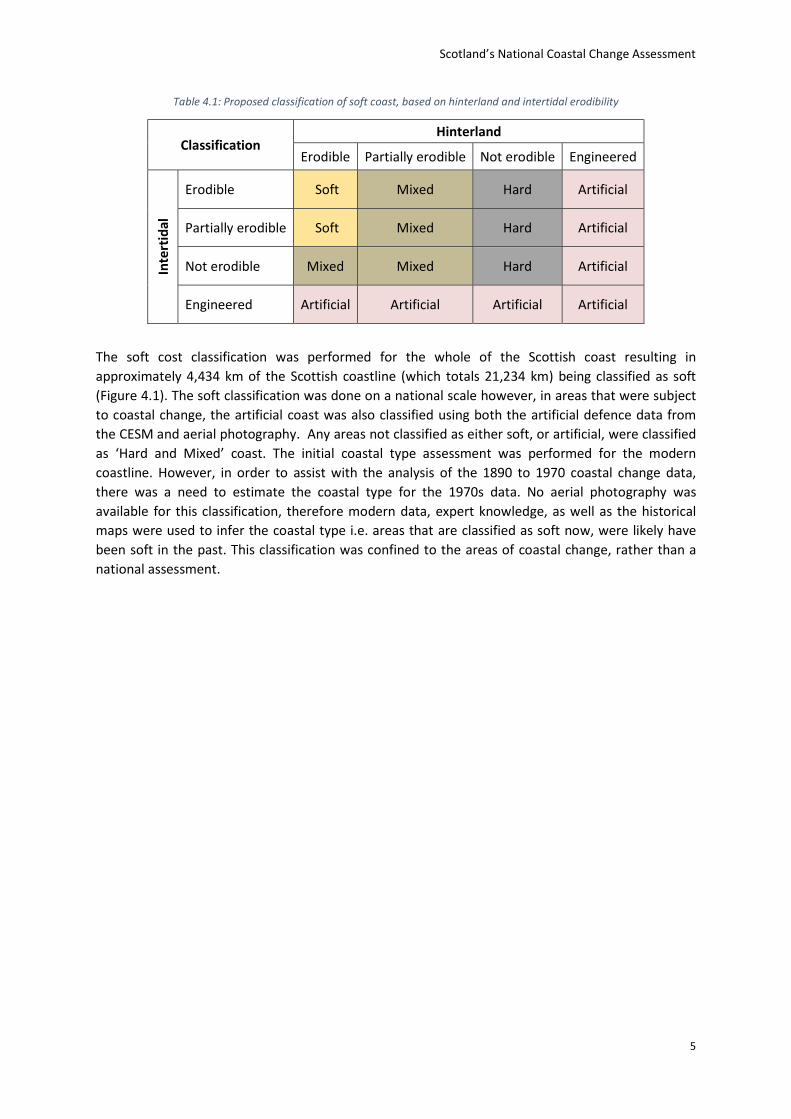
Table 4.1: Proposed classification of soft coast, based on hinterland and intertidal erodibility

Classification Hinterland

Erodible Partially erodible Not erodible Engineered In

tert

idal

Erodible Soft Mixed Hard Artificial

Partially erodible Soft Mixed Hard Artificial

Not erodible Mixed Mixed Hard Artificial

Engineered Artificial Artificial Artificial Artificial

The soft cost classification was performed for the whole of the Scottish coast resulting in approximately 4,434 km of the Scottish coastline (which totals 21,234 km) being classified as soft (Figure 4.1). The soft classification was done on a national scale however, in areas that were subject to coastal change, the artificial coast was also classified using both the artificial defence data from the CESM and aerial photography. Any areas not classified as either soft, or artificial, were classified as ‘Hard and Mixed’ coast. The initial coastal type assessment was performed for the modern coastline. However, in order to assist with the analysis of the 1890 to 1970 coastal change data, there was a need to estimate the coastal type for the 1970s data. No aerial photography was available for this classification, therefore modern data, expert knowledge, as well as the historical maps were used to infer the coastal type i.e. areas that are classified as soft now, were likely have been soft in the past. This classification was confined to the areas of coastal change, rather than a national assessment.


6

Figure 4.1: Coast classified as ‘soft’.

4.2 Plotting the Historic Coastline Position

4.2.1 OS Six-Inch County Edition Second Edition Sheets The Ordnance Survey (OS) Six-Inch County Series Second Edition sheets were published between 1898 and 1904. According to Sutherland (2012) the high water tide line on the Scottish Country Series maps was surveyed by OS surveyor using tide tables to ascertain when high tides that most closely correspond to ‘High Water Mark of Ordinary Spring Tides’ (HWMOST)1 would occur. The surveys were to be made during calm weather and with the high tide line captured by one of two methods:

1 The HWMOST became MHWS in later OS maps, however this is a terminology modification and the definitions remain unchanged. The height of mean high water springs is the average throughout the year of two successive high waters during those periods of 24 hours when the range of the tide is at its greatest. The values of MHWS vary from year to year with a cycle of approximately 18.6 years. (National Tidal and Sea Level Facility, 2017)


7

Objects were placed on the beach at the time of high water. The positions of the objects were surveyed and the surveyed points were joined to form the tide line;

The mark left by high tide was surveyed.

Figure 4.2: Example of an original OS Six-Inch Second Edition sheet.

The original published paper sheets consist of the map detail, along with a substantial border (Figure 4.2). The original paper sheets were digitally scanned by the National Library of Scotland (NLS). NLS cropped the border on the digital version, leaving only the map detail. The resulting four corners of the sheet were then georeferenced (from the County Series Cassini projections to the National Grid). The coordinates for the sheet boundaries were obtained from the Charles Close Society, specifically the Brian Adams/Ed Fielden coordinates (http://www.fieldenmaps.info/cconv/).

Using the georeferencing process above some sheets show a positional error which varies across Scotland. The NLS estimate that parts of the Borders and Central Belt are 5-10 yards (4.5-9 m) from their true position, whereas parts of the Western and Northern Isles may be as much as 30 yards (27m) from their true position. This error has been attributed to four possible sources:

1. The sheet line coordinates obtained are incorrect, or incorrect for certain counties.

2. The conversions between the County Series Cassini projections and the OS National Grid have introduced errors.

3. The conversion between the OS 1858 datum used for the original County Series and more recent OSGB1936 / WGS84 datums have introduced errors.

4. Warping / distortion of the original (paper) OS sheets over time – particularly for A0 sheets.

For use within the NCCA these positional errors needed to be corrected. However, no systematic approach (e.g. adjusting datum conversions) exists that can be used to correct for the errors highlighted above, partly since the error sources may vary between sheets. Therefore, the method used was to manually georectify the NLS positioned sheets (informally known as ‘rubber sheeting’). Modern OS 1:10,000 maps were used to identify features that are congruent in both maps. Where two features exactly matched, a ground control point (GCPs) was established. The GCPs consisted


8

predominantly of the corners of buildings, field boundaries and boundary intersections. However, in some rural coastal areas, due to the lack of identifiable features, this was not possible. In this case stable sections of coastline (such as rocky promontories, headlands or cliffs) that show a clear match were used. Using such coastal features as GCPs was unavoidable and if this approach was not adopted then some rural areas would show considerable error. Once the GCPs were determined the sheet was transformed using the ‘spline’ adjustment to ensure that the transformation passed exactly through the GCPs. Where there was no offset between adjacent sheets, the sheets were joined together prior to georectification to reduce the number of GCPs required.

4.2.2 ‘OS 1970s’ Sheets The NLS have scanned and georeferenced the OS National Grid 1:10,560/1:10,000 sheets for Great Britain with dates closest to 1970. For the purposes of the NCCA this is referred to as the ‘OS 1970s’ dataset. From this OS 1970s dataset, the sheets that intersect the Scottish coast were extracted for use within the NCCA. In these maps the OS terminology of Mean High Water Springs (or MHWS) is used instead of HWMOST, however this is only a terminology modification and the definitions remain unchanged. The MHWS line was plotted around the coast by calculating its elevation by linear interpolation between tidal gauges based at primary and secondary ports (where the elevation of MHWS was directly measured). The interpolated elevations were then used to plot the contour of MHWS at the appropriate elevation (the ground elevations were derived from stereo pairs of analogue aerial photographs which were used to define an elevation model). The derived tidal level and the date of photography defines the date of the resultant MHWS line.

A breakdown of the year surveying ended for each sheet within the OS 1970’s data is shown in Table 4.2, with the spatial distribution shown in Figure 4.3. As these sheets were originally produced using the National Grid projection, no further transformation is needed, and they can be used without further adjustment. The date that surveying ended for each sheet will be used within the coastal change rate analysis to identify the temporal change between coastlines.

Table 4.2: Year surveying ended for the coastal sheets included in the 'OS 1970s' dataset for Scotland

Epoch Number of

Sheets Percentage of

Sheets

1950’s 17 1 %

1960’s 239 15 %

1970’s 954 61 %

1980’s 246 16 %

1990’s 102 7 %


9

Figure 4.3: Spatial distribution of the year surveying ended for the coastal sheets included in the 'OS 1970s' dataset. The sheets for Northern England are represented here for completeness but are not included in the calculations shown Figure 4.2.

4.2.3 Historic Coastline Extraction The high water mark from the adjusted OS Six-Inch County Series Second Edition sheets and the ‘OS 1970’s’ sheets was extracted. For the OS Six-Inch Inch County Series Second Edition, the ‘High Water Mark of Ordinary Spring Tides’ (HWMOST) was mapped, and in the ‘OS 1970’s data the Mean High Water Springs (MHWS) was mapped (note this is just a difference of terminology, the definitions are


10

the same). The high water mark was extracted using a combination of manually and automated extraction. The manual extraction required the use graphics tablet which allows the high water mark to be traced using a stylus (within the NCCA the Wacom Cinitq 24HD graphics tablet was used). The autmoted extraction used the ArcScan toolbar with ArcMap. The digitised high water mark was and linked across sheet boundaries, and then assigned the appropriate metadata e.g. survey dates, sheet number, and length (in metres) etc. For the 1970s data, the coastal type (soft, artificial, hard and mixed) was also included.

Figure 4.4: Coastal change analysis along a narrow estuary in Tiree showing the problem when the Normal Tidal Limit extends far inland. Shades of red indicate erosion, shades of green accretion. Yellow is no change. Bing Maps used for backdrop photography.

Two contexts were identified where extracting the high water mark was deemed to be unnecessary given the objectives of the NCCA. These were:

Where the Normal Tidal Limit (NTL) extends a distance (ca. greater than 200 m) upstream within moderate to narrow inlets, and the channel becomes dominated by fluvial rather than coastal processes (Figure 4.4). Although these channels are technically still coastal, the dynamic and mobile nature of the channels, and their historic and current location on the OS maps is often characterised by advance or retreat. These areas were not analysed so that other areas could be prioritised. Digitisation of the high water mark therefore did not occur more than 300 m upstream of a narrow estuaries/inlet;

There are numerous islands and skerries around the main coastline of Scotland. The high water mark of these islands can be established but only at a considerable cost of time related to extensive digitisation. Since many such islands and skerries are rocky with little change in the position of the coast and with no assets of importance within these islands,

200 m


11

they were removed from the analysis to allow other areas to be prioritised. Where islands are involved then the focus of the NCCA is on ‘inhabited’ islands. A combination of island size, asset data and expert knowledge was used to determine whether to include islands within the analysis.

4.3 Plotting the Current Coastline Position The current position of MHWS on modern OS maps is generated in a similar manner to the methodology used by the OS, outlined in Section 4.2.2. However, instead of using solely aerial photography to derive a ground elevation, LiDAR and aerial photography was used to generate digital elevation models (DEMs). To ascertain the current position of MHWS it was necessary to establish its elevation (relative to Ordnance Datum (OD)) around the Scottish coast taking into account tidal variation and sea level rise. Once established, this elevation was used along with a DEM (derived from LiDAR or aerial photography) to extract the MHWS position. ArcGIS 10.2 was used for the analysis. The methodology used is described below.

4.3.1 MHWS Elevation Within Scotland the OS data represents a high water mark for the average spring tide i.e. MHWS but in order to plot the MHWS line as a contour, the elevation (Z) of MHWS is required. To compute MHWS elevations around the UK coast, the National Oceanography Centre (NOC) developed a software package named POLTIPS. The tidal heights computed within the POLTIPS software uses the harmonic analysis method, developed by the NOC some 75 years ago and now used throughout the world.

Figure 4.5: A brief outline of the data and methodologies used to produce the tidal heights computed within the POLTIPS software package. Adjusted from National Oceanography Centre (2014).

Tidal variations are a result of a number of different phenomena and in order to accurately predict the tides for a location the individual sine waves (harmonic constituents) of these phenomena need to be identified. Harmonic analysis is the process of mathematically identifying the series of sine waves of varying amplitude, phase and speed which best define the period of observations being analysed (National Oceanography Centre, 2014)Up to 240 individual harmonic constituents are used to derive the resultant tide. Once the harmonic constants are established, tidal heights can be


12

accurately predicted for many years forwards or backwards in time. A brief description of the method to produce the tidal heights is shown in Figure 4.5.

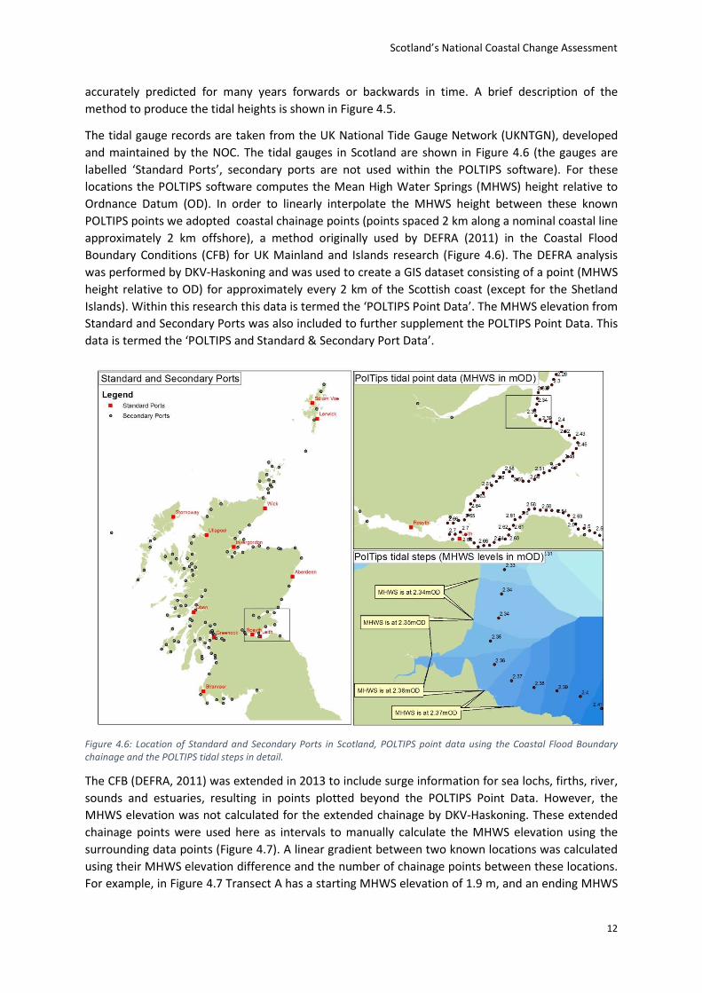
The tidal gauge records are taken from the UK National Tide Gauge Network (UKNTGN), developed and maintained by the NOC. The tidal gauges in Scotland are shown in Figure 4.6 (the gauges are labelled ‘Standard Ports’, secondary ports are not used within the POLTIPS software). For these locations the POLTIPS software computes the Mean High Water Springs (MHWS) height relative to Ordnance Datum (OD). In order to linearly interpolate the MHWS height between these known POLTIPS points we adopted coastal chainage points (points spaced 2 km along a nominal coastal line approximately 2 km offshore), a method originally used by DEFRA (2011) in the Coastal Flood Boundary Conditions (CFB) for UK Mainland and Islands research (Figure 4.6). The DEFRA analysis was performed by DKV-Haskoning and was used to create a GIS dataset consisting of a point (MHWS height relative to OD) for approximately every 2 km of the Scottish coast (except for the Shetland Islands). Within this research this data is termed the ‘POLTIPS Point Data’. The MHWS elevation from Standard and Secondary Ports was also included to further supplement the POLTIPS Point Data. This data is termed the ‘POLTIPS and Standard & Secondary Port Data’.

Figure 4.6: Location of Standard and Secondary Ports in Scotland, POLTIPS point data using the Coastal Flood Boundary chainage and the POLTIPS tidal steps in detail.

The CFB (DEFRA, 2011) was extended in 2013 to include surge information for sea lochs, firths, river, sounds and estuaries, resulting in points plotted beyond the POLTIPS Point Data. However, the MHWS elevation was not calculated for the extended chainage by DKV-Haskoning. These extended chainage points were used here as intervals to manually calculate the MHWS elevation using the surrounding data points (Figure 4.7). A linear gradient between two known locations was calculated using their MHWS elevation difference and the number of chainage points between these locations. For example, in Figure 4.7 Transect A has a starting MHWS elevation of 1.9 m, and an ending MHWS


13

elevation of 2.44 m (taken from the POLTIPS and Standard & Secondary Port data) with eight intervening points along the transect. A linear gradient increment was calculated for the intervening eight chainage points as follows:

𝑀𝐻𝑊𝑆 𝐸𝑙𝑒𝑣𝑎𝑡𝑖𝑜𝑛 𝐷𝑖𝑓𝑓𝑒𝑟𝑒𝑛𝑐𝑒

𝑁𝑢𝑚𝑏𝑒𝑟 𝑜𝑓 𝑇𝑟𝑎𝑛𝑠𝑒𝑐𝑡 𝑃𝑜𝑖𝑛𝑡𝑠 − 1=

(2.44 − 1.9)

(10 − 1)= 0.06 𝑚

and this increment was added to each subsequent point along the transect starting from 1.9 m, until the value of 2.44 was reached.

Figure 4.7: Example of Loch Linnhe (A and B), Loch Leven (C), and Loch Eil (D) showing how the MHWS elevations were calculated for the extension chainage using the POLTIPS and Standard & Secondary Port data. Transects A and B were calculated using a linear gradient, whereas C and D used a constant elevation. See text for further explanation.

A

B

C

D


14

Figure 4.8: The ‘mhws_elev’ raster derived from the MHWS Elevation Point Data and the ’spline with barriers’. Units for elevations are metres above Ordnance Datum (mAOD)

The same method was used for Transect B, using an MHWS elevation change of 0.42 m (2.44-2.02) distributed over nine transect points (0.525 m change between transect points). Transects C and D


15

were calculated differently as there was no upstream/landward data to allow for the calculation of a gradient. Subsequently, the MHWS elevation (either from the POLTIPS and Standard & Secondary Port data, or from an elevation calculated as a gradient) closest to the most downstream/seaward point of the transect was used as a constant along the remaining length of the transect. This process was repeated for all of the extended chainage points, apart from Shetland (the MHWS elevation data and chainage points did not allow for the linear gradient to be calculated), and for some points within the Outer Hebrides (which were deemed redundant due to the close proximity of other extended chainage points). A point dataset including the POLTIPS, Standard and Secondary Ports, and the calculated MHWS elevation chainage was then created. This data is termed the ‘MHWS Elevation Point Data’.

Once the MHWS Elevation Point Data had been established, the position of MHWS relative to the land surface was calculated using a DEM to extract a contour which matches the MHWS elevation. In order for the MHWS elevation data to be useable the point data was then converted into a raster. This is performed using the ‘Spline with Barriers’ tool within ArcGIS (using a smoothing value of 0.5). This tool interpolates a smoothed raster surface between the MHWS Elevation points using a minimum curvature spline technique. Using a polygon which represents the land as a barrier forces the interpolation to be calculated only for the sea surface. The interpolated raster output has a 50 m cell size, and extends 400 m inland so that the raster is compatible with the DTMs for extraction of the MHWS contour. The output is termed the ‘mhws_elev’ raster, which can be seen in Figure 4.8.

Once the elevation of MHWS have been established (the ‘mhws_elev’ raster), the position can be calculated by using the DTM to extract a contour which matches the MHWS elevation. The methodology used is briefly described below:

The DTM is clipped to a buffer of 400 m either side of OS MasterMap MHWS;

To smooth the data, the ‘Focal Statistics’ tool was run on the DTM with a 7 x 7 m cell

neighbourhood;

To further smooth the DTM the ‘Fill’ tool was also run to remove any isolated cells that are

completely surrounded by cells with higher elevations;

The ‘mhws_elev’ raster was then clipped, resampled and snapped to match the extent, cell

size and position of the DTM raster;

Where the ‘mhws_elev’ raster and the DTM overlap, the raster calculator was then used to

extract the cells (and assigned a value of 1) from the DTM that were equal to, or less than,

the height of MHWS i.e. the value of the ‘mhws_elev’ raster. The formula used within the

raster calculator was: Con("DTM" <="mhws_elev", 1 )

This raster was converted to a polygon, then to a polyline. The polyline line was then

cleaned automatically to remove any lines resulting from the boundaries of the dataset

rather than actual data;

The polyline was then smoothed using the ‘Smooth Line’ tool with the PAEK algorithm and a

tolerance of 4 m. The ‘Smooth Line’ tool was rerun again on the smoothed line (using the

same settings as previous) to further smooth the line.


16

4.4 Historic and Current Coastline Comparison In order to establish the amount and rate of coastal change over time, the two historic and the current MHWS positions were compared. For regional to national scale assessments of coastal change, a grid cell based approach will used. The method used is as follows:

A point at 10 m intervals was places on the historic and current coastlines (Figure 4.9a). This

will have the effect of splitting the polyline into coastal change units (CCUs) of 10 m in length

(5 m either side of the plotted point);

Using the ‘Near’ tool, the distance between each of the 1890s to 1970s points, and 1970s to

modern points was established (Figure 4.9b);

To establish which sections of coastline were eroding or accreting, a polygon representing

the land for each coastline (termed the ‘inland polygon’) was also generated for the 1890s

and 1970s time period. Where a CCU point from the 1970s, was located inside the 1890s

inland polygon boundary, or a modern CCU point was located inside the 1970s inland

polygon boundary, the near distance was multiplied by -1, causing the rate to become a

negative. Where the CCU points lay outside of the inland polygon boundary, the distance

was multiplied by 1. Hence, a negative distance designates erosion, where as a positive rate

is a sign of accretion. This value was termed DIST_V (V signifying that the distance had a

vector);

The point data was then joined back to the CCU line, hence the output at this stage is a

polyline split at 10 m intervals, with a vectored distance representing change;

The time difference between the two coastlines (using the survey end date) was calculated

and a rate of change was established (distance divided by time) for each CCU;

The change rate extrapolated over 10 and 25 years was then calculated (change rate x 10 or

25);


17

Figure 4.9: Hypothetical scenario demonstrating the coastal change methodology a) points are plotted at a 10 m interval along each of the coastlines b) the distance between the coastline points is calculated. Note only erosion is shown in this figure: areas of accretion will also be assessed using the same methodology.

5.0 Availability of modern terrain height data Deriving a modern MHWS line not only requires an up to date tidal level, but also requires a representative topographic dataset, ideally in the form of 3-dimensional digital terrain models (DTMs). In dynamic areas it is imperative to have as recent a topographic surface as possible to ensure the resultant line work remains an accurate representation.

SNH collated a Pan-Government Remote Sensing Data Index (RSDI) to include all the pan-Scotland surveys it was aware of and had access to. This data set is shown in Figure 5.1 below.


18

Figure 5.1: Mapped representation of The Pan-Government Remote Sensing Data Index (draft)

The above RSDI data set allows the reappraisal of large sections of the mainland east coast, including the main firths and more spatially limited areas elsewhere. Whilst SNH and Historic Scotland datasets have been included, the largest surveys were undertaken to support SEPA’s flood risk management work. Most of the DTMs have been derived from Phase 1 and Phase 2 LiDAR, with additional DTMs created from other LiDAR and aerial photographic surveys.

6.0 Data Structure The methodologies above resulted in a total of five datasets being created; historic coastlines for the 1890s and 1970s, a modern coastline position, and coastal change data for 1890s to 1970s and 1970s to modern. As well as the spatial data, the outputs have a further attribute data attached. The


19

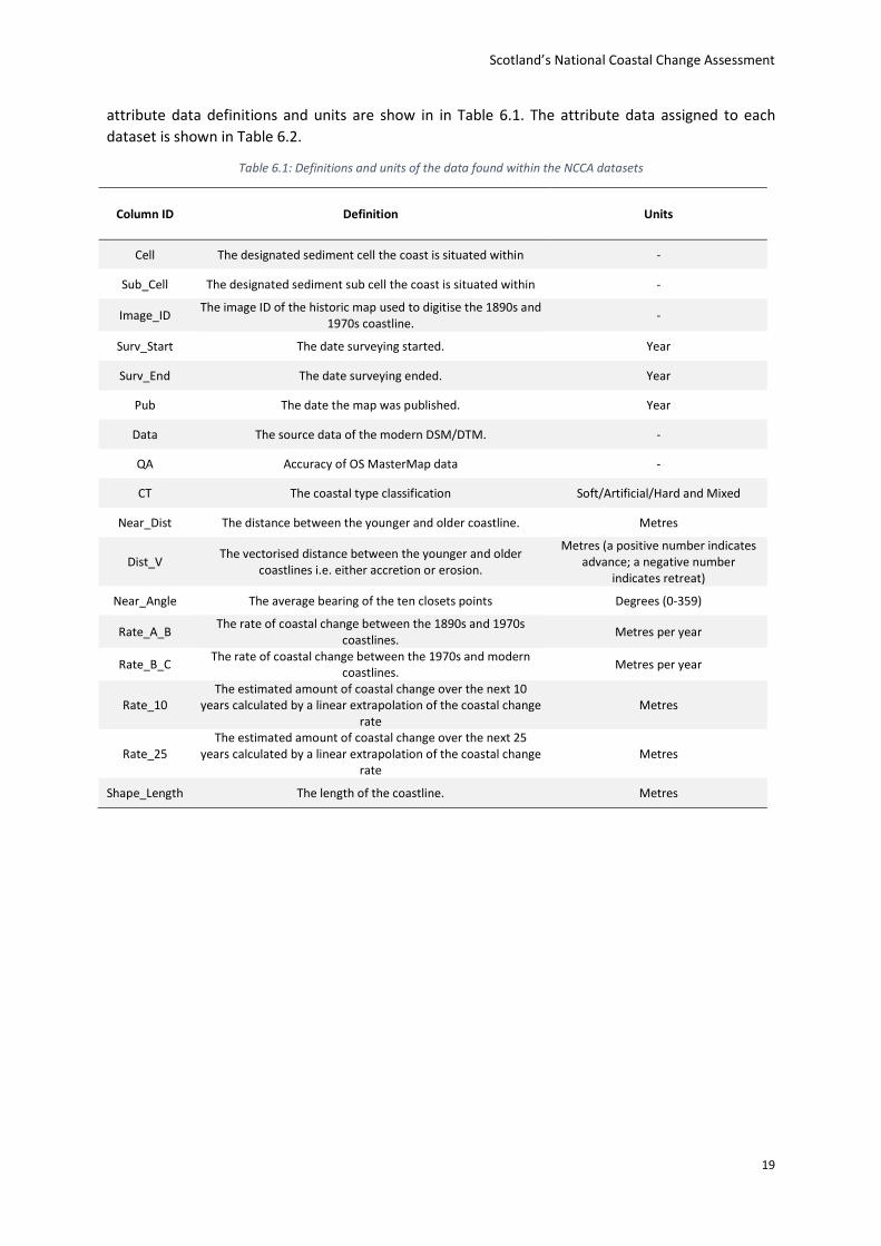
attribute data definitions and units are show in in Table 6.1. The attribute data assigned to each dataset is shown in Table 6.2.

Table 6.1: Definitions and units of the data found within the NCCA datasets

Column ID Definition Units

Cell The designated sediment cell the coast is situated within -

Sub_Cell The designated sediment sub cell the coast is situated within -

Image_ID The image ID of the historic map used to digitise the 1890s and

1970s coastline. -

Surv_Start The date surveying started. Year

Surv_End The date surveying ended. Year

Pub The date the map was published. Year

Data The source data of the modern DSM/DTM. -

QA Accuracy of OS MasterMap data -

CT The coastal type classification Soft/Artificial/Hard and Mixed

Near_Dist The distance between the younger and older coastline. Metres

Dist_V The vectorised distance between the younger and older

coastlines i.e. either accretion or erosion.

Metres (a positive number indicates advance; a negative number

indicates retreat)

Near_Angle The average bearing of the ten closets points Degrees (0-359)

Rate_A_B The rate of coastal change between the 1890s and 1970s

coastlines. Metres per year

Rate_B_C The rate of coastal change between the 1970s and modern coastlines.

Metres per year

Rate_10 The estimated amount of coastal change over the next 10

years calculated by a linear extrapolation of the coastal change rate

Metres

Rate_25 The estimated amount of coastal change over the next 25

years calculated by a linear extrapolation of the coastal change rate

Metres

Shape_Length The length of the coastline. Metres


20

Table 6.2: Data included within each of the data sets.

Column ID Data

1890 (A suffix)

1970 (B suffix)

Modern (C suffix)

1890 to 1970 Change 1970 to Modern Change

Cell

Sub_Cell

Image_ID

Surv_End

Pub

Data

QA

CT

Near_Dist

Near_Angle

Dist_V

Rate_A_B

Rate_B_C

Rate_10

Rate_25

Shape_Length

7.0 Future Coastline Position Estimates Once the coastal change rates have been established, the amount of change expected by 2050 can be estimated. The methods used for coastal erosion and accretion are different and are explained in turn. It is important to note that no consideration for the impacts of climate change e.g. sea level rise, change in storm frequency, are incorporated into these future projections. The future projections are an extrapolation of past rates to two future time steps.

7.1 Coastal Erosion To forecast the coastline position on eroding coastlines, the yearly coastal change rate (calculated in Section 4.4 is multiplied by the appropriate number of years (e.g. a coastal change rate of 1.5 m per year, equals 75 m of change over 50 years) the CCU is then projected the appropriate distance (Figure 7.1a) in land. The projected area is then converted to a polygon and smoothed to create an erosion polygon (Figure 7.1b). The Coastal Erosion Susceptibility Model (CESM) (Fitton et al., 2016) was used to more accurately determine the hinterland extent of possible erosion. The CESM is a raster based model (50 m cell size) where a number of physical datasets (ground elevation, rockhead elevation, wave exposure, and proximity to the coast) are ranked in order to identify areas with high erosion susceptibility. The CESM is modified to remove the influence of the proximity to the coast parameter and included in the analysis by erasing from the future erosion polygon areas that are deemed to have a CESM score of equal to or less than 40 i.e. areas that do not have the inherent physical characteristics to allow erosion (Figure 7.1c and Figure 7.1d).


21

Figure 7.1: Hypothetical scenario demonstrating the future coastline methodology a) the polyline CCUs generated via the 10 m point intervals created in Section 4.4 are projected to 2050, and 2050+ using the calculated coastal change rates b) the projected CCU is converted to a smoothed polygon c) the CESM is used to only allow erosion in areas that are physically susceptible to erosion d) the CESM shows that the right hand side of the coastline has low susceptibility and is therefore removed from the predicted future erosion area.

7.1.1 Coastal Erosion Buffers Once the coastal erosion area had been produced a series of buffers were created around this area. The first, labelled the erosion influence zone, is a 10 m buffer around the main erosion area. This buffer was created as some assets can be negatively impacted by coastal erosion indirectly as these assets are now situated closer to MHWS. For example, the school at Balivanich, Benbecula has now been abandoned, as boulders are often over washed into the school grounds, causing significant damage. A further buffer 50 m beyond the erosion influence zone was also generated to ensure that any vulnerability assessment is able to inform analysis about the assets that are situated close to areas of coastal erosion that may be indirectly affected by the coastal erosion/loss of other assets.

7.1.2 Future Scenario: 2050+ Due to the effects of climate change there is potential for future erosion rates to increase. To estimate the possible impacts of this coastal erosion zones and buffers were generated that represent the amount of erosion expected by 2100 at current rates. However, these data can be interpreted as the consequence of an approximate doubling of current coastal erosion rates, and therefore provide information for future planning.

7.2 Accretion For the majority of areas, where coastal accretion has been identified between the 1970s and the modern MHWS position, a 5 m buffer along the coast is generated. This is to indicate that accretion will possibly continue at this location. However, in locations where knowledge from other data sources exist e.g. historic data, academic literature, previous field surveys, expert knowledge etc. it is possible to estimate the future position of MHWS more accurately. In these locations a manual edit is performed to delineate the possible future position of MHWS. In general, these manual edits have been performed in locations where accretion is parallel to the shore e.g. Culbin Sands, and along spits, e.g. North Tentsmuir.


22

Such an approach is necessary as whilst accretion is simply the net accumulation of sediment and erosion is the net removal of sediment, projecting each of these changes forward works better for erosion, but creates unlikely situations with accretion. Given the influence of wave and tidal processes, accumulated sediment is readily spread along a section of coast. An influx of sediment may also lead to the building up of coastal landforms, which is increasingly likely on a rising sea level. For this reason it is more realistic to highlight the accretionary shores with a 5 m buffer, unless lateral coastal development is anticipated (i.e. on spits, like Culbin’s Flying Bar).

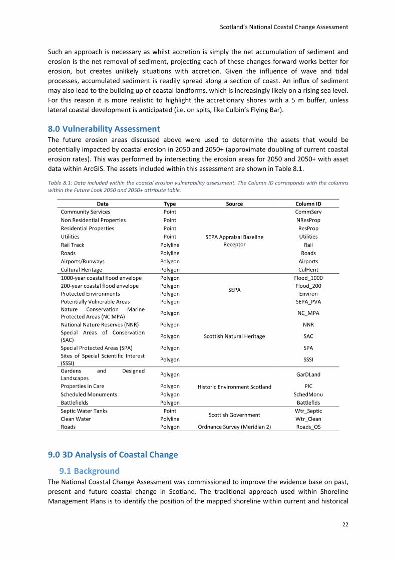
8.0 Vulnerability Assessment The future erosion areas discussed above were used to determine the assets that would be potentially impacted by coastal erosion in 2050 and 2050+ (approximate doubling of current coastal erosion rates). This was performed by intersecting the erosion areas for 2050 and 2050+ with asset data within ArcGIS. The assets included within this assessment are shown in Table 8.1.

Table 8.1: Data included within the coastal erosion vulnerability assessment. The Column ID corresponds with the columns within the Future Look 2050 and 2050+ attribute table.

Data Type Source Column ID Community Services Point

SEPA Appraisal Baseline Receptor

CommServ Non Residential Properties Point NResProp Residential Properties Point ResProp Utilities Point Utilities Rail Track Polyline Rail Roads Polyline Roads Airports/Runways Polygon Airports Cultural Heritage Polygon CulHerit 1000-year coastal flood envelope Polygon

SEPA

Flood_1000 200-year coastal flood envelope Polygon Flood_200 Protected Environments Polygon Environ Potentially Vulnerable Areas Polygon SEPA_PVA Nature Conservation Marine Protected Areas (NC MPA) Polygon

Scottish Natural Heritage

NC_MPA

National Nature Reserves (NNR) Polygon NNR Special Areas of Conservation (SAC)

Polygon SAC

Special Protected Areas (SPA) Polygon SPA Sites of Special Scientific Interest (SSSI)

Polygon SSSI

Gardens and Designed Landscapes

Polygon

Historic Environment Scotland

GarDLand

Properties in Care Polygon PIC Scheduled Monuments Polygon SchedMonu Battlefields Polygon Battleflds Septic Water Tanks Point

Scottish Government Wtr_Septic

Clean Water Polyline Wtr_Clean Roads Polygon Ordnance Survey (Meridian 2) Roads_OS

9.0 3D Analysis of Coastal Change

9.1 Background The National Coastal Change Assessment was commissioned to improve the evidence base on past, present and future coastal change in Scotland. The traditional approach used within Shoreline Management Plans is to identify the position of the mapped shoreline within current and historical


23

maps; in this case this is the position of Mean High Water Springs and its predecessor High Water Mark of Ordinary Spring Tides. The changing position through time of these lines allows areas of erosion and accretion to be identified; however this approach only identifies changes along that specific contour and says nothing of the changes elsewhere across the shore face. The use of MHWS as a proxy for the surrounding landforms has been sufficient for over a hundred years (Parliamentary commission into coastal erosion, 1915) however technological improvements now allow surfaces to be more readily surveyed, compared and disseminated.

Below summarises a trail of these techniques to explore the benefits of the 3D approach.

9.2 Selection of Test Area To adequately test the approaches a section of coast needed to be selected with at least two sets of high quality height data. This would allow comparisons between the surfaces and the single contour of MHWS.

Early liaison with the Ordnance Survey (OS) suggested that Digital Surface Models (DSMs) could be created for Tiree using 2011 photography. This complemented the LiDAR derived DSM collected by SNH in 2006 and allow relatively recent change to be identified and compared against ground observation of recent coastal erosion. The added benefit of this approach is that the ground observations identified that the erosion was ongoing and the creation of a dataset after 2006 would prove valuable.

The OS processed 2011 imagery, however once inspected by the NCCA team there were numerous artefacts and datum issues. A request was made to the OS to correct these datasets, but in the intervening time our attention turned to other suitable sites.

The Golspie links (Sutherland) had multiple datasets given partnership working following recent storms. Whilst smaller than Tiree, this site had experience of recent storms, erosion, over topping and floods damaging assets within the coastal zone.

9.3 Selection of Datasets Whilst the northern section of the Golspie Links was covered by the Scottish Government LiDAR survey (Phase 1) in 2011, the area to the south was not collected. Due to SNH’s involvement within research and partnership work, they had commissioned aerial surveys in 2013 and 2015. The University of Glasgow had also undertaken ground GPS surveys and Terrestrial Laser Scan Surveys which were also made available.

Table 9.1: Dates and summary of impacts of storms on Golspie Links

Date of storm Summary of Impact within Links

14th Dec 2012 Extensive erosion, over-wash, flooding and damage to Golf Course, Caravan Park & Kart Track. The NNR was inundated.

Feb 2014 Localised erosion, over-wash, flooding and damage to Golf Course, Caravan Park, & Kart Track. The NNR was inundated.

6th & 7th Oct 2014 Localised erosion, over-wash, flooding and damage to Golf Course, Caravan Park, & Kart Track. The NNR was inundated.


24

9.4 Methodology

9.4.1 2D Analysis Whilst full methods are available within the Methodology Report a summary is presented here. The historical and current maps were loaded into the GIS software and checked to ensure their spatial positioning was correct. Mean High Water Springs / High Water Mark of Ordinary Spring Tides were then digitised to create a line depicting the position of each. The spatial changes between these were then investigated using semi-automatic processes to quantify the change through time. The aerial survey from 2013 was also analysed to extract the ‘modern’ MHWS line.

9.4.2 3D Analysis The Digital Surface Models (DSMs) were loaded within the GIS software and checked for errors or anomalies. The Feb 2013 DSM was created by digital photogrammetry, whereby overlapping vertical aerial images are analysed to produce a 3D surface extending from the outskirts of Golspie (in the north) to the mouth of Loch Fleet (in the south). Within this section the area of greatest interest was resurveyed in October 2014. During the intervening 14 months there had been two storms.

The two surfaces were aligned on to the same grid and resampled to ensure that accurate comparisons could be made. The area of overlap within these surveys was then compared for height changes, by subtracting the newer altitudes from the older surface. This produces a ‘change surface’ with gains in altitude shown as positive values and surface lowering as negative values. The patterns of change were then inspected and identifiable areas of change were then partitioned to allow the changes in separate parts of the beach to be quantified.

The smaller 2014 surface was then embedded within the larger 2013 surface to allow more realistic visualisations to be undertaken. Whilst the analysis thus far has been done using ArcGIS software the preparation of web-based virtual landscapes were done using QGIS.

9.5 Results & Interpretation

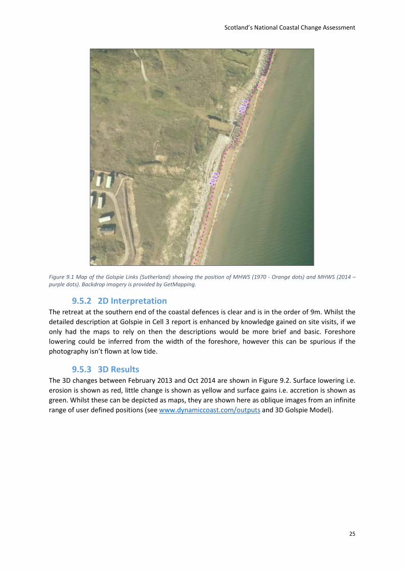
9.5.1 2D Results The 2D changes between MHWS position in 1970 (yellow dotted line) are compared with the MHWS position in 2014 (purple dotted line) in Figure 9.1. These lines alongside the 1890 shoreline are available via the web-maps (www.dynamiccoast.com).


25

Figure 9.1 Map of the Golspie Links (Sutherland) showing the position of MHWS (1970 - Orange dots) and MHWS (2014 – purple dots). Backdrop imagery is provided by GetMapping.

9.5.2 2D Interpretation The retreat at the southern end of the coastal defences is clear and is in the order of 9m. Whilst the detailed description at Golspie in Cell 3 report is enhanced by knowledge gained on site visits, if we only had the maps to rely on then the descriptions would be more brief and basic. Foreshore lowering could be inferred from the width of the foreshore, however this can be spurious if the photography isn’t flown at low tide.

9.5.3 3D Results The 3D changes between February 2013 and Oct 2014 are shown in Figure 9.2. Surface lowering i.e. erosion is shown as red, little change is shown as yellow and surface gains i.e. accretion is shown as green. Whilst these can be depicted as maps, they are shown here as oblique images from an infinite range of user defined positions (see www.dynamiccoast.com/outputs and 3D Golspie Model).


26

Figure 9.2 three-dimensional model of coastal changes at Golspie Links (looking south). Erosion / surface lowering shown in reds, little change in Yellows and Gains / Accretion / Repairs shown in green. See text for further description. Backdrop imagery provided by CASL © SNH.

9.5.1 3D Interpretation Figure 9.2 identifies considerable mid-beach lowering in reds downdrift of the defences (Label A), along with losses within the crest, the central one (Label B) provided the flooding corridor into the dune interior. Interesting the greatest losses were further along (Label C) which wasn’t breached in the 2014 storm. The mid-beach and dune crest losses are quantifiable (Figure 9.3 and Figure 9.4) and enable management responses, in this case the identification of the necessary volume of gravel to feed the beach to return it to a 2013 pre-storm profile.

It should be noted that given the accuracy of the 3D datasets, they offer a degree of precision beyond that of the 2D analysis. For example, in Figure 9.1 there has been 9 m retreat between 1970 and 2013 which is under the significance threshold for the NCCA (i.e. less than 10 m). However, the 3D surfaces depict far more detailed and informative changes from a single storm, thereby allowing more detailed and considered appreciation of erosion but also flood risk and resilience.

Given recent improvements in computing technology the 3D surfaces are more readily viewed via web browsers. This revolutionises the user’s opportunity to inspect and learn about the changes and the data. By comparing multiple datasets within a virtual reality webpage, the user is about to see the pre and post-storm landscapes and quantify the changes and flood levels in real time (Figure 9.5). To see this model and one for the Bay of Skaill see www.dynamiccoast.com/outputs.

Another benefit of 3D analysis is greater clarity of more subtle changes further up the beach than MHWS. This is of particular importance for Historic Environment Scotland and recent observed risks within their Properties of Care. The topographic changes at Skara Brae between 2014 and 2016 are shown in Figure 9.6, with pockets of erosion along the crest-line of the beach. This location is more

A

B

C


27

likely to contain archaeological interests than the mid to upper beach (MHWS) which is likely to experience seasonal changes alongside repeated erosion and depositional cycles during and following storms. A similar process of beach crest erosion is known to be occurring at Fort George (Moray Firth) despite MHWS remaining stable within our analysis.

Figure 9.3 Sediment Budget for Golspie Links, showing partitioned volumetric changes (m3) based on 2013 to 2014 coastal changes.


28

Figure 9.4: Partitions used to analysis the volumetric changes shown within Figure 9.3


29

Figure 9.5: 3D viewer displaying topographic change between 2013 & 14 and an arbitrary flood level.

Figure 9.6: 3D view of erosion along the beach crest (reds) between 2014 and 2016. © HES.

9.6 Summary of 3D Analysis 1) Two-dimensional (2D) approaches use the changing position of a single contour as a proxy

for changes across the lower, mid and upper foreshore. This significant simplification does not occur within three-dimensional (3D) analyses, where actual changes are compared, rather than inferred from a proxy measure.


30

2) 3D analyses can offer a far higher level of understanding than 2D approaches, as they confer greater detail on actual changes rather than infer possible changes.

3) 3D analyses also have considerable advantages in the interpretation of changes, where more nuanced changes are apparent. This is particularly the case with non-specialists.

4) 3D analysis requires at least two accurate surveys to be readily available, which may not be the case in many areas. In these instances aerial photography can be used to construct supplementary surveys.

5) Whilst the NCCA has relied on 2D to MHWS, the availability of 3D data is far more informative where erosion influences flood risk and resilience, but also where the beach face behaves in more complex ways (i.e. Skara Brae (Orkney), Fort George (Moray Firth)).


31

References Fitton, J.M., Hansom, J.D. & Rennie, A.F. (2016) A national coastal erosion susceptibility model for

Scotland. Ocean & Coastal Management, 132, pp.80–89. Available from: <http://dx.doi.org/10.1016/j.ocecoaman.2016.08.018>.

Hansom, Dunlop and Roberts (2015) Golspie Links Coastal Erosion Assessment 2013-2014 (ver 2015-02-05)

Hansom JD and Fitton JM (2013) Golspie dunes coastal erosion options appraisal. SNH Commissioned Report CR635

National Oceanography Centre (2014) TASK - Tidal Analysis Software Kit User Guide.

National Tidal and Sea Level Facility (2017) Definitions of tidal levels and other parameters [Internet]. Available from: <http://www.ntslf.org/tgi/definitions> [Accessed 26 June 2015].

Sutherland, J. (2012) Error analysis of Ordnance Survey map tidelines, UK. Proceedings of the ICE - Maritime Engineering, 165, pp.189–197.

CREW Facilitation Team

James Hutton Institute

Craigiebuckler

Aberdeen AB15 8QH

Scotland UK

Tel: +44 (0)1224 395 395

Email: [email protected]

www.crew.ac.uk


CREW is a Scottish Government funded partnership between

the James Hutton Institute and Scottish Universities.

dynamic coast - national coastal change assessment

Documents