tsunami coastal hazard along the us east coast from
TRANSCRIPT

Tsunami Coastal Hazard Along the Us East CoastFrom Coseismic Sources in the açoresConvergence Zone and the Caribbean Arc AreasStephan Toni Grilli ( [email protected] )
University of Rhode Island https://orcid.org/0000-0001-8615-4585Maryam Mohammadpour
University of Rhode IslandLauren Schambach
University of Rhode IslandAnnette Grilli
University of Rhode Island
Research Article
Keywords: Tsunami hazard assessment, Tsunami propagation, earthquakes, Boussinesq wave models
Posted Date: April 13th, 2021
DOI: https://doi.org/10.21203/rs.3.rs-404526/v1
License: This work is licensed under a Creative Commons Attribution 4.0 International License. Read Full License
Version of Record: A version of this preprint was published at Natural Hazards on November 15th, 2021.See the published version at https://doi.org/10.1007/s11069-021-05103-y.

Noname manuscript No.(will be inserted by the editor)
Tsunami coastal hazard along the US East Coast from1
coseismic sources in the Acores Convergence Zone and the2
Caribbean Arc areas3
Stephan T. Grilli · Maryam Mohammadpour ·4
Lauren Schambach · Annette R. Grilli5
6
April 2, 20217
Abstract We model the coastal hazard caused by tsunamis along the US East Coast (USEC)8
for far-field coseismic sources originated in the Acores Convergence Zone (ACZ), and the9
Puerto Rico Trench (PRT)/Caribbean Arc area. In earlier work, similar modeling was per-10
formed for probable maximum tsunamis (PMTs) resulting from coseismic, submarine mass11
failure and volcanic collapse sources in the Atlantic Ocean basin, based on which tsunami12
inundation maps were developed in high hazard areas of the USEC. Here, in preparation13
for a future Probabilistic Tsunami Hazard Analysis (PTHA), we model a collection of 1814
coseismic sources with magnitude ranging from M8 to M9 and return periods estimated in15
the 100-2,000 year range. Most sources are hypothetical, based on the seismo-tectonic data16
known for the considered areas. However, the largest sources from the ACZ, which includes17
the region of the Madeira Tore Rise, are parameterized as repeats of the 1755 M8.6-9 (Lis-18
bon) earthquake and tsunami using information from many studies published on this event,19
which is believed to have occurred east of the MTR. Many other large events have been doc-20
S.T. Grilli
Department of Ocean Engineering, University of Rhode Island, Narragansett, RI, USA
E-mail: [email protected]
M. Mohammadpour
Department of Ocean Engineering, University of Rhode Island, Narragansett, RI, USA
E-mail: [email protected]
L. Schambach
Department of Ocean Engineering, University of Rhode Island, Narragansett, RI, USA
E-mail: [email protected]
A.R. Grilli
Department of Ocean Engineering, University of Rhode Island, Narragansett, RI, USA
E-mail: annette [email protected]

2 Grilli et al.
umented to have occurred in this area in the past 2,000 years. There have also been many21
large historical coseismic tsunamis in and near the Puerto Rico Trench (PRT) area, triggered22
by earthquakes with the largest in the past 225 years having an estimated M8.1 magnitude.23
In this area, coseismic sources are parameterized based on information from a 2019 USGS24
Powell Center expert, attended by the first author, and a collection of SIFT subfaults for the25
area (Gica et al., 2008).26
For each source, regional tsunami hazard assessment is performed along the USEC at a27
coarse 450 m resolution by simulating tsunami propagation to the USEC with FUNWAVE-28
TVD (a nonlinear and dispersive (2D) Boussinesq model), in nested grids. Tsunami coastal29
hazard is represented by four metrics, computed along the 5 m isobath, which quantify inun-30
dation, navigation, structural, and evacuation hazards: (1) maximum surface elevation; (2)31
maximum current velocity; (3) maximum momentum force; and (4) tsunami arrival time.32
Overall, the first three factors are larger, the larger the source magnitude, and their along-33
shore variation shows similar patterns of higher and lower values, due to bathymetric control34
from the wide USEC shelf, causing similar wave refraction patterns of focusing/defocusing35
for each tsunami. The fourth factor differs mostly between sources from each area (ACZ36
and PRT), but less so among sources from the same area; its inverse is used as a measure37
of increased hazard associated with short warning/evacuation times. Finally, a new tsunami38
intensity index (TII) is computed, that attaches a score to each metric within 5 hazard inten-39
sity classes selected for each factor, reflecting low, medium low, medium, high and highest40
hazard, and is computed as a weighted average of these scores (weights can be selected to41
reinforce the effect of certain metrics). For each source, the TII provides an overall tsunami42
hazard intensity along the USEC coast that allows both a comparison among sources and43
a quantification of tsunami hazard as a function of the source return period. At the most44
impacted areas of the USEC (0.1 percentile), we find that tsunami hazard in the 100-50045
year return period range is commensurate with that posed by category 3-5 tropical cyclones,46
taking into account the larger current velocities and forces caused by tsunami waves.47
Based on results of this work, high-resolution inundation PTHA maps will be developed48
in the future, similar to the PMT maps, in areas identified to have higher tsunami hazard,49
using more levels of nested grids, to achieve a 10-30 m resolution along the coast.50
Keywords Tsunami hazard assessment · Tsunami propagation · earthquakes · Boussinesq51
wave models52

US East Coast tsunami impact 3
1 Introduction53
Since 2010, under the auspice of the US National Tsunami Hazard Mitigation Program54
(NTHMP; http://nthmp.tsunami.gov/index.html), the authors and colleagues55
have performed tsunami modeling work to develop high-resolution tsunami inundation maps56
for the US east coast (USEC), starting with the most critical or vulnerable areas, but with the57
goal to eventually to cover the entire coast. These so-called first generation maps were con-58
structed as envelopes of maximum inundation caused by the most extreme near- and far-field59
tsunami sources in the Atlantic Ocean basin, a.k.a., Probable Maximum Tsunamis (PMTs),60
parameterized based on historical or hypothetical events [48]. In this first generation work,61
no return periods were considered for each source and probabilistic tsunami hazard analyses62
(PTHA) were left out for future work. Extreme tsunamigenic sources causing PMTs that63
can impact the USEC have been identified and modeled in past work [2,3,34,4,32,55,17,64
36,8,13,23,1,19,20,24,25,21,27,57,54,49,37,45]. These sources were divided into three65
groups: 1) coseismic, 2) submarine mass failure (SMF), and 3) volcanic flank collapse. An66
overview of the global coastal hazard resulting from these sources, at the coarse regional67
scale, can be found in Schambach et al. [48].68
Fig. 1 Footprint and ETOPO1 bathymetry/topography (color scale in meter shows <> 0) of FUNWAVE’s
1 arc-min resolution grids in North Atlantic Ocean basin (Local/Large G0), with footprints of 3 regional 450
m nested shore-parallel Cartesian grids (G1, G2, G3; Table 4). Location are marked for the two areas of
historical/hypothetical tsunami coseismic sources (red oval) considered, near the Acores Convergence Zone
(ACZ), including Lisbon 1755 (LSB), and near and around the Puerto Rico Trench (PRT). The Madeira Torre
Rise (MTR) is the shallower ridge located on the north of the ACZ circled area and the Horseshoe Plain is
to the East of the ACZ and MTR. Yellow/red symbols within the regional grids mark locations of numerical
wave gauge stations where time series of surface elevation are calculated in simulations for validating the
one-way grid coupling (Table 2).

4 Grilli et al.
The present work is part of the initial preparatory steps necessary to perform a complete69
PTHA for the USEC and create the next generation of probabilistic NTHMP inundation70
maps. PTHA, instead of only considering PMTs, requires combining simulation results for71
a collection of tsunami sources of different magnitudes and, hence, return periods for each72
type of sources. Here, we only consider far-field coseismic sources in the North Atlantic73
Ocean Basin (NAOB), which are the only seismic sources that can be sufficiently tsunami-74
genic to cause a significant tsunami hazard along the USEC, where near-field seismicity is75
quite moderate [55,57]. Additionally, coseismic sources, as a group, are believed to have76
lower return periods than the SMF and volcanic collapse sources in the NAOB [55,57].77
Hence, in its lower impact range, this work also provides a first comprehensive assess-78
ment of regional scale tsunami hazard for the entire USEC, for a range of return periods79
commensurate with those considered in risk analyses for coastal and ocean structures and80
infrastructures, for other natural hazard events such as tropical cyclones (e.g., 100 to 50081
years).82
We consider and model coseismic tsunamis generated by a collection of seismic sources83
located near and around (Fig. 1): (i) the Acores Convergence Zone (ACZ; Fig. 1 and see Fig.84
18 in [57]), including the estimated location of the 1755 Lisbon (LSM) earthquake source,85
and (ii) the Puerto Rico Trench (PRT) and Caribbean arc area [33,56,28,21]. Several large86
tsunamigenic earthquakes have occurred in these areas. In the ACZ/LSB area, which is lo-87
cated along the western segment of the Eurasia-Nubia Plate Boundary, between the Azores88
archipelago and the Strait of Gibraltar [7], some of these historical earthquakes have caused89
large transoceanic tsunamis, but the Lisbon 1755 earthquake, of estimated magnitude M8.6-90
9 [41,8], triggered the largest known historical tsunami. With 5-15 m high waves impacting91
the coast, this event caused extensive destruction and tens of thousands of fatalities, in the92
near-field in Lisbon and its area (in combination with seismicity and fires), while also reach-93
ing the coasts of Morocco, England, Newfoundland, Brazil, and the Antilles. In particular,94
after transoceanic propagation, the LSB 1755 tsunami still caused a few meters of inunda-95
tion in the eastern Lesser Antilles [2,3,62,4,8,5,57,7]. Large coseismic tsunamis have also96
occurred in the PRT and Caribbean arc area [33,55,23,40], which a highly seismic area97
running parallel to the north shore of Hispaniola, Puerto Rico, and the north-eastern lesser98
Antilles [11,62,55,56,23,28,57] (see Fig. 1 for the observed distribution of earthquakes,99
in magnitude and depth). The PRT is the only subduction zone in the NAOB, in which the100
North America Plate subducts under the Caribbean Plate with a nearly E-W relative plate101
motion (i.e., largely left lateral strike slip; see large black arrows in Fig. 1) and only a small102
component of perpendicular convergence (3-6 mm/yr) [11,9]. Nevertheless, in: (i) 1842, a103
M8 earthquake in the western segments of the Septentrional fault (SF), which runs nearshore104
parallel to the north shore of Hispaniola, triggered a large tsunami that impacted in Haiti [12,105

US East Coast tsunami impact 5
16,21]; (ii) 1787, a M8.1 in the PRT triggered a moderate tsunami; and (iii) 1918, a M7.3106
earthquakes in the Mona Passage, 15 km off the northwest coast or Puerto Rico, generated a107
tsunami that caused 116 fatalities and up to 6 m runup [40,35]. Since the Indian Ocean M9.2108
earthquake and tsunami [22,30], we know that highly oblique subduction zones can generate109
devastating tsunamis if the earthquake rupture has a large thrust component. Although this is110
still controversial, some work has shown that a tsunamigenic M8.7-9 earthquake in the PRT111
would cause a devastating tsunami in the near-field and a significantly damaging event in112
the far-field, particularly along the upper USEC [32,23]. A recent meeting of experts at the113
USGS Powell Center (May 2019) reached the conclusion that such large PRT events were114
possible, however, the upper bound magnitude would likely require that fault segments in115
part of Hispaniola on the West and the Caribbean arc (up to Guadeloupe) on the East be also116
involved (this is further detailed later).117
In this work, we parameterize and simulate tsunamis generated by coseismic sources118
sited in the two selected areas, ranging from magnitude M8 to M9. For the ACZ/LSB area,119
we will define sources sited at two different locations and having 2 different orientations120
(strike) of 15 and 345 deg. from North, besides different magnitude (M8-M9) and corre-121
sponding fault plate areas; this yields ten (10) different coseismic tsunami sources, four of122
these being the M9 PMT sources already considered in earlier NTHMP inundation mapping123
work [19,48]. Due the large uncertainty of sources in this area, each source is only repre-124
sented by a single fault plane. As in earlier work considering PMTs [19], the two selected125
orientations are aimed at maximizing tsunami impact on the upper and lower USEC, respec-126
tively. Since the LSB/ACZ sources are quite distant from the USEC, tsunami propagation127
and refraction over the entire ocean width make details of the sources relatively less impor-128
tant [54], hence our earlier work that also considered additional orientations for the sources129
showed that these two selected strike angles were sufficient to reflect tsunami hazard along130
the USEC. We shall see that a repeat of the LSB M9 1755 event, particularly if it occurred131
in the ACZ, West of the Madeira Torre Rise (Fig. 1), a submarine ridge that somewhat di-132
verted the transoceanic propagation of the historical event towards the USEC, would have133
the potential for causing high tsunami hazard along the entire USEC. In the PRT area, we134
only model hypothetical events, following the recommendations on fault plane segmenta-135
tion made during the 2019 Powell Center meeting of expert, and consider eight (8) M8-M9136
sources that combine 10 to 26 SIFT (Short-term Inundation Forecast for Tsunamis) sub-137
faults [17], with for comparison one of these being the M9 PMT source already considered138
in earlier NTHMP inundation mapping work [23,20,48].139
Tsunami simulations are performed for the 18 selected coseismic sources using the fully140
nonlinear and dispersive Boussinesq model FUNWAVE-TVD [61,50,31], by one-way cou-141
pling in a series of nested spherical or Cartesian coordinate grids. FUNWAVE has been142

6 Grilli et al.
validated for a collection of tsunami benchmarks [53,29], and used in the simulation of143
many historical [60,22,30,51,24,31,52,21,26,46,47] and hypothetical [23,1,25,54,49,27,144
45] tsunami case studies. As we only aim at assessing the global coastal tsunami hazard145
caused by the selected sources along the USEC, we only use two levels of nested grids146
(Fig. 1): (i) two large scale spherical grids over the North Atlantic Ocean (or half of it),147
with a 1 arc-min resolution, and (ii) 3 smaller regional shore-parallel Cartesian grids over-148
lapping along the USEC with a 450 m resolution. For each source, because of the coarse149
resolution of the coastal grids, we will assess tsunami hazard using several metrics, com-150
puted at a short distance from shore, along the 5 m isobath and will leave inundation and151
runup simulations out for future work using higher-resolution grids. Based on similar re-152
sults obtained for a collection of PMTs selected in the North Atlantic Ocean [48], as part153
of NTHMP work, high-resolution inundation maps were computed for the envelope of all154
the PMT results in USEC areas that were deemed at higher hazard or being critical (see155
project webpage: https://www1.udel.edu/kirby/nthmp.html). To do so, ad-156
ditional levels of nested grids were used to achieve a 10-30 m resolution at the coast (see,157
for instance, [25]). Note, however, although complex coastal morphologies and highly devel-158
oped areas will be under-resolved at a 450 m resolution, from Florida to Massachusetts, the159
USEC is essentially made of a series of sandy barrier beach and barrier-island whose coastal160
bathymetry is quite simple, and hence coarse grid results should be accurate up to a short161
distance from shore and reflection off the coast also be sufficiently accurately represented162
in the model. In their simulations of the impact of the 2004 Indian Ocean tsunami along the163
coasts of Thailand, using FUNWAVE in a 450 m resolution nested grid, Ioualalen et al. [30]164
showed a good agreement between the predicted and observed runups at 58 locations.165
Based on results of the present work, obtained for eighteen coseismic sources of various166
magnitude (and hence return period), and similar results for other types of sources to be167
obtained in future work (i.e., for submarine landslides, volcanic flank collapse, and meteo-168
tsunamis), PTHA analyses will be conducted and probabilistic inundation maps, similar169
to the current first generation NTHMP maps based on PMTs, will be developed in future170
work in areas identified to have higher tsunami hazard. To more easily identify these areas,171
the coastal tsunami hazard simulated for each source considered here will be quantified172
by computing 4 hazard metrics along the 5 m isobath: (1) maximum surface elevation; (2)173
maximum current velocity; (3) maximum momentum force; and (4) tsunami arrival time.174
Overall, the first three factors are larger, the larger the source magnitude, and the fourth175
factor is expected to differ mostly between sources from each area (ACZ and PRT), but less176
among sources from the same area.177
Finally, a tsunami hazard intensity index (TII) will be computed for each source, and178
overall, that attaches a score to selected classes of hazard metrics (here 5 classes for each179

US East Coast tsunami impact 7
metric), and provides an overall tsunami hazard intensity (or score) at a large number of180
save points along the 5 m isobath.Similar indices have been proposed in earlier work and181
shown to be usefulness in coastal tsunami hazard assessment, to discriminate between low,182
medium and high hazard coastal areas [42,10].183
In the following, we first detail recent studies of seismic sources in the NOAB and our184
source selection in the two selected areas (ACZ and PRT). We then present the modeling185
methodology and results in terms of the various tsunami hazard metrics computed along the186
USEC and, based on these, we compute and discuss the TII values for each source.187
Fig. 2 Likeliest segmentation in 5 segments of the PRT/Caribbean arc, from west of Hispaniola to Guade-
loupe in the eastern part, established at the May 2019 workshop of experts at the USGS Powell Center (see
Fig. 1 for location). Insert shows footprints of SIFT subfaults [17] in the considered area (see Table 2 for
parameter values). Large black arrows show the nearly E-W relative plate motion of the North America Plate
subducting under the Caribbean Plate.

8 Grilli et al.
2 Recent studies and selection of coseismic sources in the ACZ and PRT areas188
2.1 ACZ/LSB area189
By analyzing the historical sources with information about the occurrence of earthquakes190
and tsunamis in the region of Cape Saint Vincent-Gulf of Cadiz, Udias [59] reviewed large191
tsunamigenic earthquakes that occurred SW of Iberia before the 1755 Lisbon earthquake.192
Separating events that occurred before and after 500 A.D, the author concluded that the193
1755 earthquake and tsunami was not an isolated event in SW Iberia and other similarly194
large events have occurred before the great Lisbon event (e.g., in 241/216 B.C., 881, 1356195
and 1531), which is merely the most resent observed event in this category in the ACZ area196
(Fig. 1). Hence, there is a high likelihood for similarly large events to occur in the future in197
the ACZ/LSB area.198
The exact location and parameters of the 1755 Lisbon earthquake, however, are still199
unknown and subject to debate. Various studies have placed its magnitude in the M8.6 to 9200
range and its most likely location in the Horseshoe Fault to the East of the ACZ and Madeira201
Torre Rise (MTR; Fig. 1) [41,8]. MTR is an underwater ridge that likely caused westward202
propagating tsunami waves to be somewhat diverted from aiming at the USEC and, hence,203
offered some level of protection to the coast. Specifically, Baptista et al. [2,3] performed204
backward ray tracing and located the 1755 Lisbon source in the area between the Gorringe205
Bank and the southwestern end of the Portuguese coast. Based on field surveys and tsunami206
observations, Baptista et al. [4] later proposed a composite source in the Marques de Pombal207
and Guadalquivir faults for the event. Barkan et al. [8] identified three potential coseismic208
tsunami sources for the historical Lisbon event located along three respective major faults,209
including: (i) the Gorringe Bank Fault (GBF); (ii) The Marques de Pombal Fault (MPF); (iii)210
The Gulf of Cadiz Fault (GCF). Based on a set of 16 potential tsunami source simulations211
performed around the areas of these three major faults, Barkan et al. inferred that the most212
likely source of the 1755 earthquake would have been located in the Horseshoe Plain thrust213
fault area (NW/SE strike). However, this fault may just be a paleo plate boundary [7]. Omira214
et al. [44] showed that a source in the Gorringe Bank would have radiated most of its energy215
towards the NE and Morocco, with a minor impact along the Gulf of Cadiz, and proposed216
two more potential locations for the source of the 1755 event, the: (iv) Horseshoe Fault and217
(v) Portimao Bank. They simulated tsunamis from the 5 potential areas and concluded that218
the most likely location was in Horseshoe Fault.219
There have been a few recent tsunamigenic events in the ACZ area, which, although220
they did not generate large tsunamis, confirmed that large future earthquakes could poten-221
tially occur on both sides of the ASZ/MTR area. Hence, in comprehensive tsunami hazard222

US East Coast tsunami impact 9
assessment studies, both of these locations must be considered for siting such future events.223
Specifically, in 1941 a M8.3 strike-slip earthquake occurred in the Gloria fault, northwest224
of the ACZ. A small tsunami was registered at the tide stations of Cascais, Lagos, Portu-225
gal, Morocco, Madeira, Azores (and in the UK), with a maximum observed height of 0.45226
m (peak to peak) at Casablanca in Morocco. In 1969, a M7.9 earthquake occurred in the227
Horseshoe Plain, directly east of the ACZ, which created a small tsunami with a maximum228
height of 0.06 m observed on the Portuguese coast in Lagos. And, in 1975, a M7.9 earth-229
quake occurred south of the Gloria Fault, within the ACZ and southeast of the MTR [6,7]230
(Fig. 1), which generated a tsunami recorded at a set of coastal tide gauges, with a measured231
amplitude of up to 0.3 m in Lagos.232
As part of earlier NTHMP work, Grilli and Grilli [19] designed extreme M9 PMTs orig-233
inated in the ACZ area, as repeats of the Lisbon 1755 event, based on the conclusions of234
Barkan et al.’s [8] study. To cover the range of uncertainty on source location and parame-235
ters, they modeled twelve sources of M9 magnitude sited at various locations in the ACZ,236
with parameters selected based on earlier published work. The strike angle, in particular,237
which strongly affects the tsunami directionality, was varied to cause maximum impact on238
various sections of the USEC. Among those sources, as expected, they found that maximum239
impact on the USEC, with a 1-2 m flow depth at the coast, was created by sources sited240
in the MTR, which is the westernmost potential site for the historical earthquake; arrival241
time on the USEC was between 8 and 12 h, depending on the location. However, should a242
large coseismic source occur west of the MTR, it would cause an even larger impact on the243
USEC. Hence for extreme tsunami hazard assessment, such source locations should also be244
considered for future events.245
Accordingly, in our recent work modeling coastal hazard caused by PMTs along the
USEC as part of NTHMP [48], we considered four (4) so-called Lisbon (LSB) M9 PMTs,
sited at locations both west of the MTR (M9.0-MTR1 and M9.0-MTR2) and east of the
MTR (M9.0-HSP1 and M9.0-HSP2) in the Horseshoe Plain, and with strike angles of 15 or
345 deg. In combination, these sources should maximize the tsunami impact from extreme
PMTs originating in this area along the entire USEC. In the absence of more detailed data,
each source was made of a single fault plane, with parameters based on Barkan et al. [8]
and Grilli and Grilli [19] listed in Table 1. Here, in addition to these extreme sources, to
prepare for future PTHA work along the USEC, we design and parameterize 6 additional
tsunamigenic coseismic sources with 3 smaller magnitudes, M8, 8.3, and 8.7, and for each
the 2 strike angles, whose parameters are also listed in Table 1. All 10 sources are assumed
to be similarly shallow to maximize tsunami generation, with a depth below seafloor d = 5
km at their highest point, and sited at the same location west of the MTR to maximize their
impact on the USEC, except for M9-HSP1 and M9-HSP2, which are sited in the horseshoe

10 Grilli et al.
plain at the likeliest location for the 1755 event. While the M9 sources have a fault plane of
length L = 317 km by width W = 126 km [8], the smaller magnitude sources have reduced
dimensions derived based on the various references listed before. For each coseismic source,
magnitudes M and fault slip S are related by the formulas,
Mo = µLWS (1)
where Mo is the moment magnitude, µ = 40 GPa the material constant (i.e., Coulomb/shear
modulus), and the magnitude is defined as,
M =2
3logMo − 6 (2)
For each source, using the fault plane parameters and location listed in Table 1, Okada’s246
method [43] will be used to compute the initial surface elevation used to initialize the247
tsunami propagation model (see details later).248
Although historical data is limited to accurately attach a return period to each of these249
selected ACZ/LSB events, the average recurrence of large LSB 1755 type events appears to250
be on the order of 500 years [59] (4-5 medium-large events in 2,000 years). Hence, based251
on the corresponding slip and fault area, one could infer that M8, M8.3, and M8.7 events252
would have a return periods of 70, 140, and 250 years with a large uncertainty. These return253
periods are listed in Table 1 for information, as probabilistic considerations will be addressed254
in future PTHA work.255
2.2 PRT and Caribbean Arc area256
While there have been many studies regarding the seismo-tectonic context and past near-257
field tsunamis that have affected the PRT and Caribbean arc area [11,33,62,55,28,57,40]258
(see Fig. 1), until the 2019 Powell Center meeting of experts, no comprehensive study had259
considered the largest tsunamigenic coseismic sources that could affect the USEC, except260
perhaps work performed for the US nuclear regulatory commission [55,56].261
Hence, when tsunami hazard assessment studies were initialed for the USEC, in the262
absence of specific guidance, Knight [32] first proposed a M9.1 PRT source as an extreme263
PMT, which encompassed the 600 km long deepest part of the PRT that runs parallels to the264
Puerto Rico North shore; this source was parameterized by a single fault plane. Using this265
and another similar source with a smaller M8.7 magnitude, Grilli et al. [23] modeled both266
the near-field tsunami impact on Puerto Rico and the far-field impact on the USEC. Based267
on earlier work [15,40,62], they assumed a predominantly (lateral) strike-slip motion of the268
Caribbean plate at 20 mm per year with respect to the North American Plate, in the ENE269
direction, at a 10-20 degree angle with respect to the PRT axis. Analyzing the historical270

US East Coast tsunami impact 11
Source Lat. N. Lon. E. Strike Length Width Slip M ∼ Tr
(ACZ) (deg.) (deg.) θ (deg.) L (km) W (km) S (m) (year)
M8.0-MTR1 36.748 -15.929 15 150 60 2.87 8.0 70
M8.0-MTR2 36.748 -15.929 345 150 60 2.87 8.0 70
M8.3-MTR1 36.748 -15.929 15 175 70 5.95 8.3 140
M8.3-MTR2 36.748 -15.929 345 175 70 5.95 8.3 140
M8.7-MTR1 36.748 -15.929 15 200 80 18.14 8.7 250
M8.7-MTR2 36.748 -15.929 345 200 80 18.14 8.7 250
M9.0-MTR1 36.748 -15.929 15 317 126 20 9.0 500
M9.0-MTR2 36.748 -15.929 345 317 126 20 9.0 500
M9.0-HSP1 36.042 -10.753 15 317 126 20 9.0 500
M9.0-HSP2 36.042 -10.753 345 317 126 20 9.0 500
Table 1 Parameters of coseismic sources modeled as a single fault plane in the ASZ area (Fig. 1), to be used
in Okada’s method [43] to define a tsunami source. All sources are shallow, with a depth d = 5 km at the
mid-fault highest point, and all fault planes are dipping at δ = 40 deg., with the rake being γ = 90 deg.
Estimates of return period Tr for each events are provided for information only and have a large uncertainty.
The M9 sources are Lisbon 1755 proxy sources based on Barkan et al. [8] and Grilli and Grilli [19], while
the M8, 8.3 and 8,7 are smaller magnitude sources modeled to prepare for future PTHA along the USEC.
Except for M9-HSP1 and M9-HSP2, which are sited in the horseshoe plain at the likeliest location for the
1755 event, all sources are centered at the same location west of the MTR (Fig. 1), to maximize impact on
the USEC. Magnitudes and slip are based on a Coulomb modulus µ = 40 GPa. Fig. 4 shows the initial
elevation computed for the 4 largest sources; other sources have similar patterns of elevations and depression,
but smaller amplitude initial surface elevations.
earthquakes and the tsunamigenic events among those, they noted that 12 earthquakes of271
at least a M7 magnitude had occurred in and near the PRT area in the past 500 years [14].272
Among those, two had a M8.1 magnitude, and three generated a tsunami with a 5-7 m on273
Puerto Rico. Combining these observations with the plate convergence rates, they estimated274
that a M7.5-8.1 event in the PRT would have an 80 year return period, a M8.7 event at least275
a 200 year return period, and a M9 event at least a 600 year return period. In view of more276
recent work on the segmentation and fault locking in the area (see below), it is likely that277
these return periods were under-estimated.278
Simulating Knight’s extreme M9 event, Grilli et al. [23] showed that the generated279
tsunami could cause up to 2-3 m runup along the USEC and arrival times would be be-280
tween 2.5 and 6 h, depending on the location. In our initial NTHMP work, in light of new281
data provided on subfault parameters in the PRT/Caribbean arc area as part of NOAA’s SIFT282
dataset [17], Grilli et al. [20] designed and modeled a different M9 PMT source, which ap-283
proximately covered the same area of the PRT as Knight’s [32] source, i.e., 600 km long284
by 150 km wide, but was parameterized as 6 by 2 (i.e., 12) individual SIFT subfaults, each285
100 long by 50 km wide (in the oblique fault plane), which better represented the convex286

12 Grilli et al.
geometry of the PRT. Although this was an extreme scenario, particularly for Puerto Rico,287
their work on the 2004 Indian Ocean M9.2 earthquake [22,30] and devastating tsunami had288
convinced these authors, as others [55,56], that a large megathrust event could occur in the289
PRT because of the similarity between the geometry (both trenches are arched) and plate290
dynamics of the Puerto Rico and Sumatra-Andaman trenches. This was also supported by291
their work on the Tohoku 2011 M9 earthquake and tsunami, that occurred in the similar size292
Japan trench [24,52]. Most recently, simulations of tsunami hazard caused by PMTs on the293
USEC were performed at higher resolution using as one of the sources that of Grilli et al.294
[20], which confirmed the range of runup and arrival time predicted earlier [48].295
In the present work, we needed to design and model a collection of hypothetical, but re-296
alistic, coseismic tsunami sources of various magnitude (and return periods) in the complex297
PRT/Caribbean arc area, that would significantly impact the USEC. As indicated before, a298
meeting of experts was organized in May 2019 at the USGS Powell Center, attended by the299
lead author, whose agenda was devoted in large part to establishing a so-called logic tree300
for coseismic sources in the PRT and Caribbean arc area that could cause tsunamis affect-301
ing the USEC. Such a tree visualizes the various sources and their parameter range, while302
attaching a probability to each branch off the tree. The workshop approach was based on the303
Delphi method, which is a process used to arrive at a group opinion by surveying the experts304
attending the venue. Through several rounds of questionnaires, the responses provided by305
the experts on various source parameters were transformed into tables of probabilities for306
classes of parameter values.307
The consensus of the experts at the meeting was that a first step was, by considering308
existing seismo-tectonic knowledge in the area, to establish a segmentation of the entire309
Caribbean arc into realistic segments, most likely to fail either separately or together in clus-310
ters, and to estimate their parameters. Sources of various magnitude could then be designed311
by combining those segments. Additionally, in the PRT and on both sides of it, there was312
large uncertainty on the level of locking and the magnitude of the fault-normal convergence313
rate that would most contribute to causing large tsunamigenic earthquakes [9], whose range314
needed to be estimated. Figure 2 shows the likeliest segmentation established during the315
meeting, which is composed of 5 segments, of the faults encompassing subduction zones in316
the Hispaniola trench on the west (Segment #1), the PRT in the middle (Segments #2,3), and317
in the northern Lesser Antilles arc (Segments #4,5). Each of these segments approximately318
overlaps with subfaults defined in the SIFT dataset [17] (see insert in Fig. 2). For each SIFT319
subfault, of dimension L = 100 by W = 50 km in the trench-parallel and trench-normal320
directions, respectively, the dataset provides the strike and dip angles, with the rake angle321
assumed as γ = 90 deg. in all cases (to maximize the seafloor deformation), and the lat-lon322
coordinates of the fault centroid and depth d of the fault highest point. Table 2 provides323

US East Coast tsunami impact 13
Segment SIFT Lon. E. Lat. N. Depth Strike Dip
# subfault (deg.) (deg.) d (km) θ (deg.) δ (deg.)
1 atsza57 -72.3535 19.4838 22.10 94.20 20.00
1 atszb57 -72.3206 19.9047 5.00 94.20 20.00
1 atsza56 -71.5368 19.3853 22.10 102.64 20.00
1 atszb56 -71.4386 19.7971 5.00 102.64 20.00
1 atsza55 -70.7045 19.1376 22.10 108.19 20.00
1 atszb55 -70.5647 19.5386 5.00 108.19 20.00
1 atsza54 -69.6740 18.8841 22.10 101.54 20.00
1 atszb54 -69.5846 19.2976 5.00 101.54 20.00
2 atsza53 -68.4547 18.7853 22.10 83.64 20.00
2 atszb53 -68.5042 19.2048 5.00 83.64 20.00
2 atsza52 -67.5412 18.8738 22.10 85.87 20.00
2 atszb52 -67.5734 19.2948 5.00 85.87 20.00
2 atsza51 -66.5742 18.9484 22.10 84.98 20.00
2 atszb51 -66.6133 19.3688 5.00 84.98 20.00
2 atsza50 -65.6921 18.9848 22.10 89.59 20.00
2 atszb50 -65.6953 19.4069 5.00 89.59 20.00
3 atsza49 -64.8153 18.9650 22.10 94.34 20.00
3 atszb49 -64.7814 19.3859 5.00 94.34 20.00
3 atsza48 -63.8800 18.8870 22.10 95.37 20.00
3 atszb48 -63.8382 19.3072 5.00 95.37 20.00
4 atsza47 -63.1649 18.7844 22.10 110.46 20.00
4 atszb47 -63.0087 19.1798 5.00 110.46 20.00
4 atsza46 -62.4217 18.4149 17.94 117.86 15.00
4 atszb46 -62.2075 18.7985 5.00 117.86 15.00
4 atsza45 -61.5491 18.0566 17.94 112.84 15.00
4 atszb45 -61.3716 18.4564 5.00 112.84 15.00
5 atsza44 -61.1559 17.8560 17.94 141.07 15.00
5 atszb44 -60.8008 18.1286 5.00 141.07 15.00
5 atsza43 -60.5996 17.0903 17.94 138.71 15.00
5 atszb43 -60.2580 17.3766 5.00 138.71 15.00
5 atsza42 -59.9029 16.4535 17.94 136.99 15.00
5 atszb42 -59.5716 16.7494 5.00 136.99 15.00
Table 2 SIFT subfault and their parameters from Gica et al. [17], for each segment selected for defining
coseismic tsunami sources in the PRT/Caribbean arc area (Figs. 1 and 1) using the Okada [43] method. In
addition, each subfault has a (horizontal) length L = 100 km, width W = 50 km, and rake γ = 90 deg.
The material constant (shear modulus) used is µ = 40 GPa, as recommended in [17].
these parameters for all the SIFT subfaults overlapping with Segments #1 to 5 from Fig. 2,324
with the subfault locations defined in the figure inset.325
The second step considered by the experts was defining the likeliest grouping of indi-326
vidual segments that would fail together in a single event, thus creating sources of larger327

14 Grilli et al.
magnitude, as well as the associated magnitude for each such event and their likelihood328
(i.e., probability). Although the final proceedings of the workshop are still pending, based329
on draft material from the workshop, Table 2.2 lists 7 new sources in the PRT/Caribbean330
arc area, with magnitudes M8.3, M8.7, and M9.0, that regroup 2 to 4 segments from Fig. 2;331
an additional eighth source M9.0-PRT3 is the extreme PMT source used in earlier work to332
date [20,48]. Based on the SIFT subfault dimensions and their number used for each source333
listed in Table 3, an associated average slip S was computed for using Eqs. 1 and 2, assum-334
ing µ = 40 GPa as in the SIFT study. For each source, using the fault plane parameters and335
location listed in Table 3, Okada’s method [43] will be used to compute the initial surface336
elevation used to initialize the tsunami propagation model (see details later).337
If the maximum convergence rate of ∼20 mm/y (i.e., 1 m of slip in 50 years) in the area338
contributed to the listed slip values, the return period for each source would be ∼75, 185,339
and 355 years, respectively. However, the relative subduction between the Caribbean and340
North-American plates is highly oblique (10-20 deg.) on the western side of the considered341
area and less so in the lesser Antilles (Fig. 2). Accumulated fault slip must be multiplied by342
the sine of the convergence angle; hence, assuming an average of 20 deg. for the entire area343
yields a factor of one-third or so and approximate return periods on the order of 250, 550,344
and 1,000 years for each source magnitude, respectively, which is consistent with estimates345
made during the Powell workshop; applying the same considerations to the M9.0-PRT3346
source, we find an approximate return period of years of 2,000 years (i.e., about 3 times347
the earlier estimate that did not consider the oblique subduction [23]). The estimated return348
periods are listed for each source in Table 2.2, however, detailed probabilistic considerations349
will be left out for future PTHA work.350
3 Methodology351
3.1 Tsunami propagation model352
For each of the selected coseismic sources, tsunami propagation to the USEC is modeled us-353
ing the nonlinear and dispersive two-dimensional (2D) Boussinesq long wave model (BM)354
FUNWAVE [61], in a series of nested grids of increasing resolution, by a one-way coupling355
method. We use FUNWAVE-TVD V.3, the newer implementation of FUNWAVE, which is356
fully nonlinear in Cartesian grids [50] and weakly nonlinear in spherical grids [31]. The357
model was efficiently parallelized for use on a shared memory cluster, which allows us-358
ing large grids. FUNWAVE and then FUNWAVE-TVD are open source codes that have359
been widely used to simulate tsunami case studies [22,30,51,23,1,52,24,31,54,25,21,27,360
26,46,47]. As discussed in the introduction, since 2010 as part of the NTHMP work (see,361

US East Coast tsunami impact 15
Source Segments Nb. Slip M ∼ Tr
(PRT) number SIFT S (m) (year)
M8.3-PRT1 #2 - 3 12 1.3 8.3 250
M8.3-PRT2 #3 - 4 10 1.6 8.3 250
M8.3-PRT3 #4 - 5 12 1.3 8.3 250
M8.7-PRT1 #2 - 4 18 3.5 8.7 550
M8.7-PRT2 #3 - 5 16 3.9 8.7 550
M9.0-PRT1 #1 - 4 26 6.8 9.0 1,000
M9.0-PRT2 #2 - 5 24 7.4 9.0 1,000
M9.0-PRT3 #2 - 3 12 14.8 9.0 2,000
Table 3 Definition in terms of segmentation established at the USGS 2019 Powell Center workshop, of
coseismic sources modeled as multiple SIFT subfault planes in the PRT/Caribbean arc area (Fig. 1), to be
used in Okada’s method [43] to define a tsunami source (Fig. 1). Magnitude and slip (based on a Coulomb
modulus µ = 40 GPa) are given in the table and other parameters of SIFT sources used in each segment are
given in Table 2. Estimates of return period Tr for each events are provided for information only and have a
large uncertainty. The collection of sources is modeled to prepare for future PTHA along the USEC. Fig. 5
shows the initial surface elevations computed for these sources. Note that source M9.0-PRT3 is the extreme
PMT source used in earlier work [23,20,48].
http://chinacat.coastal.udel.edu/nthmp.html; e.g., [1,19,20,25,27,54,45]), the authors have362
used FUNWAVE and related methodology to simulate PMTs and compute tsunami inun-363
dation maps along the USEC. The same model and approach were also used to perform364
several other tsunami hazard assessment studies of coastal nuclear power plants in the U.S.365
Both spherical and Cartesian versions of FUNWAVE-TVD were validated through bench-366
marking and approved for NTHMP work [53,29,38].367
As they include frequency dispersion effects, BMs simulate more complete physics than368
models based on Nonlinear Shallow Water Equations (NSWE), which until recently were369
traditionally used to simulate coseismic tsunami propagation. Dispersive models are neces-370
sary to accurately simulate landslide tsunamis [18,45], which are typically made of shorter371
and hence more dispersive waves than coseismic tsunamis [60]. However, dispersion is also372
important for modeling the propagation of coseismic tsunamis over long distances [31], and373
their coastal impact when using high resolution grids, since undular bores can be gener-374
ated nearshore near the crest of incident long waves [39,45]. The importance of dispersion375
for modeling tsunami propagation was confirmed by running FUNWAVE in both BM and376
NSWE modes, e.g., for the 1998 Papua New Guinea landslide tsunami [51], for the 2004377
Indian Ocean [30] and for the 2011 Tohoku coseismic tsunamis [31], and for the 2018 Palu378
tsunami [47].379
Along the shore, FUNWAVE has an accurate moving shoreline algorithm that identifies380
wet and dry grid cells, allowing to dynamically compute tsunami inundation and runup. Bot-381

16 Grilli et al.
Grid/ Lat. N. Lon. E. Lat. N. Lon. E. Res. Nx Ny Angle
(SW/CT) (SW/CT) (NE) (NE) (clock.)
Type (deg.) (deg.) (deg.) (deg.) (deg.)
Large G0/S 15 -85 48.32 -5.85 1 min 4,750 2,000 0
Local G0/S 15 -85 48.32 -43.35 1 min 2,500 2,000 0
G1/C 41.500 -69.00 ) 450 m 2,200 1,416 39.66
G2/C 35.750 -75.75 450 m 2,100 1,332 57.90
G3/C 28.705 -78.05 450 m 2,472 1,536 101.2
Table 4 Parameters of model grids used in FUNWAVE to compute the propagation of far-field coseismic
sources from the ACZ/LSB and PRT areas (Figs. 1, 3). “Res.” refers to the resolution of Spherical (S) or
Cartesian (C) type grids and Nx and Ny indicate the number of grid cells in each direction. Letters in
parenthesis indicate whether coordinates are for: (SW) Southwest corner, (NW) corner, or (CT) center of
grid.
Save Point Lat. N. (deg.) Lon. E. (deg.)
P-G1 41.430 -68.480
P-G2 35.050 -73.950
P-G3 29.070 -78.300
P1 40.954 -66.632
P2 40.084 -71.143
P3 37.709 -74.309
P4 32.842 -77.910
P5 27.579 -79.888
P6 27.183 -77.711
Table 5 Nested grid save points P-G1 to G3 (red diamonds in Fig. 1) used to compare time series of surface
elevation with those computed in grid G0. Numerical wave gauges P1 to P6 where additional time series are
computed in grids G1, G2 and G3 (yellow dots symbols in Fig. 1); P1 to P5 are located along the 200 m
isobath (from north to south) and P6 is in 1,000 m depth (southernmost point north of the Great Bahama
Banks off of Florida).
tom friction is modeled by a quadratic law, with a constant friction coefficient; in the absence382
of more specific data, we used the standard value Cd = 0.0025, which corresponds to coarse383
sand and is conservative as far as tsunami runup and inundation. Earlier work indicates that384
tsunami propagation results are not very sensitive to the friction coefficient values in deeper385
water, but that they are affected in shallower water; in particular, the modeled wave height386
decay over a wide shallow shelf strongly depends on bottom friction [54]. Finally, dissipa-387
tion from breaking waves is modeled using a front tracking (TVD) algorithm and switching388
to NSWEs in grid cells where breaking is detected (based on a breaking criterion). Ear-389
lier work has shown that numerical dissipation in NSWE models closely approximates the390
physical dissipation in breaking waves [50].391

US East Coast tsunami impact 17
Simulations of tsunami propagation and coastal impact are performed in nested grids392
(Figs. 1, 3), by one-way coupling. In this method, time series of surface elevations and393
depth-averaged currents are computed at a large number of stations/numerical wave gages,394
defined in a coarser grid, along the boundary of the finer grid used in the next level of395
nesting. Computations are performed in the coarser grid and then are restarted in the finer396
grid, using the station time series as boundary conditions. As the latter include both incident397
and reflected waves computed in the coarser grid, this method closely approximates open398
boundary conditions. It was found that a nesting ratio with a factor 3-4 reduction in mesh399
size allowed achieving good accuracy in tsunami simulations. Finally, to prevent reflection400
in the first grid level, sponge layers are used along all the offshore boundaries (see, e.g., [52,401
45,46,47] for a few examples).402
For each coseismic source, simulations are initiated in a 1 arc-min (about 1800 m) res-403
olution grid, in which the tsunami source elevation is specified as an initial condition, with404
a zero velocity as is standard in such simulations). For the ACZ/LSB sources, this is the405
ocean basin scale spherical grid “Large G0”, which covers the footprint of Fig. 1, and for406
the PRT/Caribbean arc sources, this is the smaller “Local G0” (Figs. 1; Table 4). In both407
grids, 200 km wide sponge layers are specified along the west, south and north offshore408
boundaries, and 400 km wide on the east boundary, to eliminate reflection. To compute the409
tsunami impact along the USEC, simulations are continued in 3 regional, angled, Cartesian410
nested grids of 450 m resolution, G1, G2, and G3 (Figs. 1, 3; Table 4).411
For each grid level, bathymetry and topography are interpolated from the most accurate412
data available, of accuracy commensurate with the grid resolution. In deeper water, we use413
NOAA’s 1 arc-min ETOPO-1 data (Fig. 1); in shallower water and on continental shelves,414
we use NOAA’s NGDC 3” (about 90 m) Coastal Relief Model data (Fig. 3). Save points415
are defined in each grid (P-G1, P-G2, and P-G3 in Table 3.1; Fig. 1), where time series of416
surface elevations and currents are computed in order to verify that results in nested grids417
(G1, G2, G3) are consistent with those in the coarser parent grid (G0). Additional numerical418
wave gauges (P1 to P6 in Table 3.1; Fig. 1) are also specified to visualize details of incident419
tsunami wave trains (i.e., number of waves, wave amplitudes and periods), with P1 to P5420
being located along the 200 m isobath, at the continental shelf edge, and P6 is in 1,000 m421
depth (southernmost point north of the Great Bahama Banks off of Florida).422
Note that transformations from (Lon.-Lat.) to Cartesian (x, y) coordinates and back are423
performed using Matlab’s mapping toolbox, using a transverse Mercator projection (UTM),424
with an origin at each grid’s centroid.425

18 Grilli et al.
(a)
(b)
(c)
Fig. 3 Footprints of 450 m resolution grids used in FUNWAVE, in spherical (left) and Cartesian (right)
coordinates (Table 4, Fig. 1): (a) G1, (b) G2, (c) G3; color scales and contours are bathymetry/topography in
meter.
3.2 Coseismic tsunami source parameters and generation426
Following the standard approach for large coseismic tsunamis, the initial tsunami surface el-427
evation (with zero velocity) of each source is assumed to be equal to the maximum seafloor428
deformation caused by the earthquake; this is acceptable since water is nearly incompress-429
ible and raise times are usually small. The seafloor deformation is computed using Okada’s430
[43] method, which solves linear three-dimensional (3D) elasticity problems in a series of431

US East Coast tsunami impact 19
(a) (b)
(c) (d)
(e) (f)
(g) (h)
(i) (j)
Fig. 4 Initial surface elevations computed with Okada’s [43] method (color scale in meter) for coseismic
tsunami sources in the ACZ/LSB area (Fig. 1; Table 1) : (a) M8.0-MTR1; (b) M8.0-MTR2; (c) M8.3-MTR1;
(d) M8.3-MTR2; (e) M8.7-MTR1; (f) M8.7-MTR2; (g) M9.0-MTR1; (h) M9.0-MTR2; (i) M9.0-HSP1; (j)
M9.0-HSP2. Each source has a single fault plane with footprint marked by white solid lines. Note, the M9.0
sources represent Lisbon 1755 proxies, located in either the ACZ, west of the MTR (”MTR”), or Horseshoe
Plain (”HSP”) areas (Fig. 1.)

20 Grilli et al.
(a) (b)
(c) (d)
(e) (f)
(g) (h)
Fig. 5 Initial surface elevations computed with Okada’s [43] method for the modeled PRT/Caribbean arc
tsunami sources (Fig. 1; Table 3): (a) M8.3-PRT1; (b) M8.3-PRT2; (c) M8.3-PRT3; (d) M8.7-PRT1; (e)
M8.7-PRT2; (f) M9.0-PRT1; (g) M9.0-PRT2; and (h) M9.0-PRT3. All source parameters are given Tables 2
and 3. Color scale (in meter), with same scale is used in plots (b-h), for comparison.
homogeneous half-spaces, corresponding to the source subfaults, each with a dislocation432
specified over an oblique plane. The problems are expressed as a set of Boundary Integral433
Equations, which are solved over a specific Cartesian grid encompassing the subfaults (here434
with a 1 km resolution); due to the linearity of the equations, the total seafloor deformation435
is expressed as the sum of that caused by each subfault. The required geometric parameters436
of each subfault are the fault plane horizontal area (width W and length L), the depth do at437

US East Coast tsunami impact 21
the source centroid, the centroid location (xo, yo) (Lon.-Lat.), and 3 angles orientating the438
fault plane (dip δ, rake γ, strike θ); with these definitions, do = d + (W/2) sin δ, where d439
is the highest point on the subfault plane. In addition the model needs the Coulomb modu-440
lus (µ) of the medium (10-60 Gpa, for shallow ruptures in soft/poorly consolidated marine441
sediment to deep ruptures in basalt); µ = 40 GPa is used here in all cases [17].442
Parameters of selected coseismic sources modeled in the ACZ/LSB and the PRT/Caribbean443
arc areas are given in Table 1, and 2-3, respectively. Fig. 4 shows the initial surface elevations444
computed for the ACZ/LSB sources (Table 1). The four largest M9 sources cause a nearly445
12 m maximum elevation and a 4 m maximum depression. The other, smaller magnitude,446
ASZ sources plotted in Figs. 4e-j have similar patterns of uplift and subsidence, but smaller447
surface elevations distributed over gradually smaller areas. Fig. 5 shows the initial surface448
elevations computed for the PRT/Caribbean arc sources (Tables Tables 2 and 3). The new449
M9 sources in Figs. 5f,g (PRT1 and PRT2) have an over 4 m maximum elevation and 2 m450
maximum depression, about half the maximum value of the earlier M9.0-PRT3 PMT source451
(Fig. 5h). The other, smaller magnitude, sources plotted in Figs. 5a-e have similar patterns of452
uplift and subsidence, but gradually smaller surface elevations as their magnitude decreases.453
3.3 Tsunami propagation and coastal impact454
For each coseismic source, tsunami propagation is first simulated with FUNWAVE in grids455
Large G0 or Local G0 for 24 h, respectively, depending on the source location. Simulations456
are then restarted in the three finer nested grids (G1, G2 and G3), also up to the full duration,457
but for more efficiency starting from the time of first arrival of the tsunami along each nested458
grid boundary.459
Figure 6 shows an example of surface elevations computed for the Lisbon 1755 proxy460
source M9-HSP1 (Fig. 4i; Table 1) at times t = 1 to 11h, with the figures at later times461
focusing on the impact computed in grid G3 off of Florida. The snapshots illustrate how462
waves radiate away from the source, diffracting around islands and refracting as a function of463
the bathymetry. In particular, Figs. 6e-h illustrate how the continental slope and shelf cause464
intense refraction of incident tsunami waves, which increasingly bend to become nearly465
parallel to the isobaths as they gradually slow down. This phenomenon affects all ACZ/LSB466
sources in the same manner and causes them to focus or defocus their energy on identical467
coastal areas depending on the shelf bathymetry. As a result of dispersion, nearshore tsunami468
waves are made of at least three major crests and troughs (Fig. 6h). Despite the 15 deg.469
strike angle, the largest tsunami waves originated from this source are aimed at Florida.470
This is confirmed in Fig. 7, which shows the envelopes of maximum surface elevations471
computed for the M9-HSP1 and M9-HSP2 sources. While both sources direct their major472

22 Grilli et al.
(a) (b)
(c) (d)
(e) (f)
(g) (h)
Fig. 6 Snapshots of surface elevations (color scale in meter) computed for the Lisbon 1755 proxy source
M9-HSP1 (Fig. 4i; Table 1), at t = (a) 1, (b) 2, (c) 5, (d) 6.5, (e) 8, (f) 9.5, (g) 10.5, and (h) 11 h. Some
isobaths are plotted for reference, but without labels to simplify the figures. Higher resolutions results are
used wherever available.
wave energy southwestward, as expected from their orientation, the first source, with a 15473
deg. strike angle, causes a relatively larger tsunami impact along the upper USEC than the474
second source, with a 345 deg. strike angle, which causes a larger impact along the lower475
USEC and the Caribbean Islands. This will be further detailed later. A movies showing476
US East Coast tsunami impact 23
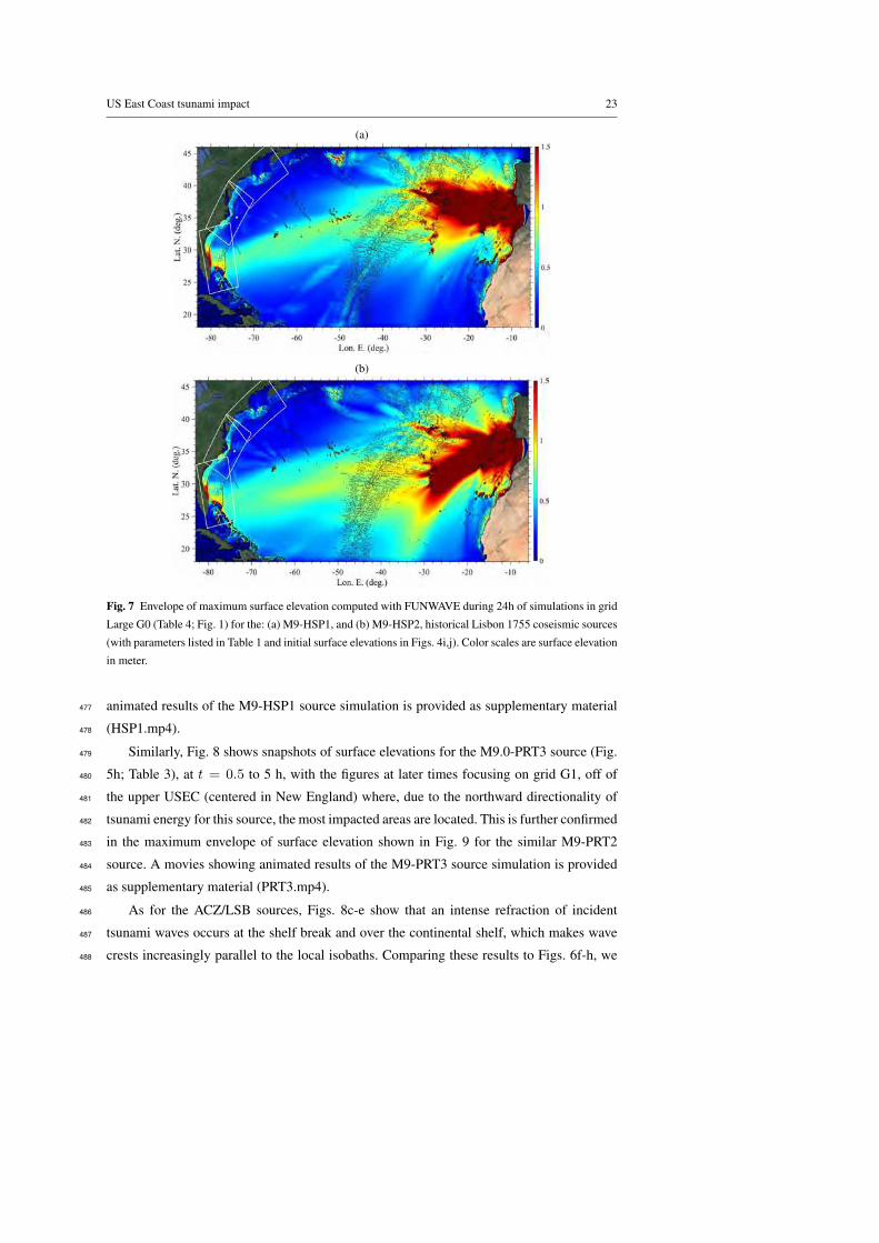
(a)
(b)
Fig. 7 Envelope of maximum surface elevation computed with FUNWAVE during 24h of simulations in grid
Large G0 (Table 4; Fig. 1) for the: (a) M9-HSP1, and (b) M9-HSP2, historical Lisbon 1755 coseismic sources
(with parameters listed in Table 1 and initial surface elevations in Figs. 4i,j). Color scales are surface elevation
in meter.
animated results of the M9-HSP1 source simulation is provided as supplementary material477
(HSP1.mp4).478
Similarly, Fig. 8 shows snapshots of surface elevations for the M9.0-PRT3 source (Fig.479
5h; Table 3), at t = 0.5 to 5 h, with the figures at later times focusing on grid G1, off of480
the upper USEC (centered in New England) where, due to the northward directionality of481
tsunami energy for this source, the most impacted areas are located. This is further confirmed482
in the maximum envelope of surface elevation shown in Fig. 9 for the similar M9-PRT2483
source. A movies showing animated results of the M9-PRT3 source simulation is provided484
as supplementary material (PRT3.mp4).485
As for the ACZ/LSB sources, Figs. 8c-e show that an intense refraction of incident486
tsunami waves occurs at the shelf break and over the continental shelf, which makes wave487
crests increasingly parallel to the local isobaths. Comparing these results to Figs. 6f-h, we488

24 Grilli et al.
(a) (b)
(c) (d)
(e) (f)
Fig. 8 Snapshots of surface elevations (color scale in meter) for the PRT/Caribbean arc source M9-PRT3
(Table 3; Fig. 5h), at t = (a) 0.5, (b) 2, (c) 3, (d) 4, (e) 4.5, and (f) 5 h. Some isobaths are plotted for
reference, but without labels to simplify the figures. Higher resolutions results are used wherever available.

US East Coast tsunami impact 25
Fig. 9 Envelope of maximum surface elevation computed with FUNWAVE during 24h of simulations in grid
Local G0 (Table 4; Fig. 1) for the M9-PRT3 coseismic source (with parameters listed in Table 3 and initial
surface elevations in Figs. 5h). Color scales are surface elevation in meter.
see that wave focusing-defocusing caused by refraction over the wide and shallow shelf,489
particularly around ridges and canyons in the bottom bathymetry, yields a corresponding490
modulation of tsunami coastal impact that is independent from the initial tsunami direction-491
ality. Detailed results of coastal impact, discussed later, will confirm that these modulation492
patterns are identical for the ACZ/LSB or PRT sources, which are originated eastward and493
southward, respectively. This leads to the same areas of the coast always being subjected494
to more or less tsunami hazard, whatever the tsunami source origin. This phenomenon was495
already noted in earlier work, for other tsunami sources affecting the USEC [27,54,45].496
Finally, for each source, the relevance of the one-way coupling method is verified by497
comparing time series of surface elevations at the 9 save points (Table 3.1), in the coarser498
grids Larger G0/Local G0 and the finer nested grids G1, G2 and G3. For instance, Figures499
10 and 11 show time series of surface elevations computed for the M9-HSP1 and M9.0-500
PRT1 sources. At most locations, there is a good agreement of the coarse and finer grid501
simulations for the first few hours of tsunami impact. Once reflected waves from the coast502
propagate back to the save points, however, differences become larger as reflection is more503
accurately computed in the finer grids. Differences are largest at point P-G1, which is on504
the shelf in shallower water and closer to shore, east of Cape Cod. Overall, the agreement505
of time series computed in different grids confirms the relevance of the one-way coupling506
methodology in nested grids used here. Time series of surface elevations at save points look507
qualitatively similar for the other ACZ/LSB and PRT sources and will not be repeated here.508

26 Grilli et al.
Fig. 10 Time series of surface elevations computed for the M9-HSP1 source (Table 1), at the 9 save points
defined in Table 5 (shown in Figs. 1): (blue lines) in grid Large G0; (red lines) in nested grids G1-G3. For
point P4, yellow indicates surface elevation computed in G2, red indicates surface elevation computed in G3.
4 Results of tsunami coastal impact509
4.1 Tsunami hazard metrics510
4.1.1 Definition of hazard metrics and classes511
For each of the ten ACZ/LSB (Table 1; Fig. 4 and eight PRT/Caribbean arc coseismic512
sources (Table 3; Fig. 5) simulated with FUNWAVE, coastal impact was computed in the513
three nested grids (G1, G2, G3) along the 5 m isobath that parallels the USEC (considering514
the coarse coastal grids used here). FUNWAVE results were interpolated at a large number515

US East Coast tsunami impact 27
Fig. 11 Time series of surface elevations computed for the M9-PRT3 source (Table 3), at the 9 save points
defined in Table 5 (shown in Figs. 1): (blue lines) in grid Local G0; (red lines) in nested grids G1-G3. For
point P4, black indicates surface elevation computed in G2, red indicates surface elevation computed in G3.
of coastal save points defined by their latitude-longitude coordinates along the isobath. For516
clarity, in most of the results and figures, J = 18, 201 save points are used, which exclude517
large bays (i.e., Cheasapeake and Delaware bays, and Long Island Sound); when large bays518
are considered, an additional 10,210 save points are specified within the bays (J = 28, 411).519
Based on these results, values of four tsunami hazard metrics Mi (i = 1, ..., 4) were com-520
puted for each source along the isobath: (1) maximum tsunami elevation M1 = ηmax, (2)521
current M2 = Umax, and (3) momentum force M3 = Fmax, as well as (4) M4 = 1/ta,522
function of arrival time ta (here a large arrival time corresponds to a low hazard). These523
metrics quantify inundation hazard, navigational hazard nearshore and in harbors, hazard524
28 Grilli et al.
(a) (b) (c) (d)
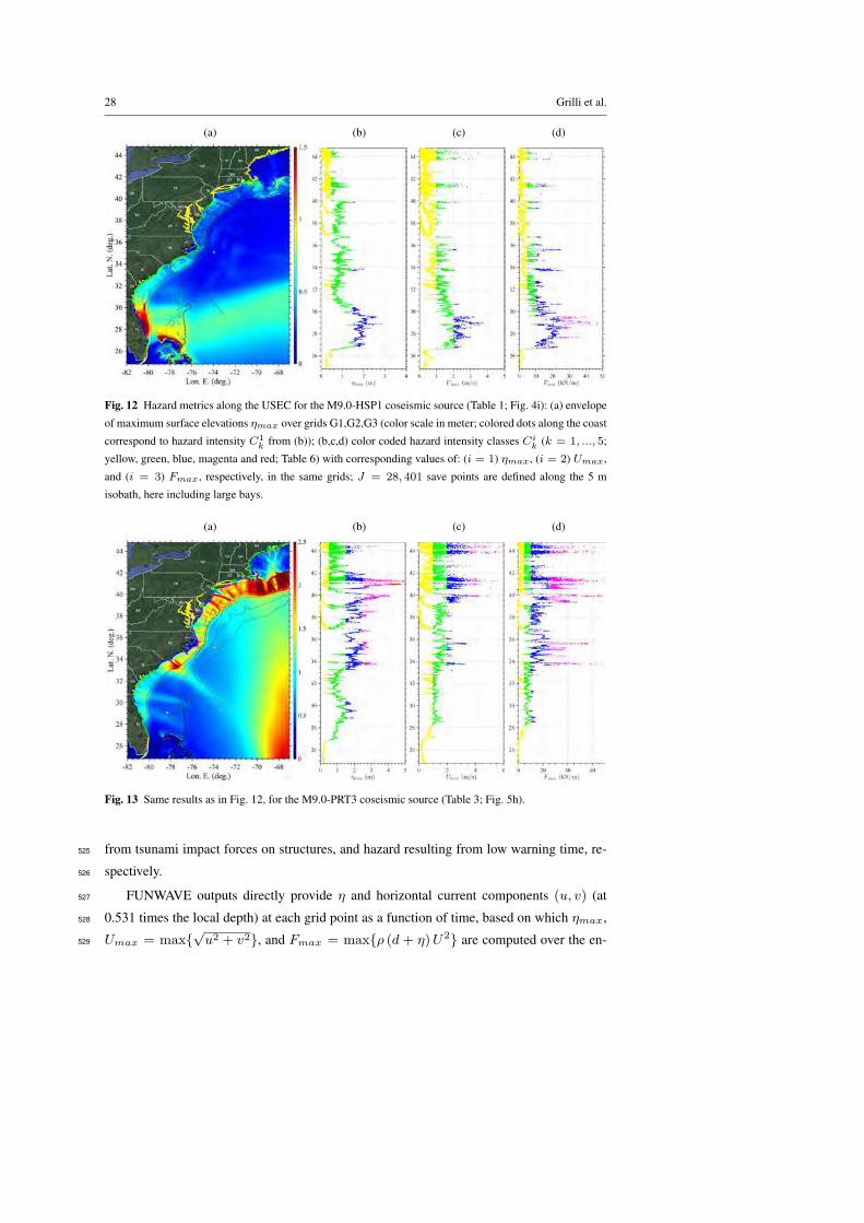
Fig. 12 Hazard metrics along the USEC for the M9.0-HSP1 coseismic source (Table 1; Fig. 4i): (a) envelope
of maximum surface elevations ηmax over grids G1,G2,G3 (color scale in meter; colored dots along the coast
correspond to hazard intensity C1
k from (b)); (b,c,d) color coded hazard intensity classes Cik (k = 1, ..., 5;
yellow, green, blue, magenta and red; Table 6) with corresponding values of: (i = 1) ηmax, (i = 2) Umax,
and (i = 3) Fmax, respectively, in the same grids; J = 28, 401 save points are defined along the 5 m
isobath, here including large bays.
(a) (b) (c) (d)
Fig. 13 Same results as in Fig. 12, for the M9.0-PRT3 coseismic source (Table 3; Fig. 5h).
from tsunami impact forces on structures, and hazard resulting from low warning time, re-525
spectively.526
FUNWAVE outputs directly provide η and horizontal current components (u, v) (at527
0.531 times the local depth) at each grid point as a function of time, based on which ηmax,528
Umax = max{√u2 + v2}, and Fmax = max{ρ (d + η)U2} are computed over the en-529

US East Coast tsunami impact 29
(a) (b) (c) (d)
Fig. 14 Envelope at the 5 m isobath (J = 18, 201 save points excluding large bays) of maximum tsunami:
(a) elevation; (b) current; (c) momentum force; and (d) arrival time, computed in grids G1,G2,G3, for the
ten ACZ/LSB sources (Table 1; Fig. 4): (green) M8.0-MTR1, M8.0-MTR2; (yellow) M8.3-MTR1, M8.3-
MTR2; (magenta) M8.7-MTR1, M8.7-MTR2; (red) M9.0-MTR1, M9.0-MTR2; and (black) M9.0-HSP1,
M9.0-HSP2. Note, arrival times for the latter two sources, which are slightly longer, are not shown for clarity.
tire duration of simulations at all grid point. Figures 7 and 9, show examples of maximum530
surface elevations computed over the entire computational domain for some of the tsunami531
sources. These results are then interpolated at the save points along the 5 m isobath. Tsunami532
arrival time is calculated along the same isobath, as the time when a positive or negative sur-533
face elevation first occurs over a threshold, i.e., ta (in hours) is the minimum time such that534
| η(ta, xj , yj) |≥ ∆η; where (xj , yj) (j = 1, ..., J) denotes the save points along the535
isobath and here ∆η = 0.01 m. Since tsunamis are very small amplitude waves relative536
to depth in most of their propagation, their celerity is well approximated as a function of537
depth by the linear long wave celerity, c =√gd, which is not amplitude dependent; hence538
different tsunamis originated from the same area propagate similarly along the same “wave539
rays”. This similarity of propagation to shore is further reinforced by refraction that takes540
place in large depth for long tsunami waves and causes each tsunami to propagate similarly541
over the wide USEC shelf, whatever its origin. Consequently, tsunamis of different mag-542
nitude originated from the same area, LSB/ACZ or PRT/Caribbean arc, should have very543
similar arrival times along the USEC, which will be verified in results. One caveat is, for the544
weakest LSB/ACZ M8 and M8.3 sources that approach areas of the USEC featuring bays545
and more complex shoreline geometries, with a small amplitude, and hence only reach the546

30 Grilli et al.
(a) (b) (c) (d)
Fig. 15 Envelope at the 5 m isobath (J = 18, 201 save points excluding large bays) of maximum tsunami: (a)
elevation; (b) current; (c) momentum force; and (d) arrival time, computed in grids G1,G2,G3, for the eight
PRT/Caribbean arc sources (Table 2.2; Fig. 5): (green) M8.3-PRT1, M8.3-PRT2, M8.3-PRT3; (magenta)
M8.7-PRT1, M8.7-PRT2; (red) M9.0-PRT2, M9.0-PRT2; and (black) M9.0-PRT3. Note, arrival times for the
latter source, which is similar, is not shown for clarity.
Hazard Metric Ci1
Ci2
Ci3
Ci4
Ci5
M1 = ηmax (m) [0-0.5[ [0.5-1.5[ [1.5-2.5[ [2.5-4[ > 4
M2 = Umax (m/s) [0-1[ [1-2[ [2-3.5[ [3.5-5[ > 5
M3 = Fmax (kN/m) [0-5[ [5-10[ [10-25[ [25-50[ > 50
M4 = 1/ta (1/h) [0-0.1[ [0.1-0.17[ [0.17-0.25[ [0.25-0.50[ > 0.50
Table 6 Class limits [Cik,min − Ci
k,max[, with (k = 1, ..., 5) of hazard intensity (low, low-medium,
medium, high, to highest hazard), for four hazard metrics Mi (i = 1, ..., 4) used to compute the Tsunami
Intensity Index (TII) with Eq. (3).
∆η threshold later in their propagation, due to shoaling and reflection of the tsunami wave547
trains. This tends to increase the arrival time for these sources in some areas. Details will be548
shown later.549
Once the four hazard metrics computed, to more easily identify areas facing lesser or550
larger hazard, similar to classes defined by Boschetti et al. [10] for the first two metrics in551
their tsunami intensity scale, we define five intensity classes, referred to as Cik; k = 1, ..., 5552
for each of the four metrics, with ranges of values [Cik,min−Ci
k,max[ from low to increasing553
hazard severity (Table 6). These classes of hazard for each metric can also be referred to as:554

US East Coast tsunami impact 31
low, low-medium, medium, high, and highest hazard. As discussed in Boschetti et al. [10],555
who reviewed other relevant work to date, the selected values for maximum inundation556
ηmax correspond, for adult pedestrians, to being up to knee-tight deep for class C1
1 , up557
to chest/head deep for class C1
2 , up to head to overhead deep for C1
3 while loosing the558
ability to feel the terrain, and then very deep; in classes C1
3 and higher, people would be559
forced to swim or have to find high ground or vertically evacuate to be safe. Likewise, for560
maximum currents Umax (see also Lynett et al. [38]), adult pedestrians would only be able561
to fight the current in classes C2
1 and C2
2 , while navigation would start being gradually562
and then severely impended nearshore and in harbors for classes C2
2 and above. Maximum563
momentum force Fmax classes correspond to most structures resisting up to most structures564
suffering significant damage or destruction, except for the strongest concrete or steel-built565
(also elevated) structures. Finally, regarding arrival time, the classes reflect going from large566
enough time (10 h) to evacuate most of the population from high hazard areas to not having567
enough time (2 h) for warning and evacuating a meaningful fraction of the population at568
risk. For each source considered here, and for their envelopes, values of the four metrics569
Mi were computed along the 5 m isobath and then sorted out by class. Plots of each metric570
along the isobath were made, which were color coded as a function of the corresponding571
class for the metric, Cik: yellow, green, blue, magenta, and red , for k = 1, 2, 3, 4, 5.572
4.1.2 Overall results of hazard metrics and classes573
Figures 12 and 13 show examples of results of the first 3, physical, metrics computed com-574
puted in grids G1,G2,G3, at J = 28, 401 save points on the 5 m isobath, here in includ-575
ing large bays, for the M9-HSP1 ACZ/LSB source (Table 1; Fig. 4i) and the M9.0-PRT3576
PRT/Caribbean arc source (Table 3; Fig. 5h). In each figure, panel (a) shows the envelope of577
maximum elevation, and panels (b,c,d) show the maximum elevation, current, and force, at578
the 5 m isobath, color-coded with their hazard class intensity Cik value; the class intensity579
value of surface elevation along is also marked in (a) along the coast.580
As for the envelope in grids Local/Large G0 shown in Figs. 7 and 9, we first observe581
an overall effect of the tsunami directionality on coastal impact, with the 15 deg. strike582
ACZ/LSB source (M9.0-HSP1) affecting more the lower USEC and the Caribbean Islands,583
and the PRT source (M9.0-PRT3) affecting more the upper USEC. Additionally, as before,584
for both sources, there is a fine scale modulation of tsunami impact along the USEC, as a585
function of the bathymetry (particularly on the shelf break and shelf) due to refraction caus-586
ing wave focusing/defocusing on specific areas of the coast with convex/concave isobath587
geometry, respectively. For both of these sources and for the three plotted metrics, there are588
many locations in the 3rd and 4th hazard class and a few in the 5th, highest hazard class for589

32 Grilli et al.
maximum elevation and current. This is expected and these are among the largest magni-590
tude sources. Computed results look qualitatively similar for the other, smaller magnitude,591
ACZ/LSB and PRT sources and will not be detailed here individually. However, their overall592
impact on the USEC is compared with each other next.593
Thus, Figs. 14 and 15 show a comparison of tsunami coastal impact at J = 18, 201594
save points along the 5 m isobath, here excluding large bays, for the four hazard metrics595
Mi, of the ten ACZ/LSB sources (Table 1) and eight PRT/Caribbean arc sources (Table 3),596
respectively. Tables 7 and 8 provide statistics computed based on these results, for the: mean,597
standard deviation, root-mean-square and average of the top 33, 10, 1 and 0.1 percentiles, of598
the first three metrics. For the 3 physical hazard metrics, results in Tables 7 and 8 show the599
expected trend of the statistics with the intensity of each metric statistics increasing with the600
source magnitude, except for 0.1 percentile results which only average 18 individual results601
and hence are more sensitive to a few noisy results. One exception is the two M9.0-HSP1602
and -HSP2 sources in the ACZ area, which due to the effect of the MTR, cause a slightly603
lower overall impact on the USEC than the two M9.0-MTR1 and -MTR2 sources which604
are sited west of the MTR. Due to sources’ directivity and refraction, the overall impact of605
ACZ/LSB sources in larger on the southern USEC (south of 35 deg. N), whereas it is the606
opposite for the PRT/Caribbean arc sources.607
Regarding the arrival time metric, Figs. 14d show, as expected, that all the arrival times608
are quite close to each other, ranging between 7.75 and 12.5 h, except for a few larger609
spurious values for the weakest ACZ sources. Note that overall, the M9 sources located610
further east in the HSP have an arrival time about 30 min larger than for the M9 sources611
located in the MTR. The arrival times for the ACZ/LZB sources are mostly in hazard class612
2, with a smaller fraction of values in hazard class 1. For the PRT sources, Fig. 15d shows613
that arrival times are shorter than for ACZ sources (2.5-7.25 h), but follow a similar pattern614
along the coast, due to the similar refraction over the wide shelf. The PRT arrival times are615
nearly the same for all sources (within a few minutes form each other) and fall mostly within616
the medium and high hazard classes (3 and 4).617
4.1.3 Detailed results of hazard metrics and classes618
For ACZ sources, results of the 3 physical metrics in Figs. 14a-c and in Table 7 show that619
the two M8.0 sources, which have 32 times less energy than the M9.0 sources (see Eq. 1),620
only cause a ∼ 0.03 m average maximum elevation along the USEC, with a 0.03 or 0.013621
m standard deviation, and the two M8.3 sources, which have 11 times less energy than the622
M9.0 sources, a ∼ 0.09 m average maximum elevation with a 0.07 standard deviation.623
Average maximum currents and forces are commensurate with these values and small for624

US East Coast tsunami impact 33
η (m) µη ση ηrms η1/3 η1/10 η1/100 η1/1000
M8.0-MTR1 0.032 0.031 0.044 0.053 0.079 0.205 0.637
M8.0-MTR2 0.025 0.013 0.028 0.040 0.054 0.072 0.085
M8.3-MTR1 0.091 0.068 0.113 0.161 0.230 0.438 0.975
M8.3-MTR2 0.085 0.061 0.104 0.148 0.217 0.369 0.7234
M8.7-MTR1 0.319 0.218 0.386 0.566 0.807 1.102 1.374
M8.7-MTR2 0.297 0.222 0.371 0.546 0.799 1.101 1.375
M9.0-MTR1 0.652 0.488 0.814 1.226 1.694 2.299 2.700
M9.0-MTR2 0.601 0.490 0.775 1.163 1.713 2.292 2.680
M9.0-HSP1 0.598 0.435 0.740 0.897 1.397 2.179 2.639
M9.0-HSP2 0.606 0.436 0.747 0.907 1.426 2.107 2.517
U (m/s) µU σU Urms U1/3 U1/10 U1/100 U1/1000
M8.0-MTR1 0.056 0.109 0.122 0.115 0.236 0.892 2.108
M8.0-MTR2 0.038 0.086 0.094 0.076 0.134 0.405 1.731
M8.3-MTR1 0.165 0.184 0.247 0.319 0.547 1.417 2.581
M8.3-MTR2 0.159 0.177 0.238 0.312 0.533 1.320 2.554
M8.7-MTR1 0.466 0.340 0.577 0.841 1.235 1.863 2.400
M8.7-MTR2 0.441 0.338 0.556 0.815 1.209 1.806 2.149
M9.0-MTR1 0.756 0.473 0.892 1.280 1.704 2.571 5.011
M9.0-MTR2 0.814 0.579 0.999 1.465 2.051 3.027 5.009
M9.0-HSP1 0.747 0.549 0.927 1.127 1.763 2.749 3.593
M9.0-HSP2 0.819 0.605 1.019 1.263 1.908 2.841 3.516
F (kN/m) µF σF Frms F1/3 F1/10 F1/100 F1/1000
M8.0-MTR1 0.024 0.199 0.200 0.063 0.176 1.295 4.919
M8.0-MTR2 0.010 0.205 0.206 0.027 0.067 0.373 3.033
M8.3-MTR1 0.159 0.375 0.407 0.397 0.880 3.280 4.501
M8.3-MTR2 0.134 0.234 0.270 0.335 0.695 1.476 2.749
M8.7-MTR1 1.374 2.209 2.601 3.360 6.634 14.065 23.618
M8.7-MTR2 1.285 2.116 2.476 3.202 6.447 13.277 19.043
M9.0-MTR1 3.576 4.636 5.855 8.307 15.277 24.486 36.386
M9.0-MTR2 4.051 5.528 6.853 9.798 17.688 30.455 42.936
M9.0-HSP1 3.788 5.796 6.924 6.722 14.539 31.737 55.390
M9.0-HSP2 4.424 6.029 7.477 7.929 16.093 30.003 49.653
Table 7 Statistics of simulation results computed at J = 18, 201 save points along the 5 m isobath (ex-
cluding large bays) for LSB/ASZ sources (Table 1; Fig. 14): mean, standard deviation, root-mean-square and
average of the top 33, 10, 1 and 0.1 percentiles of maximum elevation η (m), flow velocity U (m/s), and
momentum force F (kN/m).

34 Grilli et al.
η (m) µη ση ηrms η1/3 η1/10 η1/100 η1/1000
M8.3-PRT1 0.148 0.108 0.183 0.274 0.384 0.561 0.696
M8.3-PRT2 0.086 0.056 0.103 0.149 0.210 0.326 0.484
M8.3-PRT3 0.046 0.030 0.055 0.075 0.102 0.208 0.410
M8.7-PRT1 0.216 0.145 0.260 0.382 0.540 0.747 0.841
M8.7-PRT2 0.377 0.225 0.439 0.659 0.803 0.855 0.903
M9.0-PRT1 0.991 0.634 1.177 1.745 2.334 3.148 3.765
M9.0-PRT2 0.800 0.540 0.965 1.429 1.969 2.921 3.947
M9.0-PRT3 1.164 0.786 1.404 2.087 2.852 4.217 4.868
U (m/s) µU σU Urms U1/3 U1/10 U1/100 U1/1000
M8.3-PRT1 0.208 0.176 0.272 0.381 0.605 1.226 1.956
M8.3-PRT2 0.128 0.117 0.174 0.229 0.374 0.901 1.807
M8.3-PRT3 0.061 0.054 0.082 0.104 0.167 0.440 0.763
M8.7-PRT1 0.305 0.226 0.379 0.534 0.8123 1.512 2.277
M8.7-PRT2 0.530 0.341 0.630 0.904 1.276 2.035 2.562
M9.0-PRT1 1.232 0.719 1.426 2.005 2.820 4.111 4.938
M9.0-PRT2 1.120 0.905 1.440 2.009 3.188 6.232 7.688
M9.0-PRT3 1.255 0.748 1.461 2.062 2.862 4.604 6.602
F (kN/m) µF σF Frms F1/3 F1/10 F1/100 F1/1000
M8.3-PRT1 0.270 0.504 0.571 0.654 1.359 3.946 6.248
M8.3-PRT2 0.100 0.254 0.273 0.237 0.508 1.928 4.701
M8.3-PRT3 0.025 0.092 0.095 0.058 0.132 0.695 1.700
M8.7-PRT1 0.524 0.688 0.865 1.184 2.207 4.253 5.287
M8.7-PRT2 1.378 1.252 1.862 2.886 4.143 5.1682 5.776
M9.0-PRT1 9.060 10.937 14.202 19.289 34.444 76.255 107.810
M9.0-PRT2 6.995 10.026 12.225 16.012 30.981 65.731 92.363
M9.0-PRT3 9.914 10.950 14.771 21.291 35.827 63.969 108.922
Table 8 Statistics of simulation results computed at J = 18, 201 save points along the 5 m isobath (exclud-
ing large bays) for PRT sources (Table 2.2; Fig. 15): mean, standard deviation, root-mean-square and average
of the top 33, 10, 1 and 0.1 percentiles of maximum elevation η (m), flow velocity U (m/s), and momentum
force F (kN/m).
the most part, with currents being less than 2 knots (1 m/s) at all but a few locations (in 0.1625
percentile). Note that larger current (and corresponding force) values can result here from626
the coarse grid resolution and insufficient energy dissipation by bottom friction nearshore.627
Overall, statistics show that the physical metrics for the M8 and M8.3 sources cause a low628
to medium-low hazard. For elevation, only 0.1% of elevation values are in a hazard class629
higher than 1; 0.1% of current values are in a hazard class higher than 2, and 99.9% of the630
force values are in hazard class 1. For the larger ACZ sources, results in Figs. 14a-c and631
in Table 7 show that, as expected, the largest hazard for the first three metrics is caused632
by the four M9.0 sources, with many values falling in the high/highest hazard classes 4/5633

US East Coast tsunami impact 35
for each metric (Table 6). Among those, at many locations, slightly larger values of the634
three metrics are caused by the sources located west of the Madeira Torre Rise (MTR); but635
there are also locations where the sources located in the Horseshoe Plain (HSP) cause larger636
values. Looking at the detailed impact in the figures, South of 35.5 Lat. N. (approximately637
Cape Hatteras, NC), there are only small differences for the 3 metrics, between the sources638
located west of the MTR (M9-MTR1, M9-MTR2) and those east of it (M9-HSP1, M9-639
HSP2), with even some locations in the south where currents and forces are slightly larger640
for the latter two sources, indicating that here the Madeira Torre Rise (MTR) either does641
not affect tsunami propagation or reinforces it slightly. In contrast, north of 35 Lat. N. the642
tsunami hazard for the 3 metrics is larger for the M9 sources located west of the MTR643
than for the HSP sources, indicating that the shallow MTR ridge offers some protection644
from coseismic sources located in the area of the Lisbon 1755 event. Here, while maximum645
surface elevations reach similar maximum values as in the south, mostly in the high hazard646
category, currents and forces reach values in the highest hazard category at a larger number647
of locations.648
Regarding the medium-high magnitude M8.7 LSB/ACZ sources, results in Figs. 14a-c649
and in Table 7 for the three metrics show that, overall, these sources, which are about 3650
times less energetic than the M9 sources (see Eq. 1), cause less impact at most locations651
than the M9 sources, while following the same pattern of highs and lows along the coast as652
for the M9 sources. However, at some isolated locations in the south, maximum elevation653
reaches up to 1.9 m for the M8.7 sources and in the north, particularly above 39 Lat. N654
(about Atlantic City, NJ), at a few locations currents and forces reach values nearly as large655
as those of the M9-HSP1 and M9-HSP2 sources. Clearly, this results from the complex656
tsunami propagation from the source, including wave interactions with the MTR near the657
source and with bathymetry and coastal features along the USEC shelf break and shelf.658
Resonances (seiching) can also be triggered nearshore due to different frequency content659
in the incident wave train, that may increase currents even if tsunami elevations are not660
significantly affected.661
For PRT sources, Figs. 15a-c show that, as a result of refraction and an overall identical662
northward directivity of each PRT/Caribbean arc source, the impact of each source follows663
the same pattern of focusing/defocusing on the same coastal areas, with just a modulation of664
the intensity commensurate with the source magnitude. However, the overall intensity of the665
impact for the 3 physical metrics is 2-3 times smaller, south of 34 Lat. N. (approximately666
south of Cape Hatteras, NC), than north of it. So clearly the PRT/Caribbean arc sources667
mostly impact the areas less impacted by the ACZ/LSB sources.668
Results of the 3 physical metrics for the PRT/Caribbean arc sources in Figs. 15a-c and669
in Table 8 show that the three M8.3 sources, which have about 21 times less energy than670

36 Grilli et al.
the M9.0 sources (see Eq. 1), only cause a ∼ 0.05 − 0.15 m average maximum elevation,671
with a 0.03-0.011 m standard deviation, and 0.4-0.7 m for the 0.1 percentile values. The two672
M8.7 sources, which have 11 times less energy than the M9.0 sources, have a ∼ 0.22 −673
0.38 m average maximum elevation with a 0.15-0.23 m standard deviation, and 0.8-0.9 m674
for the 0.1 percentile values. Average maximum currents and forces for these sources are675
commensurate with these inundation values and small for the most part, with currents being676
less than 1.25 m/s (2.5 knots) at all but a few locations (in 0.1 percentile). Note that larger677
current (and corresponding force) values can again result from the coarse grid resolution and678
insufficient energy dissipation by bottom friction nearshore. Overall, statistics show that the679
physical metrics for the M8.3 and M8.7 sources cause a low to medium-low hazard. Only680
0.1% of maximum current values are in hazard class 3. Tsunami impact is more severe for681
the three larger M9 PRT sources. Despite resulting from quite different fault areas, results682
in Figs. 15a-c and in Table 8 show fairly similar overall impacts for the three M9 sources,683
with moderate average values of the 3 metrics. However, there is large alongshore variation684
of the metrics as confirmed by values in the two highest percentile (1 and 0.1 %), that all685
fall in hazard classes 4/5, i.e., high to highest impact. Among the three sources M9.0-PRT3,686
which was used as an extreme PMT source in earlier work, causes the maximum inundation687
and forces, but M9.0-PRT2 causes slightly larger maximum currents for the 0, 1 and 0.1688
percentile, all in the highest hazard category.689
4.2 tsunami Intensity Index (TII)690
To provide an overall indicator of tsunami hazard intensity along the USEC, values of the
five hazard classes, computed for each source along the 5 m isobath for the four metrics,
were combined into a Tsunami Intensity Index (TII). The TII is defined as a weighed av-
erage of the class index values, ki(xj , yj) = 0 to 5 (from low hazard to highest hazard),
interpolated for the four metrics Mi (i = 1, ..., 4) (Table 6), at each save point location
(xj , yj) (j = 1, ..., J), i.e.,
TII(xj , yj) =4∑
i=1
wiki(xj , yj) with ki(xj , yj) =
Mi(xj , yj)− Ck,min
Ck,max − Ck,min(3)
where wi are weights associated with each metric, with∑
i wi = 1, and the kis are com-691
puted by first finding the hazard class within which each metric falls and then applying Eq.692
(3). The TII hence is also on a scale of 0 to 5 and represents the overall tsunami hazard693
intensity, from low to highest. If all metrics are given equal weight then we simply have694
wi = 0.25; however, as we shall see, the weights allow giving more importance to some695
metrics than others.696
US East Coast tsunami impact 37
In the following, we elected to give more weight to variables directly affecting the ability697
of the population to evacuate, i.e., maximum inundation height and current, and relatively698
less weight to forces on structures and arrival time; thus, we gave weights of wi = [0.4, 0.3,699
0.15, 0.15] to each metric, respectively. The rationale for giving less weight to arrival time700
is that these are far-field coseismic tsunamis for which advanced warning would be imme-701
diately given upon the triggering of the event by an earthquake, hence somewhat mitigating702
this part of the hazard. However, any other combination of metric weights could be ap-703
plied and results easily generated. Figures 16 and 17 show the longshore distributions of TII704
values computed with these weights using Eq. (3), based on the four hazard metric results705
computed along the 5 m isobath for the LSB/ACZ (Fig. 14) and PRT/Caribbean arc (Fig. 15)706
sources, respectively. We see that the TII class values (which are color coded for different707
levels of hazard using the same color scheme as that of the hazard intensity classes) well708
summarize overall tsunami hazard and confirm the detailed observations made above on the709
individual hazard metrics results. The TII, however, provides a unique and simple indicator710
of the hazard intensity expected for each source at the many save points along the coast,711
that can be easily understood and used by emergency managers. Although these figures are712
plotted at large scale, all results produced can be easily zoomed into and/or imported into a713
GIS, to evaluate the hazard faced by any particular area or specific community.714
4.3 Estimating the effect of return period715
Although the complete PTHA of tsunami hazard along the USEC will be addressed in future716
work, the approximate return periods provided in Tables 2 and 3 for each of the 18 coseismic717
sources whose impact was modeled along the USEC, allow drawing some preliminary con-718
clusions as of the expected intensity of tsunami hazard for different return periods. Specif-719
ically, the values of the TII and four associated hazard metrics, computed for each source720
along the coast, provide a measure of the intensity of the tsunami hazard as a function of the721
event return period.722
Altogether, the sources simulated here cover an estimated range of return periods, Tr ∈723
[70−2, 130] years, with the low end being the M8 ACZ sources and the high end the M9.0-724
PRT3 extreme source. While detailed results of each tsunami metric can be extracted for any725
save point along the coast, here, we only consider the overall statistics of the three physical726
tsunami metrics, maximum elevation, current and force given in Tables 7 and 8, to estimate727
ranges of expected values as a function of Tr . Based on these statistics, for instance, we see728
that the expected 0.1 percentile values up to return periods of ∼ 100 years are a maximum729
inundation η1/1000 ∼ 0.7 m, maximum current U1/1000 ∼ 2 m/s, and maximum force730
F1/1000 ∼ 5 kN/m; up to ∼ 250 years, these values become 1.4 m, 2.4 m/s and 24 kN/m;731
38 Grilli et al.
up to ∼ 500 years, they become 2.6 m, 5.0 m/s and 55 kN/m; and up to ∼ 1, 000 years, they732
become 4 m, 7.7 m/s and 108 kN/m. Finally, up to ∼ 2, 000 years, maximum inundation733
approaches 5 m, while the other metrics stay at the same level.734
5 Conclusions735
We presented the methodology for and overall results of model simulations conducted to736
simulate tsunami hazard along the USEC from a collection of 18 far-field coseismic sources737
ranging in magnitude from M8 to M9. These include 10 sources located in the ACZ area,738
ranging from M8 to M9 magnitude, with some representing Lisbon 1755 proxy (repeat)739
events and 8 sources in the PRT/Caribbean arc area from M8.3 to M9 magnitude. Results740
provide a comprehensive picture at the regional scale (i.e., at a coarse grid resolution) of741
the intensity of coastal tsunami hazard expected from each source in terms of 4 hazard742
metrics computed along the 5 meter isobath: (1) the maximum tsunami elevation, (2) current743
and (3) force, as well as tsunami arrival time. These metrics are combined into a single744
Tsunami Intensity Index (TII), whose value allows identifying areas and infrastructure at745
greater hazard from coseismic tsunamis.746
The 18 sources have estimated return periods ranging approximately between 100 and747
2,000 years. For each source, the TII thus provides an overall tsunami hazard intensity748
along the USEC coast that allows both a comparison among sources and a quantification749
of tsunami hazard as a function of the source return period. The detailed values of each met-750
ric, both saved over the model grids and along the 5 m isobath, can help quantify tsunami751
hazard at any given coastal location in the 14 considered US coastal states, from Florida to752
Maine. These can also provide initial and boundary conditions to perform higher resolution753
inundation mapping simulations in areas identified as having a higher tsunami hazard.754
While earlier work only focused on the most extreme tsunami sources causing PMTs,755
whose return period was largely unknown, the present work covers a collection of sources756
to which approximate return periods are associated. Combined with other tsunami sources757
such as nearshore SMFs and far-field volcanic collapse into a logic tree, the 18 coseismic758
sources modeled here could thus contribute to future PTHA work along the USEC.759

US East Coast tsunami impact 39
(a) (b) (c) (d)
(e) (f) (g) (h)
(i) (j) (k) (l)

40 Grilli et al.
(m) (n) (o) (p)
(q) (r) (s) (t)
Fig. 16 Tsunami intensity index computed for ten LSB/ACZ sources (Table 1; Fig. 4), based on results of the
4 hazard metrics in Fig. 14: (a,b) M8.0-MTR1; (c,d) M8.0-MTR2; (e,f) M8.3-MTR1; (g,h) M8.3-MTR2; (i,j)
M8.7-MTR1; (k,l) M8.7-MTR2; (m,n) M9.0-MTR1; (o,p) M9.0-MTR2; (q,r) M9.0-HSP1; (s,t) M9.0-HSP2.
TII metric weights are wi = [0.40, 0.30, 0.15, 0.15], and color coded hazard intensity classes are: (yellow)
low; (green) medium low; (blue) medium (magenta) medium high, (red) heigh, and (black) extreme. Note,
for the last 2 sources, the TII is also provided within the large bays.
However, pending such PTHA work, the overall estimates made here of tsunami hazard760
intensity for several physical variables, as a function of the event return period, can help761
put in perspective the tsunami hazard faced by the USEC with that resulting from other762
more prominent natural disasters such as tropical cyclones. For the highest hazard areas763
(0.1 percentile), we find that tsunami hazard in the 100-500 year return period range is764
commensurate with that posed by category 3-5 tropical cyclones, taking into account the765
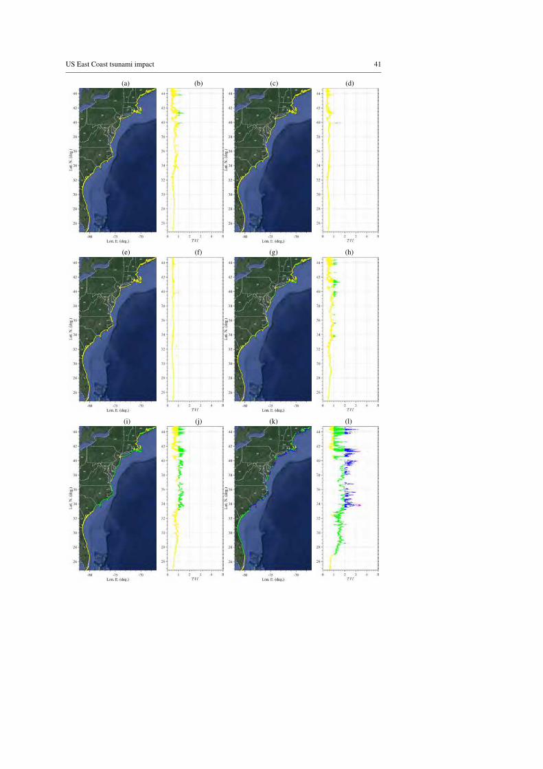
US East Coast tsunami impact 41
(a) (b) (c) (d)
(e) (f) (g) (h)
(i) (j) (k) (l)

42 Grilli et al.
(m) (n) (o) (p)
Fig. 17 Tsunami intensity index computed for eight PRT/Caribbean arc sources (Table 3; Fig. 5), based on
results of the 4 hazard metrics in Fig. 15: (a,b) M8.3-PRT1; (c,d) M8.3-PRT2; (e,f) M8.3-PRT3; (g,h) M8.7-
PRT1; (i,j) M8.7-PRT2; (k,l) M9.0-PRT1; (m,n) M9.0-PRT2; (o,p) M9.0-PRT3. TII metric weights are wi =
[0.40, 0.30, 0.15, 0.15], and color coded hazard intensity classes are: (yellow) low; (green) medium low;
(blue) medium (magenta) medium high, (red) heigh, and (black) extreme. Note, for the last source, the TII is
also provided within the large bays.
larger current velocities and forces caused by tsunami waves. Indeed, while the storm surge766
caused by category 3-5 hurricanes can reach 4-6 m along the USEC [58], the resulting767
coastal inundation is typically not associated with flow velocity and momentum forces as768
large as those caused by the long tsunami waves which, hence, could be more damaging769
even when associated with a smaller coastal inundation.770
Results of our work are made available to USEC emergency managers, who will be771
able to look at the most exposed areas to tsunami hazard and put the associated risk in772
perspective with that resulting from other natural disasters and implement the necessary773
mitigation measures.774
6 Declarations775
6.1 Funding776
This work was supported in the United States by NOAA’s National Weather Service (NWS),777
through grants administered by the US National Tsunami Hazards Mitigation Program (NTHMP):778
NA-13-NWS4670014, NA-14-NWS4670041, NA-15-NWS4670029, NA-16-NWS4670034,779
NA-17-NWS4670010, NA-18-NWS4670073 and NA-19-NWS4670074. Numerical simula-780
tions reported in this work used HPC resources, as part of the Extreme Science and Engi-781

US East Coast tsunami impact 43
neering Discovery Environment (XSEDE) (project BCS-170015), which is supported by the782
National Science Foundation (NSF) grant number ACI-1548562.783
6.2 Conflicts of interest/Competing interests784
None785
6.3 Availability of data and material (data transparency)786
A Google Drive repository for all the raw data that was used to set up the tsunami models and787
model results has been created. This is in fact a requirement of the NTHMP program. The788
Google Drive will be finalize and made public once the paper is accepted for publication.789
Note that the raw data does not provide any useful information in itself regarding.790
6.4 Code availability791
FUNWAVE-TVD, the tsunami model used in this work, is open source software available at792
http://github.com/fengyanshi/FUNWAVE-TVD/.793
6.5 Authors’ contributions794
SG: Led work, acquired funding, defined methodology, processed results and wrote most of795
the paper.796
MM: Performed model simulations, did background literature work, post processed results,797
made some figures and proofread paper.798
LS: Created model grids and performed model simulations for a few extreme sources, did799
background literature work, developed post-processing routines, and did some post process-800
ing of results.801
AG: Co-led work, helps to acquire funding, defined some of the methodology, performed802
early tsunami simulations and developed initial post-processing routines, proofread paper.803
6.6 Ethics approval804
Not applicable.805

44 Grilli et al.
6.7 Consent to participate806
Not applicable.807
6.8 Consent for publication808
Not applicable809
Acknowledgements The authors gratefully acknowledge continuing support from NOAA’s National Weather810
Service (NWS), through grants administered by the US National Tsunami Hazards Mitigation Program811
(NTHMP): NA-13-NWS4670014, NA-14-NWS4670041, NA-15-NWS4670029, NA-16-NWS4670034, NA-812
17-NWS4670010, NA-18-NWS4670073 and NA-19-NWS4670074. Numerical simulations reported in this813
work used HPC resources, as part of the Extreme Science and Engineering Discovery Environment (XSEDE)814
(project BCS-170015), which is supported by the National Science Foundation (NSF) grant number ACI-815
1548562. FUNWAVE-TVD is open source software available at http://github.com/fengyanshi/FUNWAVE-816
TVD/.817
References818
1. Abadie S., Harris J.C., Grilli S.T. and R. Fabre, Numerical modeling of tsunami waves generated by the819
flank collapse of the Cumbre Vieja Volcano (La Palma, Canary Islands): tsunami source and near field820
effects, Journal of Geophysical Research, 117, C05030, doi:10.1029/2011JC007646 (2012)821
2. Baptista, M. A., Heitor, S., Miranda, J.M., Miranda, P.M.A. and Mendes Victor, L., The 1755 Lisbon822
earthquake; evaluation of the tsunami parameters, J. Geodynamics, 25, 143-157 (1998a)823
3. Baptista, M. A., Heitor, S., Miranda, J.M., Miranda, P.M.A. and Mendes Victor, L., Constraints on the824
source of the 1755 Lisbon tsunami inferred from numerical modeling of historical data on the source of the825
1755 Lisbon tsunami, J. Geodynamics, 25, 159-174 (1998b)826
4. Baptista, M.A., Miranda, J. M., Chierici, F. and Zitellini, N., New study of the 1755 earthquake source827
based on multi-channel seismic survey data and tsunami modeling, Nat. Haz. Earth Syst. Sc., 3, 333-340828
(2003)829
5. Baptista, M. A. And Miranda, J. M., Revision of the Portuguese catalog of tsunamis. Natural Hazards and830
Earth System Sciences, 9(1), 25-42 (2009)831
6. Baptista, M. A., Miranda, J. M., Batllo, J., Lisboa, F., Luis, J., and Macia?, R., New study on the 1941832
Gloria Fault earthquake and tsunami. Natural Hazards and Earth System Sciences, 16(8), 1967-1977 (2016)833
7. Baptista, M.A., 2020, Tsunamis Along the Azores Gibraltar Plate Boundary. Pure and Applied Geo-834
physics, 177, 1713-1724 (2020)835
8. Barkan, R., ten Brick, U.S. and Lin, J., Far field tsunami simulations of the 1755 Lisbon earthquake:836
Implication for tsunami hazard to the U.S. East Coast and the Caribbean, Marine Geology, 264, 109-122837
(2009)838
9. Benford, B., DeMets, C., Calais, E. GPS estimates of microplate motions, northern Caribbean: evidence839
for a Hispaniola microplate and implications for earthquake hazard. Geophys. J. Intl., 191(2), 481-490,840
doi:10.1111/j.1365-246X.2012.05662.x (2012)841

US East Coast tsunami impact 45
10. Boschetti L., Ioualalen M., Nemati F., Grilli S.T., Dessa J.-X., and C. Larroque, Tsunami intensity scale842
based on wave amplitude and current applied to the French Riviera: the case study of local seismicity. Nat.843
Hazards, 102, 219-248, doi: 10.1007/s11069-020-03921-0 (2020)844
11. Calais, E. And Mercier de Lepinay. B. Strike-slip tectonic processes in the northern Caribbean between845
Cuba and Hispaniola (Windward Passage). Mar. Geophys. Res., 17(1), 63-95 (1995)846
12. Calais, E., Freed, A., Mattioli, G., Amelung, F., Jonsson, S., Jansma, P., Hong, S-H., Dixon, T., Prepetit,847
C. and Momplaisir, R. Transpressional rupture of an unmapped fault during the 2010 Haiti earthquake. Nat.848
Geoscience, 3(11), 749-799, doi:10.1038/NGEO992 (2010)849
13. Chaytor J.D., ten Brink U.S., Solow A.R., and B.D. Andrews, Size distribution of submarine landslides850
along the U.S. Atlantic margin. Marine Geology, 264(1-2):16-27 (2009)851
14. Dawicki, S., Major Caribbean Earthquakes and Tsunamis a Real Risk: Events rare, but scientists call852
for public awareness, warning system, Media Relations, Woods Hole Oceanographic Institute, available at:853
http://www.whoi.edu/page.do?pid=12460&tid=282&cid=2430 (last access: 13 December 2008 (2005)854
15. DeMets, C., Earthquake slip vectors and estimates of present-day plate motions. J. Geophys. Res., 98,855
6703-6714 (1993).856
16. Gailler, A., Calais, E., Hebert, H., Roy, C., Okal, E. Tsunami scenarios and hazard assessment along the857
northern coast of Haiti. Geophys. J. Intl., 203(3), 2287-2302, doi:10.1093/gji/ggv428 (2015)858
17. Gica, E., M. C. Spillane, V. V. Titov, C. D. Chamberlin, and J. Newman, Development of the forecast859
propagation database for NOAA’s Short-Term Inundation Forecast for Tsunamis, NOAA Tech. Memo.,860
OAR PMEL-139 (2008)861
18. Glimsdal S., Pedersen G.K., Harbitz C.B., and F. Løvholt, Dispersion of tsunamis: does it really matter862
?, Nat. Hazards Earth Syst. Sci., 13, 1507-1526, doi:10.5194/nhess-13-1507-2013 (2013)863
19. Grilli A.R. and S.T. Grilli, Modeling of tsunami generation, propagation and regional impact along864
the U.S. East Coast from the Azores Convergence Zone, Research Report no. CACR-13-04, 20 pps.,865
http://personal.egr.uri.edu/grilli//grilli-grilli-cacr-13-04 (2013a)866
20. Grilli A.R. and S.T. Grilli, Modeling of tsunami generation, propagation and regional impact along867
the upper U.S East coast from the Puerto Rico trench, Research Report no. CACR-13-02, 18 pps.,868
http://personal.egr.uri.edu/grilli//grilli-grilli-cacr-13-02 (2013b)869
21. Grilli, S.T., Grilli A.R., David, E. and C. Coulet, Tsunami Hazard Assessment along the North870
Shore of Hispaniola from far- and near-field Atlantic sources. Natural Hazards, 82(2), 777-810, doi:871
10.1007/s11069-016-2218-z (2016)872
22. Grilli S.T., Ioualalen M., Asavanant J., Shi F., Kirby J.T., and P. Watts, Source constraints and model873
simulation of the December 26, 2004 Indian Ocean tsunami, Journal of Waterway, Port, Coastal, and874
Ocean Engineering, 33, 414-428 (2007)875
23. Grilli S.T., Dubosq S., Pophet N., Perignon Y., Kirby J.T., and F. Shi, Numerical simulation and first-876
order hazard analysis of large coseismic tsunamis generated in the Puerto Rico thrench: near-field impact877
on the North shore of Puerto Rico and far-field impact on the US East Coast, Natural Hazards and Earth878
System Sciences, 10, 2109-2125, doi:10.5194/nhess-2109-2010 (2010)879
24. Grilli, S.T., J.C. Harris, T. Tajalibakhsh, T.L. Masterlark, C. Kyriakopoulos, J.T., Kirby and F. Shi Numer-880
ical simulation of the 2011 Tohoku tsunami based on a new transient FEM coseismic source: Comparison881
to far- and near-field observations, Pure Appl. Geophys., 170, 1333-1359, doi:10.1007/s00024-012-0528-y882
(2013c)883
25. Grilli S.T., O’Reilly C., Harris J.C., Tajalli-Bakhsh T., Tehranirad B., Banihashemi S., Kirby J.T., Baxter884
C.D.P., Eggeling T., Ma G. and F. Shi, Modeling of SMF tsunami hazard along the upper US East Coast:885
Detailed impact around Ocean City, MD, Natural Hazards, 76(2), 705-746, doi: 10.1007/s11069-014-886
1522-8 (2015)887

46 Grilli et al.
26. Grilli S.T., D.R. Tappin, S. Carey, S.F.L. Watt, S.N. Ward, A.R. Grilli, S.L. Engwell, C. Zhang, J.T. Kirby,888
L. Schambach and M. Muin, Modelling of the tsunami from the December 22, 2018 lateral collapse of Anak889
Krakatau volcano in the Sunda Straits, Indonesia, Scientific Reports, 9, 11946, doi:10.1038/s41598-019-890
48327-6 (2019)891
27. Grilli, S.T., Shelby, M., Kimmoun, O., Dupont, G., Nicolsky, D., Ma, G., Kirby, J. and F. Shi, Modeling892
coastal tsunami hazard from submarine mass failures: effect of slide rheology, experimental validation,893
and case studies off the US East coast, Natural Hazards, 86(1), 353-391, doi:10.1007/s11069-016-2692-3894
(2017)895
28. Harbitz, C.B., Glimsdal S., Bazin S., Zamora N., Løvholt F., Bungum H., Smebye H., Gauer P., and Kjek-896
stad O., Tsunami hazard in the Caribbean: Regional exposure derived from credible worst case scenarios,897
Continental Shelf Res., 8, 1-23, doi:10.1016/j.csr.2012.02.006 (2012)898
29. Horrillo J., Grilli S.T., Nicolsky D., Roeber V., and J. Zhang, Performance bench- marking tsunami899
models for NTHMP’s inundation mapping activities, Pure and Applied Geophysics, 172(3-4), 869-884900
(2015)901
30. Ioualalen M., Asavanant J., Kaewbanjak N., Grilli S.T., Kirby J.T. and P. Watts, Modeling the 26th902
December 2004 Indian Ocean tsunami: Case study of impact in Thailand, J. Geophys. Res., 112, C07024,903
doi:10.1029/2006JC003850 (2007)904
31. Kirby J.T., Shi F., Tehranirad B., Harris J.C. and S.T. Grilli, Dispersive tsunami waves in the905
ocean: Model equations and sensitivity to dispersion and Coriolis effects, Ocean Modell., 62, 39-55,906
doi:10.1016/j.ocemod.2012.11.009 (2013)907
32. Knight, B., Model predictions of Gulf and Atlantic Coast tsunami impacts from a distribution of sources,908
Science of Tsunami Hazard, 24(5), 304-312 (2006)909
33. Lander, J.F., Caribbean Tsunamis: an initial history, Nat. Haz., 3, 1-18 (1997)910
34. Lockridge, P.A., Whiteside, L.S. And J.F. Lander, Tsunamis and tsunami-like waves of the eastern United911
States, Science of Tsunami Hazards, 20(3), 120-157 (2002).912
35. Lopez-Venegas, A.M., Horrillo, J., Pampell-Manis, A., Huerfano, V., Mercado, A. Advanced tsunami913
numerical simulations and energy considerations by use of 3D-2D coupled models: the October 11, 1918914
Mona passage tsunami. Pure Appl. Geophys., 172(6), 1679-1698, doi:10.1007/s00024-014-0988-3 (2015).915
36. Løvholt, F., Pedersen, G. And G. Gisler, Oceanic propagation of a potential tsunami from the La Palma916
Island, Journal of Geophysical Research: Oceans, 113(C9) (2008)917
37. Løvholt, F., Schulten, I., Mosher, D., Harbitz, C. And S. Krastel, Modelling the 1929 Grand918
Banks slump and landslide tsunami, Geological Society, London, Special Publications, 477(1), 315-331,919
https://doi.org/10.1144/SP477.28 (2019)920
38. Lynett, P., and 37 alii, Inter-Model Analysis of Tsunami-Induced Coastal Currents, Ocean Modell., 114,921
14-32, doi:10.1016/j.ocemod.2017.04.003 (2017)922
39. Madsen P.A., D.R. Fuhrman and H. A. Schaffer, On the solitary wave paradigm for tsunamis. J.923
Geophys. Res., 113, C12012 (2008)924
40. Mercado, A. And W. McCann, Numerical simulation of the 1918 Puerto Rico tsunami, Natural Hazards,925
18(1), 57-76 (1998)926
41. Muir-Wood, R. And A. Mignan, A phenomenological reconstruction of the Mw9 November 1st 1755927
earthquake source, In The 1755 Lisbon Earthquake: Revisited, pp. 121-146, Springer, Dordrecht, (2009)928
42. Nemati F., Grilli S.T., Ioualalen M., Boschetti L., Larroque L. and J. Trevisan, High-resolution coastal929
hazard assessment along the French Riviera from coseismic tsunamis generated in the Ligurian fault sys-930
tem. Nat. Hazards, 96(2), 553-586, doi:10.1007/s11069-018-3555-x (2019)931
43. Okada, Y., Surface deformation due to shear and tensile faults in a half space, Bull. Seismol. Soc.932
America, 75(4), 1135-1154 (1985)933

US East Coast tsunami impact 47
44. Omira, R., Baptista, M. A., Matias, L., Miranda, J. M., Catita, C., Carrilho, F., et al., Design of a sea-934
level tsunami detection network for the Gulf of Cadiz. Natural Hazards and Earth System Sciences, 9(4),935
1327?1338 (2009)936
45. Schambach L., Grilli S.T., Kirby J.T. and F. Shi Landslide tsunami hazard along the upper US East937
Coast: effects of slide rheology, bottom friction, and frequency dispersion, Pure Appl. Geophys., 176(7),938
3,059-3,098, doi:10.1007/s00024-018-1978-7 (2019)939
46. Schambach L., Grilli S.T., Tappin D.R., Gangemi M.D., and G. Barbaro, New simulations and under-940
standing of the 1908 Messina tsunami for a dual seismic and deep submarine mass failure source, Marine941
Geology, 421, 106093, doi: 10.1016/j.margeo.2019.106093 (2020)942
47. Schambach L., Grilli S.T., Tappin D.R., New high-resolution modeling of the 2018 Palu tsunami, based943
on supershear earthquake mechanisms and mapped coastal landslides, supports a dual source, Frontiers in944
Earth Sciences, 8, 627, doi:0.3389/feart.2020.598839 (2020)945
48. Schambach, L., Grilli, S.T. and A.R. Grilli. Simulation of Global Tsunami Hazard along the U.S.946
East Coast. Research Report no. CACR-20-02. NTHMP Award, #NA18NWS4670073, National Weather947
Service Program Office, 93 pps., http://personal.egr.uri.edu/grilli/EC hazard report NTHMP CACRo.pdf948
(2020).949
49. Schnyder J.S., Eberli G. P., Kirby J.T., Shi F., Tehranirad B., Mulder T., Ducassou E., Hebbeln D., and950
Wintersteller P., Tsunamis caused by submarine slope failures along western Great Bahama Bank. Scientific951
Reports, 6, 35925 (2016)952
50. Shi F., Kirby J.T., Harris J.C., Geiman J.D., and S.T. Grilli, A high-order adaptive time-stepping TVD953
solver for Boussinesq modeling of breaking waves and coastal inundation, Ocean Modell., 43-44, 36-51,954
doi:10.1016/j.ocemod.2011.12.004 (2012)955
51. Tappin D.R., Watts P. and S.T. Grilli, The Papua New Guinea tsunami of 1998: anatomy of a catastrophic956
event, Natural Hazards and Earth System Sciences, 8, 243-266 (2008)957
52. Tappin D.R., Grilli S.T., Harris J.C., Geller R.J., Masterlark T., Kirby J.T., F. Shi, G. Ma, K.K.S. Thing-958
baijamg, and P.M. Maig (2014) Did a submarine landslide contribute to the 2011 Tohoku tsunami ? Marine959
Geology, 357:344-361 doi: 10.1016/j.margeo.2014.09.043960
53. Tehranirad B., Shi F., Kirby, J.T., Harris J.C. and S.T. Grilli, Tsunami benchmark results for fully961
nonlinear Boussinesq wave model FUNWAVE-TVD, Version 1.0, Technical report, No. CACR-11-02,962
Center for Applied Coastal Research, University of Delaware (2011)963
54. Tehranirad B., Harris J.C., Grilli A.R., Grilli S.T., Abadie S., Kirby J.T. and F. Shi, Far-field tsunami964
hazard in the north Atlantic basin from large scale flank collapses of the Cumbre Vieja volcano, La Palma,965
Pure Appl. Geophys., 172(12), 3,589-3,616, doi:10.1007/s00024-015-1135-5 (2015)966
55. ten Brink, U., Twichell D., Geist E., Chaytor J., Locat J., Lee H., Buczkowski B., Barkan R., Solow967
A., Andrews B., Parsons T., Lynett P., Lin J., and M. Sansoucy, Evaluation of tsunami sources with the968
potential to impact the U.S. Atlantic and Gulf coasts, USGS Administrative report to the U.S. Nuclear969
Regulatory Commission, 300 pp (2008)970
56. ten Brink, U.S., Bakun W.H. and Flores C.H., Historical perspective on seismic hazard to Hispaniola971
and the northeast Caribbean region, J. Geophys. Res. (Solid Earth), 106(B12) (2011)972
57. ten Brink, U.S., Chaytor, J.D., Geist, E.L., Brothers, D.S. and B.D. Andrews, Assessment of tsunami973
hazard to the US Atlantic margin, Marine Geology, 353, 31-54 (2014)974
58. Torres M.J., Hashemi, M.R., Hayward S., Spaulding M.L., Ginis I. and S.T. Grilli. Role of hurricane975
wind models in accurate simulation of storm surge and waves. J. Waterways, Port, Coastal Engng., 145(1),976
04018039 (2019)977
59. Udias, A., Large Earthquakes and Tsunamis at Saint Vincent Cape before the Lisbon 1755 Earthquake:978
A Historical Review. Pure and Applied Geophysics, 177, 1739-1745 (2020)979

48 Grilli et al.
60. Watts P., Grilli S.T., Kirby J.T., Fryer G.J. and D.R. Tappin, Landslide tsunami case studies using a980
Boussinesq model and a fully nonlinear tsunami generation model, Natural Hazards and Earth System981
Sciences, 3, 391-402 (2003)982
61. Wei G., Kirby J.T., Grilli S.T. and R. Subramanya, A fully nonlinear Boussinesq model for free surface983
waves. Part I: Highly nonlinear unsteady waves, Journal of Fluid Mechanics, 294, 71-92 (1995)984
62. Zahibo, N. and Pelinovsky, E. N., Evaluation of tsunami risk in the Lesser Antilles, Nat. Hazards Earth985
Syst. Sci., 1, 221-231, doi:10.5194/nhess-1-221-2001 (2001)986

Figures
Figure 1
Footprint and ETOPO1 bathymetry/topography (color scale in meter shows <> 0) of FUNWAVE’s 1 arc-minresolution grids in North Atlantic Ocean basin (Local/Large G0), with footprints of 3 regional 450 mnested shore-parallel Cartesian grids (G1, G2, G3; Table 4). Location are marked for the two areas ofhistorical/hypothetical tsunami coseismic sources (red oval) considered, near the Ac¸ores ConvergenceZone (ACZ), including Lisbon 1755 (LSB), and near and around the Puerto Rico Trench (PRT). TheMadeira Torre Rise (MTR) is the shallower ridge located on the north of the ACZ circled area and theHorseshoe Plain is to the East of the ACZ and MTR. Yellow/red symbols within the regional grids marklocations of numerical wave gauge stations where time series of surface elevation are calculated insimulations for validating the one-way grid coupling (Table 2). Note: The designations employed and thepresentation of the material on this map do not imply the expression of any opinion whatsoever on thepart of Research Square concerning the legal status of any country, territory, city or area or of itsauthorities, or concerning the delimitation of its frontiers or boundaries. This map has been provided bythe authors.

Figure 2
Likeliest segmentation in 5 segments of the PRT/Caribbean arc, from west of Hispaniola to Guadeloupein the eastern part, established at the May 2019 workshop of experts at the USGS Powell Center (see Fig.1 for location). Insert shows footprints of SIFT subfaults [17] in the considered area (see Table 2 forparameter values). Large black arrows show the nearly E-W relative plate motion of the North AmericaPlate subducting under the Caribbean Plate. Note: The designations employed and the presentation ofthe material on this map do not imply the expression of any opinion whatsoever on the part of ResearchSquare concerning the legal status of any country, territory, city or area or of its authorities, or concerningthe delimitation of its frontiers or boundaries. This map has been provided by the authors.

Figure 3
Footprints of 450 m resolution grids used in FUNWAVE, in spherical (left) and Cartesian (right)coordinates (Table 4, Fig. 1): (a) G1, (b) G2, (c) G3; color scales and contours are bathymetry/topographyin meter. Note: The designations employed and the presentation of the material on this map do not implythe expression of any opinion whatsoever on the part of Research Square concerning the legal status of

any country, territory, city or area or of its authorities, or concerning the delimitation of its frontiers orboundaries. This map has been provided by the authors.
Figure 4
Initial surface elevations computed with Okada’s [43] method (color scale in meter) for coseismic tsunamisources in the ACZ/LSB area (Fig. 1; Table 1) : (a) M8.0-MTR1; (b) M8.0-MTR2; (c) M8.3-MTR1; (d) M8.3-MTR2; (e) M8.7-MTR1; (f) M8.7-MTR2; (g) M9.0-MTR1; (h) M9.0-MTR2; (i) M9.0-HSP1; (j) M9.0-HSP2.

Each source has a single fault plane with footprint marked by white solid lines. Note, the M9.0 sourcesrepresent Lisbon 1755 proxies, located in either the ACZ, west of the MTR (”MTR”), or Horseshoe Plain(”HSP”) areas (Fig. 1.)
Figure 5
Initial surface elevations computed with Okada’s [43] method for the modeled PRT/Caribbean arctsunami sources (Fig. 1; Table 3): (a) M8.3-PRT1; (b) M8.3-PRT2; (c) M8.3-PRT3; (d) M8.7-PRT1; (e) M8.7-

PRT2; (f) M9.0-PRT1; (g) M9.0-PRT2; and (h) M9.0-PRT3. All source parameters are given Tables 2 and 3.Color scale (in meter), with same scale is used in plots (b-h), for comparison. Note: The designationsemployed and the presentation of the material on this map do not imply the expression of any opinionwhatsoever on the part of Research Square concerning the legal status of any country, territory, city orarea or of its authorities, or concerning the delimitation of its frontiers or boundaries. This map has beenprovided by the authors.
Figure 6

Snapshots of surface elevations (color scale in meter) computed for the Lisbon 1755 proxy source M9-HSP1 (Fig. 4i; Table 1), at t = (a) 1, (b) 2, (c) 5, (d) 6.5, (e) 8, (f) 9.5, (g) 10.5, and (h) 11 h. Some isobathsare plotted for reference, but without labels to simplify the �gures. Higher resolutions results are usedwherever available. Note: The designations employed and the presentation of the material on this map donot imply the expression of any opinion whatsoever on the part of Research Square concerning the legalstatus of any country, territory, city or area or of its authorities, or concerning the delimitation of itsfrontiers or boundaries. This map has been provided by the authors.
Figure 7

Envelope of maximum surface elevation computed with FUNWAVE during 24h of simulations in gridLarge G0 (Table 4; Fig. 1) for the: (a) M9-HSP1, and (b) M9-HSP2, historical Lisbon 1755 coseismicsources (with parameters listed in Table 1 and initial surface elevations in Figs. 4i,j). Color scales aresurface elevation in meter.
Figure 8

Snapshots of surface elevations (color scale in meter) for the PRT/Caribbean arc source M9-PRT3 (Table3; Fig. 5h), at t = (a) 0.5, (b) 2, (c) 3, (d) 4, (e) 4.5, and (f) 5 h. Some isobaths are plotted for reference, butwithout labels to simplify the �gures. Higher resolutions results are used wherever available. Note: Thedesignations employed and the presentation of the material on this map do not imply the expression ofany opinion whatsoever on the part of Research Square concerning the legal status of any country,territory, city or area or of its authorities, or concerning the delimitation of its frontiers or boundaries. Thismap has been provided by the authors.
Figure 9
Envelope of maximum surface elevation computed with FUNWAVE during 24h of simulations in gridLocal G0 (Table 4; Fig. 1) for the M9-PRT3 coseismic source (with parameters listed in Table 3 and initialsurface elevations in Figs. 5h). Color scales are surface elevation in meter. Note: The designationsemployed and the presentation of the material on this map do not imply the expression of any opinionwhatsoever on the part of Research Square concerning the legal status of any country, territory, city or

area or of its authorities, or concerning the delimitation of its frontiers or boundaries. This map has beenprovided by the authors.
Figure 10
Time series of surface elevations computed for the M9-HSP1 source (Table 1), at the 9 save pointsde�ned in Table 5 (shown in Figs. 1): (blue lines) in grid Large G0; (red lines) in nested grids G1-G3. For

point P4, yellow indicates surface elevation computed in G2, red indicates surface elevation computed inG3.
Figure 11
Time series of surface elevations computed for the M9-PRT3 source (Table 3), at the 9 save pointsde�ned in Table 5 (shown in Figs. 1): (blue lines) in grid Local G0; (red lines) in nested grids G1-G3. For
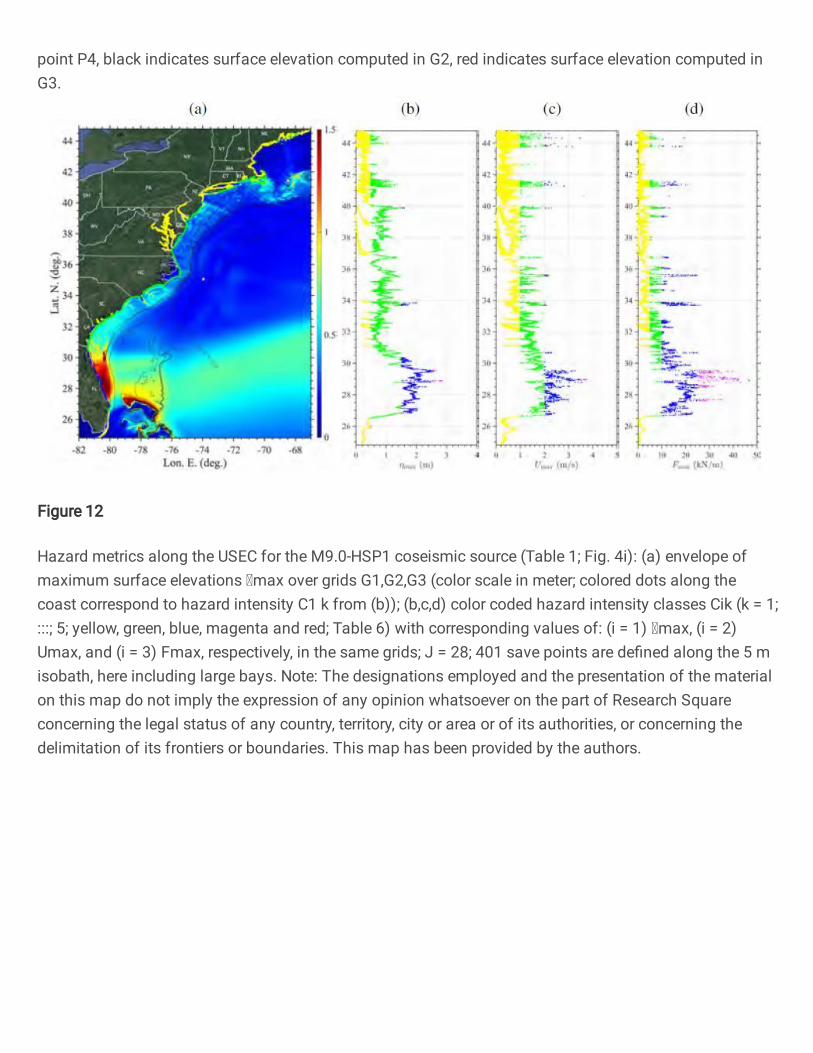
point P4, black indicates surface elevation computed in G2, red indicates surface elevation computed inG3.
Figure 12
Hazard metrics along the USEC for the M9.0-HSP1 coseismic source (Table 1; Fig. 4i): (a) envelope ofmaximum surface elevations max over grids G1,G2,G3 (color scale in meter; colored dots along thecoast correspond to hazard intensity C1 k from (b)); (b,c,d) color coded hazard intensity classes Cik (k = 1;:::; 5; yellow, green, blue, magenta and red; Table 6) with corresponding values of: (i = 1) max, (i = 2)Umax, and (i = 3) Fmax, respectively, in the same grids; J = 28; 401 save points are de�ned along the 5 misobath, here including large bays. Note: The designations employed and the presentation of the materialon this map do not imply the expression of any opinion whatsoever on the part of Research Squareconcerning the legal status of any country, territory, city or area or of its authorities, or concerning thedelimitation of its frontiers or boundaries. This map has been provided by the authors.

Figure 13
Same results as in Fig. 12, for the M9.0-PRT3 coseismic source (Table 3; Fig. 5h). Note: The designationsemployed and the presentation of the material on this map do not imply the expression of any opinionwhatsoever on the part of Research Square concerning the legal status of any country, territory, city orarea or of its authorities, or concerning the delimitation of its frontiers or boundaries. This map has beenprovided by the authors.

Figure 14
Envelope at the 5 m isobath (J = 18; 201 save points excluding large bays) of maximum tsunami: (a)elevation; (b) current; (c) momentum force; and (d) arrival time, computed in grids G1,G2,G3, for the tenACZ/LSB sources (Table 1; Fig. 4): (green) M8.0-MTR1, M8.0-MTR2; (yellow) M8.3-MTR1, M8.3- MTR2;(magenta) M8.7-MTR1, M8.7-MTR2; (red) M9.0-MTR1, M9.0-MTR2; and (black) M9.0-HSP1, M9.0-HSP2.Note, arrival times for the latter two sources, which are slightly longer, are not shown for clarity.
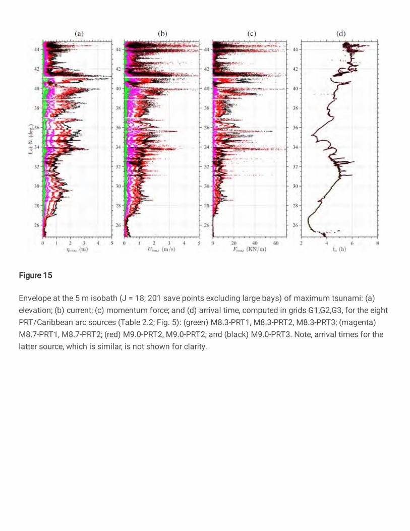
Figure 15
Envelope at the 5 m isobath (J = 18; 201 save points excluding large bays) of maximum tsunami: (a)elevation; (b) current; (c) momentum force; and (d) arrival time, computed in grids G1,G2,G3, for the eightPRT/Caribbean arc sources (Table 2.2; Fig. 5): (green) M8.3-PRT1, M8.3-PRT2, M8.3-PRT3; (magenta)M8.7-PRT1, M8.7-PRT2; (red) M9.0-PRT2, M9.0-PRT2; and (black) M9.0-PRT3. Note, arrival times for thelatter source, which is similar, is not shown for clarity.

Figure 16
Tsunami intensity index computed for ten LSB/ACZ sources (Table 1; Fig. 4), based on results of the 4hazard metrics in Fig. 14: (a,b) M8.0-MTR1; (c,d) M8.0-MTR2; (e,f) M8.3-MTR1; (g,h) M8.3-MTR2; (i,j)M8.7-MTR1; (k,l) M8.7-MTR2; (m,n) M9.0-MTR1; (o,p) M9.0-MTR2; (q,r) M9.0-HSP1; (s,t) M9.0-HSP2. TIImetric weights are wi = [0.40, 0.30, 0.15, 0.15], and color coded hazard intensity classes are: (yellow) low;(green) medium low; (blue) medium (magenta) medium high, (red) heigh, and (black) extreme. Note, for
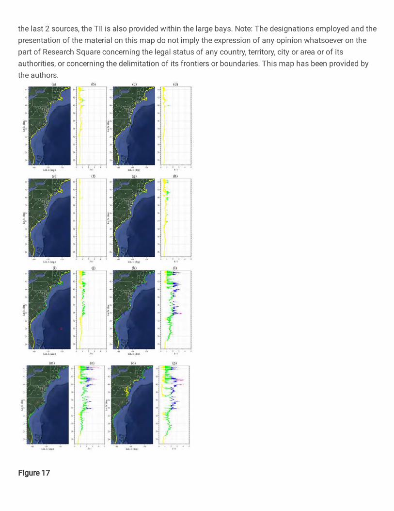
the last 2 sources, the TII is also provided within the large bays. Note: The designations employed and thepresentation of the material on this map do not imply the expression of any opinion whatsoever on thepart of Research Square concerning the legal status of any country, territory, city or area or of itsauthorities, or concerning the delimitation of its frontiers or boundaries. This map has been provided bythe authors.
Figure 17
Tsunami intensity index computed for eight PRT/Caribbean arc sources (Table 3; Fig. 5), based on resultsof the 4 hazard metrics in Fig. 15: (a,b) M8.3-PRT1; (c,d) M8.3-PRT2; (e,f) M8.3-PRT3; (g,h) M8.7- PRT1;(i,j) M8.7-PRT2; (k,l) M9.0-PRT1; (m,n) M9.0-PRT2; (o,p) M9.0-PRT3. TII metric weights are wi = [0.40, 0.30,0.15, 0.15], and color coded hazard intensity classes are: (yellow) low; (green) medium low; (blue)medium (magenta) medium high, (red) heigh, and (black) extreme. Note, for the last source, the TII is alsoprovided within the large bays. Note: The designations employed and the presentation of the material onthis map do not imply the expression of any opinion whatsoever on the part of Research Squareconcerning the legal status of any country, territory, city or area or of its authorities, or concerning thedelimitation of its frontiers or boundaries. This map has been provided by the authors.
Supplementary Files
This is a list of supplementary �les associated with this preprint. Click to download.
HSP1.mp4
PRT3.mp4