durham e-theses a critical review of currently available...
TRANSCRIPT
Durham E-Theses
A critical review of currently available pore pressure
methods and their input parameters: glaciations and
compaction of north sea sediments.
Gyllenhammar, Carl Fredrik
How to cite:
Gyllenhammar, Carl Fredrik (2003) A critical review of currently available pore pressure methods and their
input parameters: glaciations and compaction of north sea sediments., Durham theses, Durham University.Available at Durham E-Theses Online: http://etheses.dur.ac.uk/4090/
Use policy
The full-text may be used and/or reproduced, and given to third parties in any format or medium, without prior permission orcharge, for personal research or study, educational, or not-for-pro�t purposes provided that:
• a full bibliographic reference is made to the original source
• a link is made to the metadata record in Durham E-Theses
• the full-text is not changed in any way
The full-text must not be sold in any format or medium without the formal permission of the copyright holders.
Please consult the full Durham E-Theses policy for further details.

Academic Support O�ce, Durham University, University O�ce, Old Elvet, Durham DH1 3HPe-mail: [email protected] Tel: +44 0191 334 6107
http://etheses.dur.ac.uk
2
A critical review of currently available pore pressure methods and their input
parameters.
Glaciations and compaction of North Sea sediments.
A copyright of this thesis rests with the author. No quotation from it should be published without his prior written consent and information derived from it should be acknowledged.
By
Carl Fredrik Gyllenhammar
0 NOV 2003
This thesis was submitted as the fulfilment of the requirements for the degree of Doctor of Philosophy
C a r l l - redr ik G y l l e n h a m m a r i

Abstract
Historically pore pressure evaluation in exploration areas was based on empirical
relationships between drilling parameters, wireline logs and the mud weight.
Examples include Eaton's Ratio and the Hottman & Johnson Methods, which were
based on data from the Gulf o f Mexico. These methods are not readily transported to
other areas, such as the North Sea Basin, where the sediments are different in
character and where burial and temperature histories are distinctly different.
Data from several offshore North Sea wells, with high quality wireline and associated
data have been analysed to determine the most appropriate method to estimate pore
pressure in mudrocks. The data have led to an understanding o f the key parameters
for successful pore pressure estimation. The most effective method is shown to be the
Equivalent Depth Method, but only where disequilibrium compaction is the source o f
the overpressure in the mudrocks.
Core samples from 576 British Geological Survey sites in the offshore area o f the
British Islands were compared with > 10,000 porosities collected f rom the deep oceans
(DSDP/ODP sites), which show that the porosities in the shallow section in the North
Sea are anomalously low. The shallow section o f the North Sea includes large
volumes o f Pleistocene-Recent sediments deposited as glacial and inter-glacial
deposits. Frequency analysis (Cyclolog) o f the wireline data covering this interval in
several North Sea wells revealed a pattern in the relative featureless original data.
Comparison wi th the global signature for oxygen isotopes for the same time period
suggests that there have been ten cycles o f ice sheet build up (Glacial period)
followed by melting (Interglacial period) during the last one mil l ion years. Glacial
deposits from 10 individual glacial cycles have therefore been identified in several
exploration wells in the North Sea. Implications o f loading/unloading o f ice for the
migration and trapping o f hydrocarbons in the North Sea Basin are assessed.
Car l F redr ik G v i l e n h a m m a r

Acknowledgements
First I must thank my supervisor, Richard Swarbrick (Dick). I met Dick first time in
December 1995 in London. It was the first GeoPOP meeting I attended representing
Norske Conoco. When a year later I expressed interest in doing a PhD at the
university o f Durham, his enthusiasm, despite my age, made what was laying ahead
possible. M y wife Marit and I left our jobs late 1998, we sold our house in Stavanger
and moved to Durham with our two children, Elen-Martine and Fredrik.
At the university I found Dick's continues support and interest in my subject as well
as the requirement to deliver regular reports to GeoPOP an assurance for continued
progress. Neil Goulty was never far away to discuss any dif f icul t equation. Both his
and Dick's enthusiasm for my "ice theory" made this thesis what it is. I had also help
f rom Fred Wollard's long experience with using principle component analysis. The
last year in Durham I was lucky to share an office with Martin Traugott. He shared his
long experience in pore pressure prediction as well as his own developed software
PresGraf with me.
M y thanks also goes to Norske Conoco, in particularly James Middleton. They
supplied the well data I used as well as providing financial support for the project.
Thanks go to all those from GeoPOP who were there to help and exchange ideas,
Toby, Paul, Daniel, Neville, Gareth Yardley, Andy Apl in and Yunlai Yang.
Finally many thanks to my new colleges at BP, for their support during the last year,
Nigel Last, Mark Alberty and Mike McLean.
C a l l Freclrik G y l i e n h a m r n u r iii
Table of Contents
Abstract i i Acknowledgements i i i Table of Contents iv List of Tables vi List of Figures v i i Declaration xi Chapter 1 Introduction 1
1.1 Background 2 1.2 Data 3 1.3 Introduction 7 1.4 Pressure, the basic concepts 11 1.5 Aims and layout of thesis 14
Chapter 2 Pore Pressure Evaluation Concepts and definitions 16 2.1 Definition 17
2.1.1 Mudrock porosity 18 2.1.2 Different porosity evaluation equations 18 2.1.3 Normal compaction curve and trend lines 23
2.1.3.1 Athy-type re lationship 24 2.1.3.2 Soil mechanics relationship 25 2.1.3.3 Athy - Soil mechanics: how are they different 25
2.1.4 Vertical versus mean effective stress 28 2.2 Pore Pressure Calculation Methods 29
2.2.1 Vertical Methods 30 2.2.1.1 Equivalent depth method 30 2.2.1.2 Harrold method 32 2.2.1.3 Explicit method using the resistivity log 33
2.2.2 Horizontal methods 35 2.2.2.1 Eaton Method 35 2.2.2.2 The pore pressure calculation program; PresGraf 37
2.2.2.2.1 PresGraf normal compaction trend 37 2.2.3 Seismic 40 2.2.4 ShaleQuant 41 2.2.5 Principle Component Analysis 41
2.3 Drilling parameters 46 2.3.1 Real time data 48 2.3.2 D'exponent 48 2.3.3 Torque 54 2.3.4 Hydraulics 55 2.3.5 Bit type and wear 55 2.3.6 Lagged data 56
2.3.6.1 Gas 56 2.3.6.2 Cuttings and Cavings 58 2.3.6.3 Mud temperature in and out 58 2.3.6.4 Mud resistivity in and out 58
2.3.7 Mud chemistry and mud-formation chemical reactions 59 Chapter 3 Comparison of different pore pressure methods using a North Sea well 60
3.1 Introduction 61 3.2 Pore pressure evaluation of well 1/6-7 in the North Sea, Norwegian sector 61
3.2.1 Pore pressure evaluation while drilling (wellsite) 62 3.2.2 The Post-well analysis • 63
3.2.2.1 Tertiary 67 3.2.2.2 Chalk 67
Car l F redr ik G v H e n h a i n m a r iv

3.2.2.3 Jurassic 67 3.3 Normal Compaction in the North Sea 69
3.3.1 Palaeocene and Lower Eocene 75 3.3.2 Normal compaction from resistivity data 76
3.4 Wireline log pore pressure calculation 78 3.5 Comparing the North Sea with the Gulf of Mexico Basin 86 3.6 Vimto#land#2 88 3.7 Summary and conclusions 93
Chapter 4 The impact of the Glaciation on the Normal compaction in the North Sea 96 4.1 Introduction 97 4.2 Glacial history 99
4.2.1 The Neogene - Pleistogene sedimentary succession 102 4.3 Tills 103 4.4 Mudrock porosities 104 4.5 Oxygen isotope data 106 4.6 Time series frequency analysis (CycloLog) 108 4.7 Ice loading and pore pressure 112 4.8 Subglacial water flow .....118
4.8.1 Resistivity log response 121 4.9 Hydrocarbon migration 122 4.10 Erosion of the Scandinavia during Quaternary 123 4.11 Conclusions 124
References: 126 Appendix 1 136 Appendix 2 145 Appendix 3 155
C a r l F i e d n k G v l l e n l i a m m a ! ' v

List of Tables
Table 2-1 Eigenanalysis o f the correlation matrix 42 Table 2-2 A list o f measurements that can be used to interpret the shale pore pressure.
47 Table 2-3 Eigenanalysis o f the correlation matrix 52 Table 4-1 BGS sits and exploration wells 105 Table 4-2 The f low rates are calculated assuming hydrostatic pressure in the aquifer
underlying the aquitard 120
Cur l l-reclrik G y l l e n h a m m a r vi
List of Figures
Figure 1.1 The wireline log plot of well 1/6-7 f rom seabed to 2000m 4 Figure 1.2 The wireline log plot o f wel l 1/6-7 f rom 1900 to 4000m 5 Figure 1.3 The wireline log plot o f well 1/6-7 f rom 3000 m to 4995 m (TD) 6 Figure 1.4 Schematic of wireline logging. The lithological column to the right is a
schematic o f a pressure probe (RFT) being used to measure the pore pressure in permeable sandstone 9
Figure 1.5 Pressure plotted against depth in a fictional well. The effective stress is equal to the overburden pressure minus the pore pressure and the overpressure is equal to the pore pressure minus the hydrostatic pressure 12
Figure 1.6 The Figure to the right shows how a pressure versus depth plot (left, Figure 1.5) becomes presented as pressure gradient versus depth 14
Figure 2.1 a,b,c,d. l a porosity variation as a function o f sonic velocity. B, porosity versus bulk density. C, the sensitivity to pore water density. D, the sensitivity to matrix density 20
Figure 2.2 Log derived porosities in well Nor-1/6-7 Norway. The low porosity interval f rom 3261m to 4346m depth is the Cretaceous Chalk. The values are listed in Appendix 1 23
Figure 2.3 Comparison o f porosity wi th effective stress for the Athy and the SM equations. Initial porosity (sea floor porosity) for Athy is 0.7 (70 % ) while the porosity at 100 kPa (approximately 100 meters below sea floor) is 0.66 (66 % ) The compaction factors a re for Athy; 0.00008 and SM; 0.74 26
Figure 2.4 The relation ship between porosity, solidity and void ratio is shown. The y-axis is the compaction as a length reduction. It is assumed that a confined volume is compressed beginning with a void ratio o f four 27
Figure 2.5. Porosity from a pseudo well is plotted versus depth. Integrating the density log and subtracting the hydrostatic pressure calculate the effective stress. The two normal compaction curves are coming from Figure 2.3 30
Figure 2.6 Porosity f rom a pseudo well is plotted versus mean effective stress. The two normal compaction curves are coming f rom Figure 2.3. See text for an explanation for the equivalent effective stress method 32
Figure 2.7 Comparing the porosity derived f rom the sonic, density and neutron log with the resistivity derived using the equation 1.37 proposed by Alixant and Desbrandes(1991) 34
Figure 2.8 The PresGraf normal compaction trend to the left compared with the Athy normal compaction curve (Figure 2.3) to the right 39
Figure 2.9 Scree plot o f the eigenvalue o f each principal component o f the PCA of the wireline logs 43
Figure 2.10 a, b, c and d. The plots to the left (a and c) are cross sections through data perpendicular to PCI , PC2 and PC3. b and d show the loading values with respect to the different principal components 44
Figure 2.11 a and b. PCI versus depth in blue and the sonic travel time in green 46 Figure 2.12 The plot shows the d'exponent and the corrected d'exponent versus depth.
The straight lines are trend lines representing one particular pressure gradient (one mud weight) 49
Figure 2.13 Cross plot o f the d'exponent versus the sonic travel time, well N 1/6-7. It suggests a good relationship between the sonic log and the d'exponent in the Tertiary section (pink squares). The correlation is less obvious in the Jurassic (yellow triangles). There is no correlation in the Chalk 50
C a r l Frecii ik G v l l e n h a m m a r vn

Figure 2.14 Cross plot of the d'exponent versus the resistivity log. The plot show no correlation 51
Figure 2.15 Scree plot of the eigenvalue of each principal component of the PCA of the drilling parameters 53
Figure 2.16 a, b, c, d. The plots to the left (a and c) are cross sections through data perpendicular to PCI, PC2 and PC3. b and d show the loading values with respect to the different principal components 53
Figure 2.17 a, b and c. PCI versus depth with the standardized log porosity overlaid in Figure b and the normalized sonic travel time in Figure c 54
Figure 3.1 The corrected d'exponent plotted versus depth with a normal trend line overlaid in green. Normally new trend lines will be added paralleling the green line each time a new bit is put on the drill string. The new line will represent the actual MW. An alternative trend line is suggested in red. That trend line will also result in a reasonable calculated pore pressure at the target of interest (i.e. 4200 to 4800 m) 63
Figure 3.2 The sonic velocities in the shale sections plotted against depth on a semilogaritmic graph. The yellow line is the best visual fit trend line 65
Figure 3.3 A comparison of the calculated pore pressure from the d'exponent (blue dots) and the sonic velocity calculated pore pressure 66
Figure 3.4 Shale velocities from the wells in Figure 3.2 compared with the wells used by Hansen (1996). The Figure to the left has a logarithmic X-axis. At such a plot the Athy type normal compaction trend become a straight line. On the plot to the right it is much more obvious that the well used in this study are different from the one used by Hansen (1996) 70
Figure 3.5 Porosity data from 10000 DSDP/ODP mudrock samples. ODP site #336 is in the deep water Norwegian Sea. The yellow curve is the suggested normal compaction trend drawn through the data set 71
Figure 3.6 Compaction trends as plotted as void ratio versus effective stress. Al l the different trends that have been tested in this chapter are overlaid. The PresGraf (in blue) is an approximation as the real curve is proprietary data to BP 72
Figure 3.7. Different wireline methods to calculate the volume of clay are compared in well N 1/6-7. The red dot are Vcl form using the GR log, the blue dots from the neural network (ShaleQuant and the green dots the neutron and density log.
74 Figure 3.8 Twenty-six wells in 5 offshore areas and 4 onshore fields (MacGregor,
1965). The pink line is a suggested normal trend for the Gulf of Mexico 77 Figure 3.9 Pore pressure in mega-Pascal versus depth in meters. The green solid line
is the overburden and the blue solid line is the hydrostatic pressure. The equivalent depth method calculated pressure is in blue dots while the orange is the University of Durham method. The dashed black curve is the operator's interpretation while the olive solid line is the mud weight. The red crosses are the RFT direct pore pressure measurements 79
Figure 3.10 Pore pressure in mega-Pascal versus depth in meters. The green solid line is the overburden and the blue solid line is the hydrostatic pressure. The Eaton equation with the sonic log as input (red dots) compared with the Equivalent depth method with the porosity as input (blue dots). The red crosses are the RFT direct pore pressure measurements. The values are listed in Appendix 2 82
Figure 3.11 Pore pressure in mega-Pascal versus depth in meters. The green solid line is the overburden and the blue solid line is the hydrostatic pressure. The Eaton equation in red dots compared with the Equivalent depth method in solid blue,
Cur l Fredr ik G v i l e n h u f f i m ; i r V l l l

both with the sonic log as input. The red crosses are the RFT direct pore pressure measurements. The values are listed in Appendix 2 83
Figure 3.12 Pore pressure in mega-Pascal versus depth in meters. The green solid line is the overburden and the blue solid line is the hydrostatic pressure. The Equivalent depth method tested with two different normal trends. The Athy equation used by the operator o f well Nor-1/6-7 (blue dots) versus the DSDP-ODP based trend (red dots).The red crosses are the RFT direct pore pressure measurements. The values are listed in Appendix 2 83
Figure 3.13 The shale porosity (red solid curve to the right) and the shale travel time (green solid line to the right) versus depth in the Jurassic section. The x axis is in % for porosity, u,sec/ft for the sonic log. The curves to the left o f the overburden (strait solid green line) is in MPa. Between the overburden and the hydrostatic pressure (left most solid blue) are from left the pore pressure calculated using the sonic log as input (blue curve) then with porosity as input (orange curve). The values are listed in Appendix 2 84
Figure 3.14 Figure 3.13, the pressure transition zone f rom 4850- 4890 meters. The values are listed in Appendix 2 84
Figure 3.15 Pore pressure in mega-Pascal versus depth in meters. The green solid line is the overburden and the blue solid line is the hydrostatic pressure. The Eaton equation with the resistivity log as input (green dots) compared with the Eaton sonic (red dots). The red crosses are the RFT direct pore pressure measurements. The values are listed in Appendix 2 85
Figure 3.16 Depiction o f salt features in the area around the basin. The local depocenteres are termed mini-basins (Yardley and Couples, 2000) 87
Figure 3.17 Comparison o f the NRG derived shale porosity versus permeability curves, wi th some basin modelling default curves. A range o f clay-fractions are shown, f rom 20% to 80% (Yang and Apl in , 2000) 89
Figure 3.18 Comparison o f the GeoPOP derived shale compaction curves with some basin modelling default curves. A range o f clay fractions are shown, f rom 20% to 80% (Yang and Apl in , 1999) 90
Figure 3.19 Pore pressure prediction for Vimto #2. The blue curve is the pore pressure calculated using the Eaton method and the shale sonic velocity as input. The red line is pore pressure using the equivalent depth method. The pink diamonds are the M D T pressure points. The red line to the left is the overburden. The values are listed in Appendix 3 91
Figure 3.20 The reservoir section for well Vimto#2. The M D T pressures are generally 50 to 100 psi higher than the calculated shale pressures 91
Figure 3.21 The red curve is the pore pressure calculated f rom a 2-D model alowing for lateral transfere (Yardley and Couples, 2000) 92
Figure 4.1 A curve showing the variation in oxygen isotope composition o f the sea-water for the last 6 mil l ion years. The oxygen isotope data are based on foraminifera f rom three boreholes near the coast o f Ecuador (Shackleton et al., 1990; Shackleton et al., 1995 98
Figure 4.2 Reconstruction o f the Scandinavian and British Ice Sheet during a glacial stadial (after Hughes, 1998). The maximum ice thickness onshore was 2600 m and the maximum thickness in the offshore North Sea was approximately 1600 m 101
Figure 4.3 Porosity versus depth. A compilation o f core measurements and wireline calculated porosities 106
Car l I - re l ink G v l l e n h a m m a r I X

Figure 4.4 To the left is the oxygen isotope data shown in Figure 4.1. To the right is the GR log followed by the filtered GR log f rom well Nor-1/3-2. The third curve is picks representing sudden changes in the cyclicity o f the filtered GR curve. The third curve show peaks, positive or negative representing sudden transitions from high to low GR value, shown as a negative peak (to the left). The opposite results in a positive peak. The last curve is the integration o f previous curve. These curve were output f rom CYCLOLOG*. This curve represents the cumulative difference between the predicted log values and the actual log values. Breaks in the cyclicity succession may be related to missing sections or abrupt changes in sedimentation rates. A large positive peak could be a condensed section 109
Figure 4.5 Correlation o f five wells drilled in the southern part o f the Norwegian sector using CycloLog software. The distance f rom Nor-1/3-2 to Nor-2/11-7 is about 100 km (60 mils). The cycles are compared on the left with oxygen isotope signature (See text) 111
Figure 4.6 The four maps above present the palaeo-coastline for each subsequent crustal motion model. It is important to note that large parts o f the North Sea were dry land after the last deglaciation, in each case for a period o f several 1000 years 113
Figure 4.7 The figure to the left show a typical pore pressure profile in the North Sea with no seawater just prior to a glaciation. The sand at 2000 meters subcrope to seafloor and has therefore hydrostatic pressure. During glaciation o f the North Sea the overburden pressure and the hydrostatic pressure increase with a pressure equivalent to the weight o f the ice-sheet. I f the sand subcrops under the ice-sheet the pore pressure w i l l also increase in the sand. But i f i t subcrops outside the ice-sheet, its pore pressure w i l l only vary as much as the sealevel changes 114
Figure 4.8 The profile B-B' shown on Figure 4.7. It show that the maximum subsidence was in the centre o f the Baltic Sea o f more than 400 metres, while it was potentially uplif t in the North Sea (Milne et al., 1999, Mitrovica et al., 1994, Tushingham, A . M . , 1991) 116
Figure 4.9 Resistivity curves f rom the North Sea compared with Gul f o f Mexico. The graph to the left is raw data while the raw resistivity curves have been temperature corrected on the graph to the right 122
Carl Fredrik Gyllenhammar x

Declaration
The content o f this thesis is the original work o f the author (other people's work, where included, is acknowledged by reference). It has not been previously submitted for a degree at this or any other university.
Carl Fredrik Gyllenhammar Durham September 2003
Copyright
The copyright o f this thesis rests wi th the author. No quotation f rom it should be published without his prior written consent and information derived f rom it should be acknowledged.
Cur! F redr ik G y l l c n h a m m a r xi

Chapter 1 Introduction
C a r l F redr ik G v i l e n h u m m u r 1
h i ! i - o ; H k ' ; i o n
1.1 Background
Fifteen years ago, most pore pressure studies were undertaken solely for safety
aspects in the design and drilling o f exploration wells. As the need for accurate pore
pressure evaluation is growing due to its general application in exploration studies
such as hydrocarbon migration studies, more accurate methods founded on sound
physical principles, and not just empirical observations, are needed.
Pore pressure estimation is a particular challenge in the North Sea on account o f the
complex tectonic and sedimentological history o f the region, where the highest
overpressure (pore pressures above the normal, hydrostatic pressure) are found in
Jurassic and Triassic reservoir sandstones. The presence o f a thick Chalk section as
well as a variety o f mudrock types, including a kerogen-rich petroleum source rock,
challenge standard practices for pore pressure evaluation which were, in many cases,
developed in the Gulf o f Mexico where the rocks are younger and exclusively
siliciclastic (sandstone, siltstones and shale mudrocks). The late history (Pleistocene-
Holocene) o f the North Sea has involved ice loading and the deposition o f glacially-
derived sediments which add a further component o f complexity to the stress and
f lu id history o f North Sea sediments.
The availability o f a very high quality set o f well data f rom the Norwegian North Sea
(Central Graben) provided impetus for this project which was designed to test current
methods o f pore pressure prediction, assess the impact o f a late ice-loading and
unloading history and apply new technology on mudrock compaction (being
concurrently developed in the GeoPOP research group - see below).
There are a number o f complementary data which can be used for pore pressure
evaluation including basin modelling, seismic velocities, wireline logs and drilling
parameters. Each requires different data input and interpretation requirements. In this
thesis the emphasis is for pore pressure evaluation using wireline logs. The response
f rom the drilling parameters was used as an independent control.
C a r l 1-reilrik G y l l e n h a m m a r 2

Chapter I I n i r ouu i ' i ion
The thesis was funded by Norske Conoco in Norway and the work was included as part o f GeoPoP. GeoPoP (GEOsciences Project into OverPressure) was a joint research project involving University o f Durham, Newcastle University, Heriot Watt University and industrial sponsors such as major oi l companies like BP, Amoco, Statoil, Norsk Hydro, Phillips, Conoco, etc. The aim o f GeoPOP was to explain how pore pressures evolve in mudrocks and to evaluate and develop new methods to predict and calculate the pore pressure in these sediments.
1.2 Data
Norske Conoco made most o f the data available, consisting o f wireline data f rom
exploration wells. The most important well was 1/6-7, drilled by Norske Conoco in
1989, which is classified as a high pressure (> 10,000 psi) and high temperature
(>350°F) (HPHT) well . In addition to well 1/6-7 were a number o f offset wells in the
southern part o f the Norwegian shelf. The data set included also some wells f rom
Haltenbanken and the Barents sea. Well 1/6-7 has high quality wireline and mud
logging data particularly with respect to testing pore pressure prediction and
calculation methods (Figure 1.1, 1.2 and 1.3).
GeoPOP provided the data f rom the Gulf o f Mexico. Data f rom the shallow coring
project by British Geological Survey (BGS) were provided by BGS. Data f rom the
Ocean Dri l l ing Project (ODP) are freely available on the Internet and were
downloaded free o f any charge.
Frednk G v l k ' n l u u n m a r

Chapte r I I n t r u d m / i i u n
WELL N1 6-7 Q —
I r | i | I " V T C X A T L r_j
0 . C U t L M L L E T L
71 i H L I B L I T L T ZL <X L L S A J T — T M t J O
I L 1. t1
i r 1 L_l I :- L r.
• • - n F"W4J I K »* *
-4DD J E : -If fa •
i •
LDD
L J
S f f
• Lt r• [•
l.L [•[•
. 7(,r,
, - r . t . !
H O ['
L.M-f
:
L L C C
Li ft-
I i l l
. 1 M
Figure 1.1 The wireline log plot of well 1/6-7 from seabed to 2000m.
Carl Fredrik Gyllenhammar 4
Chapter
I t tw
U N
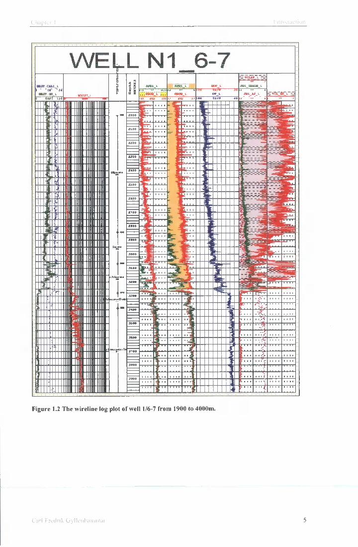
Figure 1.2 The wireline log plot of well 1/6-7 from 1900 to 4000m.
Carl Fredrik Gyllenhammur 5

W E L L N1 6-7 «£T CALL L
I I M I I U I I > I I I UK liiilli ill III! -1111111 I I I iir-iunir mil llE?i!MIII|i i l l M I I M i l l l l 'II I I I K I I I I I H I M i m i i i i i i u i i ISM iiiiiiiiniii iimiimiii lllllllllllll L illllllllllll E m i n i u m ?
H I I I S H I I I I I fiiihiinii ii HIIBIIIII llli lllllllllllll I I I N I I U I I I I I I I I I I [ I I I E I I I I I I I I I I I HIIE2IIIIII I I I
I I I I M I I I I I I I I I I I E I I I I I I I I I I I
I W I B I I I I H I I I [ I I M I I I I I I I IF ' . n u l l u m r: L U K I I I I I I I I I ;i I 'DlgHUM 111:' It iSillllll -I I M - . " i l l l I ' E i ^ i i l l l l ICSUUII I I : llllli Ull' Illril l l lSi lit. Will
I I I I n u n mi win I ' ^ l l l l l I M I I I I I I I l.»?llllll.
IHICtMi iTM
"mi IIIIII IIIIII I i i i iJi l l l! IIIIII E siiiiimiiimiiii 211 in i n i IIIIII IIIIII mill 1 mm mm mini IIIIII IIIIII IIIIII B IIIIII IIIIII mini IIIIII IIIIII IIIIII i i n IIIIII mini IIIIII IIIIII mini
T *
3§ or l rai sum l
immmFh
Figure 1.3 The wireline log plot of well 1/6-7 from 3000 m to 4995 m (TD).
( ai l Fredrik Gvl lenhumniur 6
1.3 Introduction
In exploration dril l ing operations pressure f rom the circulating dril l ing f lu id (mud) is
used to prevent the pore f lu id in the porous rock entering the borehole. The pressure
from the mud at a particular depth is a function o f the average density ( M W = Mud
Weight) and the vertical height o f the column f rom that depth to the surface. In low
permeability formations, such as mudrocks, the formation can cave into the wellbore
through tensile failure i f the pore pressure is higher than the counter pressure from the
mud. The industry has a long history o f establishing empirical relationships between
drilling parameters such as the rate o f penetration and the gas measured in the
returning dril l ing f lu id to the pore pressure in the mudrocks. The uses o f dril l ing
parameters are very subjective and prone to large uncertainties. The pressure can also
be calculated indirectly f rom petrophysical measurements. Petrophysical data can be
acquired while dri l l ing or after dril l ing a section. In the former case the petrophysical
sensors are placed behind the dri l l bit in operations known as Logging While Dri l l ing
(LWD) or Measurement While Dri l l ing ( M W D ) . When data is acquired once drilling
has been completed, the petrophysical sensors are lowered down the hole suspended
f rom a wire (wireline logging) and readings taken by the tools while being reeled back
up. The pore pressures in the reservoir rocks with high permeability are measured
directly using a wireline tool wi th a pressure gauge. A cylindrical probe with a small
aperture is hydraulically forced into the formation (Figure 1.4) and the tool remains at
the location until the pressure stabilizes between the inside o f the tool (where the
pressure gauge is located) and the formation (where the probe has been extended).
The pressure is recorded as pressure vs time. The most common trade acronyms for
these tools are RFT (Repeat Formation), FMT (Formation multi-tester) or M D T
(Modular Dynamics Tester). In mudrocks where permeability is very low, this tool
cannot be used due to the time it w i l l take for pressure to stabilize. Direct pressure
measurements are also recorded when a hydrocarbon zone is tested, called a Dr i l l
Stem Test (DST).
The accompanying petrophysical measurements collected at the same time as the
pressure tests include sonic, velocity, neutron porosity, density, and resistivity (unless
you intended to list something else). These sensors are all calibrated for the porous
formation and w i l l tend to give erroneous reading i f any clay minerals are present.
C'ai! h e d n k G v i l e n l n u r i i n a i ' 7
Inli'oduciion
The challenge is therefore to use these measurements in mudrocks wi th low
permeability and high clay content. During compaction o f compressible sediment,
such as mudrock, water is expelled and the porosity decreases. I f the free water which
needs to be expelled to maintain equilibrium with the imposed stresses cannot drain
out o f the system, the porosity w i l l not decrease, wi th the result that the pore pressure
increases above the hydrostatic pressure. Porosity cannot be measured directly in a
borehole. The porosity is calculated indirectly f rom the sonic velocity, neutron
porosity, density or the resistivity measurement, or a combination o f these
measurements. The effective or inter-granular stress is then calculated using a
relationship between the porosity, the normal compaction trend and the total
lithostatic stress (overburden stress).
A variety o f empirical relationships have been developed for calculating mudrock
porosity f rom different log responses. Typically, a stress-porosity relationship is not
used directly, but instead porosity is compared against a normal compaction trend,
which would be the porosity against depth for the location in question assuming a
'normal' pressure profile equivalent to the hydrostatic head of a water column. In this
work it w i l l be shown that the normal compaction trend often yields the biggest
uncertainties in calculating the pore pressure in mudrocks.
Carl Fredr ik G y 1 lenhann 1 i;ii 8

Figure 1.4 Schematic of wireline logging. The lithological column to the right is a schematic of a pressure probe (RFT) being used to measure the pore pressure in permeable sandstone.
Having inferred mudrock porosity f rom logs and computed or established a normal
compaction trend o f expected porosity for normal pressure, the final step is to f ind a
relationship quantifies the pore pressure magnitude associated with a mismatch
between the estimated mudrock porosity f rom log response and the normal
compaction trend.. This transform or equation might be based on physical principles,
such as the equivalent depth (or effective stress) method, or empirical relationships,
such as the Eaton's method. It w i l l be shown that the transform method used for
calculating the pore pressure is less important than the choice o f normal compaction
trend.
Carl Fredrik Gyllenhammar 9

Chapter i
The initial goal for this research was to establish a new method to calculate the pore
pressure in mudrocks as a function o f petrophysical measurements. During the course
of this research it became apparent that the classical equivalent depth method is a
reliable equation and it would be o f limited value to attempt an improvement to it.
Also, the porosity o f the mudrocks can be reliably calculated f rom a combination o f
the available wireline logs. A sensitivity study shows clearly that the biggest
uncertainty is the normal compaction curve. Eaton (1975) summarized it best: "The
methods used to establish normal trends vary as much as the number o f people who
do i t" .
A normal compaction curve represents the reference trend describing the compaction
behaviour o f sediments which are normally pressured. The compaction (porosity loss
involving expulsion o f fluids) is caused by increases in vertical and /or horizontal
stress. Conventional pore pressure prediction uses the normal compaction curve to
estimate the magnitude o f overpressure. Data f rom which normal compaction curves
are derived include shallow buried sediments o f the same age and lithology, or
published compaction relationships. For example, Hansen (1996) examined three
wells in the North Sea where he assumed that the mudrocks have normal pore
pressure. He established a relationship between the sonic travel time and the mudrock
porosity used in this research. Other approaches are based on laboratory
measurements o f compaction such as by Skempton (1970) where he showed a
relationship between compaction and the volume of fine-grained material in the
samples. The shortcoming o f that approach is that the relationship does not take into
account the different compaction behaviours o f clay minerals such as montmorillonite
versus fine-grained quartz, (K. Bjorlykke (2001) personal oral cornmun.).
This research shows that it is unlikely that any useful normal compaction trend can be
established in the North Sea due to recent glacial events. The glacial tills left by a
earlier glacial event have been overlooked for many years. The nature o f these
sediments is found to be very different from normal marine and non-marine shale
mudrocks. This suggest that the previous method of establishing a normal trend by
overlaying a number o f porosity curves form offset wells w i l l give wrong results i f
used in basins such as the North Sea.
Car l Frednk Gyl l cn l iammar 10
imro i iua i i jn
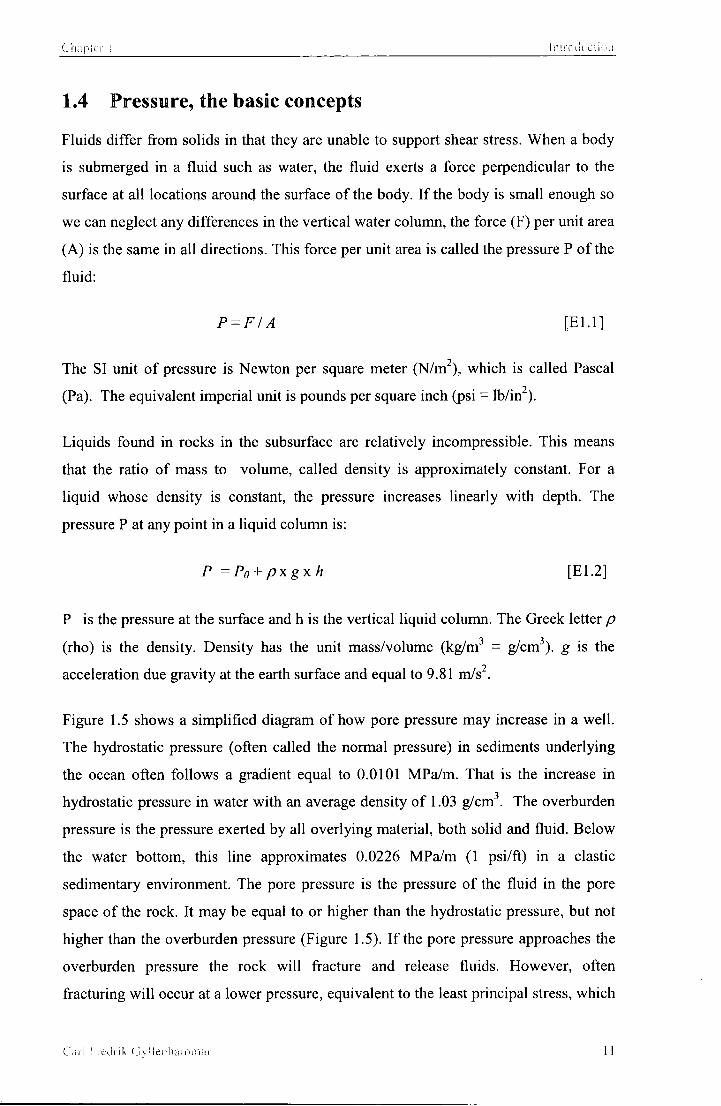
1.4 Pressure, the basic concepts
Fluids differ from solids in that they are unable to support shear stress. When a body
is submerged in a f lu id such as water, the f lu id exerts a force perpendicular to the
surface at all locations around the surface o f the body. I f the body is small enough so
we can neglect any differences in the vertical water column, the force (F) per unit area
(A) is the same in all directions. This force per unit area is called the pressure P o f the
f lu id :
P = F/A [ E l . l ]
The SI unit o f pressure is Newton per square meter (N/m 2 ) , which is called Pascal
(Pa). The equivalent imperial unit is pounds per square inch (psi = lb/in ).
Liquids found in rocks in the subsurface are relatively incompressible. This means
that the ratio o f mass to volume, called density is approximately constant. For a
liquid whose density is constant, the pressure increases linearly wi th depth. The
pressure P at any point in a liquid column is:
P =P0 + pxgxh [E1.2]
P is the pressure at the surface and h is the vertical liquid column. The Greek letter p
(rho) is the density. Density has the unit mass/volume (kg/m 3 = g/cm 3). g is the
acceleration due gravity at the earth surface and equal to 9.81 m/s 2.
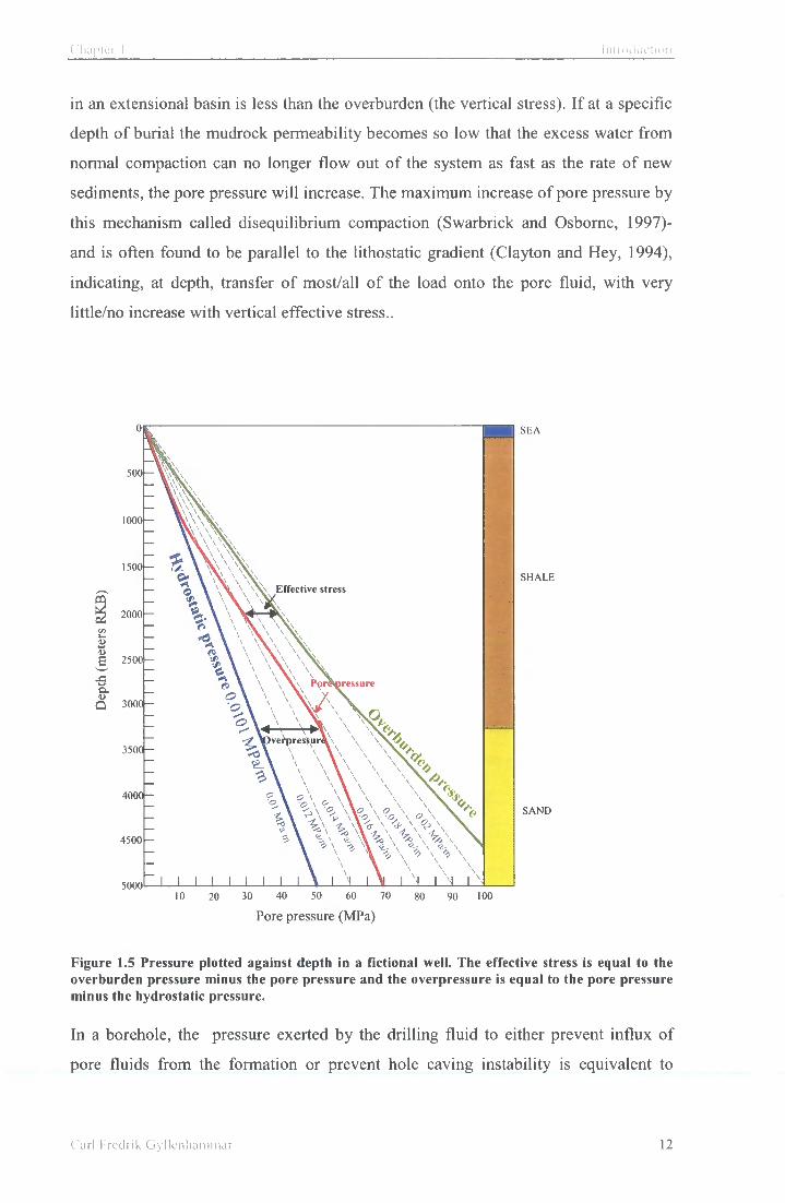
Figure 1.5 shows a simplified diagram o f how pore pressure may increase in a well .
The hydrostatic pressure (often called the normal pressure) in sediments underlying
the ocean often follows a gradient equal to 0.0101 MPa/m. That is the increase in
hydrostatic pressure in water wi th an average density o f 1.03 g/cm 3. The overburden
pressure is the pressure exerted by all overlying material, both solid and f lu id . Below
the water bottom, this line approximates 0.0226 MPa/m (1 psi/ft) in a clastic
sedimentary environment. The pore pressure is the pressure o f the f lu id in the pore
space of the rock. It may be equal to or higher than the hydrostatic pressure, but not
higher than the overburden pressure (Figure 1.5). I f the pore pressure approaches the
overburden pressure the rock w i l l fracture and release fluids. However, often
fracturing w i l l occur at a lower pressure, equivalent to the least principal stress, which
C a r l r ied i ik (Jyl lenhammiir 11
Chapter I Introduction
in an extensional basin is less than the overburden (the vertical stress). I f at a specific
depth o f burial the mudrock permeability becomes so low that the excess water f rom
normal compaction can no longer f low out o f the system as fast as the rate o f new
sediments, the pore pressure w i l l increase. The maximum increase o f pore pressure by
this mechanism called disequilibrium compaction (Swarbrick and Osborne, 1997)-
and is often found to be parallel to the lithostatic gradient (Clayton and Hey, 1994),
indicating, at depth, transfer o f most/all o f the load onto the pore f luid, with very
little/no increase with vertical effective stress..
SEA
sun
nidi)
1500 SHALE
s \
\
4J \ g 2500-
ressure r.
Q 3000 - -
•
• 3500- \
\
/J 4000-
SAND 3>\ ^ \
4500
I I I I I I 5000 70 -lo ill id 100 2U Ml 90
Pore pressure (MPa)
Figure 1.5 Pressure plotted against depth in a fictional well. The effective stress is equal to the overburden pressure minus the pore pressure and the overpressure is equal to the pore pressure minus the hydrostatic pressure.
In a borehole, the pressure exerted by the drilling f lu id to either prevent inf lux o f
pore fluids f rom the formation or prevent hole caving instability is equivalent to
C a r l Fredrik G y l l e n h a m m a r I 2

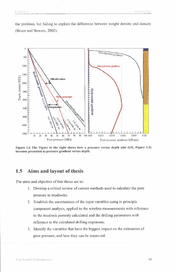
density o f the drilling f lu id and its column height. Therefore, the formation pore
pressures are often converted into dril l ing f lu id density equivalents so it is clear as
what drilling f luid density just balances the pore pressures. Figure 1.6 shows how a
typical pore pressure profile can be displayed as pressure gradient versus depth. I f one
follows the change in the pressure gradient o f the pore pressure (red curve), every
point on the curve represents a pressure gradient and a corresponding average f lu id
density that particular pressure at that depth represents. The maximum pore pressure
gradient is reached at the top o f the reservoir (3200 meters) equal 0.016 MPa/m. That
is equivalent to the pressure at the bottom of a 3200-meter vertical f lu id column with
an average f lu id density o f 1.64 g/cm 3. In exploration drilling a dril l ing mud is used
where materials such as barite is mixed to form a liquid (called dril l ing mud) wi th
such high average density. The terminology used is equivalent mud weight (EqMW).
The pressure gradient plot illustrates a big challenge while drilling these wells. The
EqMW has to be high enough to hold back the f lu id f rom the depth where the
formation has the highest-pressure gradient. However, in some formations, typically
the shallower ones, this mud density would apply a pressure significantly greater than
the pore pressures in these formations. This excess pressure may lead to fracturing o f
the rock and losses o f the drilling f lu id .
A confusing aspect in the o i l industry with regard to pressure terminology is the
mixing the terms; pressure gradient and density (EqMW). This becomes particularly
diff icul t and confusing when working with a mixture o f both imperial and the SI
units. It has already been shown that the pressure gradient equals density multiplied
by the acceleration due to gravity. In the imperial system, the norm is to use weight
density rather than density. Weight density is defined as the ratio o f the weight o f an
object to its volume. The units are pounds per gallon (ppg). As the weight is equal to
the mass multiplied with gravity, both weight density and pressure gradient have the
same units. The imperial unit system has historically been the norm in the oi l industry
and the people involved has become used to converting directly f rom weight density
(ppg) to pressure gradient (psi/ft) and to pressure (psi). The word weight density is
often shortened to density. This has created a problem when converting to the SI
system. Too often, while converting f rom density (g/cm 3) to pressure gradient
(MPa/m), density is not multiplied by gravity (9.81 m/s 2). A typical example is a
recent paper titled "Pore Pressure terminology" in the Leading Edge written to explain
C'ari I redrik G y l l e n h a m m a r 13
Chapter i Introduction
the problem, but failing to explain the difference between weight density and density
(Bruce and Bowers, 2002).
ijrn Pore prrnurr gnoient
Effective stress
I. O 3000
ft
4500
I—I- J I I I I I I I I I I I L-LJ 5000 n j ; 0.014 0.016 60 70 80 90 100 0.01 0.012 ill 20 30 .i. 50
Pore pressure (MPa) Pore pressure gradient (MPa/m)
Figure 1.6 The Figure to the right shows how a pressure versus depth plot (left, Figure 1.5) becomes presented as pressure gradient versus depth.
1.5 Aims and layout of thesis
The aims and objective o f this thesis are to:
1. Develop a critical review o f current methods used to calculate the pore
pressure in mudrocks.
2. Establish the uncertainties o f the input variables using in principle
component analysis, applied to the wireline measurements with reference
to the mudrock porosity calculated and the drilling parameters wi th
reference to the calculated dril l ing exponents.
3. Identify the variables that have the biggest impact on the estimation o f
pore pressure, and how they can be improved.
C a r l Fredrik G y l l e n h a m m a r 14

Chapter 1 I n i r o d u c t i o n
4. Compare the wireline signature o f overpressured shales in the North Sea
basin wi th those f rom the Gul f o f Mexico.
5. Examine why the resistivity measurements o f the mudrocks can be used as
input parameter to calculate pore pressure in the Gul f o f Mexico, while
this has proved diff icul t to apply in the estimation o f pore pressure in the
North Sea.
Following the introduction comes Chapter 2 where the pressure concepts with
respects to pore pressure in shallow sediments are discussed. That is followed by a
discussion o f mudrock porosity and normal compaction in mudrocks. Then the
different pressure calculation methods, first wi th wireline logs as input, then those
using drilling parameters.
Chapter 3 discusses the results f rom using these different pore pressure estimation
methods on a test well , Nor 1/6-7 in the North Sea. The sensitivity o f the input
parameters are discussed. The results f rom the North Sea are then compared with the
mudrocks f rom a mini-basin in the Gulf o f Mexico,
Chapter 4 examines the glacial history o f the North Sea to explain the nature o f the
shallow sediments, and their physical and petrophysical properties. Use o f a novel
application o f the software Cyclolog has helped in characterising the glacial
sediments. Finally the relevance o f the glacial history o f the North Sea is reviewed in
relation to the petroleum system which has generated productive oil and gas fields .

Chapter 2 Pore Pressure Evaluat ion Concepts and definition;-
Chapter 2 Pore Pressure Evaluation Concepts and definitions
Car l Fredrik Gvl ienharnmar 16

CiKip ic r 2 Poi'v. Pi'fssm'c- )_• . \ . ! Ina! ion C o n c e p t and ck ' i i n i l i ons
2.1 Definition
Underpinning pore pressure interpretation is the effective stress equation for porous
media (Terzhagi, 1936):
<7V = s v . pf [E2.1]
where crv is the vertical effective stress, sv is the total vertical lithostatic pressure
(overburden) and pf is the pore pressure.
In most sedimentary basins, the vertical stress (sv) is also the overburden stress and is
the integration o f the weight o f the overlying sediments including the water column as
well as the air column. This function was later modified based on the poroelasticity
theory that suggests that it is the mean stress rather than the vertical stress that
controls the porosity reduction (Goulty, 1998). The mean effective stress (<7m) is
defined as the difference between the mean stress, sm, which is the mean o f the
vertical and horizontal principal stresses, and the pore pressure (pf). The following
equation is a modification o f equation 2.1:
<Tm= sm _ pf [E2.2]
where
sm = ^{sv+sh +sH) [E2.3]
where Sh and sh being the minimum and maximum horizontal stresses, respectively.
The hydrostatic pressure iphyd) is the pressure exerted by a static column of the pore
f luid and is expressed by the fol lowing equation:
phyd = pxgxh [E2.4]
3 2
where p is the average f lu id density (kg/m ), g is the acceleration due to gravity (m/s )
and h is the vertical height o f the column of water (m).
C a i l l-redrik G v l l e n h a m m a r 17

Chapter 2 Pore Pressure .Evaluation Concepts and deiiniiions
2.1.1 Mudrock porosity
Blatt (1970) has defined mudrock based on grain size, where mud is sediment
composed o f clay sized particles. Typically mudrocks contain some silt. A
mudstone is a sedimentary rock composed o f li thified mud, and shale is a fissile
mudstone. The term porosity has a different meaning in various disciplines as well as
being different for coarse grain sandstone when compared with a mudrock. The
porosities discussed here w i l l be limited to the physical or total porosity, which is the
ratio o f void volume to total volume.
The preferred method of obtaining the porosity in a rock is to carry out laboratory
experiments on core extracted f rom the well during dril l ing operations. The porosity
of low permeability rocks such as mudrocks is measured from the bulk density, then
drying the sample, followed by measurement o f the dry density in the laboratory.
This procedure ideally must be commenced prior to the samples drying after reaching
the surface. On research vessels such used during the Ocean Dri l l ing Program (ODP),
these measurements are done just after the samples are recovered at surface. Mudrock
is generally not cored during exploration drilling. I f it is cored, the samples are waxed
at the wellsite so the water content is preserved.
Mudrock porosity as well as general rock porosity f rom exploration wells is in most
cases calculated f rom wireline measurements such as the sonic log, the density log or
the neutron log. None o f these measurements are a direct measurement o f porosity.
They are referred to as log-derived porosity to indicate that their origin is f rom
wireline log responses. For all these instruments, the tool response is affected by the
formation porosity, f lu id and matrix. I f the f lu id and matrix effects are known, the
porosity can be derived f rom the tool response.
In addition to the above tools, the resistivity response can also used to determine
porosity. However the resistivity is greatly influenced by the f lu id saturation.
2.1.2 Different porosity evaluation equations
Sonic derived porosity
C a r l I reclrik G v l l e n h a m m a r 18

Wyllie et al. (1958) demonstrated that there was an approximate linear relationship
between sonic velocity and porosity in sandstone. The porosity is calculated from a
linear interpolation between the zero porosity matrix sonic velocity (in principle
slowness when using |isec/ft unit) and the 100 % porosity fluid sonic velocity.
f t, -t log ma
[E2.5]
where; tma is the matrix velocity (67 (isec/ft in mudrock, 47.5 |isec/ft in chalk, 55.5
iisec/ft in sandstone) and // the fluid velocity equal 189 (isec/ft in fresh water
(Schlumberger, 1989). t\„& is the measured sonic velocity.
Another equation was suggested by Raiga-Clemenceau et al. (1988):
0 = 1-f At ^
ma At [E2.6]
The matrix velocity tma and x are both constants that are basin specific. Raiga-
Clemenceau called "x" the acoustic formation factor exponent.
Issler (1992) developed this relationship using data f rom the Beaufort-Mackenzie
Basin, Northern Canada where the shales are quite uniform in their composition. The
matrix transit time is the same as for mudrocks in the Wyll ie equation (67 |isec/ft)
(Wyllie, 1958) and the x was calculated to 2.19.
, , (6lY2A9
(p = 1 - — i A t J [E2.7]
Hansen 11 (1996), using shale densities measured on sidewall and cuttings samples
from the North Sea, modified this equation. He suggests using the fol lowing equation
where the shale matrix velocity is 76.5 |isec/ft and x= 1.17:
0 = 1-^ 7 6 . 5 ^ 1 7
At J [E2.8]
Curl I ' icdrik Gvl l enhamniar 19

Chapter 2 i 'u;e i ' l v ^ u r c i . wduaia at C o i n c p i v a'Vi dc: retaat--
Figure 2.1a show how the porosity in a mudrock w i l l change as a function o f sonic
velocity. In the shallow section where the velocities often are 150 Lisec/ft the Hansen
(1996) model suggests 44 % porosity versus the Wyllie (1958) equation estimation o f
68 %. The Wyll ie equation, although based on an empirical relationship in sandstones
is used to calculate mudrock porosity in several publications (e.g. Hermanrud et al.,
1998).
Iss er ii '0 Hansen
Wyllie 67 u i :
u 41 Wyllie 76.5 0 fO Wyllie (68.8)
0 30 5 P 0.40
u . 0
0 20 0 10
) 00 o c o 2 15 2 75 5'
90 100 110 120 130 140 150 160 170 6 : Si Bulk Density Sonic (usec/ft)
0.315
o )? J.J13
(I 10
0.J11 o ;'5
a- 0 26 )00
I , 4
n ir,7
i: 2.
0 20 0 tot 2 S • 0= 1 04 • 06 1 J? ': OS 1 01
Matrix Density Water Density
Figure 2.1 a,b,c,d. la porosity variation as a function of sonic velocity. B, porosity versus bulk density. C, the sensitivity to pore water density. D, the sensitivity to matrix density.
Density derived porosity
C a r ! Fredrik GvUenhammai 20
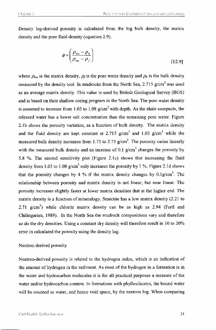
Chapier 2 Pore Pressure Evaluat ion Concepts and definitions
Density log-derived porosity is calculated f rom the log bulk density, the matrix
density and the pore f lu id density (equation 2.9).
0: ( \
Pma ~ Pb
Pn,a ' P f [E2.9]
where pma is the matrix density, Pf is the pore water density and ph is the bulk density
measured by the density tool. In mudrocks f rom the North Sea, 2.715 g/cm was used
as an average matrix density. This value is used by British Geological Survey (BGS)
and is based on their shallow coring program in the North Sea. The pore water density
is assumed to increase from 1.03 to 1.08 g/cm 3 with depth. As the shale compacts, the
released water has a lower salt concentration than the remaining pore water. Figure
2.1b shows the porosity variation, as a function o f bulk density. The matrix density
and the fluid density are kept constant at 2.715 g/cm 3 and 1.03 g/cm 3 while the
measured bulk density increases from 1.75 to 2.75 g/cm 3. The porosity varies linearly
with the measured bulk density and an increase o f 0.1 g/cm 3 changes the porosity by
5.8 %. The second sensitivity plot (Figure 2.1c) shows that increasing the f lu id
density f rom 1.03 to 1.08 g/cm 3 only increases the porosity by 1 %. Figure 2. I d shows
that the porosity changes by 4 % i f the matrix density changes by 0.1 g/cm . The
relationship between porosity and matrix density is not linear, but near linear. The
porosity increases slightly faster at lower matrix densities that at the higher end. The
matrix density is a function o f mineralogy. Smectite has a low matrix density (2.21 to
2.71 g/cm 3) while chlorite matrix density can be as high as 2.94 (Fertl and
Chilingarian, 1989). In the North Sea the mudrock compositions vary and therefore
so do the dry densities. Using a constant dry density w i l l therefore result in 10 to 20%
error in calculated the porosity using the density log.
Neutron derived porosity
Neutron-derived porosity is related to the hydrogen index, which is an indication o f
the amount o f hydrogen in the sediment. As most o f the hydrogen in a formation is in
the water and hydrocarbon molecules it is for all practical purposes a measure o f the
water and/or hydrocarbon content. In formations wi th phyllosilicates, the bound water
w i l l be counted as water, and hence void space, by the neutron log. When comparing
Car l Predrik G v l l e n h a m m a r 21
C hapter 2 Pore Pressure Evaluation Concepis and lietlmiions
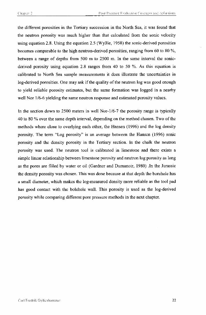
the different porosities in the Tertiary succession in the North Sea, it was found that the neutron porosity was much higher than that calculated f rom the sonic velocity using equation 2.8. Using the equation 2.5 (Wyll ie , 1958) the sonic-derived porosities becomes comparable to the high neutron-derived porosities, ranging f rom 60 to 80 %, between a range o f depths from 500 m to 2500 m. In the same interval the sonic-derived porosity using equation 2.8 ranges f rom 40 to 50 %. As this equation is calibrated to North Sea sample measurements it does illustrate the uncertainties in log-derived porosities. One may ask i f the quality o f the neutron log was good enough to yield reliable porosity estimates, but the same formation was logged in a nearby well Nor 1/6-6 yielding the same neutron response and estimated porosity values.
In the section down to 2500 meters in well Nor-1/6-7 the porosity range is typically
40 to 80 % over the same depth interval, depending on the method chosen. Two o f the
methods where close to overlying each other, the Hansen (1996) and the log density
porosity. The term "Log porosity" is an average between the Hansen (1996) sonic
porosity and the density porosity in the Tertiary section. In the chalk the neutron
porosity was used. The neutron tool is calibrated in limestone and there exists a
simple linear relationship between limestone porosity and neutron log porosity as long
as the pores are f i l led by water or oil (Gardner and Dumanoir, 1980) .In the Jurassic
the density porosity was chosen. This was done because at that depth the borehole has
a small diameter, which makes the log-measured density more reliable as the tool pad
has good contact with the bolehole wall . This porosity is used as the log-derived
porosity while comparing different pore pressure methods in the next chapter.
Carl Fieclrik Gyllenhammar 22

Chapter 2 Fore Pressure (-.valuation Concepts and definitions
i or. I Sonic {Wytlie}- porosity
:i 9 0 S. Hansen - porosity
Density - porosity
I I ; i .«0 Neutron - porosity
LOG - porosity n 7f 1
S 0.60 i
i ! it • 0.50 1 . I
i 0 J i
S 0.30
0 20
0 10
L C no 500 1000 1500 2000 2500 3000 3500 4000 4500 5000
D e p t h ( m R K B )
Figure 2.2 Log derived porosities in well Nor-1/6-7 Norway. The low porosity interval from 3261m to 4346m depth is the Cretaceous Chalk. The values are listed in Appendix 1.
Based on Figure 2.2 it is important to realize the uncertainties that exit in the porosity
estimates in shales based on wireline logs. This put limitations on the conclusions we
may wish to draw concerning the mechanisms underlying the porosity reduction or
compaction. I f one only has available a wireline log-derived porosity profile, one can
clearly not attribute the porosity change solely either to a mechanical process or to a
chemical process.
2.1.3 Normal compaction curve and trend lines
During normal compaction, a mudrock undergoes a monotonic increase in effective
stress, which causes an elastoplastic reduction in porosity. Compaction is a result o f
grain reorientation and breakage. Mudstone consists o f clay minerals, fine grained
quartz, feldspar and mica. As the compressibility is different for different minerals as
well as for different clay minerals, the mudrock compressibility becomes very
diff icult to predict. The resultant relationship between effective stress and porosity is
known as the normal compaction curve (Harrold et al., 1999). In this case equilibrium
is reached such that:
Pf (pore pressure) = phycj (hydrostatic pressure).
Curl Fredrik Gyllenhammar 23

Chapter 2 Pore Pressure b \ alum ion Concept!: and definitions
Although many porosity - depth data have been published, details o f age, lithology or
effective stress are generally absent. In this study it was chosen to evaluate and
compare two different relationships: (1) Athy type and (2) Soil-mechanical type.
These compaction curves assume mechanical compaction only, and are suitable only
to describe siliciclastic sediments. Below 2-3 km depth (70-100°C), mineral
dissolution and precipitation becomes important (Bjorlykke, 1999). At these
temperatures hydrocarbon generation also comes into play. There have been many
publications on attempts to assess the potential overpressure generated by these
reactions. The results are conflicting in the sense that for the same reaction, some
suggest that no overpressure is generated while others suggest generation o f large
overpressure. The conflict lies to a large degree in the assumed permeability. For
many of these reactions to generate overpressure, the permeability w i l l not be low
enough for overpressure to be retained over geological time (Osborne and Swarbrick,
1999). It is also evident that wi th all the uncertainties with regard to chemical
compaction or chemical reactions in mudrocks, it would be quite impossible to predict
the normal compaction trend and hence impossible to calculate the pore pressure.
Chemical compaction w i l l therefore not be taken into account in the present study.
2.1.3.1 Athy-type relationship
The exponential curve to describe compaction was introduced by Athy (1930). It was
based on curve f i t t ing a particular data set and is given as:
Where 0 is porosity at depth o f interest, 00 is porosity at sea bed, c the compaction
coefficient and z the depth. Variations o f the compaction curve result f rom
substituting depth wi th mean or vertical effective stress. The Athy compaction curve
was later modified by Hubbert and Rubey (1959), who recognised that porosity is
controlled by effective stress and not by depth:
0 — 0oe ,(-«) (Athy, 1930) [E2.10]
0 = K + 0oe c [ E 2 . l l ]
Carl Predrik Gvllenhammar 24

Chapter 2 Pore Pressure kvaluation Concepts and ueiimhuns
Where <p is shale porosity, A. is a constant, <fo is the sea bed shale porosity, av is the vertical effective stress in psi and c is the compaction coefficient ranging from 4000 to 7000 (Figure 2.3)..
2.1.3.2 Soil mechanics relationship
A normal compaction trend has been developed by Burland (1990), following
Skempton (1970) based on soil mechanical (SM) experiments:
V^ioo j [E2.12]
where e - fl(l-<p) is void ratio, crv' is the vertical effective stress, (Tioo is the reference
value o f effective stress, taken here to be 100 KPa, eioo is the void ratio at 100 KPa
effective stress, about 10 meters below seabed and Cc is the compaction coefficient.
2.1.3.3 Athy - Soil mechanics: how are they different
The soil mechanics and Athy normal compaction trends are both a function o f void
space and the compaction coefficient. The two fundamental differences are that in the
Athy equation the porosity varies exponentially wi th respect to the effective stress (or
depth) while in the Soil Mechanics equation the effective stress varies exponentially
wi th respect to the void ratio, where void ratio is 0/(1 -())).
The two equations can be rearranged:
SM: av = 0 - l o o x l O ^ ) [E2.13]
Athy: ^ = ^ x e " f f ' c [E2.14]
Mathematically one o f the equations is the inverse o f the other (Figure 2.3).
Figure 2.3 shows the porosity versus the effective stress for the two equations: Athy
and the SM. The two curves would have been symmetric i f the parameters had been
set inverse o f each other. This suggests that the two equations are inverse functions. It
is important to note that the SM compaction trend w i l l cross the depth axis suggesting
that the mudrock porosity w i l l reach 0 %. The Athy compaction curve w i l l never
Carl i-redrik Gyllenhammar 25

Chap Pore Pressure Evaluation Concepts and definitions
reach 0 % porosity, only at infinity. The sea floor porosity is a factor that can be
related to samples. The compaction coefficient is a function o f rock compressibility,
which in theory could be measured in the laboratory (Athy, 1930). But the
compressibility w i l l vary with depth as the rock becomes more consolidated. In
practice what is being done is to use a well where the pore pressure is assumed
hydrostatic based on the M W used and RFT pressure points. Then calculate the
mudrock porosity to calibrate the compaction coefficients in the normal compaction
equation.
Figure 2.3 shows how different the two equations express the change in porosity with
increased total stress. The soil mechanical function suggests a larger rate o f porosity
reduction in the shallow section and w i l l always end up with zero porosity i f the total
stress gets large enough. The Athy function suggests a more moderate change o f
porosity in the shallow section. With increasing stress, the porosity w i l l move
asymptotically to zero porosity, but never become zero.
Normal compaction
Log der ived poros i ty
0.1 0.4
5000
10000
15000
20000 L0
! 25000
" 30000
Athy, 0.7, 0.00008 35000
40000 SM, 2 (0.66), 0.74
45000
50000
Figure 2.3 Comparison of porosity with effective stress for the Athy and the SM equations. Initial porosity (sea floor porosity) for Athy is 0.7 (70 %) while the porosity at 100 kPa (approximately 100 meters below sea floor) is 0.66 (66 %) The compaction factors a re for Athy; 0.00008 and SM; 0.74.
Carl Fredrik Gyllenhammar 26

Chapter 2 I'orc Pressure L valuation Concepts and definitions
100 (porosity in %) 20 40 60 80
Porosity (0
Solidity ° 1.5 Void Ratio
•
0.0 0.2 0.4 0.6 0.8 1.0 1.2 1.4 1.6 1.8 2.0 Void ratio
Figure 2.4 The relation ship between porosity, solidity and void ratio is shown. The y-axis is the compaction as a length reduction. It is assumed that a confined volume is compressed beginning with a void ratio of four.
Figure 2.4 shows the three different frames o f reference to describe the loss o f pore
space. This is a theoretical model built in EXCEL based on the definition o f porosity,
solidity and void ratio. The compaction as length reduction on the y-axis represents
the proportional thickness reduction and the corresponding porosity, solidity and void
ration. Solidity is the volume o f solid grains as a percent o f the total volume o f
sediment, i.e. ( 1 - ())). The complement to solidity is porosity as the volume o f pore
space as a percent o f the total volume of sediment. This is the opposite o f what has
been suggested by Baldwin and Butler (1985). The third parameter is void ratio,
which is the ratio o f the volume of pore space and the volume of solids. Figure 2.4
shows that there is a linear relationship between void ratio and compaction while the
relationship is non-linear between porosity as well as solidity to compaction. It would
therefore be mathematically easier to describe the compaction as a function o f void
ratio rather than porosity. The reason why the oil industry uses porosity is that it has
become the convention in the reservoir section. By comparison the convention in the
soil mechanics environment is to use void ratio as compaction is o f interest.
Carl Fredrik Gyllenhammar 27
2.1.4 Vertical versus mean effective stress
The mean effective stress (crm) is defined as the difference between the mean stress,
sm, which is the mean o f sum of the vertical and the two horizontal principal stresses,
and the pore pressure.
am= sm-pf [E2.15]
where Sm =^(SV +Sh + SH) [E2.16]
with Sf, and SH being the minimum and maximum horizontal stresses, respectively.
The idea o f using mean stress rather than vertical stress is based on the poroelasticity
theory, which suggests that it is the mean stress, rather than the vertical stress that
controls porosity reduction (Goulty, 1998).
When using mean effective stress <rv' is replaced by <rm' in the equation for normal
compaction such as E 2.11 and E2.12.
The vertical or lithostatic stress is calculated by integrating the density log. Sh can be
estimated by assuming it is equal to the leak o f f test (LOT). The LOT pressure is
measured in a short length o f open hole drilled after a string o f casing is cemented in
the well (Engelder and Fischer, 1994). To test the maximum pressure the system can
sustain in an emergency, the convention is to dri l l through the cement below the
casing plus three meters o f new formation. Dri l l ing f lu id is then pumped down hole in
a closed system and the pressure build up is recorded until the formation fractures.
The well is then shut in and the instantaneous shut-in pressure is recorded. Collected
LOT data suggest that the LOT can overestimate the Sh by 5% (Bell, 1990).
Gaarenstroom et al (1993) used LOT data f rom the North Sea and showed that the Sh
is a function o f depth or the overburden. Engelder and Fischer (1994) show that there
is a relationship between Sh and pore pressure. In basins wi th tectonic stress the Sh and
SH w i l l be different. The direction o f SH can be established by studying the calliper log
f rom the well bore. Measuring the predominant borehole breakout directions does
this. Measuring the expansion o f cores during the first hours after being cut can also
Cai l Hedrik Gylienhammai 28

Pore Pressure k valuation C. oncepts and definitions
give this information (Zoback et al., 1985, Evans and Brereton, 1990). As these logs
or cores are rarely available and the methods far f rom generally accepted, Sh and SH
are in this study set equal.
2.2 Pore Pressure Calculation Methods
Pore pressure prediction models can be divided into two major groups; vertical and
horizontal methods (Traugott, 1997). The vertical methods are also called explicit
methods as they assume that given a log value or porosity, the effective stress or pore
pressure can be determined uniquely. This requires also that a normal compaction
trend have been defined. A classical example is the equivalent depth method
(Mouchet and Mithell , 1989) and the "Harrold" method (Harrold et al., 1999).
The horizontal methods (often called ratio method) are based on empirically related
ratio o f the measured parameter to the expected value at a trend line at the same
depth. Methods such as the Eaton (1975) method, Hottmann and Johnson (1965) and
PresGraf (Heppard, et al., 1998) are methods in this category.
The difference between the horizontal and vertical methods is illustrated at Figure 2.5.
I f one assumes that in this case the correct normal compaction curve fa is the Athy
curve (solid red) with regard to the vertical methods the pore pressure at the
equivalent depth would be at A . Wi th regard to the horizontal method the pore
pressure would be calculated as a function o f fa and the value at D . The equation used
is empirically derived (Eaton, 1975).
Carl Frednk Gvlleiihammar 29

Chapter 2 Pore Pressure Evaluation Concepts and definitions
Nxmai osrrpaction
c Log derived porcdty
0,1 0 2 03 G<! 0 5
— *
SCO
toco
1SC0
2LXQ - / A "8 5 £. 2SQ0 / / l 3QC0 -
7 / - • 3050 / / * i / * —— O T .amtm
4X0 / /*' SB.2 pSS.0.7 t
•WCO i /* // *
tocoJ
Figure 2.5. Porosity from a pseudo well is plotted versus depth. Integrating the density log and subtracting the hydrostatic pressure calculate the effective stress. The two normal compaction curves are coming from Figure 2.3.
2.2.1 Vertical Methods
2.2.1.1 Equivalent depth method
The equivalent depth method is based on the effective stress equation for porous
media (Equation 2.1, Terzaghi, 1936). Mechanical compaction o f fine-grained
sediments w i l l , i f the excess pore f lu id cannot escape, result in f lu id pressure
exceeding the hydrostatic pressure. This is often referred to as disequilibrium
compaction (Fertle, 1976, Magara, 1976, Mann and MacKenzie, 1990, Osborne and
Swarbrick, 1997). I f one assumes that no other physical or chemical processes add to
the pore pressure generated, this pressure can be calculated mathematically. The
calculation assumes that the lithology in the overlying succession is uniform and that
Sh and SH are equal. When dewatering is incomplete, mechanical compaction is
incomplete and therefore the porosity reduction is reduced or halted (Swarbrick and
Schneider, 1999). The consequence o f these assumptions is a direct relationship
between the porosity and the effective stress. I f the porosity does remain constant with
increasing depth the effective stress w i l l also remain constant and the pressure f rom
Carl Fredrik Gyllenhammar 30

Chapter 2 Pore Pressure tvaluation Concepts and definitions
the weight o f the lithostatic column between the two porosity points w i l l be the
additional overpressure.
Figure 2.5 shows porosity versus depth wi th two normal compaction trends displayed.
Since the porosity can be calculated f rom the sonic, density or neutron log, the
porosity could have been substituted by any o f these logs and the normal compaction
could have been converted f rom a porosity versus depth relationship to a log response
as a function o f depth. But using the porosity has an advantage i f it is calculated f rom
a combination o f several logs rather than depending on only one input log such as the
sonic slowness.
The following is an example o f how the computation can be made. Phi 1 is at depth 1
on the pseudo well porosity curve where the pore pressure is to be calculated. In this
case the normal compaction trend is an Athy type equation where the porosity is
calculated as a function o f depth. Entering the calculated porosity (or a sonic
slowness) the equivalent depth " A " on the normal compaction trend is found. Since
" A " is on the normal compaction curve the Pf at " A " is the hydrostatic pressure
Phyd(A)- The effective stress in " A " can therefore be calculated using the effective
stress law; <7A = svA - phyd(A) where S v A is the vertical overburden at " A " calculated
f rom integrating the density log. It was assumed f rom the beginning that the effective
stress at phi 1 and A is the same <7A =0^ , . I f follows that; - pf =svA - p h y d [ A )
which can be rearranged to;
Pf =SV~S
VA+ PhyJW [E2.17]
On Figure 2.5, porosity is plotted versus depth. This method is physically correct for
the normal compaction curve only i f the density is constant. Density variations w i l l be
accounted for i f the porosity is plotted versus the effective stress rather than the depth
(Figure 2.6). This is done by integrating the density log and subtracting the
hydrostatic pressure. The normal compaction equation in this case is the effective
stress as a function o f porosity. Entering the porosity at depth 1 into the normal
compaction equation gives the effective stress at depth, " A " which is the same at
depth 1. As the porosity is displayed as a function o f the theoretical effective stress
assuming hydrostatic pressure the pore pressure in 1 is simply the effective stress in 1
Carl Fredrik Gyllenhammar 31

Chapter 2 Pore Pressure Evaluation Concepts and definitions
minus the effective stress in " A " plus the hydrostatic pressure in " A " . This method
w i l l be referred to as the equivalent effective stress method (Mann and MacKenzie,
1990).
0 0.1
Normal oorroadion
Log dented porostj
C = 0 '
- i r
I X i T
i
- M i l
i I aran
1 - I I :
• h : o m nit
Figure 2.6 Porosity from a pseudo well is plotted versus mean effective stress. The two normal compaction curves are coming from Figure 2.3. See text for an explanation for the equivalent effective stress method.
2.2.1.2 Harrold method
A method to calculate pore pressure using wireline log was developed at the
University o f Durham by Toby Harrold (Harrold, 1999). The method involves
plotting porosity as a function o f the mean stress, using a relationship first developed
by Breckels and van Eekelen (1982) coupling pore pressure, depth, vertical stress and
mean effective stress.
The vertical stress sv is calculated by integrating the density log. Sh is calculated using
the empirical relationship derived from well data in Brunei by Breckels and van
Eekelen (1982):
Carl Fredrik Gyllenhammar 32

Chapter 2 Fore Pressure Evaluation Concepts ami definitions
sh=\6.6DlA4i+0A9(pf-phwl) [ E 2 1 g ]
By combining equation 2.18 with the mean effective stress law from basic stress
analysis (Goulty, 1998) the fol lowing relationship can be derived (Harrold, 1999):
pf = 1 6 . 6 £ > ' 1 4 5 + 0 . 5 ^ - 0 . 5 ^ - 1 . 5 ^ , [ m 9 ]
The porosity is initially calculated f rom the sonic travel time using the equation
proposed by Issler (1992). When testing this equation on North Sea sediments the
porosity was derived from equation 2.8 proposed by Hansen (1996). The normal
compaction trend was equation 2.12. Application o f this method to three wells f rom
SE Asia is described in Harrold et al., (1999)
2.2.1.3 Explicit method using the resistivity log
Several methods have been published claiming they do not rely on trend lines, and are
therefore more universal. One o f these methods is called the "Explicit method" and
was published by Alixant and Desbrandes (1991). This method was chosen as the
normal compaction curve is based on the equation 2.12 as in the previous method. A l l
parameters listed are calibrated to the North Sea. The method starts by calculating the
mudstone porosity as a function o f the resistivity and the bound water resistivity. The
bound water resistivity is a function o f formation temperature (Clavier et al., 1984):
R,.,h —
297.6 wl> m 1 76
T [E2.20]
T: formation temperature in °F
The porosity is calculated f rom the fol lowing equation:
\-<f>
(Perez-Rosales, 1975) [E2.21]
G is the geometrical factor set at 1.85 and fa the residual porosity set equal 0.1.
Carl l-redrik Gvllenhammar 33

The above relationship is a new way o f calculating mudstone porosity. A more
conventional way would be the Waxman-Smith (1968) equation:
R, _ a 1
Rw~9" \ + RwBQv [ E 2 2 2 ]
B = equivalent conductivity o f the compensating ions
l-d> Qv=CECx—?-pma
r [E2.23]
(CEC is the concentration o f free ions in the dry clay while, Qv is the concentration o f
free ions in the pore f lu id . Thus BxQv is a measure o f the total conductivity o f the free
ions)
n 1/6-7 Porosity
0.1 0 2
1000
1500
2000
2500
3000
3500
4000
4500
5000 sonic-neutron-density porosity Alexant and Des. Resitivity porosity
Figure 2.7 Comparing the porosity derived from the sonic, density and neutron log with the resistivity derived using the equation 1.37 proposed by Alixant and Desbrandes (1991).
Carl Fredrik Gyllenhammur 34

Chapter 2 Pore Pressure hvaluation Concepts and definitions
The poor agreement between the porosity using equation 2.21 and porosity derived
from the density log is shown in Figure 2.7. The difference in the upper section
averages about 20%. The next step in the Alixant and Desbrandes method is to
convert the porosity to void ratio and use the void ratio in a universal normal
compaction curve. This is a curve quite similar to equation 2.12:
e2 =e , - 7 c . l o g , 0
(a \ i>2
(Perloff and Baron, 1976) [E2.24]
Alixant and Desbrandes (1991) set aev\ equal to 1, which is approximately 100 meters
below sea floor. Based on triaxial compression tests o f shale samples from the North
Sea they suggested the void ratio at the depth is 3.84, which is equal to 79% porosity.
The compression index Ic was measured to 1.1. With these constants the equation 2.24
was rearranged to determine the effective stress:
^ = 1 0 ( e - 3 . 8 4 ) / - / ( . [ 2 2 5 ]
Using the standard Terzaghi relationship (equation 2.1), the pore pressure is then
calculated by subtracting the vertical effective stress from the overburden.
Due to the high porosity calculated f rom the resistivity data in the data f rom Norway,
the calculated pore pressure exceeded the overburden gradient. It was therefore
deemed of little value in comparing it further with the other methods. The strength o f
the method, however, is the normal compaction curve applied. This could be
improved by not assuming its universal character, but let it be a function o f clay
content as suggested by Yang and Apl in (1999). The weakness in the method is the
way porosity is calculated from the resistivity data.
2.2.2 Horizontal methods
2.2.2.1 Eaton Method
Eaton (1972, 1975) established empirical relationships between the logging response
and the pore pressure in the Gul f Coast. Routed in the Terzaghi stress relationship
(Equation 2.1) he defined the pore pressure as a function o f the overburden pressure,
Carl Fredrik Uyllenhammar 35
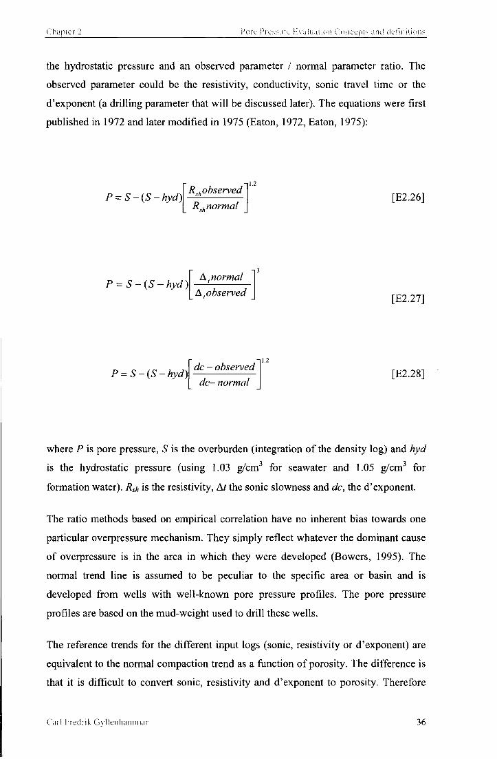
Chapier 2 Pore Pressure b valuation Concents and definitions
the hydrostatic pressure and an observed parameter / normal parameter ratio. The
observed parameter could be the resistivity, conductivity, sonic travel time or the
d'exponent (a dril l ing parameter that w i l l be discussed later). The equations were first
published in 1972 and later modified in 1975 (Eaton, 1972, Eaton, 1975):
P = S-(S-hyd) R ^observed
R ^normal
- i 1.2
[E2.26]
P = S-(S-hyd) A, normal
A,observed
n 3
[E2.27]
P = S - (S - hyd) dc - observed
dc— normal
1.2
[E2.28]
where P is pore pressure, S is the overburden (integration o f the density log) and hyd
is the hydrostatic pressure (using 1.03 g/cm 3 for seawater and 1.05 g/cm 3 for
formation water). Rsh is the resistivity, Ar the sonic slowness and dc, the d'exponent.
The ratio methods based on empirical correlation have no inherent bias towards one
particular overpressure mechanism. They simply reflect whatever the dominant cause
of overpressure is in the area in which they were developed (Bowers, 1995). The
normal trend line is assumed to be peculiar to the specific area or basin and is
developed f rom wells wi th well-known pore pressure profiles. The pore pressure
profiles are based on the mud-weight used to dr i l l these wells.
The reference trends for the different input logs (sonic, resistivity or d'exponent) are
equivalent to the normal compaction trend as a function o f porosity. The difference is
that it is diff icul t to convert sonic, resistivity and d'exponent to porosity. Therefore
d t i l Fredrik Gyllenhumniar 36

Chapter 2 I'orc Pressure kvaluaiiun Concepts and demntions
the normal trend for the different log parameters such as sonic, resistivity and the
d'exponent are established by overlaying the log values f rom multiple exploration
wells in areas where the mud-weight suggest that the mudstone have hydrostatic pore
pressure (Hottmann and Johnson, 1965)
2.2.2.2 The pore pressure calculation program; PresGraf
Several computer programs designed to calculate the pore pressure in mudrocks are
commercially available such as Predict from Knowledge Systems. PresGraf is another
program designed and written by Traugott, M (University o f Durham) and Heppard,
P. (BP). The program is proprietary to BP Exploration, but was made available to this
study by BP. The program has several calculation methods available including the
Eaton method, the equivalent depth method and the PresGraf method. The PresGraf
method is an Eaton type equation only with a different exponent. A l l calculations
were performed using a normal compaction curve proprietary to the program owners.
Some of the principles behind the normal compaction in PresGraf have been
published by Heppard et al (1998).
2.2.2.2.1 PresGraf normal compaction trend
The PresGraf software developed by Amoco uses sonic slowness or the resistivity in
shales as the input variable to calculate the pore pressure in the shales (Heppard et al.,
1998). The normal compaction trend used was developed by Hubbert and Rubey
(1959) (equation 2.11). The pore pressure is calculated as a function o f either the
sonic log or the resistivity log. The normal compaction curve is converted to slowness
(^sec/ft) using the fol lowing equation (Eberhart-Philips et al., 1989);
Vp is the compressional wave in milliseconds per kilometre; Vcl the fraction o f the
volume o f clay and the effective stress is in bars. The volume o f clay in mudstone
varies, but due to the program design it must be entered as an average. This value can
be found be laboratory analysis o f mudrock samples or calculated from various
wireline logs, such as the gamma ray log or a cross plot o f the neutron-density log.
Carl Prechik Gyllenhammar 37
Vp = 5.77 - 6.94(2) - 1 J3yfVcl + 0.446(<7, - e ) [E2.29]

Chapter 2 Pore Pressure Evaluat ion Concepts and definitions
The conversion of the normal compaction trend expressed as a function of porosity to
a function of the resistivity has its root in the dual water model. The duel water model
suggests that clays contains a mixture of two waters (Clavier et al., 1984); the bound
water Sb of conductivity Q,, and the free water of conductivity Cw. The effective water
conductivity Cwe for 100 % water saturation is then;
The Sb is a function of the cation exchange capacity (CEC) with units expressed in
milliequivalents/gram (meq/g). The CEC is a measure of the available free cations.
The CEC in a clay is the ability of a clay mineral to absorb cations from surrounding
waters and maintain them in an exchangeable state. This ability arises because
imperfections in the clay lattice create electronegative charges on the clay surface
(van Olphen, 1963, Grim, 1968) The conductivity of a clay is directly related to the
cation exchange capacity. By knowing the density and porosity the CEC can be
expressed as milliequivalents per unit volume (meq/cm3) of pore fluid; Q. The amount
of bound water (W) has been measured in the laboratory and the following empirical
relationship was found (Hill et al., 1979);
where C is the concentration of sodium chlorides (moles/liter). This leaves us with the
following important relationship;
The specific counterion conductivity in the bound water is measured in mho/m per
meq/cm3 and called B. The quantity of B has been determined (Waxman and Smits,
1968) from core measurements to 2.05 mho/m at 25°C. The conductivity of the bound
water can therefore be expressed as;
cwe = cw{\-sh)+cbsb [E2.30]
W = 0.55 + 0.084VC [E2.31]
Sb = WxQ [E2.32]
Cb-B I W [E2.33]
Combining equation 2.32 and 2.33 gives;
SbX Cb = B x Q [E2.34]
C a r l I-redrik GyHenhamrnar 38

Chapter 2 Pore Pressure Evaluat ion Concepts and definitions
Archie (1942) determined experimentally using clean sandstone the following
equation;
a Ct
[E2.35]
where the Sw is water saturation, Rw the resistivity of formation water and R, the
Void Ratio • ' 5
• v
b 00
• o no
20 00
/ 25
-
v.r..-,
Atf.y r(eff stress). 0.000025.0.55
' . o n
Figure 2.8 The PresGraf normal compaction trend to the left compared with the Athy normal compaction curve (Figure 2.3) to the right.
resistivity of the rock measured by the resistivity tool. The constants are «, a, and m.
These can be found by cross plotting log of the porosity versus log of the RolRw ratio.
n is the saturation exponent, m is the cementation exponent and is equal to the slope
of a best-fit line on the cross plot, a is the value of the Ro/Rw ratio at 100% porosity.
Laboratory experiments suggest that m vary from 1.8 to 2 in consolidated sandstones
(Doveton, 1985). Dewan (1983) suggested that n is equal 2 and a equal 1 in sandstone
mixed with clay. By entering those values (including m-T) into equation 2.35, it
simplifies to;
C a r l Fredrik G y l l e n h a m m a r 39

Chapter 2 Pore Pressure 1£valuation Concepts and definitions
[E2.36]
The following equation is the dual water model for sandstone with clay (Clavier et al.,
In wet shale with no hydrocarbons, Sw is 1. In PresGraf it is assumed that all water in
the claystone is bound. Consequently the total conductivity in the shale is Q,. This
assumption simplifies the equation to;
Having computed a normal compaction trend as a function of porosity, it is possible
to compute one as a function of resistivity knowing the values of the following
variables; Vcl, m and CEC. "m" ranges from 1.6 to 2 in clean formations, but was
found to increase with shaliness reaching values as high as 2.9 in shales (Waxman and
Thomas, 1972).
2.2.3 Seismic
Determining pore pressure from seismic interval velocities is no different than using
the sonic log. The important difference is that the interval velocities that are
calculated from the RMS velocities coming from stacking velocities are horizontal
velocities while the sonic log is measuring the vertical velocity assuming the well is
vertical. There is also a considerable difference in the frequencies. While the seismic
frequency is broadband in the low frequency part of the spectrum (50 Hz), the sonic
log uses 50000 Hz. In general the seismic velocities are 10% faster than the sonic
velocity. In general it is important to understand that velocity anisotropy can play an
important roll and introduce error in the porosity calculation that depend on those data
as input. It is not evident which is the best with regard to calculating the porosity. The
vertical, the horizontal or the average. I f the compaction trend is a function of vertical
velocity it is important to make sure that the shale velocity is the same.
1984);
2 c=s:*r c H , ( i - - f ) + c „ x w w [E2.37]
m m C. = <pmxC,xS d>m xBxQ [2.38]
C a r l Freclrik GyI lenhammur 40
Chapter 2 Pore Pressure E valuation Concepts and definitions
Pennebaker (1968) was one of the first authors to describe in detail how to calculate
pore pressure from seismic velocities. In seismic processing the interval velocities are
calculated from the stacking velocities. This interval velocity is in theory an average
of the sonic log and its application is identical to that of a sonic log. It has the
disadvantage of lacking resolution but the advantage of being acquired prior to
drilling. I f the velocity is from a 3-D seismic survey, a 3-D image of the pore pressure
can be produced.
In the last few years it has been shown that it may be possible to calculate the porosity
from seismic attributes (Elsayed and Slusarczyk, 2001). Several of the seismic
software providers have developed artificial neural networks to extract porosity from
seismic attributes, such as Hamson Russall.
2.2.4 ShaleQuant
The computer program ShaleQuant was developed at University of Newcastle. Shale
samples from the North Sea and the Gulf of Mexico were analysed and their
corresponding wireline log response such as calliper, resistivity, gamma ray, sonic
and density recorded against depth. The underlying premise is that the principal
control on compaction of shales is clay fraction (Aplin et al., 1995). The sample grain
size distribution as clay fraction rather than clay volume and its corresponding wire
line log values were used to train an artificial neural network (ANN). The clay
fraction is a grain size terminology and clay is defined as material with grain size less
than 2 micro metres. The normal compaction curve was equation 2.12 where the
constants are a function of the measure clay fraction from ANN. The pore pressure is
calculated using the equivalent mean effective stress method (chapter 2.2.1.1).
2.2.5 Principle Component Analysis
The multivariate statistical method of Principle Component Analysis (PCA) can be a
useful tool to test each variable importance with respect to any common trend. Any
variable with limited influence on the common trend of change can be identified and
taken out of the analysis. A Principal Component Analysis of the data set will
determine the perpendicular axes (called eigenvectors), which are defined by the
dimensions of the data set. There will be the same number of axes as
variables/dimensions; the longest axis is the First Principle Component (PCI), the
C a r l Fredrik G y l l e n h a m m a r 41

Chapter 2 Pore Pressure h valuation Concepts and definitions
next major axis is the Second Principle Component (PC2), etc. I f there where only 3
variables one could visually see the predominant trend in the data. With N variables
the data points become a cloud in N dimensions and PCA rotates it such that the
maximum variability is visible. Each variable in the analysed data set can be assessed
concerning its contribution to the overall distribution of the data set. A high
correlation between PCI and a variable indicates that the variable is associated with
the direction of the maximum amount of variation in the data set.
Conversely, i f a variable does not correspond to any PC axis, or corresponds only
with high-number PC axes, this usually suggests that the variable has little or no
control on the distribution of the data set. Therefore, Principle Component Analysis
may often indicate which variables in a data set are important and which ones may be
of little consequence. Some of these low-performance variables might therefore be
"weeded out" and removed from consideration in order to simplify the overall
analyses.
The first stage in the process is to standardize the data. The mean and the standard
deviation for each variable is determined using EXEL. Subtracting the mean and
dividing by the standard deviation find the standardized value. Thus the centroid of
each data set is zero.
It is possible to run PCA without dividing by the standard deviation and run an
eigenanalysis of the covariance matrix. But in this case (wireline data) where the
variables are all measured in different units only a correlation matrix can be used. The
entire variable will then have a variance equal to 1.0. The logs included in the analysis
were; delta calliper (delta ca), neutron (HCNC), density (HDEN), gamma ray (HGR),
resistivity (HRD) and the sonic travel time (HAC). The same methodology will apply
to the PCA performed on the drilling data later in this chapter.
Table 2-1 Eigenanalysis of the correlation matrix
Eigenvalue 2.8762 1.3671 0.8951 0.6499 0.1476 0.0642
Proportion 0.479 0.228 0.149 0.108 0.025 0.011
Cumulative 0.479 0.707 0.856 0.965 0.989 1.000
Car l Fredrik Gy l i enhammar 42

C h a p u Pore Pressure hvaluauon Concerns and definitions
V a r i a b l e
D e l t a Ca
PCI PC2
-0.196 -0.478
PC 3
0 . 646
PC4 PC 5
-0.558 -0.028
HCNC 0.556 0.025 0.048 -0.169 0.740
HDEN -0.556 -0.002 0.072 0.208 0.664
HGR 0.100 -0.700 0.077 0.672 0 . 004
HRD -0.131 -0.497 -0 .752 -0 .405 0.082
HAC 0.562 -0.184 0.060 -0.035 -0.067
Scree Hot of Delta Ca-HAC
(D "3
C 0 g> Lu
Component Number
Figure 2.9 Scree plot of the eigenvalue of each principal component of the PCA of the wireline logs.
The scree plot (Figure 2.9) shows how the eigenvalue drops from PCI to PC6 (Figure
2.9). The first screening of the data is done at this level. It is important to make a
decision about what criteria to use with regard to which principal component is
important or not. The Kaiser criterion suggests that we can only retain factors with
C a r l Fredrik G y l l e n h a m m a r 43

Pore Pressure E \ a l u a t i o n Concepts and definitions
eigenvalues greater than 1 (Kaiser, 1960). In this case we would only retain PCI and
PC2.
The scree test is a graphical method first proposed by Cattell (1966). Cattell suggested
using the scree plot to find the place where the smooth decrease of eigenvalues
appears to level off. In this case it is not evident whether to include PC3 and PC4 in
addition.
PCA1
j ^ " j i i f f l t i i i u
- 1 0 -
-15 -
- 2 0
25 PCA1
• i H D E N 9-
-0.1
-0 .2
-0.3
-0 .4 D C A L I
-0.6
-0.7
-0 .8
PCA1
r - ~ - - 0.8 -
D C A L ^ . 6 -
0.4 -
0.2 -
A H D E N 0
^ H G R ^ A C
1 -0.5
-0.2 -
-0.4 -
-0.6 -
-^K -
' H C N C 1 0.5
Figure 2.10 a, b, c and d. The plots to the left (a and c) are cross sections through data perpendicular to P C I , PC2 and PC3. b and d show the loading values with respect to the different principal components.
Table 2.1 includes the loadings of the principal components. The loadings can also be
presented graphically (Figure 2.10b and d). The loadings for PCI shows that the
density and neutron measurements have 0.55 loading in opposite directions and that
the sonic measurements have a positive 0.56 loading. Calliper, gamma ray and
resistivity have limited influence on PCI but are the most influence on PC2 and have
loadings in the same direction. These three measurements are also controlling PC3
and PC4. Figure 2.10 a and c are cross sections through the PCI and PC2. The blue
C a r l Fredrik G y l l e n h a m m a r 44

Chapter 2 Pore Pressure I: valuation Concep i s and definitions
cloud comprises the Tertiary data points while the red cloud is the Jurassic data. It
suggests that there is some sort of parallel shift of the general trend at Figure 2.10a.
This may be due to the chalk layer in between or an erosional discontinuity between
the two epochs. Figure 2.11 shows the PCI versus depth in blue and the log-derived
porosity in green. It is possible that the PCI is the porosity change with depth, and
that the porosity can only be calculated from the density, neutron or the sonic log. The
three other including resistivity represent only noise in relation the PCI. With respect
to PC3, the gamma ray has no impact just like the density, neutron and sonic. The
delta calliper and resistivity pull with equal amount in opposite direction. This
suggests that the variation in hole size has most impact on the resistivity log. It puts
the resistivity log into a very difficult position with respect to whether it can be used
to calculate the pore pressure based on Eaton's equation or equivalent depth where in
effect it substitutes for sonic or density measurements.
It is important at this stage to remember than the study so far has been concentrated
on data from one well, Nor 1/6-7 and not to generalize these observations beyond this
well. But it shows the power of PCA as an analytical method, which should be done
more regularly on well data.
Cal l hredrik G y l l e n h a m m a r 45

Chapter 2 Pore I ' rcss i i iv Eva lua t i on Concept-- and d e f i n i t i o n s
PCA1 P C 1
! C 0 I
• n o o
15 0 1 5 0 0
, 1-OC
3 0 0 0 | 3 0 0 0
1 5 0 0
4001
j •: • o 4 5 0 0
5 0 0 0
Figure 2.11 a and b. PCI versus depth in blue and the sonic travel time in green.
2.3 Drilling parameters
Most of what is explained in this chapter is based on the author's personal experience
from having been a mudlogger for 18 months followed by 10 years as a wellsite
geologist with responsibility for pore pressure evaluation using drilling parameters.
The drilling parameters come from three sources; the mudloggers, MWD engineers
and the driller. The mudloggers data are divided into two categories; real time data
and lagged data (table 2.2). The LWD/MWD tool is a group of sensors equivalent to
the wireline sensors built into the drill-string placed just behind the drill-bit. The
signals are transmitted to surface by pressure pulsation in the mud, as well as being
recorded in a memory built into the tool. As the sensors can be several meters behind
the drill-bit the data are regarded as lagged data, i.e. the recording of the data does not
correspond in time with the position of the bit, and hence the drilling response. The
MWD/LWD data as pore pressure indicators are not discussed separately as the data
are regarded close to identical with wireline data. (Chapter 2.2). The driller's data are
all real time. Since they are recorded by the mudloggers as well, only data from the
mudloggers will be listed as drilling parameters.
C a r l Fredrik Gyl lenhani inar 46

Chapter 2 Pore Pressure Evaluation Concepts and definitions
Table 2-2 A list of measurements that can be used to interpret the shale pore pressure.
Mudlogger real time Mudlogger lagged
data MWD data Drillers data
d'exponent gas resistivity mud flow in (kick)
torque mud temperature density pit gain (kick)
mud flow in (kick) mud salinity neutron porosity drill break
pit gain (kick) cuttings shape sonic porosity pump off mud
return
changes in
standpipe pressure cavings pit loss
pit loss cuttings density
mud density in/out
On most drilling sites all mudloggers and drillers data are available, but the use of
MWD/LWD tools varies a lot due to high rental cost of the tools. In addition most
operators wil l wireline log each section drilled and will therefore get the data only
later. While available during drilling they are very useful, but should be avoided as
the primary resource. Base on personal field experience these tools often fails and the
drill string will have to be pulled to surface for repair (a bit trip). As this operation
often takes 24 hrs. it is normally only done when a drill-bit is worn, hence the name
"bit trip".
Since the interpretation of the wireline data and hence the MWD/LWD data have
been discussed (Chapter 2.2), it was decided not to include them in this section. One
can also see from table 2.2 that the drillers data are duplicated as the same data are
collected by the mudlogger although the data are sourced from different sensors. The
drilling data discussed in this chapter are therefore divided into two groups; real time
data and lagged data as listed in column one and two of table 2.2.
Car l Fredrik G y l l e n h a m m a r 47

Chapter 2 Pore Pressure Lvaluat ion Concepts and definitions
2.3.1 Real time data
Real time data are all recorded by the mudlogger which represents the data recorder
from the actual total depth of the well; rate of penetration (ROP), weight on bit
(WOB), bit revolution per minute (RPM), d'exponent, torque, mud flow in, mud loss,
changes in standpipe pressure and PWD (down hole mud pressure measured by the
MWD or LWD tool.
2.3.2 D'exponent
The d'exponent is a way of normalizing the rate of penetration (ROP) to extract the
formation drillability or hardness. Bingham (1964) suggested the following
relationship between ROP, weight on bit (WOB), bit rotating speed (RPM) and bit
diameter (D):
ROP/RPM= a (WOB/D) d [E2.38]
where d is the compaction exponent and a the lithology constant. Jordan and Shirley
(1966) solved this equation. They assumed constant lithology in a shale sequence,
hence a=l:
log10(ROP/RPM)=d(log10(WOB/D)) [E2.39]
This equation was rearranged to:
DEXP=log,0(ROP/60RPM)/logio(WOB/106D) called the d'exponent.
In standard metric units, ROP is in meters/hour, RPM in revolutions/minute, WOB in
tones and D the bit diameter in inches. In standard US units ROP is in feet/hour, RPM
in revolutions/minute, WOB in pounds and D the bit diameter in inches.
C a r l Fredrik G y l l e n h a m m a r 48
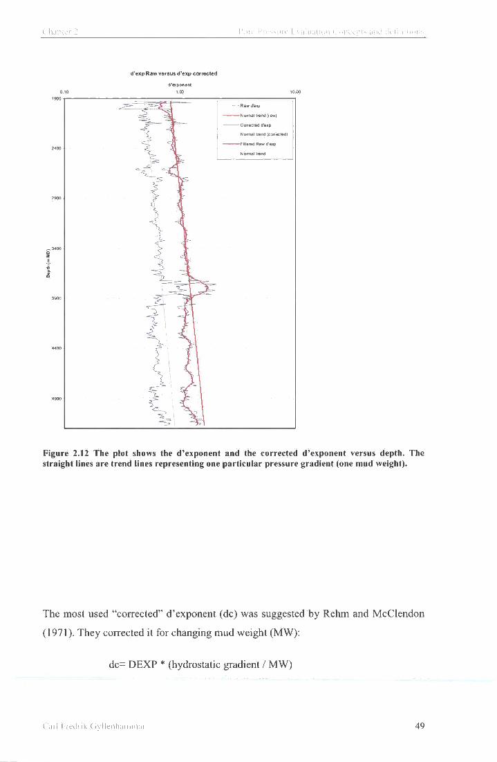
0.10
1900 i
d ' e x p R a w versus d'exp corrected
d'eaponent
1.00
Raw d'exp
Normal trend (raw)
Corrected d'exp
Normal trend (corrected)
F Itered Raw d'exp
Normal trend
Figure 2.12 The plot shows the d'exponent and the corrected d'exponent versus depth. The straight lines are trend lines representing one particular pressure gradient (one mud weight).
The most used "corrected" d'exponent (dc) was suggested by Rehm and McClendon
(1971). They corrected it for changing mud weight (MW):
dc= DEXP * (hydrostatic gradient / MW)
C a r l Fredrik G y l l e n h a m m a r 49
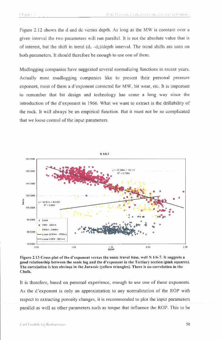
Chapter 2 Pore Pressure h \ a l u a t i o n Concept 1 - and d e f i n i t i o n s
Figure 2.12 shows the d and dc versus depth. As long as the MW is constant over a
given interval the two parameters wi l l run parallel. It is not the absolute value that is
of interest, but the shift in trend (di -d2)/depth interval. The trend shifts are seen on
both parameters. It should therefore be enough to use one of them.
Mudlogging companies have suggested several normalizing functions in recent years.
Actually most mudlogging companies like to present their personal pressure
exponent, most of them a d'exponent corrected for MW, bit wear, etc. It is important
to remember that bit design and technology has come a long way since the
introduction of the d'exponent in 1966. What we want to extract is the drillability of
the rock. It will always be an empirical function. But it must not be so complicated
that we loose control of the input parameters.
N 1/6-7
y = -37.Q86x + 191.12 R ! = 0.7904
y= 16.301X +83.762 R ! = 0.095
• Chalk
• 1000 - 3261m
• 4346m -5000m
— Linear (4346m - 5000m)
linear (1000 - 3261m) o
1.50 DEXP
Figure 2.13 Cross plot of the d'exponent versus the sonic travel time, well N 1/6-7. It suggests a good relationship between the sonic log and the d'exponent in the Tertiary section (pink squares). The correlation is less obvious in the Jurassic (yellow triangles). There is no correlation in the Chalk.
It is therefore, based on personal experience, enough to use one of these exponents.
As the d'exponent is only an approximation to any normalization of the ROP with
respect to extracting porosity changes, it is recommended to plot the input parameters
parallel as well as other parameters such as torque that influence the ROP. This to be
C a r l Fredrik G y l l e n h a m m a r 50

able to visually check i f a sudden change in one of the input parameters is the source
to a trend shift in the d'exponent.
The d'exponent was developed using rock bits, while PDC bits are often used today.
A PDC bit do not have any roller cones, but is a solid cutter that cut loose the rock
rather that hammer loose the rock bits. It appears that the d'exponent still can be used,
but the data is more scattered. The d'exponent is also a function of what type of drill-
bit being used and the size and number of drilling stabilizers used.
Figure 2.13 show a good correlation between the d'exponent and the sonic value in
the Tertiary section. This suggests that the d'exponent is also a function of porosity
and should in theory also be a function of pore pressure. Figure 2.14 show that there is
no correlation between the d'exponent and the resistivity log.
N 1/6-7
10.0000 i 1 f
• Chalk 9.0000
• 1000 - 3261m
B.OOOO o o 4346m - 5000m
7.0000
6.0000
S 5.0000
4.0000
At 4% ' * 3.0000
2.0000
1.0000 r . 1
0.0000 0.50 1.00 1.50 2.00 2.50
DEXP
Figure 2.14 Cross plot of the d'exponent versus the resistivity log. The plot show no correlation.
One important limitation is that a reduction of the overpressure cannot be measured
and often not even detected. The mud weight (MW) needed in one section drilled
(between two casing shoes) wil l always be a function the highest overpressure
gradient encountered. Drilling with higher MW than needed (drilling overbalanced)
will to some degree reduce and change the ROP, but often not at all. Small changes in
Car l F r c d n k G y l l e n h a m m a r S i

Chapter 2 Pore Pressure Evaluat ion Concepts and definitions
lithology can be important for the particular bit in use and increase the ROP
regardless of reduction in overpressure.
Table 2-3 Eigenanalysis of the correlation matrix
Eigenvalue 1.5075 1.0032 0.4893
Proportion 0.502 0.334 0.163
Cumulative 0.502 0.837 1.000
Variable PCI PC2 PC3
ROP 0.708 0.004 0.706
RPM 0.347 0.869 -0.352
WOB -0.615 0.494 0.614
The eigenvalues of the principal components in table 2.3 show that it is PCI and PC2
that have an eigenvalue higher than 1 and that PCI (Figure 2.15) represent 50% of the
variability while PCI and PC2 account for 84% of the variability. PCI is influence by
the ROP and the WOB pulling in opposite direction while the RPM more or less
represent noise on PCI (Figure 2.16b).
C a r l Fredrik G y l l e n h a m m a r 52
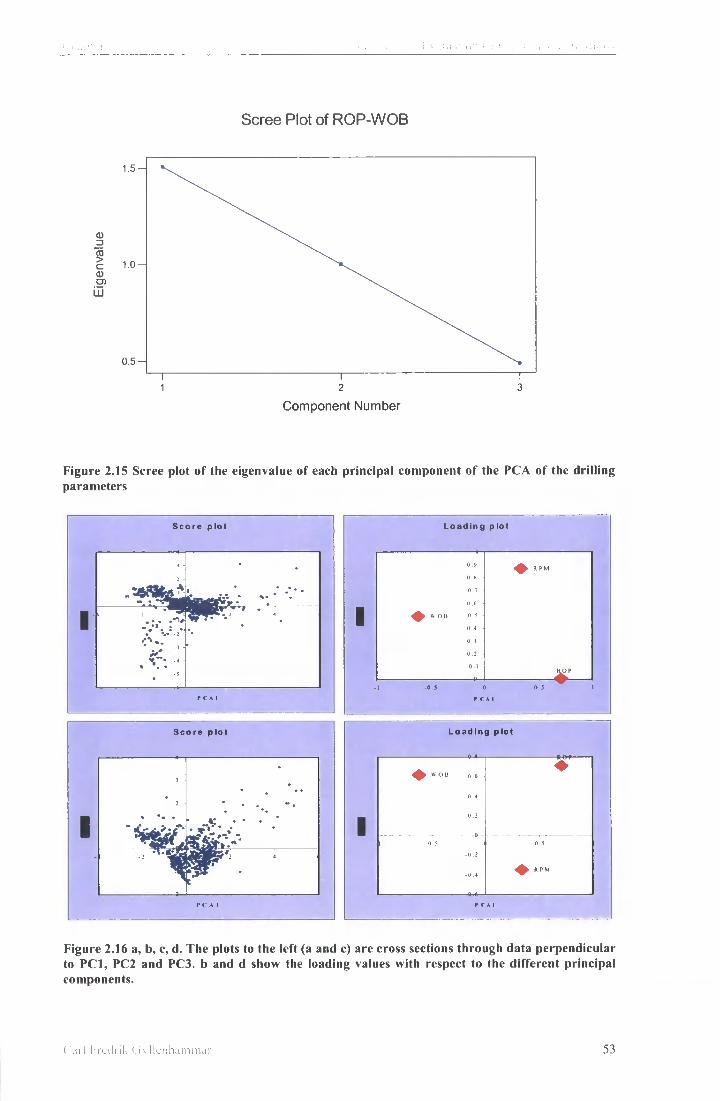
Scree Plot of ROP-WOB
Component Number
Figure 2.15 Scree plot of the eigenvalue of each principal component of the PCA of the drilling parameters
S c o r e p l o t
I
I
i -
• " . * - • • • —
1 -2
- ** • -• • • •
* \ >* . V . *
K i t ' * ' . w ** •
S c o r e p l o t
3
• • •
K • * • *
P C A 1
L o a d i n g p l o t
L o a d i n g p lo t
Figure 2.16 a, b, c, d. The plots to the left (a and c) are cross sections through data perpendicular to P C I , PC2 and PC3. b and d show the loading values with respect to the different principal components.
f ' u i l F r e d i i k C i y l l e i i h a m m u r 53

The loading plot and score plot of PCI versus PC2 suggest there is a predominant
trend controlled by ROP and WOB (Figure 2.16). Figure 2.17 show the PCI versus
depth with the log derived porosity and the sonic log overlaid. I f we assume it is the
degree of consolidation we try to get from the drilling parameters it appears from this
well that the RPM do not help. The d'exponent i f for pore pressure analysis would be
a better pore pressure indicator in this well i f it were only a function of ROP and
WOB.
PCM ctilling parameters versus KA1 PCM dilling versus narnaized normalized sonic value poraaty
PCM PCM PGM
0 6 0
!'U) 1500
2300' 1 ' W
w 1
us f.i I
40m '1030 4030
If*. 450̂ «'
6889 *5
Figure 2.17 a, b and c. PCI versus depth with the standardized log porosity overlaid in Figure b and the normalized sonic travel time in Figure c
2.3.3 Torque
Torque is measured on the surface and represents therefore the sum of the bit torque,
the stabilizer torque and the drill string torque. As the hole gets deeper the contact
Carl I rednk Civllcnhammai' 54
Chapter 2 Pore Pressure livaluation Concepts and definitions
area between the drill string and the borehole walls increases. A sudden increase in
the torque can be related to increased pore pressure, but also be related several other
causes such as;
-swelling clays due to chemical reactions between the formation and the drilling fluid
(mud).
-accumulation of cuttings in the hole because the drilling fluid properties changes and
its lifting capacity is reduced (Mouchet and Mitchell, 1989).
-to rapid building of borehole angle
Torque has for these reasons never been taken directly into account as part of the
normalized ROP equation because the bit torque has not been available. Torque as a
pressure indicator is therefore quite elusive and only used as an addition indicator by
very experienced pore pressure engineers at the wellsite when on are quite certain that
it is only an increase in pore pressure that is causing the increased torque.
Today bit torque can be measured as part of the MWD service. No equation is
available at the time of writing this chapter, but may be an interesting future pathway
when sufficient data becomes available.
2.3.4 Hydraulics
The effect of hydraulic flow on ROP varies for different lithologies as well as degree
of consolidation (Mouchet and Mitchell, 1989). The effect is also a function of MW,
mud viscosity, mud composition, bit type and bit nozzle size. The effect of hydraulic
flow on ROP is not fully understood and cannot be taken directly into the normalized
ROP equation.
2.3.5 Bit type and wear
The d'exponent was developed the tri-cone bits where the only available bit type.
With the introduction of the PDC bit it has been observed that the d'exponents tend to
scatter and its resolution is therefore severely reduced. It is time to develop a new
drilling exponent for the PDC bit, but a good digital database must be available. As
Carl Fredrik Gyllenhammar 55

Chapter 2 Pore Pressure 1: valuation Concepts and definitions
good practices are in place with regard to wireline data, the same is not the case with
regard to drilling data.
Most mudlogging companies has developed some sort of bit wear function that can be
used to correct the d'exponent, but in most cases it confuses more than it helps. Most
drilling supervisors will have experienced that the bit appears to wear out quit sudden
rather than gradually. The result is a sudden drop in ROP due to bit wear rather than a
gradual reduction in the ROP.
2.3.6 Lagged data
Lagged data are the information the mudlogger extract from the drilling mud as it
reach the surface and passes over the shale shaker. This information arrives typically
one to two hours after the bit passed that specific depth. The lagged data can be
subdivided into information from the mud and from the cuttings.
MUD: total gas, mud temperature, mud weight, mud resistivity
CUTTINGS: density, CEC, calcimetry, cuttings gas, shape of the cuttings and
cavings, the volume of cavings.
2.3.6.1 Gas
The gas is sampled from the returning drilling fluid and analysed. This is a
fundamental analysis for safety, and it is for example one of the parameters that NPD
in Norway require be monitored while drilling. As a pore pressure detection tool
while drilling it has the disadvantage of being a lagged parameter and not real time as
the d'exponent.
The total gas is detected in the returning drilling fluid (heather tank) before the shaker
screens. The sample equipment is working under extremely harsh conditions. These
systems need therefore a lot of maintenance and regular calibration. This has proven
very difficult while drilling exploration wells. The different sample equipment are not
standardized and seldom built for purpose. As a result gas level variations are often a
result of change in sampling conditions. The sample equipment is placed in the header
box in front of the shaker screens. Variations in the mud level and frequent cleaning
Carl Fredrik Gyllenhammar 56

Chapter 2 Pore Pressure Evaluation Concepts and definitions
with large quantities of drill water dilute the drilling fluid and results in unreliable gas
readings.
The total gas is also dependent on the volume of drilling fluid a given amount of rock
is cut and diluted into. This ratio dependent of the volume of rock being drilled versus
the volume of drilling fluid it is diluted into is often omitted in the assumed total gas
reading.
The total gas measured is the sum of the gas diluted in the mud from the rock being
crushed by the bit and the gas seeping in from the borewall (gas influx). The total gas
can be categorized according to different sources (Mouchet and Mithell, 1989);
Cuttings gas released from the cuttings while being pumped up hole to surface.
Produced gas seeping in from the borehole.
Recycled gas in the drilling mud system.
Contamination gas from petroleum products mixed into the mud.
The total gas is used as a pore pressure tool based on the idea that i f underbalanced,
gas will seep into the well. I f overbalanced it wil l not. While pumping, the effective
pressure of the mud column against the borewall (ECD) is higher than when the mud
is static. The pumps are turned off while doing a connection or simply a dummy
connection. I f there is a difference between the connection gas (and/or trip gas) and
the background gas, the difference could be due to underbalanced drilling. I f this
difference decreases after increasing the MW we know increasing pore pressure
gradient caused it. But increase of the TOC in the mudrock can easily be mall
interpreted as pore pressure increase as well as a hydrocarbon discovery.
Despite errors in the method, it remains often as the most important method while
drilling. This could be because everyone working at the wellsite regardless of
background can have an opinion about the pore pressure based on this method. When
large changes are observed in the total gas, the drilling engineers and drilling foreman
wil l build their own opinion regarding the pore pressure.
Carl Fredrik Gyllenhammar 57

Chapter 2 Pore Pressure hvaluation Concepts and definitions
2.3.6.2 Cuttings and Cavings
At wellsite the interpreted lithological log is based on describing the drill cuttings.
The bulk sample from the shaker screens are sieved based on a size that is assumed to
be representative of drilled cuttings. Large cuttings (>lcm) are generally regarded as
cavings. Drilling a borehole creates stress at the walls. There will therefore always be
some cavings in the samples. But an increase in the amount of cavings in the bulk
sample is indicative of borehole instability. Abundant cavings are either due to stress
relief (rock mechanical problem) or underbalanced drilling (pore pressure problem).
With regard to pore pressure it is cavings of shales we are most concerned with and
they react with the drilling fluid and changes their original shape as they are pumped
up with the mud. Pore pressure produced cavings are typically long, splintery and
occasionally concave. Stress relief cavings are blockier. But often increasing the MW
solves the problem regardless of the cause (Mouchet and Mitchell, 1989).
Several rock mechanical experts are convinced that cavings will always appear i f one
is under balanced.
2.3.6.3 Mud temperature in and out
The theory behind measuring the mud temperature in and out for pore pressure
evaluation is trying to measure the geothermal gradient. As a result of higher porosity,
hence higher water content high porosity rocks are insulating bodies with regards to
low porosity rocks. One would therefore expect the mud temperature increase less
than before in the pressure transition zone, but increase quit dramatic within the
overpressure zone. In reality this is mostly a method to be used on onshore wells. On
offshore rigs the mud are cold while being pumped up the riser from the seafloor to
the rig. On deep-water wells the method cannot be applied.
2.3.6.4 Mud resistivity in and out
In normally compacted shales water salinity could increase with depth. Overton and
Timko (1969) have demonstrated the role of ionic filtering by clays. This was later
revised by Magara (1978). It is still a controversial question whether the compacting
mudrock act as a filter when water is expelled. It is therefore difficult to assess the salt
concentration in any water flowing from the formation into the borehole. It is also
Carl Predrik Gyllenhammar 58

Chapter 2 Pore Pressure Evaluation Concepts and definitions
difficult to assess the expected salt concentration in the mudrock itself, as that is also
a function of the mudrock mineralogy, which is never available at an exploration
wellsite.
To be able to measure a salt influx into the drilling fluid system it must be a
significant salt contrast between the drilling fluid and the influx. This will require a
near fresh water mud. The North Sea and the Gulf of Mexico have several formations
with high level of Montmorillonite. To inhibit the swelling reaction considerable
amount of KCL is added to the drilling fluid. It is therefore practically difficult to
measure a resistivity change caused by formation fluid influx.
2.3.7 Mud chemistry and mud-formation chemical reactions
The chemical composition of the mud system used is imperative as some water-based
systems can cause swelling of the formation. For example a Montmorillonite rich
formation can swell with out proper shale inhibitor added to the system. This will
increase the torque and reduce drill rate (ROP). The d'exponent wi l l decrease or
remain unchanged suggesting no pressure increase, while the increased torque may
suggest increased pressure. The result is severely reduced resolution on the real time
pore pressure parameters. This is generally a problem in shaly succession with a high
CEC value. It is therefore wise to monitor chemically the CEC well using for example
the Methyl blue titration technique and have the mud composition adjusted to the
zone of highest CEC value for the specific open hole section.
Carl Fredrik Uyllenhammur 59

Chapter 3 Comparison ofditTcrent pure pressure methods using a North Sea well.
Chapter 3 Comparison of different pore pressure methods using a North Sea well.
Carl Fredrik Gyllenhammar 60

Chapter 3 Comparison o f different pore pressure methods using a North Sea well .
3.1 Introduction
The different pore pressure equations and the techniques discussed in Chapter 2 were
tested on one high pressure, high temperature well in the North Sea, Nor 1/6-7. The
wireline log acquisition programme was particularly complete in this example. The
overburden was logged by a density log in addition to the conventional logging
program consisting of gamma ray, resistivity and the sonic log. This was done solely
for the purpose of pore pressure evaluation. The density and neutron log are normally
only run in the reservoir section. A nearby well Nor 1/6-6 was drilled the same year to
the same depth and enabled cross checking of the log response. The operator provided
us with all wireline logs, not only for Nor 1/6-7, but also for all the neighbouring
wells.
The method used by the operator for the post-well analysis wil l first be explained.
This method is quite commonly used in the industry and its result appears good.
However, the method requires that the interpreter has considerable wellsite experience
with responsibility for pore pressure interpretation and becomes therefore subjective.
Such interpretations are often difficult to defend scientifically and can vary
considerably from well to well.
After a resume of the operator's interpretation, there follows a discussion of how
appropriate normal compaction trends can be developed for an area such as the North
Sea. Finally, a test of the different methods listed in Chapter 2 is conducted and
comparisons made between the results.
3.2 Pore pressure evaluation of well 1/6-7 in the North Sea, Norwegian sector.
Exploration well Nor 1/6-7 was drilled by Norske Conoco AS in the Central Graben
in 1992. The well was drilled to 4995 mRKB and plugged and abandoned as a dry
hole. The overburden consists of 3251 meters of mudrock, initially of Quaternary age,
followed by Pleistocene, Oligocene, Eocene and Palaeocene aged sediments. The base
Palaeocene section consists of Ekofisk Formation chalk. The Lower Palaeocene and
Carl Fredrik Gyllenhammar 61

Chapter, : Comparison o f different pore pressure methods using a North Sea well.
Cretaceous chalk have a combined thickness of 1200 meters. The underlying Jurassic
sediments consist of interbedded shale and sandstone beds.
3.2.1 Pore pressure evaluation while drilling (wellsite)
The primary pore pressure indicators during drilling were the d'exponent (2.3.2), the
mud gas (2.3.6.1) and the amount of cavings (2.3.6.2). The upper hole section was
assumed to have hydrostatic pore pressure, i.e. the wireline signature indicates
decreasing porosity in the mudrocks, which is interpreted as normal compaction and
normal (hydrostatic) pore pressure. A normal trendline was developed within this
upper section, based on the visual best fit of the d'exponent plotted on a semilog
graph paper (Figure 3.1). The green trend line was parallel shifted each time the drill
bit was changed. The new trend represents the current mud weight pressure gradient.
The pore pressure gradient can be calculated either by Eaton's equation (2.2.2.1) or
the equivalent depth method (2.2.1.1). With regard to the use of measuring the total
background gas versus trip and connection gas (2.3.6.1) the data were considered to
be reliable, and their interpretation was especially significant for the Jurassic section.
Despite all the effort to interpret the pore pressures in real time based on the above
approach, this well started flowing in the Lower Jurassic sand and had to be shut in
(called a "kick" in the oil industry). The kick gave a real pressure point for
calibration which was later pressure tested by the RET tool.
MWD gamma ray and resistivity data were available, but were not used in the pore
pressure evaluation. The limitation for pore pressure evaluation at the time was the
absence of an acceptable model for correlation of the resistivity to the pore pressure
for North Sea sediments.
Carl Fredrik Gyllenhammar 62

Chapter 3 Comparison o f different pore pressure methods using a North Sea well .
N 1/6-7 0 1 1 cTexponent 10
500 i 1 1 dexponent
1000 Altemaltiue Nomal trend
Normal trend 1500
2000
£ 2500
3000
3500
4000
1 4500
5000
Figure 3.1 The corrected d'exponent plotted versus depth with a normal trend line overlaid in green. Normally new trend lines will be added paralleling the green line each time a new bit is put on the drill string. The new line will represent the actual MW. An alternative trend line is suggested in red. That trend line will also result in a reasonable calculated pore pressure at the target of interest (i.e. 4200 to 4800 m).
3.2.2 The Post-well analysis
For the post-drill pore pressure evaluation, the wireline data provided higher
resolution as well as indications of where the pressure gradients were changing. The
technique used was a quantitative calculation of pore pressure based on the equivalent
depth method (2.2.1.1). The input parameters were the sonic log and the density log.
As input to find the equivalent depth, the sonic log was used directly rather than first
calculating the porosity. The normal compaction curve assumed an Athy exponential
function. At the time, no attempt was made to use a normal compaction curve from
other basins (or a universal normal compaction trend for mudrocks/shales). Sonic
Carl i-rednk (iyllenhammar 63

Comparison o f different pore pressure methods using a North Sea well
slowness was picked in the shales by using a gamma ray cut off of 50 API from the
following offset Norwegian wells; Nor 1/6-7, Nor 1/6-6, Nor 1/3-5 and Nor 1/3-2. A l l
the data were displayed on one graph with depth in meters as y-axis (linear) and shale
sonic slowness on the x-axis (logarithmic). The normal trend was selected by drawing
a straight line based on the visual best fi t (Figure 3.2). The best visual fi t is not the
mean value. On Figure 3.2, all points to the right of the trend line suggests
overpressure. So the line wil l sit on the points or to the left of them. The assumption is
that some of the sections in the well are hydrostatically pressured. That is clearly also
the weakest part of the method. This suggests that the seabed reference slowness is
182 ixsec/ft, which is equivalent to a mud porosity of 52 % at the sea floor (E2.8). I f
we assume that the sonic slowness is a function of porosity (/ = / ( 0 ) ) > t n e Athy normal
compaction equation 2.14 can be modified to:
where t is the sonic slowness (usec/ft) at depth of interest and to is the sonic slowness
at sea bed. The compaction trend c = -0.00014745 is derived from the analysis of the
data.
The equation for the equivalent depth (Z e) (corresponding to normal compaction
depth) to any observed (t) can then be derived:
The excess pore pressure at any depth (Z) is therefore an integration of the densities
between Z and Ze minus the weight of the pore fluid. I f the Ze is deeper than Z, the
pore pressure was assumed normal, but can also indicate pore pressure lower than
hydrostatic or over-compaction caused by uplift followed by erosion. In case of over-
compaction, the maximum palaeo-overburden (hence the amount of uplift/erosion)
can be calculated with reference to the present seabed (Magara, 1978).
The pore pressure calculated from the sonic slowness and from the d'exponent was
overlaid to generate the final pore pressure curve (Figure 3.3).
/ = t0e(-cxz) [E3.1]
Ze = [ln{t/t0)]/c [E3.2]
Carl Fredrik Gyllenhammar 64
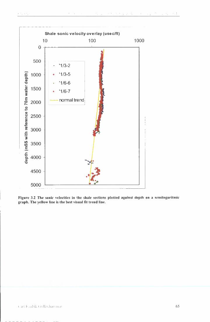
Shale sonic velocity overlay (usec/ft)
10 100
0
500
£ 1000 Q. 0) -o S 1500 5
| 2000 o +->
| 2500
2 3000
% 3500 B
f . 4000 "D
4500
5000
1000
- '1/3-2
• '1/3-5
• '1/6-6
• '1/6-7
- normal trend
Figure 3.2 The sonic velocities in the shale sections plotted against depth on a semilogaritmic graph. The yellow line is the best visual fit trend line.
I a i ! P r t i i n k C i v l l e n n a m i r u i r 65

Chapter 3 Comparison o f different pore pressure methods using a North Sea wel l .
N 1/6-7
pressure (MPa)
10 20 30 40 50 60 70 80 90 100 500
mud pressure
pore pressure 1000
original sonic pore pressure
1500 a RFT
Overburden 2000
CD hydrostatic
2500
3000
3500
4000
4500
5000
Figure 3.3 A comparison of the calculated pore pressure from the d'exponent (blue dots) and the sonic velocity calculated pore pressure.
The critical assumptions with such a method is that it is based on a uniform lithology.
The mudstone must have a constant volume of clay versus quartz i f one single normal
compaction trend is to be used (Aplin et al., 1995). Secondly the only source of the
over pressure is assumed coming from disequilibrium compaction (Swarbrick, 2002).
Carl Fredrik Gyllenhammar (56

Chapter 3 Comparison o f different pore pressure methods usiny a North Sea well .
3.2.2.1 Tertiary
The initial pore pressure interpretation based on drilling parameters suggested that the
excess pore pressure began at approximately 1000 meters. The sonic data suggests
that this depth could be lowered to 1300 meters. The depth is difficult to detect
without the wireline logs as the 20" casing was placed at lOOOmRKB and the MW
subsequently increased from seawater gravity to 10 ppg. The pore pressure probably
exceeded the mudweight in an interval starting at 1800m, which corresponds with
large cavings observed and sampled on the shaker screens. From 2500 meters and
downwards, no changes in the pore pressure gradient were observed based on the
drilling parameters. The sonic log that was run after having drilled the section
suggested a decrease in the pore pressure gradient.
Generally in the Tertiary section the final pore pressure interpretation was based on
the sonic log rather than the drilling parameters.
3.2.2.2 Chalk
Pressure data in the Chalk were mostly interpreted from RFT and DST measurements
from offset wells. This was later confirmed when the RFT data from the nearest offset
well Nor 1/6-6 became available. Again the mudweight used gives the maximum pore
pressure gradient assuming parts of the chalk have some permeability. At 3534 m, 4
barrels of mud were lost into the formation and the mudweight was lowered from 13.5
ppg to 12.3 ppg. This did not result in increased total gas in the mud, which could
indicate a lower pore pressure than mudweight (i.e. drilling overbalanced), or
alternatively the permeability of the Chalk is too low to allow bleeding of formation
fluid into the borehole (drilling underbalanced in tight formation).
3.2.2.3 Jurassic
The d'exponent was as quite spiky in the Jurassic shale section, and the trend line was
shifted several times while drilling (Figure 3.1). Figure 3.1 only display one of the
many trend-lines paralleling the green line. It was only in retrospect that the one
single alternative trend line (the red line in Figure 3.1) was applied. That d'exponent
derived pore pressure evaluation compares well with the sonic calculated pore
pressure with respect to the pressure transition at 4400 meters. The two methods give
similar results down to 4600 meters. From that depth downwards the sonic velocity
Carl Fredrik Gyllenhainmar 67

Chapter 3 Comparison o f different pore pressure methods using a North Sea well .
increases suggesting rapid reduction of the porosity hence decreasing pore pressure
gradient as well. This is not in agreement with what was observed at the well site. It
was therefore decided to disregard the sonic values and use the drilling parameters for
the final pore pressure evaluation in the Jurassic section.
The following is a description of how the total gas reading was used to interpret the
pore pressure. The rig had top-drive, so the well was drilled with stands, not singles.
This meant that it was 30 metres between each connection not 10. The pumps were
therefore turned off every 10 metres to simulate connections (dummy connections).
When the connection gas (CG) was 10 % higher than total gas (TG), the mudweight
was increased. Drilling was stopped each time new mud was circulated. The well took
a water kick at 4878m and was shut in after a 2.5 bbl of formation fluid had flowed
into the well (recorded as gain in the drilling mud pit). Further down in this sandstone
section a loss circulation situation occurred and loss circulation material circulated to
seal of the permeable sandstone. An RFT log later confirmed this estimate of the
overpressure.
The well operator was quite convinced that the pore pressure gradient increased
continuously while drilling this section with no decreases except through the
sandstone at 4878 meters where the overpressure was constant. The wellsite
evaluation by the author was therefore assumed correct. The well operator was faced
with the following problem: either believe in the empirical drilling data, or deduce an
alternative interpretation of lower pore pressures provided by the wireline data in
particular the sonic log. In particular the sonic log is very powerful in the sense that it
can be correlated from well to well, and is a standard tool to determine shale porosity.
The drilling parameter such as the d'exponent is a function not only of the formation,
but also the drill bit and the drilling mud as well.
The above reveals a weakness in the provision of traditional porosity based pore
pressure prediction using the sonic log data. Additional information on porosity from
the neutron density cross plot suggests that the composition of the mudrocks vary,
which would lead to errors on account of selecting a single normal compaction curve
for the pore pressure evaluation. It is also suggested that the origin of the pore
pressure in this area has several sources (Bjorlykke, 1996, Holm, 1996, Gaarstroom et
al., 1993), and that consequently these methods do not take them all into account
Carl Fredrik Gyllenhammar 68

Chapter 3 Comparison o f different pore pressure methods using a North Sea well .
With respect to the d'exponent, one has to ask what the initial calibration was based on. The total gas response? Then what decided the total gas response values to be used before the mudweight was increased? What does the maximum mudweight used in the low permeable mudrock section represent? Do the cavings come from differential stress release zones rather than initiated by overpressure in the mudrock? What is the origin of the gas monitored in the drilling fluid while drilling through the mudrock and how is it related to the pore pressure? This is very empirical indeed. But never the less this method is universal with respect to the cause of the overpressure. It is purely based on observations and the actual mud weight that was used to drill these formations.
The following is the well operator's comment in 1992: "It is interesting to note that
the sonic log often indicates normal compaction or much lower overpressure than
what is seen from the RFT results in the interbedded sandstones of Jurassic age. This
problem is not discussed any further in this report".
This will be discussed later in this chapter.
3.3 Normal Compaction in the North Sea.
Hansen (1996) developed a normal compaction curve for the North Sea using shale
velocity from several exploration wells in the Norwegian sector of the North Sea. The
equation was an Athy type equation (2.1.3.1);
at = 191xe0 0 0 O 2 7 x d e p , h [E3.3]
The Hansen curve was based on three exploration wells; Nor-8/3-2, Nor-9/2-2 from
the Central North Sea and Nor-30/2-1 from the Northern North Sea. It was assumed
that the shales in these wells were to a large degree dewatered and had hydrostatic
pore pressure. These wells are located in an area with low geothermal gradient
relative to the axial rift portion of the North Sea basin.
Carl Fredrik Gyllenhammar 69

Chapter 3 C omparison of different pore pressure methods using a North Sea well.
Figure 3.4 show the Hansen dataset compared wi th the dataset in this study. At 2000
meters the shale slowness span from 160 jxsec/ft to 90 |i,sec/ft. The distance from Nor-
1/6-7 to Nor-9/2-2 is less than 100 km. It shows that it is diff icul t to define a normal
Shale sonic velocity overlay (usec/ft)
500
30/2-1
normal (rend
Normal trend (Hansen.1996)
4000
1000
Shale sonic velocity overlay (usec/ft)
60 80 100 120 140 160 180 200
'30/2-1
4000
lormal trend
- Normal trend (Hansen.1996)
Figure 3.4 Shale velocities from the wells in Figure 3.2 compared with the wells used by Hansen (1996). The Figure to the left has a logarithmic X-axis. At such a plot the Athy type normal compaction trend become a straight line. O n the plot to the right it is much more obvious that the well used in this study are different from the one used by Hansen (1996).
compaction trend applicable to these two datasets. Ideally, the normal compaction
trend for mudrocks should be defined f rom a continuously subsiding basin in which
the compaction o f the sediments had been going on for such a long time that all
excess pore f lu id have migrated out o f the system and the pore pressure has reduced
to hydrostatic. In the case o f any upl i f t and erosion, the eroded succession must have
been reburied by an equal amount o f overburden. Ideally porosities should come from
core measurements, rather than calculated from wireline logs.
For more than 32 years the Ocean Dri l l ing Program (ODP) and its predecessor Deep
Sea Dri l l ing Project (DSDP) have explored the history o f the ocean basins and the
nature o f the sediments and the crust beneath the ocean floor. Uti l izing the dri l l ships
Joides Resolution and Glomar Challenger rocks and sediments have been recovered
from beneath the sea floor at more than 1000 locations (sites) worldwide. The density
Carl Fredrik Gyllenhammar 70
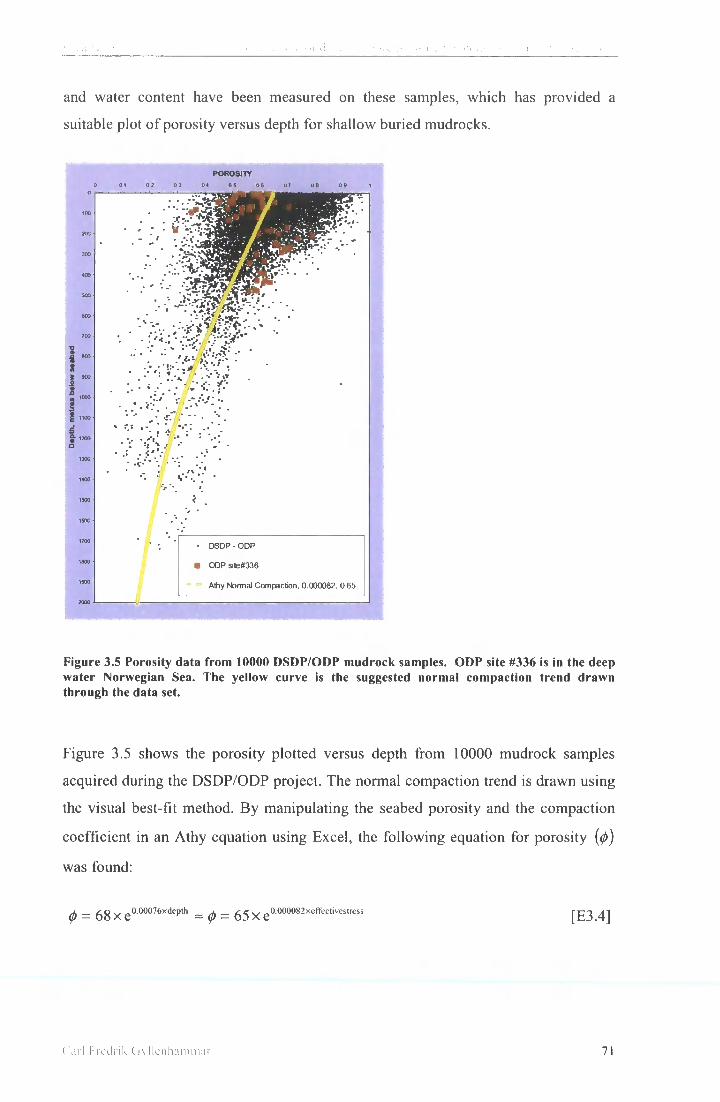
and water content have been measured on these samples, which has provided a
suitable plot o f porosity versus depth for shallow buried mudrocks.
POROSITY 0.4 05 0.6 07 0.8 0.9
I I | | 1100
i ,
DSDP - ODP OOP site#336 Athy Normal Compaction, 0.000082, 0.65
Figure 3.5 Porosity data from 10000 D S D P / O D P mudrock samples. O D P site #336 is in the deep water Norwegian Sea. The yellow curve is the suggested normal compaction trend drawn through the data set.
Figure 3.5 shows the porosity plotted versus depth from 10000 mudrock samples
acquired during the DSDP/ODP project. The normal compaction trend is drawn using
the visual best-fit method. By manipulating the seabed porosity and the compaction
coefficient in an Athy equation using Excel, the following equation for porosity (<p)
was found:
0 = 6 8 x e
0- 0 0 0 7 6* d eP t h ~ (p — 55 x e
0 0 0 0 0 8 2 > < e f f e c t i v e s t r e s s 4 j
Curl I redrik Ciy]lenhamniar 71
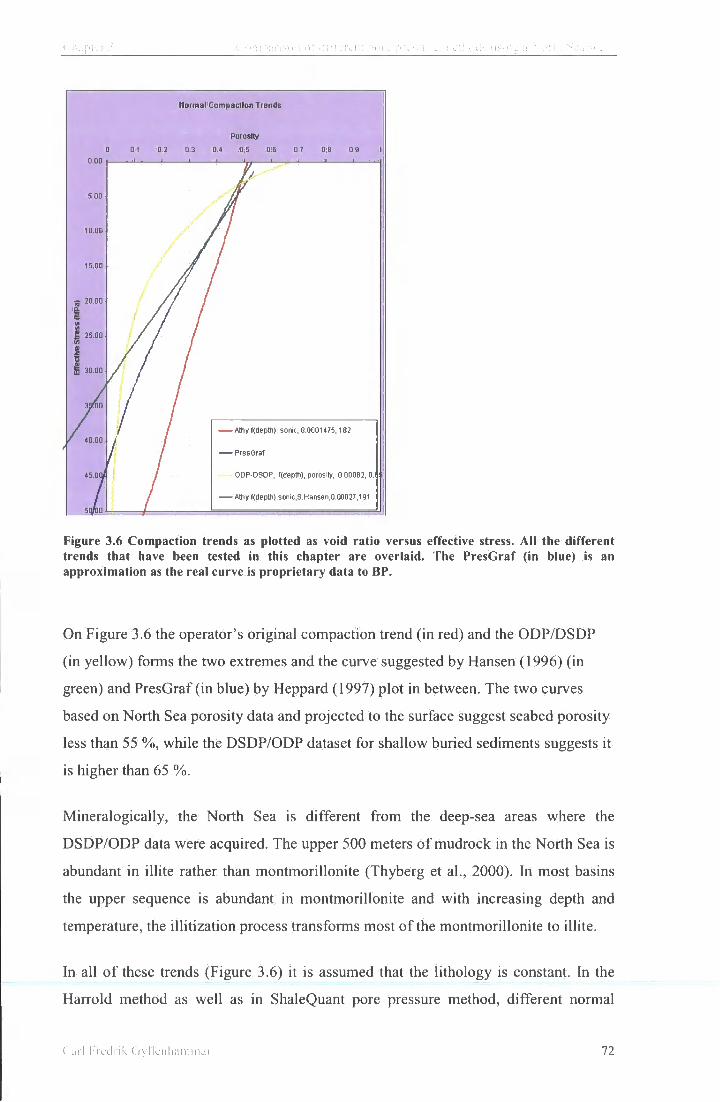
Normal Compaction Trends 1 Porosity
0 0 1 0 2 03 0 4 0 5 0 6 0 7 OS o g
3 0 3
10 JO
! f, 00
>0 !fl ! 2' 30
30.00
/ 10 -1
PresOraf
5 00/
afco
ODP 4: j
Amy f(de
50/001
0.00
Athyf(deptt>), sonic, 0.0001475,182
ODP-DSDP, f(deptfi), porosity, 0.00082, O.I
Athy f(deptti),sortic,S.Hansen,0.0O027,191
Figure 3.6 Compaction trends as plotted as void ratio versus effective stress. Al l the different trends that have been tested in this chapter are overlaid. The PresGraf (in blue) is an approximation as the real curve is proprietary data to B P .
On Figure 3.6 the operator's original compaction trend (in red) and the ODP/DSDP
(in yellow) forms the two extremes and the curve suggested by Hansen (1996) (in
green) and PresGraf ( in blue) by Heppard (1997) plot in between. The two curves
based on North Sea porosity data and projected to the surface suggest seabed porosity
less than 55 %, while the DSDP/ODP dataset for shallow buried sediments suggests it
is higher than 65 %.
Mineralogically, the North Sea is different f rom the deep-sea areas where the
DSDP/ODP data were acquired. The upper 500 meters o f mudrock in the North Sea is
abundant in illite rather than montmorillonite (Thyberg et al., 2000). In most basins
the upper sequence is abundant in montmorillonite and with increasing depth and
temperature, the illitization process transforms most o f the montmorillonite to illite.
In all o f these trends (Figure 3.6) it is assumed that the lithology is constant. In the
Harrold method as well as in ShaleQuant pore pressure method, different normal
l "arl i'rednk Cn llenhanimar 72

Chapter 3 Comparison of dilierent pore pressure meihods using a Nonh Sea weil.
compaction trends for different clay content are used. The problem then arises: what parameter to use to determine the clay content? In the Harrold method wireline logs are used such as the gamma ray. The gamma ray gives clay content as the volume of phyllosilicates versus quartz (Harrold, 1999). The gamma ray is not always a reliable indicator o f shale content due to occasional radioactive material, such as potassium feldspar, in the sandstone (Doveton, 1985). A different method is to use the neutron density cross plot. That method w i l l also approximate to a measure the volume of clay (Vcl) equivalent to the volume o f phyllosilicates. The problem with the neutron density cross plot method is that these logs in most wells only cover the reservoir section, not the overburden. It is not uncommon for these estimates to differ from one another, and the lowest estimate is usually taken (Doveton, 1985). In the case o f Nor-1/6-7 the average Vc l f rom the different methods are 58% from neutron density, 54% from ShaleQuant and 40% from gamma ray. This average is not for mudstone alone, but for the whole succession, including sandstone and chalk. It is therefore not far from the average clay content composition o f 10000 shales reported by Yaalon (1965) as 59%.
Carl Frednk Gyllenhammar 73
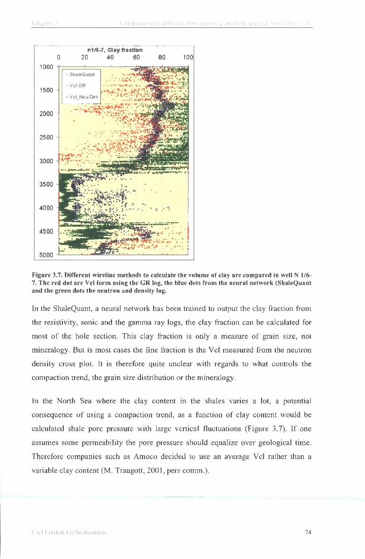
Chapter 3 Comparison of different pure pressure methods using a North Sea .veil
n1/6-7, Clay fraction 0 20 40 60 80 100
1000 I
Sh - P.I iuant
Vc\-GR 1500
Vcl Neu-Den
2000
2500
3000 - * T
3500
4000
4500
5000
Figure 3.7. Different wireline methods to calculate the volume of clay are compared in well N 1/6-7. The red dot are V c l form using the G R log, the blue dots from the neural network (ShaleQuant and the green dots the neutron and density log.
In the ShaleQuant, a neural network has been trained to output the clay fraction f rom
the resistivity, sonic and the gamma ray logs, the clay fraction can be calculated for
most o f the hole section. This clay fraction is only a measure o f grain size, not
mineralogy. But is most cases the fine fraction is the Vc l measured from the neutron
density cross plot. It is therefore quite unclear with regards to what controls the
compaction trend, the grain size distribution or the mineralogy.
In the North Sea where the clay content in the shales varies a lot, a potential
consequence o f using a compaction trend, as a function o f clay content would be
calculated shale pore pressure with large vertical fluctuations (Figure 3.7). I f one
assumes some permeability the pore pressure should equalize over geological time.
Therefore companies such as Amoco decided to use an average Vc l rather than a
variable clay content ( M . Traugott, 2001, pers comm.).
Carl Fredrik Gyllenhammar 74

The two compaction trends, the operator's and the one generated f rom the
DSDP/ODP data set were used later in this chapter while comparing different pore
pressure equations. As the Athy equation used in the operator's calculation was based
on a sonic velocity versus depth, the equation was transferred to porosity versus depth
and to porosity versus mean effective stress. The process was done in Excel by
varying the compaction coefficient and the seabed porosity with the fol lowing
equations as result;
at = i 8 2 x e 0 0 0 0 1 4 7 5 x d e p , h - <j> = 4 8 x e 0 0 0 0 1 3 x d e p , h - </> = 55 x e 0.000025xeffectives tress
e = 2 . 2 - 0 .75x log 1 0 ' t f * * ™ ^ [ E 3 . 5 ]
3.3.1 Palaeocene and Lower Eocene
The Palaeocene to lower Eocene section serves to illustrate how complex and
heterogeneous the mudrock composition is in the North Sea. The Eocene deposits
consists o f up to four hundred meters o f smectite-rich mudstone low in quartz while
the underlying Palaeocene has less smectite, but more chlorite. The overlying
Neogene sediments are rich in il l i te, kaolinite and chlorite (Thyberg et al., 2000).
The high-smectite content in the Palaeocene and Lower Eocene is related to volcanic
activity. This zone is often referred to as the t u f f zone consisting o f water-laid tephras
(Morton and Knox, 1990). Pearson (1990) suggested that sufficient volumes o f
pyroclastics could have been deposited on adjacent landmasses to supply the basin
with smectite-rich sediments. In simple terms the glass in the tephras reacts wi th
water to form smectite and silica (Wensaas et al., 1989). In well Nor-30/2-1 the t u f f
zone is estimated to be 76 meters thick, out o f which 16 meters was cored (1952m -
1968m). 168 individual t u f f beds ranging in thickness from a few millimetres to 28
centimetres are identified. They add up to 6.85 meters or 44% of the core. It is
believed that the 76 meter t u f f layer consists o f 500 individual ash beds adding up to a
theoretical ash thickness o f 33 meters after compaction to 1950 meters (Morton and
Knox, 1990). These beds occur over the entire North Sea extending onshore into
Carl Fredrik Gyllenhammar 75
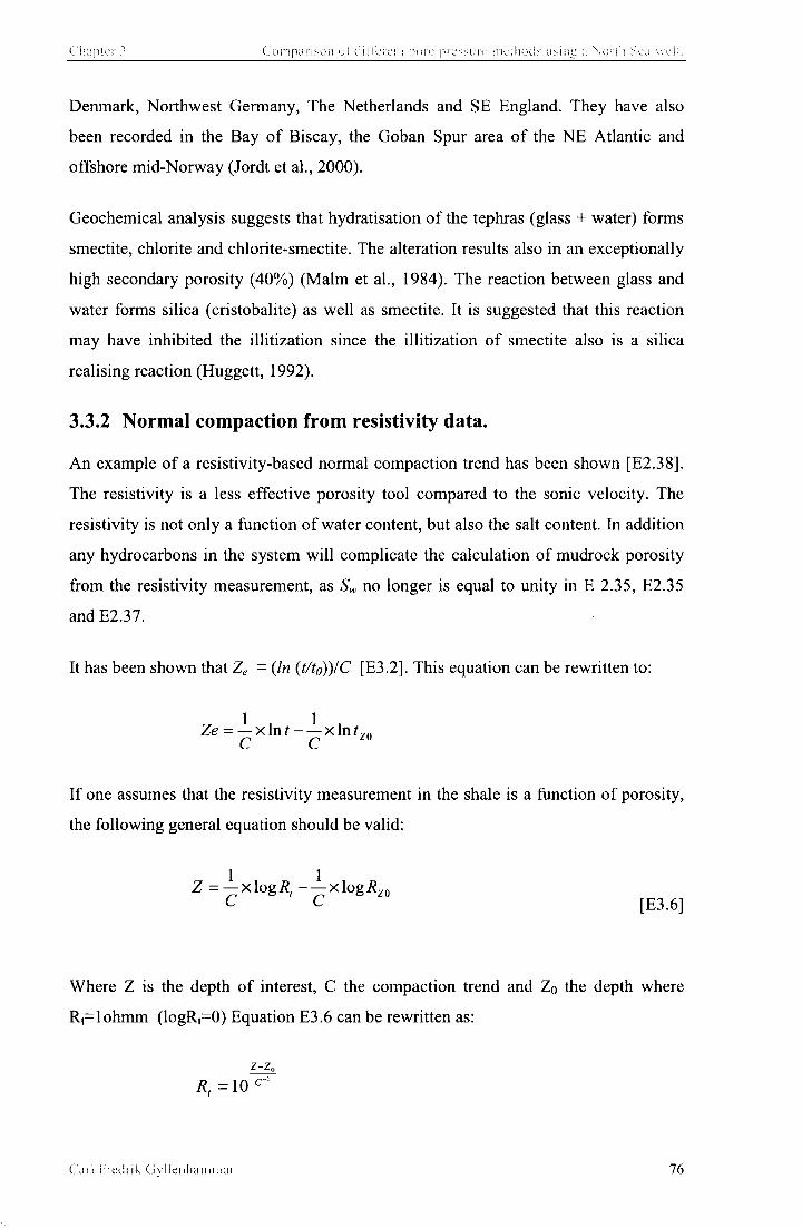
Denmark, Northwest Germany, The Netherlands and SE England. They have also
been recorded in the Bay o f Biscay, the Goban Spur area o f the NE Atlantic and
offshore mid-Norway (Jordt et al., 2000).
Geochemical analysis suggests that hydratisation o f the tephras (glass + water) forms
smectite, chlorite and chlorite-smectite. The alteration results also in an exceptionally
high secondary porosity (40%) (Malm et al., 1984). The reaction between glass and
water forms silica (cristobalite) as well as smectite. It is suggested that this reaction
may have inhibited the illitization since the illitization o f smectite also is a silica
realising reaction (Huggett, 1992).
3.3.2 Normal compaction from resistivity data.
A n example o f a resistivity-based normal compaction trend has been shown [E2.38].
The resistivity is a less effective porosity tool compared to the sonic velocity. The
resistivity is not only a function o f water content, but also the salt content. In addition
any hydrocarbons in the system w i l l complicate the calculation o f mudrock porosity
from the resistivity measurement, as Sw no longer is equal to unity in E 2.35, E2.35
and E2.37.
It has been shown that Ze = (/« {t/t0))IC [E3.2]. This equation can be rewritten to:
1 , 1 , Ze = —x\nt xlnt
C C zo
I f one assumes that the resistivity measurement in the shale is a function of porosity,
the following general equation should be valid:
Z = - J ; X l o g / ? ( - ^ x l o g i ? Z 0
C C [E3.6]
Where Z is the depth o f interest, C the compaction trend and Zo the depth where
R t =lohmm (logR,=0) Equation E3.6 can be rewritten as:
2-Z„
R, =10 c " '
Carl Fredrik Gvllenhammar 76

Chapter 3 Comparison o f different pore pressure methods using ;i North Sea well ,
Macgregor (1965) published resistivity trends f rom 26 different wells f rom the Gulf o f Mexico area (Figure 3.8). A visual average line w i l l be satisfied by equation 3.7 using Zo - 4131.6 and the compaction coefficient C = 9672.2:
Z-4131.6
R, = 10 9 6 7 2 2
Such a reference trend line is a function o f the overburden pressure, temperature
gradient, mineralogy and resistivity o f the pore f luid. Applying the same curve in the
North Sea makes the assumption that all the variables are the same. It is quite obvious
they are not, but for simplicity and curiosity a test was run with the results in the next
chapter.
mmhos
1 a 00-)
i ! H I ! m 11 1 a 00-) j [ Iff
1
I f
I4OO0
I *
I4OO0
-
Figure 3.8 Twenty-six wells in 5 offshore areas and 4 onshore fields (MacGregor, 1965). The pink line is a suggested normal trend for the Gul f of Mexico.
Traugott (1997) suggested improving the use o f the resistivity data by applying a
temperature correction. This results in a shift in the normal compaction trend. A test
was run using EXCEL and where the exponent in the Eaton equation was changed.
[E3.7]
Carl Fredrik Gyllenhammar 77

Chapter :• >. omp.n isun r>i jiMViviu pure pressure method* using a Xorih See: wcM.
This experiment showed there is little to achieve by modifying the exponent in the Eaton equation itself.
As the resistivity is a function o f temperature it is important that is corrected so that
real differences in the resistivity are used in the calculation. Arps (1953) published the
first correction;
RT] R T 2
Tx +21.5°C
T2 +21.5°C [E3.8]
T2 is the reference temperature chosen and is normally set to 100°C.
The Arps (1953) equation was modified by Kern et al. (1977);
r, +22°C + £T RT\ — R
T2 + 2 2 ° c + sr [E3.9]
In sandstone ST is zero and increases as a function o f rising clay content. The
published data suggest a ST as high as 12°C based on their experiments (Kern, 1977).
Wi th the current information it was decided to use equation 3.9 setting ST =0.
Using the temperature-corrected resistivity it was found that a normal trend line using
equation 3.7 with Zo - 3000 and a compaction coefficient C = 4000 would give a
satisfactory result;
2-3000
R = 10 4 0 0 0
i [3.10]
3.4 Wireline log pore pressure calculation
The pore pressure calculation methods have been tested first by using different
equations wi th the same input parameters. This is not simple, as certain methods have
implicit unique input parameters. The fol lowing is a description o f five tests done
using EXCEL spread sheets. The first three tests were based on shale porosity other
than from the resistivity log. The fourth test was on the different compaction trends,
Carl l-redrik Gyllcnhammar 78

Chapter Comparison of"different pore pressure methods usinii a North Sea well
while the last tested the resistivity log as input parameter versus shale porosity f rom
sonic, density and neutron logs.
In the first test, the idea was to evaluate the conventional equivalent effective stress
method (E2.17) wi th an Athy type compaction trend (E2.19) versus the University o f
Durham method developed by Harrold (1999) with its unique equivalent effective
stress method (E2.19). The compaction trend used for equivalent depth method has an
Athy type compaction trend (E3.5) while the University o f Durham method has a soil
mechanical type compaction trend (E2.20). The parameters used in E2.20 were 2 for
void ratio (=67 % porosity) at 100 KPa (=about 10 meters below sea floor) and 0.65
as the compaction coefficient C. This was done to make the equation 2.20 track the
equation 3.5 as closely as possible.
Well 1/6-7 Pore Pressure, GR>50API Pressure (MPa)
0.00 10.00 20.00 30.00 40.00 50.00 60.00 70.00 80.00 90.00 100.00 110.00 0 1 1 1 1 1 1 ' — •
Overburden
F ' J Hydrostatic
Fracture pressure )0fl
University of Durham
Equiv.Depth, Athy, 0.000025, 0.55
Conoco pore pressure
Mud Weight
SOiiij
i ro
Figure 3.9 Pore pressure in mega-Pascal versus depth in meters. The green solid line is the overburden and the blue solid line is the hydrostatic pressure. The equivalent depth method calculated pressure is in blue dots while the orange is the University of Durham method. The dashed black curve is the operator's interpretation while the olive solid line is the mud weight. The red crosses are the R F T direct pore pressure measurements.
Figure 3.9 shows the comparison o f the two methods, the University o f Durham in
orange crosses and the equivalent depth in blue dots. Both o f the calculations suggest
Carl Fredrik Gyllenhammar 79
Chapter 3 Comparison of dilleicnt pore pressure methods using :i North Sea well.
pressure lower than the hydrostatic pressure above 1000 meters. This is unreasonable and can be a result o f low porosity mudrock below the sea floor. It can also be a mudrock with unusually high matrix velocity. This w i l l be further discussed in the next chapter. Below the chalk (from 4380 meters) the pressure transition zone is better defined by the University o f Durham method than the equivalent depth method. However, below 4650 meters both methods fai l to properly identify the continuing increase in the pore pressure gradient down to the Jurassic sand at 4878 meters.
The Durham University equation was developed using data f rom Southeast Asia wells
and yields a higher pressure than lithostatic f rom 1700 to 1900 meters. It is likely that
this equation is area dependent, and needs local calibration. In the Tertiary section, the
equivalent method gave a reasonable result, but below the Chalk in the Jurassic
section both methods failed.
In the second test (Figure 3.10), the equivalent effective stress method (blue dots) was
tested against the Eaton method (red dots) using the sonic log and the same Athy type
compaction trend (E3.5). The input parameter to the Eaton method was the sonic
velocity while the shale porosity is used in the equivalent effective stress method. In
the shallow section, the Eaton method also suggests pressures lower than the
hydrostatic, but only just below. The possible high-pressure gradient described f rom
wellsite at 1850 meters based on abundant caving was only picked up by the
equivalent effective stress method. Below the Chalk in the Jurassic, the Eaton method
calculates initially higher and more realistic pressures. Then the sonic velocity
increases from 4650 meters down to 4878 meters. The porosity calculated f rom the
density neutron log does not vary as much as the sonic does in the Jurassic shales.
This suggests that the shale velocity is more influenced by changing matrix velocity
than the water content, hence the porosity. The Eaton method suggests a drop in
pressure from 85 MPa at 4650 meters to below 60 MPa while the equivalent effective
stress method drops from 72 MPa to 64 MPa. The pressure in the sand at 4878 meters
is lOOMPa. So both methods are wrong, but the large negative variation is reduced by
using porosity rather than the sonic velocity.
This is illustrated in the third test (Figure 3.11) where the equivalent depth method
(solid blue) using the sonic log is compared with the Eaton method (red dots). The
equivalent depth method suggests more variability in the Tertiary section than the
Carl l-redrik Gyllenhammar 80
Chapter 3 Comparison ot'dili'ereni pore pressure methods using a North Sea well.
Eaton method. In particular the interval from 1800 to 1900 m was characterised by abundant cavings, suggesting pore pressure above the mud weight (solid olive). The calculated shale pore pressure in the Jurassic is about the same.
Based on these three tests it appears that the equivalent effective stress method, as
described in Chapter 2.2.1.1, is the method, which gives the best results in the
Tertiary section. The equivalent effective stress method is preferred since it is based
on physical principles rather than empirical relationships. The input parameter should
also be the calculated shale porosity rather than a single log measurement such as the
sonic velocity.
The fourth test (Figure 3.12) examines different compaction trends using the
equivalent effective stress method with the porosity as input. The pore pressure using
the DSDP/ODP normal compaction trend (E3.4) suggests considerably higher
pressures than were calculated by the operator in the Tertiary section. The sediments
just below the seafloor become sub-hydrostatic wi th this compaction trend, but only
down to 500 meters, not to 1000 meters. The calculated pressure is not higher than the
mud weight and therefore not unreasonable. In the Jurassic, it is the only model that
predicts the pressure transition zone and calculates the magnitude o f pore pressure
down to 4650 meters. Figure 3.12 shows that the sonic velocity (green solid line)
increases f rom 140 |isec/ft to 90 |isec/ft at 5000 meters. Using the Hansen (1996)
sonic to porosity transform, it suggests that the porosity decreases f rom 40 to 13 %
(not on Figure 3.13). The porosity calculated by combining the neutron and density
logs (Figure 3.13 and 3.14, red solid line to the right) suggests a decrease f rom 30 to
20 %.
This reduction in porosity results in a calculated pore pressure much lower than
suggested by the drilling parameters. One may say that all these arguments are
circular arguments. Unfortunately there are no direct pore pressure measurements
possible in the shale. But one would expect that the shale pressure close to the sand at
4878 meters would have a pore pressure close to the sand pressure. On the other hand,
what kind o f evidence is there for the assumed correlation between the shale porosity
and the pore pressure? It is possible that we are observing the maximum loading that
Carl Fredrik Gyllenhammar 81

Chapter 3 C omparison of different pore pressure methods using a North Sea weii.
particular shale have experienced and that it now have been pressurized by lateral transfer via the underlying sandstone, (J. I l i f fe (2003), pers. comm.).
On Figure 3.14, the sonic log suggests a sharp transition zone where the velocity
decreases f rom 100 usec/ft at 4870 to 120 (isec/ft at 4878 meters. Even with the
DSDP/ODP trend, the shale pressure using the equivalent method is suggested to be
10 MPa lower than in the sand. That is a 10% error i f one assumes that the first few
centimetres o f the shale have the same overpressure as the underlying sandstone. The
porosity increasing towards the shale-sand intersection suggests that f lu id is forced
from the sand into the shale. What we do not know is the actual shale pore pressure.
Well 1/6-7 Pore Pressure, GR>50API Pressure (MPa)
0.00 10.00 20.00 30.00 40.00 50.00 60.00 7000 80.00 90.00 100.00 110.00
Overburden
ECO Hydrostatic
Fracture pressure iriKi
Equrv. Depth, Athy, 0.000025. 0.55 1=00
2rC:C + R.F.T
Mud Weight
Eaton sonic >Cuu
jcrjfj
Figure 3.10 Pore pressure in mega-Pascal versus depth in meters. The green solid line is the overburden and the blue solid line is the hydrostatic pressure. The Eaton equation with the sonic log as input (red dots) compared with the Equivalent depth method with the porosity as input (blue dots). The red crosses are the R F T direct pore pressure measurements. The values are listed in Appendix 2.
Carl Fredrik Gyllenhammar 82

Chapter Comparison ot different pore pressure methods using a North Sea well.
Well 1/6-7 Pore Pressure, GR>50API Pressure (MPa)
0.00 10.00 20.00 30.00 40.00 50.00 60.00 70.00 80.00 90.00 100.00 110.00 o +- 1 1 1 1 1 1 ' 1 1 1 1
Overburden
Hydrostatic
Fracture pressure
2CCI
N , Mud Weight
Eaton sonic
Equivatent depth Sonic SXiu
- ( I ,
1CC0
Figure 3.11 Pore pressure in mega-Pascal versus depth in meters. The green solid line is the overburden and the blue solid line is the hydrostatic pressure. The Eaton equation in red dots compared with the Equivalent depth method in solid blue, both with the sonic log as input. The red crosses are the R F T direct pore pressure measurements. The values are listed in Appendix 2.
Well 1/6-7 Pore Pressure, GR>50API Pressure (MPa)
0.00 10.00 20.00 30.00 40.00 50.00 60.00 7Q00 80.00 90.00 100.00 110.00
Overburden
3CC Hydrostatic
Fracture pressure 1000 Equiv.Depth. Athy. 0.0001475, 0.48
Equiv.Depth, Athy,0.0076, 0.68 <5C
Conoco pore pressure
to + Ft.F.T
Mud Weight k - i J
<o :
<: o
4300
Figure 3.12 Pore pressure in mega-Pascal versus depth in meters. The green solid line is the overburden and the blue solid line is the hydrostatic pressure. The Equivalent depth method tested with two different normal trends. The Athy equation used by the operator of well Nor-1/6-7 (blue dots) versus the D S D P - O D P based trend (red dots).The red crosses are the R F T direct pore pressure measurements. The values are listed in Appendix 2.
Car l Fredr ik ( i \ l l e n h a m m a r 83

V\HI1(6-7 Pore ftessuB, GR>9ttOP1
Rwstrefl^ Sonic values in usec/ft Porosity 40.00 moo eaoo moo aooo aioo xaai 11000 12000 ISQOO W O O 5GO WOO too 2000 2500 3000 S O D * K
Increasing sonic velocity •
g«XJ
- J "5
Decreasing sonic velocity
Oerhiden m o FractuefTessue
Bw.Dedn.ArK 0000032, 066 Ecpv Cejih Alty. 0000025, Q66 Quoco p re ocGais 4 ' I I
+ RF.T.
Figure 3.13 The shale porosity (red solid curve to the right) and the shale travel time (green solid line to the right) versus depth in the Jurassic section. The x axis is in % for porosity, (isec/ft for the sonic log. The curves to the left of the overburden (strait solid green line) is in MPa. Between the overburden and the hydrostatic pressure (left most solid blue) are from left the pore pressure calculated using the sonic log as input (blue curve) then with porosity as input (orange curve). The values are listed in Appendix 2.
v\8l 1/6-7 Pore Pressure, GR>5&aPI Sonic values in usec/n Porosity FfcesstrefvPa)
V I ' I I ' d 'X t • • „ . . . 17.00 19 00 21 00 23.00 25
) CAmuden C Ffadure [ressure • BMV.Q(*./ttiy,QOXJ082 0.65 &MV.D-rth, Atly. QCDXJ25 Q55 CtnXD porecressiffi
RF.T.
S i t
(XI 1 1 I ) Sonic log
I K B Kick at 4878 mR
i
1 •si ! !
Figure 3.14 Figure 3.13, the pressure transition zone from 4850- 4890 meters. The values are listed in Appendix 2.
Car! Frcdrik Civllenhammar 84

Chapter 3 Comparison of different pore pressure methods using a North Sea well.
Well 1«-7 Pore Pressure, GR>50API Pressure (MPa)
0 00 10.00 20.00 30 00 40.00 50.00 60.00 7000 80.00 90.00 100.00 110.00 0 t ' ' ' 1 1 1 1 1 '
Overburden
51 Hydrostatic
,0f Fracture pressure
151
2C« Mud Weight
; 5f • Eaton resislivrty
Eaton sonic 5005
J5u
50C '
Figure 3.15 Pore pressure in mega-Pascal versus depth in meters. The green solid line is the overburden and the blue solid line is the hydrostatic pressure. The Eaton equation with the resistivity log as input (green dots) compared with the Eaton sonic (red dots). The red crosses are the R F T direct pore pressure measurements. The values are listed in Appendix 2.
In the last test, the two Eaton methods were tested; based on sonic as input versus
resistivity as input. In the resistivity model, the resistivity data were temperature
corrected as suggested in Chapter 3.3.1. The normal trend was developed using
equation 3.10. It is important to recall the PCA test in Chapter 2.2.4, which suggests
that the resistivity in this well is a pore porosity indicator.
In the Tertiary section, the resistivity-derived pressure is influenced by the low salt
content in the brine. The compaction trend is based on a constant salt content
appearing f rom about 1500 meters. From 1500 meters the two Eaton methods have
comparable results down to 2500 meters. Down to the top Chalk, the resistivity-
derived pressure is considerably higher than the sonic-derived pore pressure
estimation, but below the mud weight used. In the Jurassic section the resistivity
model is the only wireline method that suggests a continuous increase in pressure with
depth down to the Jurassic sand at 4878 meters. This could be explained by salt water
being forced into the low porosity mudrock f rom the underlying overpressured
Carl Fredrik Gyllenhammar 85

Chapter 3 Comparison of diilereni pore pressure methods using a North Sea well .
sandstone, which would increase the resistivity and lead to higher overpressure in the
pore pressure estimation. But there are other concerns with using the resistivity.
Firstly, it is very difficult to compare the normal compaction trend versus other
porosity trends. There is no one simple way of calculating the porosity from the
resistivity log. A bigger concern is when hydrocarbons are present. Hydrocarbons will
increase the resistivity and therefore decrease the calculated pore pressure.
3.5 Comparing the North Sea with the Gulf of Mexico Basin
The objective of this study using the Gulf of Mexico was to compare a standard
wireline pressure model with a 3-D basin model. The wireline pressure model is not a
1-D model, but rather a model where the effective stress in the shale is assumed to be
a function of the shale porosity (calculated from the sonic velocity or the resistivity)
and the overburden stress. This is calculated for each point in the section independent
of any other calculated pore pressure. The study area is a classic Gulf of Mexico
(GoM) mini-basin (Figure 3.16). In a study such as this, it was important to preserve
confidentiality. As earlier practice within the GeoPOP group, the well name was
invented, and the name "Vimto" was used as the code-name for this Gulf of Mexico
oilfield. The two Vimto wells were provided to the GeoPOP research group along
with the seismic data to do a case study.
The basin has received rapid, deep-water sedimentation since the beginning of the
Miocene. Mobile salt covered the area in early Miocene times. Subsequent salt
movement resulted in diapiric rise and salt withdrawal. The basin is close to the outer
shelf/upper slope break, with water depth in the range of 400 meters. The sediments
consist of turbidite sands interbedded with mudrock. Due to extreme rates of
deposition and low temperature gradient (20°C/km), it is likely that disequilibrium
compaction is the primary overpressure generating mechanism (Yardley and Couples,
2000).
For the 1-D model it was decided to use the PresGraf model (Chapter 2.2.2.2) with the
default normal compaction trend. That particular model has proved to give good
Carl l-redrik Civllenhammar 86

t t t i i l K'. - l > ! I
results in most of the Gulf of Mexico, (M. Traugott ,2000, pers comm). As the
GeoPOP project was near its end it was important to complete this analysis rather
quickly.
G. Yardley at the Heriot-Watt University did the basin modelling using the PetroMod
3-D versions 6.0/6.1 software. The basin modelling software is based on a grid
system. The grid nodes can only move vertically. This makes it difficult to model salt
movements. In effect salt was treated as a facies within each layer and assumed
deposited along with muds and sands. The permeability in the sand was set to a
constant of 100 mDarcy, which in effect is instantaneous free flow over basin scale.
The mudstone permeability is shown on Figure 3.17. The normal compaction used
was derived from ShaleQuant (Chapter 2.2.3) and is shown on Figure 3.18.
i m
Figure 3.16 Depiction of salt features in the area around the basin. The local depocenteres are termed mini-basins (Yardley and Couples, 2000).
Carl Fredrik Gyllenhammav 87

Chapter 3 Comparison o f different pore pressure methods using a North Sea wel l .
3.6 Vimto#l and #2
The two wells were drilled from the same location and deviated from about 8000 ft.
The available data consisted of wireline and MWD (or LWD) data. The operator
experienced logging problems resulting in sections where wireline logging was
impossible. MWD logs were then spliced in. There appears also to have been
problems with the calibration of the GR tool between the different hole sections.
Since the wells are so close, most of the pore pressure calculations were preformed on
the Vimto #2 well. The pore pressure was calculated using three methods. Two
methods where the sonic log were used as the input for the Eaton method and the
Equivalent Depth Method of determining pore pressure. The third method was the
Eaton method using the resistivity log as input. A l l of the calculations used an
overburden curve based on integrating the density log from the wells. The normal
compaction trend used is a curve that is proprietary to BP-Amoco and available while
using their software PresGraf. The Eaton method based on the resistivity log was also
tested with a log linear normal compaction curve.
Car! Fredt ik Gyllenhammur 88
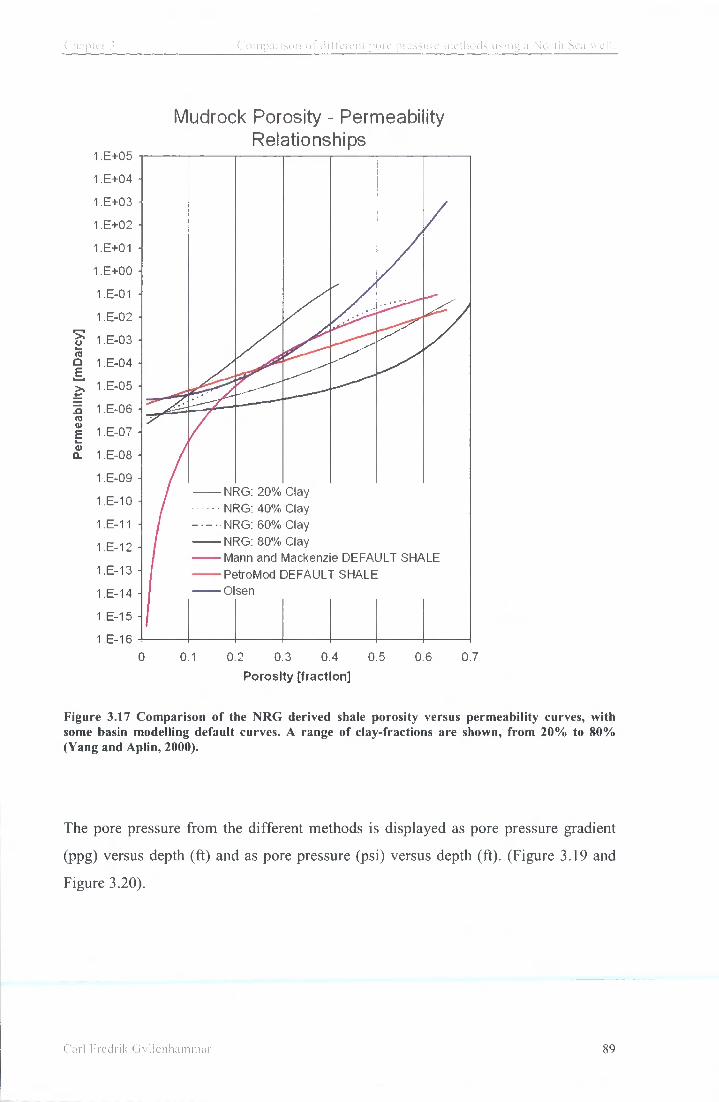
Chapter 3 Comparison o f different pore pressure methods using a North Sea w
1.E+05
1.E+04
Mudrock Porosity - Permeability Relationships
1.E+03 -
1.E+02 •
1.E+01
1 .E+00
1.E-01 -
1 .E-02
1 E-03
1.E-04
1.E-05
1.E-06 -
1.E-07 •
1.E-08
1.E-09 -
E-10
.E-11
1.E-12 -
1.E-13
1.E-14
1.E-15
1.E-16
• NRG: 20% Clay NRG: 40% Clay NRG: 60% Clay NRG: 80% Clay Mann and Mackenzie DEFAULT SHALE PetroMod DEFAULT SHALE Olsen
0.1 0.2 0.3 0.4
Porosity [fraction]
0.5 0.6 0.7
Figure 3.17 Comparison of the NRG derived shale porosity versus permeability curves, with some basin modelling default curves. A range of clay-fractions are shown, from 20% to 80% (Yang and Aplin, 2000).
The pore pressure from the different methods is displayed as pore pressure gradient
(ppg) versus depth (ft) and as pore pressure (psi) versus depth (ft). (Figure 3.19 and
Figure 3.20).
Carl Fredrik Gyllenhammar 89
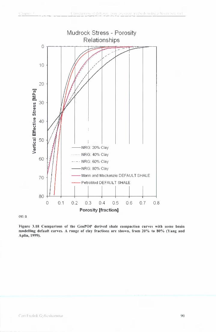
Chapter 3 Comparison o f different pore pressure methods using a North Sea well .
Mudrock Stress - Porosity Relationships
o
10
20
I w 30 V)
i f )
> 40 4>
« 50
1 NRG: 20% Clay
NRG: 40% Clay
60 NRG: 60% Clay
NRG: 8 0 % Clay
Mann and Mackenzie DEFAOLT SHALE 70
PetroMod DEFAULT SHALE
SO 0 0.1 0.2 0.3 0.4 0.5 0.6 0.7 0.8
Porosity [fraction] on a
Figure 3.18 Comparison of the GeoPOP derived shale compaction curves with some basin modelling default curves. A range of clay fractions are shown, from 20% to 80% (Yang and Aplin, 1999).
Carl Fredrik Gyllenhammar 90

Chapter 3 Comparison o f different pore pressure methods using a North Sea well.
feet Vimto2
Vimto2 .D43 Vimto2 .D46 Vimto2 .Mdt
10000
12000
14000
16000
i mm
2000-̂
8OOO1
10000
12000
14000
16000
4000 8000 12000 Pressure, psig 2000/div
16000 0 120 200 50 GR Acoustic
Figure 3.19 Pore pressure prediction for Vimto #2. The blue curve is the pore pressure calculated using the Eaton method and the shale sonic velocity as input. The red line is pore pressure using the equivalent depth method. The pink diamonds are the MDT pressure points. The red line to the left is the overburden. The values are listed in Appendix 3.
Vimto #2, MDT
10000 10250 105O0 12760
Pressure (psr)
10750 11000 11250 11500 11750 12000 12250 125O0 12750
I3250
I350O
3750
. inn
I4250
I4500
4750
15000
• MDT
~ ~ " Shale PP Eaton, sonic
Figure 3.20 The reservoir section for well Vimto#2. The MDT pressures are generally 50 to 100 psi higher than the calculated shale pressures.
Carl Frednk Gyllenhammar 91

Chapter 3
Vimto Results: 2D Modelled Pressures Lateral Transfer: Complete Salt 0
• Est imated Water Pressures 1000
Hydrostatic
2000 Li thostatc
2D Model led Pore Pressure 3000 Deep Sands
4000
5000
6000
7000 CO n 8000
9000
or 10000
1000
12000
13000
14000 \
15000 -
16000 -
17000 -0 10 20 30 40 50 60 70 80 90 100
Pressure [MPa]
Figure 3.21 The red curve is the pore pressure calculated from a 2-D model alowing for lateral transfere (Yardley and Couples, 2000).
The pore pressure evaluation using the sonic data in these two wells appears to be not
very sensitive to the method applied with regard to the equivalent depth method or the
Eaton method (Figure 3.19). This suggests that the pore pressure generated in these
two wells is predominantly generated by disequilibrium compaction. Figure 3.20
shows that the MDT pressures are 50 to 100 psi higher than the calculated pore
pressure in the shales. The difference between the model results and the MDT data is
\ •
Carl Fredrik Gyllenhammar 92

Chapter 3 Comparison o f differeni pore pressure nielhods using a Nonh Sea wel l .
1% and must be considered a very good result. The results from the 2-D basin modelling yields equally good results (Figure 3.21).
Basin modelling packages determine pore pressure with depth by calculating the fluid
loss through a sequence of sedimentary layers during burial. Fluid loss is assumed to
follow the Darcy flow theory. One of the problems is that the porosity-permeability
relationships are based on empirical observations from high porosity samples, (Mark.
Osborne (2001) pers comm). In principal, calculation of pore pressure in three
dimensions has the potential to accurately model pore pressure as the model accounts
for lateral flow within the system. This is not the case in a one-dimensional model
using wireline logs from one well. The shortcoming is the resolution and the lack of
geological control between the wells data points needed for such a calculation. Any
extensive low permeability layer will radically change the fluid flow regime. The
model would possibly gain from using pore pressure calculated from wireline logs as
input to the basin model.
3.7 Summary and conclusions
The single most important factor with respect to calculating pore pressure is the
selection of the appropriate normal compaction curve. The mudrock porosity is
important and it is suggested to combine as many porosity logs as possible. An
analogy can be made with seismic processing where noise is suppressed by stacking
as many traces as possible.
Concerning the equation to calculate the pore pressure, there is no reason not to use
the equivalent effective stress method as long as it is assumed that most of the
overpressure is generated by disequilibrium compaction. Some have argued that it is
important to use mean effective stress and not vertical effective stress to calculate the
overburden.
An other concern is using the equivalent mean effective stress method in place of the
traditional equivalent depth method. The argument is that the variation of density with
depth wil l result in an inaccurate pressure unless the calculation is referred to mean
effective stress (Chapter 2.2.1.1.).
Carl Fredrik Gyllenhammar 93
Chapter 3 Comparison oi J i Herein pore pressure methods using a North Sea wel l .
The resistivity log shows promising results in the North Sea Jurassic section, but there is no good scientific explanation for its ability to yield a good pore pressure prediction. The PCA analysis in Chapter 2.2.4 suggests no correlation between porosity and resistivity in that particular well. The correlation between the pore pressure and resistivity could be coincidental and could be a function of hydrocarbons in the shale.
In the Jurassic shales in the North Sea, the challenge is to first calculate the porosity,
then relate the calculated porosity to pore pressure. This study has clearly shown that
large differences exist between sonic and neutron-density derived porosities. The low
porosity suggests low pore pressure while the drilling parameters as well as the pore
pressure in the porous reservoir suggests high pore pressure.
It is also suggested by some authors that the excess pore pressure in the Central North
Sea has several sources (other than disequilibrium compaction) that these prediction
methods do not take into account (Bjorlykke, 1996, Holm, 1996, Gaarstroom et al.,
1993). These other causes would include chemical compaction such as illitization,
hydrocarbon generation and lateral transfer.
In the last exercise, the Vimto case study in the Gulf of Mexico, three different
methods were used to calculate the pressure: Eaton, PresGraf and the equivalent depth
combining shale velocity with the PresGraf normal trend (Figure 3.6). A list of the
calculated pressures can be found in Appendix 1. At shallow depths, the difference is
much larger than in deeper stratigraphic intervals. The reason is the low gradient of
the compaction curve at shallow depth shown seen in Figure 2.5. At 1000 meters the
pressure difference is 13%. That difference decreases with depth and is less than 5%
at 2000 meters. At 4000 meters the difference is less than 1%. At that depth the
PresGraf normal trend crosses the DSDP/ODP trend (Figure 3.6). Calculation of the
pore pressure at that depth using the Equivalent Depth Method, and only changing the
compaction trend from the PresGraf trend to the trend used by the operator of well
Nor 1/6-7 (Equation 3.5), drops the calculated pressure by 28%. The actual shale
pressure that fits the MDT data in the Vimto area is in the range of 9900psi (68MPa)
at 4000 meters. Shifting the compaction trend to the initial trend used in North Sea
drops the calculated pressure to 7600psi (52MPa).
Carl hredrik Gyllenhammar 94

Chapter 3 Comparison of different pore pressure methods using a North Sea wel l .
In conclusion, I suggest that when calculating pore pressure it is important to
eliminate all errors. This means that to calculate the pressure in shales generated by
compaction the best method is the equivalent mean effective stress method. As input
parameter it is recommended not to use a single wireline log but the best calculated
porosity. Having said this, the difference at 4000 meters wil l be in the range of 0-2
MPa. By changing the compaction trend the shift can be up to 15MPa. This is clearly
significant. I want to end with Eaton's (1975) statement again; "the methods used to
establish normal trends vary as much as the number of people who do it". His 27
years-old statement is still valid today.
Carl Fredrik Gyllenhammar 95

Chapter 4 The impact of the Glaciat ion on ibe Normal compaction in the North Sea
Chapter 4 The impact of the Glaciation on the Normal compaction in the North Sea.
Carl Fredrik Gyllenhammar 96

Chapter 4 The impact of"the Glaciat ion on the Normal compaction in the North Sen
4.1 Introduction
A comparison of normal compaction porosity profiles from the North Sea versus the
Gulf of Mexico reveals a marked difference in the upper 500 meters of sediments.
The most striking difference is the porosity of the mudrocks, which may be related to
the glacial history affecting Northern Europe and which would not have affected the
Gulf of Mexico, south of the Pleistocene glaciation.
The Recent offshore glacial history of the Central North Sea has received little
investigation in comparison with the older rocks whose sedimentary and tectonic
evolution related to the Eocene and older oil and gas fields (Riis and Fjeldskaar,
1992). Consequently the thickness, character and internal architecture of the glacial
sedimentary packages in the North Sea have not been well explored. Further, the
impact on burial and fluid flow processes episodic of glacial loading and removal of
load have not been fully assessed.
NW Europe is currently responding to the lithospheric rebound from the removal of
the Weichselian / Devensian ice sheet, but Berger and Loutre (1999) suggest there
have been nine or ten major cycles of ice sheet build up (glacial period) followed by
melting (interglacial period) during the last one million years (Figure 4.1). The extent
of successive ice sheets is known from onshore data to vary. The sedimentary record
of each is found mainly in glacial deposits, dominantly tills. Unravelling the history of
each cycle onshore is made difficult by repeated cannibalisation of the earlier
sedimentary record during successive ice movement and associated scouring. The
offshore record is not well documented, in part because of a lack of data in the
interval between shallow boreholes (typically 200m) drilled for site investigation and
near-surface sedimentary research, and deep boreholes (> 1000m to 5000m) drilled for
oil and gas. Bad borehole conditions also reduce the quality of shallow wireline logs.
Carl Fredrik Gyllenhammar 97

Oxygen isotope ratio (d) 5.5 5 4.5 4 3.5
0.0 -I '•• — 1 ' = = i a
0 :
Glacial J 6
Interglaciai Oxygen isotope ralio (d)
10
1 5
10 Periods of
rapid transition
C 1
Figure 4.1 A curve showing the variation in oxygen isotope composition of the sea-water for the last 6 million years. The oxygen isotope data are based on foraminifera from three boreholes near the coast of Ecuador (Shackleton et al., 1990; Shackleton et al., 1995.
98

Chapter 4 The impact of the Giaeia i ion on the Normai compaction in live North Sea
4.2 Glacial history
As the last ice age, the Weichselian / Devensian (Wisconsin in the North America),
has removed most of the traces of its precursor, only assumptions can be made about
the older ones. The geological record of older glaciations is often sporadic. It begins
with poor and fragmentary evidence from Archean rocks followed by a long
Mesoproterozoic non-glacial period (2.0 - 1.0 Ga). The Late Proterozoic (1.0 Ga to
just before the Cambrian) glaciogenic deposits are known from all the continents.
They provide evidence of one of the most widespread and long-ranging glaciations on
Earth. Most regions display evidence of several glaciations separated by warmer
periods. In Phanerozoic times glaciations are reported from Ordovician in Africa,
possibly Brazil and Arabia. Silurian and Devonian glaciations are limited to South
America. The most significant Phanerozoic glaciation took place in the Permo-
Carboniferous, between 350 and 250 Ma, across a large area of the Gondwanian
supercontinent (protocontinent). There is no direct geologic record of Mesozoic
glaciations but small ice sheets can have developed at high latitudes. Late Tertiary
glaciations are recorded from Antarctica about at 36 Ma.
Ice began to accumulate on Antarctica 20 million years ago. Glaciations in the
Northern Hemisphere were initiated at about 6 Ma (Eyles and Young, 1994). Oxygen
isotope data from ODP leg 104 Site 642B and 644A suggest intensification of the
glaciation periods from 2.75 Ma and a new intensification from 1 Ma (Jansen and
Sjoeholm, 1991). This data suggest an important change in the climate from a stable
to a cyclic changing climate, causing of periods of glaciation and interglaciation.
During the last 1 million years it appears that the Earth has been changing from one
equilibrium to the other, being cold (glaciated) or warm (such as today). At first the
cycle was 41,000 years in length, but from 900,000 years ago the glaciations have
been more intense with thicker ice sheets, but less frequent, down to 100 000 year
cycles. These cycles correlate with the astronomical theory, which is most associated
with Milutin Milankovitch (1879-1958) (Williams et al., 1998). In sum, one
superimposes several variables concerning the Earth orbit around the sun. The three
most important are the obliquity of the Earth's axis to the plane of the ecliptic cycles,
the eccentricity of the orbit and the precession. But the Milankovitch (1941) theory
does not explain the dramatic change from a stable to a cyclical climate. The
Carl Fredrik Gyllenhammar 99

n a p t e r -I I'hc impact of the Glaciat ion on ;he Normal compaction in the North Sea
intensification of glaciations also correlates with an increase in the number and
thickness of volcanic ash layers (Prueher and Rea, 1998). It is obvious that one cannot
assign one prime cause to drive the changes as long as the cyclic situation to day has
only taken place over the last 1 million years. Plate tectonic movements are believed
to drive the most dramatic climatic changes over geologic time.
The extent of the last big ice sheet, the Weichselian / Devensian (in Europe), has been
assessed by studying enclosed depressions on land and linear incisions on the
continental shelf (Ehlers and Wingfield, 1991). The enclosed depressions are about 6
km wide, 30 km long and 400 meter deep, often occupied by lakes orthogonal to the
ice margins. They do not go beyond the ice and coincide with the distribution of tills.
The offshore depressions divert from the onshore in that they appear not to coincide
with tills. These observations have been used as an argument to suggest that offshore
incisions are not formed by glacial activity. The lack of identification of tills could be
due to limited core samples, lack of wireline log interpretation or attributed to erosion
during the post-glacial transgression. But the ongoing debate during the last decade
following the increased knowledge from the North Sea has led to a continuous
reduction of the extent of the last ice age. Despite this it is suggested that an extensive
glaciation began after 29,400 years and lasted until 22,000 years (Sejrup et al., 1994).
The ice sheet extent of northern Eurasia covered most of Ireland, most of England,
Scotland, Shetland, most of the North Sea, most of Scandinavia, the Barents Sea,
Spitsbergen, Balticum and East Russia (Hughes, 1998; Svensen et al, 1999) (Figure
4.2). The maximum Wisconsin ice sheet thickness in the North-America was more
than 4000 meters and the maximum Weichselian / Devensian ice sheet thickness over
Fennoscandia exceeded 2000 meters. The average thickness of the Weichselian /
Devensian ice sheet was about 1600 meters (Pollard and Thompsom, 1997). 1,600
metre has been suggested as the maximum thickness of a Weichselian / Devensian ice
sheet over the North Sea with its crest from Southwest Norway to Scotland (Figure
4.2).
During the Weichselian / Devensian glaciation, Holland remained ice-free. But
Holland had been covered by ice sheets during previous glaciations. It is also well
known that the Weichselian / Devensian glaciation was far from being the most
extensive glaciation in the Alps (Hughes, 1998). Earlier Quaternary glaciations were
Carl hredi ik Gyllenhainmar 100
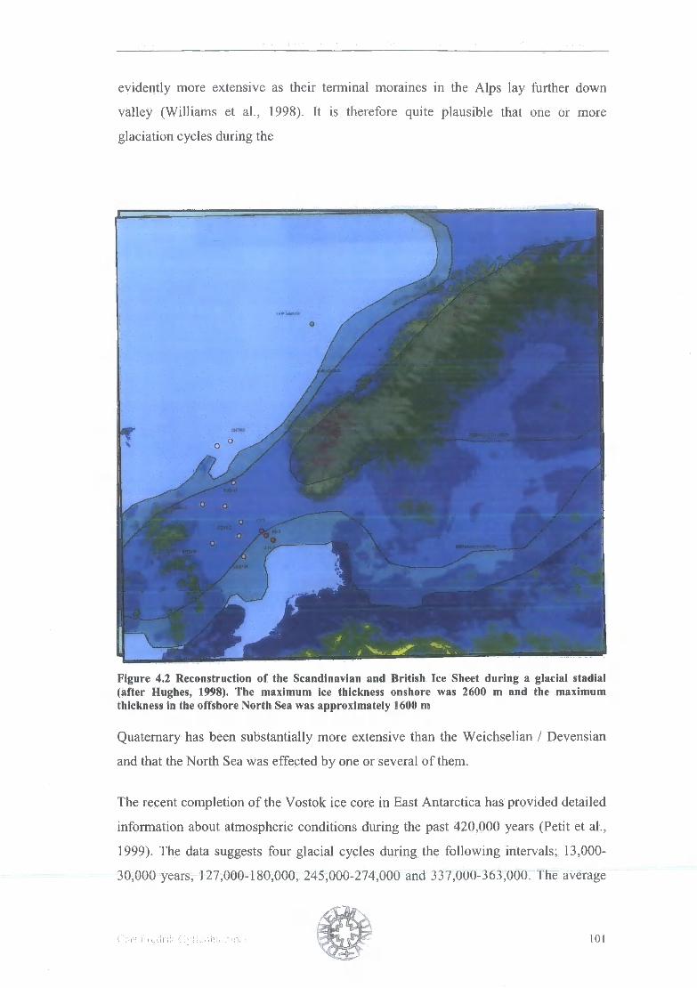
evidently more extensive as their terminal moraines in the Alps lay further down
valley (Williams et al., 1998). It is therefore quite plausible that one or more
glaciation cycles during the
Figure 4.2 Reconstruction of the Scandinavian and British Ice Sheet during a glacial stadial (after Hughes, 1998). The maximum ice thickness onshore was 2600 m and the maximum thickness in the offshore North Sea was approximately 1600 m
Quaternary has been substantially more extensive than the Weichselian / Devensian
and that the North Sea was effected by one or several of them.
The recent completion of the Vostok ice core in East Antarctica has provided detailed
information about atmospheric conditions during the past 420,000 years (Petit et al.,
1999). The data suggests four glacial cycles during the following intervals; 13,000-
30,000 years, 127,000-180,000, 245,000-274,000 and 337,000-363,000. The average
(';•! ! !• n.on!< Cn ikniv.ir.iiii; i 101

( ' hap ie r 4 T h e i m p a c i o f the C i l ac imion on the N o r m a i c o m p a c t i o n in I he \ o n l i htu.
duration is 30,000 years for these glaciations, and a total of 125,000 years over the last 420,000 years.
4.2.1 The Neogene - Pleistogene sedimentary succession
In the Viking Graben the basin subsided rapidly in Late Oligocene-Early Miocene
times (Dahl and Augustson, 1993). The Mid-Miocene unconformity is a result of
period of uplift and erosion, which followed at this time. This tectonic event is
concomitant with the Alpine Orogeny. During the Pliocene and Pleistocene period, a
massive delta system prograded westward associated with Baltic rivers from the
Fennoscandian Shield and on the south margin deltas associated with northern
German river systems (Cameron et al., 1993). The sediments consist mostly of low
permeable mudstone interbedded with sands. These fluvio-deltaic deposits reach up to
1,400 metres in the Central Graben and filled most of the southern North Sea Basin.
The system was later peneplaned and following minor erosion, the Late Quaternary
sediments rest upon the unconformity (Dahl and Augustson, 1993).
There is a clear separation of depositional style between the Early and Middle
Pleistocene deposition. The older underlying deltaic sediments were deposited under
relatively stable climatic and sea level conditions (Scourse et al., 1998). In contrast
the younger overlying non-deltaic division, though volumetrically less significant,
were deposited during the high amplitude climatic and sea level oscillations
characteristic of Quaternary glacial deposits in the North Sea. The thickness of the
Quaternary succession is often difficult to access due to limited well data. In the
shallow cores used in this study the Quaternary succession is generally 50 to 60
meters. Based on seismic interpretation associated with the well data, the Quaternary
section is assumed to be as much as 600 m in the U.K. sector of the North Sea
(Stacker et al., 1985).
Late Pleistocene ice-scoured surfaces were first identified in the Central North Sea
from regional seismic profiles (Stoker and Long, 1984). Numerous 3-D seismic
surveys in the North Sea have made it possible to explain unresolved features on the
earlier 2-D seismic within the Quaternary succession. Azimuth maps from the 3D-
seismic data cube have revealed lineated surfaces interpreted to be subglacial features
in the Norwegian Channel (Lygren et al., 1997). On Haltenbanken buried ice-scours
Car l F redr ik G y l l e n h a m i n a i 102

Chapter 4 The impact o f the G h i c i a t i o n on the N o r m a l c o m p a c t i o n in the N o r t h Sea
are similarly interpreted from time-slices within the Upper Pliocene sequences (Long
and Praeg, 1997).
4 . 3 Tills
Depositional processes refer to the mechanisms that lay down the final deposit.
Glacial, fluvial, gravitational and aeolian processes are involved. Of these, only
glacial deposition is unique to the glacial environment. Primary deposits, laid down
uniquely by glacial agents are TILLS. Tills have been transported and deposited by or
from glacier ice, with little or no sorting by water (Dreimanis, 1989). In the glacial
environment active depositional centres shift position on a daily, seasonal and random
basis. The glacier will advance and retreat so the sedimentary deposits are subject to
deformation, reworking and resedimentation (Dreimanis, 1989). Sub-water tills are
therefore unlikely to be primary deposits. There are different types of tills and the two
most important in this case are melt-out tills, which refers to direct sediment
deposition through melting of stagnant or very slowly moving debris-rich ice and
lodgement tills which are generated byplastering of glacial debris from the base of a
sliding glacier on to the underlying rocks. The destruction of pre-existing structures
under very high cumulative strains makes tills difficult to identify.
Sediments deposited in glacial environments (tills) commonly have much lower
density and porosity than sediments deposited in pure marine environment
(Dreimanis, 1989). Sediment grain size is highly variable. For example, large
boulders have been encountered several hundred metres below seabed inbedded in
mudstone in the offshore mid-Norway.
Hence i f we were to search for offshore tills we would either use shallow cores or
wireline logs. And we would be searching for unusually low porosity (high density)
sediments in the shallow section in areas where no or limited uplift and erosion has
taken place.
Car l F redr ik G y l l e n h a m m a r 103

Chnpie r 4 [ lie impac t o f the G lac ta t ion on the N o r m a l c o m p a c t i o n in (he N o r t h Sea
4 . 4 Mudrock porosities
The British Geological Survey has collected core samples from 576 sites in the
offshore area of the British Islands, mostly for palynological studies. At several sites
in the North Sea the density and water content of the sediments were measured. The
wells reached a total depth below seabed ranging from only a few meters to 1228.5
m). These porosity data were compared with the DSDP/ODP data (Figure 3.4 and
Figure 4.3). A l l the DSDP/ODP sites are located in deep water where there has not
been any ice loading. The general trend of the porosities in the shallow succession
from borehole data can therefore be used to compare with the DSDP/ODP data.
Anomalously low porosities would traditionally be interpreted as possible unloading
in shallow basins such as the North Sea
In addition to the Central North Sea wells, porosities from shallow cores were also
available from the Statfjord Field, Troll Field (Andersen et al., 1995) and
Haltenbanken. The shallow core from the Troll field was 40 meter deep in 358 meters
of water (Andersen et al., 1995). The lower part of the core consists of sediments from
the Norwegian Trench Formation and the measurements of water content and density
suggests they are over-consolidated. The overlying Kleppe Senior Formation is
normally consolidated and has been deposited during the last 15,000 years after the
last ice sheet melted (Andersen et al., 1995).
The database used for this study was compiled using direct porosity measurements
from 100 DSDP/ODP sites, 9 BGS sites and wireline data from 13 exploration wells
(Figure 4.2 and Table 4.1). The DSDP/ODP porosities are a collection of about
40,000 porosity data points from 100 different sites around the world (ODP internet
WEB site, 2002).
Figure 4.3 show the porosities plotted vs. depth with reference to the seabed rather
than sea surface. While the DSDP/ODP densities of the first few meters of sediments
below the seafloor range from 50 to 80 %, the North Sea data range from 30 to 50 %.
This low porosity trend continues through the upper 500 - 600 meters of sediments in
the North Sea. Below that depth the porosity trend steps up by 20 % and joins the
expected normal trend based on DSDP/ODP data. Such low porosities in the shallow
sediments have also been reported from the Troll field (Andersen et al., 1995). The
Car! Fiec lnk G y l l e n h a m m a r 104

Chapte r 4 I he impact o f ihe G l a c i a i i o n on ihe N o r m a l c o m p a c t i o n in the N o r t h Sea.
thickness of the Quaternary succession in the central axis of the North Sea has been previously estimated to be up to 600 m (Stoker et al., 1985; Gatliff et al., 1994). Seismic data suggest Pleistocene deposition and erosion with several generations of incisions (Ehlers and Wingfield, 1991). These low porosity sediments are therefore assumed young sediments (Pliocene and Quaternary). It is generally assumed that there was no tectonic movement in the North Sea during Pliocene and Quaternary (i.e. no uplift and erosion is evident) and the only alternative explanation is related to glacial loading and unloading.
The low porosity data suggest that the sequences are not a result of sediment supply
distally from the glacial activity. I f so the porosities would have been closer to the
DSDP/ODP normal trend, hence higher. The base of the glacial sediments and
interglacial sediments is taken as the depth where muddy sediments return abruptly to
the "normal compaction curve" defined from North Sea as well as by the ODP/DSDP
mudrock data. The North Sea tills are sub-water tills that have undergone reworking
by non-glacial processes such as sea bottom currents. The core samples may therefore
be very different from the primary tills seen in onshore exposures.
Table 4-1 BGS sits and exploration wells.
BGS sits Exploration wells
BH7702 BH8119 1/3-5 2/7-15 6507/2-1 6507/10-1
BH7703 BH8134 1/5-2 2/11-7 6507/3-1
BH8117 BH8137 1/6-7 6506/11-2 6507/7-1
BH8118 2/4-9x 6506/12-4 6507/8-5
C a r l F redr ik G y l l e n h a m m a r 105

( hapler -i The impac t o f the G l a c i a t i o n on the N o r m a l c o m p a c t i o n in the N o r t h Sea.
POROSITY 0 0.1 0 2 0.3 0.4 0.5 0.6 0.7 0.8 0.9 1
200
t o :
^*>Jrl
! :
7N
HO J
:
iluO
i,;u;;
r i u i
DSOP-ODP
• ODP site#336
* British Geobbgical Survey, shalow cores
• Platform Site shalow cores :....(-
1?6-7 N
• Haltenbanken data
. Ml
Figure 4.3 Porosity versus depth. A compilation of core measurements and wireline calculated porosities.
4 . 5 Oxygen isotope data
Oxygen isotope data provide evidence for the volume of water locked up in
continental ice sheets (Shackleton and Opdyke, 1973). Oxygen occurs in two
common, stable isotopes, 1 6 0 and 1 8 0 , of which l 6 0 is the most abundant. The ratio of
these two isotopes in water is temperature-dependent and follows predictable
geographic trends in the oceans, atmosphere, and glaciers. When seawater evaporates,
the heavier isotope O is left behind in remaining seawater, while the resulting water
vapour is depleted in l g O. The oxygen-isotope composition of a water sample is
C a r l T r e d r i k G y l l e n h a m m a r 106

Chapter 4 The impac t ot the G l a c i a t i o n cm the N o r m a l c o m p a c t i o n in the N o r t h Sea
expressed in delta (5) units per mil (l%o = 0.1%) of relative concentrations with
respect to the ratio of standard mean ocean water (SMOW).
1 8 0 / l 6 0 sample - SMOW
5 = X 1000 [E4.1]
SMOW
By definition, 8 is zero for standard mean ocean water. A value of 5 = -10 thus means
the sample has an 1 8 0 / 1 6 0 ratio 10%o (or 1%) less than SMOW.
Each oxygen isotope cycle is characterized by an upward trend from low to high delta
units (8), reflecting an increase in the global ice volume (Figure 4.1) (Shackleton and
Opdyke, 1973; Dawson, 1992). Under present conditions, the volume of land ice is
relatively small, and this ice has 8 values around -30. During glacial periods, however,
isotopically lighter water is removed from oceans and stored in glaciers on land. This
causes slight enrichment of 1 8 0 in sea water to about 8 = +1.5, while glacier ice has
even lower 8 values of around -40. The oxygen-isotope values during past glaciations
are preserved in glacier ice and in fossils buried on the sea floor. These isotopic
records are primarily a measure of changing volume of glacier ice, but the oxygen-
isotope ratios are also affected by temperature, for example, the water temperature.
The long-term record of oxygen isotopes in the Greenland Ice Sheet extends back
more than 250,000 years and the Vostok ice core from Antarctica extends back
420,000 years. These data correlate with fossil data from the DSDP and ODP wells,
which has enabled establishment of the oxygen-isotope ratio curve to get much older
than the base of the oldest ice core. The curve in Figure 4.1 has therefore been
estimated based on study of foraminifera from three boreholes from the coast of
Ecuador (Shackleton et al., 1990; Shackleton et al., 1995; Shackleton and Pisias,
1985).
Dependant on what 8 value one chooses to be the minimum for a glacial episode, the
oxygen isotope data show there have been at least 6 major glacial times with 8 above
4.7. On Figure 4.1, glacial episodes are suggested beginning at 8 = 4.5 with possibly
Car l I r edr ik G y l l e n h a m m a r 107
Chapter 4 The impac t ul"the G l a c i a t i o n on the N o r m a l c o m p a c t i o n in the N o r t h Sea.
more than 9 glacial and interglacial cycles. Continental ice build up reduced the
world's water volume by 5.5% resulting in a sea level drop of 100 to 150 meters with
reference to present sea level (Figure 4.6). Evidence from coral reefs indicates that the
global sea levels have risen, on average, by a 120 m since the last glacial maximum
(Fairbanks, 1989). The fall in sea level was sufficient to remove the sea cover from
the North Sea. As the ice sheet build-up continued, the dried-up sea bottom of the
previous North Sea became covered under up to 1500 meters of ice.
It is important to take into account the uncertainties in these studies. The amount of
water or ice required for analysis is small (5-10 g), and stable isotopes can be
measured quite accurately using mass spectrographic techniques. Dating the ice core
is not straightforward. The atmospheric air circulates through the ice long after
snowfall accumulates at the surface. This circulation ceases once the pore spaces are
no longer connected with each other. The age difference between enclosed air and
surrounding ice varies between 2500 years for interglacials and 4300 years for the
coldest intervals (Wilson et al., 2000).
4.6 Time series frequency analysis (CycloLog)
Five exploration wells in the North Sea with gamma-ray logs from near the seafloor to
1000 meters were used to create a correlation of glacial events and to compare them
with oxygen isotope data. The five wells were drilled in the southern part of the
Norwegian sector of the Central North Sea. The distance from Norwegian well Nor-
1/3-2 to Nor-2/11-7 is about 100 km (Figure 4.2). Wireline logs like the gamma-ray
from the shallow section do not show enough distinctive signature to permit
correlation between the wells. This is because these shallow sediments in the North
Sea are generally soft and tend to wash out as they are being drilled. Hence the ability
to recognize glacial cycles has been impossible previously based solely on gamma ray
signature. Most cyclic phenomena such as the oxygen isotope data vary in the time
domain, and are analysed using time series analysis. Wireline log data are always
measured in the depth domain. But the depth axis of any log is a function of
geological time in sequences, where they are not faulted or overturned. Consequently
most logs are a natural expression of a time series of geological variations. But there
Carl Fredrik Gyllenhammar 108

Chapte r 4 The impac t ot the G l a c i a t i o n on the N o r m a l c o m p a c t i o n in the N o r t h Sea.
are important differences between logs and time series. Variations in sedimentation
rates, different compaction trends and
1/3-2 v. 1 t
in
in
\ •
116 -
•
II
3 li1
IM
II
Figure 4.4 To the left is the oxygen isotope data shown in Figure 4.1. To the right is the GR log followed by the Altered G R log from well Nor-1/3-2. The third curve is picks representing sudden changes in the cyclicity of the filtered GR curve. The third curve show peaks, positive or negative representing sudden transitions from high to low G R value, shown as a negative peak (to the left). The opposite results in a positive peak. The last curve is the integration of previous curve. These curve were output from C Y C L O L O G * . This curve represents the cumulative difference between the predicted log values and the actual log values. Breaks in the cyclicity succession may be related to missing sections or abrupt changes in sedimentation rates. A large positive peak could be a condensed section.
discontinuities caused by erosional breaks and periods of non-deposition result in a
non-linear and discontinuous representation of time. Ager (1973) even considers the
gaps to be more important than the sedimentary record. The lithological successions
are possibly a sum of catastrophic events in between long periods of non-deposition.
Carl Fredrik Gyllenhammar 109

Chapter 4 The impact o f the G lac t a t i on on the N o r m a l c o m p a c t i o n in the N o r t h Sea.
Since the glacial events are cyclic events, the idea has been to analyse gamma-ray logs in such a way that any cyclic pattern becomes easily recognizable. The fundamental model for cyclicity is that of the sine wave which sketches out the operation of a circular process as it develops through time. I f it had been a seismic signal an autocorrelation would have given the predominant frequencies in the signal. The problem we are faced with is that two cycles in a wireline log that should had the same frequency in the time domain because it happed during the same time interval have different frequencies because the thickness of the sedimentary succession they cause are different. So an autocorrelation would cancel real signals out as i f it were all noise. The first step in frequency analysis of wireline logs is to remove some noise in a somewhat blind manner compared to what would have been done to a seismic wave. In this case the gamma-ray has generally a ragged and complex character in the high-frequency range. This is because of the somewhat stochastic nature of the gamma-ray measurement. A simple low-pass filter such as a moving average will remove the high frequency spikes. This is illustrated in Figure 4.4. The moving average equation wil l also make the sharp transitions from sand to shale become a rather smooth transition. A median filter calculates the median value of all points within a predefined window and plots the results as a single point at the mid-point of the window. The final result is a smoothed and blocked curve. The filtered curve must now be analysed for the predominate frequencies by analysing small segments at a time. The predominant frequency in that window is then moved up the section and as the cyclicity model breaks down, the break is noted and the section above is analysed. A new set of wavelengths is selected and moved up section til l it breaks down again.
This type of processing can be done using software programs such as CycloLog. The
input data in CycloLog can be the raw gamma-ray wireline log. A median filter with a
l m window filtered the raw gamma-ray log. A best-fit cyclicity model was
constructed for a small widow and the program quantifies the deviation of the filtered
gamma-ray log from the best-fit cyclicity model. A sudden transition from high to low
gamma-ray value is shown as a negative peak and the opposite results in a positive
peak. This is shown on Figure 4.4 as curve number three from the left. This happens
each time the cyclicity model break down and a new set of wavelengths are found. A
large positive peak could be a condensed section. The last step was the integration of
Carl Fredrik Gyllenhammar 110
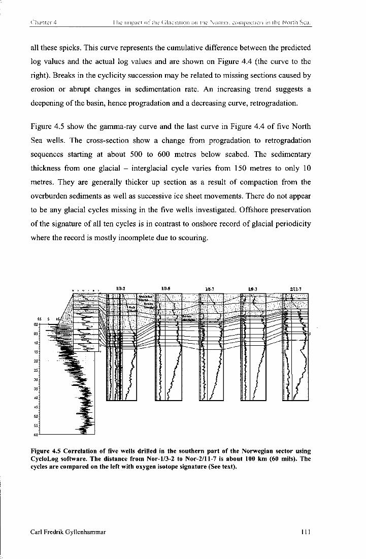
Chapter 4 I he impac t o f lire G l a c i a u o n on the N o r m a l c o m p a c t i o n in the N o r t h Sea.
all these spicks. This curve represents the cumulative difference between the predicted
log values and the actual log values and are shown on Figure 4.4 (the curve to the
right). Breaks in the cyclicity succession may be related to missing sections caused by
erosion or abrupt changes in sedimentation rate. An increasing trend suggests a
deepening of the basin, hence progradation and a decreasing curve, retrogradation.
Figure 4.5 show the gamma-ray curve and the last curve in Figure 4.4 of five North
Sea wells. The cross-section show a change from progradation to retrogradation
sequences starting at about 500 to 600 metres below seabed. The sedimentary
thickness from one glacial - interglacial cycle varies from 150 metres to only 10
metres. They are generally thicker up section as a result of compaction from the
overburden sediments as well as successive ice sheet movements. There do not appear
to be any glacial cycles missing in the five wells investigated. Offshore preservation
of the signature of all ten cycles is in contrast to onshore record of glacial periodicity
where the record is mostly incomplete due to scouring.
1/3-2 1/3-5 1/6.7 1/9-3 2/11-7
lit ' 1 i \
L — . . . . . Z»mia j : :< . • "Jr 5 ,\ 7 7 M t b 3 55 •5
QD 05
15
2B 25 1
3fl
I 35
to 15
SB
55
SB
Figure 4.5 Correlation of Ave wells drilled in the southern part of the Norwegian sector using CycloLog software. The distance from Nor-1/3-2 to Nor-2/11-7 is about 100 km (60 mils). The cycles are compared on the left with oxygen isotope signature (See text).
Carl Fredrik Gyllenhammar 111

Chapter 4 The impac t o f the G l a c i a t i o n on the N o r m a l c o m p a c t i o n in the N o r t h Sea.
The correlation between the time data (oxygen isotopes data) and the depth data (gamma-ray log) was carried out assuming that the change seen in the integrated curve at about 500 to 600 meters correlates with 0.96 My on the oxygen isotope curve (Figure 4.4). 0.96 My is the onset of the first interglacial before the first of the last 10 cold glacial periods. The 10 complete cycles (interglacial followed by interglacial) were identified on the integrated wireline logs from all five wells. Each cycle begins with a sharp increase in the integrated curve suggesting a rapid progradation. This is in correspondence with the sharp drop in d value on the oxygen isotope curve suggesting a rapid melt of the glacial ice resulting a rapid sea level rise. On most of the gamma-ray logs an increase can be seen suggesting an increase in the clay content. This is interpreted as the result of a slow increase in the ice volume and corresponding drop in sea level. The integrated curve shows a decreasing trend suggesting regression. As the water depth dropped the sedimentary deposits became sandier, which is reflected in the gamma-ray log as a lower gamma-ray response.
In general the frequency analysis has enhanced the gamma-ray log to enable this
interpretation. We note that in some wells the section identified as glacial deposits has
experienced borehole wash outs resulting in an incorrect low gamma-ray log
response.
4 . 7 Ice loading and pore pressure
The additional overburden pressure from an ice sheet has an impact on the underlying
sediments as well as the lithosphere. The current isostatic rebound from the last
glaciation is well known (Milne, 1999), but the effect on the underlying sediments is
less well known.
The overburden pressure and the hydrostatic pressure will change during glacial
cycles. During an interglacial period, such as today, the overburden pressure and the
hydrostatic pressure in the North Sea are regulated by the sea level. However, during
a typical glaciation phase, water is removed from the global ocean and the sea level
drops. Since the water depth in most of the North Sea is less than 100 meters and the
sea level drop was in excess of 200 meters during a significant portion of the glacial
cycle most of the North Sea would have been exposed as dry land (Figure 4.6). It has
Carl Fredrik Gyllenhammar 112

( haptei 4 I he impact ot the Glae i a t i i t n on the N o r m a l c o m p a c t i o n in the N o r t h Sea
been shown earlier in this chapter that it is likely that the Scandinavian and the British ice sheets covered a large part of the North Sea. At the time when the ice sheet progressed to cover the North Sea it is likely to have progressed over dry land. As the
75*N 7ffN
70 N 7ffN
r B5*N 65"N t
60 N 60 N
5!TN 5ffN V
50 N 50 N 10'W 0* 10 E 20*E 30'E 10'W 0* 10 E 20'E 30*E
Glacial maximum, 25000 years 15000 years
75'N 75'N
70 N ON
) )
f 65'N 65 N
: 00 N 60 N
35°N
50 N 50N 10 W 20'E 30'E 10 E 10 w 0 20 E 30 E 10'E
8000 years Present
Figure 4.6 The four maps above present the palaeo-coastline for each subsequent crustal motion model. It is important to note that large parts of the North Sea were dry land after the last deglaciation, in each case for a period of several 1000 years.
Carl Fredrik Gyllenhammar 113

Chapter 4 The impac t o f the G l a c i a t i o n on the N o r m a l c o m p a c t i o n in the N o r t h Sea.
ice sheet thickens, the overburden pressure increases. During the initial stage of
deglaciation it is not clear i f the North Sea again became dry land prior to flooding. I f
the ice over the North Sea reached a thickness of 1500 m, the overburden pressure and
hydrostatic pressure would have shifted regularly from -0.8MPa to +13MPa (-117psi
to +1900psi) relative to the present pressure field. The pressure due to 80 m of
seawater is 0.8 MPa and 13 MPa is the pressure due to the additional weight of 1500
m of ice.
Pn Hum (HRii FT* uur» (MPa) ia • (XI in if.: 7:1
is
Lithoststii:
Hydrostatic ID Hydro statK
Pore pressure Pore pressure
; •
\ Sandstone l,iL-nj
•-
:• •- 05
\ \ Pore Pressure rareast \ due to ice-loading
S
ixo t ft* i4«£ftid
J
\ X
\ 1 •
Figure 4.7 The figure to the left show a typical pore pressure profile in the North Sea with no seawater just prior to a glaciation. The sand at 2000 meters subcrope to seafloor and has therefore hydrostatic pressure. During glaciation of the North Sea the overburden pressure and the hydrostatic pressure increase with a pressure equivalent to the weight of the ice-sheet. If the sand subcrops under the ice-sheet the pore pressure will also increase in the sand. But if it subcrops outside the ice-sheet, its pore pressure will only vary as much as the sealevel changes.
During the interglacial period such as today the overburden pressure and the hydrostatic pressure are regulated by the sealevel in the North Sea. In the initial stage of glaciation water is removed and sealevel drops. This is followed by an increase in overburden pressure as the ice cover progresses. Then during deglaciation the North Sea becomes ice free, while there is still enough water retained in the big icesheets, such as over Canada, for the North Sea to become dry land again, prior to flooding as shown in the figure to the left.
Carl Fredrik Gyllenhammar 114

Chapter 4 The impact o f the G l a c i u i i o n on the N o r m a l c o m p a c t i o n in the N o r t h Sea.
At the University of South Carolina the ice loading effect on the underlying sediments
has been modelled using a two-dimensional dynamic model called GEOPETII
(Lerche, 1997). Their model suggests that ice loading increases the pore pressure in
the same way as a load of a car is taken up by increased oil pressure on a hydraulic
jack. Such a process assumes that rocks involved behave perfectly elastically; hence i f
there is no fluid gain or loss, the loading and unloading curve are identical (Yardley
and Swarbrick, 2000). It is well known that is not the case. As the pore pressure
increases, fluid will move laterally to the basin margins as a function of the lateral
permeability. In the case of low lateral permeability the pore pressure as well as the
overburden pressure and with it the fracture pressure wil l increase. It is not known i f
the increase of the pressure will be happening instantaneous down the section at the
same time. The different formations wil l have different compressibility, which may
cause a delay in the pore pressure increase in the stiffer rock than in the more
compressible. In the case where a cap rock was rather stiff it is possible that the
fracture pressure will increase over time as the pore pressure increases over time after
the onset of the ice-sheet. But the increased pore pressure in the underlying reservoir
will happen instantaneously. In some cases this could be enough to fracture the cap
rock seal. Both fracturing and fluid dissipation would then reduce the overpressure
and increase the effective stress. I f the process were perfectly synchronized the
effective pressure would remain unchanged initially, then as a function of time and
permeability, sedimentary compaction wil l reduce the porosity and increase the
effective stress.
The glaciation was periodic and the effective stress increased during each glaciation
period. In addition, new sediments were deposited during each deglaciation period
increasing the overburden stress. Due to the irreversible incremental compaction the
increase in pore pressure from ice loading was more dramatic during the first
glaciation period than from the last. The formation water flow in this model is
assumed to have originated from sediment compaction. The melt water from the ice
sheet was omitted in the GEOPETII model (Lerche, 1997).
In Chapter 2, the vertical effective stress, <xv, was defined as the difference between
the lithostatic stress due to the weight of the overburden, Sv, and the pore pressure, Pj
(Terzaghi, 1936). At the surface the overburden is initially at atmospheric pressure
Carl Fredrik Gyllenhammar 115
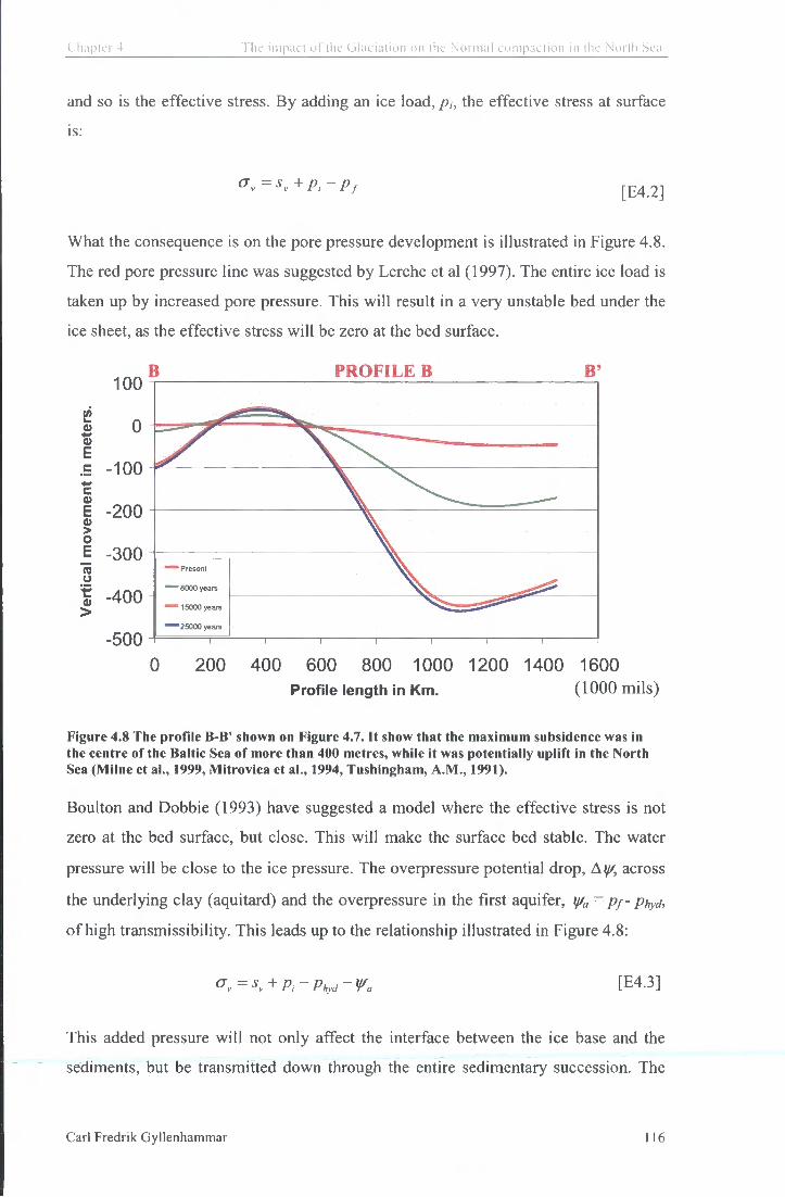
Chapter 4 The impact o f the G l a c i a t i o n o n the N o r m a l c o m p a c t i o n in the N o r t h Sea
and so is the effective stress. By adding an ice load, the effective stress at surface
is:
<rv=sv+Pi - P f [E4.2]
What the consequence is on the pore pressure development is illustrated in Figure 4.8.
The red pore pressure line was suggested by Lerche et al (1997). The entire ice load is
taken up by increased pore pressure. This will result in a very unstable bed under the
ice sheet, as the effective stress will be zero at the bed surface.
0) E c +-» c E 0
P R O F I L E B
TO U t 0)
>
Present
B000 years
15000 years
25000 years
-500 0 200 400 600 800 1000 1200 1400 1600
Profile length in Km. (1000 mils)
Figure 4.8 The profile B-B' shown on Figure 4.7. It show that the maximum subsidence was in the centre of the Baltic Sea of more than 400 metres, while it was potentially uplift in the North Sea (Milne et al., 1999, Mitrovica et al., 1994, Tushingham, A.M., 1991).
Boulton and Dobbie (1993) have suggested a model where the effective stress is not
zero at the bed surface, but close. This wil l make the surface bed stable. The water
pressure will be close to the ice pressure. The overpressure potential drop, A^, across
the underlying clay (aquitard) and the overpressure in the first aquifer, \ f / a - p f - pt,yd,
of high transmissibility. This leads up to the relationship illustrated in Figure 4.8:
Sy + Pi-PHyd-Va [E4.3]
This added pressure will not only affect the interface between the ice base and the
sediments, but be transmitted down through the entire sedimentary succession. The
Carl Fredrik Gyllenhammar 116
Chapter 4 The impact o f the G l a c i a u o n on the N o r m a l c o m p a c t i o n in ihe N o r t h Sea.
pore pressure wil l increase with the ice load in all aquitards and aquifers unless the
permeable layer initially had hydrostatic pressure and communication to seabed
beyond the extent of the ice sheet and the permafrost. It is important to distinguish
between these two cases, when the aquifer has hydrostatic pressure with
communication to seabed and the case where the aquifer has limited extent and is
overpressured. In the first case, there will be an overpressure drop through the
aquitard equal to the overpressure ( y / a ) from the ice load on the surface. The pressure
development becomes very complex as the pressures increase in all previous
overpressured sections, while it remains hydrostatic in aquifers. This could result in
an increased fluid through the aquitards towards to aquifers (Figure 4.7). In the
second case the overpressure ( y / a ) wil l be added to all earlier developed overpressures
in each bed down to the basement. In this case the aquifer is concealed within the low
permeability aquitard. The ice load will increase the overburden and the pore
pressures such that the vertical effective stress remains unchanged. Loading and
subsequent unloading of the ice will have little to no effect on consolidation. But the
reservoir pressures will also change. This wil l have an effect on fluid composition,
and may lead to a change in the gas/oil ratio in hydrocarbon reservoirs. Such rapid
increase in the pore pressure can have significant effect on hydrocarbon
accumulations as the solubility of gas in oil is pressure and temperature dependent
(Price, 1976). The ice sheet can also stop fluid escape at seabed and gas leakage from
reservoirs can provide clathrate seal under the ice reducing the permeability. Virtually
no change in the temperature development can be expected from ice loading (Lerche
etal., 1997).
The Cretaceous chalk layer within several oil and gas fields (Ekofisk) has subsided
several meters as a result of bleeding of some of its overpressure during production.
The chalk has therefore elasticity sufficient to allow substantial variation in strain as a
function of load. An ice load could therefore have generated an increased pore fluid
pressure as well as been taken up by the chalk structure as increased effective stress.
I f most of the ice load were taken up by increased fluid pressure in the chalk, the pore
fluid would have flowed from the area of maximum overpressure (or ice load) to the
lower overpressure area (or glacial rim). On melting the load away the flow will
gradually reverse its direction. More general consequences on the basin could be the
reactivation and generation of faults.
Carl Fredrik Gyllenhammar 117

Chapter 4 The impact o f the G l a c i a t i o n on the N o r m a l c o m p a c t i o n m the N o r t h Sea.
An ice sheet has variable thickness and is therefore not a uniform load. An extreme
case could be the situation at the Haltenbanken shelf edge. The distribution of such a
load wil l be reduced with depth in the same way as seismic energy is reduced. The
result could be a downward decrease in the added overpressure and potentially a
downward water flow even in an overpressured environment.
Continental ice build up depresses the underlying lithosphere and uplifts the areas of
the ice sheet rim and beyond. As the ice melts isostatic forces reverses the movement.
The maximum depression of the NW European basement by ice loading was centred
in the Gulf of Bothnia with a magnitude on the order of 500 meters (Lamdeck et al.,
1998). Isostatic forces reverse the crustal movement when the ice melts. In the North
Sea, the basement has moved vertically as much as 150 meters during each 100 kyr
cycle of glaciation and deglaciation, G. A. Milne (2000, pers comm) (Figure 4.8).
4.8 Subglacial water flow
The necessity for ice to melt can be looked at in a philosophic way. Ice fits well
between water and air in the stratification of Earth's constituents according to density.
I f ice did not melt, gravity would try to convert present-day ice sheets into a layer
some 82-meter thick over Earth's oceans (Hughes, 1998).
The ice sheets melt on their surface, but also at their base due to shear heating and the
geothermal heat flux. The temperature at the ice base is about zero degrees although it
is as low as -30°C just below the centre of the biggest ice sheets. Water will discharge
at the bed-ice interface in three different ways; (1) flow in a thin layer, (2) creation of
a tunnel flow beneath the ice, or (3) both of these effects. In each of the cases
involving a thin layer, the water pressure is equal to the ice pressure resulting in zero
effective stress in the bed at the ice base. In the third case the ground water flow is
directed down beneath the ice sheet resulting in a flow upwards beyond the ice sheet
margin (Boulton et al., 1995). For thick ice sheets, several hundred meters, no surface
melt water can reach the base of the ice. Typical ice sheet melting rate (m) at the base
is in the order of millimetre to centimetre per year. The total volume of melts water
available over 125,000 years could be 375 m 3 per m 2 based on 3 mm melting water
per year. The available water for downward water flow will be a sum of the melt
Carl Fredrik Gyllenhammar 118

Chapter 4 The impact o f the G l a c i a t i o n on the N o r m a l c o m p a c t i o n in the N o r t h Sea
water and expelled pore water from the consolidation of the underlying sediments. I f
water is flowing out of the system through a hydrostatic pressured aquifer the
overlying aquitard will consolidate as a function of the ice load, time and
permeability. If, for example, a 1500-meter thick ice sheet is overlying a 500-meter
thick aquitard the compaction wil l probably reduce the porosity with 3 %. This will
only add about 15 m 3 per m 2 to the already 375 m 3 per m 2 of water available from
melting.
Sub-glacial melt water can generate a downward flow of fresh water through the
underlying sediments i f aquifers exist to channel excess fluid away laterally (Boulton
and Caban, 1995). This flow is controlled by the permeability and the differential
water pressure in the sediments (Darcy Flow). The hydrostatic pressure at the sub-
glacial level is equal to the ice overburden pressure when the ice sheet and sediments
are separated by a thin water film (Benn and Evans, 1998). In other cases a discrete
sub-glacial drainage system can produce channels and conduits with an air gap
between the water flow and the overlying melting and moving ice. As the ice moves
and the sub-glacial channels shift direction, the hydrostatic pressure on the interface
will vary as well.
The downward flow will be a function of the average permeability of the aquitard, the
thickness, ice load and the available water. The potential flow rate, q, through the
aquitard will be controlled by the Darcy's law:
g = A - K P w g h l - h l = A - K d y [ E 4 4 ]
rj dz 7] dz
where q is the flow rate in cubic meters/second, rj the viscosity in Pascal * seconds,
K Intrinsic permeability in meters squared, li2-hi the hydraulic head in meters, A the
cross section area in square meters, 3 V the pressure differential in Pascal and dz
length along flow path or the thickness of the aquitard in meters.
Carl Fredrik Gyllenhammar 119

Chapte r 4 The impact o f the G i a c i a t i o n on the N o r m a l c o m p a c t i o n in the N o r t h Sea
Table 4-2 The flow rates are calculated assuming hydrostatic pressure in the aquifer underlying the aquitard.
Row rate the aquitard based on Darcy law (m): (MPa): (Pa) (psi):
Thickness of the overlying ice sheet (meters): 1500 13.2435 13243500 1920.811
Water viscosity in (Pa'sec): 0.001 (MPa): (Pa) (psi):
The overpressure in the first aquifer in (MPa): 0 0 0
(mO): (m2) (mD): (m2) (mO): (m2) (mD): (m2) Average permeability in the aquilard in rnilliDarcy: 0.007 6.91 E-18 0.001 9.87E-19 0.0001 9 87E-20 0.00001 9.87E-21
Row rate across 1 m2: (m3/s) (m3/30Ka) (m3/125Ka(m3/s) (m3(30Ka) (m3/125Ka (rrfl/s) (m3/30Ka) (m3/125Ka) (m3/30Ka) (m3/125Ka
The Thickness of the aquitard in meters: 100 9.15E-10 865.6 3606.6 1.31E-10 1237 515.2 1.31E-11 12.4 51.5 1.31E-12 1.2 5.2 200 4.57E-10 432.8 18033 6.54E-11 61.8 257.6 6 54E-12 6 2 25.8 6.54E-13 0.6 2.6 300 3.05E-10 2885 12022 4.36E-11 41.2 171.7 4.36E-12 4.1 17.2 4.36E-13 0.4 1.7 400 2.29E-10 216,4 901.7 327E-11 309 1288 327E-12 3.1 129 327E-13 0.3 1.3 600 1.B3E-10 173.1 721.3 261E-11 24.7 103 261E-12 2.5 10.3 2.61E-13 0.2 1 600 1.52E-10 144.3 601.1 218E-11 20.6 85.9 2.18E-12 2.1 8.6 2.18E-13 0.2 09 700 1.31E-10 123.7 5152 1.87E-11 17.7 73.6 1.87E-12 1.8 7.4 1.87E-13 0 2 0.7 BOO 1.14E-10 108.2 450.8 1.63E-11 15.5 64.4 1.63E-12 1.5 6.4 1 63E-13 0.2 06 900 1.02E-10 96.2 4007 1.45E-11 13.7 57.2 1 45E-12 1.4 5.7 1 45E-13 0.1 0.6
1000 9.15E-11 866 360.7 1.31E-11 12.4 51.5 1.31E-12 1.2 5.2 1.31E-13 0.1 0.5 1100 8 32E-11 78.7 3279 1.19E-11 11.2 46.8 1.19E-12 1.1 4.7 1.19E-13 0.1 0.5 1200 7.62E-11 72.1 300.6 1.09E-11 10.3 42.9 1.09E-12 1 4.3 1.09E-13 0.1 0.4 1300 7.04E-11 66.6 2774 1.01 E-11 9.5 39.6 1.01E-12 1 4 1.01 E-13 01 0.4 1400 6.54E-11 61.8 257.6 9.34E-12 8.8 36.8 9.34E-13 0.88 3.7 9.34E-14 0.1 0.4 1500 6.1E-11 57.7 2404 8.71E-12 8.2 34.3 8.71E-13 0.82 3.4 B.71E-14 0.1 0.3 1600 5.72E-11 54.1 225.4 8.17E-12 7.7 322 8.17E-13 0.77 3.2 8.17E-14 0.1 0.3 1700 5.38E-11 50.9 2122 7.686-12 7.3 30.3 7.69E-13 0.73 3 7.69E-14 0.1 0.3 1800 5.08E-11 48.1 200.4 7.26E-12 6.9 28.6 7.26E-13 0.69 Z9 7 26E-14 0.1 0.3 1900 4 82E-11 456 189 8 688E-12 6.5 27.1 6 88E-13 065 27 6.88E-14 0.1 0.3 2000 4.57E-11 43.3 1803 654E-12 62 25.8 6.54E-13 0.62 26 6.54E-14 0.1 0.3
There are few available permeability data on the first 1000 m of mudrocks below the 17 2
seabed. A permeability of 0.01 mD (milli-Darcy) (10" m ) is suggested for an
argillaceous formation with a porosity of 40% (Neuzil, 1994). Using Darcy law, one
can for example calculate the theoretical flow through a 500 m thick mudstone
overlying an aquifer at hydrostatic pressure. Assuming 1500 m ice thickness and a
average mudrock porosity less than 40 % and hence a permeability about 0.001 mD, it
would be possible to flow 25 m 3 water over 30,000 years through each unit area A
(A=l m 2). The assumed permeable bed at 500 meters must in such a case be in
contact with seabed beyond the ice sheet limit or permafrost limit. I f the average
porosity is about 40 % in these sediments, about 60 meters of downward pore water
displacement can have occurred during each glacial event.
Numerical modelling coupled with field evidence in north-west Germany suggests
that only 25% of the sub glacial melt water could have been evacuated through the
underlying sediments, due to low permeability (Piotrowski, 1997).
It has so far been difficult to explain large fluctuations in the hydrocarbon/water
contact in fields such as the Bruce Field. Several of the fields have tilted oil water
contacts. The sudden increase in the overburden pressure due to the ice sheets can
Carl Fredrik Gyllenhammar 120
Chapter 4 The impact o f ihe G l a c i a t i o n on the N o r m a l c o m p a c t i o n in the N o r t h Sea.
have produced enough lateral flow to explain some of the features of these reservoirs.
Further research on this topic may reveal some of the answers.
4.8.1 Resistivity log response
The resistivity log from the North Sea wells has been compared with the Gulf of
Mexico (Chapter 3). Since the resistivity is very temperature dependant the resistivity
logs were temperature corrected. While there are published conductivity temperature
corrections for most materials, there are no perfect methods for a complex composite
material such as porous a mudrock. One of the first published corrections was by Arps
(1953). Later laboratory experiments have shown that the clay volume also influences
the corrections Kern et al. (1977). But as only some results were published, only one
correction was made on theses logs.
This equation normalizes all values to 100 C, which is within the oil window. It also
suggests that regardless of clay content, the resistivity is constant at -22°C.
Temperature corrected resistivity logs from several wells in the North Sea and
Haltenbanken has been compared with wells in the Gulf of Mexico (Figure 4.9). The
shallow North Sea resistivity are around 0.8 ohmm decreasing with depth down to
1750 m below sea bed where the resistivity are the same as in the Gulf of Mexico; 0.3
ohmm. In the Gulf of Mexico, the resistivity increases in the same interval beginning
at less than 0.1 ohmm (Figure 4.9). But as the total resistivity is 8 times higher in the
North Sea, the porosity is about Vi of the porosity in the Gulf of Mexico. Using the
Archie equation it can be shown that the Rw in the North Sea is at least 2 times the
Rw in the Gulf of Mexico.
I suggest that this could be a result of sediments in the North Sea being deposited by
glacial activity as well as downward flow of fresh water by the additional ice sheet
overburden pressure down to about 1750 m below sea-bed.
ILDx temp + 22
[E4.5] 100 + 22
Carl Fredrik Gyllenhammar 121

< haplcr 4 I I K * impact o f the G lac ia t i un * * 1 1 the N o r m a l c o m p a c t i o n m flic Nor th Se
Comparing resistivity; North Sea vs. Gulf of Mexico
Comparing resistivity; North Sea vs. Gulf of Mexico THnpMbn D H I M M D
. •; •!
r •
• •i 'N
. IT. I J
Gu»d MUCH
••••• •
i -•
! Stir of WTKO rwrnat i w u
• -2«m
5 .... ... u -
------
•-
i= -
Figure 4.9 Resistivity curves from the North Sea compared with Gulf of Mexico. The graph to the left is raw data while the raw resistivity curves have been temperature corrected on the graph to the right.
4.9 Hydrocarbon migration
The timing of hydrocarbon migration into the oil and gas fields is not well known, but
it occurs rapidly (on the order of a few million years (Horstad and Larter, 1997)).
Oilfields are dynamic short-lived phenomena with a median age of 35 Ma
(Macgregor, 1996). A common error in interpretation is the age of oil emplacement as
well as underestimating the importance of remigration. Evidence for recent filling (on
the order of a few million years) (Horstand and Larter, 1997) comes from
reconstructed burial histories and fluid inclusion studies (Aplin et al., 1999; Swarbrick
et al., 2000). Several important questions on large fields like Troll remain unsolved
like the source of meteoric water needed for biodegradation of the oil and the recent
tilting and remigration in the field. It is likely that the fluid flow regimes established
during successive glaciation and interglaciation cycles have influenced the timing of
hydrocarbon migration also.
Carl Fredrik Gyllenhammar 122

Chapter 4 The impact o f the G l a c i a t i o n cm the N o r m a l c o m p a c t i o n in the N o r t h Sea
4.10 Erosion of the Scandinavia during Quaternary
While on the onshore areas most sediments from previous glacial ages were removed
by the last, the North Sea was a part of the sediment accumulation area. The total
volume of rock eroded from Scandinavia during Quaternary has been calculated (Riis
and Fjeldskaar, 1992). The calculation is based on the assumption that a pre-glacial
surface can be generated by contouring the present day summits in Norway, Sweden
and Finland. By subtracting this contour levels from the real map the total volume
sums up to 173900 km 3 . The total area is about 500000 km giving an average 350 m
of rock eroded or about 35 m during each glaciation. But the volume of the
Quaternary wedge of Mid-Norway is only 100000 km 3 . I f we add on 1000 m of
Quaternary sediments on Haltenbanken it will add on 30000 km 3 of sediments to the
total budget. Then another 500 m of Quaternary sediments in the Norwegian sector of
the North Sea would add up to about 50000 km 3 . We assume that most of the
Quaternary sediments in the UK sector originates from glacial erosion of the British
Isles.
Recent reinvestigation of the transition from 41000 years cycles to 100000 years
cycles about 1 My ago suggests that this can not be explained by the Milankovitch
cycles (Wilson et al., 2000). Investigations have shown that the lateral extent of the
ice sheets did not change, only the ice volume. One has to explain why suddenly the
ice thickness over North America, Greenland and Scandinavia became about twice as
thick during these longer cycles. One explanation is that prior to 1 My the ice sheets
were resting on unconsolidated sediments and therefore were moving too fast to
accumulate the volumes causing the lithostatic rebound today from the last ice age.
When loose sediment was removed, the ice got frozen to the bedrock and slowly
began to erode the bedrock to form deep fjord and valleys existing today. This may
suggest than contouring the present summits is a substantial under estimation of the
real volumes of sediments and bedrock that has been moved from land to the sea
during the time of the large ice sheets.
Car l Fredr ik G y l l e n h a t n m a r 123

Chapter 4 The impac t o f the G l a c i u t i o n o n the N o r m a l c o m p a c t i o n in the N o r t h Sea
4.11 Conclusions
The low porosities seen in the North Sea can be explained by ice loading during the
Quaternary period. The reduction of the porosities (increased density) can be a
consequence of glacial deposition, hence the high density shallow sediments are
actually tills. The porosity reduction can also have happened during the periods when
the North Sea was dry land.
It has been shown that water from dewatering sediments under an ice load would have
had to be directed down and that substantial volumes of melt water would have been
directed the same way. Successive glaciation and interglaciation cycles during the last
1 Myr have influenced the fluid flow regimes by overpressure variations and by
lithospheric flow. The ice loading and unloading produced a significant stress field in
the underlying sediments as well as in the underlying lithosphere. The change in the
stress field changed the pore fluid flow. The suppression of the lithosphere and
subsequent rebound tilted and faulted the migration path as well as the reservoirs. It
has hitherto been difficult to explain large fluctuations in the hydrocarbon/water
contact in fields such as the Bruce Field. Several of the fields have tilted oil water
contacts. Some fields such as Draugen on Haltenbanken are many kilometres laterally
away from the source rock. Large lateral flow generated by ice loading can explain
some of these reservoirs as well as open up the possibility to find hydrocarbons in
places that are so far unexplored in Scandinavia.
The first ice sheet over the North Sea came possibly 2.6 my ago. The giant ice sheets
covered all areas surrounding the North Pole, such as Canada, North America,
Greenland, Scandinavia and Siberia, all being hydrocarbon provinces. In the North
Sea 1000-1500 meters of Upper Miocene/Pliocene sediments were followed by
successive ice loading and an additional 500 meters of glacial and interglacial
deposits. 1500 to 2000 meters of rapid subsidence moved considerable volumes of
shale into the oil and gas maturation window during the same time window. The
cyclic ice sheet loading change the water flow from down during the glacial periods
and the possibly up during the interglacials. At the same time the reservoir pressures
increased due to the additional ice load (10 - 15 Mpa). Each glacial period is a short
event in the geologic time scale, making them catastrophic. They changed the
overburden pressure, pore pressure, the fracture pressure, the reservoir bubble point
Car l h e d r i k G y l l e n h a m m a r 124

Chapter 4 The impac t o f the G l a c i a t i o n on the N o r m a l c o m p a c t i o n in the N o r t h Sea
and the water flow in a sedimentary basin. It can be regarded as one of nature's
natural pumps being vital for hydrocarbon migration. It is not the only pump
mechanism, as it is clear that hydrocarbons migrate in areas that probably never have
experienced any ice cover.
Calculations of the total source rock potential in the North Sea shows that only 2 % of
the generated oil and gas are so far found in North Sea reservoirs (Cornford, 1993). In
other areas such as the Barents Sea very little hydrocarbons are found and the reason
maybe related to post-glacial rebound (Kjemperud and Fjeldskaar, 1992). I suggest
that large volumes of hydrocarbons were released during and after each glacial period.
The release of methane may even have been enough to increase the greenhouse effect
ending each glacial epoch, as methane is 20 times as potent a greenhouse gas as CO 2.
The amount of methane released due to glaciations is unknown and so far has not
been taken into the palaeoclimate debate. I must stress that that is high speculative as
we have no numbers to substantiate these suggestions. The total effect on the
exploration potential as well as the climate can only be assessed by more research as
well as co-operation between the petroleum and the climate research communities.
The Quaternary period appears to have been omitted in basin modelling performed by
exploration geologists to assess the source rock potential and the migration pathway
in America, Greenland, Scandinavia and Siberia, all being hydrocarbon provinces.
Clearly this is unfortunate and quite inappropriate in the light of what has been
discovered in the present thesis.
Car l F redr ik G y l l e n h a m m a r 125
References:
References: Ager, 1973, The nature of the stratigraphical record, John Wiley & Sons, New York, pp. 114.
Alixant, J-L. and Desbrandes, R., 1991, Explicit Pore-Pressure Evaluation: Concept and Application: Soc. Petroleum Eng. Drilling Engineering, v. sept., p. 182-188.
Andersen, E.S., Oestmo, S.R., Forsberg, C.F. and Lehman, S.J., 1995, Late- and postglacial depositional environment in the Norwegian Trench, northern North Sea: Boreas, v. 24, p. 47-64.
Aplin, A.C., Yang, Y. and Hansen, S., 1995, Assessment of (3, the compression coefficient of mudstones and its relationship to detailed lithology. Marine & Petroleum Geology, v. 12, 955-963.
Aplin, A.C., Macleod, G., Larter, S.R., Pedersen, K.S., Sorensen, H. & Booth, T., 1999, Combined use of confocal laser scanning microscopy of PVT simulation for estimating the composition and physical properties of petroleum in fluid inclusions: Marine and Petroleum Geology, v. 16, p. 97-110.
Archie, G.E., 1942, The electrical resistivity log as an aid in determining some reservoir characteristics: Trans. Amer. Inst. Mech. Eng., v. 146, p. 54-62.
Arps, J.J., 1953, The effect of temperature on the density and electrical resistivity of sodium chloride solutions: Journal of Petroleum Technology, v. oct, p. 17-20.
Athy, L.F., 1930, Density, porosity and compaction of sedimentary rocks: Am. Assoc. Petrol. Geol. Bull., v. 31, p. 241-287.
Baldwin, B. and Butler, CO., 1985, Compaction curves, Am. Assoc. Petrol. Geol. Bull., v. 69, p. 622-626.
Bell, J.S., 1990, The stress regime of the Scotian Shelf offshore eastern Canada to 9 kilometres depth and implications for rock mechanics and hydrocarbon migration. In: Maury, V. and Fourmaintraux, D. (eds), Rocks at great depth. Rotterdam, Netherlands, Balkema, p. 1243-1265.
Benn, D.I., and Evans, D.J.A., 1998, Glaciers and Glaciation, Arnold, London, pp. 734.
Berger, A. and Loutre, M.F., 1999, Modelling northern hemisphere ice volume over the last 3 Ma: Quarternary Science Reviews, v. 18, p. 1-11.
Bingham, M.G., 1964, A new approach to interpreting rock drillability: Oil and Gas Journal, v. 62, 42, p. 173-179.
Bjorlykke, K., 1999, Principle aspect of compaction and fluid flow in mudstones. In: Aplin, A.C., Fleet, A.J. and Macquaker, J.H.S (eds), Muds and Mudstones: Physical and Fluid-Flow Properties: Geol. Soc. SP No 158, p. 73-78.
Car l F redr ik G y l l e n h a m m a r 126
References:
Bjorlykke, K., 1996, Lithological control on fluid flow in sedimentary basins, In: Jamtveit, B. and Yardley, B.W.D. (eds), Fluid flow and transport in rocks-Mechanisms and Effect, Chapman and Hall, p. 15-34.
Blatt, H., 1970, Determination of mean sediment thickness in the crust: a sedimentological method: Geol. Soc. Am. Bull. 81, p. 255-262.
Boulton, G.S. and Dobbie, K.E., 1993, Consolidation of sediments by glaciers: relations between sediment geotechnics, soft-bed glacier dynamics and subglacial ground-water flow: Journal of Glaciology, 39, p. 26-44.
Boulton, G.S., Slot, T., Blessing., K., Glasenberger, P., Leijnse, T. and van Gijssel, K., 1993, Deep circulation of groundwater in overpressureed subglacial aquifers and its geological consequences: Quarternary Science Reviews, v. 12, p. 739-745.
Boulton, G.S., Caban, P. and van Gijssel, K., 1995, Groundwater flow beneath ice sheets: Part 1 - Large scale patterns: Quarternary Science Reviews, v. 14, p. 545-562.
Boulton, G.S. and Caban, P., 1995, Groundwater flow beneath ice sheets: Part 2 - Its impact on glacier tectonic structures and maraine formation: Quarternary Science Reviews, v. 14, p. 563-587.
Bowers, G.L., 1995, Pore Pressure Estimation From Velocity Data: Accounting for Overpressure Mechanisms Besides Undercompaction: Soc. Petroleum Eng. Drilling and Compleation., 27488, p. 515-530.
Breckels, I .M., and Eekelen van, H.A.M., 1982, Relationship between horizontal stress and depth in sedimentary basins: Journal of Petroleum Technology, v. 34, p. 2191-2198.
Bruce, B. and Bowers, G., 2002, Pore pressure terminology: The Leading Edge, v. 21, No.2,p. 170-173.
Burland, J.B., 1990, On the compressibility and shear strength of natural clays: Geotechnique, v. 40, p. 329-378.
Cameron, T.D.J, and Bulat, J. and Mesdag, C.S., 1993, High resolution seismic profile through a Late Cenozoic delta complex in the southern North Sea: Marin and Petroleum Geology, v. 10, p. 591-599.
Cattell, R.B., 1966, The Scree test for the number of factors: Multivariate Behavioural Research, v. 1, p. 245-276.
Conford, C , 1993, Hydrocarbon flux efficiencies in the Central Graben of the North Sea. In: Parnell, J. and Ruffell, A.H. (eds), Moles Extended Abstracts of the International Conference on Fluid Evolution, GEOFLUIDS'93, p. 76-81.
Clavier, C , Coates, G. and Durmanoir, J., 1984. Theoretical and Experimental Bases for the Dual-Water Model for Interpretation of Shaly Sands: Soc. Petroleum Eng. Journal, v. april, p. 153-168.
C u r l F red r ik G y l l e n h m n m u r 127

References:
Clayton, C.J. and Hey, S.J., 1994, Gas migration mechanisms from accumulation to surface: Bull. Geol. Soc. Denmark, v. 41, p. 12-23.
Dahl, B. and Augustson, J.H., 1993, The influence of Tertiary and Quaternary sedimentation and erosion on hydrocarbon generation. In: Dore et al. (eds), Basin Modelling: Advances and Application. Proceedings of the Norwegian Petroleum Society Conference, p. 419-432.
Dawson, A.G., 1992, Ice age earth, Late Quaternary geology and climate. Routledge, London, pp. 293.
Dewan, J.T., 1983, Essentials of Modern Open-Hole Log Interpretation, PennWell, Tulsa, pp. xxx
Doveton, J.H., 1985, Log analysis of subsurface geology, A Wiley-Interscience Publication, John Wiley & Sons, pp.271.
Dreimanis, A., 1989, Tills, their genetic terminology and classification. In: Goldthwait, R.P. and Matsch, C.L. (eds), Genetic Classification of Glacigenic Deposits. Balkema, Rotterdam, p. 17-84.
Eaton, B.A., 1972, Graphical method predicts geopressures worldwide: World Oil 182, 6, p. 51-56.
Eaton, B.A., 1975, The Equation for Geopressure Prediction from well logs. In: 50 t h
Ann. Fall Mtg. Preprint Soc. Petroleum Eng. No. 5544, pp. 11.
Eberhart-Phillips, D., Han, D-H. and Zoback, M.D., 1989, Empirical relationships among seismic velocities, effective pressure, porosity, and clay content in sandstone: Geophysics, v. 54, p. 82-89.
Ehlers, J. and Wingfield, R., 1991, The extension of the Late Weichselian/Late Devensian ice sheets in the North Sea Basin: Journal of Quarternary Science, v. 6, p. 313-326.
Elsayed, R.A. and Slusarczy, R., 2001, Factor analysis of seismic multiattributes for predicting porosity using sequential nonlinear regression: the thin carbonates of the BMB Field, Poland: Petroleum Geoscience, v. 7, p. 359-369.
Englender, T. and Fischer, M.P., 1994, Influence of poroelastic behavior on the magnitude of minimum horizontal stress, Sh, in overpressured parts of sedimentary basins, Geology, v. 22, p. 949-952.
Evans, C.J. and Brereton, N.R., 1990, In situ crustal stress in the United Kingdom from borehole breakouts. In: Hurts, A., Lovell, M.A. and Morton, A.C. (eds), Geological applications of wireline logs, Geological Society Special Publication, No. 48, p. 327-338.
Eyles, N. and Young, G.M., 1994, Geodynamic controls on glaciation in Earth history. In: Ed. Deynoux, M. et al. (eds), Earth's Glacial Record. Cambridge University Press, p. 1-28.
C a r l I - redr ik G y l l e n h a m m u r 128
References:
Fairbanks, R.G., 1989, A 17,000 yr glacio-eustatic sea level record: influence of glacial melting rates on the Younger Dryas event and deep-ocean circulation: Nature, v. 342, p. 637-642.
Fertl, W.H., 1976, Abnormal formation pressures. Developments in petroleum sciences, N. 2, Elsevier, Amsterdam, 383pp.
Fertl, W.H. and Chilingarian, G.V., 1989, Prediction of tectonically-caused overpressuring by using resistivity and density measurements of associated shales: Journal of Petroleum Science and Engineering, 3, p. 203-208.
Gaarenstroom, L., Tromp, R.A.J., de Jong, M.C. and Brandenburg, A.M., 1993, Overpressures in the Central North Sea: Implications for trap integrity and drilling safety. In: Parker, J.R. (eds), Petroleum Geology of Northwest Europe: Proceedings of the 4 t h Conference, Geological society, London, p. 1305-1313.
Gatliff R.W. et al., 1994, The geology of the central North Sea: British Geological Survey, London.
Grim, R.E., 1968, Clay mineralogy, 2 n d Ed., McGraw-Hill, New York pp. xxx
Goulty, N.R., 1998, Relationships between porosity and effective stress in shales: First break, v. 16, p. 413-419.
Hansen, S., 1996, A compaction trend for Cretaceous and Tertiary shales on the Norwegian Shelf based on sonic transit times: Petroleum Geoscience, v. 2, p. 159-166.
Harrold, W.D., Goulty, N . R. and Swarbrick, R.E., 1999, Pore Pressure Estimation from Mudrock Porosities in Tertiary Basins, Southeastern Asia: Am. Assoc. Petrol. Geol. Bull, v. 83, No. 7, p. 1057-1067.
Heppard, P.D., Cander. H.S. and Eggertson, E.B., 1998, Abnornal pressure and the occurrence of hydrocarbons in offshore eastern Trinidad, West Indies. In: Law, B.E., Ulmishek, G.F and Slavin, V . I . (eds), Abnormal Pressures in Hydrocarbon Environments. Am. Assoc. Petrol. Geol. Mem., 70, p. 215-246.
Hermanrud, C , Wensaas, L., Teige, G.M.G., Vik, E., Bolaas, H.M.N, and Hansen, S., 1998, Shale Porosities from Well Logs on Haltenbanken (Offshore Mid-Norway) Show No Influence of Overpressuring. In: Law, B.E., Ulmishek, G.F and Slavin, V . I . (eds), Abnormal Pressures in Hydrocarbon Environments. Am. Assoc. Petrol. Geol. Mem., 70, p. 65-87.
Hill , H.J., Shirley, O.J. and Klein, G.E., 1979, Bound water in shaly sands-Its relation to Qv and other formation properties: The Log Analyst (SPWLA), v. May-June.
Holm, G.M., 1996, The Central Graben: a dynamic overpressure system. In: Glennie, K. and Hurst, A. (eds), NW Europe's Hydrocarbon Industry. Geological Society, London, p. 107-122.
Car l F red r ik G y l l e n h a m m a r 129
References:
Horstad, I . , and Larter, S.R, 1997, Petroleum migration, alteration and remigration within Troll Field, Norwegian N. Sea: Am. Assoc. Petrol. Geol. Bull., v. 81, 2, p. 222-248.
Hottmann, C.E. and Johnson, R.K., 1965, Estimation of formation pressures from log-derived shale properties: Journal of Petroleum Technology, v. 17, 6, p. 717-722.
Hubert, M.K. and Rubey, W.W., 1959, Role of fluid pressure in mechanics of overthrust faulting: Bull. Geol. Soc. Amer., v. 70, 2, p. 115-166.
Huggett, J.M., 1992, Petrography, mineralogy and diagenesis of overpressured Tertiary and Late Cretaceous mudrocks from the East Shetland Basin: Clay Minerals, v. 27, p. 487-506.
Hughes, T.J., 1998, Ice Sheets, Oxford University Press, pp. 343.
Issler, D.R., 1992, A new approach to shale compaction and stratigraphic restoration, Beaufort-Mackenczie basin and Mackenzie corridor, Northern Canada: Am. Assoc. Petrol. Geol. Bu l l , v. 76, p. 1170-1189.
Jansen, E. and Sjoeholm, J., 1991, Reconstruction of giaciation over the past 6 Myr from ice-borne deposits in the Norwegian Sea: Nature, v. 349, p. 600-603.
Jordan, J.R. and Shirely, O.J., 1966, Application of Drilling Performance Data to Overpressure Detection: Journal of Petroleum Technology, v. 28, 11, p. 1387-1394.
Jordt, H., Thyberg, B.I. and Nottvedt, A., 2000, Cenozoic evolution of the northern North Sea with focus on differential vertical movements of the basin floor and surrounding classic source areas, In: Nottvedt, A. (eds), Dynamics of the Norwegian Margin. Geol. Soc. SP 167, p. 245-272.
Kaiser, H.F., 1960, The application of electronic computers to factor analysis: Educational and Psychological Measurement, v. 20, p. 141-151.
Kern, J.W., Hoyer, W.A. and Spann, M.M., 1977, High temperature electrical conductivity of shaley sands: Society of Professional Well Log Analysts (SPWLA), Eighteenth Annual Logging Symposium, paper U, pp.14.
Kjemperud, A. and Fjeldskaar, W., 1992, Pleistocene glacial isostasy-implications for petroleum geology. In: Larsen, R.M., Brekke, H., Larsen, B.T. and Talleraas, E., Structural and Tectonic Modelling and its Application to Petroleum Geology, NPF Special Publication 1, Norwegian Petroleum Society (NPF) (Elsevier, Amsterdam), p. 185-195.
Lamdeck, K. Smither, C. and Johnston, P., 1998, Sea-level change, glacial rebound and mantle viscosity for northern Europe: Geoghys. J. Int., v. 134, p. 102-144.
Lerche, I . , Yu, Z., Toerudbakken, B. and Thomsen, R.O., 1997, Ice loading effects in sedimentary basins with reference to the Barents Sea: Marine and Petroleum Geology, v. 14, n. 3, p. 277-338.
Car l F red r ik G y l l e n h a m i m i r 130
References:
Long, D. and Praeg, D., 1997, Buried Ice-Scours: 2D vs 3D-Seismic Geomorphology. In: Davies et al. (eds), Glaciated continental margins. An Atlas of Acoustic Images, Chapman & Hall, p. 142-143.
Lygren, T.H., Berg, M.N., and Berg, K., 1997, Sub-glacial features interpreted from 3D-Seismic. In: Davies et al. (eds), Glaciated continental margins. An Atlas of Acoustic Images, (Chapman & Hall), p. 60-61.
Macgregor, D.S., 1996, Factors controlling the destruction or preservation of giant light oil fields: Petroleum Geoscience, v. 2, p. 197-221.
MacGregor, J.R., 1965, Quantitative determination of reservoir pressures from conductivity log: Am. Assoc. Petrol. Geol. Bull, v. 49, p. 1502-1511.
Magara, K., 1978, Compaction and fluid migration: Practical petroleum geology, Dev. Petrol. Sci. 9, pp. 319.
Malm et. Al . , 1984, The Lower Tertiary Balder Formation: An organogenic and tuffaceous deposit in the North Sea region. In: Petroleum Geology of the North European Margin, Norwegian Petroleum Society, p. 149-170.
Mann, D.M., and MacKenzie, A.S., 1990, Prediction of pore fluid pressures in sedimentary basins: Marin and Petroleum Geology, v. 7, p. 55-65.
Milankovitch, M.M., 1941, Konon der Erdestrahlung, Beograd, Koninglich Serbische Academic English translation: Canon of Insolation and the Ice Age Problem: Israel Program for Scientific Translation, published: U.S. Department of Commerce and the National Science Foundation.
Milne, G.A., Mitrovica, J.X. and J.L. Davis, 1999, Near-field hydro-isostasy: the implementation of a revised sea-level equation: Geophysical Journal International, v. 139, p. 464-482.
Mitrovica, J.X, J.L. Davis, and I . I Shapiro, 1994, "A spectral formalism for computing three-dimensional deformations due to surface loads, 1, Theory": Journal of Geophysical Research, v. 99, p. 7057-7073.
Morton, A.C. and Knox, R.W. O'B., 1990, Geochemistry of the late Palaeocene and early Eocene tephras from the North Sea Basin: Journal of the Geological Society, London, v. 147, p. 425-437.
Mouchet, J-P. and Mitchell, 1989, Abnormal pressures while drilling: Elf Aquitaine, manuals technique 2, pp. 255.
Neuzil, C.E., 1994, How permeable are clays and shales?: Water Resources Research, v. 30, p. 145-150.
Ocean Drilling Program: http://www-odp.tamu.edu/database/. Last modified, 30-Jul-2002.
van Olphen, H., 1963, An Introduction to Clay Colloid Analysis, Core Laboratories, Inc.
Car l Fredrik Gyllenhamtnar 131

References:
Osborne, M.J. and Swarbrick, R.E., 1997, Mechanisms for generating overpressure in sedimentary basins: A re-evaluation: Am. Assoc. Petrol. Geol. Bull, v. 81, p. 1023-1041.
Osborne, M.J. and Swarbrick, R.E., 1999, Diagenesis in North Sea HPHT clastic reservoirs - consequences for porosity and overpressure prediction: Marine and Petroleum Geology, v. 16, p. 337-353.
Overton, H.L. and Timko, D.J., 1969, The salinity principle - a tectonic stress indicator in marine sands, Log Analyst, v. 10, 3, p. 34-43.
Pearson, M.J., 1990, Clay mineral distribution and provenance in Mesozoic and Tertiary mudrocks of the Moray Firth and Northern North Sea: Clay Minerals, v.25, p. 519-541.
Pennbaker, E.S., 1968, Seismic data indicate depth, magnitude of abnormal pressures: World Oil, 166, No. 7, p. 73-78.
Perez-Rosales, C, 1975, Generalization of Maxwell equation for formation factor: Soc. Petroleum Eng. Annual Technical Conference and Exhibition, Dallas, Sept-Oct.
Perloff, W.H. and Baron,W., 1976, Soil mechanics principles and applications, John Wiley & Sons, New York City, chapter 5, p. 196-256.
Petit, J.R., Jouzel, J., Raynaud, D., Barkov, N.I . , Barnola, J.M., Basile, I . , Bender, M., Chappellaz, J., Davis, M. , Delaygue, G., Delmotte, M., Kotlyakov, V.M., Legrand, M. , Lipenkov, V.Y., Lorius, C , Pepin, L., Ritz, C , Saltzman, E. and Stievenard, M. , 1999, Climate and atmospheric history of the past 420000years from the Vostok ice core, Antarctica. Nature v. 399, p. 429-436.
Piotrowski, J.A., 1997, Subglacial hydrology in North-Western Germany during the last glaciation: Groundwater flow, tunnel valleys and hydrological cycles. Quaternary Science Reviews, v. 16, p. 169-185.
Price, L.C., 1976, Aqueous Solubility of Petroleum as Applied to Its Origin and Primary Migration: Am. Assoc. Petrol. Geol. Bull, v. 60, n. 2, p. 213-244.
Prueher, L.M., and Rea, D.K., 1998, Rapid onset of glacial conditions in the subarctic North Pacific region at 2.67 Ma: Clues to causality: Geology, v. 26, p. 1027-1030.
Raiga-Clemenceau, J., Martin, J.P. and Nicoletis, S., 1988, The concept of acoustic formation factor for more accurate porosity determination from sonic transit time data: The Log Analyst (SPWLA), 29, p 54-59.
Rehm, B. and McClendon, R., 1971, Measurment of formation pressure from drilling data: SPE of Amer. Inst. Mech. Eng. 48 t h Fall Meeting, New Orleans, SPE 3601, pp. 12.
Riis, F., and Fjeldskaar, W., 1992, On the magnitude of the Late Tertiary and Quaternary erosion and its significance for the uplift of Scandinavia and the Barents Sea. In: Larsen, R.M., Brekke, H., Larsen, B.T. and Talleraas, E. (eds), Structural and Tectonic Modelling and its Application to Petroleum Geology, NPF Special
Cal l F redr ik G y l l e n h a m m a r 132

References:
Publication 1, Norwegian Petroleum Society (NPF) (Elsevier, Amsterdam), p. 163-185.
Schlumberger, 1989, Log Interpretation Principle / Applications: Schlumberger Wireline and Testing, Houston, SMP-7017.
Scourse, J.D., Ansari, M.H., Wingfield, R.T.R., Harland, R. and Balson, P.S., 1998, A Middle Pleistocene shallow marine interglacial sequence, inner Silver Pit, southern North Sea: Pollen and dinoflagellate cyst stratigraphy and sea-level history: Quaternary Science Reviews, v. 17, p. 871-900.
Sejrup, H.P., Haflidason, H., Aarseth, I . , King, E., Forsberg, C.F., Long, D. and Rokoengen, K., 1994, Late Weichselian glaciation history of the northern North Sea: Boreas, v. 23, p. 1-13.
Shackleton, N.J., Berger, A., and Peltier, W.R., 1990, An alternative astronomical calibration of the lower Pleistocene timescale based on ODP Site 677: Trans. R. Soc. Edinburgh, Earth Sci., v. 81, p. 251-261.
Shackleton, N.J., Hall, M . A., and Pate, D. 1995, Pliocene stable isotope stratigraphy of Site 846: In: Pisias, N.G., Janacek, L.A., Palmer-Julson, A., and Van Andel, T.H. (eds), Proceedings of the Ocean Drilling Program, Scientific Results, v. 138, p. 33-35.
Shackleton, N.J., Crowhurst, S., Hagelberg, T., Pisias, N.G., and Schneider, D.A., 1995, A new Late Neogene time scale: application to Leg 138 Sites. In: Pisias, N.G., Janacek, L.A., Palmer-Julson, A., and Van Andel, T.H. (eds), Proceedings of the Ocean Drillng Program, Scientific Results, v. 138, p. 73-101.
Shackleton, N.J., and Opdyke, N.D., 1973, Oxygen isotope and palaeomagnetic stratigraphy of the equatorial Pacific core V28-238: Quaternary Research, v. 3, p. 39-55.
Shackleton, N.J., and Pisias, N.G., 1985, Atmospheric carbon dioxide, orbital forcing, and climatein. In: Sundquist, E.T and Broeker, W.S., (eds), The Carbon cycle and atmospheric C02: natural variations Archean to present Geophysical Monograph, v. 32, p. 412-417.
Skemton, A.W., 1970, The consolidation of clays by gravitational compaction: Quaterly J. geol. Soc. London, v. 125, p. 373-411.
Stoker, M.S. and Long, D., 1984, A relict ice-scoured erosion surface in the central North Sea: Marine Geology, 61, p. 85-93.
Stoker, M.S., Long, D. and Fyfe, J.A., 1985, A revised Quaternary stratigraphy for the central North Sea: Report British Geological Survey, v. 17.
Svensen, J.I., Astakhov, V. I . , Bolshiyanov, D.Yu., Demidov, I . , Dowdeswell, J.A., Gataullin, V., Hjort, C , Hubberten, H.W., Larsen, E., Mangerud, J., Melles, M. , Moller, P., Saarnisto, M. and Siegert, M.J., 1999, Maximum extent of the Eurasian ice sheets in the Barents and Kara Sea region during the Weichselian: Boreas, v. 28, p. 234-242.
Car l l - redr ik G y l l e n h a n u n a r 133

References:
Swarbrick, R.E., Osborne, M.J., Grunberger, D., Yardley, G., Macleod, G., Aplin, A., Larter, S.R., Knight, I. & Auld, H., 2000, Integrated study of the Judy field (block 30/7a)-An overpressured central North Sea oil/gas field: Marine and Petroleum Geology, v.17, p. 993-1010.
Swarbrick, R.E. and Osborne, M.J., 1996, The nature and diversity of pressure transition zones: Petroleum Geoscience, v. 2, n. 2, p. 11-116.
Swarbrick, R.E., Schneider, F., 1999, Introduction to Special Issue on Overpressure Research: Marin and Petroleum Geology, v. 16, p. 301-302.
Swarbrick, R.E., 2002, Challenges of porosity-based pore pressure prediction. Recorder, Canadian Society of Exploration Geophysicists, v. 27, p. 74-77.
Terzaghi, K., 1936, The shearing resistance of saturated soil and the angels between the planes of shear: Proceedings of the 1 st International SMFE Conference, Harvard, Mass., v. 1, p. 54-56.
Thompson, S.L. and Pollard, D., 1997, Greenland and Antarctic mass balances for present and doubled atmospheric CO2 from the GENESIS Version 2 global climate model: Journal of Climate, v. 10, p. 871-900.
Thyberg, B.I., Jordt, H., Bjorlykke, K. and Faleide, J.I., 2000, Relationships between sequence stratigraphy, mineralogy and geochemistry in Cenozoic sediments of the northern North Sea. In: Nottvedt, A. (eds), Dynamics of the Norwegian Margin. Geol. Soc. SP 167, p. 245-272.
Traugott, M.O., 1997, Pore / fracture pressure determination in deep water. Deepwater Technology, supplement to August 1997: World Oil, p. 68-70.
Tushingham, A.M., and W.R. Peltier, 1991, "ICE-3G: A new global model of late Pleistocene deglaciation based on geophysical predictions of post-glacial relative sea level change": Journal of Geophysical Research, v. 96, p. 4497-4523.
Waxman, M.H. and Smits, L.J.M., 1968, Electrical conductivities in oil-bearing shaly sands: Soc. Petroleum Eng. Journal, v. June, p. 107-122.
Waxman, M.H. and Thomas, E.C. , 1972, Electrical conductivities in oil-bearing shaly sands: Journal of Petroleum Technology, v. Feb., p. 213-225.
Wensaas, L. , Shaw, H. F., Gibbons, K., Agaard, P. and Dypvik, H., 1989, Clay mineral diagenesis in overpressured sequence of mudrocks for the Gullfaks Field, Northern North Sea: Abstract Int. Clay Conf. Strasbourg.
Williams, M., Dunkerley, Kershaw, P., and Chappel, J., 1998, Quaternary Enviroments, Arnold, London, pp. 329.
Wilson, R.C.L., Drury, S.A. and Chapman, J.L., 2000, The Great Ice Age, Climate Change and Lift. The Open University, Routledge, London and New York, pp. 267.
Cai l F r ed r ik Gy l l enhami ru i i " 134
References:
Wyllie, M.R.J., Gregory, A.R., Gardner, L.W. and Gardner, G.H.F., 1958, An experimental investigation of factors affecting elastic wave velocities in porous media: Geophysics, v. 29, 1, p. 459-493.
Yaalon, D.H., 1962, Mineral composition of average shale, Clay minerals Bull, v. 68, n. 4, p. 31-36.
Yardley, G.S. and Couples, G.D., 2000, Basin modelling: The Vimto Gulf of Mexico case study: GeoPOP II, Sixth Report, Chapter 7.
Yardley, G.S. and Swarbrick, R.E., 2000, Lateral transfer: a source of additional overpressure? : Marine and Petroleum Geology, v. 17, p. 523-537.
Yang, Y. , and Aplin, A.C., 1999, The definition of porosity - effective stress relationships in mudstones: GeoPOP II, Third Report, Chapter 5.
Yang, Y. , and Aplin, A.C., 2000, Permeability - void ratio relationships of muds and mudstones: GeoPOP II, Fourth Report, Chapter 5
Zoback, M.D., Moos, D., Mastin, L. , and Anderson, R.N., 1985, Well bore breakouts and in situ stress: Journal of Geophysical Research, v. 90, p. 5523-5530.
*CycloLog software was provided by Dr. S. Djin Nio at ENRES International in Holland
Car l F red r ik G y l l e n h a m m a r 135
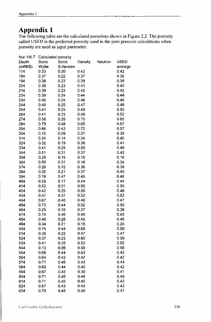
Appendix 1
Appendix 1 The following table are the calculated porosities shown in Figure 2.2. The porosity called USED is the preferred porosity used in the pore pressure calculations when porosity are used as input parameter.
Nor-1/6-7 Calculated porosity Depth Sonic Sonic Density Neutron USED (mRKB) Wyllie S.Hansen average 174 0.33 0.20 0.42 0.42 184 0.37 0.22 0.37 0.36 194 0.38 0.23 0.39 0.38 204 0.38 0.23 0.41 0.40 214 0.39 0.23 0.42 0.42 224 0.39 0.24 0.44 0.44 234 0.40 0.24 0.46 0.46 244 0.40 0.25 0.47 0.48 254 0.41 0.25 0.49 0.50 264 0.41 0.25 0.50 0.52 274 0.58 0.35 0.75 0.65 284 0.79 0.48 0.65 0.57 294 0.66 0.43 0.72 0.57 304 0.15 0.09 0.31 0.39 314 0.24 0.14 0.34 0.40 324 0.32 0.19 0.38 0.41 334 0.41 0.25 0.50 0.49 344 0.51 0.31 0.37 0.43 354 0.25 0.15 0.15 0.16 364 0.50 0.31 0.18 0.34 374 0.20 0.12 0.36 0.39 384 0.35 0.21 0.37 0.40 394 0.78 0.47 0.45 0.46 404 0.28 0.17 0.44 0.44 414 0.52 0.31 0.50 0.50 424 0.42 0.25 0.50 0.48 434 0.51 0.31 0.52 0.52 444 0.67 0.40 0.46 0.47 454 0.73 0.44 0.52 0.50 464 0.25 0.15 0.37 0.38 474 0.74 0.46 0.40 0.43 484 0.46 0.28 0.45 0.46 494 0.34 0.21 0.18 0.24 504 0.75 0.44 0.69 0.60 514 0.36 0.22 0.47 0.47 524 0.37 0.22 0.60 0.59 534 0.41 0.25 0.52 0.52 544 0.13 0.08 0.58 0.58 554 0.68 0.44 0.43 0.43 564 0.64 0.42 0.42 0.42 574 0.71 0.45 0.43 0.44 584 0.69 0.44 0.40 0.42 594 0.67 0.43 0.39 0.41 604 0.71 0.45 0.44 0.45 614 0.71 0.45 0.40 0.43 624 0.67 0.43 0.43 0.43 634 0.70 0.45 0.49 0.47
Car l Freclrik G y l l e n h a m m a i " 136

Appendix 1
644 0.69 0.44 654 0.70 0.45 664 0.67 0.44 674 0.68 0.44 684 0.71 0.45 694 0.70 0.45 704 0.70 0.45 714 0.79 0.48 724 0.67 0.43 734 0.68 0.44 744 0.74 0.46 754 0.68 0.44 764 0.68 0.44 774 0.71 0.45 784 0.65 0.42 794 0.61 0.41 804 0.64 0.42 814 0.64 0.42 824 0.66 0.43 834 0.67 0.43 844 0.69 0.44 854 0.69 0.44 864 0.73 0.46 874 0.67 0.43 884 0.71 0.45 894 0.67 0.43 904 0.64 0.42 914 0.68 0.44 924 0.67 0.43 934 0.68 0.44 944 0.62 0.41 954 0.64 0.42 964 0.66 0.43 974 0.61 0.41 984 0.63 0.42 994 0.62 0.41 1004 0.64 0.42 1014 0.66 0.43 1024 0.67 0.43 1034 0.62 0.41 1044 0.66 0.43 1054 0.62 0.41 1064 0.66 0.43 1074 0.66 0.43 1084 0.60 0.41 1094 0.69 0.44 1104 0.66 0.43 1114 0.67 0.43 1124 0.66 0.43 1134 0.65 0.42 1144 0.68 0.44 1154 0.66 0.43 1164 0.67 0.43 1174 0.67 0.43 1184 0.64 0.42 1194 0.61 0.41
0.42 0.43 0.43 0.44 0.44 0.44 0.43 0.43 0.42 0.44 0.40 0.42 0.41 0.43 0.43 0.45 0.40 0.42 0.44 0.44 0.46 0.46 0.40 0.42 0.41 0.42 0.43 0.44 0.41 0.42 0.41 0.41 0.43 0.42 0.40 0.41 0.40 0.42 0.43 0.43 0.42 0.43 0.48 0.46 0.43 0.45 0.41 0.42 0.48 0.46 0.41 0.42 0.41 0.42 0.41 0.42 0.40 1.12 0.41 0.43 1.00 0.44 0.38 1.05 0.40 0.38 0.97 0.40 0.40 1.01 0.42 0.38 0.93 0.39 0.38 0.89 0.40 0.00 0.98 0.41 0.43 0.80 0.43 0.42 0.69 0.43 0.40 0.81 0.42 0.40 0.78 0.41 0.39 0.74 0.41 0.41 0.70 0.41 0.40 0.64 0.42 0.41 0.69 0.42 0.42 0.71 0.41 0.46 0.90 0.45 0.45 0.68 0.44 0.44 0.70 0.44 0.43 0.77 0.43 0.44 0.82 0.43 0.44 0.77 0.44 0.44 0.74 0.44 0.43 0.75 0.43 0.46 0.78 0.44 0.42 0.81 0.42 0.40 0.74 0.41
Car l F r e d r i k G y l l e n h a m m a r 137
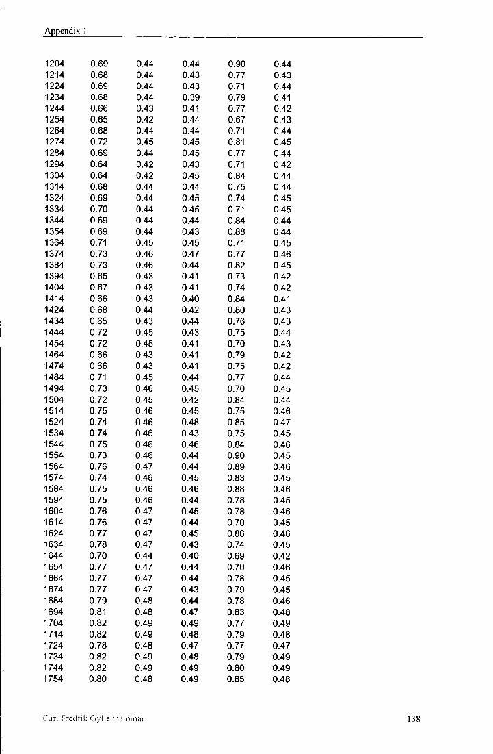
Appendix 1
1204 0.69 0.44 1214 0.68 0.44 1224 0.69 0.44 1234 0.68 0.44 1244 0.66 0.43 1254 0.65 0.42 1264 0.68 0.44 1274 0.72 0.45 1284 0.69 0.44 1294 0.64 0.42 1304 0.64 0.42 1314 0.68 0.44 1324 0.69 0.44 1334 0.70 0.44 1344 0.69 0.44 1354 0.69 0.44 1364 0.71 0.45 1374 0.73 0.46 1384 0.73 0.46 1394 0.65 0.43 1404 0.67 0.43 1414 0.66 0.43 1424 0.68 0.44 1434 0.65 0.43 1444 0.72 0.45 1454 0.72 0.45 1464 0.66 0.43 1474 0.66 0.43 1484 0.71 0.45 1494 0.73 0.46 1504 0.72 0.45 1514 0.75 0.46 1524 0.74 0.46 1534 0.74 0.46 1544 0.75 0.46 1554 0.73 0.46 1564 0.76 0.47 1574 0.74 0.46 1584 0.75 0.46 1594 0.75 0.46 1604 0.76 0.47 1614 0.76 0.47 1624 0.77 0.47 1634 0.78 0.47 1644 0.70 0.44 1654 0.77 0.47 1664 0.77 0.47 1674 0.77 0.47 1684 0.79 0.48 1694 0.81 0.48 1704 0.82 0.49 1714 0.82 0.49 1724 0.78 0.48 1734 0.82 0.49 1744 0.82 0.49 1754 0.80 0.48
0.44 0.90 0.44 0.43 0.77 0.43 0.43 0.71 0.44 0.39 0.79 0.41 0.41 0.77 0.42 0.44 0.67 0.43 0.44 0.71 0.44 0.45 0.81 0.45 0.45 0.77 0.44 0.43 0.71 0.42 0.45 0.84 0.44 0.44 0.75 0.44 0.45 0.74 0.45 0.45 0.71 0.45 0.44 0.84 0.44 0.43 0.88 0.44 0.45 0.71 0.45 0.47 0.77 0.46 0.44 0.82 0.45 0.41 0.73 0.42 0.41 0.74 0.42 0.40 0.84 0.41 0.42 0.80 0.43 0.44 0.76 0.43 0.43 0.75 0.44 0.41 0.70 0.43 0.41 0.79 0.42 0.41 0.75 0.42 0.44 0.77 0.44 0.45 0.70 0.45 0.42 0.84 0.44 0.45 0.75 0.46 0.48 0.85 0.47 0.43 0.75 0.45 0.46 0.84 0.46 0.44 0.90 0.45 0.44 0.89 0.46 0.45 0.83 0.45 0.46 0.88 0.46 0.44 0.78 0.45 0.45 0.78 0.46 0.44 0.70 0.45 0.45 0.86 0.46 0.43 0.74 0.45 0.40 0.69 0.42 0.44 0.70 0.46 0.44 0.78 0.45 0.43 0.79 0.45 0.44 0.78 0.46 0.47 0.83 0.48 0.49 0.77 0.49 0.48 0.79 0.48 0.47 0.77 0.47 0.48 0.79 0.49 0.49 0.80 0.49 0.49 0.85 0.48
C a r l Fredr ik G y l l e n h a m m a r 138
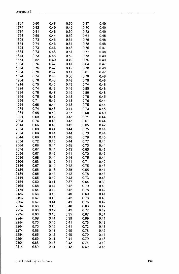
Appendix 1
1764 0.80 0.48 0.50 0.87 0.49 1774 0.82 0.49 0.49 0.80 0.49 1784 0.81 0.48 0.50 0.83 0.49 1794 0.69 0.44 0.52 0.61 0.48 1804 0.73 0.46 0.51 0.75 0.48 1814 0.74 0.46 0.51 0.78 0.48 1824 0.73 0.46 0.48 0.75 0.47 1834 0.73 0.46 0.51 0.77 0.48 1844 0.73 0.46 0.52 0.73 0.49 1854 0.82 0.49 0.49 0.75 0.49 1864 0.76 0.47 0.47 0.84 0.47 1874 0.76 0.47 0.49 0.76 0.48 1884 0.76 0.47 0.47 0.81 0.47 1894 0.74 0.46 0.50 0.79 0.48 1904 0.78 0.48 0.48 0.79 0.48 1914 0.75 0.46 0.49 0.74 0.48 1924 0.74 0.46 0.49 0.85 0.48 1934 0.78 0.47 0.49 0.80 0.48 1944 0.76 0.47 0.43 0.78 0.45 1954 0.71 0.45 0.43 0.76 0.44 1964 0.68 0.44 0.43 0.75 0.44 1974 0.74 0.46 0.44 0.73 0.45 1984 0.65 0.42 0.37 0.68 0.40 1994 0.69 0.44 0.43 0.71 0.44 2004 0.74 0.46 0.43 0.67 0.44 2014 0.66 0.43 0.42 0.65 0.42 2024 0.69 0.44 0.44 0.75 0.44 2034 0.68 0.44 0.44 0.73 0.44 2044 0.68 0.44 0.46 0.79 0.45 2054 0.72 0.45 0.44 0.77 0.44 2064 0.68 0.44 0.45 0.73 0.44 2074 0.67 0.44 0.43 0.65 0.43 2084 0.67 0.43 0.41 0.70 0.42 2094 0.68 0.44 0.44 0.75 0.44 2104 0.63 0.42 0.41 0.71 0.42 2114 0.67 0.44 0.42 0.75 0.43 2124 0.66 0.43 0.38 0.65 0.41 2134 0.68 0.44 0.42 0.78 0.43 2144 0.65 0.42 0.43 0.73 0.43 2154 0.60 0.41 0.37 0.64 0.39 2164 0.68 0.44 0.42 0.79 0.43 2174 0.64 0.42 0.42 0.78 0.42 2184 0.66 0.43 0.40 0.69 0.41 2194 0.67 0.43 0.42 0.78 0.43 2204 0.67 0.44 0.41 0.78 0.42 2214 0.66 0.43 0.40 0.66 0.42 2224 0.63 0.42 0.42 0.72 0.42 2234 0.60 0.40 0.35 0.67 0.37 2244 0.69 0.44 0.39 0.69 0.41 2254 0.70 0.45 0.41 0.75 0.43 2264 0.70 0.45 0.41 0.72 0.43 2274 0.68 0.44 0.40 0.78 0.42 2284 0.65 0.42 0.40 0.70 0.41 2294 0.69 0.44 0.41 0.70 0.43 2304 0.66 0.43 0.42 0.76 0.42 2314 0.69 0.44 0.42 0.69 0.43
C a r l F redr ik G y l l e n h a m m a r 139

Appendix 1
2324 0.68 0.44 0.42 0.76 0.43 2334 0.68 0.44 0.42 0.72 0.43 2344 0.69 0.44 0.42 0.74 0.43 2354 0.60 0.40 0.40 0.64 0.40 2364 0.67 0.43 0.44 0.76 0.44 2374 0.66 0.43 0.41 0.71 0.42 2384 0.68 0.44 0.42 0.80 0.43 2394 0.64 0.42 0.41 0.71 0.41 2404 0.71 0.45 0.43 0.71 0.44 2414 0.70 0.45 0.42 0.71 0.43 2424 0.68 0.44 0.40 0.71 0.42 2434 0.73 0.45 0.44 0.77 0.45 2444 0.64 0.42 0.36 0.70 0.39 2454 0.64 0.42 0.39 0.67 0.40 2464 0.61 0.41 0.32 0.66 0.36 2474 0.71 0.45 0.35 0.65 0.40 2484 0.68 0.44 0.40 0.74 0.42 2494 0.71 0.45 0.39 0.65 0.42 2504 0.67 0.43 0.38 0.67 0.40 2514 0.67 0.43 0.39 0.66 0.41 2524 0.65 0.43 0.34 0.71 0.39 2534 0.63 0.42 0.37 0.70 0.39 2544 0.64 0.42 0.35 0.61 0.38 2554 0.62 0.41 0.34 0.61 0.37 2564 0.69 0.44 0.39 0.68 0.42 2574 0.66 0.43 0.37 0.67 0.40 2584 0.68 0.44 0.38 0.74 0.41 2594 0.65 0.43 0.37 0.66 0.40 2604 0.61 0.41 0.36 0.66 0.38 2614 0.59 0.40 0.35 0.58 0.37 2624 0.63 0.42 0.34 0.66 0.38 2634 0.63 0.42 0.38 0.70 0.40 2644 0.63 0.42 0.36 0.72 0.39 2654 0.60 0.40 0.35 0.66 0.38 2664 0.58 0.40 0.32 0.72 0.36 2674 0.59 0.40 0.33 0.63 0.37 2684 0.58 0.39 0.36 0.62 0.38 2694 0.54 0.38 0.29 0.62 0.33 2704 0.53 0.37 0.32 0.61 0.34 2714 0.54 0.38 0.32 0.63 0.35 2724 0.56 0.39 0.34 0.70 0.36 2734 0.54 0.38 0.29 0.62 0.33 2744 0.57 0.39 0.32 0.60 0.36 2754 0.54 0.38 0.30 0.62 0.34 2764 0.51 0.36 0.29 0.55 0.32 2774 0.53 0.37 0.29 0.56 0.33 2784 0.48 0.34 0.35 0.69 0.35 2794 0.56 0.38 0.36 0.62 0.37 2804 0.45 0.33 0.33 0.73 0.33 2814 0.53 0.37 0.34 0.70 0.35 2824 0.56 0.38 0.32 0.66 0.35 2834 0.53 0.37 0.30 0.69 0.33 2844 0.59 0.40 0.33 0.75 0.36 2854 0.51 0.36 0.29 0.55 0.32 2864 0.54 0.38 0.32 0.62 0.35 2874 0.52 0.37 0.30 0.56 0.33
C a r l F r e d r i k G y l l e n h a m m a r 140
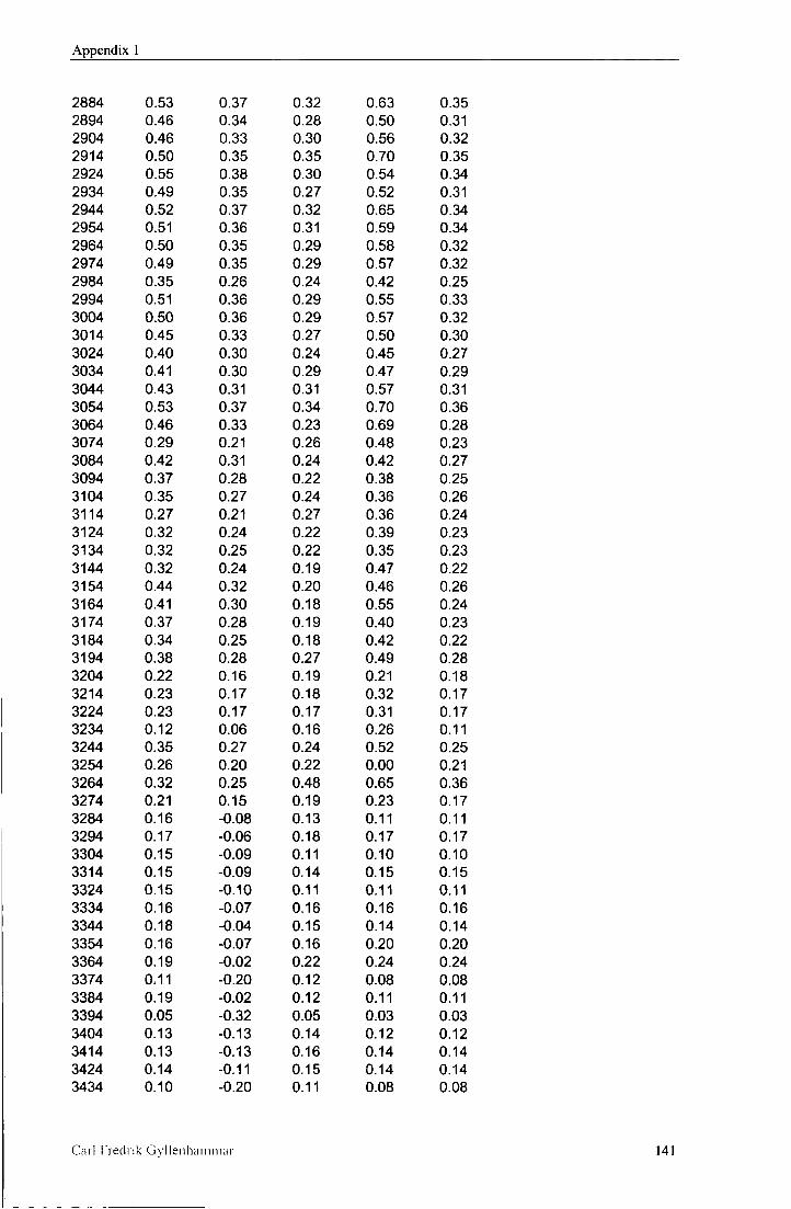
Appendix 1
2884 2894 2904 2914 2924 2934 2944 2954 2964 2974 2984 2994 3004 3014 3024 3034 3044 3054 3064 3074 3084 3094 3104 3114 3124 3134 3144 3154 3164 3174 3184 3194 3204 3214 3224 3234 3244 3254 3264 3274 3284 3294 3304 3314 3324 3334 3344 3354 3364 3374 3384 3394 3404 3414 3424 3434
0.53 0.46 0.46 0.50 0.55 0.49 0.52 0.51 0.50 0.49 0.35 0.51 0.50 0.45 0.40 0.41 0.43 0.53 0.46 0.29 0.42 0.37 0.35 0.27 0.32 0.32 0.32 0.44 0.41 0.37 0.34 0.38 0.22 0.23 0.23 0.12 0.35 0.26 0.32 0.21 0.16 0.17 0.15 0.15 0.15 0.16 0.18 0.16 0.19 0.11 0.19 0.05 0.13 0.13 0.14 0.10
0.37 0.34 0.33 0.35 0.38 0.35 0.37 0.36 0.35 0.35 0.26 0.36 0.36 0.33 0.30 0.30 0.31 0.37 0.33 0.21 0.31 0.28 0.27 0.21 0.24 0.25 0.24 0.32 0.30 0.28 0.25 0.28 0.16 0.17 0.17 0.06 0.27 0.20 0.25 0.15 -0.08 -0.06 -0.09 -0.09 -0.10 -0.07 -0.04 -0.07 -0.02 -0.20 -0.02 -0.32 -0.13 -0.13 -0.11 -0.20
0.32 0.28 0.30 0.35 0.30 0.27 0.32 0.31 0.29 0.29 0.24 0.29 0.29 0.27 0.24 0.29 0.31 0.34 0.23 0.26 0.24 0.22 0.24 0.27 0.22 0.22 0.19 0.20 0.18 0.19 0.18 0.27 0.19 0.18 0.17 0.16 0.24 0.22 0.48 0.19 0.13 0.18 0.11 0.14 0.11 0.16 0.15 0.16 0.22 0.12 0.12 0.05 0.14 0.16 0.15 0.11
0.63 0.50 0.56 0.70 0.54 0.52 0.65 0.59 0.58 0.57 0.42 0.55 0.57 0.50 0.45 0.47 0.57 0.70 0.69 0.48 0.42 0.38 0.36 0.36 0.39 0.35 0.47 0.46 0.55 0.40 0.42 0.49 0.21 0.32 0.31 0.26 0.52 0.00 0.65 0.23 0.11 0.17 0.10 0.15 0.11 0.16 0.14 0.20 0.24 0.08 0.11 0.03 0.12 0.14 0.14 0.08
0.35 0.31 0.32 0.35 0.34 0.31 0.34 0.34 0.32 0.32 0.25 0.33 0.32 0.30 0.27 0.29 0.31 0.36 0.28 0.23 0.27 0.25 0.26 0.24 0.23 0.23 0.22 0.26 0.24 0.23 0.22 0.28 0.18 0.17 0.17 0.11 0.25 0.21 0.36 0.17 0.11 0.17 0.10 0.15 0.11 0.16 0.14 0.20 0.24 0.08 0.11 0.03 0.12 0.14 0.14 0.08
Car l Fredr ik G y l l e n h a m m a r 141
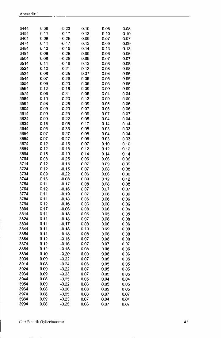
Appendix 1
3444 0.09 3454 0.11 3464 0.08 3474 0.11 3484 0.12 3494 0.08 3504 0.08 3514 0.11 3524 0.10 3534 0.08 3544 0.07 3554 0.09 3564 0.12 3574 0.06 3584 0.10 3594 0.08 3604 0.09 3614 0.09 3624 0.09 3634 0.16 3644 0.05 3654 0.07 3664 0.07 3674 0.12 3684 0.12 3694 0.15 3704 0.08 3714 0.12 3724 0.12 3734 0.09 3744 0.16 3754 0.11 3764 0.12 3774 0.11 3784 0.11 3794 0.12 3804 0.17 3814 0.11 3824 0.11 3834 0.11 3844 0.11 3854 0.11 3864 0.12 3874 0.12 3884 0.12 3894 0.10 3904 0.09 3914 0.08 3924 0.09 3934 0.09 3944 0.08 3954 0.09 3964 0.08 3974 0.08 3984 0.09 3994 0.08
-0.23 0.10 -0.17 0.13 -0.25 0.09 -0.17 0.12 -0.15 0.14 -0.25 0.09 -0.25 0.09 -0.19 0.12 -0.21 0.12 -0.25 0.07 -0.29 0.06 -0.23 0.06 -0.16 0.09 -0.31 0.06 -0.20 0.13 -0.25 0.09 -0.23 0.07 -0.23 0.09 -0.22 0.05 -0.08 0.17 -0.35 0.05 -0.27 0.08 -0.27 0.05 -0.15 0.07 -0.16 0.12 -0.10 0.14 -0.25 0.06 -0.15 0.07 -0.15 0.07 -0.22 0.06 -0.08 0.09 -0.17 0.08 -0.16 0.07 -0.19 0.07 -0.18 0.06 -0.16 0.06 -0.06 0.08 -0.18 0.06 -0.18 0.07 -0.17 0.08 -0.18 0.10 -0.18 0.08 -0.15 0.07 -0.16 0.07 -0.15 0.08 -0.20 0.09 -0.22 0.07 -0.24 0.06 -0.22 0.07 -0.23 0.07 -0.25 0.05 -0.22 0.06 -0.26 0.08 -0.25 0.08 -0.23 0.07 -0.25 0.08
0.08 0.08 0.10 0.10 0.07 0.07 0.09 0.09 0.13 0.13 0.06 0.06 0.07 0.07 0.08 0.08 0.08 0.08 0.06 0.06 0.05 0.05 0.05 0.05 0.09 0.09 0.04 0.04 0.09 0.09 0.06 0.06 0.06 0.06 0.07 0.07 0.04 0.04 0.14 0.14 0.03 0.03 0.04 0.04 0.03 0.03 0.10 0.10 0.12 0.12 0.14 0.14 0.06 0.06 0.09 0.09 0.08 0.08 0.06 0.06 0.12 0.12 0.08 0.08 0.07 0.07 0.06 0.06 0.06 0.06 0.06 0.06 0.06 0.06 0.05 0.05 0.08 0.08 0.06 0.06 0.09 0.09 0.08 0.08 0.08 0.08 0.07 0.07 0.06 0.06 0.06 0.06 0.05 0.05 0.05 0.05 0.05 0.05 0.05 0.05 0.04 0.04 0.05 0.05 0.05 0.05 0.07 0.07 0.04 0.04 0.07 0.07
Car l F red r ik G y l l e n h a m m a r 142

Appendix 1
4004 0.08 -0.25 4014 0.06 -0.30 4024 0.10 -0.21 4034 0.11 -0.17 4044 0.12 -0.16 4054 0.11 -0.18 4064 0.09 -0.23 4074 0.08 -0.26 4084 0.07 -0.27 4094 0.08 -0.24 4104 0.12 -0.17 4114 0.08 -0.24 4124 0.09 -0.24 4134 0.10 -0.21 4144 0.15 -0.11 4154 0.06 -0.02 4164 0.09 -0.23 4174 0.11 -0.17 4184 0.11 -0.17 4194 0.16 -0.07 4204 0.11 -0.19 4214 0.13 -0.14 4224 0.15 -0.10 4234 0.12 -0.16 4244 0.12 -0.16 4254 0.12 -0.15 4264 0.13 -0.15 4274 0.11 -0.17 4284 0.14 -0.12 4294 0.03 -0.07 4304 0.10 0.03 4314 0.15 0.08 4324 0.15 0.08 4334 0.15 0.08 4344 0.23 0.16 4354 0.34 0.26 4364 0.43 0.31 4374 0.29 0.22 4384 0.28 0.21 4394 0.27 0.20 4404 0.45 0.33 4414 0.48 0.35 4424 0.52 0.37 4434 0.45 0.33 4444 0.36 0.26 4454 0.40 0.30 4464 0.49 0.35 4474 0.58 0.39 4484 0.64 0.42 4494 0.56 0.39 4504 0.53 0.37 4514 0.51 0.36 4524 0.64 0.42 4534 0.50 0.35 4544 0.48 0.34 4554 0.51 0.36
0.05 0.03 0.03 0.07 0.04 0.04 0.07 0.04 0.04 0.07 0.05 0.05 0.02 0.03 0.03 0.10 0.10 0.10 0.04 0.03 0.03 0.07 0.07 0.07 0.06 0.06 0.06 0.07 0.07 0.07 0.08 0.09 0.09 0.08 0.08 0.08 0.09 0.09 0.09 0.06 0.07 0.07 0.07 0.10 0.10 0.11 0.12 0.11 0.09 0.07 0.07 0.08 0.10 0.10 0.06 0.07 0.07 0.06 0.12 0.12 0.06 0.07 0.07 0.06 0.09 0.09 0.05 0.10 0.10 0.08 0.11 0.11 0.09 0.12 0.12 0.07 0.08 0.08 0.09 0.09 0.09 0.08 0.08 0.08 0.08 0.09 0.09 0.11 0.11 0.11 0.11 0.14 0.11 0.15 0.26 0.15 0.26 0.44 0.26 0.25 0.24 0.25 0.10 0.09 0.10 0.20 0.45 0.20 0.26 0.41 0.26 0.26 0.28 0.26 0.24 0.24 0.24 0.21 0.24 0.21 0.23 0.35 0.23 0.23 0.35 0.23 0.22 0.33 0.22 0.25 0.32 0.25 0.19 0.26 0.19 0.20 0.26 0.20 0.27 0.32 0.27 0.32 0.35 0.32 0.30 0.33 0.30 0.28 0.33 0.28 0.32 0.33 0.32 0.33 0.35 0.33 0.30 0.34 0.30 0.27 0.33 0.27 0.28 0.32 0.28 0.32 0.37 0.32
Car l I - red] ik G y l l e n h a m m a r 143

4564 0.49 4574 0.15 4584 0.54 4594 0.51 4604 0.52 4614 0.54 4624 0.57 4634 0.59 4644 0.54 4654 0.53 4664 0.46 4674 0.42 4684 0.42 4694 0.39 4704 0.34 4714 0.31 4724 0.32 4734 0.34 4744 0.29 4754 0.35 4764 0.32 4774 0.35 4784 0.35 4794 0.28 4804 0.25 4814 0.29 4824 0.30 4834 0.24 4844 0.25 4854 0.24 4864 0.28 4874 0.42 4884 0.27 4894 0.29 4904 0.32 4914 0.28 4924 0.26 4934 0.26 4944 0.23 4954 0.24 4964 0.24 4974 0.23 4984 0.19 4994 0.17
0.35 0.24 0.04 0.06 0.37 0.27 0.36 0.28 0.37 0.29 0.37 0.25 0.39 0.28 0.40 0.28 0.38 0.27 0.37 0.27 0.34 0.25 0.31 0.26 0.31 0.25 0.29 0.24 0.26 0.24 0.24 0.24 0.24 0.22 0.26 0.24 0.22 0.22 0.21 0.18 0.19 0.17 0.21 0.16 0.21 0.15 0.21 0.23 0.18 0.21 0.21 0.21 0.22 0.20 0.17 0.20 0.18 0.21 0.17 0.21 0.20 0.20 0.30 0.20 0.13 0.25 0.16 0.24 0.18 0.24 0.14 0.18 0.12 0.23 0.12 0.22 0.09 0.20 0.10 0.21 0.10 0.24 0.09 0.22 0.12 0.15 0.11 0.18
0.30 0.24 0.12 0.06 0.34 0.27 0.33 0.28 0.34 0.29 0.33 0.25 0.33 0.28 0.34 0.28 0.36 0.27 0.36 0.27 0.31 0.25 0.26 0.26 0.27 0.25 0.25 0.24 0.23 0.24 0.22 0.24 0.24 0.22 0.24 0.24 0.22 0.22 0.23 0.20 0.23 0.20 0.25 0.21 0.24 0.20 0.21 0.23 0.19 0.21 0.21 0.21 0.24 0.20 0.20 0.20 0.21 0.21 0.20 0.21 0.22 0.20 0.28 0.20 0.19 0.22 0.19 0.22 0.20 0.22 0.18 0.18 0.17 0.20 0.17 0.20 0.18 0.19 0.17 0.19 0.16 0.20 0.17 0.20 0.23 0.15 0.23 0.18
G i r l F redr ik G y l l e n h a m m a r 144

Appendix 2
Appendix 2 The following table are the wireline data with the calculated pore pressure values used in Figure 3.9, 3.10, 3.11, 3.12, 3.13, 3.14 and 3.15.
Well Nor-1/6-7 Overbur Hydrost PORE PRESSURE CALCULATION den atic
Water D 69.80 (m) Porosity pressure pressure Toby Equivalent depth Eaton method metod
RKB 22.00 (m) USED Univers Burland Athy Sonic Resistiv ity ity
Depth HDEN HRD HAC HGR Durham Compaction trend (mRKB) g/cc ohmm usec/ft api MPa MPa MPa MPa MPa MPa MPa
92 4 0.8 0.8 0.0 0.7 93 5 0.8 0.8 0.0 0.7 94 5 0.8 0.8 0.0 0.7 95 5 0.9 0.8 0.0 0.8 96 5 0.9 0.9 0.0 0.8 97 5 0.9 0.9 0.0 0.8 98 6 0.9 0.9 0.0 0.8 99 5 0.9 0.9 0.0 0.8
110 5 1.1 1.0 0.0 0.0 0.0 0.0 1.0 120 6 1.3 1.1 0.0 0.0 0.0 0.0 1.2 130 7 1.5 1.2 0.0 0.0 0.0 0.0 1.4 140 6 1.7 1.3 0.0 0.0 0.0 0.0 1.6 150 12 1.8 1.4 0.0 0.0 0.0 0.0 1.7 160 13 0.13 2.0 1.5 0.0 0.0 0.0 0.0 1.9 170 1.96 0.0 46 0.48 2.2 1.6 -2.6 -1.2 -8.7 0.0 2.1 180 1.54 167.0 58 0.36 2.4 1.7 -14.9 -9.4 -1.5 1.5 2.3 190 8 0.00 2.6 1.8 0.0 0.0 0.0 0.0 2.5 200 9 0.00 2.8 1.9 0.0 0.0 0.0 0.0 2.7 210 8 0.00 2.9 2.0 0.0 0.0 0.0 0.0 2.8 220 9 0.00 3.1 2.1 0.0 0.0 0.0 0.0 3.0 230 9 0.00 3.3 2.2 0.0 0.0 0.0 0.0 3.2 240 9 0.00 3.5 2.3 0.0 0.0 0.0 0.0 3.4 250 10 0.00 3.6 2.5 0.0 0.0 0.0 0.0 3.5 260 11 0.00 3.8 2.6 0.0 0.0 0.0 0.0 3.7 270 67 0.37 4.0 2.7 -11.7 -6.9 -2.0 2.3 3.9 280 1.83 75 0.56 4.2 2.8 3.0 2.9 -3.0 2.5 4.1 290 1.62 167.0 62 0.56 4.4 2.9 3.4 3.2 4.3 2.6 4.3 300 1.71 71 0.58 4.5 3.0 4.0 3.7 13.0 2.7 4.4 310 1.61 68 0.27 4.7 3.1 -26.7 -16.8 9.4 2.8 4.6 320 9 0.00 4.9 3.2 0.0 0.0 0.0 0.0 4.8 330 2.07 160.0 76 0.45 5.1 3.3 -1.7 0.0 -3.1 2.8 5.0 340 14 0.04 5.3 3.4 0.0 0.0 0.0 0.6 5.2 350 2.04 88 0.40 5.4 3.5 -5.5 -2.5 -4.7 3.2 5.4 360 11 0.00 5.6 3.6 0.0 0.0 0.0 0.0 5.5 370 66 0.39 5.8 3.7 -6.3 -2.9 -3.9 3.2 5.7 380 7 0.00 6.0 3.8 0.0 0.0 0.0 0.0 5.9 390 2.17 79 0.41 6.2 3.9 -4.2 -1.5 -1.1 3.6 6.1 400 1.98 73 0.44 6.4 4.0 -1.2 0.6 -1.2 3.7 6.3 410 1.80 77 0.55 6.5 4.1 5.7 5.2 1.2 3.8 6.4 420 2.02 159.4 77 0.46 6.7 4.2 1.2 2.2 0.2 3.6 6.6 430 1.82 166.4 82 0.48 6.9 4.3 2.7 3.3 -0.4 4.0 6.8 440 2.06 164.1 87 0.43 7.1 4.4 -0.5 1.1 -1.0 4.0 7.0 450 1.96 58 0.53 7.3 4.5 5.8 5.4 7.0 4.2 7.2
C a r l F r e d r i k G y H e n h a m m a r 145

Appendix 2
460 2.06 154.6 75 0.45 7.5 4.6 1.7 2.7 0.1 3.8 7.4 470 1.56 48 0.64 7.7 4.7 8.6 7.3 4.8 0.0 7.6 480 1.82 58 0.43 7.9 4.8 0.3 1.8 1.9 4.6 7.8 490 2.00 44 0.53 8.1 4.9 6.6 6.1 18.5 0.0 8.0 500 1.57 20 0.70 8.2 5.0 0.0 0.0 0.0 0.0 8.2 510 1.59 20 0.70 8.4 5.2 0.0 0.0 0.0 0.0 8.3 520 2.06 156.2 89 0.45 8.6 5.3 2.8 3.6 -0.1 4.5 8.5 530 1.87 33 0.56 8.8 5.4 8.5 7.4 11.5 1.0 8.7 540 1.63 31 0.64 9.0 5.5 10.1 8.6 4.8 0.9 8.9 550 2.06 156.9 63 0.44 9.2 5.6 2.1 3.3 -0.4 4.6 9.1 560 2.08 150.3 67 0.43 9.4 5.7 1.7 3.0 -1.2 4.5 9.3 570 2.06 151.1 64 0.44 9.6 5.8 2.7 3.7 0.7 4.4 9.5 580 1.89 152.6 71 0.49 9.8 5.9 6.7 6.4 -0.2 4.7 9.7 590 2.01 153.8 68 0.44 10.0 6.0 3.2 4.1 0.3 4.6 9.9 600 2.11 150.4 72 0.41 10.2 6.1 1.1 2.8 -0.3 4.5 10.1 610 2.04 149.3 71 0.43 10.4 6.2 3.6 4.4 -1.3 4.9 10.3 620 2.07 132.1 76 0.40 10.6 6.3 0.7 2.6 1.9 3.0 10.5 630 1.87 156.6 58 0.48 10.8 6.4 7.4 7.1 4.6 5.6 10.7 640 2.01 146.0 63 0.43 11.0 6.5 4.3 5.0 3.8 4.8 10.9 650 2.01 157.7 77 0.45 11.2 6.6 5.9 6.1 2.6 5.9 11.1 660 2.07 146.7 69 0.42 11.4 6.7 3.7 4.7 1.0 5.0 11.3 670 2.01 154.4 71 0.46 11.6 6.8 7.4 7.2 3.9 5.8 11.5 680 1.97 158.6 81 0.46 11.8 6.9 7.1 7.1 1.9 6.3 11.7 690 2.04 156.9 89 0.44 12.0 7.0 6.1 6.4 2.5 6.2 11.9 700 2.10 152.9 77 0.42 12.2 7.1 4.7 5.5 2.0 5.9 12.1 710 2.04 151.9 73 0.44 12.4 7.2 6.4 6.7 4.1 4.7 12.3 720 2.07 155.0 86 0.44 12.6 7.3 6.8 7.0 3.7 6.5 12.5 730 2.12 146.7 67 0.41 12.8 7.4 3.8 5.0 1.2 5.6 12.7 740 2.09 145.6 79 0.43 13.0 7.5 6.4 6.8 3.3 5.5 12.9 750 2.09 155.1 78 0.43 13.2 7.6 6.3 6.7 4.2 6.7 13.1 760 2.13 146.1 68 0.41 13.4 7.8 4.7 5.7 -0.5 5.5 13.3 770 1.99 152.9 79 0.45 13.6 7.9 8.8 8.5 4.0 6.7 13.5 780 2.07 149.0 66 0.43 13.8 8.0 7.0 7.3 3.9 6.3 13.7 790 2.08 150.6 74 0.43 14.0 8.1 7.5 7.7 3.5 6.7 13.9 800 2.04 149.5 72 0.44 14.2 8.2 8.6 8.5 5.2 6.5 14.1 810 2.08 148.9 69 0.42 14.4 8.3 7.5 7.8 4.1 6.6 14.3 820 2.08 145.9 71 0.42 14.6 8.4 6.8 7.3 4.1 6.2 14.5 830 2.08 150.9 76 0.43 14.8 8.5 8.3 8.4 3.9 7.0 14.7 840 2.11 150.0 86 0.42 15.0 8.6 7.5 7.8 4.2 7.0 14.9 850 2.11 149.1 74 0.41 15.2 8.7 7.4 7.8 4.7 7.0 15.1 860 2.02 152.7 97 0.45 15.4 8.8 10.7 10.0 6.6 7.7 15.3 870 2.12 146.3 76 0.41 15.6 8.9 7.1 7.7 3.5 7.0 15.5 880 2.05 150.6 76 0.43 15.8 9.0 9.8 9.6 5.2 7.6 15.7 890 2.10 136.9 80 0.41 16.0 9.1 8.2 8.5 5.0 6.0 15.9 900 2.09 146.6 77 0.42 16.2 9.2 9.0 9.0 5.3 7.2 16.1 910 2.10 147.2 83 0.41 16.4 9.3 8.8 8.9 4.5 7.3 16.3 920 2.11 148.1 76 0.41 16.6 9.4 8.9 9.1 5.2 7.7 16.5 930 2.09 147.3 74 0.41 16.8 9.5 9.5 9.5 5.1 7.6 940 2.07 155.0 97 0.43 17.0 9.6 11.4 10.8 7.1 8.9 950 2.13 146.9 82 0.40 17.2 9.7 8.9 9.2 4.9 8.0 960 2.11 143.9 71 0.41 17.4 9.8 10.0 9.9 4.2 7.4 970 2.10 145.9 82 0.42 17.6 9.9 10.6 10.4 6.1 8.2 980 2.13 145.6 70 0.40 17.9 10.0 9.7 9.8 5.1 8.0 990 2.10 145.1 51 0.41 18.1 10.1 10.4 10.3 5.7 6.3
1000 144.2 46 0.37 18.3 10.2 5.8 7.3 7.1 0.0 1010 2.12 0.78 145.5 70 0.42 18.5 10.3 11.6 11.2 8.9 8.3 16.0
Car l F red r ik G y l l e n h a m m a r 146

Appendix 2
1020 2.12 0.77 149.9 82 0.42 18.7 10.5 12.1 11.5 7.1 9.4 16.2 1030 2.06 0.80 150.0 86 0.43 18.9 10.6 13.1 12.3 8.3 9.3 16.2 1040 2.08 1.02 146.7 77 0.42 19.1 10.7 12.6 12.0 7.8 8.9 15.6 1050 2.04 0.83 149.5 82 0.44 19.3 10.8 14.5 13.3 9.0 9.5 16.6 1060 2.11 0.92 141.3 71 0.40 19.5 10.9 11.3 11.2 7.2 8.3 16.3 1070 2.01 0.81 149.4 81 0.44 19.7 11.0 15.1 13.7 10.1 9.8 16.9 1080 2.11 0.75 140.7 72 0.41 19.9 11.1 12.3 11.9 6.8 8.2 17.3 1090 2.05 0.72 149.2 84 0.43 20.1 11.2 15.1 13.8 9.4 10.0 17.7 1100 2.00 0.80 151.3 76 0.45 20.3 11.3 16.6 14.8 11.2 10.4 17.6 1110 2.03 0.77 149.8 75 0.44 20.5 11.4 16.3 14.7 11.2 10.4 17.9 1120 2.10 0.79 146.5 91 0.42 20.7 11.5 14.3 13.3 8.5 9.8 18.0 1130 2.06 0.91 142.9 74 0.42 20.9 11.6 15.0 13.9 9.8 9.4 17.7 1140 2.02 0.79 149.5 78 0.44 21.1 11.7 17.2 15.3 11.1 10.5 18.4 1150 2.02 0.86 144.6 66 0.43 21.3 11.8 16.4 14.9 11.8 9.8 18.3 1160 2.02 0.85 147.8 68 0.44 21.5 11.9 17.4 15.6 12.0 10.7 18.5 1170 2.09 0.89 144.8 67 0.42 21.7 12.0 15.8 14.5 10.2 10.1 18.6 1180 2.02 0.82 148.6 67 0.44 21.9 12.1 18.2 16.2 11.8 10.8 19.0 1190 2.03 0.79 148.4 68 0.43 22.1 12.2 17.4 15.7 12.9 11.0 19.3 1200 2.02 0.73 151.9 70 0.44 22.3 12.3 18.8 16.6 13.3 11.8 19.8 1210 2.04 0.72 152.6 69 0.44 22.5 12.4 18.5 16.5 12.2 12.0 20.0 1220 2.09 0.78 151.3 86 0.42 22.7 12.5 17.0 15.5 10.5 11.9 20.0 1230 2.10 0.70 148.9 74 0.42 22.9 12.6 17.3 15.8 11.1 11.9 20.5 1240 2.11 0.72 148.1 70 0.41 23.1 12.7 16.7 15.4 10.8 11.8 20.6 1250 2.00 0.77 150.9 63 0.43 23.3 12.8 19.2 17.1 13.8 11.9 20.5 1260 2.07 0.83 144.1 65 0.42 23.5 12.9 18.0 16.3 13.1 11.3 20.6 1270 1.97 0.78 149.3 70 0.45 23.7 13.1 21.1 18.4 15.6 12.7 21.0 1280 2.02 0.69 155.7 72 0.45 23.9 13.2 21.4 18.6 15.4 13.7 21.5 1290 2.06 0.75 147.3 69 0.43 24.1 13.3 20.0 17.7 15.1 12.5 21.5 1300 2.01 0.75 146.3 61 0.44 24.3 13.4 20.5 18.1 13.8 12.2 21.5 1310 2.02 0.70 147.3 63 0.44 24.5 13.5 21.4 18.7 16.3 12.5 22.0 1320 2.02 0.69 151.9 74 0.45 24.7 13.6 21.8 19.1 16.0 13.8 22.3 1330 2.04 0.68 151.4 76 0.44 24.9 13.7 21.3 18.7 15.5 13.7 22.5 1340 2.04 0.68 149.8 83 0.44 25.1 13.8 21.6 19.0 13.7 13.1 22.7 1350 2.03 0.66 150.5 76 0.44 25.3 13.9 22.3 19.5 16.0 14.0 23.0 1360 2.04 0.63 151.8 75 0.45 25.5 14.0 22.8 19.9 16.6 14.3 23.3 1370 2.02 0.65 152.4 76 0.45 25.7 14.1 23.2 20.1 17.1 14.5 23.5 1380 2.07 0.65 153.9 72 0.44 25.9 14.2 22.9 20.0 16.4 14.9 23.6 1390 2.07 0.71 147.5 63 0.42 26.1 14.3 21.6 19.1 15.3 13.8 23.6 1400 2.05 0.65 150.9 58 0.43 26.3 14.4 22.3 19.7 14.6 14.6 24.0 1410 2.05 0.63 151.4 62 0.43 26.5 14.5 22.7 20.0 15.4 14.4 24.3 1420 2.03 0.65 150.2 73 0.44 26.7 14.6 23.7 20.7 16.4 14.8 24.5 1430 2.01 0.57 153.6 70 0.45 26.9 14.7 24.5 21.2 17.7 15.4 24.9 1440 2.06 0.60 152.2 75 0.43 27.1 14.8 23.6 20.7 16.8 15.4 25.0 1450 2.05 0.57 152.4 75 0.43 27.3 14.9 23.8 20.9 17.9 15.8 25.3 1460 2.09 0.69 144.6 83 0.42 27.5 15.0 22.7 20.1 15.5 14.2 25.1 1470 2.10 0.61 150.0 73 0.42 27.7 15.1 23.0 20.4 17.3 15.4 25.6 1480 2.04 0.60 148.5 69 0.43 27.9 15.2 24.8 21.6 16.9 15.2 25.8 1490 2.01 0.54 155.7 68 0.45 28.1 15.3 26.3 22.6 18.9 17.0 26.3 1500 2.05 0.53 156.7 61 0.44 28.3 15.4 25.4 22.1 17.2 17.6 26.5 1510 1.96 0.48 160.2 69 0.47 28.5 15.5 28.0 23.8 21.2 18.0 26.9 1520 2.05 0.56 153.9 69 0.44 28.7 15.6 26.3 22.8 19.0 16.9 26.8 1530 1.96 0.55 154.5 69 0.47 28.9 15.8 28.4 24.2 22.4 17.7 27.0 1540 1.96 0.47 155.2 59 0.46 29.1 15.9 28.5 24.3 18.3 17.9 27.5 1550 2.00 0.51 156.4 67 0.46 29.3 16.0 28.4 24.3 21.3 18.2 27.6 1560 2.06 0.49 161.8 62 0.45 29.5 16.1 27.9 24.0 21.1 19.0 27.9 1570 2.01 0.48 156.6 76 0.46 29.7 16.2 28.7 24.6 21.9 18.7 28.1
Car l F r c d r i k G y l l e n h a m m a r 147

Appendix 2
1580 2.05 0.49 160.1 77 0.46 29.9 16.3 29.1 24.8 23.0 19.3 28.2 1590 2.13 0.51 154.5 66 0.43 30.1 16.4 26.7 23.2 21.9 18.5 28.4 1600 2.03 0.43 161.9 59 0.46 30.3 16.5 29.3 25.1 22.3 19.8 28.8 1610 2.04 0.45 161.1 64 0.46 30.5 16.6 29.8 25.4 21.8 19.7 29.0 1620 1.97 0.45 159.6 72 0.47 30.7 16.7 30.6 26.0 22.6 19.8 29.2 1630 2.03 0.43 163.3 72 0.46 30.9 16.8 30.5 25.9 22.8 20.5 29.4 1640 1.98 0.43 159.7 69 0.47 31.1 16.9 31.1 26.4 16.4 19.5 29.5 1650 2.01 0.45 160.4 77 0.46 31.3 17.0 31.0 26.3 24.4 20.6 29.8 1660 2.03 0.46 164.9 81 0.46 31.5 17.1 31.3 26.6 23.2 21.2 30.0 1670 2.03 0.47 162.7 82 0.46 31.7 17.2 31.5 26.7 23.3 21.2 30.1 1680 2.03 0.49 160.3 66 0.45 31.9 17.3 31.2 26.6 23.8 21.0 30.3 1690 2.01 0.45 161.0 68 0.46 32.1 17.4 31.9 27.1 23.8 21.3 30.6 1700 1.97 0.40 166.9 70 0.48 32.3 17.5 33.2 28.0 20.1 20.8 30.9 1710 1.94 0.43 162.9 62 0.49 32.5 17.6 34.3 28.7 26.3 22.1 31.1 1720 2.07 0.44 151.8 65 0.43 32.7 17.7 30.4 26.2 23.8 20.5 31.3 1730 1.95 0.40 167.0 80 0.48 32.9 17.8 34.4 28.9 26.5 22.9 31.5 1740 1.94 0.40 164.3 92 0.48 33.1 17.9 34.5 29.0 27.2 22.7 31.8 1750 1.92 0.42 167.0 90 0.49 33.2 18.0 35.4 29.6 28.0 23.3 31.9 1760 1.95 0.43 166.5 88 0.49 33.4 18.1 35.3 29.6 27.6 23.4 32.0 1770 1.93 0.42 160.9 78 0.48 33.6 18.2 35.1 29.5 27.8 22.5 32.3 1780 1.98 0.40 166.0 85 0.48 33.8 18.3 35.2 29.6 28.3 23.6 32.5 1790 1.93 0.42 162.3 90 0.49 34.0 18.5 36.3 30.4 29.6 23.4 32.6 1800 1.94 0.40 156.7 63 0.47 34.2 18.6 35.4 29.8 27.5 22.4 32.9 1810 1.94 0.38 162.1 72 0.48 34.4 18.7 36.1 30.3 28.1 23.3 33.1 1820 1.90 0.42 154.0 81 0.48 34.6 18.8 36.5 30.6 29.4 22.3 33.2 1830 1.89 0.41 153.7 67 0.49 34.8 18.9 36.8 30.8 28.3 22.3 33.4 1840 1.92 0.40 155.3 59 0.47 34.9 19.0 36.1 30.4 28.5 23.1 33.6 1850 2.00 0.40 159.5 58 0.47 35.1 19.1 36.3 30.6 28.9 23.8 33.9 1860 1.91 0.36 165.9 58 0.49 35.3 19.2 37.8 31.6 30.3 24.6 34.2 1870 1.90 0.38 161.5 59 0.49 35.5 19.3 38.0 31.8 30.1 24.3 34.3 1880 1.95 0.37 160.3 58 0.48 35.7 19.4 37.5 31.5 29.4 24.2 34.5 1890 1.94 0.41 158.5 58 0.48 35.9 19.5 37.7 31.6 27.6 24.4 34.6 1900 2.04 0.37 160.1 57 0.46 36.1 19.6 36.4 30.8 28.8 24.9 35.0 1910 2.12 0.44 141.3 52 0.42 36.3 19.7 33.6 29.0 27.9 22.0 34.9 1920 1.93 0.40 160.7 58 0.48 36.5 19.8 38.6 32.3 29.2 25.3 35.2 1930 2.02 0.39 166.3 65 0.46 36.7 19.9 37.6 31.7 29.3 26.3 35.4 1940 1.98 0.39 162.2 57 0.46 36.9 20.0 37.8 31.9 29.4 25.7 35.6 1950 2.04 0.43 160.7 60 0.44 37.1 20.1 36.5 31.0 28.5 25.7 35.7 1960 2.02 0.44 157.5 62 0.45 37.3 20.2 37.3 31.6 27.4 25.5 35.9 1970 2.05 0.42 161.6 56 0.44 37.5 20.3 36.7 31.3 27.2 26.2 36.1 1980 2.06 0.44 153.4 61 0.44 37.7 20.4 36.9 31.4 27.9 25.5 36.3 1990 2.03 0.44 155.1 62 0.45 37.9 20.5 37.6 31.9 27.5 25.4 36.5 2000 2.03 0.41 156.4 63 0.45 38.1 20.6 38.3 32.4 29.9 26.0 36.8 2010 2.07 0.44 149.5 81 0.42 38.3 20.7 36.2 31.1 28.8 24.3 36.9 2020 2.04 0.41 149.2 73 0.43 38.5 20.8 37.1 31.7 27.8 24.5 37.2 2030 2.09 0.47 147.0 64 0.42 38.7 20.9 36.5 31.3 28.9 24.5 37.2 2040 2.04 0.45 153.5 68 0.44 38.9 21.1 38.7 32.8 29.5 25.9 37.5 2050 2.09 0.41 150.7 74 0.41 39.1 21.2 35.4 30.7 28.6 25.7 37.8 2060 2.07 0.41 150.3 70 0.43 39.3 21.3 37.6 32.2 28.4 25.7 38.0 2070 2.03 0.40 151.7 70 0.45 39.5 21.4 39.6 33.5 30.0 26.3 38.2 2080 2.02 0.38 151.6 68 0.44 39.7 21.5 39.2 33.3 28.5 26.4 38.5 2090 2.05 0.44 150.3 65 0.43 39.9 21.6 38.5 32.8 28.5 26.2 38.5 2100 2.04 0.43 146.0 75 0.39 40.1 21.7 34.6 30.3 29.7 24.3 38.7 2110 2.06 0.39 151.7 76 0.43 40.3 21.8 39.5 33.6 29.3 27.0 39.1 2120 2.06 0.43 142.5 69 0.42 40.5 21.9 38.5 33.0 29.4 25.1 39.2 2130 2.08 0.41 146.1 66 0.42 40.7 22.0 38.9 33.3 28.7 26.3 39.4
Car l F r e d r i k G y l l e n h a m m a r 148

Appendix 2
2140 2.07 0.48 144.6 79 0.43 40.9 22.1 39.6 33.8 31.2 26.0 39.4 2150 2.23 1.03 85.1 51 0.23 41.1 22.2 8.8 13.2 19.0 -21.6 37.7 2160 2.03 0.43 153.9 69 0.44 41.3 22.3 41.5 35.1 31.1 28.2 39.9 2170 2.05 0.42 149.5 71 0.43 41.5 22.4 40.5 34.5 29.3 27.1 40.2 2180 2.09 0.47 143.7 72 0.40 41.7 22.5 38.1 32.9 30.5 26.4 40.2 2190 2.27 0.51 138.7 65 0.37 41.9 22.6 35.2 31.0 28.3 25.0 40.4 2200 2.03 0.42 147.4 65 0.43 42.1 22.7 41.2 35.0 27.8 27.9 40.8 2210 2.07 0.40 149.1 74 0.43 42.3 22.8 41.4 35.2 30.7 28.2 41.1 2220 2.08 0.43 150.3 70 0.42 42.5 22.9 41.1 35.1 31.2 28.2 41.2 2230 2.07 0.45 146.4 70 0.42 42.7 23.0 41.6 35.4 29.6 28.1 41.4 2240 2.04 0.39 152.3 72 0.44 42.9 23.1 43.0 36.4 33.0 29.3 41.8 2250 2.07 0.40 150.6 79 0.43 43.1 23.2 42.8 36.3 33.1 29.7 42.0 2260 2.06 0.41 150.1 76 0.43 43.4 23.3 42.9 36.4 32.5 29.7 42.1 2270 2.09 0.39 148.8 72 0.42 43.6 23.4 42.3 36.0 33.1 29.5 42.4 2280 2.07 0.43 151.3 69 0.43 43.8 23.5 43.2 36.6 32.5 30.2 42.5 2290 2.13 0.46 145.5 69 0.42 44.0 23.6 42.3 36.1 30.9 28.8 42.6 2300 2.08 0.35 152.3 75 0.43 44.2 23.8 44.0 37.3 33.6 30.7 43.1 2310 2.02 0.42 151.7 79 0.44 44.4 23.9 44.9 37.9 33.0 31.0 43.1 2320 2.27 0.41 149.8 70 0.40 44.6 24.0 41.8 35.8 33.8 30.8 43.4 2330 2.02 0.39 150.2 69 0.44 44.8 24.1 45.5 38.4 34.4 30.8 43.6 2340 2.28 0.43 139.4 68 0.39 45.0 24.2 40.2 34.9 32.0 28.5 43.7 2350 2.06 0.41 145.3 85 0.42 45.2 24.3 44.3 37.7 27.5 28.4 44.0 2360 2.02 0.43 149.0 69 0.44 45.4 24.4 46.7 39.2 36.0 31.5 44.1 2370 2.08 0.42 148.6 65 0.43 45.6 24.5 45.6 38.6 34.9 31.4 44.4 2380 2.17 0.43 146.0 72 0.39 45.8 24.6 41.6 35.9 32.6 30.9 44.6 2390 2.10 0.43 140.9 74 0.41 46.0 24.7 44.1 37.6 33.3 29.7 44.8 2400 2.07 0.44 147.6 68 0.41 46.2 24.8 44.3 37.8 32.6 31.4 44.9 2410 2.10 0.37 151.3 67 0.42 46.4 24.9 45.7 38.8 34.4 32.5 45.4 2420 2.14 0.39 143.4 66 0.40 46.6 25.0 44.3 37.9 34.4 31.5 45.5 2430 2.02 0.37 154.5 63 0.45 46.8 25.1 48.8 40.9 37.2 33.9 45.7 2440 2.47 0.43 155.7 69 0.38 47.0 25.2 41.5 36.1 33.8 33.9 45.8 2450 2.07 0.37 147.9 82 0.42 47.2 25.3 46.5 39.5 35.6 32.8 46.2 2460 2.12 0.32 151.8 76 0.41 47.4 25.4 46.2 39.2 32.5 33.2 46.5 2470 2.12 0.39 147.1 63 0.40 47.7 25.5 45.0 38.5 34.9 33.0 46.5 2480 2.04 0.34 152.5 70 0.44 47.9 25.6 49.2 41.3 37.4 34.6 46.9 2490 2.09 0.37 151.3 71 0.41 48.1 25.7 47.1 40.0 34.2 34.6 47.0 2500 2.10 0.39 151.3 72 0.42 48.3 25.8 47.9 40.5 36.9 34.2 47.1 2510 2.12 0.32 147.4 71 0.41 48.5 25.9 47.3 40.2 35.9 33.8 47.6 2520 2.11 0.38 147.1 74 0.41 48.7 26.0 47.3 40.2 37.1 34.0 47.6 2530 2.17 0.44 153.2 74 0.40 48.9 26.1 46.6 39.8 36.9 35.5 47.6 2540 2.17 0.36 142.1 76 0.39 49.1 26.2 45.5 39.1 34.8 32.6 48.1 2550 2.19 0.37 141.0 70 0.38 49.3 26.3 45.2 38.9 32.9 32.7 48.3 2560 2.06 0.35 149.5 62 0.43 49.5 26.5 50.4 42.4 36.8 35.3 48.5 2570 2.12 0.34 149.7 64 0.41 49.7 26.6 49.1 41.6 37.0 35.7 48.8 2580 2.13 0.38 144.5 70 0.40 50.0 26.7 47.9 40.8 34.9 34.1 48.9 2590 2.16 0.44 134.6 62 0.38 50.2 26.8 45.8 39.5 32.9 31.7 49.0 2600 2.16 0.39 145.7 73 0.39 50.4 26.9 47.6 40.7 36.6 35.4 49.3 2610 2.20 0.40 140.6 66 0.37 50.6 27.0 45.6 39.4 35.9 33.4 49.5 2620 2.15 0.36 147.5 68 0.39 50.8 27.1 48.4 41.3 36.4 36.1 49.8 2630 2.15 0.36 140.6 66 0.39 51.0 27.2 47.9 41.0 36.3 35.1 50.0 2640 2.23 0.35 139.9 61 0.39 51.2 27.3 48.1 41.2 37.6 34.8 50.3 2650 2.24 0.33 133.8 59 0.37 51.4 27.4 46.4 40.1 32.4 32.6 50.5 2660 2.17 0.35 142.2 68 0.38 51.7 27.5 48.1 41.2 35.1 35.0 50.7 2670 2.29 0.40 131.5 61 0.34 51.9 27.6 42.1 37.2 33.2 32.5 50.8 2680 2.18 0.37 138.4 62 0.38 52.1 27.7 47.7 41.1 34.4 33.2 51.1 2690 2.14 0.40 138.6 62 0.37 52.3 27.8 47.8 41.1 34.1 33.8 51.2
Car l Freclrik G y l l e n h a i n m a r 149
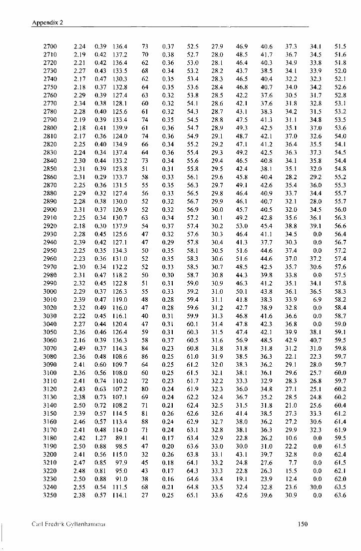
Appendix 2
2700 2.24 0.39 136.4 73 0.37 52.5 27.9 46.9 40.6 37.3 34.1 51.5 2710 2.19 0.42 137.2 70 0.38 52.7 28.0 48.5 41.7 36.7 34.5 51.6 2720 2.21 0.42 136.4 62 0.36 53.0 28.1 46.4 40.3 34.9 33.8 51.8 2730 2.27 0.43 133.5 68 0.34 53.2 28.2 43.7 38.5 34.1 33.9 52.0 2740 2.17 0.47 130.3 62 0.35 53.4 28.3 46.5 40.4 32.2 32.3 52.1 2750 2.18 0.37 132.8 64 0.35 53.6 28.4 46.8 40.7 34.0 34.2 52.6 2760 2.29 0.39 127.4 63 0.32 53.8 28.5 42.2 37.6 30.5 31.7 52.8 2770 2.34 0.38 128.1 60 0.32 54.1 28.6 42.1 37.6 31.8 32.8 53.1 2780 2.28 0.40 125.6 61 0.32 54.3 28.7 43.1 38.3 34.2 31.5 53.2 2790 2.19 0.39 133.4 74 0.35 54.5 28.8 47.5 41.3 31.1 34.8 53.5 2800 2.18 0.41 139.9 61 0.36 54.7 28.9 49.3 42.5 35.1 37.0 53.6 2810 2.17 0.36 124.0 74 0.36 54.9 29.1 48.7 42.1 37.0 32.6 54.0 2820 2.25 0.40 134.9 66 0.34 55.2 29.2 47.1 41.2 36.4 35.5 54.1 2830 2.24 0.34 137.4 64 0.36 55.4 29.3 49.2 42.5 36.3 37.3 54.5 2840 2.30 0.44 133.2 73 0.34 55.6 29.4 46.5 40.8 34.1 35.8 54.4 2850 2.31 0.39 123.8 51 0.31 55.8 29.5 42.4 38.1 35.1 32.0 54.8 2860 2.31 0.29 133.7 58 0.33 56.1 29.6 45.8 40.4 28.2 29.2 55.2 2870 2.25 0.36 131.5 55 0.35 56.3 29.7 49.1 42.6 35.4 36.0 55.3 2880 2.29 0.32 127.4 56 0.33 56.5 29.8 46.4 40.9 33.7 34.4 55.7 2890 2.28 0.38 130.0 52 0.32 56.7 29.9 46.1 40.7 32.1 28.0 55.7 2900 2.31 0.37 126.9 52 0.32 56.9 30.0 45.7 40.5 32.0 34.5 56.0 2910 2.25 0.34 130.7 63 0.34 57.2 30.1 49.2 42.8 35.6 36.1 56.3 2920 2.18 0.30 137.9 54 0.37 57.4 30.2 53.0 45.4 38.8 39.1 56.6 2930 2.28 0.45 125.6 47 0.32 57.6 30.3 46.4 41.1 34.5 0.0 56.4 2940 2.39 0.42 127.1 47 0.29 57.8 30.4 41.3 37.7 30.3 0.0 56.7 2950 2.25 0.35 134.3 50 0.35 58.1 30.5 51.6 44.6 37.4 0.0 57.2 2960 2.23 0.36 131.0 52 0.35 58.3 30.6 51.6 44.6 37.0 37.2 57.4 2970 2.30 0.34 132.2 52 0.33 58.5 30.7 48.5 42.5 35.7 30.6 57.6 2980 2.31 0.47 118.2 50 0.30 58.7 30.8 44.3 39.8 33.8 0.0 57.5 2990 2.32 0.45 122.8 51 0.31 59.0 30.9 46.3 41.2 35.1 34.1 57.8 3000 2.29 0.37 126.3 55 0.33 59.2 31.0 50.1 43.8 36.1 36.5 58.3 3010 2.39 0.47 119.0 48 0.28 59.4 31.1 41.8 38.3 33.9 6.9 58.2 3020 2.32 0.49 116.0 47 0.28 59.6 31.2 42.7 38.9 32.8 0.0 58.4 3030 2.22 0.45 116.1 40 0.31 59.9 31.3 46.8 41.6 36.6 0.0 58.7 3040 2.27 0.44 120.4 47 0.31 60.1 31.4 47.8 42.3 36.8 0.0 59.0 3050 2.36 0.46 126.4 59 0.31 60.3 31.5 47.4 42.1 39.9 38.1 59.1 3060 2.16 0.39 136.3 58 0.37 60.5 31.6 56.9 48.5 42.9 40.7 59.5 3070 2.49 0.37 114.3 84 0.23 60.8 31.8 31.8 31.8 31.2 31.0 59.8 3080 2.36 0.48 108.6 86 0.25 61.0 31.9 38.5 36.3 22.1 22.3 59.7 3090 2.41 0.60 109.7 64 0.25 61.2 32.0 38.3 36.2 29.1 28.0 59.7 3100 2.36 0.56 108.0 60 0.25 61.5 32.1 38.1 36.1 29.6 25.7 60.0 3110 2.41 0.74 110.2 72 0.23 61.7 32.2 33.3 32.9 28.3 26.8 59.7 3120 2.43 0.63 107.2 80 0.24 61.9 32.3 36.0 34.8 27.1 25.1 60.2 3130 2.38 0.73 107.1 69 0.24 62.2 32.4 36.7 35.2 28.5 24.8 60.2 3140 2.50 0.72 108.2 71 0.21 62.4 32.5 31.5 31.8 21.0 25.6 60.4 3150 2.39 0.57 114.5 81 0.26 62.6 32.6 41.4 38.5 27.3 33.3 61.2 3160 2.46 0.57 113.4 88 0.24 62.9 32.7 38.0 36.2 27.2 30.6 61.4 3170 2.41 0.48 114.0 71 0.24 63.1 32.8 38.1 36.3 29.9 32.3 61.9 3180 2.42 1.27 89.1 41 0.17 63.4 32.9 22.8 26.2 10.6 0.0 59.5 3190 2.50 0.88 98.5 47 0.20 63.6 33.0 30.0 31.0 22.2 0.0 61.5 3200 2.41 0.56 115.0 32 0.26 63.8 33.1 43.1 39.7 32.8 0.0 62.4 3210 2.47 0.85 97.9 45 0.18 64.1 33.2 24.8 27.6 7.7 0.0 61.5 3220 2.48 0.81 95.0 43 0.17 64.3 33.3 22.8 26.3 15.5 0.0 62.1 3230 2.50 0.88 91.0 38 0.16 64.6 33.4 19.1 23.9 12.4 0.0 62.0 3240 2.55 0.54 111.5 68 0.21 64.8 33.5 32.4 32.8 23.6 30.0 63.5 3250 2.38 0.57 114.1 27 0.25 65.1 33.6 42.6 39.6 30.9 0.0 63.6
Cur l F r e d r i k G y l l e n h a m i n u r 150

Appendix 2
3260 0.69 110.8 16 0.26 65.3 33.7 0.0 0.0 0.0 0.0 63.4 3270 2.49 1.01 96.7 31 0.18 65.5 33.8 27.4 29.5 29.6 0.0 62.7 3280 2.56 1.95 78.2 18 0.16 65.7 33.9 0.0 0.0 0.0 0.0 59.3 3290 2.36 0.75 75.0 9 0.23 66.0 34.0 0.0 0.0 0.0 0.0 63.9 3300 2.49 2.24 68.2 11 0.12 66.2 34.1 0.0 0.0 0.0 0.0 58.2 3310 2.46 1.90 68.7 10 0.13 66.4 34.2 0.0 0.0 0.0 0.0 59.8 3320 2.48 1.94 67.5 13 0.13 66.7 34.3 0.0 0.0 0.0 0.0 60.4 3330 2.46 1.70 67.4 9 0.16 66.9 34.5 0.0 0.0 0.0 0.0 61.3 3340 2.36 1.06 72.6 11 0.18 67.2 34.6 0.0 0.0 0.0 0.0 64.0 3350 2.44 1.36 72.5 11 0.19 67.4 34.7 0.0 0.0 0.0 0.0 63.4 3360 2.46 1.18 73.2 12 0.18 67.6 34.8 0.0 0.0 0.0 0.0 64.3 3370 2.36 0.75 71.6 9 0.20 67.9 34.9 0.0 0.0 0.0 0.0 65.9 3380 2.50 2.07 74.0 12 0.11 68.1 35.0 0.0 0.0 0.0 0.0 61.3 3390 2.62 6.07 62.2 13 0.04 68.4 35.1 0.0 0.0 0.0 0.0 44.3 3400 2.59 3.92 59.0 7 0.07 68.6 35.2 0.0 0.0 0.0 0.0 53.9 3410 2.48 1.52 62.2 6 0.10 68.9 35.3 0.0 0.0 0.0 0.0 64.2 3420 2.52 1.94 63.1 6 0.08 69.1 35.4 0.0 0.0 0.0 0.0 63.6 3430 2.46 0.86 67.2 7 0.14 69.3 35.5 0.0 0.0 0.0 0.0 67.0 3440 2.51 1.70 62.7 7 0.08 69.6 35.6 0.0 0.0 0.0 0.0 64.0 3450 2.51 1.63 60.9 6 0.08 69.8 35.7 0.0 0.0 0.0 0.0 65.1 3460 2.56 2.68 58.7 7 0.06 70.1 35.8 0.0 0.0 0.0 0.0 60.8 3470 2.52 1.43 65.2 7 0.10 70.3 35.9 0.0 0.0 0.0 0.0 66.3 3480 2.48 1.05 65.6 7 0.11 70.6 36.0 0.0 0.0 0.0 0.0 67.8 3490 2.53 2.85 59.3 6 0.06 70.8 36.1 0.0 0.0 0.0 0.0 58.4 3500 2.45 0.96 64.1 6 0.11 71.1 36.2 0.0 0.0 0.0 0.0 68.2 3510 2.61 5.46 55.0 6 0.04 71.3 36.3 0.0 0.0 0.0 0.0 50.5 3520 2.58 3.50 58.7 7 0.06 71.6 36.4 0.0 0.0 0.0 0.0 59.3 3530 2.43 0.78 69.2 6 0.15 71.8 36.5 0.0 0.0 0.0 0.0 69.3 3540 2.53 2.32 59.6 7 0.07 72.1 36.6 0.0 0.0 0.0 0.0 64.1 3550 2.56 2.43 62.1 7 0.08 72.3 36.7 0.0 0.0 0.0 0.0 63.5 3560 2.58 3.77 61.1 7 0.06 72.6 36.8 0.0 0.0 0.0 0.0 58.4 3570 2.58 3.59 57.0 6 0.05 72.8 36.9 0.0 0.0 0.0 0.0 59.0 3580 2.59 4.34 57.5 7 0.06 73.1 37.1 0.0 0.0 0.0 0.0 56.7 3590 2.55 2.58 60.8 7 0.07 73.3 37.2 0.0 0.0 0.0 0.0 65.0 3600 2.59 4.88 57.2 7 0.04 73.6 37.3 0.0 0.0 0.0 0.0 52.1 3610 2.60 3.96 58.1 7 0.05 73.8 37.4 0.0 0.0 0.0 0.0 58.7 3620 2.61 7.97 55.6 10 0.04 74.1 37.5 0.0 0.0 0.0 0.0 35.9 3630 2.62 7.03 55.7 7 0.03 74.4 37.6 0.0 0.0 0.0 0.0 41.4 3640 2.65 7.97 52.8 7 0.03 74.6 37.7 0.0 0.0 0.0 0.0 36.7 3650 2.64 10.01 55.4 9 0.03 74.9 37.8 0.0 0.0 0.0 0.0 17.8 3660 2.60 6.60 55.6 8 0.04 75.1 37.9 0.0 0.0 0.0 0.0 43.8 3670 2.57 4.04 65.9 13 0.09 75.4 38.0 0.0 0.0 0.0 0.0 59.6 3680 2.57 3.23 64.5 15 0.12 75.6 38.1 0.0 0.0 0.0 0.0 64.9 3690 2.50 2.65 68.1 12 0.13 75.9 38.2 0.0 0.0 0.0 0.0 66.6 3700 2.56 3.54 65.5 12 0.10 76.1 38.3 0.0 0.0 0.0 0.0 63.9 3710 2.56 3.40 67.4 12 0.10 76.4 38.4 0.0 0.0 0.0 0.0 63.7 3720 2.54 4.86 65.1 13 0.09 76.6 38.5 0.0 0.0 0.0 0.0 57.2 3730 2.60 5.06 62.5 10 0.08 76.9 38.6 0.0 0.0 0.0 0.0 56.1 3740 2.55 3.71 65.7 12 0.09 77.1 38.7 0.0 0.0 0.0 0.0 63.1 3750 2.51 2.74 66.8 11 0.12 77.4 38.8 0.0 0.0 0.0 0.0 68.5 3760 2.56 4.67 66.4 9 0.07 77.6 38.9 0.0 0.0 0.0 0.0 60.8 3770 2.59 5.47 62.5 14 0.06 77.9 39.0 0.0 0.0 0.0 0.0 54.1 3780 2.60 6.66 64.7 16 0.07 78.1 39.1 0.0 0.0 0.0 0.0 47.5 3790 2.61 6.46 62.7 16 0.06 78.4 39.2 0.0 0.0 0.0 0.0 49.9 3800 2.58 7.02 71.9 12 0.06 78.6 39.3 0.0 0.0 0.0 0.0 46.5 3810 2.62 7.18 65.2 12 0.05 78.9 39.4 0.0 0.0 0.0 0.0 46.0
C a r l F redr ik G y l l e n h a n i m n r 151

Appendix 2
3820 2.60 5.74 60.6 15 0.06 79.2 39.5 0.0 0.0 0.0 0.0 54.4 3830 2.60 5.76 64.1 15 0.08 79.4 39.6 0.0 0.0 0.0 0.0 55.3 3840 2.57 5.64 61.3 11 0.07 79.7 39.8 0.0 0.0 0.0 0.0 56.3 3850 2.55 5.35 63.2 12 0.09 79.9 39.9 0.0 0.0 0.0 0.0 57.4 3860 2.59 5.75 64.8 15 0.07 80.2 40.0 0.0 0.0 0.0 0.0 56.8 3870 2.61 6.21 62.6 17 0.07 80.4 40.1 0.0 0.0 0.0 0.0 54.6 3880 2.58 7.55 61.4 13 0.06 80.7 40.2 0.0 0.0 0.0 0.0 46.5 3890 2.59 7.63 61.6 15 0.07 80.9 40.3 0.0 0.0 0.0 0.0 47.0 3900 2.57 6.23 62.3 16 0.06 81.2 40.4 0.0 0.0 0.0 0.0 53.5 3910 2.62 7.18 60.1 16 0.06 81.4 40.5 0.0 0.0 0.0 0.0 49.4 3920 2.59 7.16 60.9 12 0.06 81.7 40.6 0.0 0.0 0.0 0.0 49.2 3930 2.60 10.57 58.2 10 0.04 81.9 40.7 0.0 0.0 0.0 0.0 23.4 3940 2.59 7.40 63.9 14 0.05 82.2 40.8 0.0 0.0 0.0 0.0 46.7 3950 2.60 5.79 68.8 15 0.06 82.5 40.9 0.0 0.0 0.0 0.0 55.7 3960 2.61 10.92 57.3 8 0.03 82.7 41.0 0.0 0.0 0.0 0.0 22.8 3970 2.56 5.08 57.9 8 0.08 83.0 41.1 0.0 0.0 0.0 0.0 63.6 3980 2.59 7.60 58.5 6 0.03 83.2 41.2 0.0 0.0 0.0 0.0 46.4 3990 2.56 4.57 57.2 7 0.07 83.5 41.3 0.0 0.0 0.0 0.0 67.0 4000 2.61 7.27 59.1 8 0.05 83.7 41.4 0.0 0.0 0.0 0.0 52.3 4010 2.60 7.01 65.4 9 0.04 84.0 41.5 0.0 0.0 0.0 0.0 53.6 4020 2.59 6.18 58.1 7 0.05 84.2 41.6 0.0 0.0 0.0 0.0 58.7 4030 2.61 11.22 56.9 8 0.03 84.5 41.7 0.0 0.0 0.0 0.0 25.5 4040 2.57 5.20 66.4 12 0.05 84.7 41.8 0.0 0.0 0.0 0.0 64.7 4050 2.63 10.63 56.5 11 0.03 85.0 41.9 0.0 0.0 0.0 0.0 29.8 4060 2.56 3.92 71.9 24 0.10 85.3 42.0 0.0 0.0 0.0 0.0 62.6 4070 2.61 8.47 60.6 16 0.06 85.5 42.1 0.0 0.0 0.0 0.0 48.0 4080 2.61 8.95 57.9 13 0.05 85.8 42.2 0.0 0.0 0.0 0.0 44.2 4090 2.61 4.27 61.4 17 0.08 86.0 42.3 0.0 0.0 0.0 0.0 71.2 4100 2.62 9.25 60.9 12 0.04 86.3 42.5 0.0 0.0 0.0 0.0 42.2 4110 2.60 5.57 57.9 8 0.06 86.5 42.6 0.0 0.0 0.0 0.0 64.5 4120 2.56 3.82 59.2 11 0.08 86.8 42.7 0.0 0.0 0.0 0.0 74.2 4130 2.59 4.64 60.6 14 0.07 87.0 42.8 0.0 0.0 0.0 0.0 71.5 4140 2.60 4.87 62.9 15 0.07 87.3 42.9 0.0 0.0 0.0 0.0 69.8 4150 2.56 3.46 69.1 24 0.13 87.5 43.0 0.0 0.0 0.0 0.0 77.1 4160 2.30 0.91 94.7 42 0.26 87.8 43.1 73.4 63.3 47.4 0.0 85.8 4170 2.57 3.95 62.3 11 0.08 88.0 43.2 0.0 0.0 0.0 0.0 74.6 4180 2.60 3.43 66.0 19 0.09 88.3 43.3 0.0 0.0 0.0 0.0 78.0 4190 2.60 3.83 63.1 17 0.09 88.6 43.4 0.0 0.0 0.0 0.0 75.8 4200 2.60 4.13 62.2 17 0.07 88.8 43.5 0.0 0.0 0.0 0.0 75.4 4210 2.62 3.52 64.4 18 0.08 89.1 43.6 0.0 0.0 0.0 0.0 78.6 4220 2.63 2.78 65.4 16 0.07 89.3 43.7 0.0 0.0 0.0 0.0 81.2 4230 2.56 1.60 66.3 15 0.12 89.6 43.8 0.0 0.0 0.0 0.0 85.6 4240 2.59 1.74 63.1 14 0.09 89.8 43.9 0.0 0.0 0.0 0.0 85.7 4250 2.57 2.23 64.4 14 0.10 90.1 44.0 0.0 0.0 0.0 0.0 84.5 4260 2.58 2.30 62.9 11 0.09 90.3 44.1 0.0 0.0 0.0 0.0 84.5 4270 2.52 3.03 66.0 15 0.09 90.6 44.2 0.0 0.0 0.0 0.0 82.7 4280 2.56 2.55 65.2 14 0.09 90.8 44.3 0.0 0.0 0.0 0.0 84.2 4290 2.58 3.09 67.2 14 0.09 91.1 44.4 0.0 0.0 0.0 0.0 83.0 4300 2.57 2.37 74.5 21 0.13 91.3 44.5 0.0 0.0 0.0 0.0 85.7 4310 2.56 1.22 84.7 37 0.14 91.6 44.6 48.6 47.2 32.9 0.0 88.8 4320 2.57 0.72 84.7 46 0.13 91.8 44.7 46.3 45.7 36.8 0.0 90.5 4330 2.60 0.91 84.8 49 0.12 92.1 44.8 42.9 43.6 25.8 0.0 90.2 4340 0.60 84.8 19 0.00 92.3 44.9 0.0 0.0 0.0 0.0 91.2 4350 0.75 114.0 25 0.09 92.5 45.1 0.0 0.0 0.0 0.0 91.1 4360 2.41 0.48 116.2 29 0.21 92.7 45.2 68.6 60.8 34.8 0.0 91.7 4370 2.26 2.84 98.6 29 0.30 93.0 45.3 87.0 73.1 55.5 0.0 86.5
Cal l F iec l i ik G y l l e n h a i n m a i ' 152
Appendix 2
4380 2.38 2.47 98.1 25 0.24 93.2 45.4 75.7 65.6 56.0 0.0 87.6 4390 2.27 3.03 102.1 27 0.30 93.4 45.5 87.8 73.7 64.7 0.0 85.7 4400 2.48 1.19 101.5 45 0.19 93.7 45.6 64.6 58.2 51.6 0.0 91.3 4410 2.35 1.09 134.9 100 0.25 93.9 45.7 79.9 68.5 58.0 74.4 91.7 4420 2.42 0.69 125.9 104 0.22 94.1 45.8 71.9 63.2 57.8 71.6 92.8 4430 2.37 0.68 131.8 120 0.24 94.4 45.9 76.7 66.4 53.0 74.2 93.1 4440 2.39 0.80 130.7 125 0.24 94.6 46.0 76.9 66.6 59.5 74.2 93.1 4450 2.54 0.89 114.6 73 0.17 94.8 46.1 60.6 55.7 57.1 65.3 93.2 4460 2.40 0.73 115.4 68 0.22 95.1 46.2 74.9 65.3 54.7 66.7 93.8 4470 2.30 1.41 137.5 93 0.25 95.3 46.3 81.0 69.4 67.2 76.9 92.3 4480 2.27 1.63 137.2 120 0.31 95.5 46.4 93.0 77.5 71.9 78.0 91.9 4490 2.33 1.14 133.9 116 0.24 95.8 46.5 79.4 68.4 66.7 76.4 93.4 4500 2.24 8.17 129.3 103 0.32 96.0 46.6 94.9 78.8 71.0 75.1 64.9 4510 2.22 25.31 117.9 95 0.33 96.2 46.7 96.7 80.0 73.5 71.1 -82.4 4520 2.33 0.59 123.7 70 0.26 96.4 46.8 85.2 72.4 67.3 72.9 95.3 4530 2.24 9.72 122.1 95 0.31 96.7 46.9 94.9 78.9 73.5 72.4 58.3 4540 2.19 0.65 139.5 72 0.34 96.9 47.0 100.0 82.3 71.5 80.3 95.6 4550 2.32 0.59 122.8 68 0.28 97.1 47.1 89.5 75.4 66.9 73.5 96.1 4560 2.34 0.57 130.3 72 0.27 97.3 47.2 86.9 73.6 66.2 76.9 96.3 4570 2.37 0.56 121.3 67 0.24 97.6 47.3 81.7 70.3 61.5 73.5 96.6 4580 2.34 0.64 125.7 78 0.26 97.8 47.4 85.5 72.8 61.2 75.4 96.6 4590 2.32 1.33 129.7 87 0.27 98.0 47.5 88.1 74.6 67.0 77.5 95.2 4600 2.21 3.70 126.8 93 0.33 98.3 47.6 99.2 82.0 75.3 77.2 88.3 4610 2.28 0.50 143.1 103 0.31 98.5 47.8 95.7 79.7 71.9 82.8 97.7 4620 2.26 1.06 144.4 101 0.30 98.7 47.9 95.7 79.7 74.9 83.5 96.9 4630 2.30 0.58 142.9 107 0.28 98.9 48.0 92.1 77.4 70.3 83.3 98.0 4640 2.30 0.55 137.3 108 0.29 99.2 48.1 92.9 78.0 70.5 82.0 98.3 4650 2.35 0.31 134.3 107 0.27 99.4 48.2 89.5 75.7 68.9 81.5 98.9 4660 2.49 0.41 105.8 76 0.22 99.6 48.3 80.3 69.6 66.1 66.1 99.0 4670 2.33 0.31 126.7 82 0.27 99.9 48.4 91.4 77.1 68.6 79.3 99.3 4680 2.39 0.35 114.8 68 0.24 100.1 48.5 84.2 72.3 65.8 72.7 99.5 4690 2.41 0.35 107.5 68 0.22 100.3 48.6 80.7 70.0 62.5 67.3 99.8 4700 2.40 0.37 108.0 69 0.24 100.6 48.7 84.9 72.8 65.8 68.4 100.0 4710 2.39 0.41 107.5 70 0.24 100.8 48.8 85.4 73.2 65.4 67.1 100.1 4720 2.43 0.37 105.9 74 0.21 101.0 48.9 79.8 69.5 60.2 66.5 100.4 4730 2.40 0.36 108.9 76 0.23 101.3 49.0 85.0 73.0 63.2 69.7 100.7 4740 2.40 0.40 107.9 75 0.24 101.5 49.1 86.3 73.9 65.4 69.7 100.9 4750 2.44 0.66 89.6 63 0.18 101.7 49.2 71.8 64.3 64.4 44.7 100.7 4760 2.39 0.49 97.4 59 0.19 102.0 49.3 76.3 67.3 59.3 59.9 101.2 4770 2.40 0.41 99.1 69 0.20 102.2 49.4 78.9 69.1 61.6 60.9 101.6 4780 2.41 0.42 98.1 60 0.19 102.4 49.5 76.0 67.2 58.4 60.5 101.8 4790 2.42 0.37 102.8 72 0.22 102.7 49.6 84.0 72.5 65.3 65.6 102.1 4800 2.42 0.38 100.4 70 0.22 102.9 49.7 85.0 73.2 64.1 63.2 102.3 4810 2.46 0.42 95.7 69 0.20 103.1 49.8 80.1 70.0 62.3 58.1 102.5 4820 2.42 0.34 108.0 77 0.22 103.4 49.9 85.4 73.6 63.9 70.9 102.9 4830 2.45 0.59 90.0 70 0.20 103.6 50.0 80.4 70.3 58.4 55.7 102.8 4840 2.43 0.41 96.6 70 0.21 103.9 50.1 82.7 71.8 62.8 61.0 103.2 4850 2.44 0.46 96.7 67 0.20 104.1 50.2 81.9 71.3 63.1 60.6 103.4 4860 2.46 0.44 97.9 69 0.20 104.3 50.4 80.9 70.7 62.3 62.7 103.7 4870 2.46 0.43 102.0 74 0.20 104.6 50.5 80.1 70.2 61.5 67.6 103.9 4880 2.36 1.02 80.6 36 0.17 104.8 50.6 74.3 66.4 63.4 14.7 103.5 4890 2.27 0.27 89.9 28 0.21 105.0 50.7 83.7 72.7 64.6 0.0 104.6 4900 2.26 0.35 90.6 28 0.21 105.3 50.8 85.1 73.6 65.4 0.0 104.8 4910 2.30 0.43 98.1 37 0.21 105.5 50.9 84.4 73.2 66.3 0.0 104.9 4920 2.35 0.43 87.7 29 0.20 105.7 51.0 83.7 72.8 65.0 0.0 105.1 4930 2.28 0.30 91.0 26 0.20 105.9 51.1 83.6 72.7 62.1 0.0 105.5
Car l F redr ik G y l l e n h a m m a r 153

Appendix 2
4940 2.31 0.54 89.1 30 0.20 106.2 51.2 82.8 72.3 64.6 0.0 105.4 4950 2.27 0.38 87.6 31 0.20 106.4 51.3 84.8 73.6 62.1 0.0 105.8 4960 2.29 0.39 87.3 27 0.20 106.6 51.4 82.9 72.4 66.0 0.0 106.0 4970 2.25 0.35 86.0 21 0.21 106.8 51.5 0.0 0.0 0.0 0.0 106.3 4980 2.46 0.52 88.8 66 0.19 107.1 51.6 81.6 71.6 61.5 51.4 106.3 4990 2.52 0.51 87.2 74 0.15 107.3 51.7 72.8 65.7 54.7 51.5 106.6
Car l F i ed i ik G y l l e n h a m m a i - 154

Appendix 3
Appendix 3 The following table are the calculated pore pressure values used in Figure 3.19. Due to the fact that this study was based on a Gulf of Mexico well the pressure are measured in psi. 1 megaPascal (MPa) is equal 145 psi.
Depth, measured Eaton PresGraf EQVD EQVD Eaton/EQVD PresG/EQ Water Depth=975 PresGraf normal trend Conoco Normal trend
Pressure Pressure Pressure Pressure feet meters (psi) (psi) (psi) (psi) 2715 827.5421 944.502 994.62 1287 0.949611 0.772821 2770 844.3063 938.738 993.986 1298 0.944418 0.765783 2786 849.1831 926.068 985.069 1308 0.940105 0.753111 2807 855.584 913.98 976.99 1322 0.935506 0.739024 2854 869.9098 919.338 985.123 1353 0.933222 0.728103 2868 874.177 929.203 993.481 1340 0.9353 0.741404 2894 882.1019 938.58 1003 1357 0.935773 0.73913 2920 890.0268 942.417 1008 1373 0.934938 0.734159 2966 904.0478 953.333 1021 1402 0.933725 0.728245 2976 907.0958 969.038 1034 1409 0.937174 0.733854 3008 916.8495 999.899 1061 1409 0.942412 0.753016 3035 925.0792 1035 1093 1426 0.946935 0.76648 3092 942.4531 1072 1127 1462 0.951198 0.770862 3098 944.2819 1083 1136 1466 0.953345 0.774898 3140 957.0836 1157 1200 1472 0.964167 0.815217 3173 967.1422 1199 1237 1493 0.969281 0.828533 3177 968.3614 1192 1232 1495 0.967532 0.82408 3228 983.9064 1250 1283 1527 0.974279 0.84021 3258 993.0505 1309 1334 1525 0.981259 0.874754 3261 993.9649 1310 1336 1527 0.980539 0.874918 3305 1007.376 1335 1360 1554 0.981618 0.875161 3336 1016.825 1311 1342 1572 0.9769 0.85369 3361 1024.445 1353 1379 1587 0.981146 0.868935 3423 1043.343 1294 1334 1607 0.970015 0.830118 3470 1057.669 1301 1343 1636 0.968727 0.820905 3487 1062.851 1331 1369 1647 0.972243 0.831208 3522 1073.519 1288 1335 1647 0.964794 0.810565 3552 1082.663 1335 1377 1666 0.969499 0.826531 3561 1085.406 1352 1392 1672 0.971264 0.832536 3605 1098.817 1411 1444 1699 0.977147 0.849912 3612 1100.951 1414 1447 1703 0.977194 0.849677 3639 1109.181 1428 1461 1720 0.977413 0.849419 3714 1132.041 1504 1530 1745 0.983007 0.876791 3785 1153.682 1550 1574 1790 0.984752 0.87933 3838 1169.837 1601 1620 1799 0.988272 0.9005 3874 1180.81 1586 1610 1822 0.985093 0.883644 3988 1215.557 1581 1613 1870 0.980161 0.862567 4092 1247.257 1785 1794 1933 0.994983 0.928091 4199 1279.871 1941 1935 2028 1.003101 0.954142 4227 1288.405 2006 1992 2104 1.007028 0.946768
Car l F red r ik G y l l e n h a m m a r 155
Appendix 3
4274 1302.731 2092 2069 2216 1 .011116 0.933664 4302 1311.266 2188 2154 2320 1 .015785 0.928448 4331 1320.105 2261 2219 2409 1 .018927 0.921129 4356 1327.725 2321 2272 2485 1 .021567 0.914286 4372 1332.602 2349 2297 2516 1 .022638 0.912957 4416 1346.013 2442 2380 2614 1 .02605 0.910482 4449 1356.072 2489 2423 2674 1 .027239 0.906133 4477 1364.606 2474 2413 2648 1 .02528 0.911254 4526 1379.542 2483 2424 2654 1 .02434 0.913338 4572 1393.563 2453 2402 2606 1 .021232 0.921719 4577 1395.087 2451 2401 2602 1 .020825 0.922752 4605 1403.621 2460 2410 2592 1 .020747 0.929784 4636 1413.07 2502 2449 2643 1 .021641 0.926599 4672 1424.043 2529 2475 2653 1 .021818 0.932906 4696 1431.358 2540 2486 2673 1 .021722 0.930041 4734 1442.941 2577 2521 2708 1 .022213 0.930945 4815 1467.63 2680 2617 2828 1 .024073 0.925389 4864 1482.565 2860 2777 3056 516.408 1 .029888 0.908704 4892 1491.1 2922 2833 3134 675.434 1 .031415 0.903957 4911 1496.891 2959 2867 3164 766.058 1 .032089 0.906131 4930 1502.682 2977 2884 3181 792.8 1 .032247 0.906633 4973 1515.789 3080 2978 3319 1068 1 .034251 0.897258 5008 1526.457 3145 3037 3401 1222 1 .035561 0.892973 5013 1527.981 3106 3003 3340 1080 1 .034299 0.899102 5367 1635.881 3249 3157 3395 917.142 1 .029142 0.929897 5517 1681.602 3353 3260 3502 993.994 1 .028528 0.930897 5767 1757.803 3542 3446 3680 1154 1 .027858 0.936413 5804 1769.081 3546 3452 3665 1100 1 .027231 0.941883 5834 1778.225 3575 3481 3693 1140 1 .027004 0.942594 5890 1795.294 3667 3566 3808 1332 1 .028323 0.93645 5909 1801.085 3713 3609 3857 1455 1 028817 0.935701 5940 1810.534 3760 3653 3912 1548 1 .029291 0.933793 5967 1818.764 3804 3695 3963 1641 1 .029499 0.932374 6004 1830.041 3844 3733 4006 1701 1 .029735 0.931852 6007 1830.956 3841 3730 4002 1687 1 029759 0.932034 6042 1841.624 3853 3743 4008 1660 1 029388 0.933882 6083 1854.121 3883 3773 4042 1682 1 .029155 0.933449 6112 1862.96 3916 3806 4063 1742 1 028902 0.936746 6135 1869.971 3943 3831 4092 1786 1 029235 0.936217 6160 1877.591 3963 3851 4114 1804 1 029083 0.936072 6184 1884.906 3986 3874 4137 1835 1 028911 0.936427 6221 1896.184 4026 3912 4172 1896 1 .029141 0.93768 6269 1910.814 4082 3965 4241 1985 1 .029508 0.934921 6280 1914.167 4094 3976 4254 2003 1 029678 0.93465 6306 1922.092 4125 4008 4273 2062 1 029192 0.937983 6336 1931.236 4157 4038 4309 2110 1 02947 0.937108 6376 1943.428 4187 4068 4340 2133 1 029253 0.937327 6388 1947.086 4183 4066 4326 2099 1 028775 0.939898 6425 1958.364 4214 4096 4361 2128 1 028809 0.939234 6455 1967.508 4213 4097 4353 2071 1 028313 0.94119
Car l l - redr ik G y l l e n h a i m n a r 156
Appendix 3
6480 1975.128 4204 4091 4338 2001 1 .027622 0.943061 6522 1987.93 4234 4122 4349 2025 1 .027171 0.947804 6530 1990.368 4234 4122 4335 2012 1 .027171 0.950865 6585 2007.132 4250 4140 4353 1963 1 .02657 0.951068 6612 2015.362 4247 4140 4342 1908 1 .025845 0.953478 6647 2026.03 4206 4106 4282 1718 1 .024355 0.958898 6658 2029.383 4206 4107 4279 1698 1 .024105 0.959804 6687 2038.222 4163 4069 4213 1510 1 .023101 0.96582 6708 2044.623 4157 4066 4222 1455 1 .022381 0.963051 6739 2054.072 4167 4078 4211 1440 1 .021824 0.968416 6771 2063.826 4180 4092 4230 1423 1 .021505 0.967376 6789 2069.312 4201 4112 4248 1453 1 .021644 0.967985 6817 2077.847 4233 4143 4273 1503 1 .021723 0.969576 6845 2086.381 4253 4163 4300 1514 1 .021619 0.96814 6996 2132.407 4309 4224 4348 1429 1 .020123 0.971481 7019 2139.417 4323 4239 4359 1433 1 .019816 0.972471 7036 2144.599 4297 4216 4339 1323 1 .019213 0.971652 7071 2155.267 4317 4236 4358 1322 1 .019122 0.972006 7086 2159.839 4321 4241 4360 1309 1 .018863 0.972706 7119 2169.898 4397 4312 4430 1482 1 .019712 0.973363 7163 2183.309 4512 4421 4541 1762 1 .020584 0.973574 7180 2188.491 4554 4460 4591 1858 1 .021076 0.971466 7213 2198.549 4641 4541 4682 2062 1 .022022 0.969885 7247 2208.912 4735 4629 4784 2286 1 .022899 0.9676 7292 2222.629 4810 4700 4862 2431 1 .023404 0.96668 7294 2223.238 4810 4701 4864 2430 1 .023187 0.966488 7337 2236.345 4863 4751 4907 2512 1 023574 0.968209 7351 2240.612 4842 4733 4896 2427 1 02303 0.966708 7392 2253.109 4889 4780 4932 2504 1 022803 0.969181 7420 2261.644 4889 4783 4924 2457 1 .022162 0.971365 7440 2267.74 4888 4783 4930 2418 1 .021953 0.970183 7480 2279.932 4832 4734 4852 2182 1 .020701 0.97568 7489 2282.675 4806 4712 4840 2090 1 019949 0.973554 7524 2293.343 4805 4713 4825 2028 1 01952 0.976788 7565 2305.84 4850 4757 4881 2093 1 01955 0.974595 7589 2313.155 4860 4767 4890 2081 1 019509 0.974847 7626 2324.433 4880 4790 4899 2088 1 018789 0.977751 7663 2335.711 4952 4858 4960 2240 1 01935 0.979435 7681 2341.197 5022 4923 5046 2415 1 02011 0.975624 7699 2346.684 5049 4948 5064 2464 1 020412 0.977093 7727 2355.218 5074 4973 5092 2490 1 02031 0.97663 7765 2366.801 5132 5029 5163 2601 1 020481 0.974046 7804 2378.688 5198 5092 5231 2732 1 020817 0.973428 7814 2381.736 5208 5102 5240 2744 1 020776 0.973664 7839 2389.356 5231 5126 5255 2780 1 020484 0.975452 7876 2400.634 5261 5156 5284 2808 1 020365 0.975776 7922 2414.655 5329 5221 5342 2931 1 020686 0.977349 7936 2418.922 5353 5244 5375 2979 1 020786 0.975628 7988 2434.772 5406 5296 5430 3049 1 02077 0.975322 8012 2442.087 5419 5310 5442 3048 1 020527 0.975744
C a r l F redr ik G y l l e n h a m m a r 157

Appendix 3
8040 2450.622 5431 5323 5455 3036 1 .020289 0.975802 8067 2458.851 5448 5340 5475 3041 1 .020225 0.975342 8084 2464.033 5471 5364 5486 3089 1 .019948 0.977762 8126 2476.835 5504 5397 5519 3114 1 .019826 0.977895 8139 2480.797 5504 5398 5517 3092 1 .019637 0.97843 8188 2495.733 5559 5452 5575 3172 1 .019626 0.977937 8215 2503.962 5591 5483 5609 3219 1 .019697 0.977536 8217 2504.572 5591 5483 5607 3217 1 .019697 0.977885 8250 2514.631 5548 5447 5557 3039 1 .018542 0.980205 8298 2529.261 5544 5447 5555 2949 1 .017808 0.980558 8370 2551.207 5471 5387 5466 2631 1 .015593 0.985547 8375 2552.731 5493 5407 5490 2685 1 .015905 0.984882 8419 2566.142 5513 5428 5504 2669 1 .01566 0.986192 8450 2575.591 5489 5408 5487 2549 1 .014978 0.985602 8456 2577.42 5489 5409 5487 2541 1 .01479 0.985785 8492 2588.393 5463 5387 5462 2408 1 .014108 0.986269 8518 2596.318 5485 5410 5486 2430 1 .013863 0.986147 8578 2614.606 5525 5452 5507 2457 1 .01339 0.990013 8607 2623.446 5557 5483 5543 2501 1 .013496 0.989176 8635 2631.98 5613 5537 5601 2614 1 .013726 0.988573 8689 2648.439 5681 5603 5668 2718 1 .013921 0.988532 8719 2657.584 5699 5622 5692 2722 1 .013696 0.987702 8737 2663.07 5713 5636 5703 2731 1 .013662 0.988252 8763 2670.995 5719 5644 5710 2707 1 .013288 0.988441 8794 2680.444 5717 5644 5709 2652 1 .012934 0.988614 8813 2686.235 5742 5670 5709 2703 1 .012698 0.993169 8843 2695.379 5814 5738 5791 2855 1 .013245 0.990848 8867 2702.694 5832 5757 5811 2869 1 .013028 0.990707 8912 2716.411 5851 5777 5830 2848 1 .012809 0.990909 8917 2717.935 5856 5783 5833 2856 1 .012623 0.991428 8966 2732.87 5896 5823 5864 2889 1 .012536 0.993008 8990 2740.185 5894 5823 5876 2844 1 .012193 0.99098 9032 2752.987 5868 5802 5843 2706 1 .011375 0.992983 9056 2760.302 5892 5826 5870 2735 1 .011329 0.992504 9083 2768.532 5927 5862 5895 2801 1 .011088 0.994402 9113 2777.676 5961 5895 5925 2847 1 .011196 0.994937 9137 2784.991 5967 5903 5937 2828 1 .010842 0.994273 9179 2797.793 6000 5936 5968 2852 1 .010782 0.994638 9199 2803.889 6019 5955 5989 2873 1 .010747 0.994323 9230 2813.338 6053 5989 6027 2920 1 .010686 0.993695 9249 2819.129 6055 5991 6025 2894 1 .010683 0.994357 9279 2828.274 6104 6039 6077 2983 1 .010763 0.993747 9312 2838.332 6150 6084 6125 3060 1 .010848 0.993306 9335 2845.343 6173 6109 6132 3098 1 .010476 0.996249 9384 2860.278 6265 6198 6224 3274 1 .01081 0.995823 9416 2870.032 6310 6241 6270 3348 1 .011056 0.995375 9476 2888.32 6321 6256 6287 3285 1 .01039 0.995069 9500 2895.635 6365 6299 6320 3369 1 .010478 0.996677 9508 2898.074 6325 6262 6289 3248 1 .010061 0.995707 9538 2907.218 6281 6224 6246 3083 1 .009158 0.996478
Car! F i e d r i k G y l l e n h a m m a r 158
Appendix 3
9563 2914.838 6284 6228 6251 3053 1.008992 0.996321 9601 2926.42 6262 6212 6215 2946 1.008049 0.999517 9624 2933.431 6297 6246 6249 3006 1.008165 0.99952 9651 2941.661 6277 6230 6229 2913 1.007544 1.000161 9673 2948.366 6308 6260 6262 2964 1.007668 0.999681 9718 2962.082 6445 6390 6397 3265 1.008607 0.998906 9772 2978.542 6653 6587 6596 3746 1.01002 0.998636 9803 2987.991 6790 6717 6752 4071 1.010868 0.994816 9848 3001.707 7020 6933 6975 4629 1.012549 0.993978 9872 3009.022 7084 6995 7038 4767 1.012723 0.99389 9885 3012.985 7102 7012 7056 4793 1.012835 0.993764 9936 3028.53 7198 7104 7151 4974 1.013232 0.993427 9960 3035.845 7300 7200 7265 5211 1.013889 0.991053 9973 3039.807 7307 7207 7270 5209 1.013875 0.991334 9995 3046.513 7337 7237 7302 5259 1.013818 0.991098 10036 3059.01 7429 7325 7401 5444 1.014198 0.989731 10086 3074.25 7493 7387 7472 5540 1.01435 0.988624 10109 3081.261 7498 7395 7450 5524 1.013928 0.992617 10123 3085.528 7484 7384 7443 5468 1.013543 0.992073 10160 3096.806 7492 7395 7436 5433 1.013117 0.994486 10191 3106.255 7505 7409 7463 5423 1.012957 0.992764 10213 3112.96 7503 7410 7458 5387 1.012551 0.993564 10247 3123.324 7503 7413 7456 5337 1.012141 0.994233 10262 3127.896 7507 7418 7462 5326 1.011998 0.994103 10291 3136.735 7526 7437 7478 5333 1.011967 0.994517 10344 3152.89 7556 7470 7503 5335 1.011513 0.995602 10371 3161.119 7613 7524 7567 5444 1.011829 0.994317 10385 3165.386 7646 7557 7593 5518 1.011777 0.995259 10439 3181.846 7716 7626 7656 5623 1.011802 0.996082 10456 3187.028 7752 7661 7697 5694 1.011878 0.995323 10494 3198.61 7814 7721 7765 5800 1.012045 0.994334 10515 3205.011 7841 7748 7785 5840 1.012003 0.995247 10547 3214.765 7885 7791 7831 5909 1.012065 0.994892 10581 3225.128 7927 7832 7876 5969 1.01213 0.994413 10605 3232.443 7955 7860 7908 6010 1.012087 0.99393 10625 3238.539 7982 7886 7937 6050 1.012173 0.993574 10650 3246.159 8008 7912 7962 6083 1.012133 0.99372 10693 3259.266 8059 7965 8003 6162 1.011802 0.995252 10698 3260.79 8066 7971 8013 6172 1.011918 0.994759 10876 3315.045 8458 8345 8441 6938 1.013541 0.988627 10953 3338.515 8548 8436 8538 7065 1.013276 0.988053 10985 3348.269 8585 8473 8580 7116 1.013218 0.987529 10995 3351.317 8587 8476 8578 7108 1.013096 0.988109 11071 3374.482 8629 8521 8609 7109 1.012675 0.989778 11139 3395.208 8661 8556 8629 7094 1.012272 0.99154 11145 3397.037 8651 8548 8612 7060 1.01205 0.992569 11176 3406.486 8669 8567 8627 7062 1.011906 0.993045 11200 3413.802 8671 8572 8629 7034 1.011549 0.993394 11250 3429.042 8693 8598 8627 7025 1.011049 0.996638 11273 3436.052 8713 8620 8649 7046 1.010789 0.996647
Car l Fredr ik G y l l e n h a m m a r 159

Appendix 3
11305 3445.806 8710 8620 8646 6992 1.010441 0.996993 11326 3452.207 8711 8623 8637 6967 1.010205 0.998379 11362 3463.18 8733 8647 8667 6972 1.009946 0.997692 11386 3470.495 8765 8678 8696 7020 1.010025 0.99793 11446 3488.783 8790 8707 8718 7000 1.009533 0.998738 11492 3502.804 8804 8724 8731 6969 1.00917 0.999198 11518 3510.729 8834 8756 8752 7015 1.008908 1.000457 11521 3511.644 8817 8741 8729 6968 1.008695 1.001375 11591 3532.98 8858 8785 8772 6975 1.00831 1.001482 11605 3537.247 8867 8795 8782 6979 1.008186 1.00148 11637 3547.001 8908 8835 8823 7037 1.008263 1.00136 11681 3560.412 8914 8846 8824 6991 1.007687 1.002493 11716 3571.08 8949 8881 8858 7031 1.007657 1.002597 11717 3571.385 8951 8883 8862 7035 1.007655 1.00237 11783 3591.502 8999 8933 8901 7063 1.007388 1.003595 11815 3601.256 9003 8943 8900 7036 1.006709 1.004831 11924 3634.479 9104 9046 9001 7139 1.006412 1.004999 11934 3637.527 9109 9052 9008 7138 1.006297 1.004885 11974 3649.72 9141 9084 9027 7161 1.006275 1.006314 11983 3652.463 9149 9093 9036 7169 1.006159 1.006308 12031 3667.093 9160 9108 9060 7130 1.005709 1.005298 12065 3677.457 9187 9136 9087 7151 1.005582 1.005392 12072 3679.59 9138 9092 9034 7019 1.005059 1.00642 12100 3688.125 9107 9070 8985 6913 1.004079 1.00946 12148 3702.755 9143 9108 9018 6936 1.003843 1.00998 12168 3708.851 9244 9202 9132 7157 1.004564 1.007665 12216 3723.482 9344 9297 9234 7335 1.005055 1.006823 12248 3733.236 9457 9403 9354 7569 1.005743 1.005238 12270 3739.941 9532 9473 9434 7722 1.006228 1.004134 12304 3750.305 9563 9504 9465 7751 1.006208 1.00412 12310 3752.134 9556 9499 9456 7727 1.006001 1.004547 12353 3765.24 9596 9540 9486 7766 1.00587 1.005693 12370 3770.422 9616 9560 9518 7791 1.005858 1.004413 12389 3776.213 9624 9569 9525 7785 1.005748 1.004619 12420 3785.662 9662 9610 9556 7844 1.005411 1.005651 12472 3801.512 9727 9674 9609 7931 1.005479 1.006764 12494 3808.218 9763 9708 9659 7988 1.005665 1.005073 12518 3815.533 9781 9728 9676 8001 1.005448 1.005374 12557 3827.42 9799 9748 9698 7991 1.005232 1.005156 12571 3831.687 9775 9728 9666 7915 1.004831 1.006414 12610 3843.575 9792 9748 9685 7903 1.004514 1.006505 12654 3856.986 9771 9734 9656 7793 1.003801 1.008078 12655 3857.291 9748 9714 9637 7738 1.0035 1.00799 12705 3872.531 9773 9745 9631 7738 1.002873 1.011837 12711 3874.36 9765 9738 9638 7711 1.002773 1.010376 12742 3883.809 9754 9732 9623 7644 1.002261 1.011327 12767 3891.429 9727 9710 9592 7546 1.001751 1.012302 12815 3906.059 9721 9710 9584 7469 1.001133 1.013147 12823 3908.498 9708 9699 9569 7428 1.000928 1.013586 12883 3926.786 9753 9746 9614 7456 1.000718 1.01373
Gai l F redr ik G y l l e n h a m m a i 160

Appendix 3
12900 3931.968 9785 9778 9650 7511 1.000716 1.013264 12940 3944.16 9820 9814 9685 7542 1.000611 1.01332 12959 3949.951 9849 9842 9715 7588 1.000711 1.013073 12984 3957.571 9880 9873 9747 7630 1.000709 1.012927 13011 3965.801 9890 9888 9744 7628 1.000202 1.014778 13033 3972.507 9894 9894 9746 7610 1 1.015186 13068 3983.175 9900 9903 9755 7578 0.999697 1.015172 13099 3992.624 9926 9930 9783 7601 0.999597 1.015026 13144 4006.34 9961 9967 9818 7627 0.999398 1.015176 13199 4023.104 10055 10059 9898 7781 0.999602 1.016266 13235 4034.077 10131 10131 9993 7914 1 1.01381 13243 4036.515 10146 10146 10009 7940 1 1.013688 13296 4052.67 10240 10237 10102 8091 1.000293 1.013364 13322 4060.595 10287 10285 10141 8177 1.000194 1.0142 13342 4066.691 10304 10302 10159 8191 1.000194 1.014076 13375 4076.75 10337 10336 10193 8227 1.000097 1.014029 13384 4079.493 10343 10343 10199 8229 1 1.014119 13415 4088.942 10387 10386 10246 8292 1.000096 1.013664 13462 4103.267 10443 10443 10303 8364 1 1.013588 13476 4107.535 10467 10466 10330 8401 1.000096 1.013166 13507 4116.984 10503 10502 10366 8446 1.000095 1.01312 13545 4128.566 10548 10547 10414 8503 1.000095 1.012771 13572 4136.796 10563 10563 10426 8503 1 1.01314 13616 4150.207 10603 10605 10468 8542 0.999811 1.013088 13643 4158.437 10639 10643 10494 8600 0.999624 1.014199 13649 4160.266 10641 10646 10495 8596 0.99953 1.014388 13701 4176.116 10615 10629 10466 8471 0.998683 1.015574 13715 4180.383 10591 10609 10441 8398 0.998303 1.01609 13815 4210.863 10475 10515 10315 8004 0.996196 1.019389 13817 4211.473 10468 10509 10309 7987 0.996099 1.019401 13851 4221.836 10402 10453 10242 7792 0.995121 1.020601 13887 4232.809 10321 10383 10153 7561 0.994029 1.022653 13942 4249.573 10314 10382 10152 7476 0.99345 1.022656 13947 4251.097 10308 10377 10144 7456 0.993351 1.022969 13989 4263.899 10293 10370 10118 7381 0.992575 1.024906 14001 4267.557 10298 10376 10123 7378 0.992483 1.024993 14049 4282.187 10380 10457 10199 7507 0.992637 1.025297 14057 4284.626 10406 10482 10209 7557 0.992749 1.026741 14110 4300.78 10514 10587 10343 7741 0.993105 1.023591 14111 4301.085 10515 10588 10344 7741 0.993105 1.023589 14152 4313.582 10573 10646 10403 7822 0.993143 1.023359 14177 4321.202 10594 10668 10425 7840 0.993063 1.023309 14216 4333.089 10660 10733 10486 7945 0.993199 1.023555 14242 4341.014 10684 10758 10516 7967 0.993121 1.023013 14274 4350.768 10797 10865 10638 8187 0.993741 1.021339 14299 4358.388 10847 10916 10674 8281 0.993679 1.022672 14399 4388.869 10931 11004 10760 8351 0.993366 1.022677 14412 4392.831 10901 10979 10732 8269 0.992896 1.023015 14457 4406.547 10861 10946 10694 8122 0.992235 1.023565 14484 4414.777 10843 10933 10669 8051 0.991768 1.024745
Car l Fredr ik ( j y l l e n h a m m a r 161
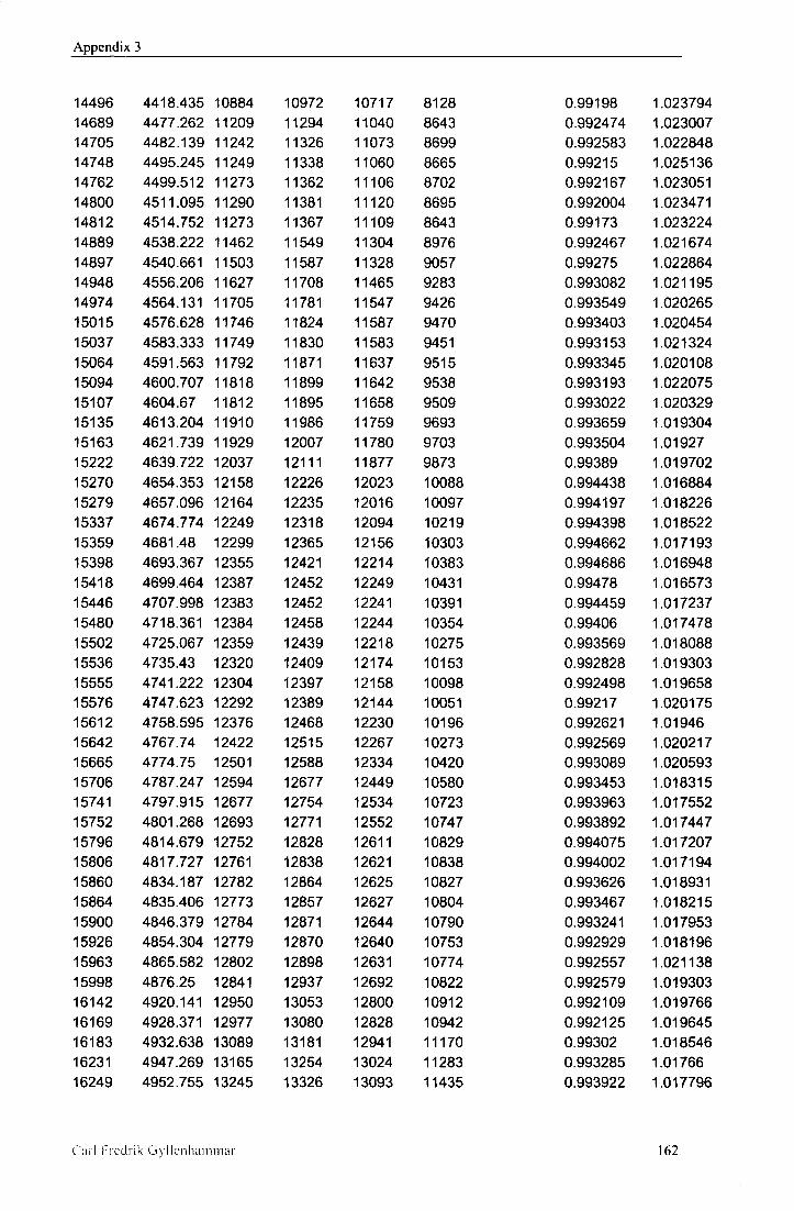
Appendix 3
14496 4418.435 10884 10972 10717 8128 0.99198 1.023794 14689 4477.262 11209 11294 11040 8643 0.992474 1.023007 14705 4482.139 11242 11326 11073 8699 0.992583 1.022848 14748 4495.245 11249 11338 11060 8665 0.99215 1.025136 14762 4499.512 11273 11362 11106 8702 0.992167 1.023051 14800 4511.095 11290 11381 11120 8695 0.992004 1.023471 14812 4514.752 11273 11367 11109 8643 0.99173 1.023224 14889 4538.222 11462 11549 11304 8976 0.992467 1.021674 14897 4540.661 11503 11587 11328 9057 0.99275 1.022864 14948 4556.206 11627 11708 11465 9283 0.993082 1.021195 14974 4564.131 11705 11781 11547 9426 0.993549 1.020265 15015 4576.628 11746 11824 11587 9470 0.993403 1.020454 15037 4583.333 11749 11830 11583 9451 0.993153 1.021324 15064 4591.563 11792 11871 11637 9515 0.993345 1.020108 15094 4600.707 11818 11899 11642 9538 0.993193 1.022075 15107 4604.67 11812 11895 11658 9509 0.993022 1.020329 15135 4613.204 11910 11986 11759 9693 0.993659 1.019304 15163 4621.739 11929 12007 11780 9703 0.993504 1.01927 15222 4639.722 12037 12111 11877 9873 0.99389 1.019702 15270 4654.353 12158 12226 12023 10088 0.994438 1.016884 15279 4657.096 12164 12235 12016 10097 0.994197 1.018226 15337 4674.774 12249 12318 12094 10219 0.994398 1.018522 15359 4681.48 12299 12365 12156 10303 0.994662 1.017193 15398 4693.367 12355 12421 12214 10383 0.994686 1.016948 15418 4699.464 12387 12452 12249 10431 0.99478 1.016573 15446 4707.998 12383 12452 12241 10391 0.994459 1.017237 15480 4718.361 12384 12458 12244 10354 0.99406 1.017478 15502 4725.067 12359 12439 12218 10275 0.993569 1.018088 15536 4735.43 12320 12409 12174 10153 0.992828 1.019303 15555 4741.222 12304 12397 12158 10098 0.992498 1.019658 15576 4747.623 12292 12389 12144 10051 0.99217 1.020175 15612 4758.595 12376 12468 12230 10196 0.992621 1.01946 15642 4767.74 12422 12515 12267 10273 0.992569 1.020217 15665 4774.75 12501 12588 12334 10420 0.993089 1.020593 15706 4787.247 12594 12677 12449 10580 0.993453 1.018315 15741 4797.915 12677 12754 12534 10723 0.993963 1.017552 15752 4801.268 12693 12771 12552 10747 0.993892 1.017447 15796 4814.679 12752 12828 12611 10829 0.994075 1.017207 15806 4817.727 12761 12838 12621 10838 0.994002 1.017194 15860 4834.187 12782 12864 12625 10827 0.993626 1.018931 15864 4835.406 12773 12857 12627 10804 0.993467 1.018215 15900 4846.379 12784 12871 12644 10790 0.993241 1.017953 15926 4854.304 12779 12870 12640 10753 0.992929 1.018196 15963 4865.582 12802 12898 12631 10774 0.992557 1.021138 15998 4876.25 12841 12937 12692 10822 0.992579 1.019303 16142 4920.141 12950 13053 12800 10912 0.992109 1.019766 16169 4928.371 12977 13080 12828 10942 0.992125 1.019645 16183 4932.638 13089 13181 12941 11170 0.99302 1.018546 16231 4947.269 13165 13254 13024 11283 0.993285 1.01766 16249 4952.755 13245 13326 13093 11435 0.993922 1.017796
Car l Freelrik G y l l e n h a m m a r 162

Appendix 3
16281 4962.509 13289 13370 13152 16319 4974.092 13353 13433 13214 16331 4977.749 13350 13433 13209 16389 4995.428 13401 13486 13261 16393 4996.647 13396 13482 13254 16429 5007.62 13430 13517 13274 16457 5016.155 13468 13554 13327 16479 5022.86 13492 13578 13352 16532 5039.015 13505 13598 13367 16557 5046.635 13516 13611 13378 16568 5049.988 13508 13606 13368 16606 5061.57 13553 13651 13417 16644 5073.153 13572 13673 13436 16665 5079.554 13619 13718 13477 16700 5090.222 13742 13831 13603 16718 5095.708 13821 13901 13688 16758 5107.901 13879 13957 13747 16775 5113.082 13923 13999 13781 16822 5127.408 14055 14119 13937 16834 5131.066 14064 14128 13945 16856 5137.771 14087 14152 13969 16909 5153.926 14188 14246 14065 16911 5154.535 14190 14249 14066 16944 5164.594 14288 14337 14178 16989 5178.31 14328 14379 14213 17019 5187.454 14397 14444 14293 17025 5189.283 14364 14416 14247
11497 0.993942 1.016575 11601 0.994045 1.016573 11582 0.993821 1.016958 11631 0.993697 1.016967 11616 0.993621 1.017202 11651 0.993564 1.018306 11702 0.993655 1.017033 11732 0.993666 1.016926 11706 0.993161 1.017281 11703 0.99302 1.017417 11676 0.992797 1.017804 11733 0.992821 1.017441 11735 0.992613 1.017639 11818 0.992783 1.017882 12043 0.993565 1.016761 12191 0.994245 1.015561 12272 0.994411 1.015276 12349 0.994571 1.015819 12577 0.995467 1.013059 12584 0.99547 1.013123 12610 0.995407 1.0131 12768 0.995929 1.012869 12772 0.995859 1.01301 12943 0.996582 1.011215 12983 0.996453 1.011679 13102 0.996746 1.010565 13026 0.996393 1.011862
Car l Fredr ik G y l l e n h a m m a r 163