drought analysis of the seyhan basin by using standardized
TRANSCRIPT

Tarım Bilimleri DergisiTar. Bil. Der.
Dergi web sayfası:www.agri.ankara.edu.tr/dergi
Journal of Agricultural Sciences
Journal homepage:www.agri.ankara.edu.tr/journal
TARI
M B
İLİM
LERİ
DER
GİS
İ — JO
URN
AL
OF
AG
RICU
LTU
RAL
SCIE
NCE
S 2
2 (2
016)
196-
215
Drought Analysis of the Seyhan Basin by Using Standardized Precipitation Index (SPI) and L-momentsEmre TOPÇUa , Neslihan SEÇKİNa
aÇukurova University, Faculty of Engineering and Architecture, Department of Civil Engineering, 01330, Adana, TURKEY
ARTICLE INFOResearch ArticleCorresponding Author: Neslihan SEÇKİN, E-mail: [email protected], Tel: +90 (322) 338 60 84Received: 03 April 2014, Received in Revised Form: 21 January 2015, Accepted: 28 January 2015
ABSTRACT
The aim of this study is to monitor drought in the Seyhan Basin by using Standardized Precipitation Index (SPI) based on a long term monthly precipitation of 11 meteorological stations and secondly, to also carry out regional frequency analysis using the index flood procedure coupled with the L-moments method based on recorded precipitation data of the most drought month for each year acquired from Standardized Precipitation Index method for each station. The SPI values of each station for 3, 6, 9 and 12-month time scales were calculated. According to the results, all stations are on the boundary of drought. Research results show that the wettest station is Ulukışla and the most drought station is Karaisalı with respect to the average SPI values. According to the drought frequency values, however, the station having the highest drought occurrence frequency is the Karaisalı station, whereas the station having the lowest drought frequency is the Tufanbeyli station. Results show that the Seyhan Basin is on the boundary of drought and mildly wet. Drought occurrence frequency is 47.7%. L-moments method was used to define homogenous regions. Homogenous regions for 3 and 6-month time scales minimum precipitation series couldn’t be obtained while homogenous regions for 9-month time scale minimum precipitation series were obtained only by dividing the whole basin into two parts. The whole basin is homogenous for the 12-month time scale minimum precipitation series. The Pearson Type 3 distribution is found to be most suitable for two homogenous sub-basins regarding 9-month time scale minimum precipitation series, whereas the Generalized Normal distribution is found to be most suitable for the whole basin with respect to 12-month time scale minimum precipitation series.Keywords: The Seyhan Basin; Standardized precipitation index (SPI); L-moments; Climate change; Rainfall
L-momentler ve Standart Yağış İndeksi (SYİ) Yardımıyla Seyhan Havzası Kuraklık AnaliziESER BİLGİSİAraştırma MakalesiSorumlu Yazar: Neslihan SEÇKİN, E-posta: [email protected], Tel: +90 (322) 338 60 84Geliş Tarihi: 03 Nisan 2014, Düzeltmelerin Gelişi: 21 Ocak 2015, Kabul: 28 Ocak 2015
ÖZET
Bu çalışmanın amacı Seyhan Havzası’ndaki 11 meteorolojik istasyonun uzun dönem aylık yağış değerlerine dayalı Standart Yağış İndeksi’ni (SYİ) kullanarak kuraklık takibi yapmak ve ayrıca ikinci olarak her istasyonun her yılı için
Drought Analysis of the Seyhan Basin by Using Standardized Precipitation Index (SPI) and L-moments, Topçu & Seçkin
197Ta r ı m B i l i m l e r i D e r g i s i – J o u r n a l o f A g r i c u l t u r a l S c i e n c e s 22 (2016) 196-215
1. IntroductionDrought is defined elementarily as the deficiency of the customary total precipitations and dry air for the water basins, in any piece of land of the world for a specific timeframe by both hydrologist and those concerned. Drought is one of the hardest, imponderable and unstoppable climatic incidents like floods, hurricanes etc. There are in general three types of droughts taken into account, they are, meteorological, agricultural and hydrological drought (Wilhite & Glantz 1987). Meteorological drought is wholly relevant to weather conditions; it is described as decrease in the normal amount of precipitations relative to at least recorded 30 years of precipitation series. Meteorological drought influences the other two types of drought and begins before them. Agricultural drought is considered as the lack of soil moisture which leads to wilting and plant death in farmlands, even if there are adequate precipitations and water resources, agricultural drought could occur because of the excessive usage of water and may be unnecessary agricultural activities. If moisture free wind blows, the intensity of the drought will be exacerbated. Hydrological drought occurs when the precipitation and amount of water in reservoirs are enough but either population to make use of the water is high or rural activities and irrigation activities are excessive. So when hydrological drought happens, urban life definitely comes across problems and hydroelectric power production and sprinkler systems will be affected
adversely. No wonder, this engenders economic crisis and decrease financial support. In a long period of dry weather, we observed a drought of more than 2 weeks diminished the soil moisture quite slowly and if it lasts longer, it raises maximum evaporation rate then all water reservoirs even subsurface water may clear away. For this reason hydrologists name the drought as creeping phenomenon.
The amount of precipitation shortage impinges upon nearly all aspects of the social, environmental and economic life of a society. In terms of social life, drought has gross impacts such as; augmentation of poverty, migration, politic clashes, decrease in life, physical and mental stress for human body. In terms of environmental life, shortage of drinking water and food, rising plant, animal and human diseases, increase in desertification and wind erosion rate, extinction of animal and rare plant species. In terms of economic life, decrease in tourism, commercial livestock raising, hydroelectric power and energy, increase in food prices. At present, scientists have discovered that drought and other climatic incidents are caused by not only prominent and notorious global warming but also sun spots and sun flares, scientists are pondering that sun spots and sun flares will be increased at highest level in 2000s, so this will raise the radiation level and global heat (Vardiman 2008). The change in the amount of radiation and heat means that atmospheric pressure will be influenced unfavorably and climatic fatal affairs which already cannot be determined properly
Standart Yağış İndeksi yönteminden elde edilen en kurak ayının yağış değerlerine indeks taşkın yöntemine dayalı L-momentler metodu uygulanarak bölgesel frekans analizi yapmaktır. Her istasyonun 3, 6, 9 ve 12 ay süreli SYİ değerleri hesaplanmıştır. Sonuçlara göre bütün istasyonlar kuraklık sınırındadır. Ortalama SYİ değerlerine göre en ıslak istasyon Ulukışla iken en kurak istasyon Karaisalı’dır. Kuraklık frekans değerlerine göre ise kuraklık meydana gelme frekansı en yüksek Karaisalı istasyonu iken kuraklık meydana gelme frekansı en düşük istasyon Tufanbeyli’dir. Sonuçlar gösteriyor ki, Seyhan havzası kuraklık sınırında ve biraz ıslaktır. Kuraklık oluşma frekansı % 47.7’dir. L-momentler metodu homojen bölgeleri belirlemek için kullanılmıştır. 3 ve 6 aylık minimum yağış serilerinden homojen bölgeler elde edilemezken 9 aylık minimum yağış serisinde havza iki kısma ayrılarak homojen alt havzalar elde edilmiştir. 12 aylık minimum yağış serisinde ise tüm havza homojen çıkmıştır. 9 aylık minimum yağış serisi için homojen iki alt havzaya en iyi uyan dağılım Pearson Tip 3 dağılımı iken 12 aylık minimum yağış serisi için tüm havzaya uyan en iyi dağılım Genelleştirilmiş Normal dağılım olmuştur.Anahtar Kelimeler: Seyhan Havzası; Standart yağış indeksi (SYİ); L-momentler; İklim değişikliği; Yağış
© Ankara Üniversitesi Ziraat Fakültesi

L-momentler ve Standart Yağış İndeksi (SYİ) Yardımıyla Seyhan Havzası Kuraklık Analizi, Topçu & Seçkin
198 Ta r ı m B i l i m l e r i D e r g i s i – J o u r n a l o f A g r i c u l t u r a l S c i e n c e s 22 (2016) 196-215
and occur unpredictably mostly come out. There are some studies about impacts of large scale volcanic eruptions and air pollution on occurring droughts. The other exotic factors have force on droughts are aerosol gases sprayed from colossal volcanic eruptions and industrial exhaust gases. This gases such as CO2 (carbon dioxide) and SO2 (sulfur dioxide) alter the patterns of precipitations and have greenhouse effect which constitute the global warming. Heat and radiation coming from the sun could not be reflected to the space because of the greenhouse effect (NASA 2010a).
The beginning pattern of precipitation commences with the collision of little microscopic rain drops, they collide or bond, but the air is polluted and covered by greenhouse effected gases, then the rain drops could not become together and consist of precipitation, this gives rise to drought (Fang et al 2013). A good example of this is the Pinatubo volcano, which erupted in 1991 and is one of the largest volcanic eruption in the 20th century, as there was decrease in the amount of precipitation for some seasons, sprayed gases moved with strong winds around the World (Trenberth & Dai 2007). As known, northern hemisphere’s heat increases rapidly rather than southern hemisphere, since there are larger continents in the northern hemisphere than the southern hemisphere. In the south, oceans cover larger places than the mainlands. The mainland cools down and heats up more quickly than water covered areas. During the period 1997-2006 average temperature of the northern hemisphere had increased almost 0.53 °C (0.27 °C for the southern hemisphere) in comparison with the period 1961-1990 (WMO 2007). Separately, sea ice volume affects the climate and then droughts.
Not so far or above the “Planet Earth”, there is one more unfavorable driver which is called ‘heat island’. Wide concrete roads, dark structures are deprived of green areas in metropolitan cities induced heat island. Since energy and heat coming from the sun in daytime absorbed by this type of factors mentioned. So, the difference in temperatures between metropolitan cities and very near rural areas can be 10 °C or more, this of course affects the rain pattern (NASA 2010b).
Drought has short or long periods; it depends on the characteristics of the drought. In the world, principally middle zones of the broad continents such as America, Asia and Africa have the wildest drought events by reason of being far from warm sea and sea moisture. The most unpredictable points of drought are the beginning and ending time. Intensity of forthcoming drought can never be measured but only predicted from extreme dry periods which happened before, scientist and hydrologist are interested particularly on this point. Nowadays technology may not detect characteristics of droughts and other intense climatic events flawlessly, especially when to start and end, but by utilizing various mathematic algorithms these problems could be clarified. Knowledge of the characteristics of the drought is vital for water running and urban organizations. There have been a lot of drought monitoring tools developed by hydrologists in literature such as Palmer Drought Severity Index (PDSI), Erinc and De Martonne methods. In this paper Standardized Precipitation Index (SPI) drought monitoring tool developed by (McKee et al 1993) is used. It is significant to scrutinize the data for the frequency of occurrence of drought, extreme precipitations cause floods, whereas minimum precipitations cause droughts. Frequency analysis method is used prevalently to estimate the droughts and floods, precipitation time series are a must for planning hydraulic structures, and researchers usually use the maximum precipitation data to estimate flash floods. However, in this paper, minimum precipitation depths instead of maximum precipitation depths were employed to monitor the drought. For frequency analysis, L-moments method developed by (Hosking 1986; 1990) was used by utilizing precipitation data of the most drought months which are detected from SPI results of each year for all stations.
2. Material and Methods
2.1. MaterialIn this study, the Seyhan Basin, one of the biggest and fertile basins in Turkey, North Mediterranean and Europe, is selected as a study area and comes after the Nile Basin in terms of size. The Seyhan Basin is one of the 26 basins in Turkey and located in the south.
Drought Analysis of the Seyhan Basin by Using Standardized Precipitation Index (SPI) and L-moments, Topçu & Seçkin
199Ta r ı m B i l i m l e r i D e r g i s i – J o u r n a l o f A g r i c u l t u r a l S c i e n c e s 22 (2016) 196-215
The Seyhan Basin’s area is 20450 km2 and constitutes of the 2.82% of Turkey. The Seyhan Basin provides both economic and agricultural resources to Turkey and the world. This basin has innumerable biological species. Therefore researchers focus on Seyhan Basin for drought or other issues. For instance, Gurkan (2005) simulated for both based on decrease in precipitation amount and increase in temperature and potential evapotranspiration. Fujihara et al (2008) used the inverse approach to model hydrological risk and vulnerability to changing climate conditions in the Seyhan River basin. Sen et al (2008) aimed a research to predict future climate and its possible impact on water resources and agricultural water use in Seyhan basin for the period 2071-2100 by using climate model RegCM3, Topcu (2013) carried out a thesis to assess the drought in Seyhan Basin and analyzed monthly precipitation for SPI and used outputs for L-moments. Selek & Tuncok (2014) conducted a study to determine the basis for climate change adaptation of water resources management policies in Seyhan River basin. It was determined that even though there was no water stress in Seyhan basin in 2010, many parts of the basin were expected to suffer significant shortages over the coming years. Altın & Barak (2012) calculated the Erinc Drought Index by using precipitation series of 29 meteorological stations for the period of 1970-2009 in Seyhan Basin. Climate type is determined and mapped.
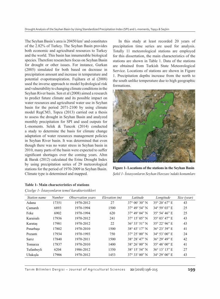
In this study at least recorded 20 years of precipitation time series are used for analysis. Totally 11 meteorological stations are employed for this dissertation, the main characteristics of the stations are shown in Table 1. Data of the stations are obtained from Turkish State Meteorological Service. Locations of stations are shown in Figure 1. Precipitation depths increase from the north to the south unlike temperature due to high geographic formations.
Figure 1- Locations of the stations in the Seyhan BasinŞekil 1- İstasyonların Seyhan Havzası’ndaki konumları
Table 1- Main characteristics of stationsÇizelge 1- İstasyonların temel karakteristikleri
Station name Number Observation years Elevation (m) Latitude Longitude Size (year)Adana 17351 1970-2012 27 37° 00’ 30” N 35° 20’ 67” E 43Çamardı 6893 1970-1994 1500 37° 49’ 54” N 34° 59’ 03” E 25Feke 6902 1970-1994 620 37° 49’ 04” N 35° 54’ 46” E 25Karaisalı 17936 1970-2012 241 37° 15’ 05” N 35° 03’ 47” E 43Karataş 17981 1970-2012 22 36° 33’ 51” N 35° 22’ 96” E 43Pınarbaşı 17802 1970-2010 1500 38° 43’ 17” N 36° 23’ 39” E 41Pozantı 17934 1970-1993 750 37° 25’ 00” N 34° 53’ 00” E 24Sarız 17840 1970-2011 1500 38° 28’ 47” N 36° 29’ 49” E 42Tomarza 17837 1970-2010 1400 38° 26’ 00” N 35° 48’ 00” E 41Tufanbeyli 6204 1986-2012 1350 38° 15’ 54” N 36° 13’ 13” E 27Ulukışla 17906 1970-2012 1453 37° 33’ 00” N 34° 29’ 00” E 43
L-momentler ve Standart Yağış İndeksi (SYİ) Yardımıyla Seyhan Havzası Kuraklık Analizi, Topçu & Seçkin
200 Ta r ı m B i l i m l e r i D e r g i s i – J o u r n a l o f A g r i c u l t u r a l S c i e n c e s 22 (2016) 196-215
2.2. Method
2.2.1. Standardized precipitation index (SPI) methodDroughts and floods are widespread subject of the hydraulic engineers and researchers. This method is used commonly to monitor the drought because of the simple algorithm and rapid response. The SPI was developed by (McKee et al 1993) for providing drought information in Colorado. Seasonal (3, 6-month time scale) or long period (9, 12, 24, 48-month time scale) drought can be analyzed, which affects all types of water resources even subsurface water. Soil moisture is affected immediately from abrupt precipitation changes. Hence, 3 or 6-month time scale monitoring is preferred. On the other hand, underground water, rivers and reservoirs do not respond rapidly to swift precipitation changes. Therefore, 12-month or long period time scale (24, 48, 72-month) monitoring is chosen. There are lots of studies about Standardized Precipitation Index for monitoring drought all around the world like (McKee et al 1993; Edwards & McKee 1997; Guttman 1999; Türkes 1999; Kömüscü 2001; Lloyd-Hughes & Saunders 2002; Tonkaz 2006; Li et al 2008; Abolverdi & Khalili 2010; Keskin & Sorman 2010). Anlı (2014) carried out a study to analysis meteorological drought in provinces of South Eastern Anatolia Region by using temporal variation of reference evapotranspiration (ET0) and RDI (Reconnaissance Drought Index). Study results show that significant increasing trends for reference evapotranspiration have been detected and according to RDI, mild drought has been experienced in general. In addition, there have been a significant amount of events where moderate and severely droughts occurred. Guenang & Kamga (2014) computed SPI using 55 years of precipitation data recorded 24 observation stations in Cameroon. Four statistical distribution functions (gamma, exponential, Weibull and lognormal) are fitted to data. Drought thresholds determined. McRoberts & Nielsen-Gammon (2012) developed high-resolution drought-monitoring tool to assess drought on multiple time scales using the SPI. Regional frequency
analysis is performed. Dutra et al (2013) assessed the predictive capabilities of an integrated drought monitoring and seasonal forecasting system (up to 5 months lead time) based on SPI. The forecasts were evaluated over four basins in Africa. Jha et al (2013) computed the SPI with monthly precipitation dataset for each of the 14 mainland agro climatic zones of India. Showed that only six out of 14 mainlands have a significant trend during summer monsoon. Blain (2012) carried out analyses by evaluating the normality assumption of the SPI distributions. Observed that Pearson III distribution was better than the Gamma 2-parameter distribution. Xie et al (2013) investigated the spatiotemporal variability of drought incidence in Pakistan during 1960-2007 by SPI for 3, 6 and 12-month scales. Analysis revealed that droughts are wide-spread and often occur over large areas. Simsek & Cakmak (2010) analyzed the drought experience in 2007-2008 Agricultural Year of Turkey. The drought was evaluated by using SPI, Percent of Normal Index (PNI) and the analyses of precipitation and temperature analysis. The SPI is the non-dimensional drought index. This index is computed for long time precipitation series for the preferred time scales. The SPI calculated by Equation 1.
5
Study results show that significant increasing trends for reference evapotranspiration have been detected and according to RDI, mild drought has been experienced in general. In addition, there have been a significant amount of events where moderate and severely droughts occurred. Guenang & Kamga (2014) computed SPI using 55 years of precipitation data recorded 24 observation stations in Cameroon. Four statistical distribution functions (gamma, exponential, Weibull and lognormal) are fitted to data. Drought thresholds determined. McRoberts & Nielsen-Gammon (2012) developed high-resolution drought-monitoring tool to assess drought on multiple time scales using the SPI. Regional frequency analysis is performed. Dutra et al (2013) assessed the predictive capabilities of an integrated drought monitoring and seasonal forecasting system (up to 5 months lead time) based on SPI. The forecasts were evaluated over four basins in Africa. Jha et al (2013) computed the SPI with monthly precipitation dataset for each of the 14 mainland agro climatic zones of India. Showed that only six out of 14 mainlands have a significant trend during summer monsoon. Blain (2012) carried out analyses by evaluating the normality assumption of the SPI distributions. Observed that Pearson III distribution was better than the Gamma 2-parameter distribution. Xie et al (2013) investigated the spatiotemporal variability of drought incidence in Pakistan during 1960-2007 by SPI for 3, 6 and 12-month scales. Analysis revealed that droughts are wide-spread and often occur over large areas. Simsek & Cakmak (2010) analyzed the drought experience in 2007-2008 Agricultural Year of Turkey. The drought was evaluated by using SPI, Percent of Normal Index (PNI) and the analyses of precipitation and temperature analysis. The SPI is the non-dimensional drought index. This index is computed for long time precipitation series for the preferred time scales. The SPI calculated by Equation 1.
SPI = (Xİ − X̅)/ σ (1) Where; SPI, standardized precipitation index; Xİ, data point; X̅ , mean; 𝜎𝜎 , standard deviation of the data
The gamma distribution is convenient for precipitation series and the distribution parameters can be
calculated by maximum likelihood approximation of Thom (1958). If precipitation data has zero values, mixed distribution by Thom (1951) can be used for incorporation of zero probability and non-zero probabilities (Equation 2).
H(x) = q + (1-q) G(x) (2)
Where; q, the probability of zero precipitation; G(x), the gamma cumulative probability function.
Probabilities calculated by Equation 2 are transformed into the standard normal distribution for calculation of the SPI values (Guttman 1998).
SPI method shows the drought category corresponds to output values (Table 2). If the SPI gives
negative values, it means there is drought and lack of precipitation; if the SPI gives positive values, it means there is no drought and enough precipitation. Yet, the negative values are getting lower, the degree of the drought shifts from no drought to extremely drought and then catastrophe bursts. And same for the positive values, if the positive values are getting higher the degree of the drought shifts from no drought to extremely wet and flash floods are seen. The drought frequency of a station is obtained by dividing drought event size by total observation size. Frequency values show us how often drought conditions happen in a station for a prespecified time scale.
(1)
Where; SPI, standardized precipitation index;
5
Study results show that significant increasing trends for reference evapotranspiration have been detected and according to RDI, mild drought has been experienced in general. In addition, there have been a significant amount of events where moderate and severely droughts occurred. Guenang & Kamga (2014) computed SPI using 55 years of precipitation data recorded 24 observation stations in Cameroon. Four statistical distribution functions (gamma, exponential, Weibull and lognormal) are fitted to data. Drought thresholds determined. McRoberts & Nielsen-Gammon (2012) developed high-resolution drought-monitoring tool to assess drought on multiple time scales using the SPI. Regional frequency analysis is performed. Dutra et al (2013) assessed the predictive capabilities of an integrated drought monitoring and seasonal forecasting system (up to 5 months lead time) based on SPI. The forecasts were evaluated over four basins in Africa. Jha et al (2013) computed the SPI with monthly precipitation dataset for each of the 14 mainland agro climatic zones of India. Showed that only six out of 14 mainlands have a significant trend during summer monsoon. Blain (2012) carried out analyses by evaluating the normality assumption of the SPI distributions. Observed that Pearson III distribution was better than the Gamma 2-parameter distribution. Xie et al (2013) investigated the spatiotemporal variability of drought incidence in Pakistan during 1960-2007 by SPI for 3, 6 and 12-month scales. Analysis revealed that droughts are wide-spread and often occur over large areas. Simsek & Cakmak (2010) analyzed the drought experience in 2007-2008 Agricultural Year of Turkey. The drought was evaluated by using SPI, Percent of Normal Index (PNI) and the analyses of precipitation and temperature analysis. The SPI is the non-dimensional drought index. This index is computed for long time precipitation series for the preferred time scales. The SPI calculated by Equation 1.
SPI = (Xİ − X̅)/ σ (1) Where; SPI, standardized precipitation index; Xİ, data point; X̅ , mean; 𝜎𝜎 , standard deviation of the data
The gamma distribution is convenient for precipitation series and the distribution parameters can be
calculated by maximum likelihood approximation of Thom (1958). If precipitation data has zero values, mixed distribution by Thom (1951) can be used for incorporation of zero probability and non-zero probabilities (Equation 2).
H(x) = q + (1-q) G(x) (2)
Where; q, the probability of zero precipitation; G(x), the gamma cumulative probability function.
Probabilities calculated by Equation 2 are transformed into the standard normal distribution for calculation of the SPI values (Guttman 1998).
SPI method shows the drought category corresponds to output values (Table 2). If the SPI gives
negative values, it means there is drought and lack of precipitation; if the SPI gives positive values, it means there is no drought and enough precipitation. Yet, the negative values are getting lower, the degree of the drought shifts from no drought to extremely drought and then catastrophe bursts. And same for the positive values, if the positive values are getting higher the degree of the drought shifts from no drought to extremely wet and flash floods are seen. The drought frequency of a station is obtained by dividing drought event size by total observation size. Frequency values show us how often drought conditions happen in a station for a prespecified time scale.
, data point;
5
Study results show that significant increasing trends for reference evapotranspiration have been detected and according to RDI, mild drought has been experienced in general. In addition, there have been a significant amount of events where moderate and severely droughts occurred. Guenang & Kamga (2014) computed SPI using 55 years of precipitation data recorded 24 observation stations in Cameroon. Four statistical distribution functions (gamma, exponential, Weibull and lognormal) are fitted to data. Drought thresholds determined. McRoberts & Nielsen-Gammon (2012) developed high-resolution drought-monitoring tool to assess drought on multiple time scales using the SPI. Regional frequency analysis is performed. Dutra et al (2013) assessed the predictive capabilities of an integrated drought monitoring and seasonal forecasting system (up to 5 months lead time) based on SPI. The forecasts were evaluated over four basins in Africa. Jha et al (2013) computed the SPI with monthly precipitation dataset for each of the 14 mainland agro climatic zones of India. Showed that only six out of 14 mainlands have a significant trend during summer monsoon. Blain (2012) carried out analyses by evaluating the normality assumption of the SPI distributions. Observed that Pearson III distribution was better than the Gamma 2-parameter distribution. Xie et al (2013) investigated the spatiotemporal variability of drought incidence in Pakistan during 1960-2007 by SPI for 3, 6 and 12-month scales. Analysis revealed that droughts are wide-spread and often occur over large areas. Simsek & Cakmak (2010) analyzed the drought experience in 2007-2008 Agricultural Year of Turkey. The drought was evaluated by using SPI, Percent of Normal Index (PNI) and the analyses of precipitation and temperature analysis. The SPI is the non-dimensional drought index. This index is computed for long time precipitation series for the preferred time scales. The SPI calculated by Equation 1.
SPI = (Xİ − X̅)/ σ (1) Where; SPI, standardized precipitation index; Xİ, data point; X̅ , mean; 𝜎𝜎 , standard deviation of the data
The gamma distribution is convenient for precipitation series and the distribution parameters can be
calculated by maximum likelihood approximation of Thom (1958). If precipitation data has zero values, mixed distribution by Thom (1951) can be used for incorporation of zero probability and non-zero probabilities (Equation 2).
H(x) = q + (1-q) G(x) (2)
Where; q, the probability of zero precipitation; G(x), the gamma cumulative probability function.
Probabilities calculated by Equation 2 are transformed into the standard normal distribution for calculation of the SPI values (Guttman 1998).
SPI method shows the drought category corresponds to output values (Table 2). If the SPI gives
negative values, it means there is drought and lack of precipitation; if the SPI gives positive values, it means there is no drought and enough precipitation. Yet, the negative values are getting lower, the degree of the drought shifts from no drought to extremely drought and then catastrophe bursts. And same for the positive values, if the positive values are getting higher the degree of the drought shifts from no drought to extremely wet and flash floods are seen. The drought frequency of a station is obtained by dividing drought event size by total observation size. Frequency values show us how often drought conditions happen in a station for a prespecified time scale.
, mean;
5
Study results show that significant increasing trends for reference evapotranspiration have been detected and according to RDI, mild drought has been experienced in general. In addition, there have been a significant amount of events where moderate and severely droughts occurred. Guenang & Kamga (2014) computed SPI using 55 years of precipitation data recorded 24 observation stations in Cameroon. Four statistical distribution functions (gamma, exponential, Weibull and lognormal) are fitted to data. Drought thresholds determined. McRoberts & Nielsen-Gammon (2012) developed high-resolution drought-monitoring tool to assess drought on multiple time scales using the SPI. Regional frequency analysis is performed. Dutra et al (2013) assessed the predictive capabilities of an integrated drought monitoring and seasonal forecasting system (up to 5 months lead time) based on SPI. The forecasts were evaluated over four basins in Africa. Jha et al (2013) computed the SPI with monthly precipitation dataset for each of the 14 mainland agro climatic zones of India. Showed that only six out of 14 mainlands have a significant trend during summer monsoon. Blain (2012) carried out analyses by evaluating the normality assumption of the SPI distributions. Observed that Pearson III distribution was better than the Gamma 2-parameter distribution. Xie et al (2013) investigated the spatiotemporal variability of drought incidence in Pakistan during 1960-2007 by SPI for 3, 6 and 12-month scales. Analysis revealed that droughts are wide-spread and often occur over large areas. Simsek & Cakmak (2010) analyzed the drought experience in 2007-2008 Agricultural Year of Turkey. The drought was evaluated by using SPI, Percent of Normal Index (PNI) and the analyses of precipitation and temperature analysis. The SPI is the non-dimensional drought index. This index is computed for long time precipitation series for the preferred time scales. The SPI calculated by Equation 1.
SPI = (Xİ − X̅)/ σ (1) Where; SPI, standardized precipitation index; Xİ, data point; X̅ , mean; 𝜎𝜎 , standard deviation of the data
The gamma distribution is convenient for precipitation series and the distribution parameters can be
calculated by maximum likelihood approximation of Thom (1958). If precipitation data has zero values, mixed distribution by Thom (1951) can be used for incorporation of zero probability and non-zero probabilities (Equation 2).
H(x) = q + (1-q) G(x) (2)
Where; q, the probability of zero precipitation; G(x), the gamma cumulative probability function.
Probabilities calculated by Equation 2 are transformed into the standard normal distribution for calculation of the SPI values (Guttman 1998).
SPI method shows the drought category corresponds to output values (Table 2). If the SPI gives
negative values, it means there is drought and lack of precipitation; if the SPI gives positive values, it means there is no drought and enough precipitation. Yet, the negative values are getting lower, the degree of the drought shifts from no drought to extremely drought and then catastrophe bursts. And same for the positive values, if the positive values are getting higher the degree of the drought shifts from no drought to extremely wet and flash floods are seen. The drought frequency of a station is obtained by dividing drought event size by total observation size. Frequency values show us how often drought conditions happen in a station for a prespecified time scale.
, standard deviation of the data
The gamma distribution is convenient for precipitation series and the distribution parameters can be calculated by maximum likelihood approximation of Thom (1958). If precipitation data has zero values, mixed distribution by Thom (1951) can be used for incorporation of zero probability and non-zero probabilities (Equation 2).
5
Study results show that significant increasing trends for reference evapotranspiration have been detected and according to RDI, mild drought has been experienced in general. In addition, there have been a significant amount of events where moderate and severely droughts occurred. Guenang & Kamga (2014) computed SPI using 55 years of precipitation data recorded 24 observation stations in Cameroon. Four statistical distribution functions (gamma, exponential, Weibull and lognormal) are fitted to data. Drought thresholds determined. McRoberts & Nielsen-Gammon (2012) developed high-resolution drought-monitoring tool to assess drought on multiple time scales using the SPI. Regional frequency analysis is performed. Dutra et al (2013) assessed the predictive capabilities of an integrated drought monitoring and seasonal forecasting system (up to 5 months lead time) based on SPI. The forecasts were evaluated over four basins in Africa. Jha et al (2013) computed the SPI with monthly precipitation dataset for each of the 14 mainland agro climatic zones of India. Showed that only six out of 14 mainlands have a significant trend during summer monsoon. Blain (2012) carried out analyses by evaluating the normality assumption of the SPI distributions. Observed that Pearson III distribution was better than the Gamma 2-parameter distribution. Xie et al (2013) investigated the spatiotemporal variability of drought incidence in Pakistan during 1960-2007 by SPI for 3, 6 and 12-month scales. Analysis revealed that droughts are wide-spread and often occur over large areas. Simsek & Cakmak (2010) analyzed the drought experience in 2007-2008 Agricultural Year of Turkey. The drought was evaluated by using SPI, Percent of Normal Index (PNI) and the analyses of precipitation and temperature analysis. The SPI is the non-dimensional drought index. This index is computed for long time precipitation series for the preferred time scales. The SPI calculated by Equation 1.
SPI = (Xİ − X̅)/ σ (1) Where; SPI, standardized precipitation index; Xİ, data point; X̅ , mean; 𝜎𝜎 , standard deviation of the data
The gamma distribution is convenient for precipitation series and the distribution parameters can be
calculated by maximum likelihood approximation of Thom (1958). If precipitation data has zero values, mixed distribution by Thom (1951) can be used for incorporation of zero probability and non-zero probabilities (Equation 2).
H(x) = q + (1-q) G(x) (2)
Where; q, the probability of zero precipitation; G(x), the gamma cumulative probability function.
Probabilities calculated by Equation 2 are transformed into the standard normal distribution for calculation of the SPI values (Guttman 1998).
SPI method shows the drought category corresponds to output values (Table 2). If the SPI gives
negative values, it means there is drought and lack of precipitation; if the SPI gives positive values, it means there is no drought and enough precipitation. Yet, the negative values are getting lower, the degree of the drought shifts from no drought to extremely drought and then catastrophe bursts. And same for the positive values, if the positive values are getting higher the degree of the drought shifts from no drought to extremely wet and flash floods are seen. The drought frequency of a station is obtained by dividing drought event size by total observation size. Frequency values show us how often drought conditions happen in a station for a prespecified time scale.
(2)
Where; q, the probability of zero precipitation; G(x), the gamma cumulative probability function. Probabilities calculated by Equation 2 are transformed into the standard normal distribution for calculation of the SPI values (Guttman 1998).

Drought Analysis of the Seyhan Basin by Using Standardized Precipitation Index (SPI) and L-moments, Topçu & Seçkin
201Ta r ı m B i l i m l e r i D e r g i s i – J o u r n a l o f A g r i c u l t u r a l S c i e n c e s 22 (2016) 196-215
SPI method shows the drought category corresponds to output values (Table 2). If the SPI gives negative values, it means there is drought and lack of precipitation; if the SPI gives positive values, it means there is no drought and enough precipitation. Yet, the negative values are getting lower, the degree of the drought shifts from no drought to extremely drought and then catastrophe bursts. And same for the positive values, if the positive values are getting higher the degree of the drought shifts from no drought to extremely wet and flash floods are seen. The drought frequency of a station is obtained by dividing drought event size by total observation size. Frequency values show us how often drought conditions happen in a station for a prespecified time scale.
Table 2- Standardized precipitation index categoriesÇizelge 2- Standart yağış indeksi kategorileri
SPI index values Drought category
2.00 or more Extreme Wet
1.50 - 1.99 Severe Wet
1.00 - 1.49 Moderate Wet
0.0 - 0.99 Mild Wet
0.0 - (-0.99) Mild Drought
(-1.00) - (-1.49) Moderate Drought
(-1.50) - (-1.99) Severe Drought
(-2.00) or less Extreme Drought
2.2.2. Index-flood methodIndex flood method is a reliable procedure as to pooling summary statistics from different data samples. Its early applications were based on flood data in hydrology (Dalrymple 1960). However, Hosking & Wallis (1997) pointed out that this method can be applicable to every kind of data.
According to the index-flood method, the exceedance probability distribution of annual peak discharge is accepted as identical for hydrologically homogeneous regions except for a site-specific scaling factor called the index flood (Dalrymple 1960; Hosking & Wallis 1997).
The important physiographic and meteorological characteristics of a basin are reflected by this index flood parameter. In this method, the relationship in Equation 3 is recommended to estimate the flood quantile QT.
6
Table 2- Standardized precipitation index categories Çizelge 2- Standart yağış indeksi kategorileri SPI index values Drought category
2.00 or more Extreme Wet 1.50 - 1.99 Severe Wet
1.00 - 1.49 Moderate Wet
0.0 - 0.99 Mild Wet
0.0 - (-0.99) Mild Drought
(-1.00) - (-1.49) Moderate Drought
(-1.50) - (-1.99) Severe Drought
(-2.00) or less Extreme Drought
2.2.2. Index-flood method Index flood method is a reliable procedure as to pooling summary statistics from different data samples. Its early applications were based on flood data in hydrology (Dalrymple 1960). However, Hosking & Wallis (1997) pointed out that this method can be applicable to every kind of data.
According to the index-flood method, the exceedance probability distribution of annual peak discharge is accepted as identical for hydrologically homogeneous regions except for a site-specific scaling factor called the index flood (Dalrymple 1960; Hosking & Wallis 1997).
The important physiographic and meteorological characteristics of a basin are reflected by this index
flood parameter. In this method, the relationship in Equation 3 is recommended to estimate the flood quantile QT.
QT = qTμi (3)
Where; T, return period at site i; μ, the product of index flood (average likely flood); q, the regional
growth factor. μ is also the function basin area and slope. q is a dimensionless frequency distribution quantity common to all sites within a hydrologic homogeneous region.
A relationship based on available information gathered from the gauged sites is recommended to estimate index flood.
Once an appropriate frequency distribution has been found within a hydrologic region with N sites,
regional growth curves are determined to represent the relationship between qT and T. It can be summarized that index flood method based on regional flood-frequency analysis has three
steps: hydrologic homogeneous regionalization, selection of regional frequency distribution and estimation of index flood relationship. To estimate design flood of any intermediate values of return periods (e.g. T= 2, 5, 10, 20, 50, 100 …years), the index flood-based regional relationships can be used.
2.2.3. L-moments method L-moments method was developed by (Hosking 1986; 1990). This method is widely used for regionalization, estimation parameters and determine the quantiles. L-moments method is the linear function of the probability weighted moments (PWM). There are really comprehensive studies in literature like Dalrymple (1960), Landwehr et al (1979a; 1979b; 1979c), Hosking (1986; 1990), Gebeyehu (1989), Hosking & Wallis (1993;1997), Fowler & Kilsbyc (2003), Eslamian & Feizi (2006), Seckin & Yurtal (2007; 2008), Norbiato et al (2007), Parida & Moalafhi (2008), Seckin et al (2010a; 2010b; 2011), Dodangeh et al (2011) and Tallaksen et al (2011). Anlı et al (2009) conducted a study to determine regional analysis of the annual maxima precipitation influenced on floods in Trabzon Province. Annual maxima precipitation series of 10-78 years of 10 precipitation gauging stations over Trabzon
(3)Where; T, return period at site i; μ, the product
of index flood (average likely flood); q, the regional growth factor. μ is also the function basin area and slope. q is a dimensionless frequency distribution quantity common to all sites within a hydrologic homogeneous region.
A relationship based on available information gathered from the gauged sites is recommended to estimate index flood.
Once an appropriate frequency distribution has been found within a hydrologic region with N sites, regional growth curves are determined to represent the relationship between qT and T.
It can be summarized that index flood method based on regional flood-frequency analysis has three steps: hydrologic homogeneous regionalization, selection of regional frequency distribution and estimation of index flood relationship. To estimate design flood of any intermediate values of return periods (e.g. T= 2, 5, 10, 20, 50, 100 …years), the index flood-based regional relationships can be used.
2.2.3. L-moments methodL-moments method was developed by (Hosking 1986; 1990). This method is widely used for regionalization, estimation parameters and determine the quantiles. L-moments method is the linear function of the probability weighted moments (PWM). There are really comprehensive studies in literature like Dalrymple (1960), Landwehr et al (1979a; 1979b; 1979c), Hosking (1986; 1990), Gebeyehu (1989), Hosking & Wallis (1993;1997), Fowler & Kilsbyc (2003), Eslamian & Feizi (2006), Seckin & Yurtal (2008), Norbiato et al (2007), Parida & Moalafhi (2008), Seckin et al (2010a; 2010b; 2011), Dodangeh et al (2011) and Tallaksen et al (2011). Anlı et al (2009) conducted a study to
L-momentler ve Standart Yağış İndeksi (SYİ) Yardımıyla Seyhan Havzası Kuraklık Analizi, Topçu & Seçkin
202 Ta r ı m B i l i m l e r i D e r g i s i – J o u r n a l o f A g r i c u l t u r a l S c i e n c e s 22 (2016) 196-215
determine regional analysis of the annual maxima precipitation influenced on floods in Trabzon Province. Annual maxima precipitation series of 10-78 years of 10 precipitation gauging stations over Trabzon Province were used as a material. Probability parameter estimation and regional analysis were used based on L-moments statistics. Some quantile functions were obtained through Monte Carlo simulation techniques. For flood management and the design of urban drainage networks, useful precipitation values were estimated for some quantile probabilities of the at-site and regional analysis for the Generalized Logistics and Generalized Extreme Value distributions obtained from simulation. Shi et al (2010) screened the data from 12 stream flow gauging sites of the Wujiang water system in Guizhou Province by using the discordancy measure, and homogeneity of the region is then tested employing the L-moments-based heterogeneity measure. Eslamian et al (2012) used two indexes of cumulative precipitation deficit (CPD) and maximum precipitation deficit (MPD) for evaluating the severity of drought in a certain month and regional frequency analysis has been carried out by L-moments. Gingras & Adamowski (1994) conduct a simulation study to compare parametric L-moments and nonparametric approaches in flood frequency analysis. Saf (2009) carried out a study to determine regional probability distributions for the annual maximum flood data observed at 45 streamflow gauging sites in the Kucuk and Buyuk Menderes River Basins in Turkey using index flood L moments. The generalized normal extreme value distribution has been identified as the best-fit distribution for the upper- and lower-Menderes subregions. Aydogan et al (2014) performed a regional flood frequency analysis of Çoruh Basin with the L-moments method. The flow values determined from the quantiles estimated with the L-moments method were compared with those estimated previously with an at-site frequency analysis (Gumbel distribution) on the basin master plan for four large dams in the Çoruh Basin. Dubey (2014) used the L-Moments for parameter estimation of Generalized Extreme Value (GEV) distribution. Regional flood frequency relationship
for the chosen basin is developed utilizing GEV distribution.
L-moments are defined in Equation 4 (Hosking & Wallis 1997).
7
Province were used as a material. Probability parameter estimation and regional analysis were used based on L-moments statistics. Some quantile functions were obtained through Monte Carlo simulation techniques. For flood management and the design of urban drainage networks, useful precipitation values were estimated for some quantile probabilities of the at-site and regional analysis for the Generalized Logistics and Generalized Extreme Value distributions obtained from simulation. Shi et al (2010) screened the data from 12 stream flow gauging sites of the Wujiang water system in Guizhou Province by using the discordancy measure, and homogeneity of the region is then tested employing the L-moments-based heterogeneity measure. Eslamian et al (2012) used two indexes of cumulative precipitation deficit (CPD) and maximum precipitation deficit (MPD) for evaluating the severity of drought in a certain month and regional frequency analysis has been carried out by L-moments. Gingras & Adamowski (1994) conduct a simulation study to compare parametric L-moments and nonparametric approaches in flood frequency analysis. Saf (2009) carried out a study to determine regional probability distributions for the annual maximum flood data observed at 45 streamflow gauging sites in the Kucuk and Buyuk Menderes River Basins in Turkey using index flood L moments. The generalized normal extreme value distribution has been identified as the best-fit distribution for the upper- and lower-Menderes subregions. Aydogan et al (2014) performed a regional flood frequency analysis of Çoruh Basin with the L-moments method. The flow values determined from the quantiles estimated with the L-moments method were compared with those estimated previously with an at-site frequency analysis (Gumbel distribution) on the basin master plan for four large dams in the Çoruh Basin. Dubey (2014) used the L-Moments for parameter estimation of Generalized Extreme Value (GEV) distribution. Regional flood frequency relationship for the chosen basin is developed utilizing GEV distribution. L-moments are defined in Equation 4 (Hosking & Wallis 1997).
1001 M
1001102 MM2 (4)
1001101203 MM6M6
1001101201304 MM12M30M20
The significance or meaning of this would be that: M100 is the zeroth, M110 is the first, M120 is the second, and M130 is the third probability weighted moments. Followed by these definitions listed below.
- The L-mean, 1, is a measure of central tendency which is the same as the conventional mean. -The L-standard deviation, 2, is a measure of dispersion, as 3 and 4 are the third and the fourth L-moments. -M110 is the expected value of the random variable, x, weighted by its probability of non-exceedance, Pnex. -M120 and M130 are the expected values of x weighted by (Pnex)2 and (Pnex)3, respectively. -The dimensionless L-moment ratios are defined by Hosking (1990) as in Equation 5.
2= 2/ 1 (L-variation coefficient, L-Cv) 3= 3/ 2 (L-skewness coefficient, L-Cs) (5) 4= 4/ 2 (L-kurtosis coefficient, L-Ck)
Stedinger et al (1993) developed the relationships for the parameters and the L-moments for various
distributions. For a Probability Distribution that takes on merely positive values, τ2 varies within the interval: 0 τ2
< 1, and the other ratios are within: –1 < τ3 < +1, and –1 < τ4 < +1. These properties would be claimed to be an advantage over the Conventional Coefficients of the skew and the kurtosis, because as the latter mentioned may assume very high magnitudes and former would constantly remain in the reasonable and confined interval of (-1, +1).
The arithmetical average of a sample series is the estimate of 1. The estimates of the L-coefficients of
τ2, τ3, and τ4, are calculated using the recorded sample series with the aid of a suitable plotting position
(4)
The significance or meaning of this would be that: M100 is the zeroth, M110 is the first, M120 is the second, and M130 is the third probability weighted moments. Followed by these definitions listed below.- The L-mean, λ1, is a measure of central tendency
which is the same as the conventional mean.- The L-standard deviation, λ2, is a measure of
dispersion, as λ3 and λ4 are the third and the fourth L-moments.
- M110 is the expected value of the random variable, x, weighted by its probability of non-exceedance, Pnex.
- M120 and M130 are the expected values of x weighted by (Pnex)
2 and (Pnex)3, respectively.
- The dimensionless L-moment ratios are defined by Hosking (1990) as in Equation 5.
7
Province were used as a material. Probability parameter estimation and regional analysis were used based on L-moments statistics. Some quantile functions were obtained through Monte Carlo simulation techniques. For flood management and the design of urban drainage networks, useful precipitation values were estimated for some quantile probabilities of the at-site and regional analysis for the Generalized Logistics and Generalized Extreme Value distributions obtained from simulation. Shi et al (2010) screened the data from 12 stream flow gauging sites of the Wujiang water system in Guizhou Province by using the discordancy measure, and homogeneity of the region is then tested employing the L-moments-based heterogeneity measure. Eslamian et al (2012) used two indexes of cumulative precipitation deficit (CPD) and maximum precipitation deficit (MPD) for evaluating the severity of drought in a certain month and regional frequency analysis has been carried out by L-moments. Gingras & Adamowski (1994) conduct a simulation study to compare parametric L-moments and nonparametric approaches in flood frequency analysis. Saf (2009) carried out a study to determine regional probability distributions for the annual maximum flood data observed at 45 streamflow gauging sites in the Kucuk and Buyuk Menderes River Basins in Turkey using index flood L moments. The generalized normal extreme value distribution has been identified as the best-fit distribution for the upper- and lower-Menderes subregions. Aydogan et al (2014) performed a regional flood frequency analysis of Çoruh Basin with the L-moments method. The flow values determined from the quantiles estimated with the L-moments method were compared with those estimated previously with an at-site frequency analysis (Gumbel distribution) on the basin master plan for four large dams in the Çoruh Basin. Dubey (2014) used the L-Moments for parameter estimation of Generalized Extreme Value (GEV) distribution. Regional flood frequency relationship for the chosen basin is developed utilizing GEV distribution. L-moments are defined in Equation 4 (Hosking & Wallis 1997).
1001 M
1001102 MM2 (4)
1001101203 MM6M6
1001101201304 MM12M30M20
The significance or meaning of this would be that: M100 is the zeroth, M110 is the first, M120 is the second, and M130 is the third probability weighted moments. Followed by these definitions listed below.
- The L-mean, 1, is a measure of central tendency which is the same as the conventional mean. -The L-standard deviation, 2, is a measure of dispersion, as 3 and 4 are the third and the fourth L-moments. -M110 is the expected value of the random variable, x, weighted by its probability of non-exceedance, Pnex. -M120 and M130 are the expected values of x weighted by (Pnex)2 and (Pnex)3, respectively. -The dimensionless L-moment ratios are defined by Hosking (1990) as in Equation 5.
2= 2/ 1 (L-variation coefficient, L-Cv) 3= 3/ 2 (L-skewness coefficient, L-Cs) (5) 4= 4/ 2 (L-kurtosis coefficient, L-Ck)
Stedinger et al (1993) developed the relationships for the parameters and the L-moments for various
distributions. For a Probability Distribution that takes on merely positive values, τ2 varies within the interval: 0 τ2
< 1, and the other ratios are within: –1 < τ3 < +1, and –1 < τ4 < +1. These properties would be claimed to be an advantage over the Conventional Coefficients of the skew and the kurtosis, because as the latter mentioned may assume very high magnitudes and former would constantly remain in the reasonable and confined interval of (-1, +1).
The arithmetical average of a sample series is the estimate of 1. The estimates of the L-coefficients of
τ2, τ3, and τ4, are calculated using the recorded sample series with the aid of a suitable plotting position
(5)
Stedinger et al (1993) developed the relationships for the parameters and the L-moments for various distributions.
For a Probability Distribution that takes on merely positive values, τ2 varies within the interval: 0 ≤ τ2 < 1, and the other ratios are within: –1 < τ3 < +1, and –1 < τ4 < +1. These properties would be claimed to be an advantage over the Conventional Coefficients of the skew and the kurtosis, because as the latter mentioned may assume very high magnitudes and former would constantly remain in the reasonable and confined interval of (-1, +1).
Drought Analysis of the Seyhan Basin by Using Standardized Precipitation Index (SPI) and L-moments, Topçu & Seçkin
203Ta r ı m B i l i m l e r i D e r g i s i – J o u r n a l o f A g r i c u l t u r a l S c i e n c e s 22 (2016) 196-215
The arithmetical average of a sample series is the estimate of λ1. The estimates of the L-coefficients of τ2, τ3, and τ4, are calculated using the recorded sample series with the aid of a suitable plotting position formula. For which the biased-Landwehr formula is preferred, as done in this study also, to estimate Pnex’s of the elements of the series.
2.2.4. Homogeneity testsHosking (1991; 1993) recommended the following three statistical measures for homogeneity tests as discordancy measure (Di), heterogeneity measure (H) and goodness of fit measure (Z).
2.2.5. Discordancy measure (Di)This test is based on the L-moments ratios and utilized to identify the sites of a given group that are discordant with the other sites of entire group. Discordancy measure depends on the number of sites. Discordant sites should be discarded from the analyzed or evaluated in another region. Hosking & Wallis (1997) presented a table which shows critical values of discordancy statistic correspond to a number of sites (Table 3). The site is accepted to be harmonious if discordancy value of site is smaller than the critical value of the discordancy statistic.
Table 3- Critical values of discordancy statistic, Di
Çizelge 3- Uyumsuzluk ölçüsünün kritik değerleri, Di
No. of sites in region
Critical value
No. of sites in region
Critical value
5 1.333 11 2.6326 1.648 12 2.7577 1.917 13 2.8698 2.14 14 2.9719 2.329 ≥15 310 2.491
Discordancy measure (Di) is defined in Equation 6, 7 and 8.
( ) ( )uuSuu31D i
1Tii −−= − (6)
8
formula. For which the biased-Landwehr formula is preferred, as done in this study also, to estimate Pnex’s of the elements of the series.
2.2.4. Homogeneity tests Hosking (1991; 1993) recommended the following three statistical measures for homogeneity tests as discordancy measure (Di), heterogeneity measure (H) and goodness of fit measure (Z). 2.2.5. Discordancy measure (Di) This test is based on the L-moments ratios and utilized to identify the sites of a given group that are discordant with the other sites of entire group. Discordancy measure depends on the number of sites. Discordant sites should be discarded from the analyzed or evaluated in another region. Hosking & Wallis (1997) presented a table which shows critical values of discordancy statistic correspond to a number of sites (Table 3). The site is accepted to be harmonious if discordancy value of site is smaller than the critical value of the discordancy statistic. Table 3- Critical values of discordancy statistic, Di
Çizelge 3- Uyumsuzluk ölçüsünün kritik değerleri, Di No. of sites in region
Critical value
No. of sites in region
Critical value
5 1.333 11 2.632 6 1.648 12 2.757 7 1.917 13 2.869 8 2.14 14 2.971 9 2.329 ≥15 3
10 2.491 Discordancy measure (Di) is defined in Equation 6, 7 and 8.
uuSuu31D i
1Tii (6)
u̅ = N−1 ∑ uiNi=1 (7)
S = ∑ (ui − u̅)(ui − u̅)TN
i=1 (8)
Where; ui, vector of LCv, LCs, LCk for a site I; S, covariance matrix of ui; u , mean of vector ui
2.2.6. Heterogeneity measure (H) The heterogeneity measure (Hi) is proposed for identification of the degree of heterogeneity of group of sites and Hi can be estimated by Equation 9 and 10.
v
vVH (9)
)4,3,2s(nτnτN
1ii
N
1i
isi
Rs (10)
Where; V, weighted standard deviation of L-coefficient of variation values; and , the mean and
standard deviation of a number of simulations of V.
(7)
8
formula. For which the biased-Landwehr formula is preferred, as done in this study also, to estimate Pnex’s of the elements of the series.
2.2.4. Homogeneity tests Hosking (1991; 1993) recommended the following three statistical measures for homogeneity tests as discordancy measure (Di), heterogeneity measure (H) and goodness of fit measure (Z). 2.2.5. Discordancy measure (Di) This test is based on the L-moments ratios and utilized to identify the sites of a given group that are discordant with the other sites of entire group. Discordancy measure depends on the number of sites. Discordant sites should be discarded from the analyzed or evaluated in another region. Hosking & Wallis (1997) presented a table which shows critical values of discordancy statistic correspond to a number of sites (Table 3). The site is accepted to be harmonious if discordancy value of site is smaller than the critical value of the discordancy statistic. Table 3- Critical values of discordancy statistic, Di
Çizelge 3- Uyumsuzluk ölçüsünün kritik değerleri, Di No. of sites in region
Critical value
No. of sites in region
Critical value
5 1.333 11 2.632 6 1.648 12 2.757 7 1.917 13 2.869 8 2.14 14 2.971 9 2.329 ≥15 3
10 2.491 Discordancy measure (Di) is defined in Equation 6, 7 and 8.
uuSuu31D i
1Tii (6)
u̅ = N−1 ∑ uiNi=1 (7)
S = ∑ (ui − u̅)(ui − u̅)TN
i=1 (8)
Where; ui, vector of LCv, LCs, LCk for a site I; S, covariance matrix of ui; u , mean of vector ui
2.2.6. Heterogeneity measure (H) The heterogeneity measure (Hi) is proposed for identification of the degree of heterogeneity of group of sites and Hi can be estimated by Equation 9 and 10.
v
vVH (9)
)4,3,2s(nτnτN
1ii
N
1i
isi
Rs (10)
Where; V, weighted standard deviation of L-coefficient of variation values; and , the mean and
standard deviation of a number of simulations of V.
(8)
Where; ui, vector of LCv, LCs, LCk for a site I; S, covariance matrix of ui; u , mean of vector ui
2.2.6. Heterogeneity measure (H)The heterogeneity measure (Hi) is proposed for identification of the degree of heterogeneity of group of sites and Hi can be estimated by Equation 9 and 10.
8
formula. For which the biased-Landwehr formula is preferred, as done in this study also, to estimate Pnex’s of the elements of the series.
2.2.4. Homogeneity tests Hosking (1991; 1993) recommended the following three statistical measures for homogeneity tests as discordancy measure (Di), heterogeneity measure (H) and goodness of fit measure (Z). 2.2.5. Discordancy measure (Di) This test is based on the L-moments ratios and utilized to identify the sites of a given group that are discordant with the other sites of entire group. Discordancy measure depends on the number of sites. Discordant sites should be discarded from the analyzed or evaluated in another region. Hosking & Wallis (1997) presented a table which shows critical values of discordancy statistic correspond to a number of sites (Table 3). The site is accepted to be harmonious if discordancy value of site is smaller than the critical value of the discordancy statistic. Table 3- Critical values of discordancy statistic, Di
Çizelge 3- Uyumsuzluk ölçüsünün kritik değerleri, Di No. of sites in region
Critical value
No. of sites in region
Critical value
5 1.333 11 2.632 6 1.648 12 2.757 7 1.917 13 2.869 8 2.14 14 2.971 9 2.329 ≥15 3
10 2.491 Discordancy measure (Di) is defined in Equation 6, 7 and 8.
uuSuu31D i
1Tii (6)
u̅ = N−1 ∑ uiNi=1 (7)
S = ∑ (ui − u̅)(ui − u̅)TN
i=1 (8)
Where; ui, vector of LCv, LCs, LCk for a site I; S, covariance matrix of ui; u , mean of vector ui
2.2.6. Heterogeneity measure (H) The heterogeneity measure (Hi) is proposed for identification of the degree of heterogeneity of group of sites and Hi can be estimated by Equation 9 and 10.
v
vVH (9)
)4,3,2s(nτnτN
1ii
N
1i
isi
Rs (10)
Where; V, weighted standard deviation of L-coefficient of variation values; and , the mean and
standard deviation of a number of simulations of V.
(9)
8
formula. For which the biased-Landwehr formula is preferred, as done in this study also, to estimate Pnex’s of the elements of the series.
2.2.4. Homogeneity tests Hosking (1991; 1993) recommended the following three statistical measures for homogeneity tests as discordancy measure (Di), heterogeneity measure (H) and goodness of fit measure (Z). 2.2.5. Discordancy measure (Di) This test is based on the L-moments ratios and utilized to identify the sites of a given group that are discordant with the other sites of entire group. Discordancy measure depends on the number of sites. Discordant sites should be discarded from the analyzed or evaluated in another region. Hosking & Wallis (1997) presented a table which shows critical values of discordancy statistic correspond to a number of sites (Table 3). The site is accepted to be harmonious if discordancy value of site is smaller than the critical value of the discordancy statistic. Table 3- Critical values of discordancy statistic, Di
Çizelge 3- Uyumsuzluk ölçüsünün kritik değerleri, Di No. of sites in region
Critical value
No. of sites in region
Critical value
5 1.333 11 2.632 6 1.648 12 2.757 7 1.917 13 2.869 8 2.14 14 2.971 9 2.329 ≥15 3
10 2.491 Discordancy measure (Di) is defined in Equation 6, 7 and 8.
uuSuu31D i
1Tii (6)
u̅ = N−1 ∑ uiNi=1 (7)
S = ∑ (ui − u̅)(ui − u̅)TN
i=1 (8)
Where; ui, vector of LCv, LCs, LCk for a site I; S, covariance matrix of ui; u , mean of vector ui
2.2.6. Heterogeneity measure (H) The heterogeneity measure (Hi) is proposed for identification of the degree of heterogeneity of group of sites and Hi can be estimated by Equation 9 and 10.
v
vVH (9)
)4,3,2s(nτnτN
1ii
N
1i
isi
Rs (10)
Where; V, weighted standard deviation of L-coefficient of variation values; and , the mean and
standard deviation of a number of simulations of V.
( ) )4,3,2s(nônôN
1ii
N
1i
isi
Rs =∑∑=
== (10)
Where; V, weighted standard deviation of L-coefficient of variation values; µυ and συ, the mean and standard deviation of a number of simulations of V.
Suppose that the proposed region has N sites, with site i having record length ni and sample L-moment ratios τ2
(i), τ3(i), τ4
(i). Denote by τ2(R), τ3
(R), τ4
(R) the regional average L-Cv, L-Skewness and L-Kurtosis. V1, weighted standard deviation of L-coefficient of variation values can be expressed as Equation 11.
(11)
It is possible to construct heterogeneity measures in which V in equation (11) is replaced by other measures of between-site dispersion of sample L-moments. One of the measures is based on L-Cv and L-Skewness (V2) can be expressed as Equation 12.
(12)
and the other based on L-Skewness and L-Kurtosis (V3) can be expressed as Equation 13.
(13)
If heterogeneity of a region H<1 then the region is acceptably homogeneous. 1≤H<2, then the region

L-momentler ve Standart Yağış İndeksi (SYİ) Yardımıyla Seyhan Havzası Kuraklık Analizi, Topçu & Seçkin
204 Ta r ı m B i l i m l e r i D e r g i s i – J o u r n a l o f A g r i c u l t u r a l S c i e n c e s 22 (2016) 196-215
is possibly heterogeneous. H≥2, then the region is definitely heterogeneous.
2.2.7. Goodness of fit measure (Z)Hosking & Wallis (1993) proposed a well-matched measure for goodness of fit dependent upon L-kurtosis. The ZDIST goodness of fit test is used for selecting the appropriate regional frequency distribution function for a group of sites. Goodness of fit measure (Z) compares the difference between sample L-kurtosis and population L-kurtosis.
The Goodness of fit measure for each distribution is defined by the ZDIST statistic, which is outlined below in Equation 14.
9
Suppose that the proposed region has N sites, with site i having record length ni and sample L-moment ratios i i i Denote by R R R the regional average L-Cv, L-Skewness and L-Kurtosis. V1, weighted standard deviation of L-coefficient of variation values can be expressed as Equation 11.
21N
1ii
N
1i
2R2
i2i1 nττnV (11)
It is possible to construct heterogeneity measures in which V in equation (11) is replaced by other
measures of between-site dispersion of sample L-moments. One of the measures is based on L-Cv and L-Skewness (V2) can be expressed as Equation 12.
N
1ii
N
1i
212R3
i3
2R2
i2i2 nττττnV (12)
and the other based on L-Skewness and L-Kurtosis (V3) can be expressed as Equation 13.
N
1ii
N
1i
212R4
i4
2R3
i3i3 nττττnV (13)
If heterogeneity of a region H<1 then the region is acceptably homogeneous. 1 H<2, then the region
is possibly heterogeneous. H 2, then the region is definitely heterogeneous.
2.2.7. Goodness of fit measure (Z) Hosking & Wallis (1993) proposed a well-matched measure for goodness of fit dependent upon L-kurtosis. The ZDIST goodness of fit test is used for selecting the appropriate regional frequency distribution function for a group of sites. Goodness of fit measure (Z) compares the difference between sample L-kurtosis and population L-kurtosis.
The Goodness of fit measure for each distribution is defined by the ZDIST statistic, which is outlined below in Equation 14.
4
44DIST4DIST t
Z (14)
Continuing, 4t is the average of L-Ck values computed from an observed sample series in a given region, 4 is the bias of t4, Dist
4 is the average L-Ck values computed from simulation for a fitted distribution, and 4 is the standard deviation of L-Ck values (from simulation), and β4 and σ4. Equation 15 and 16 presented for clarification.
simN
1m4
)m(4
1sim4 ttN (15)
21
simN
1m
24sim
24
)m(4
1sim4 Ntt1N (16)
The above equation explains that Nsim is the number of simulated regional data sets that are generated
using a Kappa distribution and m is the index denoting the simulated region. The fit is considered to be suitable if ZDIST is sufficiently close to zero. A reasonable criterion example would be considered by Equation 17.
64.1ZDIST (17)
(14)
Continuing, 4t is the average of L-Ck values computed from an observed sample series in a given region, 4β is the bias of t4,
Dist4τ is the average
L-Ck values computed from simulation for a fitted distribution, and 4σ is the standard deviation of L-Ck values (from simulation), and β4 and σ4. Equation 15 and 16 presented for clarification.
(15)
(16)
The above equation explains that Nsim is the number of simulated regional data sets that are generated using a Kappa distribution and m is the index denoting the simulated region. The fit is considered to be suitable if ZDIST is sufficiently close to zero. A reasonable criterion example would be considered by Equation 17.
9
Suppose that the proposed region has N sites, with site i having record length ni and sample L-moment ratios i i i Denote by R R R the regional average L-Cv, L-Skewness and L-Kurtosis. V1, weighted standard deviation of L-coefficient of variation values can be expressed as Equation 11.
21N
1ii
N
1i
2R2
i2i1 nττnV (11)
It is possible to construct heterogeneity measures in which V in equation (11) is replaced by other
measures of between-site dispersion of sample L-moments. One of the measures is based on L-Cv and L-Skewness (V2) can be expressed as Equation 12.
N
1ii
N
1i
212R3
i3
2R2
i2i2 nττττnV (12)
and the other based on L-Skewness and L-Kurtosis (V3) can be expressed as Equation 13.
N
1ii
N
1i
212R4
i4
2R3
i3i3 nττττnV (13)
If heterogeneity of a region H<1 then the region is acceptably homogeneous. 1 H<2, then the region
is possibly heterogeneous. H 2, then the region is definitely heterogeneous.
2.2.7. Goodness of fit measure (Z) Hosking & Wallis (1993) proposed a well-matched measure for goodness of fit dependent upon L-kurtosis. The ZDIST goodness of fit test is used for selecting the appropriate regional frequency distribution function for a group of sites. Goodness of fit measure (Z) compares the difference between sample L-kurtosis and population L-kurtosis.
The Goodness of fit measure for each distribution is defined by the ZDIST statistic, which is outlined below in Equation 14.
4
44DIST4DIST t
Z (14)
Continuing, 4t is the average of L-Ck values computed from an observed sample series in a given region, 4 is the bias of t4, Dist
4 is the average L-Ck values computed from simulation for a fitted distribution, and 4 is the standard deviation of L-Ck values (from simulation), and β4 and σ4. Equation 15 and 16 presented for clarification.
simN
1m4
)m(4
1sim4 ttN (15)
21
simN
1m
24sim
24
)m(4
1sim4 Ntt1N (16)
The above equation explains that Nsim is the number of simulated regional data sets that are generated
using a Kappa distribution and m is the index denoting the simulated region. The fit is considered to be suitable if ZDIST is sufficiently close to zero. A reasonable criterion example would be considered by Equation 17.
64.1ZDIST (17) (17)
A detailed description of the index flood procedure and L-moments is described by Hosking & Wallis (1997). The non-exceedance probability of an element in a sample series is estimated by the so-
called biased-Landwehr plotting position formula, which is Equation 18.
(18)
The above equation defines that: Fij is the estimate of Pnex of the j’th element in the j’th sample series arranged in ascending order, and nj is the number of elements in the j’th sample series.
3. Results and Discussion
3.1. SPI results
Standardized Precipitation Index shows climatic changes and drought conditions in 11 meteorological stations accomplished for preferred time scales. The precipitation-time series were used to procure the SPI values for 3, 6, 9 and 12-month time scales. The results show that the most severe drought years were 1973, 1988, 1989, 2001 and 2008 for the most of the 11 stations. The wettest years were 1979, 1981, 1994. The periods have the most severe drought months are seen in Table 4. One can infer roughly from Table 4 that drought have experienced quinquennial overall basin.
Table 4- The most severe drought periodsÇizelge 4- En şiddetli kurak periyotlar
Adana (1970-1975), (1997-2005)
Çamardı (1989-1992)
Feke (1970-1975), (1984-1987), (1989-1991)
Karaisalı (1970-1975), (1989-1993), (2003-2009)
Karataş (1982-1985), (1989-1992), (2003-2007)
Pınarbaşı (1984-1987), (1989-1990), (1993-1994)
Pozantı 1973, 1982, 1984, (1989-1993)
Sarız (1981-1985), (1999-2003)
Tomarza (1973-1974), (1999-2001)
Tufanbeyli 1989, 1999, 2001, (2003-2008)
Ulukışla (1973-1975), (1981-1985), (1989-1994), (2004-2007)

Drought Analysis of the Seyhan Basin by Using Standardized Precipitation Index (SPI) and L-moments, Topçu & Seçkin
205Ta r ı m B i l i m l e r i D e r g i s i – J o u r n a l o f A g r i c u l t u r a l S c i e n c e s 22 (2016) 196-215
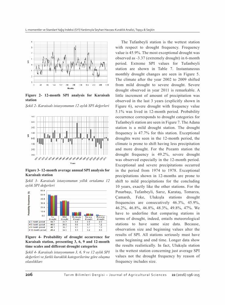
As shown in Table 5, most of the minimum SPI values are seen in 6-month (seasonal) time scale. The minimum SPI value of a month -3.76 (exceptionally drought) was experienced in Tomarza station for 6-months period in May 1989. One can see the SPI results and read from example following figures for the 12-month period of Karaisalı and Tufanbeyli stations, graphs for the other stations and explanations are not dwelled on because of their similarities. With reference to average monthly SPI values, the most severe drought station is the Karaisalı station, the maximum and minimum SPI values were observed as 3.59 (extremely wet) and -3.6 (extremely drought) respectively in 3-month period. Extreme SPI values for Karaisalı station are seen in Table 6. We can see the monthly flash drought and precipitation changes by reading SPI graph (Figure 2). Period 2005 to 2009 was moderate drought and mild drought. Especially year 2008 was severe drought (Figure 3). The drought frequency is 50.9% for this station. It means that drought incidents are experienced more than wet conditions
and happens more often. Moderate drought with frequency value 9.1% was observed in 12-month period. Probability occurrence corresponds to drought categories for Karaisalı station are seen in Figure 4.Table 5- The minimum SPI values of stationsÇizelge 5- İstasyonların minimum SPI değerleri
Station Minimum SPI Period Month YearAdana -3.18 6-month February 1973Çamardı -3.68 6-month June 1989Feke -3.2 3-month January 1973Karaisalı -3.6 3-month April 1989Karataş -3.74 6-month July 1989Pınarbaşı -3.75 6-month May 1989Sarız -3.39 9-month January 2001Pozantı -3 3-month April 1989Tomarza -3.76 6-month May 1989Tufanbeyli -3.37 6-month June 1989Ulukışla -3.3 6-month October 1984
Table 6- Extreme SPI values of droughts and precipitations for Karaisalı station, presenting 3, 6, 9 and 12-month time scalesÇizelge 6- Karaisalı istasyonunun 3, 6, 9 ve 12 aylık zaman serileri için ekstrem SPI değerleri
3-month period 6-month period 9-month period 12-month periodExceptional drought month April July October AprilObserved year 1989 1989 1989 2008SPI value -3.6 -2.98 -2.42 -2.15Exceptional wet month March June September DecemberObserved year 1994 1994 1994 1994SPI Value 3.59 3.42 3.45 3.31
The most severe yearin respect to the 2007 2008 2008 2008
average SPI valueSPI value -0.88 -1.36 -1.7 -1.84
The most wet yearin respect to the 1988 1994 1994 1994
average SPI valueSPI value 0.99 1.54 2.24 2.84
L-momentler ve Standart Yağış İndeksi (SYİ) Yardımıyla Seyhan Havzası Kuraklık Analizi, Topçu & Seçkin
206 Ta r ı m B i l i m l e r i D e r g i s i – J o u r n a l o f A g r i c u l t u r a l S c i e n c e s 22 (2016) 196-215
Figure 2- 12-month SPI analysis for Karaisalı stationŞekil 2- Karaisalı istasyonunun 12 aylık SPI değerleri
Figure 3- 12-month average annual SPI analysis for Karaisalı stationŞekil 3- Karaisalı istasyonunun yıllık ortalama 12 aylık SPI değerleri
Figure 4- Probability of drought occurrence for Karaisalı station, presenting 3, 6, 9 and 12-month time scales and different drought categoriesŞekil 4- Karaisalı istasyonunun 3, 6, 9 ve 12 aylık SPI değerleri ve farklı kuraklık kategorilerine göre oluşma olasılıkları
The Tufanbeyli station is the wettest station with respect to drought frequency. Frequency value is 45.9%. The most exceptional drought was observed as -3.37 (extremely drought) in 6-month period. Extreme SPI values for Tufanbeyli station are shown in Table 7. Instantaneous monthly drought changes are seen in Figure 5. The climate after the year 2002 to 2009 shifted from mild drought to severe drought. Severe drought observed in year 2011 is remarkable. A little increment of amount of precipitation was observed in the last 3 years (explicitly shown in Figure 6), severe drought with frequency value 5.1% was lived in 12-month period. Probability occurrence corresponds to drought categories for Tufanbeyli station are seen in Figure 7. The Adana station is a mild drought station. The drought frequency is 47.7% for this station. Exceptional droughts were seen in the 12-month period, the climate is prone to shift having less precipitation and more drought. For the Pozantı station the drought frequency is 49.2%, severe drought was observed especially in the 12-month period. Exceptional and severe precipitations occurred in the period from 1974 to 1978. Exceptional precipitations shown in 12-months are prone to shift to mild precipitations for the concluding 10 years, exactly like the other stations. For the Pınarbaşı, Tufanbeyli, Sarız, Karataş, Tomarza, Çamardı, Feke, Ulukışla stations drought frequencies are consecutively 46.3%, 45.9%, 46.2%, 46.8%, 46.8%, 48.3%, 49.8%, 47%. We have to underline that comparing stations in terms of drought, indeed, entails meteorological stations to have same size data. Because, observation size and beginning values alter the results of SPI. All stations seriously must have same beginning and end time. Longer data show the results realistically. In fact, Ulukışla station is the wettest station concerning just average SPI values not the drought frequency by reason of frequency includes size.

Drought Analysis of the Seyhan Basin by Using Standardized Precipitation Index (SPI) and L-moments, Topçu & Seçkin
207Ta r ı m B i l i m l e r i D e r g i s i – J o u r n a l o f A g r i c u l t u r a l S c i e n c e s 22 (2016) 196-215
Figure 5- 12-month SPI analysis for Tufanbeyli stationŞekil 5- Tufanbeyli istasyonunun 12 aylık SPI değerleri
Figure 6- 12-month average annual SPI analysis for Tufanbeyli stationŞekil 6- Tufanbeyli istasyonunun yıllık ortalama 12 aylık SPI değerleri
Figure 7- Probability of drought occurrence for Tufanbeyli station, presenting 3, 6, 9 and 12-month time scales and different drought categoriesŞekil 7- Tufanbeyli istasyonunun 3, 6, 9 ve 12 aylık SPI değerleri ve farklı kuraklık kategorilerine göre oluşma olasılıkları
The results also indicate that high elevation located stations have lower amount of precipitation, yet, because of the low temperature and sun energy, they have lowest evaporation rate so this engenders less drought events. Generally, all of the stations are on the boundary of drought. According to results, we can claim that the Seyhan Basin, average frequency of drought of the 11 stations considered, is neither drought nor wet but experiencing extreme event from time to time. Basin has the 47.7% frequency of occurrence of drought.
Table 7- Extreme SPI values of droughts and precipitations for Tufanbeyli station, presenting 3, 6, 9 and 12-month time scalesÇizelge 7- Tufanbeyli istasyonunun 3, 6, 9 ve 12 aylık zaman serileri için ekstrem SPI değerleri
3-month period 6-month period 9-month period 12-month periodExceptional drought month January June September OctoberObserved year 2001 1989 1989 2001SPI value -3.24 -3.37 -3.27 -2.6Exceptional wet month September November November JanuaryObserved year 2002 1996 1988 1989SPI Value 2.42 2.83 2.43 1.87The most severe yearin respect to the 1989 1989 2001 2001average SPI valueSPI value -1.35 -1.46 -1.78 -1.85The most wet yearin respect to the 1988 1988 1988 1988average SPI valueSPI value 1.09 1.26 1.4 1.47
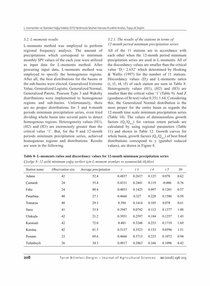
L-momentler ve Standart Yağış İndeksi (SYİ) Yardımıyla Seyhan Havzası Kuraklık Analizi, Topçu & Seçkin
208 Ta r ı m B i l i m l e r i D e r g i s i – J o u r n a l o f A g r i c u l t u r a l S c i e n c e s 22 (2016) 196-215
3.2. L-moments results
L-moments method was employed to perform regional frequency analysis. The amount of precipitations which correspond to minimum monthly SPI values of the each year were utilized as input data for L-moments method. After procuring input data, L-moments method was employed to specify the homogenous regions. After all, the best distributions for the basins or the sub-basins were elected. Generalized Extreme Value, Generalized Logistic, Generalized Normal, Generalized Pareto, Pearson Type 3 and Wakeby distributions were implemented to homogenous regions and sub-basins. Unfortunately, there are no proper distributions for 3 and 6-month periods minimum precipitation series, even tried dividing whole basin into several parts to detect homogenous regions. Heterogeneity values (H1), (H2) and (H3) are enormously greater than the critical value ‘1’. But, for the 9 and 12-month periods minimum precipitation series, achieved homogenous regions and distributions. Results are seen in the following.
3.2.1. The results of the stations in terms of 12-month period minimum precipitation series
All of the 11 stations are in accordance with each other when the 12-month period minimum precipitation series are used in L-moments. All of the discordancy values are smaller than the critical value ‘Di= 2.632’ which determined by Hosking & Wallis (1997) for the number of 11 stations. Discordancy values (Di) and L-moments ratios (t, t3, t4, t5) of each station are seen in Table 8. Heterogeneity values (H1), (H2) and (H3) are smaller than the critical value ‘1’ (Table 9). And Z (goodness-of fit test) value 0.35≤ 1.64. Considering this, the Generalized Normal distribution is the most proper for the entire basin as regards the 12-month time scale minimum precipitation series (Table 10). The values of dimensionless growth factors (QT/Qave) for various return periods are calculated by using regional parameters (Table 11) and shown in Table 12. Growth curves for whole basin, growth factors (QT/Qave) of best fitted distributions correspond to y (gumbel reduced values), are drawn in Figure 8.
Table 8- L-moments ratios and discordancy values for 12-month minimum precipitation seriesÇizelge 8- 12 aylık minimum yağış serileri için L-moment oranları ve uyumsuzluk ölçüleri
Station name Observation size Average precipitation t t 3 t 4 t 5 Di
Adana 42 52.4 0.4837 0.2637 0.125 0.078 0.62
Çamardı 24 35.4 0.4331 0.2441 0.119 -0.006 0.76
Feke 24 80.4 0.4053 0.1425 0.097 0.1201 0.57
Pınarbaşı 40 27.1 0.4666 0.327 0.228 0.1586 0.58
Tomarza 40 29.3 0.394 0.1414 0.105 0.078 0.61
Sarız 41 33.8 0.3947 0.0742 0.112 0.1377 1.88
Ulukışla 42 21.2 0.3951 0.2597 0.184 0.1257 1.43
Karaisalı 42 72.0 0.485 0.3248 0.253 0.1719 1.69
Karataş 42 81.5 0.5137 0.3523 0.153 0.0596 1.51
Pozantı 23 69.6 0.4666 0.3713 0.223 0.1072 0.94
Tufanbeyli 26 34.3 0.4917 0.2863 0.166 0.1096 0.42
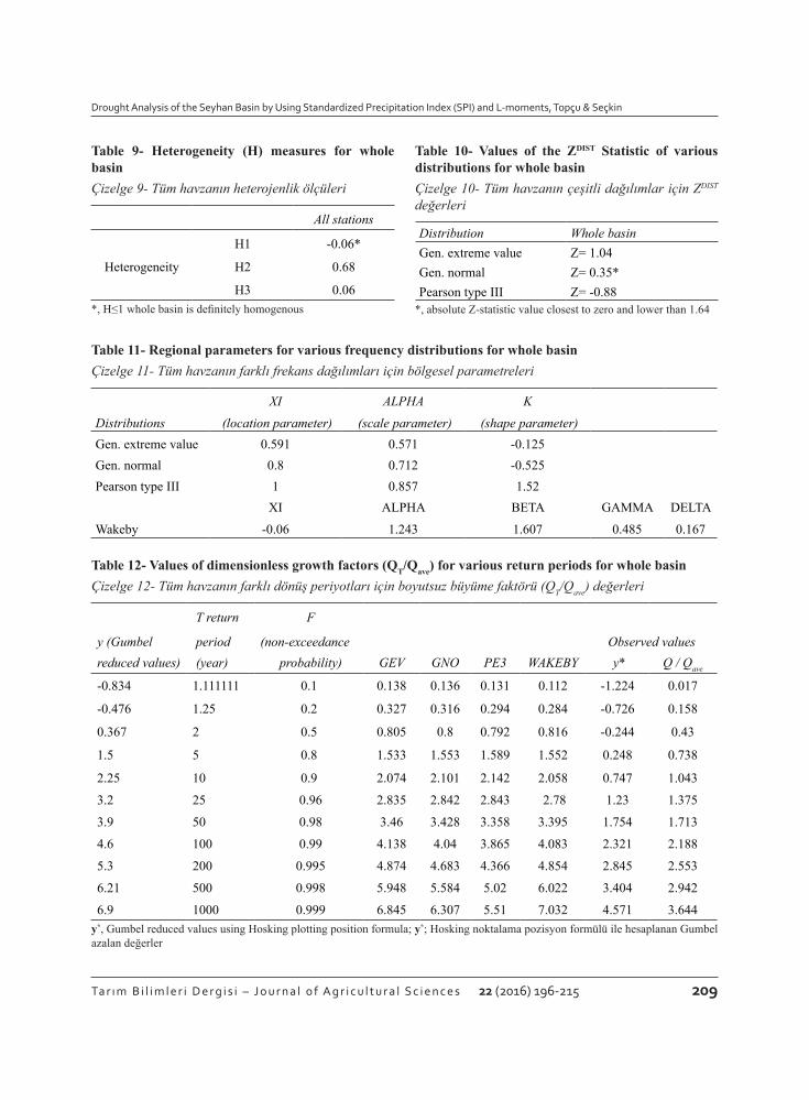
Drought Analysis of the Seyhan Basin by Using Standardized Precipitation Index (SPI) and L-moments, Topçu & Seçkin
209Ta r ı m B i l i m l e r i D e r g i s i – J o u r n a l o f A g r i c u l t u r a l S c i e n c e s 22 (2016) 196-215
Table 9- Heterogeneity (H) measures for whole basinÇizelge 9- Tüm havzanın heterojenlik ölçüleri
All stations
H1 -0.06*
Heterogeneity H2 0.68
H3 0.06*, H≤1 whole basin is definitely homogenous
Table 10- Values of the ZDIST Statistic of various distributions for whole basinÇizelge 10- Tüm havzanın çeşitli dağılımlar için ZDIST değerleri
Distribution Whole basinGen. extreme value Z= 1.04 Gen. normal Z= 0.35*Pearson type III Z= -0.88
*, absolute Z-statistic value closest to zero and lower than 1.64
Table 11- Regional parameters for various frequency distributions for whole basinÇizelge 11- Tüm havzanın farklı frekans dağılımları için bölgesel parametreleri
XI ALPHA K
Distributions (location parameter) (scale parameter) (shape parameter) Gen. extreme value 0.591 0.571 -0.125Gen. normal 0.8 0.712 -0.525Pearson type III 1 0.857 1.52
XI ALPHA BETA GAMMA DELTA
Wakeby -0.06 1.243 1.607 0.485 0.167
Table 12- Values of dimensionless growth factors (QT/Qave) for various return periods for whole basinÇizelge 12- Tüm havzanın farklı dönüş periyotları için boyutsuz büyüme faktörü (QT/Qave) değerleri
T return F
y (Gumbel period (non-exceedance Observed valuesreduced values) (year) probability) GEV GNO PE3 WAKEBY y* Q / Qave
-0.834 1.111111 0.1 0.138 0.136 0.131 0.112 -1.224 0.017
-0.476 1.25 0.2 0.327 0.316 0.294 0.284 -0.726 0.158
0.367 2 0.5 0.805 0.8 0.792 0.816 -0.244 0.43
1.5 5 0.8 1.533 1.553 1.589 1.552 0.248 0.738
2.25 10 0.9 2.074 2.101 2.142 2.058 0.747 1.043
3.2 25 0.96 2.835 2.842 2.843 2.78 1.23 1.375
3.9 50 0.98 3.46 3.428 3.358 3.395 1.754 1.713
4.6 100 0.99 4.138 4.04 3.865 4.083 2.321 2.188
5.3 200 0.995 4.874 4.683 4.366 4.854 2.845 2.553
6.21 500 0.998 5.948 5.584 5.02 6.022 3.404 2.942
6.9 1000 0.999 6.845 6.307 5.51 7.032 4.571 3.644y*, Gumbel reduced values using Hosking plotting position formula; y*; Hosking noktalama pozisyon formülü ile hesaplanan Gumbel azalan değerler
L-momentler ve Standart Yağış İndeksi (SYİ) Yardımıyla Seyhan Havzası Kuraklık Analizi, Topçu & Seçkin
210 Ta r ı m B i l i m l e r i D e r g i s i – J o u r n a l o f A g r i c u l t u r a l S c i e n c e s 22 (2016) 196-215
Figure 8- Growth curves for the whole basinŞekil 8- Tüm havza için büyüme eğrileri
3.2.2. The results of region 1 and region 2 in terms of 9-month period minimum precipitation seriesTwo homogenous regions are procured by dividing basin, by selecting stations with respect to approximate elevation values, as Region 1 and
Region 2 for 9-month period minimum precipitation series. Discordancy values (Di) and L-moments ratios (t, t3, t4, t5) of region 1 and region 2 are seen in Table 13 and Table 14. Heterogeneity values (H1), (H2) and (H3) are smaller than the critical value ‘1’ for all regions (Table 15). Also Z (goodness-of fit test) values -0.88≤1.64 and 0.57≤1.64 for region 1 and 2 respectively. The Pearson Type 3 distribution is the most proper for two homogenous sub-basins as regards the 9-month time scale minimum precipitation series (Table 16). The values of dimensionless growth factors (QT/Qave) for various return periods are calculated by using regional parameters (Table 17) and shown in Table 18 and Table 19 for region 1 and region 2 respectively. Growth curves, growth factors (QT/Qave) of best fitted distributions correspond to y (gumbel reduced values), are drawn in Figure 9 for region 1 and Figure 10 for region 2.
Table 13- L-moments ratios and discordancy values for region 1Çizelge 13- Bölge 1’in L-moment oranları ve uyumsuzluk değerleri
Region 1Station name Observation size Average precipitation t t 3 t 4 t 5 DiAdana 42 47.3 0.477 0.2348 0.1099 0.0828 1.09Feke 24 82.5 0.4594 0.2416 0.1041 0.0775 0.51Karaisalı 42 63.9 0.4538 0.2627 0.203 0.1666 1.12Karataş 42 41.6 0.522 0.301 0.1485 0.0882 1.18Pozantı 23 58.1 0.3867 0.2211 0.1559 0.0911 1.1
Table 14- L-moments ratios and discordancy values for region 2Çizelge 13- Bölge 1’in L-moment oranları ve uyumsuzluk değerleri
Region 2
Station name Observation size Average precipitation t t 3 t 4 t 5 Di
Çamardı 24 33 0.3365 0.156 0.1864 0.0494 1.26
Pınarbaşı 40 22.2 0.4081 0.158 0.1212 0.1103 0.32
Tomarza 40 25.6 0.3259 0.211 0.1423 0.0338 1.27
Sarız 41 29.8 0.3908 0.083 0.0617 0.0635 1.54
Ulukışla 42 16.6 0.3838 0.224 0.1391 0.0421 0.42
Tufanbeyli 26 39.6 0.4765 0.197 0.0682 0.0764 1.2
Drought Analysis of the Seyhan Basin by Using Standardized Precipitation Index (SPI) and L-moments, Topçu & Seçkin
211Ta r ı m B i l i m l e r i D e r g i s i – J o u r n a l o f A g r i c u l t u r a l S c i e n c e s 22 (2016) 196-215
Table 15- Heterogeneity (H) measures for region 1 and region 2Çizelge 15- Bölge 1 ve Bölge 2’nin heterojenlik ölçüleri
Region 1 Region 2
H1 -0.21* 0.59*
Heterogeneity H2 -1.5 -0.23
H3 -1.45 -0.94*, H≤1 sub-regions are definitely homogenous
Table 16- Values of the ZDIST Statistic of various distributions for region 1 and region 2Çizelge 16- Tüm havzanın çeşitli dağılımlar için ZDIST değerleri
Distribution Region 1 Region 2Gen. extreme value Z= 1.25 Z= 1.33Gen. normal Z= 0.77 Z= 1.13Pearson type III Z= -0.08* Z= 0.57*Gen. pareto Z= -1.12
*, absolute Z-statistic values closest to zero and lower than 1.64
Table 17- Regional parameters for various frequency distributions in sub-regions 1 and 2Çizelge 17- Alt bölgeler 1 ve 2’nin farklı frekans dağılımları için bölgesel parametreleri
XI ALPHA K
Region Distributions (location
parameter) (scale
parameter) (shape
parameter) Gen. extreme value 0.573 0.589 -0.131Gen. normal 0.789 0.736 -0.534
Region 1 Pearson type III 1 0.893 1.545Gen. pareto -0.021 1.208 0.183
XI ALPHA BETA GAMMA DELTAWakeby -0.058 1.345 0.546 0.093 0.508Gen. extreme value 0.679 0.554 -0.002Gen. normal 0.882 0.648 -0.353
Region 2 Pearson type III 1 0.705 1.039XI ALPHA BETA GAMMA DELTA
Wakeby -0.021 1.467 2.94 0.71 -0.095
Table 18- Values of dimensionless growth factors (QT/Qave) for various return periods in Region 1Çizelge 18- Bölge 1’in farklı dönüş periyotları için boyutsuz büyüme faktörü (QT/Qave) değerleri
y (Gumbel reduced values) -0.834 -0.476 0.367 1.5 2.25 3.2 3.9 4.6 5.3 6.21 6.9
T return period (year) 1.1111 1.25 2 5 10 25 50 100 200 500 1000
F (non-exceedance probability) 0.1 0.2 0.5 0.8 0.9 0.96 0.98 0.99 0.995 0.998 0.999
GPA 0.105 0.243 0.765 1.663 2.249 2.918 3.355 3.739 4.078 4.465 4.718GEV 0.108 0.301 0.794 1.549 2.114 2.912 3.572 4.289 5.072 6.22 7.184GNO 0.105 0.29 0.789 1.571 2.143 2.921 3.538 4.185 4.865 5.82 6.589PE3 0.101 0.267 0.78 1.61 2.188 2.922 3.463 3.996 4.522 5.211 5.727WAKEBY 0.09 0.246 0.795 1.613 2.109 2.733 3.262 3.916 4.778 6.427 8.262y* -1.219 -0.763 -0.281 0.242 0.743 1.21 1.737 2.325 2.844 3.421 4.55Q / Qave 0.004 0.112 0.349 0.736 1.042 1.383 1.776 2.186 2.638 3.007 3.64
y*, Gumbel reduced values using Hosking plotting position formula; y*, Hosking noktalama pozisyon formülü ile hesaplanan Gumbel azalan değerler
L-momentler ve Standart Yağış İndeksi (SYİ) Yardımıyla Seyhan Havzası Kuraklık Analizi, Topçu & Seçkin
212 Ta r ı m B i l i m l e r i D e r g i s i – J o u r n a l o f A g r i c u l t u r a l S c i e n c e s 22 (2016) 196-215
Figure 9- Growth curves for region 1Şekil 9- Bölge 1 için büyüme eğrileri
Figure 10- Growth curves for region 2Şekil 10- Bölge 2 için büyüme eğrileri
4. ConclusionsTurkey is in the temperate (semi-arid) zone of the world. Due to its geographical change in short distance, there are various climate types. Some parts (northeast) are exceptionally wet but some parts (central south) severe drought. These circumstances affect, no doubt, the whole country economically, agriculturally, culturally and socially. The Standardized Precipitation Index identified the drought conditions realistically for the specific 3, 6, 9 and 12-month time scales. Probing the drought for 4 different time scales provides us tracing the bad or good impacts of the drought or excessive precipitations on water resources, reservoirs and underground water in the Seyhan Basin. Considering the output data, severe and extreme drought mostly experienced for 6-month time scale. SPI showed the pattern of drought of 11 stations in the Seyhan Basin successfully and unfolded the years have flash climatic changes, keeping in view monthly precipitation alteration. L-moments method was exploited to have probable minimum precipitations which will create drought. We can readily attain the minimum amount of precipitation correspond
Table 19- Values of dimensionless growth factors (QT/Qave) for various return periods in Region 2Çizelge 19- Bölge 2’nin farklı dönüş periyotları için boyutsuz büyüme faktörü (QT/Qave) değerleri
T return period (year)
F (non-exceedance
probability)y (Gumbel reduced
values)Observed values
GEV GNO PE3 WAKEBY y* Q / Qave
-0.834 1.11111 0.1 0.217 0.215 0.21 0.187 -1.228 0.055-0.476 1.25 0.2 0.415 0.411 0.4 0.376 -0.793 0.2160.367 2 0.5 0.882 0.882 0.88 0.889 -0.289 0.4941.5 5 0.8 1.511 1.517 1.531 1.533 0.254 0.82.25 10 0.9 1.929 1.931 1.946 1.946 0.75 1.1293.2 25 0.96 2.457 2.451 2.447 2.447 1.245 1.3983.9 50 0.98 2.85 2.835 2.805 2.798 1.77 1.7024.6 100 0.99 3.24 3.217 3.15 3.127 2.318 1.9665.3 200 0.995 3.63 3.601 3.485 3.435 2.846 2.2066.21 500 0.998 4.144 4.114 3.916 3.812 3.39 2.3196.9 1000 0.999 4.534 4.508 4.236 4.076 4.589 2.851
y*, Gumbel reduced values using Hosking plotting position formula; y*, Hosking noktalama pozisyon formülü ile hesaplanan Gumbel azalan değerler

Drought Analysis of the Seyhan Basin by Using Standardized Precipitation Index (SPI) and L-moments, Topçu & Seçkin
213Ta r ı m B i l i m l e r i D e r g i s i – J o u r n a l o f A g r i c u l t u r a l S c i e n c e s 22 (2016) 196-215
to requested return periods by using growth factor values multiplied by average precipitation. These data should be put into cognizance by farmers, politicians and water resource planners even citizens, consequently, the data may be used for other basins having the same climatologic characters throughout the world. For further researches precipitation values should not singly be used for monitoring drought, because occurrence of drought cannot be explained by only lack of precipitation. Urbanization and housing, vegetation condition, reservoir storage, number of snowy days, number of days without rain, wind direction, solar radiation, day length and duration of insolation, air temperature and humidity also affect occurrence of drought. For this reason all these factors, at least some of them must be combined during analysis and calculation drought.
The Mediterranean region, including the Seyhan Basin, is detected as the most vulnerable to global warming (IPCC 2007). Scientists on this point say that temperature in this basin would increase about 2-3.5 °C until the end of this century (CSB 2011). Rising temperature accelerates the rate of evaporation, principally, from the beginning of the 2000s till now, as results show, there was a considerable decline in the amount of precipitations. The worst of all, the Seyhan Basin is going through not only decrease in precipitations but also increase in temperatures and more frequent drought events. If these drivers come together too often, it could worsen the climatic situation already irresolute. Whether it is human induced or complexity of the atmosphere itself, unluckily global warming threatens the world, needless to say our study area ‘the Seyhan Basin’. We can see the flash or creeping alteration of precipitations from graphs. Serious precautions must be taken before colossal disasters emerge.
ReferencesAbolverdi J & Khalili D (2010). Probabilistic analysis
of extreme regional meteorological droughts by L-Moments in a semi-arid environment. Theoretical and Applied Climatology 102: 351-366
Altın B T & Barak B (2012). Seyhan Havzasında 1970-2009 yılları arasında yağış ve hava sıcaklığı
değerlerindeki değişimler ve eğilimler. Türk Coğrafya Dergisi 58: 21-34
Anlı S A, Apaydın H & Öztürk F (2009). Trabzon ilinde gözlenen yıllık maksimum yağışların bölgesel frekans analizi. Tarım Bilimleri Dergisi-Journal of Agricultural Sciences 15(3): 240-248
Anlı S A (2014). Güneydoğu anadolu bölgesinde referans bitki su tüketiminin (et0) zamansal değişimi ve rdi (keşif kuraklık indeksi) yöntemiyle meteorolojik kuraklık analizi. Tarım Bilimleri Dergisi-Journal of Agricultural Sciences 20(3): 248-260
Aydogan D, Kankal M & Önsoy H (2014). Regional flood frequency analysis for Çoruh Basin of Turkey with L-moments approach. Journal of Flood Risk Management doi: 10.1111/jfr3.12116
Blain C G (2012). Monthly values of the standardized precipitation index in the State of Sao Paulo, Brazil: Trends and spectral features under the normality assumption. Bragantia 71(1): 122-131
CSB (2011). Turkey’s National Climate Change Adaptation Strategy and Action Plan, T.R. Ministry of Environment and Urbanization, November 2011. Ankara (1st edition) http://www.csb.gov.tr/db/iklim/editordosya/Adaptation_Strategy.pdf (Access Date 03.03.2014)
Dalrymple T (1960). Flood Frequency Methods. U. S. Geol. Survey, Water Supply Paper 1453 A, Washington, 11-51
Dodangeh S, Sattari M T & Seçkin N (2011). Minimum akımların L momentler yöntemi ile bölgesel frekans analizi. Tarım Bilimleri Dergisi-Journal of Agricultural Sciences 17: 43-58
Dubey A (2014). Regional flood frequency analysis utilizing L-moments: A case study of Narmada Basin. International Journal of Engineering Research and Applications 4(2): 155-161
Dutra E, Giuseppe D F, Wetterhall F & Pappenberger F (2013). Seasonal forecasts of droughts in African Basins using the standardized precipitation index. Hydrology and Earth System Sciences 17: 2359-2373
Edwards D C & McKee T B (1997). Characteristics of 20th century drought in the United States at multiple time scales. Climatology Report Number 97-2, Colorado State University, Fort Collins, Colorado
Eslamian S S & Feizi H (2006). Maximum monthly rainfall analysis using L-moments for an arid region in isfahan province, Iran. Journal of Applied Meteorology and Climatology 46: 494-503
L-momentler ve Standart Yağış İndeksi (SYİ) Yardımıyla Seyhan Havzası Kuraklık Analizi, Topçu & Seçkin
214 Ta r ı m B i l i m l e r i D e r g i s i – J o u r n a l o f A g r i c u l t u r a l S c i e n c e s 22 (2016) 196-215
Eslamian S, Hassanzadeh H, Abedi-Koupai J & Gheysari M (2012). Application of L-moments for regional frequency analysis of monthly drought indexes. Journal of Hydrologic Engineering 17(1): 32-42
Fang Y, Mauzerall D L, Liu J, Fiore A M & Horowitz L W H (2013). Impacts of 21st century climate change on global air pollution-related premature mortality. Climatic Change 121: 239-253
Fowler H J & Kilsbyc G (2003). A regional frequency analysis of United Kingdom extreme rainfall from 1961 to 2000. International Journal of Climatology 23: 1313-1334
Fujihara Y, Simonovic P S, Topaloğlu F, Tanaka K & Tsugihiro W (2008). An inverse modelling approach to assess the impacts of climate change in the Seyhan River Basin, Turkey. Hydrological Sciences Journal 53(6): 1121-1136
Gebeyehu A (1989). Regional Flood Frequency Analysis. The Royal Institute of Technology, Stockholm, Sweden, Bulletin No. TRIVA-VBI-148
Gingras D & Adamowski K (1994). Performance of L-moments and nonparametric flood frequency analysis. Canadian Journal of Civil Engineering 21(5): 856-862
Guenang M G & Kamga M F (2014). Computation of the standardized precipitation index (spi) and its use to assess drought occurrences in cameroon over recent decades. Journal of Applied Meteorology and Climatology 53: 2310-2324
Gurkan D (2005). Assessment of Climate Change Impacts on Surface Water Resources in Seyhan River Basin. MSc, Thesis, Hacettepe University (in Turkish, unpublished)
Guttman N B (1998). Comparing the palmer drought severity index and the standardized precipitation index. Journal of the American Water Resources Association 34(1): 113-121
Guttman N B (1999). Accepting the Standardized Precipitation İndex: A Calculation Algorithm. Journal of the American Water Resources Association 35: 311-322
Hosking J R M (1986). The Theory of Probability Weighted Moments. Research Rep. RC 12210, 160 pp. IBM Research Division, Yorktown Heights, NY
Hosking J R M (1990). L-moments: Analysis and estimation of distributions using linear combinations of order statistics. Journal of the Royal Statistical Society 52(2): 105-124
Hosking J R M & Wallis J R (1993). Some statistics useful in regional frequency analysis. Water Resources Research 29(2): 271-281
Hosking J R M & Wallis J R (1997). Regional Frequency Analysis: An Approach Based on L-Moments. Cambridge University Press, UK
IPCC (2007). Intergovernmental Panel on Climate Change. http://www.ipcc.ch/ (Access Date 03.03.2014)
Jha S, Sehgal K V, Raghava R & Sinha M (2013). Trend of standardized precipitation index during Indian summer monsoon season in agro climatic zones of India. Earth System Dynamics Discussions 4: 429-449
Keskin F & Sorman A Ü (2010). Assessment of the Drought Pattern Change in Çamlıdere Basin Using SPI. BALWOİS 2010, 25-29 May Ohrid, Republic of Macedonia
Kömüscü A Ü (2001). An analysis of recent drought conditions in Turkey in relation to circulation patterns. Drought Network News (1994-2001). Paper 22
Landwehr J M, Matalas N C & Wallis J R (1979a). Probability weighted moments compared with some traditional techniques in estimating gumbel parameters and quantiles. Water Resources Research 15(5): 1055-1064
Landwehr J M, Matalas N C & Wallis J R (1979b). Estimation of parameters and quantiles of wakeby distributions. 1. Known lover bounds. Water Resources Research 15(6): 1361-1372
Landwehr J M, Matalas N C & Wallis J R (1979c). Estimation of parameters and quantiles of wakeby distributions. 1. Unknown lover bounds. Water Resources Research 15(6): 1373-1379
Li W, Fu R, Juarez R I N & Fernandes K (2008). Observed change of the standardized precipitation index, its potential cause and implications to future climate change in the amazon region. Philosophical Transactions of the Royal Society 363: 1767-1772
Lloyd-Hughes B & Saunders M A (2002). A drought climatology for Europe, International Journal of Climatology 22: 1571-1592
McKee T B, Doesken N J & Kleist J (1993). The Relationship of Drought Frequency and Duration to Time Scales. Reprints, 8th Conference on Applied Climatology, Anaheim, CA, USA, 179-184 pp
McRoberts B D & Nielsen-Gammon W J (2012). The use of a high-resolution standardized precipitation index for drought monitoring and assessment. Journal of Applied Meteorology and Climatology 51: 68-83
Drought Analysis of the Seyhan Basin by Using Standardized Precipitation Index (SPI) and L-moments, Topçu & Seçkin
215Ta r ı m B i l i m l e r i D e r g i s i – J o u r n a l o f A g r i c u l t u r a l S c i e n c e s 22 (2016) 196-215
NASA (2010a). Is Current Warming Natural? http://earthobservatory.nasa.gov/Features/ (Access Date: 03.03.2014)
NASA (2010b). Satellites Pinpoint Drivers of Urban Heat Islands in the Northeast. http://www.nasa.gov/topics/earth/features/heat-island (Access Date: 03.03.2014)
Norbiato D, Borga M, Sangati M & Zanon F (2007). Regional frequency analysis of extreme precipitation in the Eastern Italian Alps in the August 29, 2003 flash flood. Journal of Hydrology 345: 149-166
Parida B P & Moalafhi D B (2008). Regional rainfall frequency analysis for botswana using l-moments and radial basis function network. Physics and Chemistry of the Earth 33: 614-620
Saf B (2009). Regional flood frequency analysis using l moments for the Buyuk and Kucuk Menderes river basins of Turkey. Journal of Hydrologic Engineering 14(8): 783-794
Seckin N & Yurtal R (2008). L-momentlere dayalı göstergesel metodu ile bölgesel taşkın frekans analizi. Ç.Ü. Fen Bilimleri Dergisi 19: 120-129
Seckin N, Yurtal R, Haktanır T & Doğan A (2010a). Comparison of probability weighted moments and maximum likelihood methods used in flood frequency analysis for Ceyhan River Basin. The Arabian Journal for Science and Engineering 35(1): 49-69
Seckin N, Yurtal R, Haktanır T & Topaloğlu F (2010b). Regional flood frequency analysis of Ceyhan River Basin in Turkey using L-moments method. Fresenius Environmental Bulletin 19(11a): 2616-2624
Seckin N, Haktanır T & Yurtal R (2011). Flood frequency analysis of Turkey using L-moments method. Hydrological Processes 25: 3499
Selek B & Tuncok K I (2014). Effects of climate change on surface water management of Seyhan Basin, Turkey. Environmental and Ecological Statistics 21(3): 391-409
Sen B, Topcu S, Giorgi F, Bi X, Kanıt E.G & Dalkılıç T (2008). Seyhan Havzasında iklim değişikliğinin tarımsal su kullanımına etkileri. TMMOB 2. Su Politikaları Kongresi 20-22 Mart 2008, Ankara
Shi P, Chen X, Qu S, Zhang Z & Ma J (2010). Regional frequency analysis of low flow based on l moments: case study in karst area, southwest china. Journal of Hydrologic Engineering 15(5): 370-377
Simsek O & Cakmak B (2010). Drought analysis for 2007-2008 agricultural year of Turkey. Journal of Tekirdag Agricultural Faculty 7(3): 99-109
Stedinger J R, Vogel R M & Foufoula-Georgiou E (1993). Frequency Analysis of Extreme Events. Handbook of Hydrology D. R. Maidment, ed., McGraw-Hill Book Co., Inc., New York, NY
Tallaksen C Y, Ngongondo C S, Xu L, Alemaw B & Chirwa T (2011). Regional frequency analysis of rainfall extremes in southern malawi using the index rainfall and l-moments approaches. Stochastic Environmental Research and Risk Assessment 25(7): 939-955
Thom H C S (1951). A Frequency Distribution for precipitation (abstract). Bulletin of the American Meteorological Society 32(10): 397
Thom H C S (1958). A Note on the Gamma Distribution. Monthly Weather Review 86: 117-122
Tonkaz T (2006). Spatio-temporal assessment of historical droughts using SPI with GIS in GAP Region, Turkey. Journal of Applied Sciences 6(12): 2565-2571
Topcu E (2013). L-Momentler ve Standart Yağış İndeksi (SYİ) yardımıyla Seyhan Havzası Kuraklık Analizi. Yüksek lisans tezi, Çukurova Üniversitesi Fen Bilimleri Enstitüsü, Adana
Trenberth K E & Dai A (2007). Effects of Mount Pinatubo volcanic eruption on the hydrological cycle as an analog of geoengineering. Geophysical Research Letters 34: L15702
Türkes M (1999). Vulnerability of Turkey to desertification with respect to precipitation and aridity conditions. Turkish Journal of Engineering and Environmental Science 23: 363-380
Vardiman L (2008). A new theory of climate change. Acts & Facts 37(11): 10
Wilhite D & Glantz M R (1987). Understanding the drought phenomenon. The role of definitions, in Wilhite, David, Easterling, William and Wood, David eds, Planning for drought: Boulder, Colo. Westview Press pp. 11-27
WMO (2007). Global Climate Highlights in 2006. http://www.wmo.int/pages/ (Access Date: 03.03.2014)
Xie H, Ringler C, Zhu T & Waqas A (2013). Droughts in Pakistan: A spatiotemporal variability analysis using the standardized precipitation index. Water International 38(5): 620-631