drag and momentum fluxes produced by mountain waves
TRANSCRIPT

UNIVERSITY OF READING
Department of Mathematics
Drag and Momentum Fluxes Produced byMountain Waves
By
Yu Chau Lam
Supervisor: Dr. Miguel Teixeira
A dissertation submitted in partial fulfillment of the requirements for the degree of
MSc in Mathematical and Numerical Modeling of the Atmosphere and Oceans
October 2013


Declaration
I confirm that this is my own work, and the use of all material from other sources has beenproperly and fully acknowledged.
Signed .................................................
Yu Chau Lam
October 2013
i

Abstract
Orographically generated gravity waves, being a sub-grid scale process that has a great im-
pact on numerical weather prediction, must be parametrized in large-scale atmospheric models
(Lott and Miller (1997); Gregory et al. (1998)). Since the 1990s, most of the existing drag
parametrization schemes are based on linear hydrostatic theory, while non-hydrostatic effects
have been studied mainly using numerical simulations, as in the study by Kim and Arakawa
(1995). Although the effects of critical levels (levels where waves are attenuated and absorbed)
have been noted and studied since the 1950s, their three-dimensional filtering effects due to
directional wind shear have been drawing the attention of meteorologists only from the last 20
years onwards (Shutts 1995). Such directional filtering effects contribute to the formation of a
critical layer, in which each level is a critical level for a certain wave number (Broad (1995);
Shutts (1995)). Moreover, non-hydrostatic effects in conjunction with such critical layers have
not been studied thoroughly.
In this dissertation, various approaches, including solving for exact analytic solution, numerical
methods and the WKB approximation, are adopted to solve the Taylor-Goldstein equation, for
flow over a 3D isolated mountain, in both hydrostatic and non-hydrostatic conditions, under
the assumption of inviscid, non-rotating, linearized flow with the Boussinesq approximation.
Two wind profiles with directional shear are chosen to investigate the 3D directional filtering
effect of critical layers. Calculation results mainly focus on two relevant physical quantities,
namely the surface drag, which defines the total vertical flux of horizontal momentum of the
mean wind available to be transported upward (Teixeira et al. (2004)), and the momentum
fluxes, whose divergence corresponds to a force acting on the atmosphere that decelerates the
mean wind (Teixeira and Miranda (2009)).
The main findings show that as the system enters the non-hydrostatic regime, the variation
of those two quantities with the Richardson number Ri (which is defined to be the static sta-
bility N2 of the atmosphere divided by the square of wind shear) becomes more non-linear
and dependent on the degree of non-hydrostaticity. Moreover, a significant decrease in mag-
nitude of the two quantities can be observed, which is due to wave reflection effects. Such a
drop in magnitude may cause an overestimation of the surface drag and momentum fluxes in
parametrization schemes where the hydrostatic assumption is made. Therefore, the inclusion
of non-hydostatic effects should be able to improve the performance of current parametrization
schemes for orographically generated gravity waves.
ii

Acknowledgments
First and foremost, I would like to take this opportunity to thank my parents for their love and
nuture all along, which guide me to fight for my dream and lead to all the achievements I have
today.
Second, I would like to express my gratitude to my supervisor Dr. Miguel Teixeira for his
precious guidance and scientific insight, which is indispensable for the accomplishment of this
dissertation. Moreover, I treasure the valuable discussion with Prof. Mike Baines, whose
encouragement helped me overcome a lot of difficulties encountered during this dissertation.
Third, I would like to thank my friends, especially Mr. Tsz Kin Lai Eric and Ms. Na Zhou Jody,
for their yearlong support and care. We accompanied to face all the challenges throughout this
entire year. Cheers to our friendship.
iii

Contents
Declaration i
Abstract ii
Acknowledgments iii
Contents iv
List of symbols vi
1 Introduction 1
1.1 Aims and Outline of this thesis 2
1.2 Basic Wave properties 3
1.2.1 The wave phase and phase velocity 3
1.2.2 The group velocity and the dispersion relation 5
1.3 Linear Theory 6
1.3.1 The Boussinesq approximation and Linearization 6
1.3.2 The Taylor-Goldstein equation 8
2 Flow over a 2-D isolated mountain 10
2.1 Mountain profile 10
2.2 Different regimes of solution 11
2.3 The surface drag and momentum fluxes: conceptually 14
2.4 The surface drag and momentum fluxes: mathematically 16
2.5 Height dependent Scorer Parameter 17
2.5.1 The critical level 18
3 Flow Over a 3-D Isolated Mountain in the Hydrostatic Regime 20
3.1 Setting of the problem 20
3.1.1 The critical layer 21
3.1.2 The wind profiles 21
3.1.3 The mountain profile 22
3.2 Methodology 23
3.2.1 Exact solution for linear wind profile in hydrostatic limit 23
3.2.2 A Linear numerical model 24
iv
3.2.3 The WKB approximation 26
3.3 Results and comparison 33
3.3.1 Linear wind profile 35
3.3.2 Turning wind profile 37
4 Flow Over a 3-D Isolated Mountain in the Non-hydrostatic Regime 39
4.1 Identification of the non-hydrostatic regime 40
4.2 The linear wind profile with directional shear - Analytic solution 40
4.2.1 Results and discussion 47
4.3 The turning wind profile 50
4.3.1 A two-layer atmosphere 50
4.3.2 Numerical method 51
4.3.3 Boundary conditions 52
4.3.4 Results and discussion 55
5 Concluding remarks and future work 58
5.1 Analysis of methods 58
5.2 Calculation results 59
5.2.1 Hydrostatic regime 59
5.2.2 Non-hydrostatic regime 59
5.3 Overall effect of non-hydrostaticity 60
5.4 Future work 60
Bibliography 62
Appendices 65
A Behavior of gravity waves near a critical level 65
B Definition of Fourier integrals and the Parseval Theorem 71
v

List of symbols
κ = (k1, k2, k3) 3D total wave vector
k = (k1, k2, 0) Horizontal projection of κ (referred as horizontal wave )
k12 The magnitude of k
ω Angular frequency
vp = (vp1, vp2, vp3) 3D phase velocity
vg = (vg1, vg2, vg3) 3D group velocity
u = (u, v, w) Full velocity of the wind
f The Coriolis parameter
p Pressure
θ Potential temperature
ρ Density of air
T Temperature
g Magnitude of gravitational acceleration
Rd Ideal gas constant for dry air
N The Brunt-Vaisala frequency
Ω The Doppler-shifted intrinsic frequency
m The vertical wave number
L The inverse of m
q The Fourier transform of the quantity q, unless otherwise specified
h The orography profile
hm The height scale of the orography
a The width scale of the orography
a Non-dimensionalized width scale of the orography
η Vertical streamline displacement
l The Scorer parameter
Ri The Richardson number
vi

Chapter 1
Introduction
A stably stratified atmosphere has the important property of supporting the propagation of
waves with different scales, from the large-scale planetary waves such as Rossby waves to the
small-scale sound waves. Some of these waves play a crucial role in meteorological phenonema
(e.g. Rossby waves), while others do not (e.g. sound waves). Nowadays, with the ever improving
technology, numerical weather prediction plays an increasingly important role in weather fore-
cast. However, no matter how advanced the modern meteorological models are, there are still
many phenomena that they cannot capture, for example small-scale but important processes
like convection, cloud microphysics, turbulence, etc. The subject of this study, terrain-generated
gravity waves, are also one of these processes. These small-scale processes can only be captured
by parametrization schemes, and therefore a deep understanding of them is necessary in order
to develop good parametrizations.
As their name tells, terrain-generated gravity waves are wave phenomena generated by orog-
raphy. One distinctive feature of terrain-generated gravity-waves is that they are stationary
to observers on the ground (Lin (2007); Nappo (2012)). From the foregoing discussion we
will learn that these waves are non-dispersive since all wave components have the same phase
speed, which is 0. Terrain-generated gravity waves are worth studying since their presence acts
to transport horizontal momentum of the mean flow vertically. As the waves propagate upward
to a certain high level, they may break and generate turbulence, which is known as clear-air
turbulence (CAT) (Nappo 2012). Studies have shown that such wave-breaking zones often co-
incide with critical levels (Grubisic and Smolarkiewicz (1997); Shutts and Gadian (1999)). The
detailed behavior of gravity waves in the vicinity of critical levels will be studied in chapter 2
and appendix A.
There are mainly two kinds of terrain-generated gravity waves, namely vertically-propagating
mountain waves and trapped lee waves (Nappo 2012). One significant difference between them
is that trapped lee waves appear only on the downwind side of mountains. As will be discussed
in later chapters, the atmosphere may sometimes be unable to support wave propagation for
certain waves at some levels. As such waves propagate upward from the obstacle, wave reflec-
tion will occur and cause the waves to be trapped in the lower atmosphere and extend only
horizontally (Nappo 2012). As a result, such waves usually have less impact on the high atmo-
1

sphere.
Different from trapped lee waves, vertically propagating mountain waves can extend both hor-
izontally and vertically, and hence have a much greater impact on the high atmosphere, since
transport of momentum and energy can reach much higher levels. In fact, mountain waves even
play an important role in modulating the atmospheric global circulation (McFarlane (1987);
Teixeira and Miranda (2004)).
1.1 Aims and Outline of this thesis
Orographically generated gravity waves influence the atmosphere by exerting a drag force on
it, which acts to decelerate the mean flow. At the same time, horizontal momentum associated
with the mean flow is transported upward to the upper atmosphere. These processes are of
small scale and common in the atmosphere. In order to produce accurate numerical weather
predictions, such small-scale processes must be parametrized in large-scale meteorological mod-
els, due to the lack of sufficient resolution to capture their details. Parametrizations of these
processes have to be developed by first studying their detailed dynamics in idealized settings
and summarizing the variation of quantities that have an important impact on the atmosphere.
The main aim of this dissertation is to study the variations of important quantities associ-
ated with the mountain waves, such as the surface drag and momentum fluxes for flow over
an idealized 3D isolated mountain, subject to different wind profiles, in both hydrostatic and
non-hydrostatic conditions. Non-hydrostatic effects associated with the wind profile will be
examined to see how they affect the variation of those relevant quantities. This is practically
important since the current parametrization schemes assume a hydrostatic atmosphere, which
is certainly not always valid. Moreover, these wind profiles are designed specifically for investi-
gating the interactions between the gravity waves and critical levels, where the wave energy is
known to be significantly absorbed and wave breaking may easily occur (Broad (1995); Shutts
(1995)).
In this chapter, most of the basic concepts, which are necessary for the discussion in the later
chapters, will be introduced. Those concepts include the group velocity and the dispersion
relation of the gravity waves, as well as the linear theory, which uses the important Boussi-
nesq approximation, and the derivation of the Taylor Goldstein equation. In fact, solving the
Taylor-Goldstein equation subject to different types of flow is the main target of this study,
since all the information required can be obtained from the solution to this equation.
In chapter 2, an example using a 2D mountain ridge and a constant wind profile will be il-
lustrated, which allows us to classify the different regimes of the solution space of the Taylor-
Goldstein equation. The discussion in the later chapters will be based on this classification.
Next, two important quantities will be introduced, namely the surface drag and the vertical
momentum fluxes. The discussion will first explain the physical meaning of these quantities by
looking at a 2D mountain ridge example, and then give their mathematical formulations.
Chapter 3 and 4 contain the main results of this study, which are divided into the hydrostatic
2
and non-hydrostatic limits. Different approaches have been used in each limit, such as deriving
exact analytic solutions, use of the WKB approximation, and different numerical approaches.
The main calculation results and discussion will focus on the surface drag and the momentum
fluxes.
Chapter 5 summarizes the main findings of this study and states some of the unsolved problems
and future work.
1.2 Basic Wave properties
Most of the wavy oscillations observed in nature do not just consist of a single wave, but are
usually an overlap of a band of waves. Therefore, the analysis of how waves overlap and interact
to form the observed propagating oscillations will be of great importance for understanding wave
phenomena. In this section, some general properties of plane waves will be presented, and the
notations defined will be followed in the rest of this dissertation.
1.2.1 The wave phase and phase velocity
Perhaps the simplest way to describe a 2-dimensional monochromatic plane wave in 3-dimensional
space is using trigonometric functions,
f(x, y, z, t) = A cos (k1x+ k2y + k3z − ωt) = A cos (κ · r− ωt), (1.1)
where k1, k2, k3 are the wave numbers along the three axes of a Cartesian coordinate system,
κ := k1x+ k2y + k3z is the total wave vector, r := xx+ yy + zz is the usual radial vector used
in spherical coordinates and A is the amplitude of the wave. The term ‘monochromatic’ means
that the wave vector characterizing the wave is simply a single constant vector. The projection
of κ onto the horizontal plane is defined to be k, with its magnitude being k12 =√k21 + k22.
The entire expression inside the bracket of cos in (1.1) defines the phase of the wave, i.e.
φ = k1x+ k2y + k3z − ωt = κ · r− ωt (1.2)
In 3-dimensional space, fixing a time t0, the constraint of constant phase defines a family of
planes in space, i.e. planes of constant phase,
k1x+ k2y + k3z − ωt0 = C, (1.3)
where C is a constant. In the cases of 2D and 1D space, this defines a family of lines and a
family of points respectively. In fact, the normal vector of these constant phase planes can be
obtained by taking the gradient of the left-hand side of equation (1.3), which gives back the
wave vector k1x+ k2y + k3z. So the phase planes are all perpendicular to the wave vector κ.
Fixing a particular point, the period T of oscillation is 2π/ω, while fixing a particular time, the
wave length λi along each axis is 2π/ki, where i can stand for x, y, z. The total wave length λ
is defined to be the perpendicular distance between consecutive constant phase planes, which
3

can be calculated easily from the following relation(1
λ
)2
=
(1
λx
)2
+
(1
λy
)2
+
(1
λz
)2
, (1.4)
where λx, λy and λz are the wave lengths of waves projected onto the three coordinate axes.
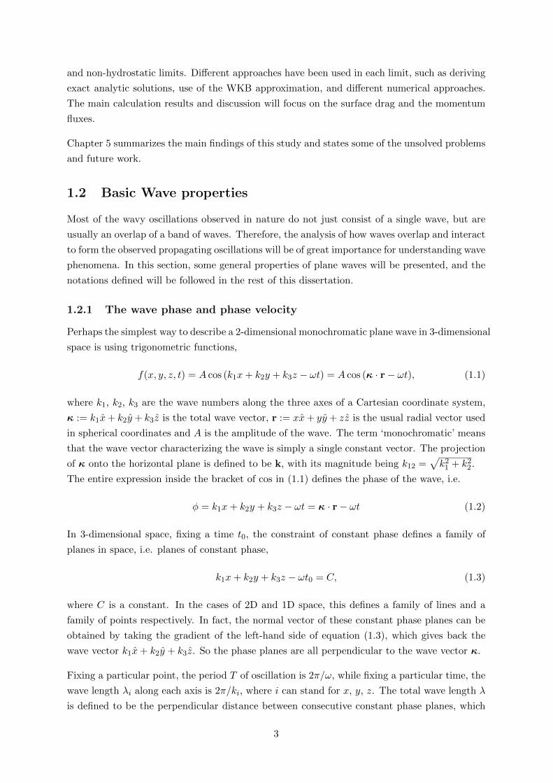
For simplicity, let us now consider a 2D case in the x-z plane. Fixing a particular position
(x0, z0) at time t = 0, the phase of the wave associated with this point is φ0 = kx0 + mz0.
The wave vector, lines of constant phase and total wave length are illustrated in figure (1.1(a)).
As time t evolves, the lines with constant phase evolve continuously. The velocity of motion of
these lines defines the phase velocity, which is given by the total wave length divided by the
period of oscillation, and its direction is along the wave vector,
vp =λ
T=
ω
|κ|. (1.5)
The projections of the phase line velocities onto the two axes give the phase velocity vpi along
each axis i, and they are related to the total phase velocity via the following equation,(1
vp
)2
=
(1
vpx
)2
+
(1
vpz
)2
, (1.6)
which in fact can be derived by using equation (1.4).
𝜆!
𝜆!
𝜆
𝑥
𝑧
(a)
Some Wave Mechanics 15
FIGURE 1.13 A ring wave on the surface of a calm pond moves with group velocity ug , butthe wavelets move with their individual phase speeds, c, which is a function of their wavenumbers,i.e., kN , kN−1, kN−1, . . . .
of the wave energy is considered that the problem becomes realistic. Indeed, it isthe energy transport that creates the wave. The wave does not create the energytransport. The speed and direction of energy transport is determined by the groupvelocity.
Following Lighthill (1978), imagine a stone thrown into a pond of still water.After the initial splash, we see a ring of water, a “ring wave,” moving away fromits center. If we could follow the wave and examine it closely, we would see thatthe surface of the wave is continually disturbed by a series of smaller waves orwavelets which propagate from the rear to the front of the larger wave. Thesewavelets were created when the stone struck the water surface. The energy of thatinitial disturbance was distributed over a wavenumber spectrum of waves. Thewavelets at the rear will have shorter wavelengths than the ones at the front, asillustrated in Fig. 1.13. These wavelets act to manifest the larger wave, which ineffect is a bundle or packet of waves referred to as a wave packet. Each wavelet ismoving at phase c(k), which is a function of its wavenumber k. The wavelets at thefront have larger wavelengths than the waves at the rear and, therefore have greaterphase speeds. However, it is clear that the wavelets are moving faster than wavepacket which we observe to have speed ug . The wavelets appear neither aheadnor behind the wave packet, and we conclude that they have no energy content. Ifthey did, then we would be able to observe them as they moved ahead of the wavepacket. Thus, the energy of the disturbance is contained in the wave packet whichwe can observe on the water’s surface. But what is the speed of this packet?
To analyze this energy transport let us consider the simplest case: a wave packetcomposed of only two waves traveling in the positive x-direction. Let the waveshave equal amplitudes, a, but slightly different frequencies, i.e., ω + δω, ω − δω,and wavenumbers, i.e., k + δk and k − δk. The superposition of these waves isgiven by
ζ = a cos[(k + δk)x − (ω + δω)t] + a cos[(k − δk)x − (ω − δω)t] . (1.21)
With some trigonometry, (1.21) can be written as
ζ = 2a cos(δkx − δωt) cos(kx − ωt) . (1.22)
(b)
Figure 1.1: (a) A schematic diagram showing a wave with wave vector κ. The red lines indicate lines
of constant phase. Note that λx and λz are both longer than λ, and they satisfy the relation of equation
(1.4). (b) A schematic diagram showing a cross-section of a ring-wave on water. N small oscillations
are superposed on at the surface of the ring-wave, each with a different phase speed c(kj), j = 1, 2, 3, ...
, N. The velocity of the main ring-wave is given by ug, which is in fact the group velocity of the wave.
(Source: Nappo (2012))
4

1.2.2 The group velocity and the dispersion relation
In fact, the phase of a wave simply represents a pattern of the oscillation. So, the phase velocity
refers to the movement of this pattern, but not to the movement of physical quantities. A more
interesting problem would be to understand how fast waves transport energy and momentum.
Indeed, wave energy and momentum must be carried with the group velocity of the wave, i.e.
the velocity of motion of the wave packets.
Usually, oscillations occur as a result of overlapping of waves with a band of wave numbers (or
wave vectors). In 1978, Lighthill observed that as a stone falls into a tank of water, a circular
ring-wave is generated in the water, which expands in the radial direction and spreads outward
(Nappo 2012). Moreover, as the circular ring-wave moves, small oscillatory phases are observed
on its surface, which appear to move at a different velocity relative to the ring. The ring-wave,
indeed, consists of waves with a continuous band of wave numbers, which have different phase
speeds on the water surface and hence cause the observed relative motion. However, those
small phases only appear on the surface of the ring-wave, but as they leave it, their amplitude
becomes zero. If the phase of a wave really carried energy, then the small phases should be sus-
tained without being destroyed. Therefore, the fact is that those small phases have no energy
content, while the energy is carried by the ring-wave. In fact, the appearance of the moving
ring-wave is due to the outward propagating energy, which allows the oscillations to appear and
take the shape of a water ring. Therefore, the velocity of the moving wave packet is defined to
be the group velocity.
The mathematical formulation of the group velocity will just be presented here without deriva-
tion. In general, for a 3D case, the oscillation frequency ω can be expressed as a function of
wave numbers ki, i = 1, 2, 3. The group velocity vg = (vgx, vgy, vgz) can be written as
vgx =∂ω
∂k1, vgy =
∂ω
∂k2, vgz =
∂ω
∂k3. (1.7)
The relation between ω and the wave numbers is called the dispersion relation. The dispersion
relation is of great importance since it describes how the phase and energy propagate in the
medium. For a special case in 1D space, if the phase speed of waves is independent of their wave
number, we have vp = ω/k = C, where C is constant, which means that the dispersion relation
is ω = C k. It can be seen easily that the group velocity and phase velocity are the same and
both independent of wave number. Such wave is described as non-dispersive. However, usually
waves are dispersive, such as the water ring discussed in the previous example. Each small wave
has its own phase speed c(kj) depending on its wave number kj , as shown in figure (1.1(b)).
Hence, different wave components will eventually spread away and change the initial wave form
as the wave propagates.
5

1.3 Linear Theory
The motions of the atmosphere under the assumption of inviscid adiabatic flow are governed
by the complicated primitive equations set (1.8), which contains 5 non-linear differential equa-
tions. Despite the fact that the primitive equations can capture many different phenomena of
the atmosphere, they contain more formation than necessary, including unimportant wave phe-
nomena such as sound waves, which do not have any meteorological significance. Such ‘noise’
embedded in the initial condition would cause numerical instability in meteorological models
(Lin 2007). Therefore, appropriate simplifications to the primitive equations are necessary for
studying the dynamics of the atmosphere. In this section, the result after those approximations
will be stated, but the derivation will not be presented. Interested readers may consult any
standard text books on atmospheric fluid dynamics.
Du
Dt− fv = −1
ρ
∂p
∂x(1.8a)
Dv
Dt+ fu = −1
ρ
∂p
∂y(1.8b)
Dw
Dt= −1
ρ
∂p
∂z− g (1.8c)
Dρ
Dt= −ρ(
∂u
∂x+∂v
∂y+∂w
∂z) (1.8d)
Dθ
Dt= 0, (1.8e)
where D/Dt = ∂/∂t+u∂/∂x+ v∂/∂y+w∂/∂z is the Lagrangian rate of change, u = (u, v, w)
is the total velocity, f is the Coriolis parameter, ρ is density of air, p is pressure, g is the
gravitational acceleration and θ is potential temperature. Note that the above equation set is
not closed. Closure of this equation set requires extra equations such as the equation of state
for ideal gas
p = ρRdT,
and the Poisson equation
θ = T
(psp
)Rd/cp,
where cp is the heat capacity of dry air under constant pressure, Rd is the ideal gas constant
for dry air, and ps is a reference pressure value, usually set to be 1000hPa.
1.3.1 The Boussinesq approximation and Linearization
The two main challenges of solving the primitive equations are those embedded small-scale wave
phenomena and the intrinsic non-linearity of these equations. Small-scale waves such as sound
waves can be filtered by the anelastic approximation and the Boussinesq approximation, which
may also be used to simplify the equations. It is first assumed that the density ρ and pressure
6

p can be written as
ρ(x, y, z, t) = ρr(z) + ρ′(x, y, z, t), (1.9a)
p(x, y, z, t) = pr(z) + p′(x, y, z, t) (1.9b)
and that the magnitude of perturbations ρ′ and p′ is much smaller than that of those reference
states ρr and pr. Then, in the subsequent simplifications, we may neglect the effect of ρ′ in
all equations, except the vertical momentum equation (Booker and Bretherton 1967). This
is because the atmosphere supports small-scale waves mainly via two mechanisms: one is the
compression force, and another is the buoyancy force (Lin (2007); Nappo (2012)). The com-
pression force arises from the compressibility of air, which produces acoustic waves with short
wave length, such as sound waves. Such short waves are regarded as ‘noise’ in the investigation
of atmospheric dynamics. The buoyancy force is due to the contrast of density between an
air parcel and its environment. Such buoyancy force causes oscillations of the air parcel and
produces gravity waves. Therefore, to focus on gravity waves it is necessary to kill off the com-
pression force by assuming no density variation in the continuity equation, but at the same time
allowing the density contrast in the vertical direction. Together with the hydrostatic balance,
the results of the Bousinesq approximation after simplification are expressed as,
Du
Dt− fv = − ∂
∂x
(∂p′
ρr
)(1.10a)
Dv
Dt+ fu = − ∂
∂y
(∂p′
ρr
)(1.10b)
Dw
Dt= − 1
ρr
∂p′
∂z− ρ′
ρrg (1.10c)
∂u
∂x+∂v
∂y+∂w
∂z= 0 (1.10d)
Dθ
Dt= 0, (1.10e)
The problem of non-linearity can be solved by the so-called linearization process, which assumes
that other field variables can also be written as their spatial mean plus a small variation.
u = (U(z), V (z), 0) + u′(t, x, y, z) (1.11a)
θ = θ(z) + θ′(t, x, y, z), (1.11b)
where the bar or capital letters denote time-averaged mean values and are assumed to only
vary in the z-direction if non-zero. A prime denotes both time- and spatially-dependent pertur-
bations. Note that the vertical velocity w is assumed to be a perturbation, since its average is
zero. Substitute (1.11) into (1.10) and simplify by assuming that any product of perturbations
7

is negligible, and then the final result is
∂u′
∂t+ U
∂u′
∂x+ V
∂u′
∂y+ w′
∂U
∂z− fv = − ∂
∂x
(∂p′
ρr
)(1.12a)
∂v′
∂t+ U
∂v′
∂x+ V
∂v′
∂y+ w′
∂V
∂z+ fu = − ∂
∂y
(∂p′
ρr
)(1.12b)
∂w′
∂t+ U
∂w′
∂x+ V
∂w′
∂y= − 1
ρr
∂p′
∂z+θ′
θg (1.12c)
∂u′
∂x+∂v′
∂y+∂w′
∂z= 0 (1.12d)
∂θ′
∂t+ U
∂θ′
∂x+ V
∂θ′
∂y+ w′
∂θ
∂z= 0, (1.12e)
1.3.2 The Taylor-Goldstein equation
We are now at the right point to derive the Taylor-Goldstein equation, which is the main target
we aim to solve in this study. Note that equation (1.12) includes the effect of rotation of the
Earth, which affects only large-scale motions. However, the scale of gravity waves that we are
interested in is small, so the Coriolis terms do not play an important role, and can be neglected.
Together with this assumption, we take the Fourier transform (see appendix B for the definition
of the pair of Fourier integrals) of equation (1.12) about its x, y and t dimensions, which is
equivalent to assuming that all the perturbation variables are of the form q′ = q(z)ei(k1x+k2y−ωt),
−iωu+ iUk1u+ iV k2u+dU
dzw = −ik1
ρrp (1.13a)
−iωv + iUk1v + iV k2v +dv
dzw = −ik2
ρrp (1.13b)
−iωw + iUk1w + iV k2w = − 1
ρr
dp
dz+θ
θg (1.13c)
ik1u+ ik2v +dw
dz= 0 (1.13d)
−iωθ + iUk1θ + iV k2θ +dθ
dzw = 0, (1.13e)
For simplicity, we assume the mean density ρr is constant. Then, it is possible to express all
other quantities in terms of w only. This yields the Taylor-Goldstein equation
d2w
dz2+
(N2κ2
Ω2+U ′′k1 + V ′′k2
Ω− (k21 + k22)
)w = 0, (1.14)
where Ω = ω −U · k is the so-called ‘Doppler-shifted intrinsic frequency’ of the wave, which
is in fact the frequency of the wave measured in the frame of reference of the mean wind (Lin
(2007); Nappo (2012)). The above equation is important because it contains only one unknown
variable w, and relations of w with all other quantities are known from equation (1.13). In
other words, equation (1.14) together with equation (1.13) is sufficient to determine the motion
of the atmosphere under the assumptions of linear theory. The remaining chapters will focus
8
on solving equation (1.14) subject to various situations such as different mountain width and
wind profiles.
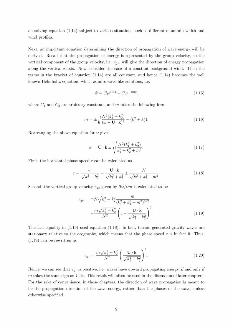
Next, an important equation determining the direction of propagation of wave energy will be
derived. Recall that the propagation of energy is represented by the group velocity, so the
vertical component of the group velocity, i.e. vgz, will give the direction of energy propagation
along the vertical z-axis. Now, consider the case of a constant background wind. Then the
terms in the bracket of equation (1.14) are all constant, and hence (1.14) becomes the well
known Helmholtz equation, which admits wave-like solutions, i.e.
w = C1eimz + C2e
−imz, (1.15)
where C1 and C2 are arbitrary constants, and m takes the following form
m = ±
√N2(k21 + k22)
(ω −U · k)2− (k21 + k22). (1.16)
Rearranging the above equation for ω gives
ω = U · k±
√N2(k21 + k22)
k21 + k22 +m2. (1.17)
First, the horizontal phase speed c can be calculated as
c =ω√
k21 + k22=
U · k√k21 + k22
± N√k21 + k22 +m2
. (1.18)
Second, the vertical group velocity vgz given by ∂ω/∂m is calculated to be
vgz = ∓N√k21 + k22
m
(k21 + k22 +m2)3/2
= −m√k21 + k22N2
(c− U · k√
k21 + k22
)3
. (1.19)
The last equality in (1.19) used equation (1.18). In fact, terrain-generated gravity waves are
stationary relative to the orography, which means that the phase speed c is in fact 0. Thus,
(1.19) can be rewritten as
vgz =m√k21 + k22N2
(U · k√k21 + k22
)3
. (1.20)
Hence, we can see that vgz is positive, i.e. waves have upward propagating energy, if and only if
m takes the same sign as U ·k. This result will often be used in the discussion of later chapters.
For the sake of convenience, in those chapters, the direction of wave propagation is meant to
be the propagation direction of the wave energy, rather than the phases of the wave, unless
otherwise specified.
9

Chapter 2
Flow over a 2-D isolated mountain
In this chapter, we are going to investigate mathematically the formulation of terrain gen-
erated gravity waves and some relevant physical quantities, by illustrating an example of a
two-dimensional mountain ridge with a constant basic wind profile. Terrain generated gravity
waves affect the atmospheric circulation by transporting energy and momentum of the mean
flow from the lower atmosphere to the upper atmosphere and hence contribute to modify the
global circulation (McFarlane 1987). Several important quantities, such as the surface drag,
wave momentum flux, and the critical level will be formulated mathematically to facilitate the
discussion in later chapters, which will extend the investigation to 3-dimensional space.
As will be shown in the 2-D example, the flow may exhibit different behaviors for different
horizontal wave numbers k. In the case where the atmosphere is well stratified and the moun-
tain is broad and gentle, gravity waves can be supported by the buoyancy force and are capable
to propagate vertically in the atmosphere. However, if the atmosphere is weakly stratified, or
with strong basic wind, gravity waves may not be able to propagate vertically and have to be
decaying throughout the atmosphere (Nappo 2012). Such different types of flow can be clas-
sified into different regimes of the wave solution. The exploration of different solution regimes
enable us to distinguish the criteria supporting the propagation of gravity waves.
2.1 Mountain profile
In this section, we consider a bell-shaped mountain (or the so called Witch of Agnesi mountain
profile),
h(x) =hma
2
x2 + a2(2.1)
where hm is the mountain height and a is the horizontal scale of the mountain. This mountain
form had been widely used in many published books and papers (Lin (2007); Nappo (2012) and
10

Teixeira and Miranda (2009)), because of the simple form of its Fourier transform,
h(k) =hma
2e−|k|a, (2.2)
which will greatly facilitate the calculation of the wave solution. It turns out that the Fourier
transform of the orography profile plays an important role in the process of generating gravity
waves (Lin 2007). By Fourier analysis, we know that a periodic function on a real axis takes a
discrete wave spectrum, i.e. the constituent wave numbers are discrete. However, if the function
is not periodic, such as an isolated mountain profile in this case, the function is then composited
of a continuous band of wave numbers k (Nappo 2012). Hence, the steady state Taylor-Goldstein
equation has to be solved for each of these wave numbers in order to compute those relevant
quantities, such as the pressure perturbation, surface drag and vertical momentum fluxes, etc.
Figure (2.1(a)(b)) shows the distribution of the bell-shaped mountain and the product of k and
h(k). The importance of the function kh(k) will be discussed in the coming section.
!40 !20 0 20 40
0.2
0.4
0.6
0.8
1.0
1.2
(a) h(x)
0.1 0.2 0.3 0.4 0.5
0.05
0.10
0.15
(b) kh(k)
Figure 2.1: (a) shows an isolated bell-shaped mountain located at the origin, with mountain
height hm equal 1 unit (or equivalently the scale is normalized by the height of the mountain),
while its scale width is a = 10 hm. (b) shows the distribution of kh(k), which has its maximum
at the wave number 1/a = 0.1.
2.2 Different regimes of solution
In chapter 1, by taking the Fourier transform of equation (1.12), we have derived the Taylor-
Goldstein equation. In this subsection, a detailed solving process of equation (1.14) for w(k),
which is the Fourier transform of the vertical velocity perturbation w′, will be presented. The
procedure follows the idea in the book by Lin (2007).
Consider now the 2D steady-state form of the Taylor-Goldstein equation (1.14):
w′′(z) + (l(z)2 − k2)w(z) = 0 (2.3)
11

where the function l(z) is the Scorer parameter
l2(z) =N2
U(z)2− U ′′(z)
U(z). (2.4)
The lower boundary condition for the total velocity u = (U(z) + u′(x, z), w′(x, z)) is the ‘no-
normal-flow’ boundary condition, which, after linearization, requires that
U(z = 0)dh(x)
dx− w′(x, 0) = 0. (2.5)
By taking the Fourier transform of (2.5), we have
w(0) = ikU(0)h(k). (2.6)
If we assume the Scorer parameter l is constant w.r.t z, e.g. a constant background wind profile
U and static stability N , then equation (2.3) becomes the famous Helmholtz equation, which
exhibits wave-like solutions. In fact, equation (2.3) has solution of the following form
w(z) = w(0)ei√l2−k2z if l2 > k2 and (2.7a)
w(z) = w(0)e−√k2−l2z if l2 < k2. (2.7b)
By the above equations, the wave solution exhibits different behaviors in the two cases l2 > k2
and k2 > l2. For the first case (l2 > k2), oscillatory waves can be observed, while for the latter
case (l2 < k2), the wave becomes evanescent, i.e. the wave amplitude is exponentially decaying.
A nice explanation described in the book by Nappo (2012) is helpful to see the physical picture
in these two cases. Suppose now that k is fixed and neglect for the moment the second term
in equation (2.4). Then l2/k2 can be written as N2
U2k2= N2
1/t2adv, where tadv is the time for the
flow to complete one single oscillation by the means of advection. Thus, the criteria that an
oscillatory wave can only exist when l2/k2 > 1 implies that the advection time tadv of this
wave has to be larger than the period of oscillation at the natural oscillation frequency N , i.e.
we have to allow enough time for the air parcel to oscillate by the means of buoyancy. If this
criterion cannot be met, then the wave oscillation cannot be completed, and hence the wave
amplitude must be decaying. This leads to the appearance of evanescent waves.
Recall that an isolated mountain profile is composited of a continuous band of wave num-
bers k, so we have to consider all these wave numbers in order to solve for w′(x, z). With the
two simple analytic members of the solution basis in equation (2.7), the solution for w′(z) can
be found easily by performing an inverse Fourier transform back to physical space, which yields
w′(x, z) = 2Re
[∫ l
0iU kh(k)ei
√l2−k2zeikxdk +
∫ ∞l
iU kh(k)e−√k2−l2zeikxdk
]. (2.8)
The above integral is split into two parts according to the different expressions in (2.7). The
real part taken in equation (2.8) is due to the symmetry property of the integral, and also
because w′(x, z) is a real quantity.
12
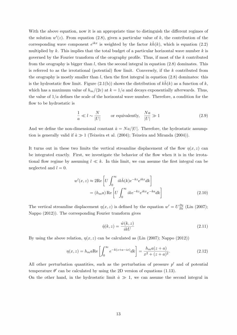
With the above equation, now it is an appropriate time to distinguish the different regimes of
the solution w′(z). From equation (2.8), given a particular value of k, the contribution of the
corresponding wave component eikx is weighted by the factor kh(k), which is equation (2.2)
multiplied by k. This implies that the total budget of a particular horizontal wave number k is
governed by the Fourier transform of the orography profile. Thus, if most of the k contributed
from the orography is bigger than l, then the second integral in equation (2.8) dominates. This
is referred to as the irrotational (potential) flow limit. Conversely, if the k contributed from
the orography is mostly smaller than l, then the first integral in equation (2.8) dominates: this
is the hydrostatic flow limit. Figure (2.1(b)) shows the distribution of kh(k) as a function of k,
which has a maximum value of hm/(2e) at k = 1/a and decays exponentially afterwards. Thus,
the value of 1/a defines the scale of the horizontal wave number. Therefore, a condition for the
flow to be hydrostatic is
1
a l ∼ N
|U |or equivalently,
Na
|U | 1 (2.9)
And we define the non-dimensional constant a = Na/|U |. Therefore, the hydrostatic assump-
tion is generally valid if a 1 (Teixeira et al. (2004); Teixeira and Miranda (2004)).
It turns out in these two limits the vertical streamline displacement of the flow η(x, z) can
be integrated exactly. First, we investigate the behavior of the flow when it is in the irrota-
tional flow regime by assuming l k. In this limit, we can assume the first integral can be
neglected and l = 0.
w′(x, z) ≈ 2Re
[U
∫ ∞0
ikh(k)e−kzeikxdk
]= (hma) Re
[U
∫ ∞0
ike−kzeikxe−kadk
](2.10)
The vertical streamline displacement η(x, z) is defined by the equation w′ = U ∂η∂x (Lin (2007);
Nappo (2012)). The corresponding Fourier transform gives
η(k, z) =w(k, z)
ikU(2.11)
By using the above relation, η(x, z) can be calculated as (Lin (2007); Nappo (2012))
η(x, z) = hmaRe
[∫ ∞0
e−k(z+a−ix)dk
]=
hma(z + a)
x2 + (z + a)2. (2.12)
All other perturbation quantities, such as the perturbation of pressure p′ and of potential
temperature θ′ can be calculated by using the 2D version of equations (1.13).
On the other hand, in the hydrostatic limit a 1, we can assume the second integral in
13

equation (2.8) can be neglected. Thus, w′(x, z) and η(x, z) can be integrated as
w′(x, z) ≈ 2Re
[U
∫ ∞0
ik
(hma
2
)e−kaeilzeikxdk
](2.13)
η(x, z) ≈ hmaRe
[∫ ∞0
eilze−k(a−ix)dk
]=hma cos lz − x sin lz
x2 + (z + a)2. (2.14)
Figure(2.2) shows the flow trajectories and pressure perturbation under different regimes.
2.3 The surface drag and momentum fluxes: conceptually
Figure 2.2 shows the streamlines η(x, z) and the pressure perturbation p′(x, z) in the differ-
ent flow regimes described in the previous section. As shown in figure (2.2(a)), a important
difference between the irrotational flow and the other two types of flow is that the pressure
distribution of irrotational flow is symmetric on both upstream and downstream sides of the
mountain, while the pressure distribution is mostly asymmetric in the hydrostatic limit. It
turns out that this asymmetric distribution of pressure plays a crucial role in the generation of
the surface drag force and wave momentum fluxes.
The formation of the drag force can be understood by using some basic mechanics (Teixeira
et al. (2004); Teixeira and Miranda (2004); Nappo (2012)). The uneven distribution of pressure
on two sides of the mountain contributes to a pressure-gradient force exerted to the obstacle
by the flow (Lin (2007); Teixeira et al. (2004)). Then the famous Newton’s third law of motion
states that,
For any force exerted by an object A on an object B, there is a reaction force
exerted by object B on object A at the same time, with the same magnitude
but opposite direction.
Therefore, the existence of a surface pressure gradient force on the mountain means that there
is a reaction drag force exerted on the flow by the mountain. This drag force creates flow
perturbation patterns which carry mean flow horizontal momentum and propagate upwards
(Nappo 2012). The stronger the drag force the flow experiences, the greater the upward propa-
gating momentum flux is. As a result, the drag force represents the total amount of horizontal
momentum being able to be transported vertically to the upper atmosphere in the form of
gravity waves (Teixeira and Miranda 2009). As we can see from figure(2.2(a)), gravity waves
do not appear (the flow amplitude decays exponentially with height) in the case of irrotational
potential flow due to the absence of the pressure difference on the two sides of the mountain
(and hence the drag force). For the other two types of flow, wavy patterns of the streamlines
and pressure can be clearly observed in the vertical direction. Associated with them are strong
surface pressure gradients and surface drag forces, which are consistent with the above analysis.
These can be verified easily in figure 2.2(b) and 2.2(c).
14

−10 −8 −6 −4 −2 0 2 4 6 8 100
1
2
3
4
5
6
7
8
−7
−6
−5
−4
−3
−2
−1
0
x 10−3
(a) Irrotational flow: a = hm = 1km, N = 0.01, U = 100ms−1
−15 −10 −5 0 5 10 150
1
2
3
4
5
6
7
8
9
−5
−4
−3
−2
−1
0
1
2
3
4
x 10−5
(b) Intermediate: a = hm = 1km, N = 0.01, U = 10ms−1
−40 −20 0 20 40 600
1
2
3
4
5
6
7
8
9
−8
−6
−4
−2
0
2
4
6
8
x 10−5
(c) Hydrostatic flow: a = 10km, hm = 1km, N = 0.01, U = 10ms−1
Figure 2.2: (a) shows a contour plot of the pressure perturbation (colored lines), and trajectories
of the flow (black lines) in the irrotational potential flow. The flow is evanescent above the
mountain. (b)(c) show filled contour plots of the pressure perturbation and trajectories of the
flow (white lines) in the intermediate and hydrostatic regimes, respectively. The mountain
profiles are depicted by brown dashed lines. Both the x-and y- axes are scaled by the height of
mountain hm. It is clear that the wave pattern is vertically aligned in hydrostatic limit, while
the wave pattern tilts downstream of the mountain in the intermediate limit.
15

Mathematically, since the quantity l is actually the total wave number, while k is the
horizontal wave number, the assumption that l k implies immediately that the total wave
vector is almost vertically orientated. Moreover, the stationary nature of the mountain wave
can be explained by the fact that the existence of a drag force arises from the surface orography,
so the gravity wave patterns have to remain attached to the orography (which is their source).
2.4 The surface drag and momentum fluxes: mathematically
With the conceptual discussion of the surface drag and momentum fluxes in the previous section,
in this section the mathematical formulation of these quantities will be illustrated. The approach
follows books by Lin (2007) and Nappo (2012).
Recall that the surface drag D is created due to the net pressure gradient force resulting from
the asymmetric pressure distribution on the orographic profile. One equation directly related
with the pressure gradient force is the horizontal momentum equation, i.e. the 2D version of
equation (1.12a)
U∂u
∂x+ w′
∂U
∂z+
1
ρr
∂p′
∂x= 0 (2.15)
For an isolated mountain profile, h(x) → 0 as z → ±∞. So we multiply equation (2.15) at
z = 0 by h(x) and integrate over the entire x-axis.∫ +∞
−∞h(x)U
∂u′
∂xdx+
∫ +∞
−∞h(x)w′
dU
dzdx+
∫ +∞
−∞h(x)
1
ρr
∂p′
∂xdx = 0 (2.16)
By using integration by parts, the first integral I1 can be evaluated as
I1 = −∫ +∞
−∞Uu′
dh
dxdx = −
∫ +∞
−∞u′w′(0)dx (2.17)
The last equality has used equation (2.5). Moreover, also by using equation (2.5), the second
integral I2 vanish.
I2 =
∫ +∞
−∞h(x)w′
dU
dzdx = U
dU
dz
∫ +∞
−∞h(x)
dh
dxdx
= UdU
dz
∫ +∞
−∞
1
2
dh2
dxdx
= 0 (2.18)
The same approach is applied to the integral I3
I3 =
∫ +∞
−∞h(x)
1
ρr
∂p′
∂xdx = −
∫ +∞
−∞
p′
ρr
dh
dxdx (2.19)
Adding the three integrals, equation (2.16) can be rewritten as
−ρr∫ +∞
−∞u′w′(0)dx =
∫ +∞
−∞p′dh
dxdx (2.20)
16

In the above equation (2.20), the R.H.S is the integral of the product of the pressure and the
elevation gradient, which is the net pressure gradient force experienced by the orography; while
the L.H.S is the integral of the product of the horizontal momentum and vertical velocity, which
is the stress force experienced by the mean flow. Therefore, we can see that equation(2.20) is
in fact a statement of Newton’s third law, as explained in the previous section.
Thus, the formal surface drag force (at z = 0) is defined as
D = −∫ ∞−∞
ρru′w′dx =
∫ ∞−∞
p′dh
dxdx, (2.21)
which is actually equation (2.20).
Equation (2.20) defines the surface drag in terms of the pressure gradient force at the surface.
Despite the fact that the R.H.S loses its meaning above the surface, the quantity on the left
hand side the L.H.S does not. However, this limitation can be avoided by replacing h by η,
i.e. the vertical streamline displacement of the flow. Moreover, the product of ρru′ and w′
has the physical meaning of vertical advection of horizontal momentum. Thus, integrating this
quantity over the entire real axis at any level describes the momentum flux at that level. Thus
the momentum flux can be formulated as
M = −∫ ∞−∞
ρru′w′dx (2.22)
From this definition we can see immediately that the momentum flux at the surface gives exactly
the surface drag. In other words, this again demonstrates that the drag force gives the total
amount the horizontal momentum flux that can be produced by the flow over the orography
(Teixeira and Miranda 2009).
2.5 Height dependent Scorer Parameter
In the previous sections, we only focused on the situation when both the basic wind profile U(z)
and the Brunt-Vaisala frequency N are constant with respect to height, i.e. a constant Scorer
parameter. However, reality is not always that simple. The basic wind profile can be easily
altered by a lot of factors, such as variations of the surface temperature, or orographic distri-
bution. In this situation, the Taylor-Goldstein equation (2.3) cannot be solved analytically in
general for arbitrary wind profiles. Hence, numerical calculations are necessary for investigating
the behavior of the atmospheric motions (Grisogono (1994); Shutts (1995); Shutts and Gadian
(1999)).
Despite this difficulty, the behavior can still be analyzed using reasonable simplifications and
assumptions. A common approach is to assume that the variations of the Scorer parameter
(2.4) in the vertical direction are slow. Recall that when the Scorer parameter l is constant with
17

height, equation (2.3) admits wave solutions (2.7), in which the wave number is m =√l2 − k2.
If now the Scorer parameter is slowly-varying, this means that m is slowly varying as well.
Therefore, it is reasonable to assume that the solution is still oscillatory in sinusoidal form,
thus the solution is approximated as
w(k, z) ≈ A(k, z) exp(iφ(k, z)), (2.23)
where A(k, z) is the height dependent amplitude and φ(k, z) is the height dependent phase
for the wave solution. In fact, the above idea gives the motivation for the WKB (Wentzel,
Kramers, Brillouin) method, which has been used and discussed in a wide range of papers
(Shutts (1995); Teixeira and Miranda (2004); Teixeira and Miranda (2006)). The discussion of
the WKB approximation will be continued in chapter 3, in which this method will be applied
to two different wind profiles, and its validity will be analyzed and compared with numerical
calculations.
2.5.1 The critical level
In the previous example of gravity wave behavior over 2-D orography, we aimed at solving the
Taylor-Goldstein equation (2.3). One may note that the Scorer parameter (2.4) may suffer
from singularities if the denominator U(z) (in the 3D case is U · k instead) becomes zero at
some level zc. This level zc is defined to be the critical level. By the second-order nature of the
Taylor-Goldstein equation, the first order derivative of the solution w(z) is no longer continuous
at critical levels.
The study of critical levels began early in the 1960s. At that time meteorologists mainly
focused on critical levels occuring in a sheared 2D flow over an isolated mountain ridge. Many
studies (Bretherton (1966); Booker and Bretherton (1967); Breeding (1971)) showed that the
wave energy would be absorbed and wave magnitude would be attenuated by a factor of
exp(π√Ri− 0.25) (definition for Ri is in appendix A) as the waves approach and cross the
critical level. A more physical picture of this effect is that any wave packet will not reach
the critical level in any finite amount of time and its vertical group velocity wg approaches 0
as it moves towards the critical level (Bretherton 1966). The mathematical derivation of the
asymptotic behavior of gravity waves near a critical level is provided in appendix A, and the
over-all result is expressed by equation (A.24),
w(z) =√
(z − zc)(C↑ei(sgn) ln (z−zc)µ + C↓e−i(sgn) ln (z−zc)µ
)for z > zc
w(z) = −i(sgn)√
(zc − z)(C↑eπµei(sgn) ln (zc−z)µ + C↓e−πµe−i(sgn) ln (zc−z)µ
)for z < zc
where the terms with coefficient C↑ represent waves with upward propagating energy, while
terms with coefficient C↓ represent waves with downward propagating energy. The behavior
across the critical level is shown in figure (2.3).
It is important to note that there is a difference in the meaning of critical levels between
18

2-D and 3-D cases. In a 2-D situation, a critical level appears only when the basic wind U(z)
is zero at some height zc, while in the 3-D case, it refers to the levels where the vector U is
perpendicular to the horizontal wave vector number k. In fact, the definition of a critical level in
the 3-D case is more general, in the sense that the 2-D definition can be viewed as a restriction
by reduction of dimensions. Following this point of view, it should be noted that the critical
level in a 2-D situation is k-independent since the horizontal dimension contains only the x
direction, so the dot product U · k can be zero if and only if U(z) = 0. But in a 3D situation,
the critical level zc is k-dependent, except when U(z) = 0. Thus, Broad (1995) designates the
critical level zc at which U(z) = 0 as a ‘total critical levels’ in the 3-D situation. Moreover,
with 3D orography, at any height z, there is always some wave vector k perpendicular to the
basic wind U(z). This means that every level in the atmosphere is the critical level for a certain
wave vector k. So this contributes to the so-called ‘critical layer’, as opposed to discrete critical
levels. Moreover, the k-dependent property of the critical levels contributes to a directional
filtering effect of critical layers (Broad (1995); Shutts (1995)). In chapter 3, a more detailed
discussion about the effect of critical levels in a 3-D situation will be presented.
2000 4000 6000 8000 10000 12000 14000 16000
−0.25
−0.2
−0.15
−0.1
−0.05
0
0.05
0.1
0.15
0.2
0.25
Real part of w(z)Imagary part of w(z)
Figure 2.3: shows the behavior of the real (blue) and imaginary (green) parts of w(z) around
a critical level zc for a particular wave vector k in a 3D situation. The wave becomes highly
oscillatory as it approaches zc (in fact its frequency approaches infinity), and the amplitude of
the wave shows a shape drop (by a factor of e−πµ, with µ = 1.4234 and Ri = 2.276 in this
figure) once it passes through zc. Both the units for the x and y-axis in this figure are arbitrary.
19

Chapter 3
Flow Over a 3-D Isolated Mountain
in the Hydrostatic Regime
In this chapter, we are going to investigate mountain waves generated by flow over a 3-D isolated
mountain in the hydrostatic limit. Two simple height-dependent wind profiles will be examined:
a linear wind profile with directional shear and a turning wind profile. Reasons for choosing
these wind profiles are that, first, they are simple and can be described easily by elementary
functions, and second, the directionality of the wind profile allows the existence of a critical
layer, i.e. a layer of the atmosphere in which any level is a critical level for a certain wave
vector k. Two methods, namely the WKB approximation and a numerical method developed
by Siversten (1972), will be adopted to solve the Taylor-Goldstein equation, and their results
will be presented and compared.
3.1 Setting of the problem
An inviscid, irrotational, steady flow can be captured by the steady-state version of the lin-
earized 3-D Boussinesq equations (1.12), which can be used to derive the steady-state Taylor-
Goldstein equation,
w′′(z) +
[N2k212
(Uk1 + V k2)2− U ′′k1 + V ′′k2
Uk1 + V k2− k212
]w(z) = 0, (3.1)
where k1 and k2 are wave vectors associated with x and y directions, and k12 :=√k21 + k22. In
the 3D case, the Scorer parameter l(z) is then defined by the following equation
l2(z) =N2k212
(Uk1 + V k2)2− U ′′k1 + V ′′k2
Uk1 + V k2(3.2)
Recall that in the hydrostatic limit, the magnitude k12 of the horizontal wave vectors k con-
tributing to the orographic profile is much smaller than that of the total wave number l, so that
the term −k212 in equation (3.1) can be neglected. Thus, equation (3.1) becomes
w′′(z) +
[N2k212
(Uk1 + V k2)2− U ′′k1 + V ′′k2
Uk1 + V k2
]w(z) = 0. (3.3)
20

If the static stability coefficient N is real and varies gently with height as well as U, then the
consequence of this assumption is that any wave being considered can freely propagate vertically
in the atmosphere, i.e. the associated solution of w(z) must be in the form of a propagating
wave at any level of the atmosphere. Therefore, wave reflection phenomenon does not occur.
With this observation, it is possible to include only waves with upward propagating energy.
The full atmospheric setting will be discussed next together with consideration of the critical
layer and the wind profile.
3.1.1 The critical layer
For flow over a 3-D isolated mountain, given a certain wave vector, the associated critical level is
defined as the altitude where the basic flow U is perpendicular to the horizontal wave vector k.
The effect of the critical level is that the wave energy and momentum is effectively attenuated
and absorbed by a factor of e−πµ into the mean wind without being reflected (Grubisic and
Smolarkiewicz 1997), as discussed in chapter 2. Therefore, if the direction of the basic wind
profile turns with height, then it induces a continuous region in the atmosphere, in which each
level is a critical level for a certain horizontal wave vector k (Shutts 1998). This region is
the critical layer, as explained in chapter 2. Thus, the existence of a directional shear will
be a necessary condition for the occurrence of such a layer. The effect of such a layer is well
summarized in the paper by Broad (1995), where it is shown
U(z) · dτ (z)
dz= 0, (3.4)
where τ (z) = (τx(z), τy(z), 0) is the wave stress vector, which is a generalized 3D version of the
wave stress defined inside the integral of equation (2.22).
Equation (3.4) states that the vertical gradient of the wave stress vector (and hence that of the
vertical momentum flux vector) must be perpendicular to the mean wind U(z). This means that
there is a filtering effect of vertical momentum flux occurring along the direction perpendicular
to the mean wind, which is the so-called ‘directional filtering effect’ of the critical layer. Such a
filtering effect throughout the critical layer is the interaction between the gravity waves and the
mean wind (i.e. the deposition of wave energy and momentum) (Miranda and James (1992);
Hines (1988); Shutts (1998)). For simplicity, we will only consider the situation where each
horizontal wave vector k can have at most one critical level in the atmosphere, which means
that the turning angle of the mean wind cannot exceed 180.
3.1.2 The wind profiles
As mentioned previously, two wind profiles will be examined in this chapter. The first one is a
linear wind profile with directional shear, which can be formulated as
Ulinear(z) = (U(z), V (z)) = (U0 − αz, U0), (3.5)
where α is the shear strength and U0 is the surface wind magnitude for each component. Since
Ulinear(0) at the surface has both x and y components equal to U0, this basic wind makes an
21

angle of π/4 relative to the x-axis at the surface, and this angle approaches π at infinity. But
due to computational limitations, the domain being considered must be finite, and hence the
wind can only turn by a certain angle θmax at the top of the domain zmax, as shown in fig-
ure (3.1(a)). Nevertheless, regardless of computational limitations, the atmosphere can still be
considered as an infinitely extended troposphere with a height-independent stability constantN .
The second wind profile being considered is the turning wind profile,
Uturning(z) = (U(z), V (z)) = (U0 cos (βz), U0 sin(βz)), (3.6)
where β is the rate of turning of the basic wind with respect to height and U0 is the wind
magnitude. As required, the wind can at most turn by an angle of π from 0 at the surface to
π at the top of the computational domain zmax, as shown in figure (3.1(b)).
(a) Linear wind profile (b) Turning wind profile
Figure 3.1: (a) shows a schematic diagram of the linear wind profile. (b) shows a schematic diagram
of the turning wind profile.
3.1.3 The mountain profile
Similar to the case of a 2-D isolated mountain, the mountain being considered in this chapter
is a 3-D circular bell-shaped mountain (i.e.Witch of Agnesi mountain profile),
h(x, y) =hm
(1 + (x/a)2 + (y/a)2)3/2(3.7)
where hm is the height of the mountain, and a is the width (both in the x and y directions).
The associated Fourier transform is
h(k1, k2) =hma
2
2πe−ak12 . (3.8)
As usual, two boundary conditions are required to solve the Taylor-Goldstein equation (3.3).
With the above choices for the atmospheric and orographic profiles, the linearized boundary
condition at the surface analogous to equation (2.5) is formulated as
w(z = 0) = ih [U(z = 0)k1 + V (z = 0)k2] for z = 0, (3.9)
22

which is the ‘no-normal-flow’ boundary condition. Another boundary condition is employed at
z → +∞, requiring that only waves with upward propagating energy are included. This is the
so-called radiation boundary condition. Its implementation will be discussed separately in each
of the methods being used.
3.2 Methodology
In this section, we are going to investigate two methods to solve equation (3.3). The first one
is a numerical method proposed by Siversten (1972), which has been adopted in Teixeira and
Miranda (2006) to investigate the effect of sheared flow over elliptical mountains. The other one
is a popular asymptotic method, the WKB (Wentzel-Kramers-Brillouin) approximation, which
has been briefly mentioned in chapter 2. The advantage of the WKB approximation is that it
provides an approximated analytic expression, which is helpful for the analysis and calculation
of some important quantities, such as the surface drag, momentum fluxes and their divergence
(Teixeira et al. (2004); Teixeira and Miranda (2009)).
However, before introducing the formulation of these two methods, it is worth noting that the
steady-state Taylor-Goldstein equation (3.1), in fact, admits an exact solution for the linear
wind profile (3.5) in both the hydrostatic and the non-hydrostatic limits. The hydrostatic exact
solution, which has been adopted by Teixeira et al. (2008), can be written in terms of simple
elementary functions, whilst the non-hydrostatic solution has to be expressed in terms of special
functions, more specifically Bessel functions. The details for the non-hydrostatic solution will
be discussed in chapter 4. With the aid of the exact solution for the linear wind profile in
the hydrostatic limit, the accuracy of the numerical method by Siversten (1972) can first be
demonstrated, so that it can be safely applied to calculate w for the turning wind profile.
3.2.1 Exact solution for linear wind profile in hydrostatic limit
By using equation (3.5), equation (3.3) can be simplified as
w′′(z) +
(N2k212
(U0(k1 + k2)− αk1z)2
)w(z) = 0. (3.10)
The general solution of the above equation is (Teixeira et al. 2008)
w(z) = C↑(
1− αk1z
U0(k1 + k2)
)1/2+i(sgn)µ
+ C↓(
1− αk1z
U0(k1 + k2)
)1/2−i(sgn)µ, (3.11)
where sgn = sign(−αk1) is the sign of the derivative of U · k at the critical level zc and µ =√N2k212/(αk1)
2 − 0.25. It will be shown in the following that the first term is associated with
upward propagating waves, whilst the second term represents downward propagating waves.
23

The corresponding vertical wave number m can be calculated as
m = −iw′
w
= (sgn)µ1
z − U0(k1+k2)αk1
− i
2
1
z − U0(k1+k2)αk1
. (3.12)
In fact, given a horizontal wave vector k = (k1, k2), the associated critical level for this linear
wind profile is U0(k1+k2)αk1
. Therefore, the real part of m is
Re(m) = (sgn)µ1
z − zc. (3.13)
If sgn > 0, then U ·k is positive above zc, and negative below zc. And 1/(z−zc) is also positive
above zc and negative below zc. Thus, Re(m) always takes the same sign as U · k. The same
result can be reached if sgn < 0. Thus, the first term is associated with upward propagating
waves, according to the conclusion in equation (1.20). Since in the hydrostatic limit, we are
only concerned about upward propagating waves, only the first term is relevant to the following
investigation.
3.2.2 A Linear numerical model
In this section, we are going to investigate a numerical method proposed by Siversten (1972),
and the discussion follows the idea of the paper by Teixeira and Miranda (2006). Solving
the 2nd-order Taylor-Goldstein equation as a boundary value problem requires two boundary
conditions. One of those is at the surface and assumes no normal flow. However, the radiation
boundary condition at the upper boundary is less trival to apply. This may pose challenges if
one attempts to solve the problem using methods such as finite differences or finite elements.
The advantages of the method by Siversten are that, first, it allows us to choose the desired
branch of the wave (in terms of direction of energy propagation), so that the radiation boundary
condition can be easily imposed. Second, it enables an accurate implementation of the lower
boundary condition by embedding this boundary condition in the solution form (Teixeira and
Miranda 2006).
Mathematical formulation
In general, the solution to (3.3) can be written in the following form
w(z) = w(0) exp
i
∫ z
0m(ζ)dζ
, (3.14)
where m is the vertical wave number. By substituting (3.14) into (3.3), then (3.3) is reduced
to a 1-st order non-linear differential equation for m (Teixeira and Miranda 2006).
im′ −m2 +N2k212
(Uk1 + V k2)2− U ′′k1 + V ′′k2
Uk1 + V k2= 0 (3.15)
24

The lower boundary condition is implicitly included in the solution form (3.14), so the boundary
condition for (3.15) must be consistent with the upper radiation boundary condition.
Boundary condition
In fact, the correct boundary condition for (3.15) depends on the existence of the critical level.
Fixing a particular wave number k, if a critical level does not exist, or it exists far away from the
calculation domain, then we may assume that m reaches a constant at the top of the calculation
domain, and the curvature of U is basically 0, so that m′ = 0 and the curvature term of (3.15)
can be dropped. Thus,
m(zmax) =Nk12
U(zmax)k1 + V (zmax)k2(3.16)
On the other hand, if a critical level appears within the domain or near the top of the domain,
then the asymptotic behavior of m must be used. From appendix A, we know that w becomes
highly oscillatory as z approaches zc, which means that m → ∞ as z → zc. However, infinity
is not a numerically favorable quantity, so a good way to tackle this problem is to solve for the
inverse of m. Define L = 1/m, then (3.15) can be converted into a differential equation for L
L′ = i
[1−
N2k212
(Uk1 + V k2)2− U ′′k1 + V ′′k2
Uk1 + V k2
L2
](3.17)
The dominant behavior of L near the zc can be obtained by using a Frobenius expansion,
following a similar approach to that in appendix A, we have
L±(z) =z − zc
− i2 ±
Nk12U ′(zc)k1+V ′(zc)k2
√1− 1
4(U ′(zc)k1+V ′(zc)k2)2
N2k212
= ±(U ′(zc)k1 + V ′(zc)k2)(z − zc)Nk12
√1− 1
4
(U ′(zc)k1 + V ′(zc)k2)2
N2k212
+ i(z − zc)(U ′(zc)k1 + V ′(zc)k2)
2
2N2k212for z near zc (3.18)
For a wave with upward propagating energy, we require that Re(m) takes the same sign as
Uk1 + V k2. This is true for L as well, since L = 1/m, so we require that the real part of L
takes the same sign as (U ′(zc)k1 + V ′(zc)k2)(z − zc). Thus, we see in (3.18) that the positive
branch L+ is associated with upward propagating energy. Therefore, (3.18) allows us to select
the correct branch of the wave solution to satisfy the radiation boundary condition.
With the positive branch L+ in equation (3.18), the behavior of m near the critical level is
determined, and m in other regions can be solved by either (3.15) or (3.17) using a numerical
method. The Runge-Kutta 4th-order method is adopted for this purpose.
25

Error analysis
Since this numerical method solves for the vertical wave number m, instead of w, the error
analysis will be based on the error associated with m. A wave vector k with its critical level zc
located near the surface is chosen. The integration of m is carried out above zc from a certain
grid point near zc to the top of the calculation domain. Exact value of m is used at the first
grid point near zc as the initial value for the numerical method. By doing this, the numerical
solution of m will not be affected by the error in the initial value. The error of m at the top
of the domain is calculated and analyzed. The reason for choosing this point for error analysis
is that due to the large integration distance, if the solution of m at the top of the domain is
convergent with a certain order, then it is safe to conclude that this method is convergent and
of the same order of accuracy.
Denote the true value of m at z by m(z), and the numerical solution of m at the n-th grid point
by mn. Assuming that the global error ezmax of m at the top of the domain is O(∆zN ), i.e.
ezmax = |m(zmax)−mnmax| ∼ ∆zN , (3.19)
where zmax denotes the top of the calculation domain, nmax denotes the corresponding grid
point and ∆z is the grid spacing. A geometric sequence of ∆z: ∆zi = ∆z1 × γi−1, i =
1, 2, 3, ...,M, where γ < 1 is a certain positive common ratio and M > 1 is a natural number,
is chosen to compute a sequence of global error ezmax(i), i = 1, 2, 3, ...,M. Then we have
ln
(ezmax(i)
ezmax(1)
)= ln
((∆zi∆z1
)N)= N(i− 1) ln (γ) (3.20)
Thus, by calculating ln(ezmax (i)ezmax (1)
)/ ln (γ) as a function of i, we should obtain a straight line
with slope N . Figure (3.2(a)) shows the calculation result of equation (3.20), with γ = 0.75, M
= 6, zczmax
= 0.08497 (so that the critical level is close to the surface). The value of γ is chosen
so that a large enough M is allowed before the round-off error become dominant.
The distribution of all the data points is linear, and a linear fit with slope equal to 4.0563
is obtained. The R2 value is 0.99883, which means that the trend of variation is reliable.
Therefore, we can conclude that this method is convergent with order of accuracy equal to
4, which is consistent with the order of the numerical scheme used (4th-order Runge-Kutta
method). Due to its high order of accuracy, this method can be safely applied to the turning
wind profile. In the results and discussion section, the results obtained using this numerical
method will be taken as a reference to investigate the accuracy of the WKB method.
3.2.3 The WKB approximation
In chapter 2, a brief idea of the WKB approximation had been sketched. In this subsection, a
more mathematical formulation of the method will be provided, and its validity, especially near
the critical level, will be investigated in the next subsection.
26

Generally speaking, the WKB method is an asymptotic series expansion for solving linear differ-
ential equations with spatially-dependent coefficients, e.g. a height-dependent Scorer parameter
l(z). This method is widely used in many different areas, such as wave mechanics, quantum
mechanics, etc. In meteorology, applications of this method are well-known in the investigation
of Rossby waves and mountain waves (Grisogono (1994); Broad (1995); Shutts and Gadian
(1999); Teixeira et al. (2004)).
y = 4.0563x - 0.1453 R² = 0.99883
-‐5
0
5
10
15
20
25
30
-‐1 0 1 2 3 4 5 6
Normalized ln(e(i))/ln(e(1))
(a) Trend of error variation
0 100 200 300 400 500 600 700 800 900 1000−0.05
−0.04
−0.03
−0.02
−0.01
0
0.01
0.02
0.03
0.04
0.05
grid points zi
Re(
m),
Im(m
)
Re(m)Im(m)
(b) Real and imaginary parts of m
Figure 3.2: (a) shows the calculation result of equation (3.20). Six data points are plotted, and a linear
best fit line is drawn, with a slope equal 4.0563. The x-axis is the data number i− 1, with i = 1, 2, .., 6,
whilst the y-axis is the value of ln(
ezmax (i)ezmax (1)
)normalized by ln γ. (b) shows a plot of the real and
imaginary parts of m. The critical level is located around grid point zi = 100, with a corresponding a
height value of zc = 849.7 in a calculation domain of height zmax = 10000.
Mathematical formulation
Consider a general form of linear homogeneous differential equation
εdny
dzn+
n∑i=1
ai(z)dn−iy
dzn−i= 0, (3.21)
where ε is assumed to be small, i.e. ε 1, and ai(z) are spatially varying coefficients. Then
the WKB method assumes an asymptotic expansion for y(z) of the form
y(z) = y(z0) exp
1
δ
∞∑j=0
i
∫ z
z0
δjmj(ζ)dζ
, (3.22)
where δ 1, mi(z) are functions to be determined, z0 is a point of reference. The above form
of solution has been employed in papers by Teixeira et al. (2004), Teixeira et al. (2005) and
Teixeira and Miranda (2006), because it is favorable for the implementation of the radiation
boundary condition.
To strictly follow the above formulation, we first apply a change of variable to equation (3.3)
27

by defining Z = εz and so d/dz = εd/dZ (Teixeira et al. 2004), which then yields
ε2 ¨w +
[N2k212
(Uk1 + V k2)2− ε2 Uk1 + V k2
Uk1 + V k2
]w = 0, (3.23)
where d/dZ is denoted by a dot over the variable. Assume the solution of w(z) takes the form
of equation (3.22)
w(Z) = w(0) exp
1
δ
∞∑j=0
i
∫ Z
0δjmj(ζ)dζ
, (3.24)
where the point of reference is taken to be at the surface z = 0, so that the lower boundary
condition can be naturally included. Substitute equation (3.24) into equation (3.23) and group
terms of different powers of δ and ε. As both δ, ε→ 0, the dominant behavior is
−ε2
δ2m2
0(z) +N2k212
(Uk1 + V k2)2= 0. (3.25)
We assume that the termN2k212
(Uk1+V k2)2is large compared with ε and δ within the calculation
domain. Then equation (3.25) is valid if and only if ε and δ are of the same order. Thus, we
may set δ = ε, which then yields
m±0 = ± Nk12Uk1 + V k2
. (3.26)
This is the 0th-order WKB approximation. By comparing higher powers of ε, a set of equations
for higher-order corrections can be obtained. First and second-order corrections (Teixeira and
Miranda 2009) are illustrated as follows,
im0 − 2m0m1 = 0 (3.27a)
im1 − 2m0m2 −m21 −
Uk1 + V k2Uk1 + V k2
= 0 (3.27b)
which can be solved for m1 and m2, with the use of (3.26)
m±1 = ∓1
2iUk1 + V k2Uk1 + V k2
(3.28a)
m±2 =Uk1 + V k2
2Nk12
Uk1 + V k2Uk1 + V k2
(1
2∓ 1
)+
(Uk1 + V k2Uk1 + V k2
)2(−1
2± 1
4
) (3.28b)
Recall from equation (1.20) in chapter 1 that, waves with upward propagating energy always
have wave number m taking the same sign of Uk1 + V k2. Thus, we can see from (3.26) that
the positive branch of m+0 (which is the dominant term of m) is always associated with upward
28

propagating energy. Therefore, the desired branch mi is chosen as
m0 =Nk12
Uk1 + V k2(3.29a)
m1 = −1
2iUk1 + V k2Uk1 + V k2
(3.29b)
m2 = −1
8
Uk1 + V k2Nk12
2Uk1 + V k2Uk1 + V k2
+
(Uk1 + V k2Uk1 + V k2
)2 , (3.29c)
which is consistent with the result of papers by Teixeira et al. (2004), Teixeira and Miranda
(2009). Thus the WKB solution for w(Z) valid up to 2-nd order is
w(Z) = w(0) exp
(i
ε
∫ Z
0
(m0(ζ) + εm1(ζ) + ε2m2(ζ)
)dζ
), (3.30)
Transforming back to the z coordinate by absorbing the ε coefficients, we have
w(z) = w(0) exp
(i
∫ z
0
(m0(ζ) +m1(ζ) +m2(ζ)
)dζ
), (3.31)
In this form, the ε is implicitly embedded in the m1 and m2 terms, and therefore equation
(3.31) is valid when the ratio |m1/m0| 1. A reasonable estimation of ε (Teixeira et al. 2004)
is
ε ≈ |m1/m0|
∼ U ′k1 + V ′k2Nk12
∼ Ri(−0.5), (3.32)
where the Richardson number Ri is defined as
Ri =N2
U ′2 + V ′2. (3.33)
The definition of this non-dimensional parameter is important and used often in later discussion.
By using (1.13) together with (3.31), the WKB solution for other quantities, such as pressure
and potential temperature, can also be obtained. One quantity particularly worth illustrating
is the surface pressure perturbation, so its expression will be derived here.
Following the approach in paper by Teixeira et al. (2004), and using equations (1.13a), (1.13b),
(1.13d), we can obtain an equation for the Fourier transform of the pressure p,
p = iρ0k212
[(U ′k1 + V ′k2)w − (Uk1 + V k2)w′]. (3.34)
Note that a relation between w and w′ can be derived easily by differentiating (3.31) or (3.14),
w′ = imw, (3.35)
29

where m(z) = m0(z) +m1(z) +m2(z) up to second order. Thus, p(z = 0) can be calculated as
p(z = 0) = iρ0k212
(U ′0k1 + V ′0k2)− i(U0k1 + V0k2)m
w(z = 0)
= − ρ0k212
(U ′0k1 + V ′0k2)− i(U0k1 + V0k2)m
(U0k1 + V0k2)h, (3.36)
where U0 and V0 are the values of U(z) and V (z) at the surface z = 0, and the surface boundary
condition was used in the last equality. With equation (3.36), the surface pressure distribution
can be obtained by taking the inverse Fourier transform back to the physical space.
p(z = 0) =
∫ ∞−∞
∫ ∞−∞
p(z = 0)ei(k1x+k2y)dk1dk2 (3.37)
Figure (3.3) shows the surface pressure p(z = 0) for the two wind profiles with Richardson
number Ri = 0.5 using the WKB approximation. An obvious difference between the two
figures is that the upstream high pressure in figure (3.3(a)) moves a little southward along the
negative y-direction, while the pressure in figure (3.3(b)) is antisymmetric about the x = 0 axis.
This is because the surface wind U(z = 0) makes an angle of π/4 to the x-axis in the linear
wind profile, while the surface wind is along the x-axis in the turning wind profile. Hence,
the pressure distribution in the case of the linear wind profile has no symmetry about the line
x = 0.
x/a
y/a
−5 −4 −3 −2 −1 0 1 2 3 4 5−5
−4
−3
−2
−1
0
1
2
3
4
5
−1.5
−1
−0.5
0
0.5
1
1.5
2
2.5
3
(a) linear wind profile
x/a
y/a
−5 −4 −3 −2 −1 0 1 2 3 4 5−5
−4
−3
−2
−1
0
1
2
3
4
5
−5
−4
−3
−2
−1
0
1
2
3
4
5
(b) turning wind profile
Figure 3.3: shows the distribution of normalized surface pressure p/(ρ0(U20 +V 2
0 )h) over the orography,
where h = Nh0/|U(z = 0)| is the non-dimensional height. Both figures have Ri = 0.5. (3.3(a))
corresponds to a linear wind profile which makes an angle of 45 with the x-axis at the surface and turns
by an angle of 120, while (3.3(b)) corresponds to a turning wind profile which turns by an angle of
180. Black contours denote a height of 0.5 h0. These figures are reproduced from paper by Teixeira
et al. (2004).
30

Treatment of the WKB solution across the critical level
Equation (3.31) gives the WKB solution for w(z) over a region where l2(z) is larger compared
with w′′. However, a natural question may arise about the validity of equation (3.31) as z
approaches the critical level, at which the Scorer parameter l2 →∞. In fact, studies have shown
that in the vicinity of a critical level zc the WKB method becomes most accurate (Whitten and
Riegel (1973); Satyanaryanan and Sachdev (1980)). So, the WKB approximation is reliable
across the critical level. However, in addition to equations (3.29) and (3.31) obtained from the
WKB solution, special treatment is needed in order to include the attenuation effect to the
wave amplitude in the WKB method as w(z) crosses the critical level. In this subsection, such
a treatment will be discussed in detail.
Recall from equation (A.24) of appendix A, that for waves with upward propagating energy, a
factor of e−πµ is multiplied to the amplitude of the wave solution as it crosses the critical level
from below. In fact, the WKB solution can capture this amplification factor by introducing
some slight modifications to the integration path of the integral in (3.31).
In appendix A, due the existence of the singularity at zc, the path of the integral over z must go
under or above the singularity depending on the sign of G′(zc). In fact, for the WKB solution,
this can be done in exactly the same manner, such that the integral of (3.31) is no longer on
the real axis (z-axis), but becomes a complex contour integral. The path of the integration is
shown in figure (3.4).
!𝑧! − 𝜉,−𝑐!
𝐺 !(𝑧!)!
𝑧!
−𝑐!
𝐺!(𝑧!)
−𝜉 0
𝑅𝑒
𝐼𝑚
𝜃
𝑧!
0
𝑅𝑒
𝐼𝑚
𝐶! 𝐶! 𝐶!
Figure 3.4: shows the complex contours C for the integral of equation (3.31), which is divided into
three parts, namely, C1, C2 and C3. C1 and C3 are on the real z-axis, while C2 is a small semi-circular
complex contour, with radius δ. The blue contour which goes below the singularity is for G′(zc) > 0,
while the red contour which goes above the singularity is for G′(zc) < 0.
The definition of G(z) is recalled to be G(z) = U(z) · k. Now, assume that G′(zc) > 0 ,
so that the blue integration curve in figure (3.4) will be used. Now, consider only |w(z)| of
equation (3.31). Denote the integration of mj in the exponent of (3.31) by Ij , j = 0, 1, 2, ....
For illustrative purposes, the contribution of I0 will be exemplified here. It turns out that I0
will have an imaginary terms due to the small complex contour C2 as z goes across zc.
Im(I0) = Im
[∫Cm0(ζ)dζ
]= Im
[∫C2
m0(ζ)dζ
]= Im
[∫ 2π
π
Nk12G′(zc)δeiθ
iδeiθdθ
]= π
Nk12G′(zc)
(3.38)
31

where δ is assumed to be arbitrarily small, so the dominant behavior of m0 has been used in
the second last equality (G(ζ) ≈ G′(zc)δeiθ for ζ on C2). It turns out that this integral over C2
is independent of the radius δ. Similarly, if G′(zc) < 0, the contour goes above the singularity
(i.e. the red curve must be used), and hence the integral value becomes −π Nk12G′(zc)
. Therefore,
we can conclude that as z goes across zc
Im(I0) = πNk12|G′(zc)|
= πRi0.5, (3.39)
where Ri (defined in appendix A) has the same scale as the Richardson number Ri.
Besides, expanding the exact factor obtained in appendix A using the Binomial theorem yields
πµ = π√Ri− 0.25 = π
(Ri
0.5 − 1
8Ri0.5 + ...
)(3.40)
Thus the contribution of m2 in the contour integral will give the factor − π
8Ri0.5 (see the paper by
Teixeira and Miranda (2009)), which is the same as the second term in (3.40). In fact, higher-
order corrections to the amplitude factor can be obtained by the even-order terms of mi, i.e.
m0,m2,m4, .... Moreover, (3.40) implies that a finite truncation will be a good approximation
if Ri 1/8 (see the paper by Whitten and Riegel (1973)). In general, we are only interested
in Ri > 1/4, since otherwise there would be dynamical instability and the mountain waves
would break down. Therefore, the above analysis shows that the WKB approximation is able
to capture the behavior of the magnitude modification due to the filtering effect of critical
levels. Hence, the validity of this method across zc is ensured.
32

3.3 Results and comparison
With the two methods described in the last section, we are now ready to solve equation (3.3).
The numerical results are assumed to be more accurate than the WKB method, and will serve
as a reference for the comparison with the WKB approximation. In this section, calculation
results of the following quantities for different wind profiles will be discussed and compared,
namely the surface drag D = (Dx, Dy) and the wave momentum fluxes M = (Mx,My). The
numerical integrations of these quantities are approximated by using the composite trapezoidal
rule over the polar coordinate, with ∆θ = 2π/1007.
• Surface drag D
Similar to the definition of the surface drag in the 2-D case (2.21), the surface drag for
flow over a 3-D isolated mountain is also defined as the integral of the pressure gradient
force over the orography. However, it becomes a vector instead of a scalar.
D =
∫ ∞−∞
∫ ∞−∞
p(z = 0)∇hh(x, y)dxdy, (3.41)
where ∇h is the horizontal gradient operator. By Parseval’s theorem (see Appendix B),
the above integral can be evaluated over the k-space, instead of the physical space (Teixeira
et al. 2004).
D = 4π2i
∫ ∞−∞
∫ ∞−∞
kp∗(z = 0)h(k1, k2)dk1dk2, (3.42)
where p∗ is the complex conjugate of p. Equation (3.42) is more favorable since p(z = 0)
is readily obtained from (3.36). For the WKB approximation, (3.42) can be further
simplified by using (3.29a), (3.29b) and (3.29c), and finialy D can be expressed as a
function of the Richardson number Ri. The detailed derivations are omitted here and one
may refer to the paper by Teixeira et al. (2004). The results are listed as follows,
Dx
Dx0=
[1− 1
32
(3U ′20N2
+V ′20N2
+ 2V0U0
U ′0V′0
N2
)− 1
16
(3U ′′0U0
N2+V0U0
U ′′0 V0N2
+ 2V ′′0 V0N2
)],
(3.43a)
Dy
Dy0=
[1− 1
32
(3V ′20N2
+U ′20N2
+ 2U0
V0
U ′0V′0
N2
)− 1
16
(3V ′′0 V0N2
+U0
V0
V ′′0 U0
N2+ 2
U ′′0U0
N2
)].
(3.43b)
And more specifically for the two wind profiles considered here,
Dx
Dx0=
(1− 3
32Ri
),
Dy
Dy0=
(1− 1
32Ri
)for the linearing wind profile. (3.44)
Dx = Dx0
(1 +
5
32Ri
), Dy = 0 for the turning wind profile, (3.45)
which, in fact, are both linear approximations around the point Ri−1 = 0. Note the Ri
has different expression in the above two equations, with Ri = N2/α2 for the linear wind
profile and Ri = N2/U20β
2 for the turning wind profile.
33

• Momentum fluxes MUsing Parseval’s theorem, the 3-D momentum fluxes can be calculated as,
Mx = −4π2ρ0
∫ ∞−∞
∫ ∞−∞
u∗w dk1dk2 (3.46a)
My = −4π2ρ0
∫ ∞−∞
∫ ∞−∞
v∗w dk1dk2 (3.46b)
Then by using equation (1.13a), (1.13b), relations for u and v as a function of w can be
obtained.
u =i
k212
(ik1m− k2
V ′k1 − U ′k2Uk1 + V k2
)w (3.47a)
v =i
k212
(ik2m+ k1
V ′k1 − U ′k2Uk1 + V k2
)w (3.47b)
Since M is a real quantity, using (3.47a), (3.47b) and taking the real part of (3.46a) and
(3.46b), expressions for the momentum fluxes can be rewritten as
Mx = 4π2ρ0
∫ ∞−∞
∫ ∞−∞
k1k212
Re(m)|w|2 dk1dk2 (3.48a)
My = 4π2ρ0
∫ ∞−∞
∫ ∞−∞
k2k212
Re(m)|w|2 dk1dk2 (3.48b)
Following the approach in the paper by Teixeira and Miranda (2009), the above equations
can be further simplified using the WKB expressions for w (3.31) and m (3.29), but the
lengthy details will not be shown here.
34

3.3.1 Linear wind profile
0 0.5 1 1.5 2 2.5 3 3.5 40.3
0.4
0.5
0.6
0.7
0.8
0.9
1
1.1
1/Ri
D/D
0
Dx (Numerical)Dy (Numerical)Dx (WKB)Dy (WKB)
Figure 3.5: shows the variation of the surface drag as a function of Ri−1 in the case of the linear wind
profile (3.5). Solid lines are the WKB solution (blue for the x-component, red for the y-component),
while symbols are from the numerical model of Siversten (blue circles for the x-component, red triangles
for the y-component). Drag values are normalized by D0, i.e. the surface drag without shear (i.e. α = 0).
When Ri < 0.25, Kelvin-Helmholtz instability occurs and the system becomes dynamically unstable,
and cannot be described by linear theory (Lin (2007); Breeding (1971)). Therefore the range of Ri−1 is
only plotted in the interval (0, 4).
As shown in figure (3.5), both drag components decrease with Ri−1, which means that as the
wind shear α increases from 0, the surface drag D shows a decrease in magnitude. This is
due to the absence of wind-curvature terms in the linear wind profile (Teixeira et al. (2004);
Teixeira and Miranda (2004)). In fact, in equation (3.43), it can be shown by scale analysis
that the curvature terms in the second brackets are of the same order as the shear terms in
the first bracket. This is the primary reason why the surface drag behaviors of the two wind
profiles considered here are completely different, as will be seen in the next section.
When Ri is large, the WKB solution (3.44) provides an accurate linear approximation. How-
ever, as Ri decreases to below 0.5 (i.e. Ri−1 > 2), both x and y components of the drag in the
numerical solution show a more rapid rate of decrease, and hence the variation becomes more
non-linear. Hence, the error of the WKB solution becomes larger at small Ri. In the derivation
of the WKB solution (3.30), ε can be estimated by the value of Ri−0.5 (3.32). Thus, in theory,
as Ri−1 becomes large, i.e. ε > 1, the WKB method breaks down, since the asymptotic series
used in the WKB approximation fails to converges to the true solution. Fortunately, in the
case of the linear wind profile, the overall variation of the surface drag is quite linear, so the
WKB solution for the surface drag is able to provide a good approximation even when Ri−1 is
relatively large (Teixeira et al. (2004); Teixeira and Miranda (2004)).
35

0 0.5 1 1.5 2 2.5 3−0.2
0
0.2
0.4
0.6
0.8
1
1.2
_ z/|U0|
Mx/D
x0
Mx (WKB)Mx (Numerical)
(a) x-momentum flux (Linear wind) : Ri = 1
0 0.5 1 1.5 2 2.5 30
0.2
0.4
0.6
0.8
1
1.2
_ z/|U0|
My/D
y0
My (WKB)My (Numerical)
(b) y-momentum flux (Linear wind): Ri = 1
0 0.5 1 1.5 2 2.5 3−0.2
0
0.2
0.4
0.6
0.8
1
1.2
_ z/|U0|
Mx/D
x0
Mx (WKB)Mx (Numerical)
(c) x-momentum flux (Linear wind): Ri = 0.35
0 0.5 1 1.5 2 2.5 30
0.2
0.4
0.6
0.8
1
1.2
_ z /|U0|
My/D
y0
My (WKB)My (Numerical)
(d) y-momentum flux (Linear wind): Ri = 0.35
Figure 3.6: shows the x (left column) and y (right column) components of the momentum flux for the
linear wind profile with Ri = 1 on the first row and Ri = 0.35 on the second row. The blue solid lines
are WKB solutions, while the green dashed lines are numerical solutions. The WKB solution for w is
extended to 3rd-order in ε to achieve 2nd-order accuracy in the momentum fluxes.
As shown in the above figures, the momentum fluxes in the case of a linear wind profile show a
general decaying trend with z. This is definitely due to the effect of critical levels, at which a
large portion of the wave energy of a certain wave number is attenuated and absorbed, hence
causing a large drop of wave amplitude by a factor of e−πµ. As the wind direction turns with
height, a greater and greater fraction of the wave numbers have been directionally filtered and
hence the total momentum fluxes drop significantly as z increases.
Both normalized flux components take values slightly lower than 1 at the surface. This is
also explained by the fact that the wind shear acts to reduce the surface drag in the case of a
linear wind profile. Thus, the smaller Ri is, the smaller the momentum fluxes at the surface,
as shown clearly in figure (3.6(a)) and (3.6(c)).
For the linear wind profile, the WKB method provides a accurate solution for the momentum
flux, even when Ri−1 is not too small, e.g. Ri−1 = 1 in the first row of figure (3.6). When
Ri = 0.35, the surface drag computed with the numerical solution becomes lower than that
computed with the WKB method. This is consistent with the difference in surface drag variation
36

shown in figure (3.5).
3.3.2 Turning wind profile
For the turning wind profile, formulated by equation (3.6), the variation of the surface drag
with Ri behaves in an opposite way compared with the linear wind profile, in which both com-
ponents increase with Ri−1. This is due to the existence of wind profile curvature, contributed
by the terms inside the second brackets in (3.43). In fact, for the turning wind profile, the
curvature terms always provide a positive contribution to the drag. Hence the variation of the
surface drag with Ri is modified significantly. This also corroborates the previous statement
about the same order of magnitude of the curvature and shear terms made in the last section.
Concerning the accuracy of the WKB method, when Ri−1 is small, i.e. Ri 1, the WKB
solution provides a good linear approximation. However, as Ri decreases below 1, both the
x and y components of the numerical solution increase more rapidly. Hence, the discrepancy
between the two methods becomes larger. The error is large especially in the y-component, due
to the fact that the surface drag is constantly 0 when Ri−1 1, and the linear approximation
provided by the WKB approximation cannot capture any variation of the surface drag when
Ri−1 is large.
The general variation of the surface drag with Ri is more non-linear in the case of the
turning wind profile compared to the linear wind profile, so the validity of the WKB approxi-
mation becomes relatively poor, in the sense that the underestimation of surface drag becomes
significant in the low Richardson number regime .
0 0.5 1 1.5 2 2.5 3 3.5 4
0
0.2
0.4
0.6
0.8
1
1.2
1.4
1.6
1.8
1/Ri
Dx/D
x0, D
y
Dx (Numerical)Dy (Numerical)Dx (WKB)Dy (WKB)
Figure 3.7: shows the variation of the surface drag as a function of Ri−1 in the case of the
turning wind profile (3.6). Solid lines are the WKB solution (blue for the x-component, red for
the y-component), while symbols are from the numerical model of Siversten (blue circles for
the x-component, red triangles for the y-component). Both x and y components of the surface
drag are normalized by Dx0 due to the fact that Dy0 = 0.
37

For the momentum fluxes, the overall distribution of the x-component is similar to that of the
linear wind profile, while the y-component is closed to 0 at the surface and reaches a maximum
in about the middle of the calculation domain. This is due to the fact that the surface mean
wind is along the x-direction, so the y-component of the momentum flux is small (but not
necessarily 0, as shown by the numerical solution). As z increases, the wind direction turns and
becomes along the y-axis in the middle of the domain, which then contributes to the maximum
of the y-momentum flux.
However, underestimations of both the x and y components of the momentum flux by the
WKB approximation occur when Ri < 1 near the surface, and are especially serious for the
y-component. This is closely related to the underestimation of the surface drag shown in figure
(3.7), when the WKB method fails to capture the variation of the surface drag for smalll Ri. In
fact, the y-component of the momentum flux from the WKB solution always takes the 0 value
at z = 0, as shown in figures (3.8(b)) and (3.8(d)), which is consistent with the horizontal line
in figure (3.7).
0 0.1 0.2 0.3 0.4 0.5 0.6 0.7 0.8 0.9 1−0.2
0
0.2
0.4
0.6
0.8
1
1.2
1.4
` z //
Mx/D
x0
Mx (WKB)Mx (Numerical)
(a) x-momentum flux (Turning wind) : Ri = 1
0 0.1 0.2 0.3 0.4 0.5 0.6 0.7 0.8 0.9 1
0
0.2
0.4
0.6
0.8
1
` z //
My /D
x0
My (WKB)My (Numerical)
(b) y-momentum flux (Turning wind) : Ri = 1
0 0.1 0.2 0.3 0.4 0.5 0.6 0.7 0.8 0.9 1−0.2
0
0.2
0.4
0.6
0.8
1
1.2
1.4
1.6
` z //
Mx/D
x0
Mx (WKB)Mx (Numerical)
(c) x-momentum flux (Turning wind) : Ri = 0.5
0 0.1 0.2 0.3 0.4 0.5 0.6 0.7 0.8 0.9 1
0
0.2
0.4
0.6
0.8
1
` z //
My/D
x0
My (WKB )My (Numerical)
(d) y-momentum flux (Turning wind) : Ri = 0.5
Figure 3.8: shows the x (left column) and y (right column) components of the momentum fluxes for
the turning wind profile with Ri = 1 on the first row and Ri = 0.5 on the second row. The blue solid
lines are WKB solutions, while the green dashed lines are numerical solutions. The WKB solution for
w is extended to 3rd-order to achieve 2nd-order accuracy in the momentum fluxes.
38

Chapter 4
Flow Over a 3-D Isolated Mountain
in the Non-hydrostatic Regime
In the last chapter, an investigation was carried out in the hydrostatic framework, in which the
magnitude of wave numbers forming the orography profile were much smaller than the Scorer
parameter l(z). This condition is formally valid when the non-dimensional parameter a satisfies
a = Na|U0| 1, which means that the width of the mountain a is large and(or) the mean flow
velocity |U0| is slow. The consequence is that the term −k212 can be dropped in (3.1) and waves
can freely propagate in the atmosphere without being reflected. In this chapter, this condition
will be relaxed by considering narrower mountains or faster mean winds. Hence the −k212 term
is not negligible in (3.1). This creates regions where vertical wave propagation is prohibited and
only evanescent waves exist, and at the same time wave reflection effects have to be considered.
The associated difficulty is that both the WKB approximation and the numerical method
proposed by Siversten (1972) face technical problems in solving for w(z). The WKB method
fails in the vicinity of classical turning points, where propagating waves become evanescent, due
to the fact that l2(z)− k212 becomes zero and changes its sign, and hence its magnitude cannot
be regarded as slowly varying, which clearly conflicts with the typical assumption of the WKB
approximation. Solution to this problem up to first-order is possible by using the so-called
connection formulas, which involve the use of Airy functions (related with the modified Bessel
function of order 1/3). However, due to the fact that extension of this method to higher orders
must be required for the calculation of the momentum fluxes with the required accuracy, this
approach is not investigated in this study.
Again, the same two wind profiles will be studied, which are the linear and the turning wind
profile. In fact, an exact solution for the linear wind profile in the case of a 2D mountain ridge
had been studied by Wurtele et al. (1987), which can actually be easily extended to the situa-
tion of a linear wind profile in flow over a 3D orography with directional shear. The derivation
will be illustrated in detail in this chapter.
For the turning wind profile, due to the phenomenon of wave reflection, the inclusion of a
39

second layer of atmosphere (e.g. the stratosphere), where the wind shear and curvature are
assumed to be zero, will be important for the well-posedness of the problem. The detailed
reasoning and treatment of this modification will be illustrated in section (4.3.1).
4.1 Identification of the non-hydrostatic regime
In the previous chapter, the discussion was limited to the hydrostatic assumption whereby
the magnitude of the horizontal wave vector is small and does not have any effect on the
solution w(z). The validity of this assumption can be verified easily in terms of the non-
dimensional parameter a by requiring that a = Na|U0| 1. This condition is clear and makes
the regime of interest well defined. However, the boundary for the non-hydrostatic regime is
more ambiguous, as it should refer to all regimes where the condition of a = Na|U0| 1 fails.
However, it turns out that if the system is highly non-hydrostatic, i.e. a 1, such as when
the flow becomes an irrotational potential flow, the surface pressure becomes symmetric over
the orography, and hence, the surface drag becomes almost zero and the momentum fluxes are
also insignificant. Such a situation clearly lacks interest for investigation, since most relevant
quantities become negligible. Thus, we are only interested in non-hydrostatic flows that still
exhibit some sufficiently hydrostatic characteristics. The regime of interest can be delimited
more specifically by restricting attention to the case where a = Na|U0| ∼ 1, i.e. we are not
interested in flow with a 1.
4.2 The linear wind profile with directional shear - Analytic
solution
In this section, an analytic solution for the linear directionally sheared wind profile in the non-
hydrostatic regime will be derived. The formulation follows the work by Wurtele et al. (1987),
which was originally developed for the case of an unidirectional wind profile over a 2D mountain
ridge without critical levels. Their formulation of the solution was not based on the direction of
energy propagation, which is not convenient if critical layers exist. It will be shown that due to
the directional filtering effect of critical levels, it is necessary to reconstruct the solution basis so
that they represent waves with different directions of energy propagation across the critical level.
Recall from chapter 3 that the linear wind profile with directional shear is defined as
Ulinear(z) = (U(z), V (z)) = (U0 − αz, U0), (4.1)
where the atmosphere is assumed to extend to infinity, and the wind makes an angle of π/4 to
the x-axis at the surface and turns to θmax at the top of calculation domain, as shown in figure
3.1(a). Using (4.1), the non-hydrostatic, steady-state Taylor-Goldstein equation becomes
w′′(z) +
[N2k212
(U0(k1 + k2)− αk1z)2− k212
]w(z) = 0. (4.2)
40

Following the approach by Wurtele et al., first, we restrict our attention on one side of the
critical level. Without loss of generality, we consider z > zc. Then, we transform the point of
reference to the critical level by letting ξ = z − U0(k1+k2)αk1
> 0. Hence, above the zc, equation
(4.1) can be rewritten as
d2w
dz2+
N2k212(αk1)2(
U0(k1+k2)αk1
− z)2 − k212
w = 0
d2w
dξ2+
(Ri
ξ2− k212
)w =0, (4.3)
where Ri =N2k212(αk1)2
follows the same definition as (A.5) in appendix A. Equation (4.3) in fact
takes the same form as equation (2) in the paper by Wurtele et al. (1987), which has a general
solution of the form
w(ξ > 0) = C1
√ξLiµ(k12ξ) + C2
√ξKiµ(k12ξ), (4.4)
where C1, C2 are constants to be determined, µ =√Ri− 0.25, and Kiµ and Liµ are related
to the modified Bessel function of imaginary order Iiµ, with a definition that follows from the
paper by Wurtele et al. (1987). The behavior of these functions is shown in figure (4.1)
Kiµ(ξ) =iπ
2
Iiµ(ξ)− Iiµ(ξ)
sinh(µπ)(4.5a)
Liµ(ξ) =π
2
Iiµ(ξ) + Iiµ(ξ)
sinh(µπ)(4.5b)
2 4 6 8
-0.0005
0.0005
0.0010
0.0015
0.0020BesselL
BesselK
Figure 4.1: shows the behavior of the two Bessel functions Kiµ(blue) and Liµ(red) over the
interval of the interval (0, 8), with µ = 5. Near ξ = 0, the frequency of oscillation of the Bessel
functions approaches infinity, so they are highly oscillatory, while they become exponentially
decaying (Kiµ) or growing (Liµ) as the value of ξ gets around 4, which is comparable to µ = 5.
Note that the argument of the Bessel functions must be non-negative, this means that (4.4)
is only valid on one side of the critical level, which is consistent with the previous assumption
41

that we only consider z > zc. For z < zc, we have ξ = −|ξ| < 0. Then, equation (4.3) for ξ < 0
can be written asd2w(−|ξ|)d|ξ|2
+
(Ri
|ξ|2− k212
)w(−|ξ|) = 0. (4.6)
This means that the set of solution basis for w(ξ < 0) is still the same, which can be written as
w(ξ < 0) = C1
√|ξ|Liµ(k12|ξ|) + C2
√|ξ|Kiµ(k12|ξ|), (4.7)
where C1 and C2 are constant. The reason of introducing these two new constants, rathering
than using the previous constants C1 and C2 in equation (4.3), is that as the solution for w
goes across zc, both the amplitude of upward and downward propagating waves are modified.
Therefore, the solution for the entire calculation domain can be completed by joining the
solution on the two sides with an appropriate amplitude factor due to the filtering effect of the
critical level.
As discussed in appendix A and chapter 3, amplitude factors are multiplied to waves according
to their direction of energy propagation. Therefore, it is necessary to analyze how the two
basis members of the solution for w form waves with a single direction of energy propagation.
This can be achieved by comparing the asymptotic behavior of the two basis members with the
asymptotic behavior of the upward (or downward) propagating wave near the critical level.
As stated by equation (A.24) in appendix A, for z − zc →> 0+ (i.e. ξ → 0+)
w(ξ) = C↑ w↑(ξ) + C↓ w↓(ξ)
=√ξ(C↑ei(sgn)µ ln ξ + C↓e−i(sgn)µ ln ξ
), (4.8)
where sgn = sign(U ′ck + V ′c l) and the branch with coefficient C↑ corresponds to the wave with
upward propagating energy, while C↓ corresponds to the wave with downward propagating
energy. On the other hand, the asymptotic behavior of the Bessel functions can be summarized
as
Liµ(k12ξ) =
√π
µ sinh (µπ)cos
(µ ln
(k122|ξ|)− γµ
)=
√π
µ sinh (µπ)cos
(µ ln |ξ|+ µ ln
(k122
)− γµ
)(4.9a)
Kiµ(k12ξ) = −√
π
µ sinh (µπ)sin
(µ ln
(k122|ξ|)− γµ
)= −
√π
µ sinh (µπ)sin
(µ ln |ξ|+ µ ln
(k122
)− γµ
), (4.9b)
where the phase γµ is defined as,
eiγµ =Γ(1 + iµ)√
πµsinhπµ
, (4.10)
42

and Γ is the Gamma function. Thus, by comparing (4.9) with (4.8), w↑(ξ) in (4.8) can be
rewritten as
w↑(ξ) =√ξei(sgn)µ ln ξ
=√ξei(sgn)γµe−i(sgn)µ ln | k12
2|
cos
(µ ln ξ + µ ln
∣∣∣∣k122
∣∣∣∣− γµ)+ i(sgn) sin
(µ ln ξ + µ ln
∣∣∣∣k122
∣∣∣∣− γµ)=√ξ ei(sgn)γµ e−i(sgn)µ ln |k12/2|
√µ sinh (µπ)
π
[Liµ(k12ξ)− i(sgn)Kiµ(k12ξ)
](4.11)
Similarly, w↓(ξ) can be rewritten in terms of Liµ and Kiµ
w↓(ξ) =√ξ e−i(sgn)γµ ei(sgn)µ ln |k12/2|
√µ sinh (µπ)
π
[Liµ(k12ξ) + i(sgn)Kiµ(k12ξ)
](4.12)
Equations (4.11) and (4.12) are written based on the direction of energy propagation and are
only valid for ξ > 0. When ξ < 0, by using (4.7), we can see that it suffices to use |ξ| at
those square roots and argument of Bessel functions, instead of ξ. One interesting point to
note is that a wave with upward (downward) propagating energy must consist of both Bessel
functions Liµ and Kiµ. This property will be important for understanding the wave reflection
phenomenon, as discussed later.
With equations (4.11) and (4.12), we are now ready to go across the critical level to z < zc (or
ξ < 0). Recall from equation (A.24) in appendix A, that amplitude factors are multiplied to w
for z > zc as the solution goes across zc from below, which can be formulated as
factor↑ = (sgn)i exp (−πλ) (4.13)
factor↓ = (sgn)i exp (πλ) (4.14)
Hence, the general solution to (4.2) can be written as
w(z > zc) = C↑ factor↑ w↑(ξ) + C↓ factor↓ w↓(ξ) (4.15a)
w(z < zc) = C↑ w↑(ξ) + C↓ w↓(ξ), (4.15b)
where ξ = z − zc (by equation (4.7), w, w↑ and w↓ are now all well defined for both positive
and negative ξ, with |ξ| being used when ξ < 0), and factor↑↓ are given by (4.13) and (4.14).
In fact, assuming an infinitely extended atmosphere in the non-hydrostatic regime, waves will
eventually become always evanescent above a certain high level, since the wave-propagating
region is only located near the critical level. Thus, the upper boundary condition must be the
boundedness condition, instead of the usual radiation condition, due to the fact that the wave
becomes exponentially growing or decaying, instead of oscillating. Moreover, the asymptotic
behavior of Liµ for large argument is exponentially growing, while that of Kiµ is exponen-
tially decaying. This means that in order to fulfill the boundedness condition as z → ∞, the
43

component of Liµ has to be killed off for z > zc. However, as we noted previously an up-
ward(downward) propagating wave must consist of both Liµ and Kiµ. That means that the
boundedness condition can only be satisfied when both upward and downward propagating
waves exist and are combined in a certain ratio, so that the contribution of Liµ is 0. This,
in fact, implies the existence of wave reflection. The ratio between these two waves can be
obtained by grouping the terms with Liµ and setting their coefficient to 0, which then yields
an equation relating the coefficients C↑↓
C↑(sgn)ie−πµei(sgn)γµe−i(sgn)µ ln |k12/2| + C↓(sgn)ieπµe−i(sgn)γµei(sgn)µ ln |k12/2| = 0, (4.16)
which gives
C↓
C↑= − exp (−2πµ) exp 2i(sgn)γµ exp −2i(sgn)µ ln |k12/2|. (4.17)
And we can easily see that the ratio of C↓ to C↑ in terms of magnitude is in fact∣∣∣∣C↓C↑∣∣∣∣ = exp (−2πµ). (4.18)
Although this ratio is small when the Richardson number Ri is large, due to the fact that
the Liµ function is exponentially growing and has to be cancelled out, the contribution of the
downward propagating wave cannot be neglected. Moreover, by expressing C↓ in terms of C↑,
the overall solution can be rewritten as
w(z > zc) = 2C↑√µ sinh (πµ)
πei(sgn)
(γµ−µ ln
k122
)e−πµ
√ξKiµ(k12ξ) for z > zc
(4.19a)
w(z < zc) = C↑√µ sinh (πµ)
πei(sgn)
(γµ−µ ln
k122
)√|ξ|
Liµ(k12|ξ|)(1− e−2πµ
)− iKiµ(k12|ξ|)(sgn)
(1 + e−2πµ
)for z < zc
(4.19b)
The remaining C↑ in (4.19) is fixed by using the lower boundary condition. Figure (4.2) shows
the distribution with height of the normalized w and the corresponding Scorer parameter l(z).
Some Implications of the analytic solution
In fact, equation (4.19) has several important implications. Firstly, recall from the expression
of the momentum flux (3.48), that the integrand of each component of this quantity is multi-
plied with a weight of Re(m), and m = −iw′/w. If we write the solution for w in exponential
form, i.e. w(z) = A(z)eiψ(z) with A(z) being the amplitude of the complex function and ψ(z)
being the complex phase. With this expression, Re(m) can be calculated to be ψ′(z). Now,
note that equation (4.19a), which is for z > zc, is written in the form of a complex constant
multiplied by a real function Kiµ. This means that ψ(z) is simply a constant function. Hence,
44

Re(m) = ψ′(z) = 0 for z > zc. In fact, Re(m) = ψ′(z) means that the vertical momentum
flux can be non-zero only when there is some phase variation of the complex argument of w(z)
with respect to z, as shown by the real and imaginary parts of w in the region z < zc in figure
(4.2(b)). Thus, fixing a particular wave number k, above the corresponding critical level zc, its
contribution to the momentum flux is 0. This is, in fact, due to the reflection of waves in the
upper atmosphere z > zc, which kills off the term including of Liµ and balances out the upward
transport of horizontal momentum. In other words, this is the result of wave interference.
0 0.5 1 1.5 2 2.5 30
0.5
1
1.5
2
2.5
3
3.5
4
4.5
5 x 10⁻⁵
_ z/|U0|
l2 (z)
l2(z)
(a) Square of the Scorer parameter l2
0 0.5 1 1.5 2 2.5 3−0.4
−0.2
0
0.2
0.4
0.6
0.8
1
_ z/|U0|
w(z
)/w0
Real part of w(z)Imaginary part of w(z)
(b) Real and imaginary parts of w(z)
Figure 4.2: (a) shows the distribution of the square of the Scorer parameter l2(z). The vertical black
solid line indicates the critical level, the red horizontal line indicates the value of k212. The two vertical
dashed lines are the levels where transitions from the wave propagating regime to the evanescent regime
occur (a broad wave propagating zone is located at the centre of the figure, while two narrow evanescent
zones are located on the two sides of the figure). (b) shows the real (blue) and imaginary (green) parts
of w(z). The function is normalized by its value at z = 0. Beyond the critical level, a significant drop of
magnitude is observed. Both figures have k12 = 0.0015 and Ri = 12.4.
Secondly, with the existence of a critical level, the effect of this wave reflection in the region
below the critical level is negligible if the Richardson number Ri is large. This can be easily
seen from equation (4.19b) where the effect of the reflected wave is only contained in the two
factors (1 − e−2πµ) and (1 + e−2πµ), and has a tiny impact since e−2πµ is small if Ri is large.
Hence, below the critical level, upward propagating waves are dominant due to the filtering
effect of the critical level. Indeed, this implies that the existence of a critical level acts as a
shield for the upward propagating waves and allows the transport of horizontal momentum to
occur below the critical level.
Thirdly, and most importantly, we should bear in mind that for the linear wind profile, not
every wave vector k has a critical level within the atmosphere. As shown in figure (4.3), the
plane of horizontal wave vectors is divided into 3 regions. The wave number indicated by the
orange arrow has its critical level (indicated by orange dashed line) below the surface, which
means that the atmosphere is all above the critical level. Thus, for such a wave number, no
momentum fluxes can be produced, since the upward transport of horizontal momentum asso-
45

ciated with this wave number is all reflected by the upper atmosphere due to non-hydrostatic
effects. In fact, this effect has a large impact on the surface drag and the momentum fluxes, as
will be discussed in a later section.!
!,!!!
!, !! !
0 < !! < !!"#!
!! < 0!
!! > !!"#!
Figure 4.3: shows the plane of horizontal wave numbers k, which is divided into three different regions
according to the height of the critical level. For the blue region, if a certain wave vector has its critical
level located in this region, then the associated zc must be within the calculation domain, as shown by
the blue arrow (which indicates the wave number) and the blue dashed line (which indicates the wind
direction perpendicular to the wave number). For the green region, if a certain wave number has its
associated zc in this region, then zc must be above the calculation domain. Similarly, if some wave
numbers have their perpendicular direction lying within the orange region, then their critical levels will
be below the surface, as shown by the orange arrow and dashed line.
46

4.2.1 Results and discussion
Recall from chapter 3, that the surface drag and momentum flux had been expressed by (3.42)
and (3.48) respectively. With the aid of the analytic formula for w(z) (4.19), numerical inte-
gration of these two quantities is much facilitated. The Bessel functions is calculated by using
the algorithm developed by Gil et al. (2004). Interested reader may also approach papers by
Thompson and Barnett (1985), Gil et al. (2002) for more details.
Surface drag as a function of Ri−1
0 0.5 1 1.5 2 2.5 3 3.5 40.4
0.45
0.5
0.55
0.6
0.65
0.7
0.75
0.8
0.85
0.9
0.95
1
1.05
1.1
1.15
1.2
Ri−1
Dx/D
x0, D
y/Dy0
Dx/Dx0, a = 8Dy/Dy0, a = 8Dx/Dx0, a = 4Dy/Dy0, a = 4
(a) a = 4
0 0.5 1 1.5 2 2.5 3 3.5 40
0.1
0.2
0.3
0.4
0.5
0.6
0.7
0.8
0.9
1
Ri−1
Dx/D
x0, D
y/Dy0
Dx/Dx0, a = 1.25DyDy0, a = 1.25Dx/Dx0, a = 2Dy/Dy0, a = 2
(b) a = 2 and 1.25
Figure 4.4: (a) shows the normalized surface drag as a function of Ri−1 close to the hydrostatic limit
with a = 8 (dashed lines) and a = 4 (solid lines) respectively, while (b) is more non-hydrostatic, with
a = 2 (dashed lines) and a = 1.25 (solid lines). The surface drag is normalized by the drag value in
hydrostatic conditions and for Ri−1 = 0. In both figures, blue curves represent the x-component, while
green curves represent the y-component.
For the linear wind profile with directional shear in an infinitely extended atmosphere, the
following significant differences in the surface drag as a function of Ri−1 should be noted.
Firstly, the variation of drag with Ri−1 becomes a-dependent. Secondly, there is a small drag
47

enhancement in the x-component and a strong drag reduction in the y-component. Thirdly, both
x and y components show strong drag reduction as the system becomes more non-hydrostatic.
Fourthly, as the system becomes more non-hydrostatic, the surface drag varies with Ri−1 more
non-linearly, especially near Ri−1 = 0.
In the hydrostatic regime, the surface drag was independent of a, which means that the variation
of the drag does not depend much on the width of the orography (provided that a is large
enough). However, in the non-hydrostatic limit, the regime of interest is defined by the condition
a ∼ 1, and the surface drag as a function of Ri−1 now becomes more sensitive to the value of a.
The smaller a is, the more non-hydrostatic characteristics the system exhibits. The following
investigation will focus on two ranges of a, which are 4 < a < 8 and 1 < a < 2.
When a is not too small, e.g. 4 < a < 8, the system displays more hydrostatic features. For
example, a linear decreasing trend of the surface drag with Ri−1 can be observed when Ri−1
exceeds 0.5, as shown in figure 4.5(a), which is consistent with figure (3.5). However, one
significant difference is the drag value near Ri−1 = 0. Even if a increases further, the drag
values near Ri−1 = 0 cannot recover the value in the hydrostatic limit, as shown in figure
(3.5). This is, in fact, due to the effect of strong wave reflections for wave numbers with critical
levels zc < 0, as indicated in the orange region of figure (4.3). This wave reflection kills off
the momentum fluxes in the orange regions, which mostly contain wave numbers with a large
y-component. Hence, a strong drag reduction in the y-component is observed. The reduction
is by around a factor of 1/√
2 if a is close to the hydrostatic limit.
When a decreases to a value of 2, the system is in the transition to become more non-hydrostatic.
Stronger reductions of both x and y-components of the surface drag near Ri−1 = 0 are observed
as a decreases. This is expected, as discussed in chapter 2, since the surface pressure becomes
less anti-symmetric as the system becomes more non-hydrostatic, and hence the surface drag
decreases. Moreover, the increasingly non-linear drag behavior near Ri−1 = 0 is more persistent
and reaches a balance with the linearly decaying tendency at large Ri−1, so the overall variation
of the surface drag becomes less marked (e.g. green dashed line in figure 4.5(d)). When a further
decreases to a value of 1.25, the system does not show many hydrostatic features and the non-
linear drag increasement near Ri−1 = 0 spreads over the entire range of Ri−1. The linearly
decaying drag variation basically disappears, especially for the y-component (green solid line
in figure 4.5(d)), but the drag keeps increasing instead and does not reach a maximum within
the displayed range of Ri−1.
48

Momentum fluxes
0 0.5 1 1.5 2 2.5 3−0.2
0
0.2
0.4
0.6
0.8
1
1.2
_ z/|U0|
Mx/M
x0
a = 1.25, Ri = 1a = 2, Ri = 1a = 4, Ri = 1hydrostatic, Ri = 1
(a) Mx/Mx0, Ri = 1 with different a
0 0.5 1 1.5 2 2.5 30
0.2
0.4
0.6
0.8
1
1.2
_ z/|U0|
My/M
y0
a = 1.25, Ri = 1a = 2, Ri = 1a = 4, Ri = 1hydrostatic, Ri = 1
(b) My/My0, Ri = 1 with different a
0 0.5 1 1.5 2 2.5 3−0.2
0
0.2
0.4
0.6
0.8
1
1.2
_ z/|U0|
Mx/M
x0
a = 1.25, Ri = 0.5a = 2, Ri = 0.5a = 4, Ri = 0.5hydrostatic, Ri = 0.5
(c) Mx/Mx0, Ri = 0.5 with different a
0 0.5 1 1.5 2 2.5 30
0.2
0.4
0.6
0.8
1
1.2
_ z/|U0|
My/M
y0
a = 1.25, Ri = 0.5a = 2, Ri = 0.5a = 4, Ri = 0.5hydrostatic, Ri = 0.5
(d) My/My0, Ri = 0.5 with different a
Figure 4.5: shows the two components of the normalized momentum flux as a function of αz/|U0|.All values are normalized by the surface drag in the hydrostatic case, with Ri = ∞. The left column
((a), (c)) shows the distribution of the x-component with different values of a, while the right column
((b), (d)) shows the y-component instead. The first row assumes a Richardson number Ri =1, while
the second row assumes Ri = 0.5. Symbols are used to denote different values of a, i.e. circles indicate
a = 1.25, which shows mostly non-hydrostatic properties; triangles indicate a = 2, for which the system
is near the point of transition; while diamonds indicate a = 4, which exhibits more hydrostatic features.
Red dashed curves in each figure denote the distribution of momentum fluxes in the hydrostatic limit
at corresponding values of Ri, which serves as a reference to show the changes due to non-hydrostatic
effects.
In the non-hydrostatic limit, the momentum fluxes also show some important differences con-
sistent with the changes in the surface drag. First, comparied with the hydrostatic limit, the
x-component shows a slight enhancement near the surface when a is not too small, e.g. around
a = 4, as shown by the diamonds in the left column of figure (4.6), where the momentum flux
is higher than in the red dashed curves corresponding to the hydrostatic limit. But as a further
decreases, the x-component of the momentum flux quickly decreases to values below the red
49

dashed line, while the y-component shows a significant reduction when a = 4 (which is actually
still true for even larger a), and the reduction is further enhanced when a gets smaller. This
significant drop in the momentum fluxes follows the same reasoning as the drop in the surface
drag, which is due to the substantial reflection of upward propagating waves for wave vector k
whose zc is below the ground. This leads to a large reduction of the total amount of momentum
available for upward transport. That effect is due to the assumption of an infinitely extended
atmosphere with linearly increasing wind magnitude.
Secondly, a comparison between curves for the x-component of the momentum flux at dif-
ferent Richardson numbers Ri shows a slight decrease for each value of a as Ri decreases from
1 to 0.5, but the drop is small. In contrast, the y-component even shows a slight increase when
Ri decreases from 1 to 0.5. This is consistent with the surface drag in figure (4.5(d)) where the
y-component of the drag increases slowly with Ri−1.
4.3 The turning wind profile
In this section, the turning wind profile, as stated by equation (3.6), will be studied in the
non-hydrostatic regime. In contrast with the linear wind profile, an analytic solution for the
turning wind profile is hard to derive, so a numerical solution must be used as an alternative.
However, several difficulties have to be tackled.
Firstly, the turning wind profile turns by an angle of π within a finite region. If the atmo-
sphere is still assumed to extend indefinitely, then for each wave number k, multiple critical
levels appear. This leads to multiple filtering effects by the the critical levels. Moreover, due to
the existence of the evanescent regime, wave reflection is expected, but the way in which those
upward and downward-propagating waves combine to form the appropriate solution is unclear.
This is different from the hydrostatic situation, where we assume that wave reflection does not
occur, and we are only concerned about the upward propagating wave. One possible way to
solve these two problems is by including a second layer of atmosphere, with constant basic wind
U and stability coefficient N .
Secondly, the numerical method used in the previous chapter, which was proposed by Siversten
(1972), fails here due to the fact that m blows up to infinity at the levels where the waves change
from being evanescent to vertically propagating or vice-versa. Therefore, in the non-hydrostatic
limit, solving for m is clearly not a good idea. But bear in mind that we solve for m in order to
integrate for w. So, how about directly solving the Taylor-Goldstein equation (3.1) for w? This,
in fact, is feasible and the numerical approach will be presented in the coming subsections.
4.3.1 A two-layer atmosphere
Equation (3.6) expresses the turning wind profile using trigonometric functions, and therefore
the Scorer parameter l(z) becomes periodic. This implies that if the atmosphere is infinitely
thick, then multiple critical levels would appear, as shown in figure (4.6(a)). This figure shows
50

that, in the example illustrated, one critical level appears near the surface, while another critical
level is about to appear at the top of the calculation domain. Therefore, to avoid the appearance
of multiple critical levels, it is necessary to include another layer of atmosphere, in which the
basic wind stops turning. The simplest choice is a profile with constant wind. To guarantee
continuity of the basic wind, the basic wind U(z > H) in the second layer is set to be equal
to the wind at the top of the first layer (z = H), as shown in figure(4.6(b)). Additionally, for
simplicity, it is assumed that the stability coefficient N is the same in both layers.
!2000 0 2000 4000 6000 8000 10000 12000
0.0002
0.0004
0.0006
0.0008
0.0010
(a) square of the Scorer parameter l2(z)
𝑥
𝑦
𝑧
(b) 3D schematic diagram of wind profile
Figure 4.6: (a) shows the periodic nature of the square of the Scorer parameter l2(z). The black vertical
line on the left denotes the bottom of the domain, while the one on the right denotes the top of the
domain. A critical level is located near the bottom of the domain (indicated by the vertical red dashed
line), while another critical level is about to appear at the top of the domain (indicated by the vertical
blue dashed line). (b) shows a 3D schematic diagram of the wind profile in the two-layer atmosphere. In
the second layer, the wind is constant and equals the wind at the top of the first layer, so that continuity
of the basic wind is guaranteed.
4.3.2 Numerical method
As mentioned above, in the non-hydrostatic limit, the vertical wave number of the waves m suf-
fers from severe blow-up behaviors as the wave solution w changes from evanestent to vertically-
propagating or vice-versa. Such blow-up behaviors makes the numerical method proposed by
Siversten (1972) hard to implement. Therefore, an alternative numerical method must be used.
Here, a numerical method will be proposed to solve the 3D Taylor-Goldstein equation (3.1)
directly for w(z).
This is facilitated by the fact that if the basic wind turns by an angle of π within the cal-
culation domain, then any horizontal wave number k will have exactly one critical level within
the domain. Then, with the aid of the asymptotic expressions for w and their derivatives near
the critical level, as derived in appendix A, we are able to solve the Taylor-Goldstein equation
as an initial-value problem, starting from the critical level.
Using the formula for the wind profile (3.6), the non-hydrostatic steady-state Taylor-Goldstein
51
equation can be simplified as,
w′′(z) +
[N2
U20 cos2(βz − θ)
+ β2 − k212]w(z) = 0, (4.20)
where the curvature term becomes −β2 and θ is the angle the wave number k makes with
the x-axis. This second-order linear differential equation can be reduced to a set of first-order
differential equations in matrix form by letting v = (w, w′). Then (4.20) becomes
v′ =
(0 1
−[
N2
U20 cos2(βz−θ) + β2 − k212
]0
)v (4.21)
The above equation is solved as an initial-value problem with the use of an appropriate numerical
scheme. The Runge Kutta 4th-order method is adopted here for this purpose. By equation
(A.24) in appendix A, the expressions for w close to the critical level are known up to two
degrees of freedom, and are restated here
w(z) =√
(z − zc)(Aei(sgn) ln (z−zc)µ +Be−i(sgn) ln (z−zc)µ
)for z > zc
(4.22a)
w(z) = −i(sgn)√
(zc − z)(Aeπµei(sgn) ln (zc−z)µ +Be−πµe−i(sgn) ln (zc−z)µ
)for z < zc,
(4.22b)
where coefficients A and B are used instead of C↑ and C↓ for convenience, and correspond to
the two branches of the solution w↑ and w↓. The derivative w′ can also be obtained easily from
(4.22). So, for grid points close to the critical level, (4.22) and the corresponding expressions
for w′ are used, which also give the initial conditions for the numerical scheme.
4.3.3 Boundary conditions
With the definition of the wind profile presented previously, we are now at the right point to
investigate how the upward and downward-propagating waves combine to form the solution.
In the first layer of the atmosphere, solutions of w(z)(either upward or downward propagat-
ing waves) are solved numerically, while in the second layer of the atmosphere, solutions are in
wave form (albeit including also evanescent waves), since the wind profile and the corresponding
Scorer parameter are constant. Define U(z > H) = U1 = (−U0, 0) for the upper atmospheric
layer, where U0 is the magnitude of basic wind in the lower layer. Then the solution in the
upper layer is
w = Ceimz, (4.23)
52

where C is some constant to be determined and m is defined as
m =
sign(−U0k1)
√N2k212
(−U0k1)2− k212 if
N2k212(−U0k1)2
− k212 > 0
i
√k212 −
N2k212(−U0k1)2
ifN2k212
(−U0k1)2− k212 < 0
(4.24)
This is because if N2k212/(−U0k1)2 − k212 > 0, then w is propagating in the upper atmosphere
so it must satisfy the radiation boundary condition, hence m takes the same sign as −U0k1. On
the other hand, if N2k212/(−U0k1)2 − k212 < 0, then w is evanescent in the upper atmosphere,
so we require the boundedness condition, and thus the imaginary part of m must be positive.
Next, assume that the solutions for w in the lower atmosphere can be successfully calculated,
and denote the two branches as Aw↑ and Bw↓ for upward and downward propagating waves
respectively, where A and B are the constants in (4.22). So, there are, in total, three degrees
of freedom, namely A, B and C, and we require three boundary conditions to determined all of
them. Typically, those are the ‘no-normal-flow’ boundary condition at the surface, continuity
of the vertical velocity (or equivalently continuity of w) and pressure at the interface between
the two layers. The first two conditions are particularly simple.
The‘no-normal-flow’ boundary condition is expressed as:
Aw↑(0) +Bw↓(0) = ih(U0k1) (4.25)
The continuity of w can be written as:
Aw↑(H) +Bw↓(H)− CeimH = 0 (4.26)
For the third condition, recall from equation (3.34) that the Fourier transform of the pressure
perturbation is
p = iρ0k212
[(U ′k1 + V ′k2)w − (Uk1 + V k2)w′]. (4.27)
Assuming that density is the same in both layers, then continuity of the pressure at z = H
yields
A(
(U′0(H) · k)w↑(H)− (U0(H) · k)(w↑)′(H))
+ B(
(U′0(H) · k)w↓(H)− (U0(H) · k)(w↓)′(H))
+ C(U1(H) · k
)im eimH = 0 (4.28)
53

On solving, the three coefficients are
A = ihU0k11
w↑0 − γw↓0
(4.29a)
B = ihU0k1−γ
w↑0 − γw↓0
(4.29b)
C = ihU0k1Γ(
(w↑H)′w↓H − (w↓H)′w↑H
)e−imH
w↑0(w↓H(Γ im+ Γ′)− (w↓H)′Γ
)− w↓0
(w↑H(Γ im+ Γ′)− (w↑H)′Γ
) , (4.29c)
where w↑↓0 and w↑↓H denote that the functions w↑↓ evaluated at z = 0 and z = H respectively,
Γ = U′0(H) · k, and
γ =w↑H [Γ im+ Γ′]− (w↑H)′Γ
w↓H [Γ im+ Γ′]− (w↓H)′Γ.
54

4.3.4 Results and discussion
Surface drag
0 0.5 1 1.5 2 2.5 3 3.5 40
0.2
0.4
0.6
0.8
1
1.2
1.4
1.6
1.8
2
Ri−1
Dx/D
x0
a = 4a = 2a = 1.25hydrostatic
(a) Normalized x-component the surface drag
0 0.5 1 1.5 2 2.5 3 3.5 4−0.2
0
0.2
0.4
0.6
0.8
1
1.2
1.4
1.6
Ri−1
Dy/D
y0
a = 4a = 2 a = 1.25hydrostatic
(b) Normalized y-component the surface drag
Figure 4.7: shows the two components of the normalized surface drag as a function of Ri−1. All
values are normalized by the surface drag in the hydrostatic limit, with Ri = ∞. Figure (a) shows the
distribution of the x-component for different values of a, while figure (b) shows the y-component instead.
Symbols are used to denote different values of a, i.e. circles indicate a = 1.25; triangles indicate a = 2;
while diamonds indicate a = 4. Red dashed curves in each figure give the distribution of drag in the
hydrostatic limit, which serves as a reference to assess non-hydrostatic effects.
Non-hydrostatic effects modify the surface drag of the turning wind profile in a similar way as
the linear wind profile. For the x-component, as the system becomes more non-hydrostatic, the
surface drag value shows a decrease by a significant amount. Especially, when a = 1.25 the
normalized drag is only about 0.4 when Ri is large, while its maximum value is just about 0.8.
Moreover, the overall variation of the x-component of the surface drag as a function of Ri−1
is less linear compared to the hydrostatic case, particularly when Ri is getting close to 0.25,
as shown by the blue symbols and the red dotted line in figure (4.7(a)). This is because when
Ri gets close to 1/4, the filtering effect of critical levels become weaker, and hence downward
propagating waves due to reflections, which occur in the vicinity of evanescent regions and at
the interface between the two layers, can reach lower levels and interfere at the surface.
For the y-component of the drag, similar modifications can be observed. Moreover, when Ri−1
is close to 0, this y-component of the surface drag even becomes slightly negative due to its
decrease, an effect which cannot be observed in the hydrostatic limit. The drag increases as
Ri−1 and eventually becomes positive when Ri−1 gets close to 4. Nevertheless, the variation of
the y-component of the drag is relatively linear for small Ri compared to that in the hydrostatic
limit, as shown by the red dotted line in figure (4.7(b)).
55
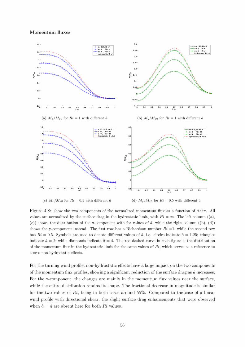
Momentum fluxes
0 0.1 0.2 0.3 0.4 0.5 0.6 0.7 0.8 0.9 1−0.2
0
0.2
0.4
0.6
0.8
1
1.2
1.4
` z//
Mx/M
x0
a = 1.25, Ri = 1a = 2, Ri = 1a = 4, Ri = 1hydrostatic, Ri = 1
(a) Mx/Mx0 for Ri = 1 with different a
0 0.1 0.2 0.3 0.4 0.5 0.6 0.7 0.8 0.9 1−0.1
−0.05
0
0.05
0.1
0.15
0.2
0.25
0.3
0.35
0.4
` z//
My/M
y0
a = 1.25, Ri = 1a = 2, Ri = 1a = 4, Ri = 1hydrostatic, Ri = 1
(b) My/Mx0 for Ri = 1 with different a
0 0.1 0.2 0.3 0.4 0.5 0.6 0.7 0.8 0.9 1−0.2
0
0.2
0.4
0.6
0.8
1
1.2
1.4
1.6
` z//
Mx/M
x0
a = 1.25, Ri = 0.5a = 2, Ri = 0.5a = 4, Ri = 0.5hydrostatic, Ri = 0.5
(c) Mx/Mx0 for Ri = 0.5 with different a
0 0.1 0.2 0.3 0.4 0.5 0.6 0.7 0.8 0.9 1−0.1
0
0.1
0.2
0.3
0.4
0.5
0.6
` z //
My/M
y0
a = 1.25, Ri = 0.5a = 2, Ri = 0.5a = 4, Ri = 0.5hydrostatic, Ri = 0.5
(d) My/Mx0 for Ri = 0.5 with different a
Figure 4.8: show the two components of the normalized momentum flux as a function of βz/π. All
values are normalized by the surface drag in the hydrostatic limit, with Ri =∞. The left column ((a),
(c)) shows the distribution of the x-component with for values of a, while the right column ((b), (d))
shows the y-component instead. The first row has a Richardson number Ri =1, while the second row
has Ri = 0.5. Symbols are used to denote different values of a, i.e. circles indicate a = 1.25; triangles
indicate a = 2; while diamonds indicate a = 4. The red dashed curve in each figure is the distribution
of the momentum flux in the hydrostatic limit for the same values of Ri, which serves as a reference to
assess non-hydrostatic effects.
For the turning wind profile, non-hydrostatic effects have a large impact on the two components
of the momentum flux profiles, showing a significant reduction of the surface drag as a increases.
For the x-component, the changes are mainly in the momentum flux values near the surface,
while the entire distribution retains its shape. The fractional decrease in magnitude is similar
for the two values of Ri, being in both cases around 55%. Compared to the case of a linear
wind profile with directional shear, the slight surface drag enhancements that were observed
when a = 4 are absent here for both Ri values.
56

However, for the y-component, besides the drop in the surface drag, non-hydrostatic effects
lead to a significant modification in the distribution of the momentum flux. When Ri = 1,
the y-component of the surface drag in the hydrostatic limit is about 0. So, the decrease
of the drag due to non-hydrostatic effects (when a becomes small, e.g 2 or 1.25) leads to a
negative y-component of the momentum flux near the surface. The y-momentum flux value
then increases with z and reaches a positive maximum at around the middle of the calculation
domain, as shown in figure (4.8(b)). However, when Ri = 0.5, since the y-component of the
surface drag increases to a larger positive value in the hydrostatic limit, then the decrease of
the drag value due to non-hydrostatic effects cannot bring its value down to below 0. So, the
overall y-component of the momentum flux remains positive throughout the atmosphere.
Moreover, compared to the corresponding result for the linear wind profile, the y-component
of the momentum flux does not show a significant drop by a factor of about 1/√
2. This is
because the turning wind profile turns by an angle of π within the first layer of the atmosphere,
so any wave number k has one critical level within the domain, which protects the upward-
propagating waves from the interference due to downward propagating waves. Hence, if a is
large, e.g. a ∼ 4, then the momentum flux profile tends to the hydrostatic limit, indicated by
the red dashed curves in figures (4.8(b)) and (4.8(d)). This also corroborates that the significant
reduction in the y-component of the momentum flux in the case of the linear wind profile is due
to the critical-level-free zone in the wave number plane, i.e. the orange region in figure (4.3),
in which all of the y-component momentum flux is reflected back to the surface by downward
propagating waves.
57
Chapter 5
Concluding remarks and future work
This dissertation explored the behaviors of two important quantities, namely the momentum
flux and surface drag associated with mountain waves generated by an isolated mountain, in
both the hydrostatic and non-hydrostatic regimes. In this chapter, the main findings will be
summarized in separate sections, and then followed by a description of possible future works.
5.1 Analysis of methods
Various approaches have been investigated and successfully applied. Assuming non-rotating,
linearized flow with the Boussinesq approximation, the exact solution to the mountain wave
problem for a linear wind profile with directional shear in the non-hydrostatic limit has been
successfully derived, which in theory is also valid in the hydrostatic regime by assuming that
the magnitude of the horizontal wave vector k12 is small. The exact solution is based on the
fundamental work by McFarlane (1987). The WKB approximation, which is only valid in hy-
drostatic limit, has been examined following the approach by Teixeira and Miranda (2004), and
similar results were successfully reproduced. The numerical method developed by Siversten
(1972) was also successfully manipulated and the results showed excellent agreement with the
WKB approximation in the case of a linear wind profile. With the aid of the exact solution for
the linear wind profile, the accuracy of the numerical method has been demonstrated, and hence
this method could be safely applied to the turning wind profile case. In the non-hydrostatic
limit, an alternative numerical method has been proposed and applied to calculate the wave
solutions for the turning wind profile. Both quantities of interest (the surface drag and the
wave momentum flux) have also been calculated using this alternative numerical approach.
58

5.2 Calculation results
5.2.1 Hydrostatic regime
In the hydrostatic limit, variations of the surface drag as a function of Ri−1 for the two wind
profiles exhibit different behaviors. For the linear wind profile, both components of the surface
drag keep decreasing throughout the range of Ri−1 from 0 to 4; while for the turning wind
profile the surface drag shows an increasing trend as Ri−1 increases. This difference is in fact
due to the absence of curvature in the linear wind profile. This conclusion can be reached by
analyzing the analytic drag formula obtained using the WKB approximation. However, the
WKB approximation fails to capture any variation of the y-component of the surface drag in
the turning wind profile. This is because the WKB approximation valid up to second order
can only provide a linear fit for the surface drag as a function of Ri−1 near Ri−1 = 0. But the
y-component of the drag near Ri−1 = 0 basically shows no variation, hence the WKB solution
predicts a constant value of 0 for this component.
Concerning the normalized momentum fluxes, for both wind profiles, a general decreasing trend
with height in the x-component can be observed, and the variations are similar, while the y-
components of the momentum flux for the two wind profiles take different values near the
surface and reach a maximum at different heights. Nevertheless, initial increasing trends can
be observed for the two wind profiles. For the linear wind case, the y-component of the momen-
tum flux takes a value close to 1 and a maximum occurs near the surface. But for the turning
wind profile, the y-component of the momentum flux takes small values near the surface, and
a maximum occurs in the middle of the calculation domain.
5.2.2 Non-hydrostatic regime
In the non-hydrostatic limit, the overall variation of the surface drag and momentum fluxes
becomes a-dependent, which means that the system becomes sensitive to the degree of non-
hydrostaticity. Moreover, due to the occurrence of wave reflection, both surface drag and
momentum fluxes show different behaviors. For the linear wind profile, the surface drag as a
function of Ri−1 shows a trend of non-linear increase when Ri is large, which corresponds in-
stead to a decrease in the hydrostatic limit. That non-linear behavior becomes more pronounced
when the system is more non-hydrostatic. Moreover, the surface drag values are significantly
reduced. That reduction is due to the effect of wave reflections occurring in the vicinity of
evanescent wave regions. This is more obvious in the y-component of the drag or momentum
flux, for which severe wave reflections occur for wave numbers which have their corresponding
critical levels below the surface. The substantial drop in surface drag is also associated with a
significant reduction in the momentum flux near the surface. But this effect does not modify
much the trend of variation of the momentum flux with height.
59

For the turning wind profile, a second layer of atmosphere is added on top of the original
calculation domain, which has constant static stability, density and basic wind. The basic wind
velocity in this additional layer takes the same value as at the top of the first layer so that con-
tinuity of the wind profile is guaranteed. Due to the periodicity of occurrence of critical levels
with height in the turning wind profile, the second layer avoids the complications arising from
the effects of multiple critical levels and wave reflections. In this atmospheric configuration, the
increasing trend of the surface drag as a function of Ri−1 which was observed in the hydrostatic
regime is suppressed when Ri−1 gets close to 4. This is caused by the stronger wave reflection
effect that occurs when Ri is small. This is also the reason why the variation of the surface
drag becomes more non-linear as the system becomes more non-hydrostatic. Concerning the
momentum fluxes, both components of this quantity show a large drop in magnitude near the
surface when the system becomes more non-hydrostatic. Besides this change, when Ri is large,
the y-component of the momentum flux near the surface takes negative values but changes its
sign to positive as z increases.
5.3 Overall effect of non-hydrostaticity
From the changes found in the investigation of the non-hydrostatic mountain wave system, the
general effect of non-hydrostaticity is that of causing a significant reduction to both the surface
drag and the momentum fluxes near the surface. Such a reduction is crucial, since current drag
parametrization schemes are mainly based on the hydrostatic assumption, which may thus over-
estimate the momentum and energy transport by terrain-generated gravity waves.
All the derivations and calculations carried out here assumed a non-rotating, inviscid, adiabatic,
linearized flow with the Boussinesq approximation. Diabatic and non-linear effects have all been
neglected for simplicity, since these effects may cause unnecessary complications in the adopted
conceptual model.
5.4 Future work
In the investigation carried out in this dissertation, there are three main lines of further work
that can be pursued. Firstly, the atmospheric setting for the linear wind profile in non-
hydrostatic conditions is in fact unrealistic due to the fact that in reality the basic wind mag-
nitude cannot keep increasing with z indefinitely. Typically, as the stratosphere is reached,
the atmosphere becomes much more stable and hence more favourable for wave propagation.
Hence, a two layer model for such a linear wind profile in non-hydrostatic conditions is worth
being considered to obtain a more realistic representation of the wave reflection effect due to
non-hydrostaticity. One significant modification relative to the present results should be that
the pronounced wave reflections for wave numbers with critical levels below the surface would
not occur anymore. Hence, the corresponding severe reduction of the surface drag and momen-
tum fluxes should also be suppressed.
60
Secondly, the maximum turning angle of the turning wind profile may also play an impor-
tant role in modifying the variation of the surface drag and momentum fluxes. When the basic
wind turns by an angle of π, all wave numbers have exactly one critical level within the domain.
However, this is clearly not always true for the real atmosphere. If the turning angle is less
than π, then some wave numbers will not have a critical level within the atmosphere, and hence
wave reflection may strongly affect those wave numbers. Therefore, the dependence of the drag
and momentum fluxes on the turning angle would be an interesting problem for investigation.
Thirdly, non-hydrostaticity can also be studied more thoroughly. Since a non-hydrostatic sys-
tem is a-dependent, quantities like the surface drag become dependent on both Ri and a. Hence,
accurate parametrization schemes for surface drag must capture that dependence as well, which
justifies investigating it in more detail.
61

Bibliography
Booker, J. R. and F. P. Bretherton, 1967: The critical layer for internal gravity waves in a shear
flow. Journal of Fluid Mechanics, 27 (3), 513–539.
Breeding, R. J., 1971: A non-linear investigation of critical levels for internal atmospheric
gravity waves. Journal of Fluid Mechanics, 50 (part 3), 545–563.
Bretherton, F. P., 1966: The propagation of groups of internal gravity waves in a shear flow.
Quarterly Journal of the Royal Meteorological Society, 92 (394), 466–480.
Broad, A. S., 1995: Linear theory of momentum fluxes in 3-d flows with turning of the mean
wind with height. Quarterly Journal of the Royal Meteorological Society, 121 (528), 1891–
1902.
Gil, A., J. Segura, and N. M. Temme, 2002: Evaluation of the modified bessel function of the
third kind of imaginary orders. Journal of Computational physics, 175 (2), 398–411.
Gil, A., J. Segura, and N. M. Temme, 2004: Computing solutions of the modified bessel differ-
ential equation for imaginary orders and positive arguments. ACM Transactions on Mathe-
matical Software (TOMS), 30 (2), 145–158.
Gregory, D., G. J. Shutts, and J. R. Mitchell, 1998: A new gravity-wave-drag scheme incorpo-
rating anisotropic orography and low-level wave breaking: Impact upon the climate of the
uk meteorological office unified model. Quarterly Journal of the Royal Meteorological Society,
124 (546), 463–493.
Grisogono, B., 1994: Dissipation of wave drag in the atmospheric boundary layer. Journal of
the atmospheric sciences, 51 (10).
Grubisic, V. and P. K. Smolarkiewicz, 1997: The effect of critical levels on 3d orographic flows:
Linear regime. Journal of the atmospheric sciences, 54 (15), 1943–1960.
Hines, C. O., 1988: A modeling of atmospheric gravity waves and wave drag generated by
isotropic and anisotropic terrain. Journal of Atmospheric Sciences, 45, 309–322.
Kim, Y. J. and A. Arakawa, 1995: Improvement of orographic gravity wave parameterization
using a mesoscale gravity wave model. Journal of the atmospheric sciences, 52 (11), 1875–
1902.
Lin, Y. L., 2007: Mesoscale dynamics. Cambridge University Press.
62
Lott, F. and M. J. Miller, 1997: A new subgrid-scale orographic drag parametrization: Its
formulation and testing. Quarterly Journal of the Royal Meteorological Society, 123 (537),
101–127.
McFarlane, N. A., 1987: The effect of orographically excited gravity wave drag on the general
circulation of the lower stratosphere and troposphere. Journal of the atmospheric sciences,
44 (14), 1775–1800.
Miranda, P. M. A. and I. N. James, 1992: Non-linear three-dimensional effects on gravity-
wave drag: Splitting flow and breaking waves. Quarterly Journal of the Royal Meteorological
Society, 118 (508), 1057–1081.
Nappo, C. J., 2012: An introduction to atmospheric gravity waves, Vol. 102. Access Online via
Elsevier.
Satyanaryanan, A. and P. L. Sachdev, 1980: Reflection of internal gravity waves in an atmo-
sphere with wind shear: Wkb approximation. Indian Journal of Pure and Applied Mathe-
matics, 11 (12), 1696–1703.
Shutts, G., 1995: Gravity-wave drag parametrization over complex terrain: The effect of critical-
level absorption in directional wind-shear. Quarterly Journal of the Royal Meteorological
Society, 121 (525), 1005–1021.
Shutts, G. J., 1998: Stationary gravity-wave structure in flows with directional wind shear.
Quarterly Journal of the Royal Meteorological Society, 124 (549), 1421–1442.
Shutts, G. J. and A. Gadian, 1999: Numerical simulations of orographic gravity waves in flows
which back with height. Quarterly Journal of the Royal Meteorological Society, 125 (559),
2743–2765.
Teixeira, M. A. C. and P. M. A. Miranda, 2004: The effect of wind shear and curvature on
the gravity wave drag produced by a ridge. Journal of the atmospheric sciences, 61 (21),
2638–2643.
Teixeira, M. A. C. and P. M. A. Miranda, 2006: A linear model of gravity wave drag for hydro-
static sheared flow over elliptical mountains. Quarterly Journal of the Royal Meteorological
Society, 132 (620), 2439–2458.
Teixeira, M. A. C. and P. M. A. Miranda, 2009: On the momentum fluxes associated with
mountain waves in directionally sheared flows. Journal of the Atmospheric Sciences, 66 (11),
3419–3433.
Teixeira, M. A. C., P. M. A. Miranda, and J. Argaın, 2008: Mountain waves in two-layer
sheared flows: Critical-level effects, wave reflection, and drag enhancement. Journal of the
Atmospheric Sciences, 65 (6), 1912–1926.
Teixeira, M. A. C., P. M. A. Miranda, J. L. Argain, and M. A. Valente, 2005: Resonant
gravity-wave drag enhancement in linear stratified flow over mountains. Quarterly Journal of
the Royal Meteorological Society, 131 (609), 1795–1814.
63

Teixeira, M. A. C., P. M. A. Miranda, and M. A. Valente, 2004: An analytical model of
mountain wave drag for wind profiles withshear and curvature. Journal of the atmospheric
sciences, 61 (9), 1040–1054.
Thompson, I. J. and A. R. Barnett, 1985: Coulcc: A continued-fraction algorithm for coulomb
functions of complex order with complex arguments. Computer physics communications,
36 (4), 363–372.
Whitten, R. C. and C. A. Riegel, 1973: Internal gravity waves in an atmosphere with wind
shear: Validity of the wkb approximation at critical layers in the presence of buoyancy forces.
Journal of Atmospheric Sciences, 30, 313–316.
Wurtele, M. G., R. D. Sharman, and T. L. Keller, 1987: Analysis and simulations of a
troposphere-stratosphere gravity wave model. part i. Journal of Atmospheric Sciences, 44,
3269–3281.
64

Appendix A
Behavior of gravity waves near a
critical level
In this section, we will examine the behavior of gravity waves near a critical level by using the
approach of Frobenius expansion. This analysis follows the treatment presented in the book by
Nappo (2012) and we extend the idea a bit further to the case of a three-dimensional isolated
mountain.
In the Taylor-Goldstein equation (A.1), the critical level is defined to be the height zc at which
the denominator, U · k = U(z)k1 + V (z)k2, is zero. This means that at the critical level,
the unperturbed wind U(z) is perpendicular to the horizontal wave vector k. This produces
a singularity (a second-order pole) in the Scorer parameter in equation (A.1), and hence the
first-order derivative of w(z) is not continuous at the height zc. Moreover, note that the square
of the Scorer parameter l2 is proportional to the square of the vertical wave number m of the
gravity waves. As z approaches zc, the Scorer parameter blows up to infinity. This implies that
the gravity waves becomes highly oscillatory, as will be shown in the following discussion.
d2w
dz2+(l(z)2 − k212
)w = 0 (A.1)
where l(z)2 is the square of the Scorer parameter, defined to be
l(z)2 =N2
(U · k)2+
U′′ · kU · k
(A.2)
Assume that we approach the critical level from above: then near the critical level, we write
z = zc + ξ, where ξ is assumed to be a small positive distance from the critical level zc. For
convenience, define G(z) := U(z) ·k. We expand the function G(z) near zc by Taylor expansion
G(zc + ξ) = 0 +G′(zc)ξ +1
2G′′(zc)ξ
2 +O(ξ3) (A.3)
65

Then, the square-root of the denominator in equation(A.2) can be approximated as
1
G(zc + ξ)≈ 1
G′(zc)ξ + 12G′′(zc)ξ2
=1
G′(zc)ξ(1 + G′′(zc)2G′(zc)
ξ)
≈1− G′′(zc)
2G′(zc)ξ
G′(zc)ξ(A.4)
Since we only consider simple linear and turning wind profiles, and the curvature term−G′′(z)/G(z)
is constant in both cases, we use β2 to denote this term. Thus, the square of the vertical
wavenumber (or l2 − k212) of the waves becomes
N2k212
(1− G′′(zc)
2G′(zc)ξ)2
ξ2(G′(zc))2+ β2 − k212
=N2k212
(G′(zc))2
(1
ξ2+
(G′′(zc)
2G′(zc)
)2
− G′′(zc)
G′(zc)
1
ξ
)+ β2 − k212
=Ri
ξ2− α
ξ+ γ (A.5)
where Ri =N2k212
(G′(zc))2actually has the same scale as the Richardson number Ri, α = Ri
(G′′(zc)G′(zc)
)and γ = Ri
(G′′(zc)2
4G′(zc)2
)+ β2 − k212.
Rewriting equation(A.1), we have
d2w
dz2+
[Ri
ξ2− α
ξ+ γ
]w = 0. (A.6)
The asymptotic behavior of w(z) near the critical level zc can be solved using a Frobenius
expansion, by assuming w(zc + ξ) can be written as
w(zc + ξ) =∞∑n=0
Cnξn+λ (A.7)
Substitute equation (A.7) into equation (A.6), expand and group the coefficients of powers of
ξ.
[λ(λ− 1) + Ri]C0ξλ−2+
[λ(λ+ 1) + Ri]C1 − αC0ξλ−1+
[(λ+ 1)(λ+ 2) + Ri]C2 − αC1 + γC0ξλ + ... = 0 (A.8)
66

Thus, we require all the coefficients to be zero, and this yields the following relations
C1 =
(α
λ(λ+ 1) + Ri
)C0, (A.9)
C2 =
(α2[λ(λ+ 1)]−1 − γ(λ+ 1)(λ+ 2) + Ri
)C0 (A.10)
and importantly
λ2 − λ+ Ri = 0 (A.11)
Actually, for both the two considered wind profiles, α is 0, since the linear wind profile has no
curvature, and the simple turning wind profile has w′′(zc) = −β2w(zc) = 0, so some further
simplifications can be achieved, but this will not be presented here.
Equation (A.11) gives,
λ± =1
2± iµ (A.12)
where µ =√Ri− 0.25. These two branches of λ correspond to the two members of the solution
basis, and the general solution near zc (up to second-order) can be written as
w(zc + ξ) = C+0 ξ
λ+A(ξ) + C−0 ξλ−A∗(ξ) (A.13)
where A(ξ) = 1 + C1C0ξ + C2
C0ξ2.
Thus, equation (A.13) gives the asymptotic behavior of w just above the critical level. The fac-
tor ξλ± can be written as√ξe±iπ ln ξ, which is highly oscillatory due to the fact that ln ξ → −∞
as ξ → 0. Figure(A.1) shows this behavior of w(z) near the critical level.
Real part of w(z)imaginary part of w(z)
Figure A.1: Behavior of the real and imaginary parts of w(z) on one side of the critical level, which is
indicated by the vertical red dotted line.
We are now at the right point to extend this solution, i.e. equation(A.13), to below the
critical level, but this is not as simple as it seems. For z just below zc, we may write z = zc− ξ,
67

and rewrite equation (A.13), just by replacing ξ with −ξ, that is
w(zc − ξ) = C+0 (−ξ)λ+A(−ξ) + C−0 (−ξ)λ−A∗(−ξ) (A.14)
However, a tricky point comes from the terms (−ξ)λ± . This is because Re(λ±) = 12 , but −ξ is
now negative. This will lead to two branches of possible solutions, due to the fact that (−1)1/2
can be either i or −i, and we have to decide which branch to choose. This ambiguity can be
solved by introducing an artificial damping term to the original Taylor-Goldstein equation, and
let the damping magnitude tend to zero, to see how the solution approaches this limit.
Now, we introduce a small imaginary phase speed ici, where ci is a small positive quantity.
Then zc is no longer a singularity, but this can be recovered by letting ci → 0. By doing this,
the Taylor-Goldstein equation becomes
d2w
dz2+
[N2
(ici −G(z))2+ β2 − k212
]w = 0 (A.15)
Assuming again that we approach the critical level from above, so that z = zc+ξ, the dominant
behavior of equation (A.15) is
d2w
dz2+
[Ri
(z − zc − ici/G′(zc))2
]w = 0 (A.16)
Then, by equation(A.13), the asymptotic behavior of w(z) (up to zeroth-order) is
w(ξ) = A(ξ − i ciG′(zc)
)1/2+iµ +B(ξ − i ciG′(zc)
)1/2−iµ (A.17)
Now, we go across the critical level to z < zc, and examine the behavior of (−ξ − i ciG′(zc)
)1/2±iµ
as ci → 0. We can see that, fixing −ξ, if G′(zc) > 0, then (−ξ− i ciG′(zc)
)→ e−iπ as ci → 0. This
is because in this case (−ξ − i ciG′(zc)
) would always stay in the third quadrant of the complex
plane and move towards the real axis as ci → 0, as shown in figure (A.2).
!𝑧! − 𝜉 ,−𝑐!
𝐺!(𝑧!)!
𝑧!
−𝑐!
𝐺!(𝑧!) −𝜉
𝜃 0
𝑅𝑒
𝐼𝑚
Figure A.2: Location of (−ξ− i ciG′(zc)
) in the complex plane (indicated by the blue dot) and the
critical level zc (indicated by the red dot on the real axis).
68

Thus, for G′(zc) > 0
(−ξ)λ± = e−iπλ±ξλ±
= e−iπ2 e±πµξλ±
= −ie±πµξλ± (A.18)
Similarly, for G′(zc) < 0, we have (−ξ − i ciG′(zc)
)→ eiπ as ci → 0
(−ξ)λ± = eiπλ±ξλ±
= eiπ2 e∓πµξλ±
= ie∓πµξλ± (A.19)
In general, by letting sgn = sign(G′(zc)), we can write (−ξ)λ± as
(−ξ)λ± = −i(sgn) e±(sgn)πµξλ± (A.20)
And therefore the overall solution w(z) for the entire positive z axis can be summarized as
follows
w(z) =√
(z − zc)(Aeiµ ln (z−zc) +Be−iµ ln (z−zc)
)for z > zc
(A.21)
w(z) = −i(sgn)√
(zc − z)(Ae(sgn)πµei ln (zc−z)µ +Be−(sgn)πµe−i ln (zc−z)µ
)for z < zc
(A.22)
Both parts of the solution are linear combinations of the two basis members (with coefficients
A and B multiplied). However, the behavior of the two basis members across the critical level
is different: one is amplified by a factor of eµπ, while the other is reduced by a factor of e−πµ,
depending on the value of sgn. It can be proved by determining the direction of the group
velocity that the branch with amplitude factor of eπµ multiplied for z < zc is always associated
with upward propagating energy, while the other branch is always associated with downward
energy propagation.
In chapter 1, we had shown that a gravity wave has upward propagating energy if and only if
the vertical wave number m has the same sign of Uk1 + V k2. For upward propagating energy,
consider now sgn > 0 and the term with coefficient A, near the critical level. The vertical wave
number m can be approximated as
m = −i w′
w∼ 1
z − zc
(µ− i
2
)for both z > zc and z < zc (A.23)
So it can be seen that Re(m) has the same sign as z− zc for the term with coefficient A. Now,
since sgn > 0, so Uk1 + V k2 > 0 above zc, and Uk1 + V k2 < 0 below zc, thus Uk1 + V k2 also
has same sign as z − zc. Therefore, Re(m) has the same sign as Uk1 + V k2 for the term with
69

coefficient A if sgn > 0, thus it is associated with upward propagating energy. Similarly, it can
be proved that if sgn < 0, the term with coefficient B is associated with upward propagating
energy. Therefore, we see that the terms with eπµ multiplied for z < zc always have upward
propagating energy. The proof follows the same reasoning for waves with downward propagat-
ing energy.
This is a significant result, since it means that the critical level always filters the wave by
multiplying it with a factor of e−πµ as it crosses the critical level in the direction of energy
propagation. In other words, it is possible to write the solution as a better combination of
the basis members such that sgn is not multiplied with eπµ, so that the direction of energy
propagation can be seen more clearly.
w+(z) =√
(z − zc)(C↑ei(sgn) ln (z−zc)µ + C↓e−i(sgn) ln (z−zc)µ
)for z > zc
(A.24a)
w−(z) = −i(sgn)√
(zc − z)(C↑eπµei(sgn) ln (zc−z)µ + C↓e−πµe−i(sgn) ln (zc−z)µ
)for z < zc
(A.24b)
In this way form, the term with coefficient C↑ in (A.24b) is always multiplied by the factor eπµ,
thus it is associated with upward propagating wave energy, while the term with coefficient C↓
is always multiplied by the factor e−πµ, which is associated with downward propagating wave
energy.
70

Appendix B
Definition of Fourier integrals and
the Parseval Theorem
The following definition of Fourier transform of an integrable function f(x) in (−∞,∞) is
adopted in the discussions of all the chapters,
f(k) =1
2π
∫ ∞−∞
f(x)e−ikxdx and (B.1a)
f(x) =
∫ ∞−∞
f(k)eikxdk, (B.1b)
where f(k) is the Fourier transform of f(x) and k is the wave number. With the above definition
of Fourier integrals, the Parseval theorem can be formulated as follows
1
2π
∫ ∞−∞
f(x)g∗(x)dx =
∫ ∞−∞
f(k)g∗(k)dk, (B.2)
where g(x) is also an integrable function in (−∞,∞), g(k) is the Fourier transform of g(x)
and the superscript ∗ denotes the complex conjugate. The proof of the theorem is sketched
as follows. By using equation (B.1b) for f and g, the left-hand side of equation (B.2) can be
written as
1
2π
∫ ∞−∞
f(x)g∗(x)dx =1
2π
∫ ∞−∞
(∫ ∞−∞
f(k1)eik1xdk1
)(∫ ∞−∞
g∗(k2)e−ik2xdk2
)dx (B.3)
Rearranging the integrals by moving the integral of x, we have
1
2π
∫ ∞−∞
f(x)g∗(x)dx =
∫ ∞−∞
∫ ∞−∞
f(k1)g∗(k2)
(1
2π
∫ ∞−∞
ei(k1−k2)xdx
)dk1dk2
=
∫ ∞−∞
∫ ∞−∞
f(k1)g∗(k2)δ(k1 − k2)dk1dk2, (B.4)
71

where the last equality uses the definition of the Dirac delta function. Then,
1
2π
∫ ∞−∞
f(x)g∗(x)dx =
∫ ∞−∞
f(k1)
(∫ ∞−∞
g∗(k2)δ(k1 − k2)dk2)dk1
=
∫ ∞−∞
f(k)g∗(k)dk, (B.5)
where the last equality uses the integration property of Dirac delta function. Hence, result
(B.2) follows.
72