draft - us environmental protection agency · draft appendix e existing data appendix f surface...
TRANSCRIPT

DRAFT
APPENDIX E
EXISTING DATA
APPENDIX F
SURFACE GEOPHYSICS
APPENDIX G
MONITORING WELL DATA
Afi3Q3f18

ill Appendix E
Existing Data
Lr:
flR303i 19
El
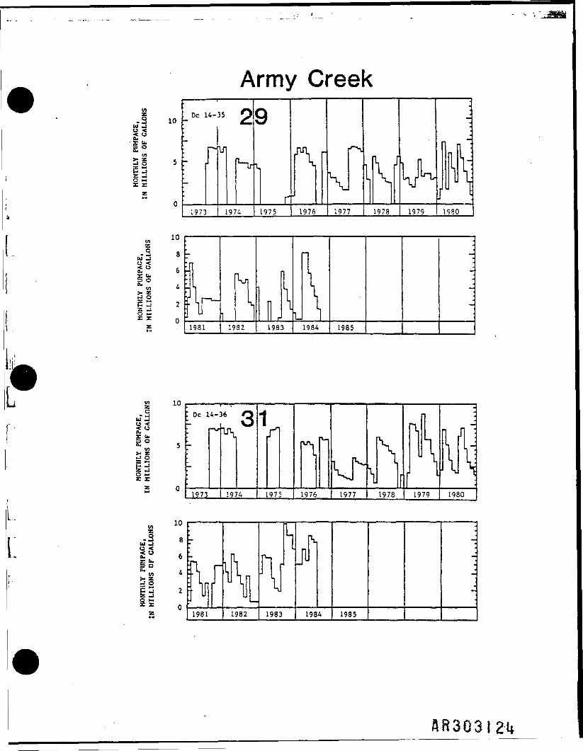
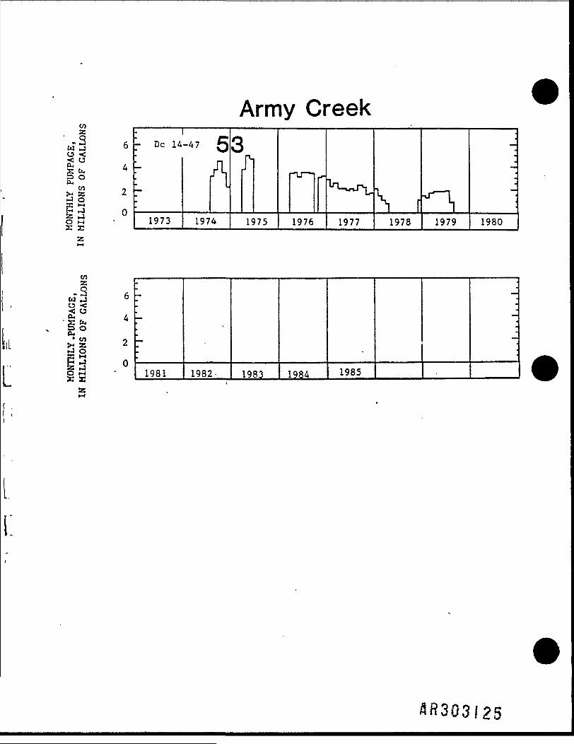
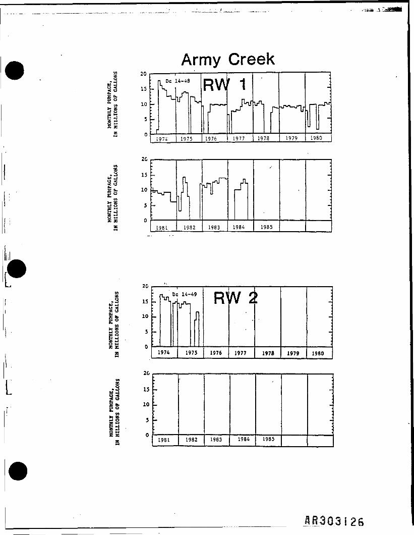
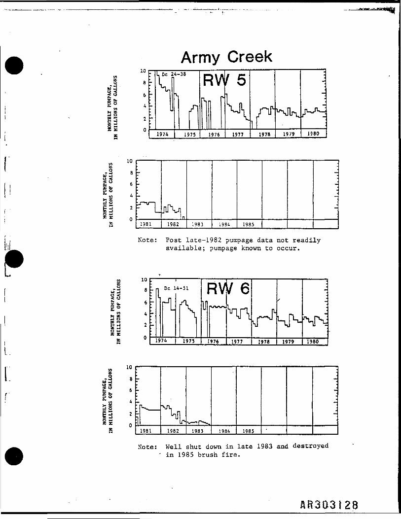
Groundwater Pumpage Histograms
L
RR3Q3120
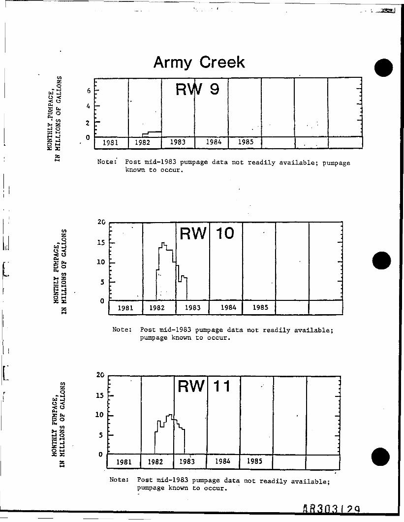
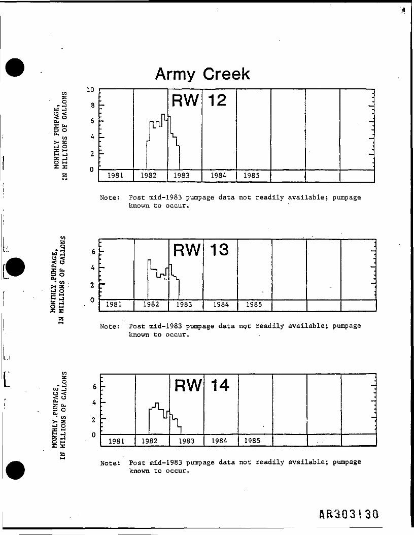
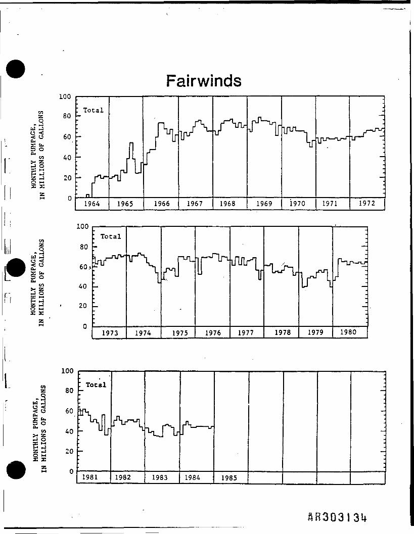
Note: Groundwater pumpage histograms provided hereare as complete as possible up to late 1984when the data was compiled. In some cases,more recent data was available and the histo-gram has been extended.
L
L
flR303!2l
v:zO- »Ju j
0 << uO,
to>• z-I Oa >-»H ^3O 1-1S S
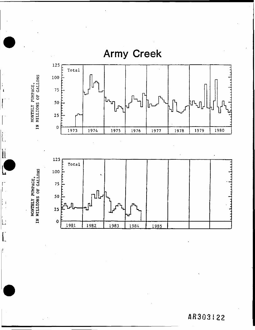
Army Creekl/D
100
75
50
25
0
; Total-
- r1973
Jhl_r
1974
Nv\1975
^T
1976
LA1977
JV1978
J -
1979
-
1
—
—w-
1980
125
AB303I22
£ b.S o
-i
Army CreekU _J<«
en>> z
-Jl"4
z
z- 10-3 8
U4 JO <£u 6x "•5 OE« 4> zJ O35 H* _p j 2
01981 1982 1983 1934 1985
1975 1976 1977 1978 1979 1980
1°si 8§ 6o
j oZ -1o *-*xx 0z 1981 1982 1983 1934 1985
^303123
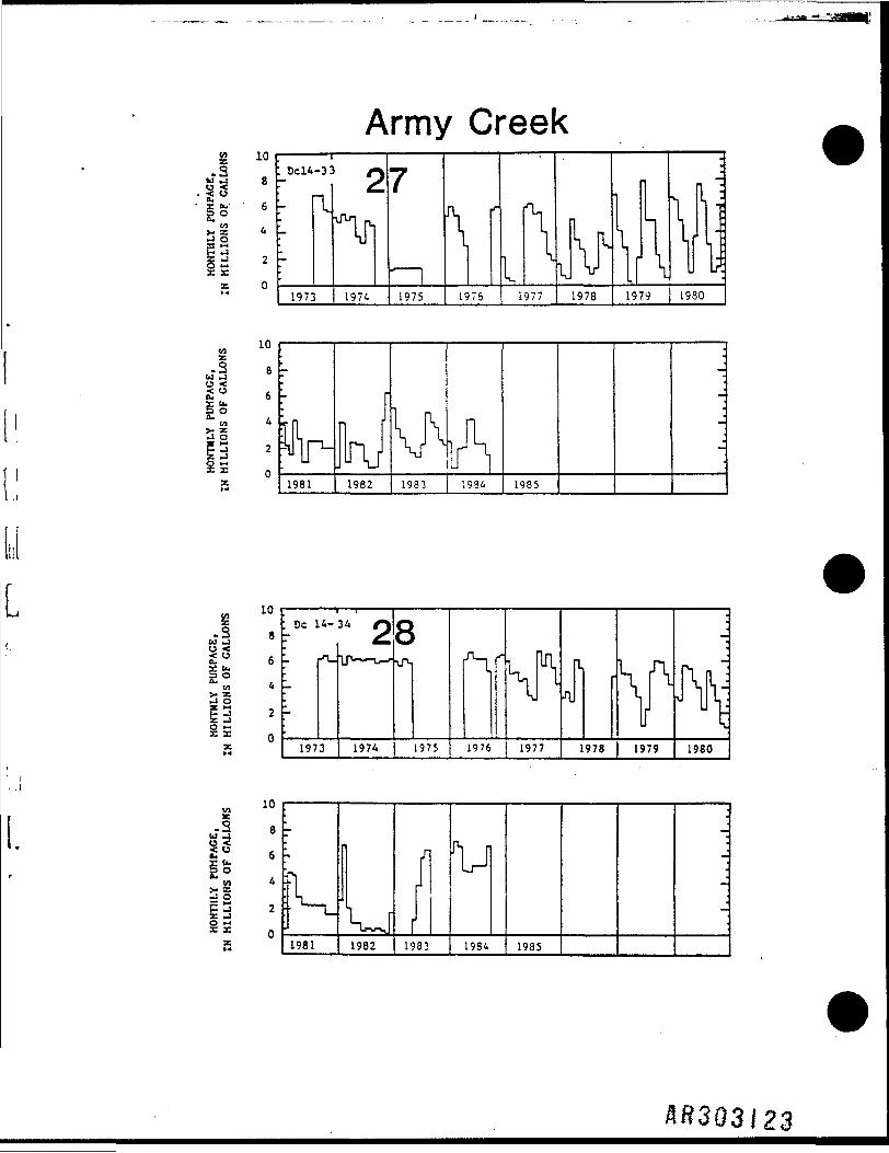
Army Creek.§ 10u u
• Z U.5 o
o •-•x x
DC 14-35 O
- r1973
IT
Sr
1974
9
V.
r1975
Pi1976
\.
• l
1977
,J
VJ
1978
gu1979
-j
^r i1980
1981 1982 1983 1984 1985
10-3u _io <
>* z-1 O
Z -JO —X Xz o« w
en 10
„-! 8
DC 14-36
1973 1974
1n
J975_ 1976 1977 1978 1979 1980
o *•xx1981 1982
jfl1983 1984 1985
COzU _)o •<2°• CO
>* Z•J OEC M
O MS X
Army CreekCO
6
g*. *5 oco o>- SB 2,4 o
13 0o M
1- DC 14-47 §
-
1973
A1974
3f
1975
nff
1976
In-• x1977
\ I1978
-J" —— 1
1979
—
-
1980
2
0
.
1981 1982- 1983 1984 1985
-
SR303I25
20„ a - De 14-4825 is
w 10s§13 5£x5 o
Army Creek/w n_1974 19751976 19771978 1979 1980
20u>
Ais 10|2 5XX 0
1981
Y"1982 1983 1984 1985
20in
| 15
8 10
1 5.jx 0
-
VLDC_r
1974
14-49
J
1975
R^
1976
N'.
1977
;
1978 1979
-
1980
20«n
jl 15
Is 10P O<n
k* K13. 'Z .4Ix 0z»4
1
-
'
—
1981 1982 1983 1984 1985
-
-
5130.3126

Army Creek
MONTHLY PUMPACE,
MOMTM.Y PItHPACE,
.„ mLLIONs' OP"ALLONS
IH MILLIONS OF GALLONS
IN HILLIONS
OF GALLONS
IH MILUONS OF
GALLONS
IH HILLIONS
Of CALLOHS
0 ~
- «" »
S ..
M ~ ~
..
e K '
s -tt
)
)
)
5
0
5
0
5
0
LO
8
6
4
2
0
2<
|f
1974
.-3
U
6
X
1975
R\
1976
V £
in/l/
1977
v^Ji1978
•tf[rs -
1979
-ifV -,
1980
;-
r1981
Note:
V,
[l
L"V1982
,
1983 1984 1985
-
Post late-1983 pumpage data not readilyavailable; pumpage known to occur.
DC
1
1974
U1981
14-
J
51
V1975
1URVwxrvr\
1976
^•
1982J——«J
1983
14Hr\1977
— -l -1984
^1978
1985
4J1-1979 1980
-
AR3Q3I27
en
.1
enSiSMX
.3U _!
-3
Army Creek
enz-3 aU -1o <£» 6X <"•? °cu /en 4>- zJ 0P3 2Z -Jo —rz 0Z»4
—
^
iv
1
1981
JiTVi! n
1982 1983 1984 1985
_
_J
-
•_
-
Note: Post late-1982 pumpage data not readilyavailable; pumpage known to occur.
10
8
6
4
2
0
-
-
—
IDC 1
pjj
1974
4-51
f\
1975
RV)/ 6u uuw%,
1976
VTA1977
r-J1si1978
UN1979
-j
n, r ~:
1980
s 10
!B1931 1982 1983 1984 1985
Note: Well shut down in late 1983 and destroyed' in 1985 brush fire.
•..
S5-3U _}
•3 Den
IIPg fj|
§ Xas
.3U J
§3On
CO
il
Army CreekUJZ
w§ 6o << oso, 45 o• 01 ,:« as *K 0
Id °£5 M '£ £
^
1981
-
1982
RV
1983
7 Q
1984 1985
-
asM Note: Post mid-1983 pumpage data not readily available; pumpage
known to occur.
.u
15
10
5
0
•
-
1981 19
pi..
82
F
IT,
1
?w
L983
10
1984 1985
-
Note: Post mid-1983 pumpage data not readily available;pumpage known to occur.
iV/
15
10
5
0
.~*
—
^
•
1981r
1982
RW
V
1983
11
1984
'•
1985
•
—
-
-•
Note: Post mid-1983 pumpage data not readily available;pumpage known to occur.
Army Creekw
.1 8U Jo << 0 ,eu 6
-w 4>« zJ O£ 3 2z uO »-4
0z
™*
_
—
1981 1«
__il_njuJ
)82
F^
(1*•
H
1W
)83
12
1984 1985
-
"•
_
.
Note: Post mid-1983 pumpage data not readily available; pumpageknown to occur.
zw § 6o <g 0
• tn oS Zg!j 0«jO MX X
_
-
—
1981 1
V382
RW;111983
13
1984 1985
_
-
•"
Note: Post mid-1983 pumpage data npt readily available; pumpageknown to occur.
z
o <2" A
•J o1= 5 °O 1-1X X
_
••
1981 1982.
RW
^1983
14
1984 1985
—
~
Note: Post mid-1983 pumpage data not readily available; pumpageknown to occur.
RR3Q3I
.3Ul _3O <•< O0-,
5 oto5>- Z
J O
Xs:
Airport Industrial Park
II
tu
15
10
50
40
3C
10
0
5
D
—
—
: T
r.1984 1985
-
-
-
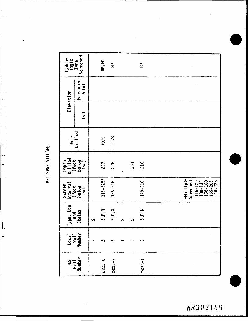
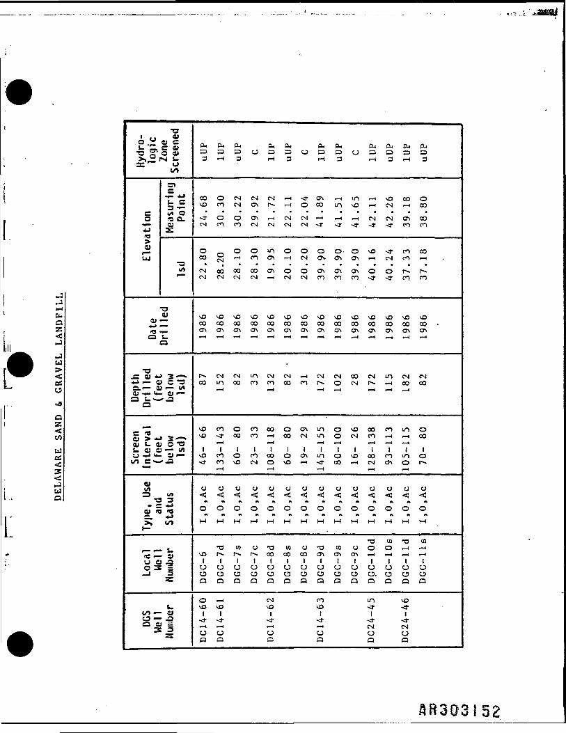
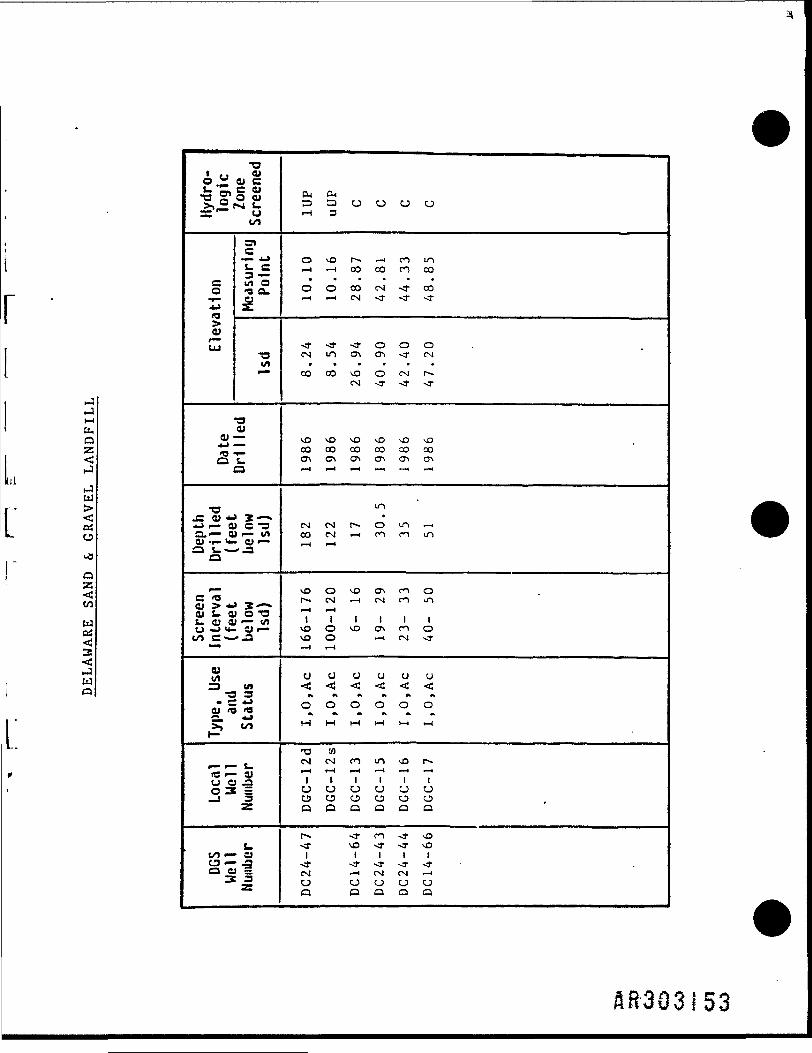
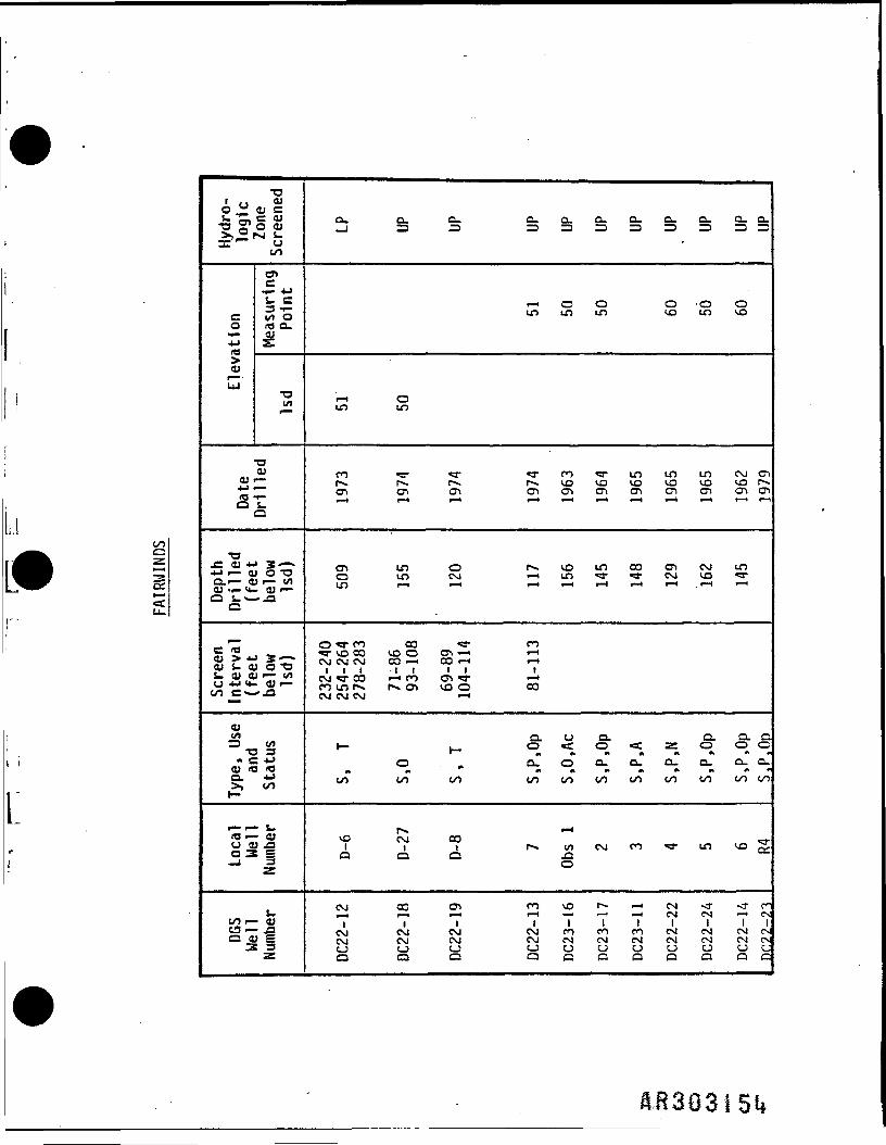
Artisans Village
r j
1980
r1981
A•
1982
«V
1983
innLr
1984 1985
-
-•
f
8R303I3I

Amoco60
50enZ
w| 40
|° 3°tn
>• Z- 2 20z _i
zM
60
50enzj| 40
is 30en
il 20O i->X!c 10z»««
0
60
50en
.3 40P
if "xx 10
0
60
50to
si 40|S 30W
5J 2 20
O M" 10
1-1
0
10
0
Total*™
"
1964 1965 1966
——
•
1967
Total
_
-
-
1969 1970
• •__«•••__ •
1971
. ——
1972
;
—— ——
—
-.~
1968
1973
.
-
-
-
1974
.-.
Total
]rv^
J\
"\
Upp
1975
AITS\er Poti
1976
\Ti-\
>mac1977
^
^
\IN
1978
UuTX-
1979
_
j
"J~uw ;
1980
: Total
—
_
-
n._A1981 1982 1983 1984 1985
•
^
J
-
-
18303132

Crown Zellerbach3U
• t/l
SS£±4055>-o 30
1§ 20£ -J-J
5Z icc a
""
5:-V"
5iIsZo 3C
-J
S5 ico z
0
>
-
1950
™~
>
1960
-
1951
1961
t
!i
1952
1962
r ~ -i1953
1963
1954
1964
1955
1965
1956
1966
1957
1967
1958
1968
-_
}
-;
1959
*"
~
1969
TOTAI. K
KIIMLt
rilllPACi:.
IK H
ILLIOHS
Of O
AlinwS
«-•
IV*
\ft
l»
Uo
o
o
o
o c
f-
1970 1971 1972 1973 1974 1975 1976 1977
L
1978
—41979
HCWIIU PWVACt.
LL10
MS O
f GALimS
^^J uj
A
uo o o c
2s 10a E
0
w>1980
•
Lr>— T"
1981 1982v-1983
-- --
1984——— |1985
-
-•
i
fl-8383133
Cu§a,
Fairwinds100
Totalz 80 '.3« j< u 60X t"S o&- ..2 40
20
01964 1965 19661967 1968 1969 1970 1971 1972
100
2 80o
2 ° 60.«X tu5 oo-
J oX t-tgd . 20x xz
0
I
1973 1974 19751976 1977 1978 1979 1980
100
z 80
o 60
en 40
: Total
S M 20X Xz
1981 1982 1983 1984 1985
AB303I3I*
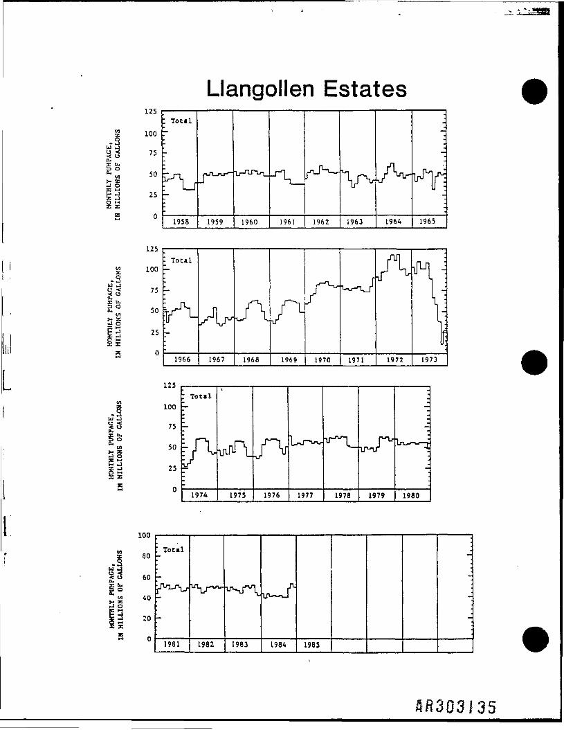
Llangollen Estates125
I Total100 r
UJ .JO < T,•< U 'J6.§0,O
50>• z-J O
1958 1959 1960 1961 1962 1963 1964 1965
U _!U •<•< O0,
sen
xz
125Total
100
75
50
25
01974 1975 1976 1977 1978 1979 1980
1UU
z 803S 60o
1j :oXaei- o
I Total
•-
-
1981
ut^ ——
1982
-if T\
1983 1984 1985
•
•-
•
•-
!

>. zs!2
en
.1u Ju 3
2§3Is
en
.3
ot/i
Midvale25
Total
20
15
1958 1959 1960 1961 1962 1963 1964 1965
20v>
AS"is 10
1981 1982 1983 1984 1985
JIB303I36
zu§o <
Zo
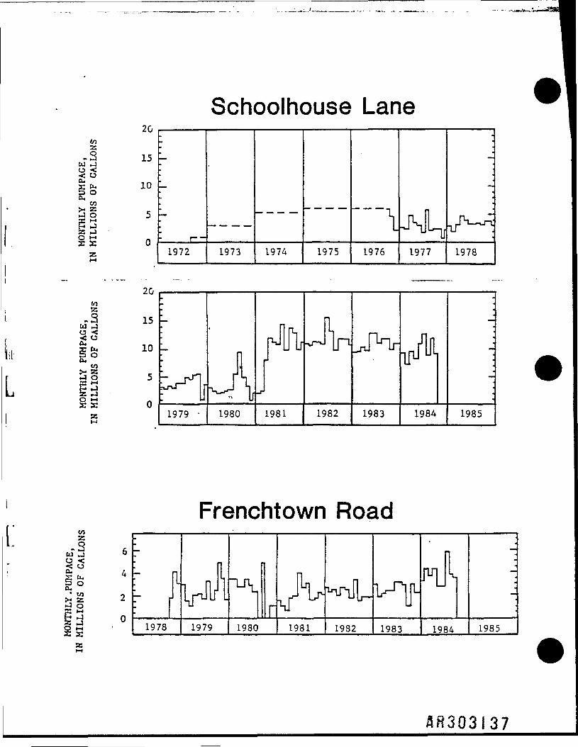
Schoolhouse Lane20
-3 15tu »jo << ox fa 10p o
O MXX
2060
M 1 15
x fa 105 Oto
So 5
O >H .xx 0
1972 1973 1974 1975 1976 1977 1978
1979 1980 1981 1982 1983 1984 1985
Frenchtown Road
w • 1978 1979 1980Xz
1981 1982 1983
I1984 1985
«8303I37

'E2
WELL CONSTRUCTION DATA
L;
L
ftR303!38
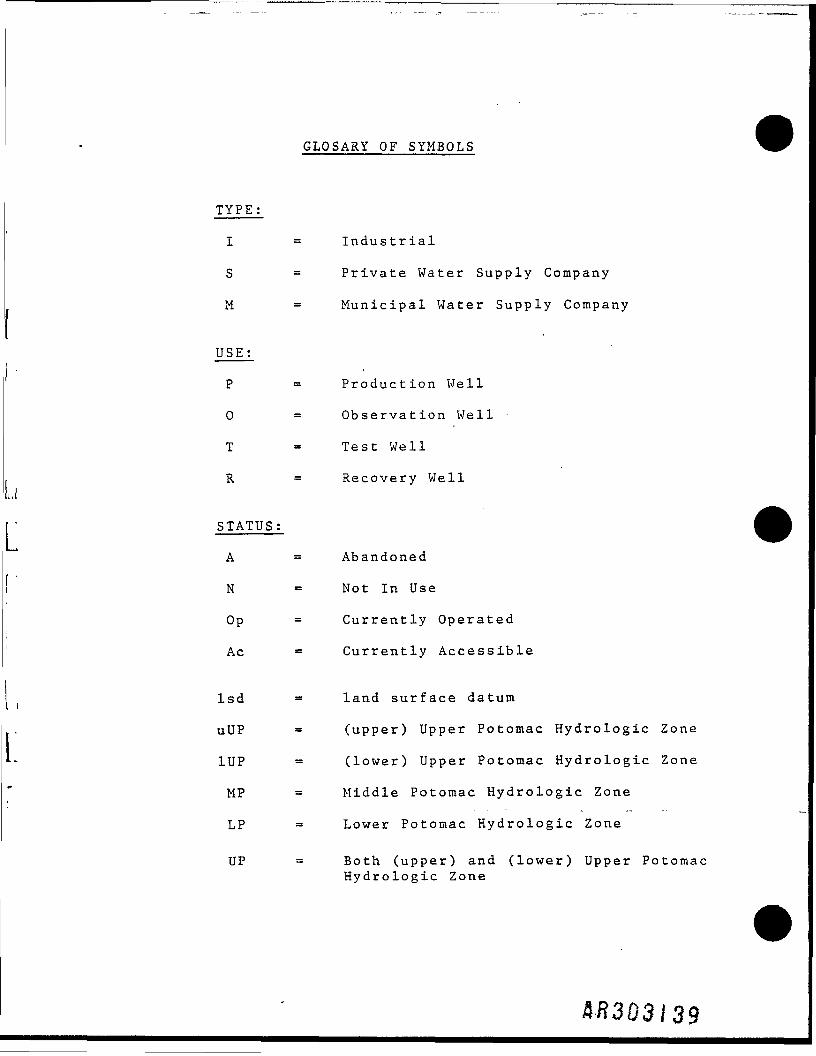
GLOSARY OF SYMBOLS
TYPE:
I - Industrial
S - Private Water Supply Company
M - Municipal Water Supply Company
USE:
P = Production Well
0 = Observation Well
T - Test Well
R - Recovery Well
STATUS:
A s Abandoned
N = Not In Use
Op - Currently Operated
Ac = Currently Accessible
Isd 3 land surface datum
uUP - (upper) Upper Potomac Hydrologic Zone
1UP - (lower) Upper Potomac Hydrologic Zone
MP - Middle Potomac Hydrologic Zone
LP = Lower Potomac Hydrologic Zone
UP - Both (upper) and (lower) Upper PotomacHydrologic Zone
4.8303139
Lf !
ooo
It'
c0•r--t->
(U
OIfOo
•o4T O) **j i— aCLr— fl
o
S > *<u s. as- 01 cC/> C«-
inT
* Cai tCL>i
,_ u a0 3_i
1/1 <-ts i-C £
5 a;vj i_
oo
cncS_ Cin O<TJ a.s-a
•aCJ
.ua
J C * fcj o -a. OJ i—
j 3.-.J O T3J *•"• e/>
'
in3 33 K3•MCO
• OJJ -Q
^
• Sj c=E 3Z
a. a.— i 3
o
CMCM
O CMCM CM
O —110 <ncn cnf— * f— 4
CO COo inIO i— i
co co cnm in •— ii i ico co eo«— l «3- CMin in «— i
Q.Z O*— a.*«4 »""H
n ro3 3O 0-
1 1in in0 00 0
a.
LOoCOCM
cCM
Oent— 4
Oo<n
CD CT* enCM in tnin in unt t io o <no co inin in in
CL00.*-*
T™ *
3a.
oI — 41inGo
ex
CM00
0•
CN°ir-
ovncnt—
PCO«-*
in1CNi— i
u<:0*
3O
t
Q
a.=2
o•
U|
O.
roi — i
incnr— *
in»i-H
LO
CM
r— 1
CMCO
O
0**
*—«
in0
COi— ii
r-4f 1
CL_ l
OCO
Oen1™
^vnin
0 (co inin int iin CMcsj inun in
zH-*
^
CM
C
<niin
CM0o
Q.
in
inCM
inCM
rtcnf-H
f^*— '
cnmi— iicnCMi— (
a.0ex.™*
CM
O.
tinCM0Q
a.
CMCO
0CM
OCM
Ocnt— *
inCM•"-•
COr— t<— 11
CO<— 11— 1
o<:o•*
t — i31—
f— 41inuC3
CL,
minr--.1—4
in
ocni— t
cnCO•— '
inCO
iCO1— 1
u
o*—
CO31—
COF~4
1mi — toQ
Q_ID
in
COi— i
o
ocnt—
cnCO1-4
oCOf-H
1inCMt— i
«=co^
3h-
cn1inuc
Q.
^
in?— t
in
o
oNin
O)cIB
oCN1m
a
QZeC
LUUJ
CJ
>-
-oo.r- o> 1" o *~i i~=^ £
CD~* TiJ
S. E
C lrt OO Tj Cu
ir: ———————
CU
•oin
•o<Uo; •—
It3 f-O S-Q
•aJC CJ 4J 2*-~4-2 r— • CD O "OC.r— QJ i— i/)O S-—— ^2O
C <QC > 4-> Z-— »CU L* O O ~Os. a; cu i— in
~
OJtrt13 in
Q. •»->>> "
J5fz
S-to *•• cuO W Ez
n_ o_ n_Z3 -3 3rH rH 3
«sr o CMm i— i incn co m
CO
CO CO CO
cn cn cn
o r»» CM
O in co
i i if L[ OO
CO O Of— 1 1— 1
o" z CD"cc o: as« « • « « *
Cu=>rH
COCO
CM1 — 1
CO
cn
oCM
O1—4
inCO
QLOC£
Q.13r-l
CM
COCO
CO
cn
CM
cnCM
iCOoi—H
a.o«
Cu=53
CO«T
in
cnr-.cn
en
cnincnun
c.occ
Cu-3
3
^r*.m
roen>
r-l
m1
zo:
a.=3
r-l
*3"mCOCO
incn
in
in
0CM~*
-,,
<*•
Cu-3rH
0cnCTi
CO
cn
inin
CO
cn0*-H
z
°z
Cu-J
O1— 'CMr— 4
cnCM
c»-*
CO
en
oCM
o1—4
1O
Q.O
<*
Cu_3 '
cnCO
CM
enCO
COpv.en
o
0CM
O
C.o02
Cu_3
r- cnf — 4
OCMin1—4
CO
cn
oCO
COI-H
CO
a.o<*
Cu Cu— i -33
cnCO
rH CM
O
. °rH <3-rH CM
CO CO
en cn
m inr-i cn
CMm. cnO 1
l r-a\m
a. c.o c°i °;
r-l CM CO3 3 3ce cc a.
~zf *& COl l lr-H — 4 CNCJ CJ OO Q Q
Qi
Oml
0Q
in
oorolCNOo
inO£
F— 4
inI
< — i
°
r-.C£
CNml•j-CJQ
1
inlmCJa
cn
CO1COCM
Q
PV.CM
COCO
"*•f- *CJo
COCM
CO
1—4
0
enCM
inCO
a
•—4 mcn in
m •"*co -fi i
r, sa Q
flR303U|

rJM&H
QS<rJ
"O1 , , Olo " ca cS. JL C CJ•c x o <u>>,__IVl S-31 U
(O
cn..-" 4-1j_ ZZ3 -r-
S </> Oc -so-"Z £TJ ————————
CU
LU•3Ul
O)-U —
-O T-
c.
JZ CU 4J 2 -— »•J •— a c -3yj1^ u_ 'o •—£• — *•— •» 3a
£- rocu > 4J 3'->cu &_ ai o "Ss- cj sj •-" mU ——! 11- CJ r——CO C^-^
uin35 in
•S 3• Z 4J
|"5
ic •— aU il -S03 =_! 3
S_CO •— CJ
O i) "=3 3Z
P-i3rH
-KrHrH.
vO
Ooocni-H
in*
CM0rH
CNOi—41
CL0*oM
o1 — is"
CW
3
•Ko-co.in
OoocnrH
CMCN~ '
vOco
linvO
aO*oM
i — l
OS
Cu
3
•K<j-O
inrH
OoocnrH
OCOi—4
m oor cn1 lm r-«m oo
a0
**ortM
CNF— 4
OS
Cu
3
•KvOcn.VO
Om•in
o00enrH
mCMF—— 4
m CM<r i--I lm -a-co in
CLO*
O
M
CO
3«
CU
3
Ooocni— i
p .F— 4
r
VOoo1m
CL0*o
rH
F— 4
3OA
oS-iunou
exoH*

LL
az<i*iLULUCtfCJ
T31 ,, CUo !£ cu s±V, J— . SI 1>-o x1 o eu>,.__; P I s_
CO
cnc••— 4-1S- C
C in *0O ra Cu5 £<uLU •oin
i—
•aOJ
OJ i—fO •f""O s-o
•oJ= cu *J 2— -— i •— cu o "o0.1— tu •— m<1) i- H- O> i—a s-- — JDo
c to(U > 4J 2- — •cu i- cu o "ai- cu cu <• — inCJ 4J <*— QJ f—to c-— *.c
t—CUen33 tn•C 3• C 4-»
CU 10 190. 4J>» to
r— i— J_<C r— CUO CU «£3
Z
to •— <uC2 f— jQQ OJ g
^
Cu33rH
r— 4CM
CO
Op
CM
cn
mm
in<niinun
ut*
O
031—4
m1—4
f— 4
S
CL Cu Cu33 35 33rH rH 3
«3- co encn in r-4p* p1 r »
1—4 r— 4
o cn cop~ p~. p~«
l-H r— 4
CM CM CMp*x p r"»»en cn en
cvi cn inr— i cn inr— 1
in
r$ C3 S ^ .1 O m10 co «a-Ml
en
CJ CJ
O 0F> "
<c. «=: car-4 CM CM
P*. CO1 1
1——4 F— 4CJ CJa a
a. Cu a.33 33 33rH 33
in in cor-4 cn inCO CM CMr- 1 in in
o o ocn r-i F-•—i in in
CM CM CMP p . r*cn cn en
in vO cnco cn co
* '
in o«T CO CMCO r- CO
1 1 1in o CMCM P-»
*J* F— 4
^U CJ< «a:0 0
•t M
«C < caoo y r
cn or-l CM
1 1
CJ CJ
Cu33r-t
<n_,1 — 4
int— 4r— 4 '
CMP-.en
CM
O1o
PV.
u
o
in
eniCOr— 4CJo
Cu333
COp*.P<r
«3"in
COP*Xen
r
or— 4
OCO
<c0
F—— 1
CM
<J3CM
1CMOa
Cu 0433 D
CO vOoo cn•3- CSin -a-
CS*J" •— 1CM rHin <r
co <np-» r--en en
cn •->in oor-4 rH
«3- m mun o 10
4 ^cor-. CO 1—4
OU f£<z *o 0
CM COCM CN
r-x coCM CsJ1 1
CM CMCJ tja Q
Cu.33
cncnOin
CO1—4
cn
COr-.cn
in
COm
COCO
u
o
CM
cnCMiCMCJa
Cu
rH
r» 4
COr
COoin
COP*cn
f— 4
minCOo
o
o
mCM
oCO
tCM
8
Cu33r-l
inenCM«3-
cnCOenCO
COp**»en
in
m<n
oo
u
0
<nCM
r— iCO
1
CMCJC.
flR3Q3U3
LUUJ
CJ
•o1 . , OJo ,~ cu cW ^^ C QJ•§,0,52:-n uto
cn•f- 4->i- c3 f-
C i/l OO fO Cu£ £CJLU •oin
•o0)
CU ——4-> r—rr; i-O S.O
•o—— |JJl JUj , B
•«-> i— OJ O "OC.I— OJ r— in0 S-s-. -JOO
C idCJ > *J 2 *OJ S. CJ O TJi- O) cu f— inCJ 4-> U- OJ 1 ——to c — ».a
OJ33 CO•a 3• C •»->a. -M>, CO
<C r—— CU(J O) JS
i-t- r— J3o cu E3 3
a.33
cni — iCO*in
cn•<nun
cnPS.cn
OP--.
COiniin
CO
CJ
0
oCO
CMco1CMCJ0
Cu
3
enoin
10•1 — 4
COpN»
en
Of
oiniinCO
u
o
COCO
COco1CM
°
CJ
COCO
CO
m•o
COps*cn
CMCO
1— 1CM1O
u
o
P-.CO
CO1CMCJ
Cu33rH
COl — 4
Cj-CO
P-.•
cnco
cnp-%.en
Om
r— iin1—4
l— 1CO
u
o
COCO
cnlCMOQ
Cu333
COcccncn
pNfc
cn
O<n
oor— iiocn
CJ
o
c
COCM
1inCMCJ
Cu Cu33 33rH
rH inCO O
m <rCO •— i
vn r-»• •cn cocn •—!
«3- CMP*. Pv.cn en
0 «3-CO CM
in orH vo cnF-4 F-l P>-
m o ocn m P"»
r— 1
0 0
o o
CM m10
«• CMCM CM1 1m «3-CJ CJa o
Cu33r-H
1—4l — 4
10r— 1
O•
10
CMps*en
^CM
O1— 11—4
inof— 4
CJ
0
COCNJ1T
CJQ
Cu3D
q.CM
CMr— 1
O•
CM1—4
CMP-s
en
^CM
CcnoCO
u
o
CO
CM1"CJo
ftPr-l
COinun
cn•un
CM
cn
«rj>CM
Oi— 1r-H
0C31—4
CJ
O
cn
inCM1^£_JQ
Cu33
r-HCM
cn
cn•CO
CM
en
^CM
|"CO1
CJ
o
of— 4
IOCM1
•sT(j
°
Cu CL33 3D3 3
cn uncn r-icn PS*
o ocn P*S
CM CM
en cn
^ 3"CM CM
O 00PS. ini iO 010 in
CJ CJ< f.0 O
r-l CM1— 1 I—— 4
PS. COCM CM
1 1^ «sT
O CJa Q
W303UU
r
i:
•oi .. cuo .- cu cs- ri c cu13 S1 O CU Cu>i a psj S. 33
CO r-1
cnci- C O
a in o inO it) Cur £CULU O
in in
•ocu0) •— CM•Mr— ps.re -1— en
TJJ= cu •<-> 2 --4-> i — OJ O T3 '«•C.'— cu •— in CMO !-• — --Q
^c <o oQJ S- CD O "O 1t- cu O) "— in O<j 4.) u_ cu i— incn Cs_».c
CJin cj33 in «-r
T33 «- C -M O
r—
r— r— I./O •— OJU CU Jd COO 3 E «-•-J 3
s- cn(O r— OJ CMC2 r- .Q 1Q-i i 2
^ CJ
Cu333
CMr—4
CMCM
1—4
CMCM
CMps.en
in*«f
inPSkiinin
CJ
o
in1—4
OCOt^0o
Cu333
enCO
1—4CM
CO
r-HCM
CMps.cn
in«3-
or-H
1Oor-4
CJ•s:o
PS.1—4
CO1
*3-CJo
Cu3D3
COCOCOCM
PS.
cnCM
CMPS.en
un«*r
incni0cn
CJ
O
CTir—4
CMCO1^
CJo
Cu3D
CO•vT
CMr—4
*ror-H
cnPS.en
oCM
COr—4
1COPS*
CJeCO
r-4
PS.CO1«sf
CJa
Cu3Di — i
r-
r-
CO
m
coPS»en
CMCO
CO1—4
1COPS.
oeCO
CO
COCO
1•sT
CJa
Cu3DrH
r— 1cnenl — 4
0inr-H
coPS.cn
oin
inin
OCM
• r-H
O*£.O
CMCO
cnCOi«sT
CJC
a.3DrH
OPS.
PS,
<nin
COPS*cn
o
<ncnioin
CJ<o
CO
o1
«sT
a
Cu33
inr—4
O
•sTf*
COPS.cn
r— iT
oCO
1CMin
u<O
inCO
r-H•sT
1T
^
Cu3DrH
COCOCO
rr1—4
COPS*cn
10CO
or— 1
1OPS.
O<c
CO
Cu33rH
Of — 1,3.CO
1—4
COcn
COPS.cn
CMin
o
i0r—41—1
CJ<
O
o«sT
cnen1
CJQ
Cu Cu3D 33
r-l
in coCO PS.in coCO CM
«=r «*rPS. PS.
en cn
<n ops* CO
in oin ini io unCM cn
rH r—4
CJ 0< <O O
I-H COin in
CM «3-r— 1 I—I
1 1in coI-H CMCJ CJ0 0

LULU
CJ
I .1
•oi o tui- "£, C CJ>» o p5 2.in *~ tjto
cnt- 4->S- C3 i-c in O
O rs Cu£ £fO
aLU •oin
tuo •—o TO
•o-C QJ *•> 2-—«4-! I— OJ O T3CLI— cu r— mCU i- <*- OJ •—O i-s-*-Q0
C «3CJ i- CU O TJJ— CJ cu r— enCJ 4U» l|_ CU I—10 C»— -JS
t-M
cuin33 in
•O 3« C 4J
Q."* 2^ «*75 r QJ(J O) J30 3 E
tO r— OJ15 •— XIO OJ E3 3Z
Cu Cu33 3D
3
in enPS. ID, ,
r-l PS.in ^
m•in
«3- COPS. ps.cn en
p«. P-S.4—1 «*T
s %1-H 1— 11 1O IO1-H O
CJ CJ<c <:C2 3
«3" CM
in cnr-H rH1 1CO COCM CMCJ Oo a
Cu3D
i-HcnCO~
un•COIT
CMPS,cn
in«*T
OCO1—41OCM
CJ
O
1—4
C u C u C u C u C u C u C u C u C u C u3 D 3 D 3 D 3 D 3 D 3 3 3 - 3 3 3 3 - 3rH rH rH i-l , rH r-l
i n i - H c n i n i n i n cn «—i «r rfO <n co en CM •— i c-J CM •— i cn• • • • • • * • • •r H i n i o c M ' s f ' s r « r i n c o i n
«sT •— 4 l— 4 I— 4 rJ CM «sT
P S . I — I C n O C M r — 4 F — 1 O r H I O• • • • • • • • • •O u n i n « — i c M C M < r c o u n t s -
«*f r—4 r-4 r— 4 CM CM *T
C M C M C M C O C O C O C O C O C O C Op s . p s * p s * p s * p s * p s . p s , p s * p s * p s *cn cn cn o*> en cn en- cn cn cn
i n i n u n o o i n s o o o o« s r " s r * r i n c M i n m i n m c M
in o m u\n in o oo O co •— 4 co o ' Ki1 co in i—ii— i en •— i r-i cn in *"*• i •— i <-H r-ii i i i i i l i i i iin o o un co o °un ooocn co CM cn co «T Ocn i— i CM cn
C J O C J C J U C J O C J C J C J
O O O O O o O O O O
u n o o o c o « * r s a - m I O P ~ S C Or i— 4 CM •sf «sT sj- -*}• •sT'sT'sT
r-H CNI co sa* " in oCM CM CM -<f sa- «a-i i i i i iCM CM CM I-H ,— i F- 1CJ CJ CJ O CJ CJOOO O Q Q
&R3G3U.6
Ln
oz—J
LULUC£CJ
I
i .. cuo " cu ci- TL C CJ•0 5? 0 QJ>,°.1 V.3= uto
cncs- c3 •»-
C in OO ro Cu4J .S
CJLU
•CJin
-oCJ
OJ •—4-» r—
o s-O
T3JC CU 4-» 2— -4-1 r— OJ O "OC-r— QJ r— inQJ ~r- H_ CJ i—a s_s_,_ao
r— [rjCJ > •»-> 2«— •cu i- a; o -al. cu QJ i— inU 4-> sU, OJ 1 ——to c»— '.a
oin33 M•a 3•«=•!->CJ ro ro0. 4J
•2? "f— r— t.ro r— CJtj CU -C
L.CS •— -Qa cu E3 3
Cu
un1-H•
PS.in
cn•unin
COP«*
en
o10
inin1—4iino
u•a:0
en
Cu3D
PS.PS.,0in
1—4•
cn
COPS.cn
oPS.
O Oco inr— 1 1-H1 1O CM
CJ
O
oin
Cu
or-H•
PS.1-H
cn•«1—4
CO
cn
inin
COinCO
u
o
r—4in
Cu
rH
«r-H•
r-HCO
o•r—4CO
CO
en
oPS,
COm1—4iCOi-H
u«co
CMin
Cu3D3
COCO•mCM
PS*•
J-CM
CO
en
r-HCO
oinioIT
CJ
O
in
Cu33rH
PS*PS.•
CM«sT
CO•
r— 1
CO
en
ocn
inr—41-H
inen
u
O
inin
Cu
rH
1—4CM•
COCM
CM•
r—4CM
CO
cn
CMCM
oor—41in
PS.
CJ
0
min
Cu
rH
Oin•unr—4
CO•*
1—4
CO
cn
i-HCM
incniinPS.
CJ
O
PS*in
Cu
3
03O•m1-H
in••-5T1—4
CO
cn
om
<ninimCO
CJ
o
PS.in
ftDrH
CMm•of— 4
O*o
1—4
COPS,en
incn
or—41-H1incn
o
o
.
COin
CL.rH
CMcn•CM1—4
O•
Or—4
CO
en
oCM
Ocn0PS.
CJ
O
enin
W303U7

ti!
wos>H
<
c
s7
CUCJ
sJCO
' SJ
3 "~" U(0
cnUB•r- 4-1
3 -r-"M in OO "S Cu•r- SJ•M 21
cuLU
in
•3cuSJ —— J —o Ho.
01 -u 2— ~i — SJ C ~r— D r— 01•r- "«- CJ i —
O
> 4-> 3 ——— .t- 1! O -3CJ 1! i— t/1uj su, CJ r—
OJin33 in
•3 3
S. •*-»>> tnI—
r— f—— S_fS r— i)u a 303 =
s_!0 —— CJ
° = J
Q4 ft ft ft dl ft ftD D D P D P P
•-H 3 rH 3
CN CN rH 'a1 cn en t-nin cn cn cn co r~ cor-l rH m CN
o o o o o o oCO CO CO CO CO CO COcn cn cn cn cn cn cnrH i— 1 r- 1 i— 1 rH rH rH
in C3 C3 C3 (""") **O C3o i— i o o •— i co cn1— | r-l rH t— I rH
in o o o mO rH O O rH yD Oi — i i — i ~~ i — i i — i • — t oo cn1 1 l l l 1 lin o oo ro rn co inV.D r** * * r** i/ fo sj*
o o o u o u u
o o o o o o o
in m r*- co cn o i— i
ftR3-Q3U8
r
L" to
(O
•o1 .. OJO " Ol CS- TL C OJ-3 g1 0 OJ-C *" CJto
cnc•r- 4->S- C3 i-c m o
O ro Cu
m
CULU •oin
•oCL)
QJ •—ro i-0 S_0
-o4J .— QJ O -OO-r— CJ i— VICJ i- l*- QJ i—0 V —— -Q
cu > 4J 2-— •SJ i- GJ O T3$_ (U QJ r— t/JU 4-> U— CJ r—to cs_ .e
r—4
tuen33 «/1•0 3• C •*->CL 4-1>, to
1—— r— J_rQ r— CJCJ CU XJ03 E
s-tO •— OJC7 r rO cu E
Cu•*
Cu3D
^ CL.S
cncn
PS.CMCM
•KinCMCM
<nr—4r-4
Z
CuA
co to
«-* CM
CO
COcnCJ
cnPS.cnt— 4
inCMCM
un1-HCM1inin
r—4
Z0.
CO CO
CO T
PS,1cncn°
rH Oin rHCM CM
Or-HCM1O«sTrM
ZA
CL.
to </>
in in
PS.lCMcnCJQ
r— ~o in in o in incu cu CM cn m o CM•r- C rM r-H r-H CM CM4-> CU 1 1 1 1 1r— cj m o o in o3 s- r-4 cn in u3 i— iJT fj r-H I— 1 1— 1 i-H CM* CO
W303U9

CJ«cCOC£.LU
LUpsj
OC£.O
0"ifco
rO
CJLU
cu«so
T3JC OJ •*•4J r— QC-r— QCJ t- <+-O S-s_o
r"" "
CJ > 4.OJ S. Qs- QJ a(J 4J M-tO Cs_
I-H
CUI/I•c• c
c.
(C r-(J 00 11J
to f-Cfl -o c
•oOJ
OJ CC CJO OJIVI i-utocncL. C3 •!-in Otu i ^
•o
•oQJ
•"s_o
J O -OJ i— in* j-5 *~
1 O "OJ f— l/>. cu i—-.a
in3 39 «4Jto
• $_• QJj .a• EEjz
in"• CU• .aJ E: 3z
Cu
Cu
in1— 4
ini— ien
0oinioo
in oCO CMCM «J-i iin ol— 1 1—4CM «sT
<:Cu
1-H
1-H
inCMej0
Cu33
enm
in
CO'3-cn
encn1—4
inun1—4
coCMf— l
<
Cu
CM
2cu
CM
unCMCJo
Cu
Cu
r-HI-H
ini — 4cn
O0inoo
0 0CM *3-CM «sf1 1O Oo coCM «st-
a.0Cu
CO
CO
inCMCJO
enen
PS.
oo•sT
CL0Cu
«sP
«
inCMCJa
Cu33
inr-H
CM«sTcn
inor-H
OO
1oCO
«cCu
un
ininCMCJo
Cu3D
inCNt
en3-cn
Ocn1—4
CLOCu
in
ininCMCJ0
4
PS.inr—4
O1—4
in1-H
cn
oOun
oCMCM1ooCM
<Cu
CM
-oo
PS.
inCMCJ0
Cu Cu33 33
in oi-H CM
P-s OPS. PS.cn cn
in co«a- inCM rH
co cnCO «strH 1—4
1 1cn CMCM 'st1—4 1—4
c.oCu r—
CM^ ~_ -
r-
PS.CM1mCMCJQ
•
OCM
1— 4 t— 4 r— 1in in incn en cn
CM P-s. O•sO CO «sT«-H 1— 1 *3"
eC gf «C0 I—
in CM3 30 0
o co unr—4 1—4 1—41 1 1in in un
CM CM CMCJ CJ CJa o o
fti303i

r
CO
1 uO .£;
3Z ""~
4-1fOCULU
-aOJ<u c
C SJa cu•vl &.UCO
o>•r- 4->S- C3 •«—in ora Cu£
•ain
•oSJ
•3o
-o-C QJ 4.
SJ' ——
s_o
J 2— *4J •— QJ O 13Q.r— QJ f— {/>CJ -r- su. CU i ——
C raOJ > 4-> 2*—»ai s_ sj o -a1- CU CU i— mO 4-> su, QJ r—CO C-— .a
l«4
CUm33 inT3 3
- £cy „
r-?
: *j3 ra
4->to
r— r— S_rO r— CU
to f— OJ0*0) •§_F -«z
CJ
oCM
CMCO
oCM
Oen
CMoocn
inin
6s3-
Ocn
0**4
OM
, ,
oq
33
PS.vOPS.CM
0osOCM
CMOOcn
CMO
1CO
u
oH
^1
3i-H
on
oI—-*
0PS.
f
CMcnen
oini — i
oCM
1O
a^oM
inoa
a.3— '
moenen
000
00cn
moocn
PS.i — i
orH
1Ocn1—4
04
OrH
•ar-4
ogPS,
mii— 1c;a
a.3 CJ3
0 OCM O1——— t T—— 4
••3" --d"
O l-~vO Ooo cn<n cn
in v£>oo oocn cn
cn oO cn1—4
OO cnr-4 CM1 1O encn *—*
CJ CJ^ **«o oM M
CO UrH F— 4
CJ CJo oO Q
Cu3r—4
COen^cn
OcncnCM
inooen
CMmi — i
mrH
1mOt-H
O4
OM
-dCM
CJ0o
mml<rCJQ
Cu33
i — iCO
CMen
00Ocn
in00cn
ooPS.
oPS.1om
0" 4
OM
COCM
CJCJo
Cu3— 4
PCO
, — 1cn
0enenCM
m00cn
PS.
oCMr—4
1OrH\ — 1
a*
oH
TJcnuoo
mii — iCJQ
Cu-33
v£>sa-i — icn
omcnCM
inoocn
ocn
oCO
o
a4
OH
caCO
CJ
0
Cu Cu3 33 3
o enCM mps. mCM r-4
O Ocn mm cnCM —
vO vOoo oocn cn
P-. Ooo oo
o mPS. mi io inm cn
u o< <ijo oH W
-it inl lCJ Oo oQ 0
oo cnin inl l1 — 1 rHCJ CJO Q
88303151
caz
rJa
o<<9
O
CO
at35r-3
a
•o1 ,. CU0 U OJ C*- 'S> 1= «u1i°r3 u-c— o
-T»
"Z c3 •*-C in O
O -s Q.
rO
tit
UJtJ
•acucu —ra -r-o s_a
•o.C 0) 4-> 2— •>4-» r—— CU C "33.— 0) r— «/»CJ -i- 14- CU •—
a
__
CJ > 4J 2*"*OJ 1. OJ O "3i. OJ QJ *— </»SJ -J U- 5) •—tO C — '-3
a>33 </»
•3 3QJ r3 roS, 4-»>, tv,
»— -— • t-(C •— rjU O u303 =_l 3
•3S.
i.to — «jO — • .3
"5? •ss.
PH33
oovO
s3-CN
0CO
CMCN
vO00cn
PS.
00
vOvO
1vO
"*
CJ<o
vO1CJoQ
ovO1
-3-i — iCJQ
PM3rH
OCO
OCO
OCM
00CM
00cn
CMm
cn-sT
IcnCOrH
CJ<O
T)PS.
1CJOa
i — ivO1
r- 4
UQ
CM33
INCM
OCO
OrH
00CN
vOOOcn
CMoo
o00
lovO
U•<
O
COPS.
1CJaQ
CJ
CNcn
cnCM
0CO
00CM
COcn
mcn
cnCO
lcnCN
0<
O
0PS.
1CJoQ
BU OH3 3rH 3
CM -HPS. rH
rH CNCN CM
m oCn rH
cn o— i CM
oo ooen en
•CM CMCO 00
00 OrH 00—41 1oo oC3 vO—4
o a<! <O O
13 tooo oo1 1CJ CJC3 OQ Q
CMvO
1-3-FH
CJQ
PHCJ 3
rH
sa- cnO 00
CM rHCM -sT
0 0CM O>
o enCN cn
vO vOOO 00cn cn
rH CNcn PS.
cn inCN m
rH1 1cn m^ 2
CJ CJ<; <j
O 0
CJ TJoo cn1 ICJ CJo aQ P
COvO1
s3-rHOQ
CL,33
rHm^-3-
o.Ch
cncn
vOooen
CNo
oo•—4Io00
u<0
cocntCJop
CJ
mvO
rH
"*
Ocncncn
vOCOen
ooCM
vOCN
IvDrH
CJ<O
UcnICJ0p
PH3rH
rHrH
CM
~*
VO-H
Os3-
vOOOcn
CMPS.
OOCOI—I1ooCNFH
u<o
TJorH1CJ0.p
m*3-1CMCJp
0433
vOCN
CM~*
CM
O~3'
vO00cn
mi-H
COFHF-H
1cncn
CJ<4
O
COOFH
1CJCOp
PH PH3 3rH 3
OO OrH 00
cn cocn cn
cn coCO rH
PS. PS.
cn co
vO vOOO 00 •cn cn
CM CNao co
m orH 00rH
1 1m oO P-rH
CJ U<rj <j0 O
•O torH rHrH -H
1 1CJ CJo op p
vOs3-1
CMOP
W303I52
rrJM(14P•z.<rJ
rJ
atCJ
P2<CO
a.«!3<rJ
•oo .if tu ct. rL, c cu•o §> o <ure F— " tjto
SBCH c
c m "oO -9 Cu4J .S
cuUJ •o
r—
•3SJ
QJ ——
ro T-o s-o
-oJS OJ 4J 2- -4-» r— CU C T3CLr— CJ r— l/»QJ .,_ it- ty —
a*""*
-c <t>CJ > 4-> 2-"*1CU 1- OJ O "OU -J «- CJr-to c — .a
cuty.•3 3
OJ ro A3CU 4-1
£ "
r—— r—— t.
U O .30*3zu
to •— aC3 *— J3Q cu SZ
CM3rH
OH
OrH
s3-CM
OO
vO00en
CMooi-H
vOPS.1—41vOvOrH
U
<!OrH
TJCMi— 11CJOP
PS.
1s3*CNCJP
PH33
vO-1
Oi—4
sa-inco
vOoocn
CMCMrH
OCMrH1OorH
0<!OI-H
COCMrHtCJCJP
CJ
PS.
cocoeN
sa-cn
VOCM
VOCOen
PS.rH
VOi-H
1VO
O"
O
rH
enrH1CJCJp
VO1
s3*i — lCJP
O
1 — 1coCN
"*
Ocno"*
vOCOen
m•oCO
0\CM
1cn. — i
CJ<O
HH
inr-4
1
UCJP
ml
-3-CNCJa
CJ
cncns3-
~*
o-*CN-3-
3OOcn
incn
cnCO
1cneN
U<OrH
vO-H
1
CJ0p
-3-
1*j-CMCJa
CJ
moo00
**
oCM
PS.
-sT
vO00cn
—tin
0m
10
u<oI-H
PS.—4
CJ
Q
vOvO
1~—4
CJQ
ftft303IS3
ll.lCOo
TJ1 ,. OJo 4; oj c13 2* O QJ>>__ PsJ i-
tocni- 4-1i. S3 i-c mo
O ra Cu•f™ &}
OJLU
•aQJ
QJ i—
O i-O
•ox: QJ 4J 2-—4-> r— QJ O -O
O> .,_ H_ QJ I—
O
C raQJ > 4J 21— •>QJ i- QJ O ~OJ_ Q) QJ f— in<J 4-J <4- CJ F—CO C— '.O
CJin33 in•0 3• C 4JCL 4-1
r— r— I.ra r— CJO U J303 S_ J 3
S_CO i— QJC3 — £tO QJ EZ
a.
I-Hin
cnPS,cn
enoin
O «sf CO«T m coCM CM CM
CM «T COco in P-S.CM CM CM
r—
to
vO
P
CM
1CMCMCJO
Cu
Oin
«3-PS.en
inun
COin oCO rH
I-H mp*. cn
0to
PS.CM
O
00r—4
CMCM
°
CuO
PS.cn
oCM
cn —iCO —icn *rm o
r—4
r—
ft
10
CO1o
cnr-H1
CMCM0O
Cu CL,33 33
rH Oin in
*3- cops. <ncn cn
PS. IOI-H in
cor-H1-H
t-HCO
a. UO «CCu 0to to
1— 1p-s, m
O
CO VO1-H r-1 1
CM COCM CMO U0 P
Cu Cu Cu Cu Cu Cu33 33 33 33 33 3D
O O -O Oin 10 in m
«sr in in in CM cnin m vo in m PS.en cn cn cn en en
in co en CM in«g- «*)• CM in «sT
CL CL CL CO «-C Z O O OCu Cu Cu. Cu Cu Cuto to to to to oo
CM co «*(• in in 2
PS. I-H CM *3- s3- r-rH rH IN CN —4 CN1 1 1 t 1 1CO CO CM CM CM <NCM CM CM CM CN CNcj cj cj cj cj c;p p p p p c
8303

L
r
toLUC£.OO
OZ
LU
I
-a' cj QJo w eu cs- ri c QJ-a X5 o eu>> ° M $_3= CJ
CO
cn•l- 4->s- c3 i-e: in O
O ra Cu
4- -Sra ——————QJLU •oin
-aQJ
QJ •—4-J r—ra -i—O S-O
13j-r cj 4-> 2 — .4-> r— QJ O TJC.' — QJ r— enCj .r- U- CJ > —O t-s— J3O
c fa<u > 4j 2— -QJ s- 01 o "oi. CJ CU • — enU 4-> U- CJ r—to CS_*.Q
r—4
QJinID in
T3 3QJ ro «50. 4J>, uo
1— r— i.ro •— QJO QJ J3JO S =.
•Z.
5_tO r—— CUCD — J3O SJ S3 3
Cu
inPS*cni— i
,_,.inr—4
cnCO1—4tin
r— 1l-H
1—
to
voQJ4-J.f-»to
or— 11
r—4CM
Cu
cn
COPS.cn1—4
in4>
00COt— 1
COCOi-H
oooi-H
CLoCuto
in
or-H1
r—4CO
Cu_ 1
COPS*cn4—4
enin
o4—4inioVO
0CO
r-43
CMr-H1
r—4COtjo
cnvn
0to
un
ent— 4
i4——4cnoo
Cu33
r—4PS.
inPS.cn1—4
COvor—4
irttnl
if\CMrH
r-to
in EQ) CS- roO U_0s:n
cor—41
r—4COCJ0
Cu33
invo
PS.cnr—4
COCO1—4
COCO
1in1—4r» 4
0.O
rtCu
to
in
r—4CM
11—4cnCJo
a.
COPS.enI-H
PS.J-1-H
unCOr—4
inCMr—4
O
to
CM1O
inCM1rHenCJp
•c
oovOvO
invo
COPS.cn(—4
COinCO
•o .PS, PS. PS.CM CM mi cn cnin l i* ^ rvo ro coCM
OF«
to
o
vOCM1
1—4CO
a.
m
vO
vovo
cnPS.eni-H
O1—4in
s3- vo mm PS. cnl i irH 00 CMCO VO 00s3" s3* s3*
0to
ino
PS.CM1
i-HCOCJp
Cu33
vnPS.en4—4
vnun4 — 4
cnint— 4iCOCMr—4
CLOCuto
in S255O Lu0s:„PS.
^CM1i — iCO
«R303I55
r
LL<
<COLUcaoo
31
C
T31 ,, QJ0 ." OJ C•a S1 o Sl°~b
tocnc•r- 4-)
3 -I—c in OO ra Cu•43 £ra —————QJLU
13in
13QJ
QJ —ro -i-o s_a
13-SI QJ 4-> 2 »-4-> r— QJ O 13CL<— Q) r— I/IQJ •!- H- QJ •—O S-s— J3O
_C roOJ > 4-> 2-QJ S- CJ O 13S- QJ QJ i— inCJ 4U> It- CU i--tO CS^JQ
QJen33 in
13 3• C 4J
QJ ro raa. 4J£ "1— F— i.ra •— QJCJ CJ ***)0 3 £_l 3z
t.to •— QJC3 r— J3O eu =3 3Z
Cu33
Cu Cu •Cu
i — iP-S
mr-s,enrH
envOrH
uninr—41in
CM1— 1
1—ft
to
QJ
toA
oorH1
COCJp
o03
muncnr—4
OCM
PS,CO1PS*PS.
zft
O-41
to
CO1inCO.ao
o00
COuncnr—4
Oor—4
Oo1—41
COCO
zQ-
ft
to
1inCOoa
OP-S
PS,inen1—4
PS.Of— 4
CMO1—41
CMen
zM
Q_A
to
inimCOfs.a
6*363156

r
[r
to
toLU
LU
O
•3,
131 u QJO u OJ Ci- % e QJ Q.•§,052. ?rc*^ u Jto
cn= - S3 •»— ^
0 03 Cu ^
ro ————— ———QJUJ ST3 0
*> CO
t3QJ cn
QJ <— LOt,1" cnQ V ^O
-oJ= QJ 4-J 2"- » cvj*-> i— QJ O 13 js.;QJ H- <4- QJ «——C!3 t_ * -~* JJ3o
i— «srC ra LO
CU i- QJ O "O 1i. QJ QJ r— • in cnCJ 4-J U- QJ r— CM
01.s « «§•oT ra ro °iQ. 4-> ,,,>, to
1—1—1.
CM
z
&• £VJf *i »•••• <* ff
"Z. O
Cu33
r-H1-H
encn
oino«er
PS.en
CM00
CM CM«3- VO
1 1CM enCM «sT
CLOCu
to
r-H1LU
.i— l1
CMCJO
Cu3Di-H
inCMCOCM
inCM
PS.CM
T —— 4
PS.en
oCMCM
COPS.
iinCO
CL0Cuto
11
un1—4
CMCJ0
§=rH
COr—4
COCO
ooCO
r-4PS.cn
ooCM
COPS.
1r—4CO
CLOCu
CO
CM1LU
PS,r—4
CMOO
Cu33rH
PS.unOCM
CMcnen1—4
rHPS.cn
SCM
inin
inr—4
O.OCu
to
CO
ci
COrH
"sTCMCJo
Cu3DrH
COin1—41—4
CMcnin1-H
rHPS.cn
ooCM
CMmt
CMCM
•z.CL
to
1—41TJ
cn1—41
CMCJ0
Cu3D
cnOCO
cnVOen
incn
oPS.
iin4—4
CL0CuCO
PS.
rH-3"1
s3-CMCJP
Cu33
COr—4
inin
ooCMin
CMinen
PS.vo
<cCu
to
r-4
1—41
CMCJ0
Cu33
incninin
oovoun
cnincn
1—4vo
•z.Cu
to
co
cncoCMOO
Cu33
PS,0LOin
ooom
eninen
incnin
•3ZQ-
to
*
CMr—4|CO
O
Cu33
inCOCfin
ooCMin
oVOcn
cnvo
•z.Cu
to
m
0-<fi.3-CM•oP
Cu33
CO ooO Jo
f~» cnm y^
aoinun
voincn
invo
a.o°- otO t/)
CMvn io
O CMr—4 -<J-
I 1CO -3-CM CMCJ Oo p
18303157
LU
i;
£-"53 *
•oQJ
OJ CC QJO QJ
£2~b
coraQJLU
tocncs- c3 •*-in Oro Cu
•ain
13CU
CJ4-J
F——F —
r—
o
J= QJ 4-4J .— aCLr— QQJ f- 14-O i-s_O
i o ^o> r— in. cu •—
C raQJ > 4J 2-— •QJ .i- SJ O "3i_ QJ QJ r—— I/)CJ 4-) <*- QJ «—tO J~.s_
QJin
'
33 in13 3
« C 4JOJ <O raCL£
+Jto
P—— r—— 1.ra »— aicj QJ .a53I
CO r-C3 f-OJ
z
J,.• QJI £: 3Z
Cu33
>-HVC
oinenr-4
P«.co
PS,CO1in
CLOCu
ftto
r-H
cnirHCJp
Cu33
Oin
inen1—4
PS.PS.
CLO
ft
Cuto
CM
eninI,*jF— 4op
CL.33
Oin
cnincn
enen
==Cuto
CO
fin
l-a-i — iCJp
Cu33rH
Oin
PS.cn
VOcn
COor—4
COcn
r-
10
Oo
CM
1^r—4CJo
Cu33
LOCO
PS*cn
inr—4
en —4in coi icn vo«sT P*.
r-to
CM
O
o1
CM«— t0Q
CTs»*f
vo
-
^PS.cni — i
incnr—4
iniOcn
I—ft
to
1—4
O3
Or—41CO1 —— 4CJo
AR303I58
ill LU_1
CO
5LUZ
CJ
•oO " QJ CS- Tl C QJ•0 §* 0 QJ33 r~ Oto
cn*!•• 4«Js- c:3 t-
C VI OO ra Cu
QJr—LU •o
enr——
13CU
QJ •—4-J i—ra -i-a s_a
J3 QJ 4-> 2— »4J •— QJ o -aC.I — QJ r— inQJ i- l«- QJ •—o S-S_,.Qo
_C roQJ > 4-> 2*-»QJ S- QJ O 13s. QJ QJ •—• tnU 4J U_ QJ r——
I-H
QJ33 tn.~p 3
QJ ra raQ. 4J>, to
,— ,_ S_(C i— OJo <D jn
z
S-
O QJ S2 3z
Cu33
rHvOvOs?
vocni-H
00CMrH
un1—4
"7enCO
a.oA
Cuft
J3?
rl CU*O tn_f§ 3 ffl"Cj.cC!to «
r-41inunuCJ
Cu33
bm
COVOcn1—4
r—4in1—4
VOr—4
1VOen
u— M
Oft2:
«cvo
COr—41ininCJCJ
a.s
CNCN
OCN
CNVOcnrH
OinrH
CMCO1invn
CLOCu
fts:
•£~°fQ /Srv O*
COr—4in•oCJ
o_33
*
oo
COPS.cn4—4
ini— i
cn LOO CM1—4 1-H1 1en inen 1-4
1—4
CL-M
Cu,F.
*
|
-="«CJ -T-J
c ^QJLu.
vOrH
1inrHTjCJ
Cu
OZ
-o1 ,. QJ0 U QJ C*- m S QJ•§,,<? 0£3= ~ Uto
cn•4— 4-»s- c3 f—c in a
O ra Cu
ra . ————— .SJ1—LU •om
13QJ
QJ •—rO i—O S-a
TJ.C QJ 4J 2— <•4-> •— QJ O T3Q.I— QJ f— inQJ .r- lr- QJ r——O S_^'J_5O
C raSJ i- QJ O T3^ QJ QJ r— inU 4-J it- QJ i—10 S=>— -.3
QJin33 tn•a 3- C 4-1
QJ ra raa. 4-»>, to
r- I— J-ro f— QJ03"=_1 3Z
S.tO i— QJC3 r— .fitO QJ SZ
Cu Cu33 S
cn cnCM cn
Cu33
Cu
oCM
in vnen cni-H r-4
r—4 r—lcn cnCM
r— 1CM OCO CM1 1
CM r-lvo vor—4
to to
f-H CM
in vo1 lcn mcn coej uP P
inr—4CM1unin
i-H
cn
00
COap
10PS.en1-H
r—4«sfCM
voen1—41voin
i-H
to
•si"
en1cnap
160

E3
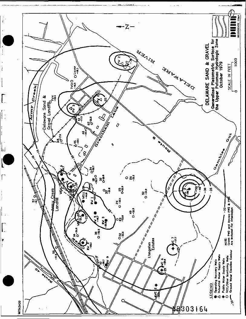
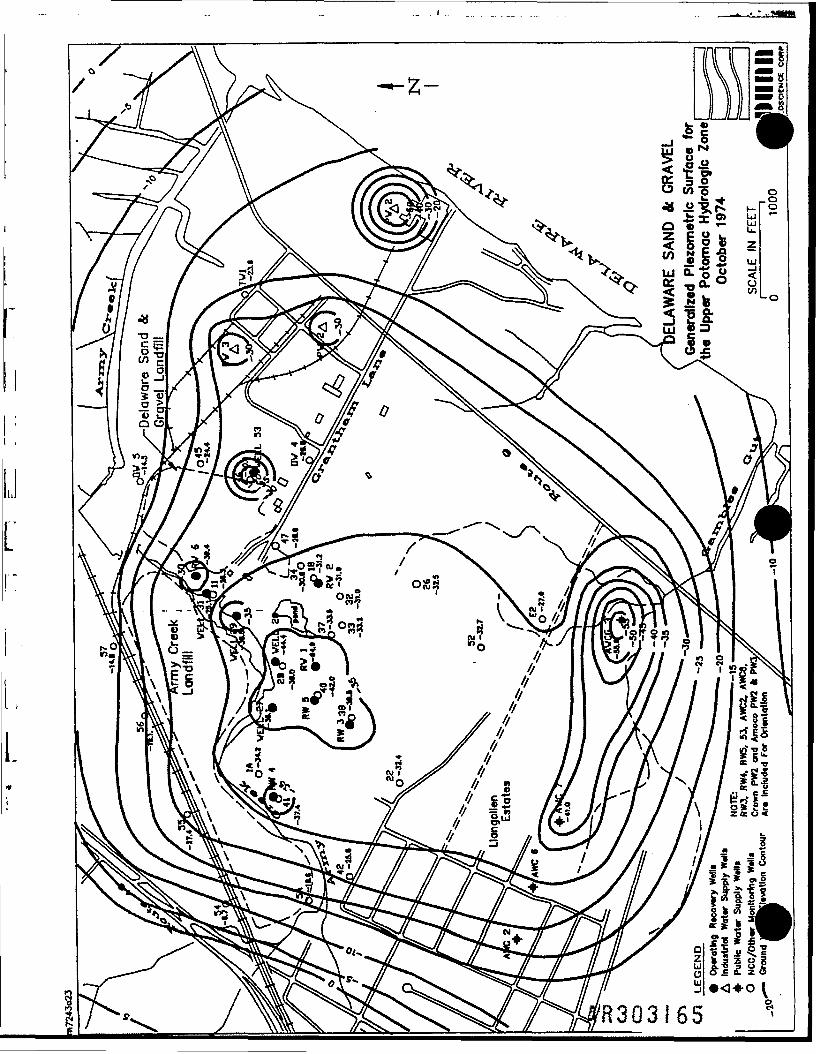
Piezometric Surface Maps
HS383I6I


•o+o R303I65 *
cE4
Water Level Tables
AR303166
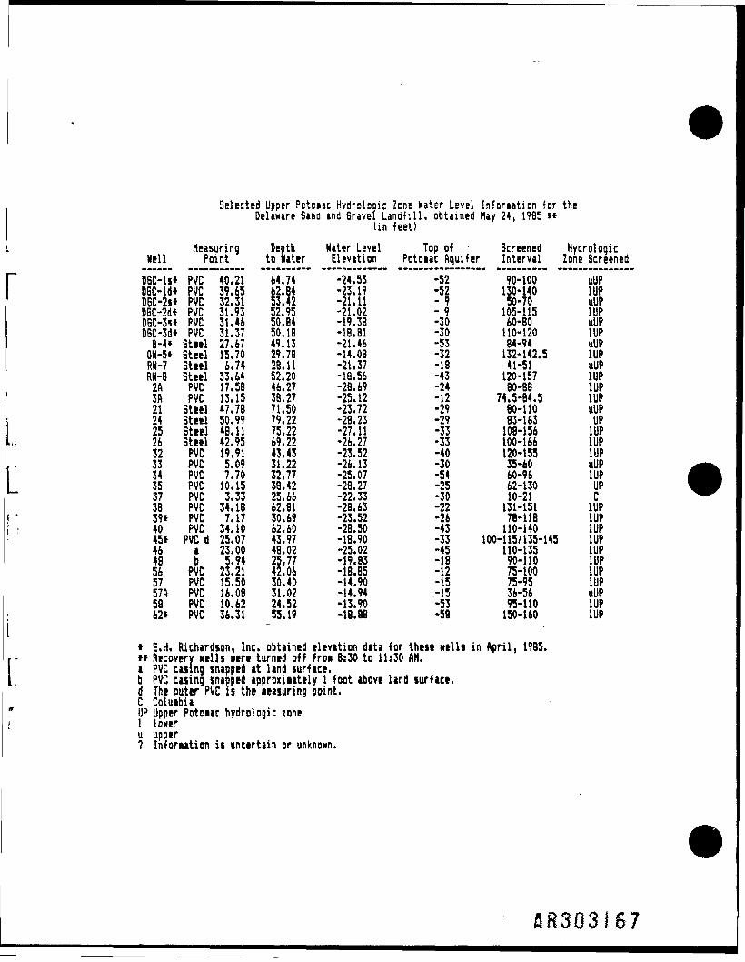
Selected Upper Potoiac Hvdroloqic Zone Hater Level Inforiaticn for theDelmre Sand and Sravel Landfill, obtained Hay 24, 1985 »«
tin feet)Measuring Depth Hater Level Top of • Screened Hydrologic
Hell Point to Niter Elevation Potoiac Aquifer Interval Zone ScreenedDBC-ll* PVC 40.21 64.74 -24.53 -52 90-100 uUPD6C-id* PVC 39.65 62.84 -23.19 -52 130-140 1UPD6C-21* PVC 32.31 53.42 -21,11 - 9 50-70 uUPD6C-2d* PVC 31.93 52.95 -21.02 - 9 105-115 1UPDEC-31* PVC 31.46 50.B4 -19.38 -30 60-80 uUPDBC-3d* PVC 31.37 50.18 -18.81 -30 110-120 IUP
B-4» Stiel 27.67 49.13 -21.46 -53 84-94 uUPOU-5* Steel 15.70 29.78 -14.08 -32 132-142.5 IUPRH-7 Steel 6.74 28.11 -21.37 -18 41-51 uUPRH-8 Steel 33.64 52.20 -18.56 -43 120-157 IUP2ft PVC 17.58 46.27 -28.69 -24 80-88 IUP3ft PVC 13.15 38.27 -25.12 -12 74.5-84.5 IUP21 Sttel 47.78 71.50 -23.72 -29 80-110 uUP24 Steel 50.99 79.22 -28.23 -29 83-163 UP25 Still 48.11 75.22 -27.11 -33 108-156 IUP26 Stetl 42.95 69.22 -26.27 -33 100-166 IUP32 PVC 19.91 43.43 -23.52 -40 120-155 IUP33 PVC 5.09 31.22 -26.13 -30 35-60 uUP34 PVC 7.70 32.77 -25.07 -54 60-96 IUP35 PVC 10.15 38.42 -28.27 -25 62-130 UP37 PVC 3.33 25.66 -22.33 -30 10-21 C38 PVC 34.18 62.81 -28.63 -22 131-151 IUP39* PVC 7.17 30.69 -23.52 -26 78-118 IUP40 PVC 34.10 62.60 -28.50 -43 110-140 IUP45* PVC d 25.07 43.97 -18.90 -33 100-115/135-145 IUP46 a 23.00 48.02 -25.02 -45 110-135 IUP48 b 5.94 25.77 -19.83 -18 90-110 IUP56 PVC 23.21 42.06 -18.85 -12 75-100 IUP57 PVC 15.50 30.40 -14.90 -15 75-95 IUP57ft PVC 16.08 31.02 -14.94 .-15 36-56 uUP58 PVC 10.62 24.52 -13.90 -53 95-110 IUP62* PVC 36.31 55.19 -18.88 -58 150-160 IUP
* E.H. Richardson, Inc. obtained elevation data for these mils in April, 1985.>* Recovery Nells wen turned off frn 8:30 to 11:30 AH.a PVC casing snapped at land surface.b PVC casing snapped approxiiately I foot above land surface.d The outer PVC is the msuring point.C ColuibiaUP Upper Potoiac hydrologic zone1 loneru upper? Information is uncertain or unknown.
-AR3Q3I67
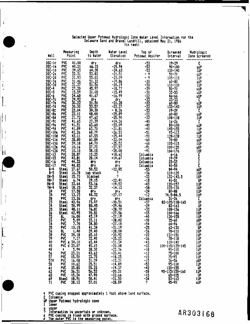
Selected Upper Potoiac Hydrologic Zone Nater Level Inforiation for theDelaware Sand and Sravel Landfill, obtained Hay 21, 1986
(in feet)Measuring Depth Nater Level Top of Screened Hydrologic
Nell Point to Nater Elevation Potoiac Aquifer Interval Zone ScreenedDBC-lc PVC 41.00 dry dry -52 19-29 CDBC-ls PVC 40.21 66.15 -25.94 -52 90-100 uUPDBC-ld PVC 39.65 64.28 -24.63 -52 130-140 IUPDBC-2s PVC 32.31 53.82 -21.51 - 9 50-70 uUP .D6C-2d PVC 31.93 55.02 -23.09 - 9 105-115 IUPD6C-3S PVC 31.46 51.32 -19.86 -30 60-80 uUP
| DBC-3d PVC 31.37 51.56 -20.19 -30 110-120 IUPDBC-4 PVC 27.20 45.97 -18.77 -39 50-70 uUPD6C-5 PVC 15.59 31.08 -15.49 -30 35-55 uUPDEC-6 PVC 24.68 41.67 -16.99 -22 46-66 uUPDBC-7c PVC 29.92 dry dry -22 23-33 CD6C-7S PVC 30.22 51.50 -21.28 -22 60-80 uUPDBC-7d PVC 30.30 53.57 -23.27 -22 133-143 IUPDBC-Bc PVC 22.04 30.30 - 8.26 -32 19-29 CDEC-85 PVC 22.11 48.00 -25.89 -32 60-80 uUPDBC-8d PVC 21.72 47.62 -25.90 -32 108-118 IUPD6C-9C PVC 41.65 27.39 +14.26 -40 16-26 CD6C-9s PVC 41.51 63.60 -22.09 -40 80-100 uUPDBC-9d PVC 41.89 63.70 -21.81 -40 145-155 IUPDBC-lOs PVC 42.26 68.79 -26.53 -51 93-113 uUP
1 DBC-lOd PVC 42.11 67.55 -25.44 -51 128-138 IUPDBC-lls PVC 38.80 60.84 -22.04 -60 70-80 uUPDBC-lld PVC 39.18 64.70 -25.52 -60 105-115 IUPDBC-12S PVC 10.16 37.73 -27.57 -91 100-120 uUPDEC-12d PVC 10.10 38.18 -28.08 -91 166-176 IUPDBC-13 PVC 28.87 10.25 +18.62 Coluibia 6-16 CDEC-15 PVC 42.81 28.14 +14.67 Coluibia 19-29 CD6C-16 PVC 44.33 dry dry Coluibia 23-33 CD6C-17 PVC 48.85 dry drv Coluibia 40-50 C8-4 Steel 27.67 50.52 -22.85 -53 84-94 uUPB-5 Steel 16.78 cap stuck ? -36 110-120 IUPON-5 Steel 15.70 blocked ? -32 132-142.5 IUPRN-7 Steel 6.74 29.15 -22.41 -18 41-51 UPRN-8 Steel 33.64 53.16 -19.52 -43 120-157 IUPTN-4 Steel 18.15 32.27 -14.12 -58 125-130 IUP2A PVC 17.58 dry dry -24 80-88 IUP
, 3ft PVC 13.15 40.32 -27.17 -12 74.5-84.5 IUP38 PVC 13.36 dry dry Coluibia 21-26 C
1 23 Steel 42.96 73.47 -30.51 -37 82-105/118-165 UP24 Steil 50.99 80.45 -29.46 -29 B3-163 UP25 Steel 48.11 76.81 -28.70 -33 108-156 IUP
i 26 Steel 42.95 70.51 -27.56 -33 100-166 IUPI 32 BL 16.00 43.19 -27.19 -40 120-155 IUP1 33 PVC 5.09 33.11 -28.02 -30 35-60 uUP
34 PVC 7.70 34.80 -27.10 -54 60-96 IUP35 PVC 10.15 41.34 -31.19 -25 62-130 UP36 BL 1.40 29.40 -28.00 -26 70-110 IUP38 PVC 34.18 65.10 -30.92 -22 131-151 IUP39 PVC 7.17 32.40 -25.23 -26 78-118 IUP40 PVC a 34.10 65.44 -31.34 -43 110-140 IUP
, 45 PVC d 25.07 45.15 -20.08 -33 100-115/135-145 IUP48 * 5.94 28.30 -22.36 -18 90-110 IUP56 PVC 23.21 43.62 -20.41 -12 75-100 IUP57 PVC 15.50 33.75 -18.25 -15 75-95 IUP57A PVC 16.08 31.39 -15.31 -15 36-56 uUP58 PVC 10.62 25.51 -14.89 -53 95-110 IUP61 PVC 35.85 55.22 -19.37 -42 120-155 UP62 PVC 36.31 56.52 -20.21 -58 95-115/150-160 IUP65 PVC 15.24 47.90 -32.66 -15 65-105 UP69 Steel 18.91 50.41 -31.50 -34 53-113 IUP71 PVC 28.12 57.01 -28.89 ? 45-90 uUP
» PVC casing snapped approximately 1 foot above land surface.C ColuibiaUP Upper Potoiac hydrologic zone1 loweru upper? Intonation is uncertain or unknown. R &a PVC casing it flush with ground surface. *
_______d The outer PVC ii the ieasurinq point.

E5
Descriptive Well Logs
L
SR3Q3I69

Reni Nell (Dc 14-21) Descriptive Logprepared by John C. Killer, DBS
interval (ft. below soil description geophysical log interpretation *ground surface)
1-1010-2020-3030-4040-5050-5757-7070-8585-130
t Trt 1 4A142-145145-159159162
160-170170-180180-185180-190190-200204
200-210210-220220-230230-240240-250250-260260-270271-279279
280-290290-300300-310310-320320-330330-340340-350350-360366
370-380380-390390-400400-410410-420420-430430-440440-450450-460460-470470-480480-490490-500500-507507-519520-530530-540531-544544-545
•ed-coarse brown sandcoarse brown sand w/gravelsate as 10-20 feetsaie as 1-10 feetsaw as 1-10 feetsaw a 1-10 feetstiff red and gray Potoiac claystiff gray clayfine-wdiin gray sand
— white sand and clay lixed starting at 135 feet ——————————white claysand, cleaniron stone layerwhite clay w/redsaw as 145-159 but men clay in itwhite clay grading into red clay (red doiinant 8 180')red clay changing to gray claysaw as above w/sandy layersdark gray claylignite and gray clay coiing up in stall ballsdark gray clay w/lignite ana sow fine sands'gritty* sand until 216' w/change to light gray claygray clay w/'grit"dark gray clay•ediui gray clayred w/gray clay — 2.5' of sand (gritty) 8 257'red and gray clayfine to wdiui gray sandgray clay w/lignitesaw gray clay w/red clayred clay doiinantred clay w/lignitered clay w/sand stringers (fine to wd sand 8 312')red clay w/fine to wo sands (thin)red clay ft/stall sandsgray and red clay w/siall sandsred clay w/grit layers — drilling very hard 8 358' —-clay to 366'sandsand w/fjuch red clayred and gray clay w/coarsi sandred clay w/gritred claygray and red clay w/wd sandsawcoarse sand w/red and gray clayred clay w/coarse sandred clayred clay w/sow gray clayred clay w/sand — men sand 8 474' — sands continue to 487'very coarse sand w/sow red clayclay w/sow sandsawsand, wdiu* w/sl. clayred clay (no saiple taken)sand and claywdiui to very coarse sand — si. clayred clay
ColuHia
—————— 57- ——————uppermost Potoiacconfining clay
—————— . 85 ———————upper Upper Potoiac—————— 1351 ——————
Upper PotDiac dividing clay— ZE ——— 145- —— I — ! —lower
Upper Potoiac1£
Middle Potoiacconfining clay
Middle Potoiac
Lower Potoiacconfining clay
—————— 430' ——————
LowerPotouc
* Geophysical logs are in the Delaware Geological Survey files.
ftR3031 70
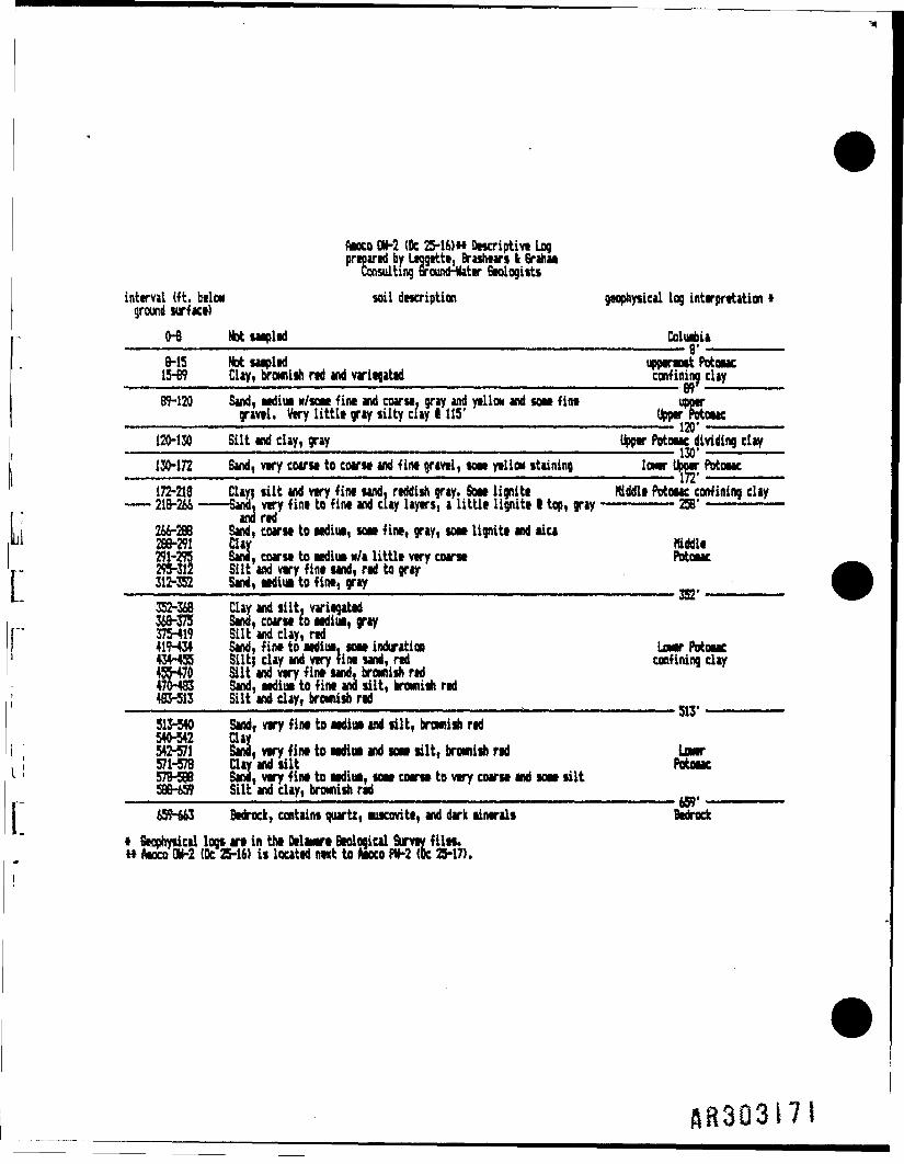
AMCO W-2 (Dc 25-16>H Dwcriptivt Log' • • gttti, Brashears k BraF
round-Hater BiologistsFHM.W Mf A till, fe ia/
prepared by Leogette, Brashears fc BrahaaConsulting Ground-?''
interval (ft. belowground surface)
0-88-1515-S989-120
120-130130-172172-218
266-298288-291291-295295-312312-352352-368368-375375-419419-434434-455455-470470-483483-513513-540540-542542-571571-578578-588
soil description
HotuMledNotsawledday, brownish red and variegatedSand, wdiui w/sow fine and coarse, gray and yellow and sow finegravel. Very little gray silty clay 8 115'
Silt and clay, graySand, very coarse to coarse and fine gravel, sow yellow stainingday) silt and very fine land, reddish gray. Sow lignite•Sand, very fine to fine and clay layers, a little lignite 8 top, gray
and redSand, coarse to wdiui, sow fine, gray, sow lignite and eicadaySand, coarse to wdita w/a little very coarseSilt and very fine sand, red to graySand, wdiui to fine, grayday and silt, variegatedSand, coarse to wdiui, graySilt and clay, redSand, fine to wdiu. tow indurationSilt; clay and very fine sand, redSilt and very fine sand, brownish redSand, wdiui to fine and silt, eromirfi ridSilt and clay, brownish redSand, vry fine to wdiui and tilt, brownish reddaySana, very fine to wdiui and tow tilt, brownish redday and tiltSani, very fine to wdiia, sow coirw to very coarse and sow tiltSilt and clay, brownish red
geophysical log interpretation *
Columbiauppermost Potoiacconfining clay
UppvPPrtouc—————— 120' ——————
Upper Moiacjiividing claylower UPJHT Potoiac
Kiddle Potoiac confining clay—————— 258* — - — • ———
HiddliPotoiac
Lower Potoiacconfining clay
—————— 513' ——————
LowerPotoiac
' • iifW* •••• ii659-663 Bedrock, contains quartz, luKovite, and dark lintralf Bedrock
t Swphytical low are in the Delaware Beological Survey files,« ftaxo W-2 (Dc 25-16) is located nwt to toco PN-2 <Dc 25-17).
SR30317I

Appendix F
Surface Geophysics
&R3Q3172

Appendix F
F.I Pertinent Site Backcrround and Conditions
The DS & G landfill consists of wastes deposited in a former sandand gravel pit. Based on reported waste disposal practices atthe site and general physiography, the landfill has been dividedinto four disposal areas. Surface geophysical methods wereapplied in three of these areas: the drum disposal area, inertwaste disposal area, and Grantham South disposal area. Theridge area was not investigated using geophysical techniques. Amap of the site showing these areas and the local topography ispresented on Plate 4.
The objectives of the surface geophysics were as follows:
o Delineate lateral extent of waste disposal andconcentrations of buried metal in the drum disposalarea;
o Delineate lateral extent of waste disposal in the inertdisposal area;
o Delineate thickness of the inert disposal area;
o Delineate lateral extent of waste disposal andconcentrations of buried metal in the Grantham Southarea;
o Delineate the lateral extent of the Uppermost Potomacclay in the drum disposal area; and,
o Delineate additional subsurface layerings or leachateplumes.
SR3Q3.73

Weather conditions during the surveys were generally good.During the first phase of the Remedial Investigation,temperatures ranged from the mid 50's to 60's. Rain on one daynecessitated implementation of special survey techniques toprevent falling behind schedule. However, the rain did notimpair the quality of the geophysical data. During the secondphase of surface geophysical work, the weather was seasonablycold, partly sunny, and windy. Light showers and snow flurriesoccurred on one afternoon. Overall, weather conditions wereacceptable for the geophysical methods employed in thisinvestigation.
Drum Disposal Area
Available information indicates that numerous steel drums wereburied and stored at the ground surface in the far northern partof the landfill. Approximately 500-600 exposed, intact ordeteriorating drums, some partly buried, were removed from thisarea prior to the RI/FS, but an unknown quantity of additionaldrums were left buried. The vertical extent of these burieddrums is uncertain but an estimate of 40 feet has beenpreviously postulated.
Prior to the initiation of the geophysical field work, it wasproposed that additional concentrations of buried drums couldalso be present in the relatively low and level grassy fieldimmediately to the south and west of the known drum disposalarea. As a result, the geophysical survey was extended wellbeyond the inferred boundary of known buried drums and into thisfield.
ftR3Q3l7l*

Evidence for the previous drum removal operation was readilyapparent during the geophysical surveys. Sparse groundvegetative cover, scattered fragments of drum lids and sealrings, rutty disturbed ground and gravel-paved access and workareas suggested the general extent of former drum removalactivities.
Field conditions in the drum disposal and adjacent areas weregenerally favorable for geophysical field work. Unfortunately,a metal fence and railroad track at the northern end of the sitecreated a band of electromagnetic interference that locally mayhave masked terrain conductivity and magnetometer anomaliescaused by buried steel drums. This effect and spuriousanomalies caused by scattered surface metal and a steelmonitoring well casing (B-l) were evaluated and taken intoaccount in the data interpretation.
Inert Disposal Area
The inert disposal area in the southern part of the landfill wasreportedly filled with cork dust, fiber trimmings, cardboard,wood, tires, possibly hazardous materials and other industrialwaste. At closure, the fill was covered with sandy materialfrom the adjacent quarry.
At the time of the geophysical surveys, the central part of thisarea was characterized by a profuse scattering of surface debrisincluding abandoned cars, school buses, appliances, furniture,and other metallic and non-metallic junk. Physical andgeophysical interference caused by the debris locally preventedmeaningful terrain conductivity and magnetic measurements.Areas not covered with junk were commonly characterized by densevegetation including thick tall grass, waist-high brush, andpricker bushes. Steep slopes formed parts of the western,northern, and eastern boundaries. Seismic refractionmeasurements indicated highly heterogeneous fill with poorseismic transmission characteristics.
ftft303175

Field conditions were generally unfavorable for geophysics inthe inert landfill because of the interference, pooraccessibility, and extremely heterogeneous subsurfaceconditions. As a result, for the sake of expediency, the extentof geophysical survey was limited in the inert landfill anddeferred to those areas where the most meaningful data could becollected in the shortest time.
Grantham South Area
The disposal area located immediately south of Grantham Lane wasidentified during the Phase I field activities of the RemedialInvestigation. As such, the scope of the Phase II fieldactivities was set up to include surface geophysics and a soilboring in this area.
Field observations indicate that the Grantham Lane South areacontains industrial wastes. Scattered empty drums and powderedchemical residuals have been observed. Unlike the main inertarea north of Grantham Lane, this area is not covered withdiscarded appliances, vehicles, and other large metallic junkwhich prevent meaningful EM and magnetic measurements.
Field conditions in the Grantham South area were generallyfavorable for geophysical field work. An overhead electricalpower line and a chain-link fence borders the northern edge ofth© Grantham Lane South area. These objects represent sourcesof local interference for the geophysical methods employed. Thepossible effects of these features and scattered surface trashwere taken into account in the data interpretation.
HR3Q3I76
F.2 Description of Geophysical Methods
This section describes the geophysical equipment used in thestudy including general principles, applications, limitationsand equipment.
Terrain Conductivity (TO Profiling
' Terrain conductivity profiling is a non-destructiveelectromagnetic induction exploration technique. Subsurfaceconductivity is measured by using a transmitter coil to createan electromagnetic field in the earth while simultaneouslymeasuring changes in the field through a receiving antennacoil. Conductivity is measured as millimhos per meter(mmhos/m).
TC profiling is a rapid and effective reconnaissance method fordetermining lateral variations in terrain conductivity ofsubsurface materials within various depths of exploration.Terrain conductivity instruments are not designed for detailedexploration of the vertical variations of conductivity withdepth. Such vertical variations are better explored usingconventional resistivity sounding techniques.
The depth of a TC exploration depends upon the instrument used,the spacing and configuration of the transmitting and receivingdipoles and the transmitting frequency. The commerciallyavailable TC instruments have fixed or limited dipole spacingoptions and operate in the 0.4 to 9.8 kilohertz range;therefore, the ability to investigate to different depths islimited.
A Geonics EM-31 and a Geonics EM-34 were two commerciallyavailable TC instruments used in this study. The Geonics EM-31unit employed during the study has a fixed dipole spacing (i.e.,
•W303I77

distance between transmitter and receiver) and an effectivemaximum depth of investigation of approximately 20 feet. Theeffective depth of investigation for the Geonics EM-34 unitemployed is dependent upon the dipole spacing and dipoleorientation. The spacings utilized during the survey were asfollows:
Depth of Investigation Depth of InvestigationDipole Spacing (Vertical Dipole) (Horizontal Dipole)
10m 15m ( 50 feet) 7.5m ( 25 feet)20m 30m (100 feet) 15.0m ( 50 feet)40m 60m (200 feet) 30.0m (100 feet)
Terrain conductivity measurements respond to properties thataffect the ability of the subsurface materials to transmit aninduced electrical current. The properties include the type ofsoil or rock, porosity, degree of saturation, and specificconductance (total dissolved solids) of contained fluids. Thus,variations in moisture content, soil thickness, ionicgroundwater contamination, and relative proportions of gravel,sand, and clay will affect terrain conductivity measurement.
Determining which factors are responsible for observedconductivity variations generally requires additionalinformation from borings, well logs, or other data sources. ingeneral, conductivities are higher in the presence of soils thatare clayier, wetter, thicker, or contaminated with inorganicchemicals, and are lower for sand, dry or thin soils, orgroundwater not significantly contaminated by inorganics orelectrolyte-rich solutions.
HR3Q3I78

Highly conductive, nearby cultural features including overheadpower lines, steel fences, buildings, railroad tracks, culverts,buried pipes, and large quantities of metallic objects willadversely affect the readings, but minor amounts of scatteredmetallic surface debris are generally not troublesome. However,the signal response of the EM-31 is somewhat limited, and forvery high conductivities, the indicated values may roll over andbecome lower instead of higher. Conductivities greater thanapproximately 1,000 mmhos/m, which are common for measurementsnear metallic cultural features such as those listed above, willresult in zero or negative values. The presence of nearbyconductors may also cause the TC values to be unstable andhighly sensitive to the directional orientation of the coils.Abrupt lateral changes in conductivity may also result in zeroor negative values.
Landfill areas are usually, but not always, more conductive thanbackground values and display a high variability of TC values.Conductive fill includes metallic-rich waste and watercontaining a high salt or electrolyte content such as ash orsanitary waters, respectively. Zero or unstable values may beindicative of buried metal such as drums. Coarse, inert wastesuch as glass, masonry, rubble, bricks, wood, and cinderswithout metallics are examples of wastes usually exhibiting lowconductivity. Organic contaminants have low conductivities andare difficult to detect using the EM method unless they occurwith the more highly conductive electrolyte-rich contaminants.
The Geonics EM-31 was used in its normal vertical dipoleconfiguration. In this configuration, the EM-31 is relativelyinsensitive to small surface metallic trash, but still isadequately sensitive to detect areas of buried metal drums.
i83Q3l7S
A Geonics EM-34 terrain conductivity meter was used to performfour traverses in the northern part of the landfill area nearthe drum disposal area. A 20-meter intercoil spacing was usedwith the dipoles in both vertical and horizontal orientations.The 20-meter intercoil spacing resulted in an optimum effectivedepth of exploration to investigate the nature of the UpperPotomac confining clay which occurs at depths in excess of 30feet.
Magnetometer Surveying
Magnetometer surveying measures the spatial variations in theearth's magnetic field intensity. Perturbations in the magneticfield may be caused by local concentrations of strongly orweakly magnetic materials in contrast with each other and theambient medium. Iron and most steel, such as in drums forexample, are ferromagnetic and contrast sharply with soil, whichis usually very weakly magnetic. This contrast can result in ameasurable positive or negative disturbance, i.e., anomaly, inthe ambient magnetic field.
Magnetic anomalies can be highly variable in amplitude andshape, even for simple sources. The causes of this complexityinclude the strength and direction of the earth's magneticfield, the relative direction and intensity of the permanent andinduced magnetic moments in the source, the shape and size(volume and mass) of the body and its depth and configuration.Anomalies caused by accumulations of ferromagnetic objects suchas steel drums are especially complex because they commonlyportray the combined magnetic effects of several discretesources, they have variable magnetic properties, they can be indifferent states of deterioration (iron rust is not particularlymagnetic), or they can manifest possible demagnetization effectswhereby the anomaly is much smaller than would be normallyexpected. Furthermore, there are an infinite number of possiblesources that could provide a given anomaly. As a result,quantitative interpretations are generally not feasible. This
HR303I8

report is, therefore, directed towards a qualitativeunderstanding of the observed anomalies. Magnetic intensity ismeasured in gammas (also called nanoteslas).
A Geo-Metrics G856 portable proton precession magnetometer wasused for the magnetometer survey. The sensor was mounted on thetop of an 8-foot high aluminum staff, held vertically by asecond field person at some distance from the console. In thisconfiguration, the magnetometer is relatively insensitive tosmall surface ferrous trash, but remains adequately sensitive todetect buried steel drums. The magnetometer operates bymeasuring the frequency of protons precessing or oscillatingabout the ambient magnetic field vector after an internal,temporary applied, polarizing force is removed. The precessionfrequency is proportional to the magnetic field intensity, whichis the measured parameter.
Seismic Refraction Surveying
The seismic refraction method is based on the principle ofmeasuring the velocity of seismic waves generated through thesubsurface. Different subsurface layers are detected by virtueof their ability to transmit seismic waves at contrastingvelocities, commonly expressed in units of feet or meters persecond.
Velocity measurements are made by generating a seismic impulsein the ground at a "shotpoint" and timing how long it takes thecompression or P-waves generated by this impulse to arrive at anumber of sensors (geophones) spaced at measured distanceintervals from the shotpoint along a linear traverse or spread.Sometimes it is difficult to determine the initial arrival timeof the impulse, especially if the soil layers greatly attenuatethe signal or if the background noise level masks the signal.
18383181
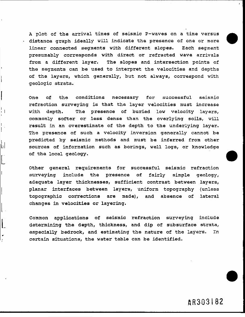
A plot of the arrival times of seismic P-waves on a time versusdistance graph ideally will indicate the presence of one or morelinear connected segments with different slopes. Each segmentpresumably corresponds with direct or refracted wave arrivalsfrom a different layer. The slopes and intersection points ofthe segments can be used to interpret the velocities and depthsof the layers, which generally, but not always, correspond withgeologic strata.
One of the conditions necessary for successful seismicrefraction surveying is that the layer velocities must increasewith depth. The presence of buried low velocity layers,commonly softer or less dense than the overlying soils, willresult in an overestimate of the depth to the underlying layer.The presence of such a velocity inversion generally cannot bepredicted by seismic methods and must be inferred from othersources of information such as borings, well logs, or knowledgeof the local geology.
Other general requirements for successful seismic refractionsurveying include the presence of fairly simple geology,adequate layer thicknesses, sufficient contrast between layers,planar interfaces between layers, uniform topography (unlesstopographic corrections are made), and absence of lateralchanges in velocities or layering.
Common applications of seismic refraction surveying includedetermining the depth, thickness, and dip of subsurface strata,especially bedrock, and estimating the nature of the layers. Incertain situations, the water table can be identified.
SR3Q3182

Seismic refraction surveying is an indirect method of- identifying subsurface conditions. Reliability ofinterpretations is significantly improved by correlating theseismic information with borings, well data, or other sources ofsubsurface information.
A soil test Model MD-9, single channel, signal enhancementseismograph was used with a tamper/hammer energy source. Thisinstrument and energy source combination has a depth detectioncapability on the order of 30 to 60 feet depending upon therelative seismic velocities and background noise levels.
Resistivity Soundings
The objective of resistivity soundings is to measure thevertical (depth) variation of apparent earth resistivity. Theoperation principle of the resistivity method is dependent onearth materials being conductors of electricity, generally inproportion to their content of dissolved salts and water. Thus,different earth materials may have contrasting resistivity
I values.i
; Electrical resistivity studies were conducted using a BisonInstruments Model 2350 earth resistivity meter. The fieldtechniques consisted of laying out and inserting into the ground
LL four co-linear electrodes wired to a resistivity meter. Acurrent is passed through the two end electrodes and the
| resulting potential difference between the two inner electrodesis measured. Wider electrode spacings are used to penetrate to
r
I greater depths. The Wenner array geometry, which consists ofequally spaced electrodes, was used for this study. Theequation used to calculate apparent resistivity from the currentand potential data depends upon the geometry of the electrodearray. Resulting apparent resistivities are expressed in unitsof ohm-meters (this study) or ohm-feet and are plotted onlog-log graph paper as a function of electrode spacing expressedin feet.
RB303183

For this study, the resistivity sounding data were interpretedusing the Barnes Layer method. The Barnes Layer method is afast, cost-effective, semi-empirical method which assumes, as afirst approximation, the depth of investigation is equal to theelectrode spacing. Resistivity soundings and terrainconductivity surveying typically complement each other.
Difficulties applying this method will occur if the ground istoo hard to insert electrodes or too dry to conduct sufficientcurrent. Additional difficulties in interpretation will occurif any of the following conditions are present: significantlateral variations in resistivity, complex layering, gradationalcontacts, irregular topography, and large rock dips. Layersmust be adequately thick and have sufficient contrast withadjacent layers to be detectable. Buried or surface conductors,especially those parallel to the array, may cause interferenceand prevent reliable measurement.
F.3 Site-Specific Methodology and Results
The four geophysical techniques applied to achieve the projectobjectives were terrain conductivity profiling, magnetometersurveying, seismic refraction and resistivity sounding. Thetechniques were applied to specific tasks based on their provencapability for producing meaningful results under similarconditions. A description of the site specific methodology foreach technique, the rationale for utilizing it, and the resultsare provided in this section of the report. The objectivesaddressed are:
o location of buried metal in the drum disposal area;o landfill boundaries in the inert disposal area;o landfill thickness in the inert disposal area;o location of buried metal and landfill boundaries in the
Grantham South area; and,o the nature of the Upper Potomac confining clay.
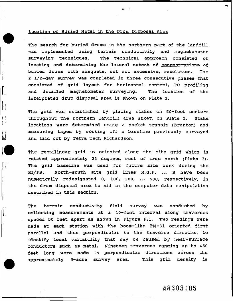
Location of Buried Metal in the Drum Disposal Area
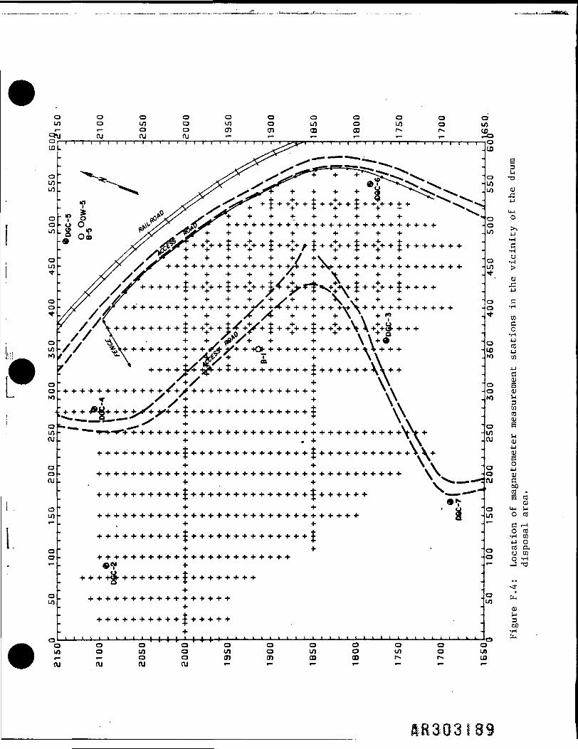
The search for buried drums in the northern part of the landfillwas implemented using terrain conductivity and magnetometersurveying techniques. The technical approach consisted oflocating and determining the lateral extent of concentrations ofburied drums with adequate, but not excessive, resolution. The2 1/2-day survey was completed in three consecutive phases thatconsisted of grid layout for horizontal control, TC profilingand detailed magnetometer surveying. The location of theinterpreted drum disposal area is shown on Plate 3.
The grid was established by placing stakes on 50-foot centersthroughout the northern landfill area shown on Plate 3. Stakelocations were determined using a pocket transit (Brunton) andmeasuring tapes by working off a baseline previously surveyedand laid out by Tetra Tech Richardson.
The rectilinear grid is oriented along the site grid which isrotated approximately 23 degrees west of true north (Plate 3).The grid baseline was used for future site work during theRI/FS. North-south site grid lines H,G,F, ... B have beennumerically redesignated 0, 100, 200, ... 600, respectively, inthe drum disposal area to aid in the computer data manipulationdescribed in this section.
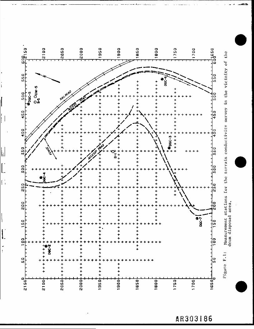
The terrain conductivity field survey was conducted bycollecting measurements at a 10-foot interval along traversesspaced 50 feet apart as shown in Figure F.I. Two readings weremade at each station with the boom-like EM-31 oriented firstparallel and then perpendicular to the traverse direction toidentify local variability that may be caused by near-surfaceconductors such as metal. Nineteen traverses ranging up to 450feet long were made in perpendicular directions across theapproximately 5-acre survey area. This grid density is
A83G3185
V
.. i r**:*.,.,:** : *:* **
O J O J
luo
c•HO•H
a)'>t-4
W
4-1•H
o3•aco
•HCOr-l0)
IV) 4J
01rC
cnco4-1 CU
. t I
4-1 COtn
r—I4J COC wnj OB a.3 tn
ftR303i86

['
at cu
BR303I87
mo
ra01
raU)oe-tn
ED
0)
u-iO
01 .a >—.C tn0) rJrJ 30) O
14-J 4-1<« C•H O-a u>> E4J ~•H O> £•u Eu3 inT3 CM
O T3O Crac•H *tO OrJ Mot ^H m
00
•4-4-4-4-4-4-4-4-4-4-4' 4 - 4 + 4-4-4-4-4.4-4-4-4-4-4-4-
»4-4-4-4-4-4-4-4-4-4-4-4'4-4-4-4-4-4'4-4-4-4'4-4-4-4-4-4'4-4-4-4'W4>
4- 4- \ \•f + 4-4-4> + 4>4-4>4-4> + 4-4-4- + 4-4-4-4-4-4-4-4-4-4-4-4-4-4-4-4' + 4-4-4- \ \
IB303I89
sufficient for locating the large concentrations of buried drumsknown to occur in the area and was judged cost-effectiveconsidering the purpose of the project. Before the survey wasinitiated a preliminary traverse, Terrain Conductivity ProfileNo. 1 was completed to verify the ability of the EM-31 to detectburied drums at the site. The results of this traverse,discussed in the following section, Landfill Boundaries in theInert Disposal Area, clearly demonstrate that the drum disposalarea produces a significant anomaly.
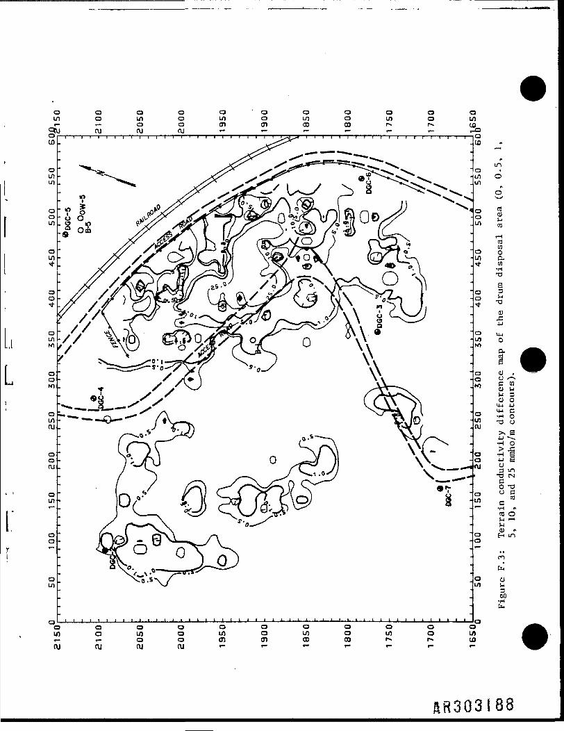
For preliminary in-field evaluation, the EM-31 data were plottedand hand contoured. To facilitate final interpretation, thedata were computer contoured with a variable contour interval toemphasize anomalies. The contour map is shown in Figure F.2.
A plot of the absolute value of the difference of the two EM-31readings at each station was also made to emphasize subtleanomalies (Figure F.3). Delineation of buried drum areas wasbased on interpreting the two individual EM-31 contour plots andcomparing them with each other and with the magnetometer data.Areas of anomalously high, low, or variable terrain conductivitywere interpreted to be probable concentrations of buried metal,presumably buried drums, less than 15 feet deep.
The magnetometer field survey was conducted by collectingmeasurements at a 10-foot interval along 33 traverses spaced 25to 50 feet apart as shown in Figure F.4. The closer 25-foottraverse spacing was employed in the vicinity of the buried drumdisposal area to provide greater resolution than the coarser50-foot spacing would allow. These grid spacings were selectedas optimum on© considering the time and budgetary constraints.
SR303I-90
Although the readings were stored in the instruments digitalmemory for subsequent processing in the office, fieldmeasurements were also recorded manually for plotting at thefield site. This enabled preliminary interpretations andadjustments in field methods as necessary. For finalinterpretation, the data were computer contoured with a variablecontour interval. Because of the extreme variability in themagnitude of the measured values, the site was subdivided intotwo areas and each area was contoured with a different contourinterval. These contour maps are shown in Figures F.5 and F.6.Data smoothing, other than contouring, and correction for thetemporal variations (drift) in the earth's magnetic field werejudged not necessary due to magnitude of the anomalies, thoughoccasional field checks of drift were made and found to beacceptably low.
Interpretation was done in a similar manner to the EM-31 datareduction. Locations of high and/or low magnetic intensity wereinterpreted as probable areas of buried metal. The relativemagnitude and shape of anomalies were used to estimate relativequantities, thicknesses and depths of metal. Unlike the EM-31,which has limited depth detection, the magnetometer istheoretically not limited in depth of investigation.
Landfill Boundaries in the Inert Disposal Area
Landfill boundaries were investigated with geophysicaltechniques to confirm that they could be deduced fromtopographic or other field evidence. Approximately 1 day offield work was expended in the effort during the first phase ofwork by a two-man crew using terrain conductivity and magneticsurveying. An additional day of field work was expended duringthe second phase of work to detail the western boundary of theinert disposal area.
ftB303!9!

ra60
ooo
racuu •ra /•••>•aiH O)« r-lcn a.o a.CL, -Hcn 4-i•H tnTJE cu3 d(
)-i C
curC «4-1 01
V-iu-t coO
r-l
ra tnS oVI CO3 i-lO T34-Jc eO 3O M
cn rac >0) rJ
C 4-*•H C
•rlU•H rJ4J 3CU Oa 4->60 Cra o
mbcu
so•H
flB303l92
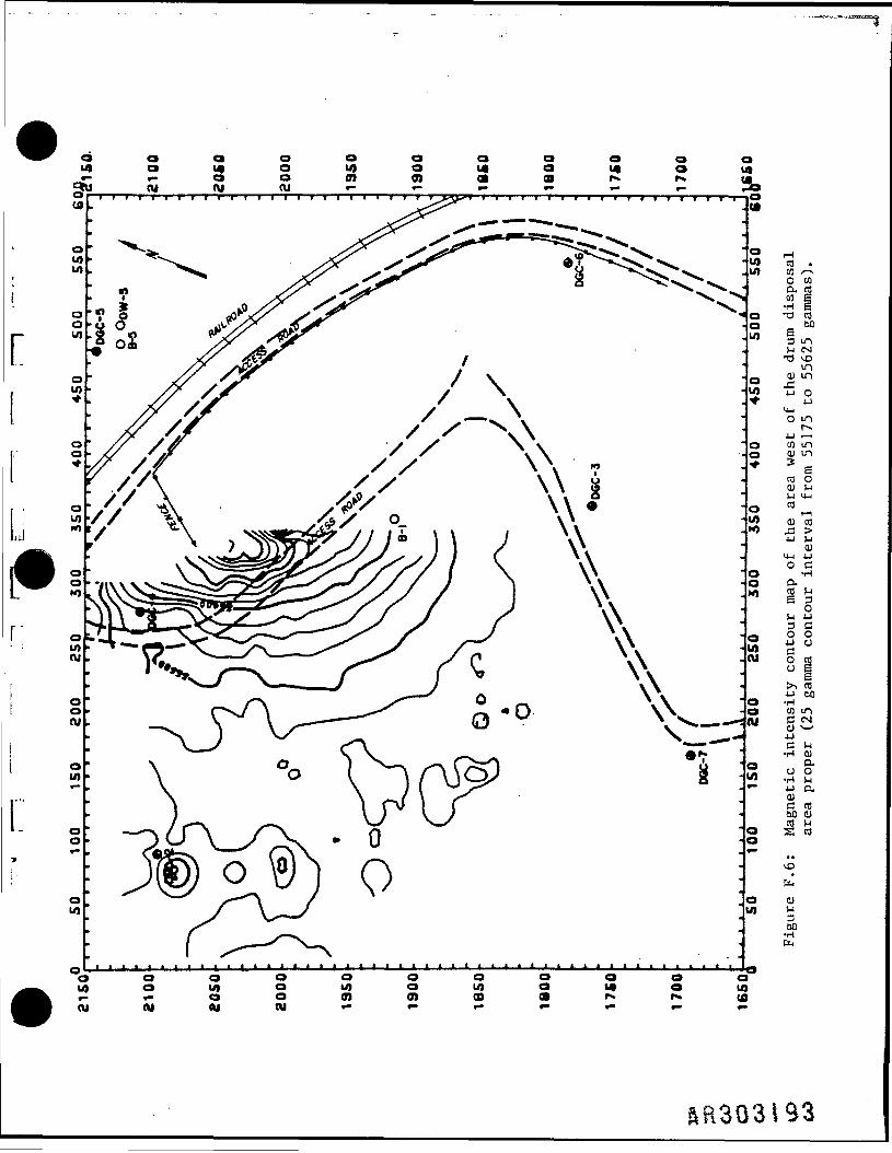
CO *CO /-No cnCu COcn g-o raoo3 mrJ CMT) Om01 m4-1 O
4JU-lo m
tn mo> m9 ECO O01 >UVJ 14-4ra
rHcu rarC >4-J 1-4
0)14-1 4-JO C
•Ha.ra Mo
V4 4J3 co o4J CJ
§ ra04J 60•Hcn mC CM01 4-1C M•H CUaa o•rl 1-44-1 a.cuc ra60 0)
Q)t-i
60
IR303I93
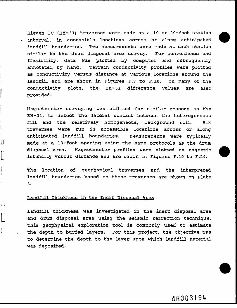
Eleven TC (EM-31) traverses were made at a 10 or 20-foot stationinterval, in accessible locations across or along anticipatedlandfill boundaries. Two measurements were made at each stationsimilar to the drum disposal area survey. For convenience andflexibility, data was plotted by computer and subsequentlyannotated by hand. Terrain conductivity profiles were plottedas conductivity versus distance at various locations around thelandfill and are shown in Figures F.7 to F.18. On many of theconductivity plots, the EM-31 difference values are alsoprovided.
Magnetometer surveying was utilized for similar reasons as theEM-31, to detect the lateral contact between the heterogeneousfill and the relatively homogeneous, background soil. Sixtraverses were run in accessible locations across or alonganticipated landfill boundaries. Measurements were typicallymade at a 10-foot spacing using the same protocols as the drumdisposal area. Magnetometer profiles were plotted as magneticintensity versus distance and are shown in Figures F.19 to F.24.
The location of geophysical traverses and the interpretedlandfill boundaries based on these traverses are shown on Plate3.
Landfill Thickness in the Inert Disposal Area
Landfill thickness was investigated in the inert disposal areaand drum disposal area using the seismic refraction technique.This geophysical exploration tool is commonly used to estimatethe depth to buried layers. For this project, the objective wasto determine the depth to the layer upon which landfill materialwas deposited.

uinjp pcpojjoo uioji »|OH
jo
E
O),C
o4J
a•H
cu1-4.•Hor-lD.
3 ra"d 01C M
•H cnra oJ-t CUM cn0) -HH T3
01r-4
60
UJ9
UIOJJVJ.
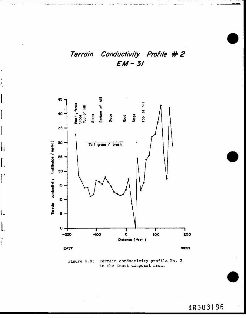
Terrain Conductivity Profile it 2EM-
45-
40-
35-
^ 3O-
^25-
=£20-
.&| 15-
10-c•oI 5-
I I I I-200 -KX> 0 100 200
Distano* ( fMt )
EAST WEST
Figure F.8: Terrain conductivity profile No. 2in the inert disposal area.
ft«303!96

Terrain Conductivity Profile & 3EM- 31
60 -
•—•—• TC Dlffer«nc«
O-IOO not totool* due to
-_.___ J0 100 200 300
Distance ( f««t )
EAST WEST
Figure F.9: Terrain conductivity profileNo. 3 in the inert disposalarea.
IR303197
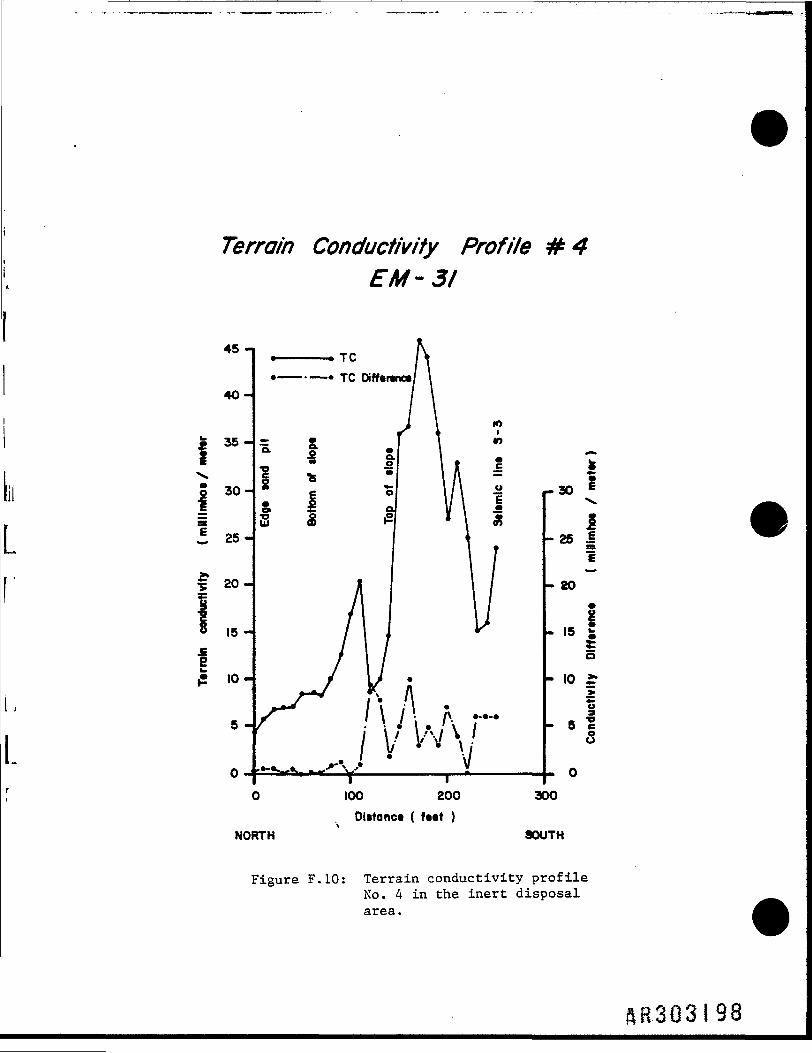
Terrain Conductivity ProfileEM-31
45 -i
40-
35 -ft 3. X I fc
30-1
I 25
0 - -
-30 v.
- 25 |1
h 2O
15 H/ I I
5
10 H / V : •"lo *^r^ i- A- / \ / \ i\ .....O *>11
Sh 6 ?
3
I T0 100 200 300
Ditto net ( f««t )NORTH * SOUTH
Figure F.10: Terrain conductivity profileNo. 4 in the inert disposalarea.
ftR.303198

IE
ou
Terrain Conductivity ProfileEM-31
- 50
0 KDO 200 30O
Distance ( f«»t )
NORTH SOUTH
Figure F.ll: Terrain conductivity profileNo. 5 in the inert disposalarea.
ftR393!99

*
= 10 H1
i
Terrain Conductivity Profile it 6EM-31
i " *O- O e
I i iI
I T T I0 100 200 300
Dfctonc* ( fttt )
WEST EAST
Figure F.12: Terrain conductivity profile No. 6in the inert disposal area.
( ..•(•MM / tOMUiiiijuu ) eoucjtuip <|iAi4onpuoo
i _____ i ___ i ___ i
00 +« 2X
L
[
UJ
C
k 8o
cuU-4OS-la.
§ *
bl
4J ra•H 0)
•H raS *->m CJr-l5 3 ra
8" T3 CO0 O
01 O Cua co
ra 4-1rJ CUcu cH i-l
0)M360•HPw

I
i:
( J«4»ui / •xxj.uijiuui ) XjtAdonpuoo
8 E
- 8
I
i S
raw
cuc
- ? >HO £2 •£ ooEe o
•Hu-iOJ-i
•H
O
Pt4
0>3

O)
JOO P9U.SOUJS P|0 0| 4»U J /002.I "(D4S
MJ«ADJ4 jo 4u;od BUIUJPJ.D8JD
L r§7WMJ3 «O|
0*4
D»JO 4J«ui ' >|onJ4 motto *0|
1 5. £
pooj
o
S S 8 S ( o 9 « o
U|OJJ»X
01c
cur-i•HU-lOCU>,
•H4JO3 ra•a 01C rJo rao
rHc ra•H COra ou cur-4 CQcu -HE—I rrj
60•rl
ft.R303203
Terrain Conductivity Profile it IOEM- 31
15 -i
= 10
5 -
- TC•——• — • TC Difftrtnct 2
L. E
8- 10 |
i
- 5
§u
0 KX) 200 300Distance ( f««t )
EAST WEST
Figure F.16: Terrain conductivity profileNo. 10 in the inert disposalarea.
R830320U
I
[
Terrain Conductivity Profile # 11EM-31
I40-|
130-•————• TC
*— ———x TC Diff«r«nc8
0 100 200 300 400
Distance (f««t)
SOUTHWEST NORTHEAST
Figure F.17: Terrain conductivity profile No. 11 in theinert disposal area.
&R3032Q5
Terrain Conductivity Profile #12EM-31
I4O -i
ISO -
120 -
70 H
1 60
I 50 -
40 -
30 -
2O -
(0 -
TC
x————* TC Difference
110 H
100 -
-. ^ "
j --L II I•? U I I ^ «.» V "^ ^ 4^
a
200 30O 400 5OO
Distance (feet)SOUTHEAST NORTHWEST
Figure F.18: Terrain conductivity profile No. 12 inthe inert disposal area. -RR303206
Magnetic Traverse # IG 856
57000
56000•
oa*"" 55OOO
S
* 54000
53OOO0 100 200 300 400
Distance ( feet )
EAST WEST
Figure F.19: Magnetometer profile No. 1 in theinert disposal area.
&R303207
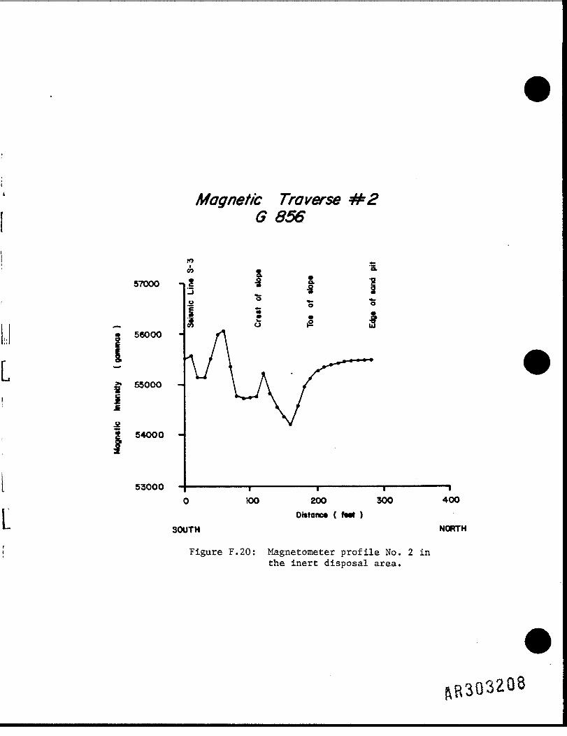
Magnetic Traverse it2G 856
L
57000
56000
55000
54000 -
53000 -f——-———----- f0 KX> 200 300 40O
Distance ( feet )SOUTH NORTH
Figure F.20: Magnetometer profile No. 2 inthe inert disposal area.
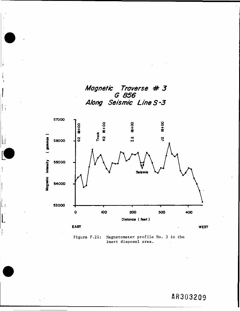
Magnetic Traverse it 3G 856
Along Seismic Line S-3
57OOO
56000
x 55000
.2£ 54000
L! 53000
0 100 200 300 400Distance (feet)
EAST . WEST
Figure F.21: Magnetometer profile No. 3 in theinert disposal area.
A83032Q9

Magnetic Traverse it 4G 856
56000
1 55500
55000
,s
5450O
54000400 50O 6OO 700 800
Distance (feet)
SOUTH NORTH
Figure F.22: Magnetometer profile No. 4 in theinert disposal area.
RR303210
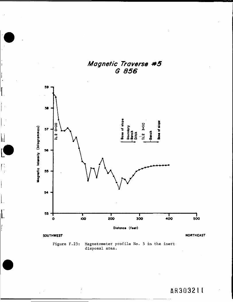
Magnetic TraverseG 856
59 -
5t -
S 57^EEe
"-" 56 -**'•
n i?54 -
53
a.o o"
« \ ? IM» «y S ?9
• 3 c o M e <Z
100 200 300 400 50O
Distance (feet)
SOUTHWEST NORTHEAST
Figure F.23: Magnetometer profile No. 5 in the inertdisposal area.
&R3G321i

Magnetic Traverse it 6G 856
59 -
58 -
is 55 —
54 -
53
8 Ie -g
S•*•CVJ
w »"
_l ffl GO Co
57 -I ______L
56 -
vi i i i i100 200 300 400 5OO
SOUTHEAST OW~ (fc"» NORTHWEST
Figure F.24: Magnetometer profile No. 6 in the inertdisposal area.
AR-303212

Three seismic lines composed of seismic refraction spreads,having a combined length of 830 feet were completed in one day.Seismic line 1, which consisted of seismic spreads 1, 2 and 3,and seismic line 2, which consisted of spread 4, were located inthe general vicinity of the drum disposal area while seismicline 3, which consisted of spreads 5 and 6 was located in theinert landfill. Progress was slower than expected because ofthe poor signal to noise ratio that required many hammer impactsto produce acceptable readings.
Each seismic spread was completed by systematically incrementingthe geophone to hammer distance by 10 feet until the measuredsignal to noise ratio degraded and became too low to use. Aftercompletion, the spread was performed in the reverse direction toresolve potentially dipping layers. The time-distance graphswere plotted in the field and monitored as the survey progressedto identify and recheck potentially spurious data. The dataplots were analyzed in the office and interpreted.
Location of Buried Metal and Landfill Boundaries in the GranthamSouth Area
The search for concentrations of buried metal and delineation ofthe landfill boundaries in the Grantham South area wasimplemented using terrain conductivity (EM-31) and magnetometersurveying techniques. The 2 1/2-day survey performed during thesecond phase of the Remedial Investigation was completed inthree consecutive phases that consisted of grid layout, TCprofiling, and magnetometer surveying.
Prior to the establishment of the grid, two perpendicularbaselines were installed using a tape and pocket transit(Brunton). Preliminary geophysical surveys were performed alongthese baselines and incorporated into data obtainedsubsequently. A grid was established with wooden stakes placed
RR303-213
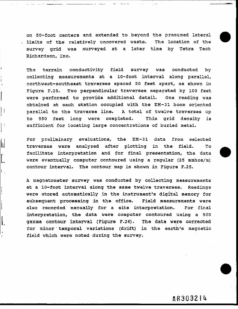
on 50-foot centers and extended to beyond the presumed laterallimits of the relatively uncovered waste. The location of thesurvey grid was surveyed at a later time by Tetra TechRichardson, Inc.
The terrain conductivity field survey was conducted bycollecting measurements at a 10-foot interval along parallel,northwest-south east traverses spaced 50 feet apart, as shown inFigure F.25. Two perpendicular traverses separated by 100 feetwere performed to provide additional detail. One reading wasobtained at each station occupied with the EM-31 boom orientedparallel to the traverse line. A total of twelve traverses upto 550 feet long were completed. This grid density issufficient for locating large concentrations of buried metal.
For preliminary evaluations, the EM-31 data from selectedtraverses were analyzed after plotting in the field. Tofacilitate interpretation and for final presentation, the datawere eventually computer contoured using a regular (25 mmhos/m)contour interval. The contour map is shown in Figure F.25.
A magnetometer survey was conducted by collecting measurementsat a 10-foot interval along the same twelve traverses. Readingswere stored automatically in the instrument's digital memory forsubsequent processing in the office. Field measurements werealso recorded manually for a site interpretation. For finalinterpretation, the data were computer contoured using a 500gamma contour interval (Figure F.26). The data were correctedfor minor ' temporal variations (drift) in the earth's magneticfield which were noted during the survey.
AR3032U
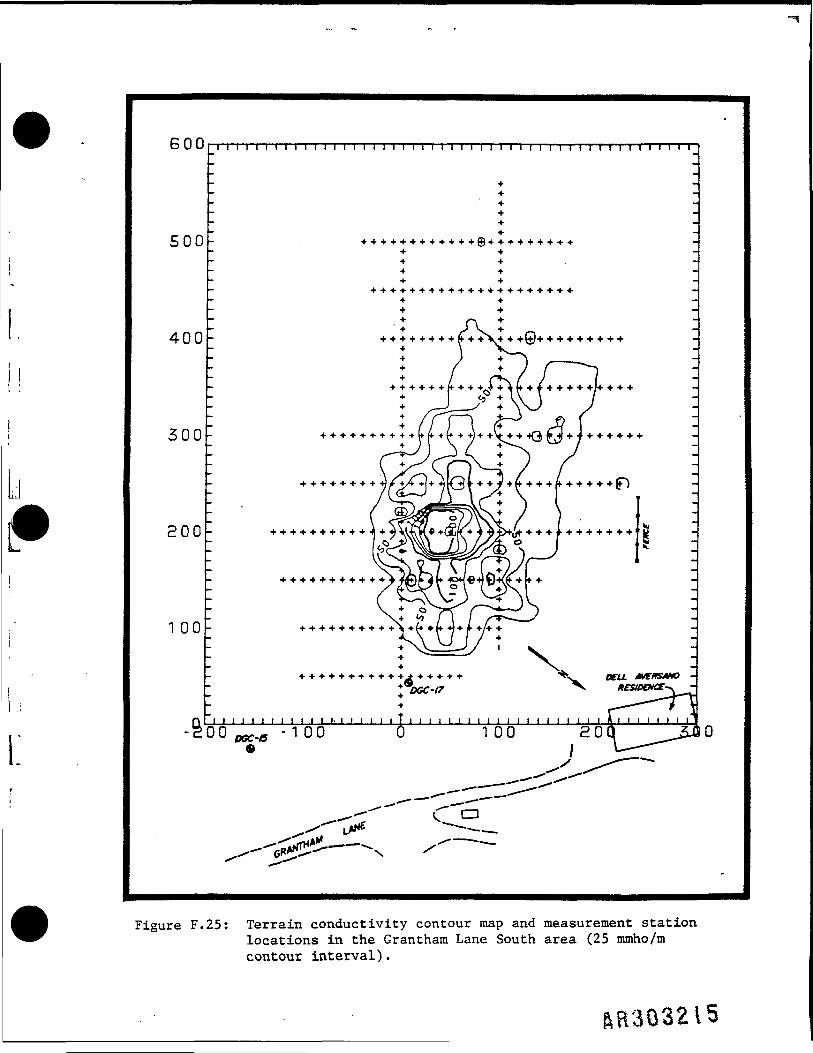
*J LJ w ~~~i t ""t" "" "t"""t T 1 I 171 I I 1 f t "'l 1 T 1 I 1 T I . i I 7 ~"T I I I 1 T I T J T TT T T 7 1 i 1 V T
500 -
400-
300-
200-
1 00-
•f-r-f-f-f-r-r-f
f-r-f-f-f-ff)
+®«— ~
i t i i i i i i i i i> i i i i i i i i i i i i i i i i i i i i i t i i i i * i i i i t i i00 IWC-45 'TOO
Figure F.25: Terrain conductivity contour map and measurement stationlocations in the Grantham Lane South area (25 mmho/mcontour interval).
IB303215

O w U i r t i i T r i i r i i i i i i Y I \~~~t~ i i i i i i i i i T t ij i i i i t i i T~i"~ I i i i i i i T
500-
400-
300-
200-
1 00-
Figure F.26: Magnetic intensity contour map and measurement stationlocations in the Grantham Lane South area (500 gammacontour interval).
IR3032I6
Interpretation was done by comparing anomalous areas defined bythe EM-31 and magnetometer surveys. The relative magnitude andshape of the anomalies were used to make inferences concerningthe cause of the anomalies. Field observations made during thegeophysical survey were also helpful in interpreting the data.
Nature of the Upper Potomac Confining Clav
During the first phase of work, soil borings confirmed theabsence of the confining clay between sands of the Columbia andUpper Potomac Formations near the drum disposal area. Verticalresistivity soundings and terrain conductivity traverses usingmore deeply penetrating EM-3 4 instrumentation were performedduring the second phase of work in an attempt to evaluate thepresence or absence of the confining clay layer.
Two resistivity soundings were made to determine the verticalvariation in resistivity of the subsurface materials. Thesoundings were performed at the locations of wells DGC-2 andDGC-3 to provide geologic control data. Both sounding lineswere located to minimize topographic and vegetative variations.
The results were plotted as sounding curves of apparentresistivity in ohm-meters versus electrode spacing (Figures F.27and F.28). The curves were interpreted using the semi-empiricalBarnes Layer Method. Results are shown in Figures F.29 and F.30and are discussed in the following section.
Four terrain conductivity traverses in the drum disposal areawere performed using EM-34 instrumentation. The traverses werelocated between existing borings to provide geologic control andaid in the interpretation. EM-34 traverse #1 was locatedbetween DGC-2 and DGC-3, traverse #2 between DGC-3 and B-l,traverse #3 between B-l and DGC-2 and traverse #4 between DGC-2and DGC-4. The horizontal dipole data were more stable and lessnoisy than the vertical dipole data.
ftR3032!7
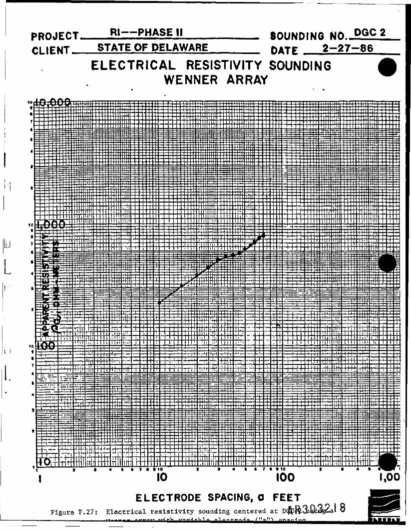
Rl—-PHASE II ftAiikirMijft im DGC 2r
C
10i•T
*
1
4
I I
'I
Kl
—1 4
I
I
M "•
. 7
(
t
' 4
1
• ICWT STATE OF DELAWARE r TF 2-27-86ELECTRICAL RESISTIVITY SOUNDING (ft
WENNER ARRAY
E E E E E E E r i EEEi I : E E E E:E!||=E=EEE ^ E E E E E E E E E i EE| ?E E = f
54,." '~~ ' iLi :—: - . -rr — U-i -- i -• -r -*• i ' i ' -•--M' -^ "T
ij~ ' -r ' ' . ; , i ' i . i 1 j 1 1 , i i i i | :
jj g|S[iii|3iiiil|ii|i|||ii
|[1 gzp m Ei lEE Ej;:: Egg,:::
T* ' "it" Hi 13 " 1 [<«'•'•'" 1 ! -----4--- jj , j yr--1---"Tr1- i ,11 MTT nji T i 'in r" _-_ T • • • '• ,!£0-:—— "r~ ~T -H: ~ 4= ~ ~ ~ -4- :— — ~ =±
-j ——— -_r- -r-—— T fr|T fl. •{ j jl jij 1, ; j __ j __ j , J | . I, 1 -H, 4
-p--r— rjr r g= ui:.--: - - - - — -• -• - : - — _-._.-..... ..S ._
at IT • ! i T i i _^_ iT"Hi iffi r... i ..... j.; .u .. ^ ^
:: zirai::::::::---:::::::±±:i;;:::::: ::::::::::::-;
::::::: ift ::::::::! = :::::::::::::;::::::: :::: ::::::::::::g!::::::::i:-r :::::: :SS ::::: i:::ij :::*::....... _j|. -. .-....____........... ... ......... j rj, ___...
E:ffli||::i :::::::S::|::::::S5F-r|-f-.. h ~ .. 1 ..i " _ ^ ...j.,., ..,, ..„ i! h id ~> ..
- • -j-h-*- -^ -J- -r 4- 4- — }— j — - — - - . 14. f-U — U-L --•• -^4 -+- -^ -P
[T i ,, ' • Tit . ; il ii'1 T I ' . i it .1 ' • i . ' "Ti | , i !] -Hi | 1lie ' ' i 1 1 j : i 1 ' 1 ' • - ' ' ' j
! • • i t , i ! i 1 1 1 1 |l| | i i • 1 1 . 1 i I
4-L | 1 ' —— 1 - - . - -p .. — , — p.— :- J_ -j- j i j \ Lr« ! | | | y.-- Lri —U ---(-,
l-"tt^--"T- - — -J-t Ttii-iii jj i . I "!:M1;! • i 1 1, : •!, 1! • ! ' *
~ f » 4 t * T i » 1 0 t » 4 » * 7 « t t O t » 4 » «* rPi <
I 10 100 1,00ELECTRODE SPACING, 0 FEET S3
Figure F.27: Electrical resistivity sounding centered at D< f* '$vek&g(-a' " pP ^

* & *. * ' LRI-PHASE II__________ SOUNDING KQ DGC 3r
!
1C 11 J
I 't
1,0
*'l~-x
H ':L :
6
. . 4
X
LIPHT STATE OF DELAWARE HATLT 2-27-86ELECTRICAL RESISTIVITY SOUNDING
WENNER ARRAY
= = "::::: :::: ±P P-: %t te -:$::::= = = = :::::: ::iit4:::
T; 1 1 ... ..... Lli x. ----..-.—-------••..... <y. .--
"ijn"?-""': -t.: ic:::::4::::ii:ii:iii;i--iiii"i:ii: ::::":
IK En lJ£:-:--£^± iT~En--- i;:-|Sj-^^^susti^^-^is^lggJlitt
-i —— i-r- -r-H-5- i-rrt t- -"j MT .,,;-••••••••- , •-- r-T '!" '! ! i
iv" "1:- g:B±:itiT-;4-T-J::--==""± ^-4— •~j~ ~7* "T"1 '- •• i** 7 *• ,"j j!" "*1 ~'t i, ill , i , t , i
Tw"T~nllij jj it TTi' lit; ' j TIT
;:::::: ifo:::::r.:: ~:|:::::::::: j: :::::::::; :::::$::-• t**- TJ-T -- -- j T™ p-H- -H---— -•r^'ri----...... ••• ^TT;--
:!! ., , , , - ,.., ,-.,,..... r , ... L..,>-- rL4 r r- - - - - - - -r -'-f-p-f- -r^--- 4j* .-T ' l i t - - + • ilrj -4- -i- -r-
4 4-H tY -- -r -r -1- -H-H- -*4r+ -H+- --^-------ffiTfj-t-r---
1 _LI • I ; , ! :j i j ! ! : ! ' ! ! -,- T1 I^j -^ ^ , 1 : t M li i, ! ! 1 1 1 1 T i
r 1 1 1 1 • , T r i - j » » ' i * 1 1 1 i ; i i t •• • .
4- -^— — —— - ——— — . -i- -r —— —— ' ' ' —— •—r-<* -~- — - —— 1 - ———— L i | |'| -r-r--- —— ——
1 --L-. 4 ~ ~ ~~ ~~. Z - p _ - -.—f-r r-rri -j-p - •-•• '-IT -^- -- -
4--T 7H", T- ' ~ -T i" ttr rf -J-JTT rjt ~"- , T i! ,,i '• ii,i.i :li TI _T ,...jT±
1 10 100 I.OCELECTRODE SPACING, 0 F|EJ032lg Bg
Figure F.28: Electrical resistivity sounding centered at DGC-3 using a Wenner (H ^

IMIII!•IOkCll»M C
b A R N E S L A Y L6550. + "
IIII
5650. «•' I
II1
4751. «•IIII
3852. +I1I1
2952. »III
v. It 2053. +
1 \S 1154. +
0. t10.0 15.0 20.0 25.0 30.0 35.0 4O.O 45.0 50.0 55.0 60.0 65.0 70.0
DEPTH (FEET)
Figure F.29: Barnes layer model of resistivity versusdepth at DGC-2 .

IMIIIIIClOfcCllftM COK'
Resi»tivity B A R N E S L A Y E R270. *
**.40
Ce
4Q
*•>.
t>
£Sic
* **••i •••ii
239. +III1
209. 41 ***j ***
I ***
179. + •»*
I *••i4a. + •••
i *•«
n. ^ ————— « ———— 1 ———— l ———— 1 ———— 1 ———— t ———— 1 ———— 1 ——
»••*••••****• •*•• •••• * «•
»*** »*•» **••
10.O 15.0 20.0 25.0 30.0 35.0 40.0 45.0 50.0 55.0 60.0 65.0 70.0 80.0 100.0
DEPTH (FEET)
Figure F.30: Barnes layer model of resistivity versusdepth at DGC-3.
RB3Q3221
The 20-meter intercoil spacing was used for each EM-3 4traverse. The intercoil spacing used was selected to provideterrain conductivity information incorporating the effects ofthe Upper Potomac confining clay. Readings were obtained at25-foot intervals along the traverses using both the horizontaland vertical dipole orientations. Thus, a maximum effectivedepth of investigation of 50 to 100 feet was achieved. Thegeologic contact between the Columbia and Upper Potomacformations in the drum disposal area ranges from 30 to 40 feetbelow land surface.
Results of the terrain conductivity surveys were plotted asprofiles of terrain conductivity in mmhos/m versus distance(Figures F.31 to F.34). Results are discussed in the followingsection on interpretations.
8R3G-3222

Terrain Conductivity Profile it fEM-34
i
i:i ! i.
iM § 20 -1
o
Li 2^ ^ E
[W ~ »-
1ii 10-
: 1
i5 -
1.
0 -
• ———— • Horizontal
x ———— x Vtrtfcol
/>/ \
• "7 »x~xx l- - / *-"X
j.-/.*—*-*/' Vju--.x~ "/-OGC-2 .X */ * S 1
\ x\ /
V7
1 1 1 1 10 KX} 200 300 400 500
DMone* (tot)
_ NORTHWEST SOUTHEAST^^^ Figure F.31: Terrain conductivity profile (EM-34 No. 1)^^^ in the vicinity of the drum disposal area.
RR303223

Terrain Conductivity Profile it 2EM-34
30 -
x———x vertical• i >25 -
* "
20 -
15 -
10 -
i.5 -*™ 1 11 11 11 1IIIIlij
1 1 —— „ ——————— , ——————— ,0 K» 2OO 300 4OO 50O
Diatom* (f ««t)
SOUTHEAST NORTHWEST
Figure F.32: Terrain conductivity profile (EM-34 No. 2) inthe vicinity of the drum disposal area.
&R303221*

Terrain Conductivity Profile #3EM-34
Ill oe
30 i—x——»——x\\V\ •————• Horizontal^ *————x Vtrtical
25H \*\\
\
\\\\\
is -
oe 10'5
5-DGC-2
I I I T I100 200 300 400 500
Di»tonc«
EAST WEST
Figure F.33: Terrain conductivity profile (EM-34 No. 3) inthe vicinity of the drum disposal area.

s 15
10
Terrain Conductivity Profile #4EM-34
30 -
•————• Horizontal fx————x Mirtical '
25 H '
/
/
-, 20
1 ' il' /
/
• /'/\ /x
//\ S' \ /
/ \\./.vDGC-2-. / '* _/ -OGC-4
/M/'•'l sM/ /
I I I ——————I——————————|0 100 200 3OO 40O 5OO
Oistanct (f«»t)
SOUTHWEST NORTHEAST
Figure F.34: Terrain conductivity profile (EM-34 No. 4) inthe vicinity of the drum disposal area.
HR30322S

F.4 Survey Findings and Interpretation
Plate 3 displays the major interpretations of the geophysicalresults including the anticipated locations of concentrations ofburied steel drums, landfill boundaries at tested locations,seismic refraction depths, and other anomalies of potentialhydrogeologic significance. A brief explanation of theinterpretations is provided below including the specificobjectives described in Section F.3 and the presence of possibleclay layers and leachate plumes.
Location of Buried Drums in the Drum Disposal Area
Delineation of buried steel drums in the northern landfill areais based on a combination of terrain conductivity andmagnetometer contour maps and site observational data. The twogeophysical techniques complemented each other well in depictingthe large and complex (approximately 160 feet by 340 feet)anomaly inferred to be the location of buried drums. Thisanomaly is defined within the 58,000 gamma magnetic contour line(Figure F.5), the 25 millimho per meter EM-31 contour line(Figure F.2), and the 5.0 millimho per meter EM-31 differencecontour line (Figure F.3). Although the anomaly is attributedpredominantly to steel drums, much of its complexity may also becaused by other sources such as scrap metal, drum fragments,etc. Because of the known occurrence of steel drums in thisarea, however, the source will be referred to as drums unlessotherwise indicated.
The lateral extent of the drums appears to be within the regiondefined by the construction access road and fence which wereinstalled as part of the 1984 surface drum removal operations.Anomaly patterns suggest where the major drum concentrations arelikely to be situated within the drum disposal area. Patternsare indicative of subsurface variations caused by changes in the
RR3Q322?
type, depth, thickness or distribution of buried metal or otherconductors. Unfortunately, magnetic/electromagnetic inter-ference from the fence and adjacent railroad tracks may beobscuring the magnetometer data for a distance up to 60 feetfrom the fence and the conductivity data for a distance up to 25feet thereby preventing reliable interpretations in this area.
The presence of concentrated buried metal is suggested by thesmall closed contour lines representing magnetic highs andconductivity highs and lows, by the density of contour lines,and by lobate anomaly patterns. As a first approximation,concentrations of drums can be expected within 10 feet laterallyof the magnetic peaks, points of maximum magnetic field gradientand conductivity lows. The type of pattern displayed in thesouthern part of the large anomaly is typical of shallow sources(probably within approximately 10 feet of the ground surface)and the broader lobes are probably indicative of deepersources. It is noteworthy that numerous small drum fragmentswere observed during the field survey in the southern part ofthe survey, supporting a shallow source interpretation. Thisinterpretation does not preclude the possible presence ofshallow drums in the north and deep drums in the south.
Due to the complexity of the anomaly and its sources, it is notpossible to determine the depth and mass of the concentrationsof buried metal. However, rough rule of thumb estimates suggestthat sources may be distributed from less than 5 feet to 40 feetdeep, in agreement with anticipated depths. The maximummagnetic anomaly observed was on the order of 8000 gammas abovethe background magnetic field intensity of approximately 55,500gammas. This very large anomaly approaches the approximate10,000 gamma anomaly limit upon which many simplifyingassumptions for proton precession magnetometer search theory arebased. However, to give an approximate idea of the mass of
1R3Q3228

buried iron or steel required to produce such anomalies, asingle 35-pound steel drum may generate an anomaly on the orderof 30 gammas at a depth of 2 feet, 5 gammas at 10 feet, and 1.5gammas at 20 feet. It is not recommended that these values beextrapolated to an 8000 gamma anomaly because the actualquantity of drums may be substantially greater or less.
The combined terrain conductivity and magnetic contour mapsindicate several subtle features that are pertinent to siteconditions. They are described as follows:
1. An approximate 190-foot long by 25-foot wide strip of zeroconductivity and relatively non-anomalous magnetic intensitycrosses the north and east portions of the large anomaly andis centered at stations 2010N/375E and 1950N/480E. The zeroconductivity is probably indicative of shallow (less than 5to 10 feet deep) metal. Scattered surface metal observed inthis area supports this explanation. The apparent absenceof a corresponding magnetic anomaly may suggest the presenceof non-ferrous metal or very small masses of near-surfacemetal. It may also be indicative of masking by the adjacentlarge anomaly.
2. Two easterly trending troughs in the magnetometer data inthe large anomaly suggest discontinuities in the drumdepositional pattern or areas where drum concentrations maybe minor. High conductivities in these areas suggest thatsome non-ferrous metal or conductive leachate may bepresent.
3. A curvilinear pattern of relatively low magnitudeconductivity and magnetic anomalies is evident west of theburied drums and is shown on Plate 3. This pattern isparticularly evident in the conductivity difference plot,Figure F.3, and supported in a high resolution magnetic
ft8303229

intensity plot of the western side of the drum disposalarea, Figure F.6. The pattern is manifested as acurvilinear clustering of small isolated anomalies possiblyattributed to scattered near-surf ace metal. The anomalouszone is roughly parallel to the apparent large drum anomalyand may be related to the site waste disposal/drum removaloperations. The anomalous zone also reportedly bounds asaltation pond related to sand removal and sand washingoperations.
Landfill Boundaries in the Inert Disposal Area
Plate 3 shows the location of magnetic and conductivitytraverses and disposal area boundaries interpreted from thosetraverses. The traverses indicated that landfill boundaries aregenerally associated with physical features such as vegetationor topography, with a few exceptions. A description of eachtraverse is provided below.
Terrain conductivity profile |1 (Figure F.7) was the preliminarytraverse made at the site. Its purpose was to identify the areaof buried drums and the nature of the adjacent low-lying area aswall as test the usefulness of the method. The presence of theburied drums is readily apparent due to the high magnitude andvariability of the measurements over the disposal area. Thedata in the low-lying grassy area suggests a difference insubsurface properties from that observed in the apparentlyundisturbed wooded area to the west, which is probably underlainby dry sand. The difference may be attributable to a contrastin soil properties; the low-lying area may be clayier, siltier,and wetter than the wooded area.
Terrain conductivity profile #2 (Figure F.8) was conducted todetermine the nature of the eastern boundary of the inertdisposal area. The data suggest that the landfill boundarycorresponds with the topographic expression, as expected.
A8303.230
Terrain conductivity profile #3 (Figure F.9J and magnetometertraverse #1 (Figure F.19) were conducted to verify thetopographic relationship suggested by TC profile #2. These twotraverses were run a short distance north of TC profile #2across a plateau apparently situated at the top of the"landfill". Surprisingly, the data suggest that the plateau isunderlain by relatively clean soil and the inert disposal areaboundary is situated approximately 100 feet west of where it wasoriginally anticipated. The actual boundary appears to beassociated with a relatively small (approximately 2 to 4 feet)topographic rise. The plateau probably is underlain by sandfill or spoil from the former sand mining operations.
Terrain conductivity profile #4 (Figure F.10) and magnetometertraverse #2 (Figure F.20) were conducted to investigate thenorth boundary of the inert disposal area in the vicinity of theopen sand pit. The data indicate that the boundary in this areais associated with the major topographic slope, as anticipated.
Terrain conductivity profile #5 (Figure F.ll) was performedalong grid line 12 at the southern edge of the inert disposalarea where topographic expression was subdued. The data suggestthat the edge of the landfill may be in the vicinity of station10+60, associated with a small topographic break, but theabundance of surface metal in the area impairs the reliabilityof this estimate.
Terrain conductivity profile #6 (Figure F.12) was conductedoutside the inert disposal area and in the open sand pit. Thepurpose was to provide additional background information toevaluate the natural variability of the sandy soil in contrastto the inert area. The data indicate low, nonvarying terrainconductivity as anticipated.
HH30323I
Terrain conductivity profile #7 (Figure F.13) and magnetometertraverse #3 (Figure F.21) were conducted for a similar reason asprofile |6 above, except these profiles were made tocharacterize the anomaly pattern within the inert areaboundary. These transects were run along a seismic refractionline to assist with the interpretation of the seismic data. Asexpected, the terrain conductivity and magnetometer data in theinert area had relatively high magnitude and/or variabilityindicating heterogeneous, predominantly non-metallic fill. Theanomaly pattern suggests a change in the nature of the fill inthe eastern 50 feet of the traverses.
Terrain conductivity profiles #11 (Figure F.17) and #12 (FigureF.18) and magnetometer traverses #5 (Figure F.23) and #6 (FigureF.24) were conducted during the second phase of the RemedialInvestigation to provide additional information on the westernboundary of the inert disposal area. The data indicate that thelandfill boundary in this area is associated with the majortopographic slope as shown on Plate 3. The topography of thewestern boundary is indicative of man-made borrow pits withridges as illustrated on the base map. The extra traversesperformed during the second phase of work were designed toassess these areas of potential landfilling.
landfill Thickness in the Drum and Inert Disposal Areas
Interpretation of the seismic refraction spreads in the drumdisposal area utilized nearby boring B-l for subsurfacecontrol. The presence of two layers is indicated. The upperlayer, interpreted as loose silt and sand with a seismicvelocity of approximately 1200 feet per second, overlies adeeper layer of medium dense, possibly saturated sand with avelocity of approximately 4500 feet per second. The interpretedthickness of th© upper layer ranges from 22 feet to 30 feet.The data in the drum disposal area suggest that the interface
ftH303232
between the two layers slopes towards the center of the site atthe edges of the study area and is relatively level in thecentral portion.
Seismic refraction data indicate the fill in the inert landfillis very heterogeneous and transmits seismic waves poorly. Inmost cases, the signal from the wave traveling through air wasmore apparent than the wave transmitted through soil. As aresult, the interpretations for this area are judged lessreliable than those in the drum disposal area.
The seismic data identified the presence of one to two layersalong the spread conducted in the inert landfill; two layerswere apparent at the southwest end of the spread, but only onewas resolved at the northeast end. For the two layer case, theupper layer had a velocity of 1150 feet per second and isinterpreted to be loose fill. The underlying layer has avelocity of approximately 2700 feet per second and isinterpreted to consist of unsaturated sand or clay, possiblyfill, at a depth of 26 to 33 feet.
Location of Buried Metal and Landfill Boundaries in the GranthamSouth Area
The delineation of the lateral extent of landfilling and areasof concentrations of buried metal in the Grantham Lane Southarea were based on the EM-31 and magnetic.contour plots and siteobservational data. The lateral extent of landfilling isrelatively obvious from field data. The wastes in the GranthamSouth area are relatively exposed (i.e., uncovered), especiallyon side slopes. Steep-sided, "clean" slopes of the sand pitedges flank two sides of the wastes. The waste materials wereapparently dumped into the sand pit from the upper lip adjacentto Grantham Lane. The top of the waste material is flush (withrespect to elevation) to the surrounding land to the northeast.
HS303233

The terrain conductivity data (Figure F.25) show a large,relatively smooth anomaly created by the wastes. The 25 mmho/mcontour line delineates the approximate lateral limits of thelandfilling. Areas beyond and outside the 25 mmho/m contourappear relatively clean based on field observations.
TC values in excess of 200 mmhos/m are recorded in the centralportion of the waste (i.e., the southern part of the flat upperbench). A broad low anomaly (i.e., generally 50 mmhos/m) isobserved in the western portion of the waste and is attributedto scattered debris observed on the floor of the sand quarry.Zero terrain conductivity values associated with the high valuesare notably absent unlike the survey performed in the drumdisposal area. This is attributed to the presence of moredeeply buried (i.e., 10 to 15 feet) metal objects and possiblyconductive leachate.
The magnetic intensity contour map (Figure F.26) is complex.Background values in undisturbed areas range from 55,300 to55,450 gammas. The highest value obtained exceeds 58,500 gammasand is located in the north-central part of the waste area.This 3000 gamma anomaly is very localized (i.e., only one datapoint) and is not reflected in the terrain conductivity data.Thus, this metallic anomaly is attributed to a discrete, large,shallow source.
A large, broad, magnetic anomaly is present in the southeasternpart of upper bench of the waste. Numerous readings in excessof 58,000 gammas were obtained. This magnetic anomaly may beattributed to a large, deeply buried metallic source or ashallower, more extensive source (i.e., layer). When comparedto the TC data, the center of the magnetic anomaly is 50 to 60feet south of the large EM-31 anomaly. The two anomalies arelikely not due to the same source or source type.
«fl30323-i

Nature of the Uppermost Potomac Confining Clay
The vertical resistivity soundings and EM-34 profiles in thedrum disposal area were performed to assess the feasibility ofeach method in evaluating the presence or absence of the UpperPotomac confining clay. The methods were applied in the areaswhere geologic control was available in order to assess theeffectiveness of each method.
The results from the two resistivity soundings performed nearDGC-2 (Figure F.27) where the confining clay is absent, andDGC-3 (Figure F.28) where the confining clay is present areinconclusive. An electrode spacing appropriate to investigateof the confining clay layer could not be determined; thus, aresistivity survey was not performed.
The four EM-34 traverses performed between existing borings(B-l, DGC-2, DGC-3 and DGC-4) in the drum disposal area showedencouraging results. No confining clay is reportedly present atboring DGC-2. Confining clay is reported at the other threeborings (B-l, DGC-3 and DGC-4). EM-34 traverses 1, 3, and 4(Figures F.31, F.33 and F.34, respectively) indicate increasingterrain conductivity away from boring DGC-2. The increasing TCvalues may be due to the presence and/or increasing thickness ofthe Upper Potomac confining clay. Thus, TC values of 5 to 6mmhos/m may be indicative of no confining clay and higher valuesmay be associated with confining clay of variable thickness. Ifso, then the plots of the traverses indicate that the "zeroarea" may end approximately 50 feet away from DGC-2 to thesoutheast and 100 or more feet away to the northeast. However,these interpretations should be considered uncertain.
ft8303235

Possible Clay Layers and Leachate Plumes
The project objectives did not initially include search for claylayers and leachate, but locations for these possibleexploration targets emerged from the data collected. They aredescribed below according to the traverses on which they wereidentified.
Terrain conductivity profile #8 (Figure F.14) and magnetometertraverse #4 (Figure F.22) were conducted along the dirt roadalong the east side of the site to characterize the subsurfaceconditions along the landfill's eastern boundary. Theinformation was used to help interpret landfill boundaries. TheEM-31 profile indicated a zone of elevated conductivity betweentraverse stations 400 to 690. It is possible this zone extendsto station 200, but this portion of the data is masked byinterference from a power line. The cause for the anomaly isuncertain, but may be attributed to a clayier soil texture or anincrease in soil electrolytes or moisture content. The edge ofthe anomaly at station 690 is very abrupt and may represent theedge of a near-surf ace clay layer, a change in road material ora leachate plume. Considering that boring B-4, located withinthis anomaly, indicates a clayey subsurface, it is likely thatthe anomaly is related to the lateral extent of a clay layer.
Terrain conductivity profiles #9 (Figure F.15) and #10 (FigureF.16) were made in the area between the inert landfill and drumdisposal area. Profile #10 was a partial repeat of #9 forquality control to determine if the conductivity differencetechnique would provide different results, which it did not.Profile #9 indicates a zone of elevated conductivity fromtraverse stations 300 to 400. The zone is associated with aleachate area observed on the ground surface and, therefore, theconductivity data indicate the possible lateral extent of thisplume.
483-03236
Appendix G
Monitoring Well Data
58303237
Lu Soil Classification Explanatory Sheets
AR303238
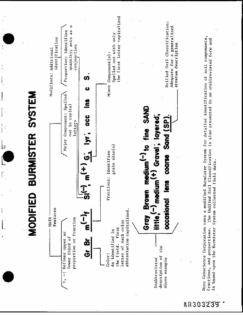
UJ
(OccUJ
,L
cn tncu ro PI TJ cc'H r-l C. CJc ro
jj o uU iJ CU Cc r o c x: >j t n c Scu o jj cu w cu IH
TJ •« -H -H JJ CO 6C• 3 JJ
CJ /—•. CU CJ CflCn JJ rH
C JJ 3 ^ 3OC-r-1 J J Q 4 J - H O C Oro c c cn • o uj cu
3 O CU T) >J COO- U C CU -H <l) -
O O r-l u-i T3 JJ SO- • 0.rH CU CO 3Q ^^k c CU CU *H 3 JJ
O C. X! u_i crcu * cj co jj -i-i cuC T3 _
V4 3 < 03Oe
JJ Cc rocuC EO rJf") Oe ujou -acu
O XI
c roo c•H 3jjro cu ro
C T301 (U-a jj•H C
Q)T3 tnCD 0)
•rt C.toJJ o0) W•O r-lroS-4
o wU- >H
e c,01 OJJ -Hcn jj>i ro •c/2 u ro
•H JJrJ UJ (0
•" ro
•a o cu^ ^ "~~ ^ " ••» ~ ^ CJ C.O W
O L_co 2 8 5 ~ - •««U J v * f c 8 6 ^ ^ " ^••• •• ^ o uj o|§ tn —— | O S c °U L ? 1 •*- -2 J-«S rosg—~ — -1 *'•" " 9k A% *"• cn cu jjz w ^x c I IH C* ™ «' cu x: cnHJ to (^ o I ——I urn O - E C W H > ,O< c u - H «M-> o r o \ W £ j i / 3 w
SCI< a P jj^.H\r«j(CS/ c < uo cn cu.. _ ro \___________J -H c jjo uj •<-( x! o jj o tn
U-i -O to. CJ to -H -HSJ O I- JW CU CO C }jJJE(D O MM -H CU O O rn rJc. -a IU u- • -H c. o 3& |j c __ •HTaujjj cu i- a. ca3 -H o —~~ jj i— o ro — o ox: -H •• c cu -H jj cj >j cucn jj jj ff% •• cu -H ij > c. x:C ) J O O ' H J J ) j T 3 O O ) CJT3•HCUC. r H C U J J X l C U r H ' , C C Cuj?o _ o c n x : c u x s J J G O . c u r o ccu c ^ ^^ cj<;jJr-iro r o o E - H O .~ • - ro u • 3x cn cn
CU C. CU O C T3(J -H CU O CUX! ij cu cj -H cnXi u > jj ro+ ro w c c o xicox; c ro3 -o ro 3 ^ w
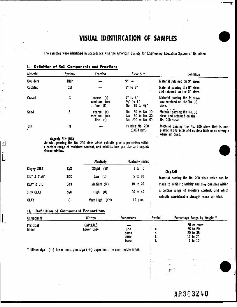
VISUAL IDENTIFICATION OF SAMPLES
The samples were identified in accordance with the American Society for Engineering Education System of Definition.
I. Definition of Soil Component* and FractionsMaterial________Symbol______Fraction__________Sieve Size ____________Definition. . — . . j .,————————.———— •——.Boulders Bldr — 9" + Material retained on 9' sieve.Cobbles Cbl — 3" to 9" Material passing the 9* sieve
and retained on the 3* sieve.Gravel G coarse (c) 1" to 3' Material passing the 3* sieve
medium (m) %" to 1" and retained on the No. 10fine (f) No. 10 to %" sieve.
Sand S coarse (c) No. 30 to No. 10 Material passing the No. 10medium (m) No. 60 to No. 30 sieve and retained oo the
fine (f) No. 200 to No. t$0 No. 200 sieve.Silt $ — Passing No. 200 Material passing the No. 200 sieve that is non-
(0.074 mm) plastic in character and exhibits little or no strengthwhen air dried.
Organic Silt (0$)Material passing the No. 200 sieve which exhibits plastic properties withina certain range of moisture content, and exhibits fine granular and organiccharacteristics.
Plasticity Plasticity IndexClayey SILT Cy$ Slight (SI) 1 to 5
Clay-SoilSILT & CLAY 5&C Low (L) 5 to 10 Materja| _mlng ^ m .]m whjch can b(,
CLAY & SILT C&$ Medium (M) 10 to 20 made to exhibit plasticity and clay qualities within
Silty CLAY $yC High (H) 20 to 40 a certain ranee of mofsture content' and whichexhibits considerable strength when air-dried.
CLAY C Very High (VH) 40 plusI
II. Definition of Component ProportionsComponent_________________Written_______Proportions____. Symbol____Percentage Range by Weight *Principal CAPITALS — 50 or moreMinor Lower Case and a. 35 to 50
some s. 20 to 35little I. 10 to 20trace L 1 to 10
* Minus sign (—) lower limit, plus sign (+) upper limit, no sign middle range.

III. Glo»»ory of Modifying Abbr»vioHon«
Category________Symbol______Term______Symbol______Term______Symbol______Term___A. Borings U/D Undisturbed B Exploratory A Auger
B. Samples C Casing L Lost U UndisturbedD Oenison S Spoon W WashO.L Open End
C. Colors bk black gn green wh whitebl blue or orange yw yellowbr brown rd red dk darkgr gray tn tan It light
D. Organic dec decayed o organic veg vegetationSoils dec'g decaying rts roots pt peat
lig lignite ts topsoil
L Rocks LS Limestone rk rock Shst SchistGns Gneiss SS Sandstone Sh Shale
F. Fill and bldr(s) boulder (s) cbl(s) cobble(s) gls glassMiscellaneous brk(s) brick (s) wd wood misc miscellaneous
Materials cndr(s) cinder (s) dbr debris rbl rubble
G. Miscellaneous do ditto pp pocket ref refusalTerms el, El elevation penetrometer sm small
fgmt (s) fragment(s) P. I. Plasticity W. L water levelfrqt frequent Index W. H. weight of hammerIrg large P pushed W. R. weight of rodsmtld mottled pressedno rec no recovery pc(s) piece (s)pen penetration rec or R recovered
H. Stratified alt alternatingSoils thk thick
thn thinw withprt parting — 0 to 1/16" thicknessseam seam — 1/16 to %" thicknesslyr layer — ^ to 12" thicknessstra stratum — greater than 12" thicknesswd c varved Clay — alternating seams or layers of sand, silt and claypkt pocket — small, erratic deposit usually less than 1 footIns lens — lenticular depositocc occasional — one or less per foot of thicknessfreq frequent — more than one per foot of thickness
flR3Q32UI

UNIFIED SOIL CLASSIFICATION SYSTEM. (ASTM D-2487)
Major Divisions
Coane-giraiined so»i
(More than
half of material h
turger ttmn No. 200 sieve size)
Bite-grained so
Mt(More than
half material is smaller thin No. 200 sieve)
Gravels
(More than
half of
coarse fraction is
larger th
an No. 4 si
eve siz
e)
Sands
(More than
half of coarse fraction is
smaller-than No. 4 si
eve size)
Clean gravels
(Little or no fines)
Graveltwilh fines
(Appreciable amount
of fines]
Clean sands
(Little or no fines)
Sands with
fines
(Appreciable •mount
ol fines)
Silts
and clays
( Liquid
limit lew
than 50)
Silts a
nd clays
(Liquid
limit greater rhan 50
)
ill
GroupSymbols
GW
GP
dGM* —
u
GC
SW
SP
dSM* —
u
SC
ML
CL
OL
MH
CH
OH
Pt
Typical Names
Well-graded gravels, gravel-sand mix.tures, little or no fines
Poorly graded gravels, gravel-sand mix-tures, little or no fines
Silty gravels, gravel-sand-silt mixtures
Clayey gravels, gravel-sand-clay mix-tures
Well-graded sands, gravelly sands, littleor no fines
Poorly graded sands, gravelly sands,little or no fines
Silty sands, sand-silt mixtures
Clayey sands, sand-clay mixtures
Inorganic silts and very fine sands,rock flour, silty or clayey fine sands,or clayey silts with slight plasticity
Inorganic clays of low to mediumplasticity, gravelly clays, sandy clays,silty clays, lean clays
Organic silts and organic silty clays oflow plasticity
Inorganic silts, micaceous or diatoma*ceous fine sandy or silty soils, elasticsilts
Inorganic clays of high plasticity, fatclays
Organic clays of medium to highplasticity, organic silts
Peat and other highly organic soils
Laboratory Classification Crittria
lercentages of sand and gravel from
grain-size curve.
in percentage of
fines (fraction smaller than No. 200 sieve s
ize), coarse-grained
sified as follows:
5 per cent
GW, GP, SW, SP
12 per
cent
GM, GC, SM. SC
r cent
Bordarline ca
ses requiring dual symbols'5
if!Js£Q Q S
D60Cu " —— greater than 4; Cg • (Oao)
Not meeting all gradation requirements for GW
Atterberg limits below "A"line or P.I. less than 4
Atterberg limits below "A"line with P.t. greater than 7
Above "A" line with P.I.between 4 and 7 are border-lint cases requiring use ofdual symbols
060 (Oso 1C_ * —— greater than 6; C,. • —————— between 1 and 3°10 0|0 X 0«o
Not meeting all gradation requirements for SW
Atterberg limits above "A"line or P.I. less than 4
Atterberg limits above "A"line with P.I. greater than 7
60 1 —— - —— | —— i
so — — —
x 40 —— —— ——I£ 30 —— —— ——U
rt£ 20 -
10-CL
— -CL-ML-fflffilrffiffiP
0, 10 20 3
Limits plotting in hatcli lzone with P.I. between 4and 7 are borderline casesrequiring use of dual sym-bols
Plasticity Chart
/
ML(
Xr/and3L
/
CH ./
£OH and MH
0 40 SO. 60 70 80 90 100Liquid limit
M"Division of GM »nd SM groups into subdivision! of d and u »r« for roads and »irfiilds only. Subdivision is bated on Attcrbcrf limits; <uffix d u»»d 'L.L. Is 28 or less and the P.I. is 6 or !•», the suffix u used when L.t. is greater than 28.Borderline classifications, used for soils possessing characteristics of two groups, are designated by combinations of group symbols. For example:GW-OC, wall-grided gravel-sand mixture with clay bindir.