Download - Timing and stability in cellular automata - tbi.univie.ac.at · Timing and stability in cellular automata Konstantin Klemm Bioinformatics Group University of Leipzig, Germany Konstantin

Timing and stability in cellular automata

Konstantin Klemm

Bioinformatics GroupUniversity of Leipzig, Germany

Konstantin Klemm (Leipzig) Timing & Stability in CA 1 / 25

Definition

finite set of states S , often |S | = 2

mapping (“rule table”) f : Sz → S

a lattice of n sites with coordination number z where site i hasneighbours a(i , 1), a(i , 2), . . . a(i , z)

time-discrete dynamics of lattice site i

si (t + 1) = f [sa(i ,1)(t), . . . sa(i ,z)(t)]

All lattice sites are updated in synchrony.


Purpose

Computer Science: Models of computation,e.g. “Game of Life” and “rule 110” are Turing-complete.

Artificial Life: Study of self-reproducing structures

Physics: Abstractions of spatio-temporal dynamics, pattern formation

Motto: Simplest rules may yield most complex patterns / computations.


Putative CA dynamics on plant leaves

Peak et al., PNAS (2004)


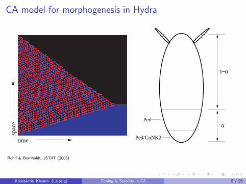
CA model for morphogenesis in Hydrasp

ace

time

Ped

Ped/CnNK2

α

1−α

rump

foot

Rohlf & Bornholdt, JSTAT (2005)


Seashell


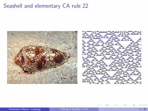
Seashell and elementary CA rule 22


Seashell and elementary CA rule 30


Role of noise?

Are the observed patterns robust under small stochasticperturbations?

Stability analysis in continuous dynamical systems: Make a smallperturbation and check if the system returns to the fixed point / limitcycle.

Here: Discretized state space. What is a “small” perturbation?

“Typical” implementation of noise in CA:

Stochastic asynchronous update


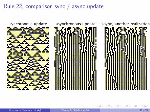
Rule 22, comparison sync / async update

synchronous update asynchronous update async, another realization


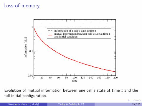
Loss of memory

0 20 40 60 80 100 120 140 160 180 200time

0.01

0.1

1in

form

atio

n [b

its]

information of a cell’s state at time tmutual information between cell’s state at time tand initial condition

Evolution of mutual information between one cell’s state at time t and thefull initial configuration.


Summary so far

Deterministic CA:“Complex” (interesting) spatio-temporal pattern formation

CA with noise implemented as stochastic update order:Largely irreproducible dynamics

Devastating effect of stochastic asynchronous update known for long,cf. Ingerson and Buvel, Physica D (1984)


How to proceed

Solution 0

Use more states and more complicated interactions to implementadditional clock signalscf. Nehaniv, Int. J. Alg. Comp. (2004)

Solution 1

Stick to simple rules

Consider a less destructive type of perturbation.

Get happy.


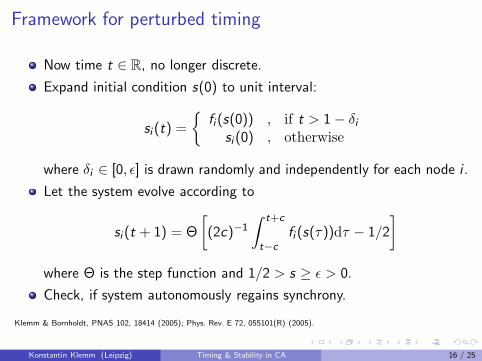
Framework for perturbed timing

Now time t ∈ R, no longer discrete.

Expand initial condition s(0) to unit interval:

si (t) =

{

fi(s(0)) , if t > 1 − δi

si (0) , otherwise

where δi ∈ [0, ǫ] is drawn randomly and independently for each node i .

Let the system evolve according to

si (t + 1) = Θ

[

(2c)−1

∫

t+c

t−c

fi (s(τ))dτ − 1/2

]

where Θ is the step function and 1/2 > s ≥ ǫ > 0.

Check, if system autonomously regains synchrony.

Klemm & Bornholdt, PNAS 102, 18414 (2005); Phys. Rev. E 72, 055101(R) (2005).


CA rule 22, initial timing perturbation


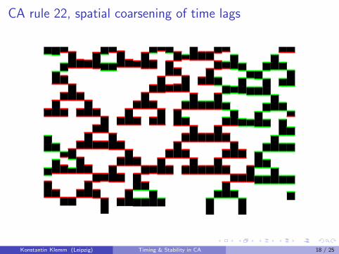
CA rule 22, spatial coarsening of time lags


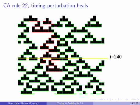
CA rule 22, timing perturbation heals

t=240


Probability of healing

0 200 400 600 8000

0.2

0.4

0.6

0.8

1

prob

. tha

t per

turb

atio

n he

als

out

CA rule 22

0 200 400 600 800number of cells N

CA rule 150

0 200 400 600 800

CA rule 110


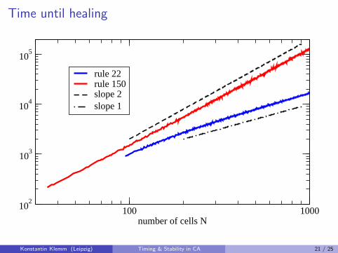
Time until healing

100 1000number of cells N

102

103

104

105

rule 22rule 150slope 2slope 1


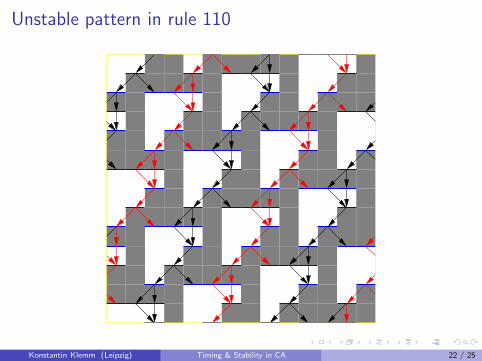
Unstable pattern in rule 110


Overview of results

stable elementary rules0, 4, 22, 32, 36, 54, 72, 76, 104, 128, 132, 160, 164, 200, 204, 218,222, 236, 250,254

partially stable el. rules (strong dependence on n)90, 122, 126, 150

unstable elementary rules50, 94, 108, 110, 178

Elementary CA fail to produce sustained synchronous blinking of allcells

Game of Life: Blinkers, gliders, spaceships etc. are unstable


Further results


Summary

Stable and unstable CA rules can be distinguished by theirresponse to minimal timing perturbations.


Download - Timing and stability in cellular automata - tbi.univie.ac.at · Timing and stability in cellular automata Konstantin Klemm Bioinformatics Group University of Leipzig, Germany Konstantin

Top Related