Automata

Summary

Deterministic Automata Languages

Stochastic Automata Other Automata Formalisms

Automata with input and output

Protocol Representation with Finite State Automata (FSM)

Timed Automata

Deterministic Automaton

X is the state space E is the event set associated with G f: XEX is the transition function

f(x,e)=y means that when G is at state x and event e occurs then G transitions to y

Γ is the feasible event set. For every state x, Γ(x) is the set of all events that are

active x0 is the initial state Xm is the set of marked states and is a subset of X

0, , , , , mG X E f x X

Example: Computer Basic Functions

Design an automaton that describes the basic functions of a computer: down, waiting, processing

State space D: down, I: Idle, B: Busy

Event set f: failure, r: repair, a: job arrival, c: job completion

Feasible event sets Γ(D)={r ,a}, Γ(I)={a, f}, Γ(B)={f, a, c} Alternatively Γ(I)={a} (computer cannot fail when idle)

Transition functions p(D, r)= I, p(D, a)=D p(I, a)= B, p(I, f)= D p(B, f)= D, p(B, a)= B, p(B, c)= I.

Initial state x0= I

Example: Automaton Graphical Representation

a

c

a

a

frf

I B

D

Languages Generated by Automata

a

c

a

a

fr

1 2

3

A language is a set of a finite length event strings to marked states

L={a, aa, aaa, …, ac, aac, aca, acaa, ar, aar, ara,…}

Example: Automaton Graphical Representation

a

c

a

a

ff

I B

D Now it is possible to

create a deadlock. D is an absorbing

state

Suppose that the technician has resigned and it is no longer possible to fix the computer.

Example: Queueing

What is an automaton model for simple FIFO queueing system?

State space X={0, 1, 2, 3, …}

Event set E={a, d} a: customer arrival, d: customer departure

Feasible event sets Γ(0)={a}, Γ(x)={a, d}, x > 0

Transition functions f(x, a)= x+1 f(x, d)= x-1, if x > 0

Initial state x0= 0

a d

State transition diagrama

d

a

d

a

d

a

d…0 1 2 3

Non-Deterministic Automaton

A non-deterministic automaton is similar to the deterministic except fnd: may probabilistically transition to a set of states. x0 the initial state may also be a set of states.

Example

0, , , , ,nd mG X E f x X

a

b

ba

1 2

3

Equivalent Deterministic Automaton

For each non-deterministic automaton there is an equivalent automaton that generates the same language.

a

b

ba

1 2

3

L={a, b, ab, ba. aba, bab, abab, baba, ababa, …}

a

b

ab

1 2

3

Automata with Inputs/Outputs

Each state “emits” an output symbol that is noted on the state

Alternatively, each transition is marked with the event that triggers the transition and below it lists the actions that are taken as a result of the transition.

1 2

3

a

c

bd

s1 s2

s3

1 2

3

a/s2

b/s2

c/s3d/s1

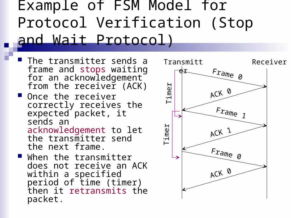
Example of FSM Model for Protocol Verification (Stop and Wait Protocol)

The transmitter sends a frame and stops waiting for an acknowledgement from the receiver (ACK)

Once the receiver correctly receives the expected packet, it sends an acknowledgement to let the transmitter send the next frame.

When the transmitter does not receive an ACK within a specified period of time (timer) then it retransmits the packet.

Tim

erT

imer

Transmitter ReceiverFrame 0

Frame 1

ACK 0

ACK 1

Frame 0

ACK 0

FSM for Stop and Wait Protocol

Transmitter

Ack 1 Received

Pkt 0 transmitted

Ack 0 ReceivedPkt 1

transmitted

Timeout or

Ack 0 Received

Timeout or

Ack 1 Received

Send Pkt 0

Send Pkt 1

Wait Ack 1 Wait Ack 0

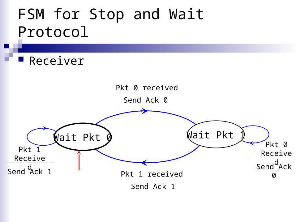
FSM for Stop and Wait Protocol

Receiver

Pkt 0 received

Send Ack 0

Pkt 1 received

Send Ack 1

Pkt 0 ReceivedPkt 1

Received

Wait Pkt 1Wait Pkt 0

Send Ack 1Send Ack 0

Timed Automata Models

So far, the models we studied did not consider the time when an event occurred.

For dynamic systems, the sample path of the system is specified by the sequence of pairs {(ei,ti)} where ei is the i-th event and ti is the time that the event has occurred.

Timed automata are similar to the deterministic automata with the addition of a clock structure

0, , , , ,G X E f x V V is the clock structure Xm (the set of marked states) is omitted for simplicity

Simple Example

Assume a system with a single event, i.e., E={a} and Γ(x)={a} for all xX. We are interested for the sequence {(ei, ti)} where ei is the i-th event and ti is the time when ei occurs.

t1

e1 = a

tk-1

ek-1 = a

tk

ek = a

t2

e2 = a…

t

time

vk

zk yk

vk= tk-tk-1 is the event lifetime

zk= t - tk-1 is the age of event

yk= tk - t is the residual lifetime

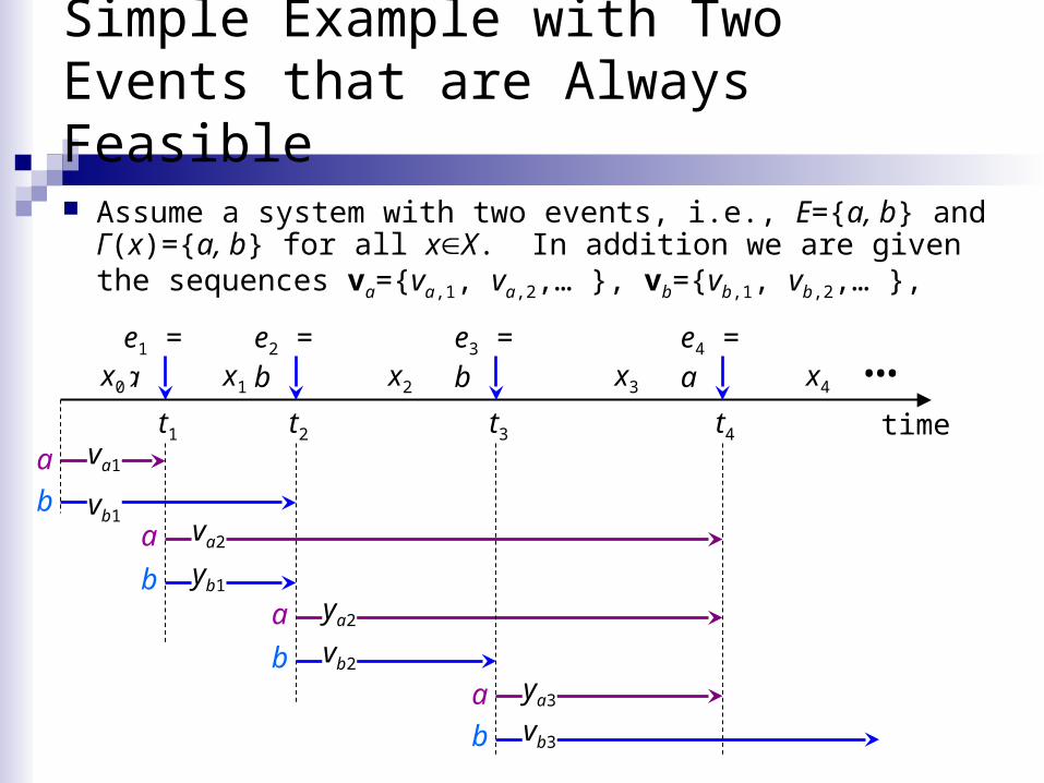
Simple Example with Two Events that are Always Feasible

Assume a system with two events, i.e., E={a, b} and Γ(x)={a, b} for all xX. In addition we are given the sequences va={va,1, va,2,… }, vb={vb,1, vb,2,… },

t1

e1 = a

timea

b

va1

vb1

a

b

va2

yb1

t2

e2 = b

a

b

ya2

vb2

t3

e3 = b

a

b

ya3

vb3

t4

e4 = ax0 x1 x2 x3 x4

…

Example with Two Events that are NOT Always Feasible

Assume that in the previous example that Γ(x)={a,b} for x{x0, x2, x4} Γ(x)={b} for x{x1 , x3,}

t1

e1 = a

timea

b

va1

vb1

b yb1

t2

e2 = b

a

b

va2

vb2

t3

e3 = b

a

b

ya2

vb3

t4

e4 = bx0 x1 x2 x3 x4

…

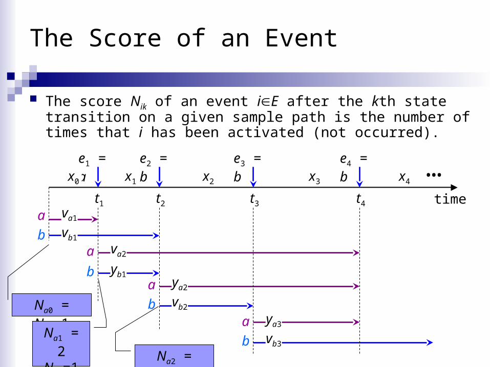
The Score of an Event

The score Nik of an event iE after the kth state transition on a given sample path is the number of times that i has been activated (not occurred).

t1

e1 = a

timea

b

va1

vb1

a

b

va2

yb1

t2

e2 = b

a

b

ya2

vb2

t3

e3 = b

a

b

ya3

vb3

t4

e4 = bx0 x1 x2 x3 x4

…

Na0 = Nb0=1

Na1 = 2Nb1=1 Na2 = Nb2=2

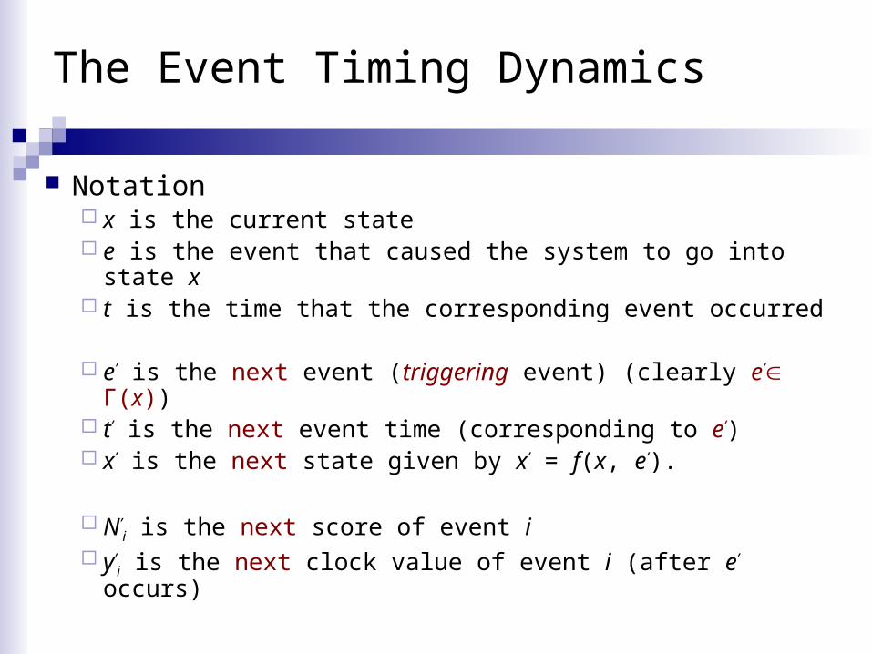
The Event Timing Dynamics

Notation x is the current state e is the event that caused the system to go into state x t is the time that the corresponding event occurred

e’ is the next event (triggering event) (clearly e’ Γ(x)) t’ is the next event time (corresponding to e’) x’ is the next state given by x’ = f(x, e’).

N’i is the next score of event i

y’i is the next clock value of event i (after e’ occurs)

The Event Timing Dynamics

Step 1: Given x evaluate the feasible event set Γ(x)

Step 2: From the clock value yi of all events i Γ(x) determine the minimum clock value

y*= miniΓ(x){yi}

Step 3: Determine the triggering event

e’= arg miniΓ(x){yi}

Step 4: Determine the next state

x’ = f(x, e’) where f() is the state transition function.

The Event Timing Dynamics

Step 5: Determine

t’= t + y*

Step 6: Determine the new clock values

Step 7: Determine the new event scores

*

, 1

if and ( ), ( )

if or ( )i

ii

i N

y y i e i xy i x

v i e i x

1 if or ( ), ( )

Otherwisei

ii

N i e i xN i x

N

State Space Model

The automaton timing dynamics can also be represented as a dynamical system

1

1

1

, , , ,...,

, , , ,...,

, , , ,...,

m

m

m

x f x y N v v

y g x y N v v

N h x y N v v

1 1,1 1,2, ,...v v v

2 2,1 2,2, ,...v v v

…

INPUT

1 1 2 2, , , ,...e t e t

OUTPUT

The initial conditions are given by x0, Ni,0=1 for all i Γ(x0) and Ni,0=0 for all i Γ(x0) and yi = vi,1 for all i Γ(x0).

What represents the state variables of the system?

Example: Queueing Model

State space X={0, 1, 2, 3, …}

Event set E={a, d} a: customer arrival, d: customer departure

Feasible event sets Γ(0)={a}, Γ(x)={a, d}, x > 0

Transition functions

Initial state x0= 0

a d

Clock structure Va ={0.5, 0.5, 1.0, 0.5, 2.0, 0.5, …} Vd ={1.0, 1.5, 0.5, 0.5, 1.0, …} In general, the numbers of the clock structure are generated by a

Random Number Generator

1 if ,

1 if

x e af x e

x e d

Example: Queueing Model

time

a

b

0.5

Clock structure Va={0.5, 0.5, 1.0, 0.5, 2.0, 0.5, …} Vd={1.0, 1.5, 0.5, 0.5, 1.0, …}

0.5

1 0.51.5

0.51 2

0.5

0.5

1

t=0 t=0.5 t=1 t=1.5 t=2 t=2.5 t=3 t=3.5 t=4 t=4.5 t=5

The Event Scheduling Scheme

INITIALIZE

EVENT CALENDAR

e1 t1

e2 t2…

CLOCK STRUCTURE

TIMESTATE

Update Statex’=f(x,e1)

Update Timet’=t1

Delete Infeasible

EventsAdd New Feasible Events

Recall the Queueing System from Introduction

System Input

2

1 if truck arrives at ( )

0 otherwise

tu t

1

1 if parcel arrives at ( )

0 otherwise

tu t

System Dynamics

1 2

1 2

( ) 1 if ( ) 1, ( ) 0,

( ) ( ) 1 if ( ) 0, ( ) 1

( ) otherwise

x t u t u t

x t x t u t u t

x t

t

u1(t)

t

u2(t)

t

x(t)

Time Driven vs. Event Driven Simulation Models

Time Driven Dynamics

1 2

1 2

( ) 1 if ( ) 1, ( ) 0,

( ) ( ) 1 if ( ) 0, ( ) 1

( ) otherwise

x t u t u t

x t x t u t u t

x t

Event Driven Dynamics

1 if ,

1 if

x e af x e

x e d

State is updated only at the occurrence of a discrete event

In this case, time is divided in intervals of length Δt, and the state is updated at every step

Example: Two Queues in Series

Determine the automaton that describes the following network where the B1 and B2 have finite capacities of 3 and 2 packets respectively (including the customer in the server)

When a customer departs from B1 when B2 is full, then the customer is lost!

B1 B2

State

x = [x1, x2] where xi denotes the number of customers in Bi

State space X={[x1, x2] : x1= 0,…,3, x2 = 0, 1, 2}

Event set E={a, d1, d2}

Feasible event sets Γ([0,0])= {a}, Γ([0, x])={a, d2} if x > 0, Γ([x, 0])= {a, d1} if x > 0, Γ([x1, x2])= {a, d1, d2} if x1 > 0 and x2 > 0.

Transition functions

Initial state x0= [0,0].

Example: Two Queues in Series

1 2 1 1 2[ , ], [ 1,min{ 1,2}]f x x d x x

a d2B1 B2d1

1 2 1 2[ , ], [min{ 1,3}, ]f x x a x x

1 2 2 1 2[ , ], [ , 1]f x x d x x

Communication Link

How would you model a transmission link that can transmit packets at a rate G packets per second and has a propagation delay equal to 100ms?

B1 B2

B1

…?

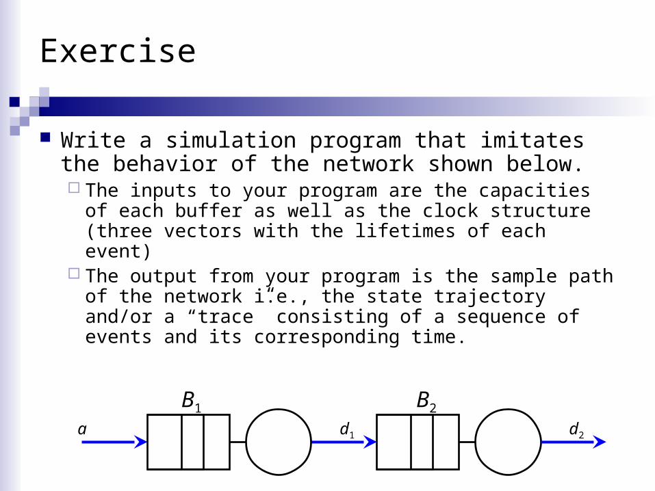
Exercise

Write a simulation program that imitates the behavior of the network shown below. The inputs to your program are the capacities of each

buffer as well as the clock structure (three vectors with the lifetimes of each event)

The output from your program is the sample path of the network i.e., the state trajectory and/or a “trace” consisting of a sequence of events and its corresponding time.

B1 B2

a d1 d2

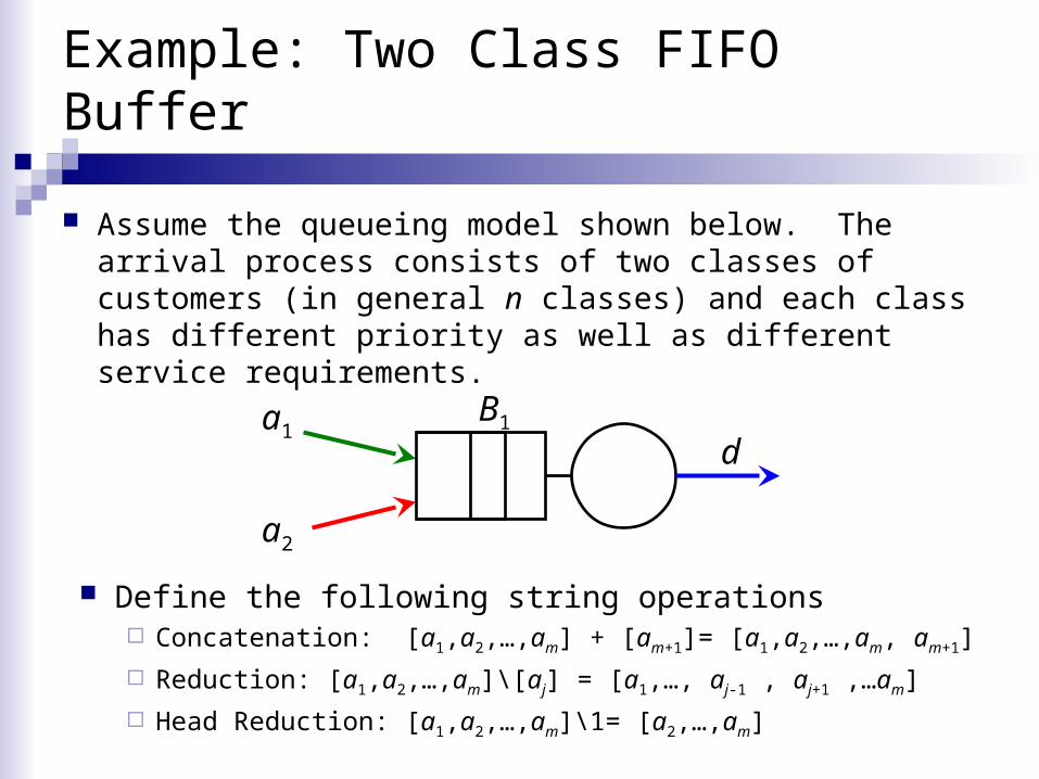
Example: Two Class FIFO Buffer

Assume the queueing model shown below. The arrival process consists of two classes of customers (in general n classes) and each class has different priority as well as different service requirements.

B1a1

a2

d

Define the following string operations Concatenation: [a1,a2,…,am] + [am+1]= [a1,a2,…,am, am+1]

Reduction: [a1,a2,…,am]\[aj] = [a1,…, aj-1 , aj+1 ,…am]

Head Reduction: [a1,a2,…,am]\1= [a2,…,am]

Example: Two Class FIFO Buffer

Event Set E={a1,a2, d}

State Space: X={ x : {ε} {all possible permutations of a1 and a2 with length

0,…,K}} K is the buffer size

Feasible Event set Γ(ε)={a1,a2} and Γ(x)={a1,a2,d} for all other states x

Transition Functions f(x, a1)= x + {a1}

f(x, a2)= x + {a2}

f(x, d)= x\1 for all x {ε}.

Initial State: x0 = ε.

Exercise

Consider the two class FIFO buffer from the previous example and determine how you would simulate the following policies

Threshold policy (with threshold B < K ) When a high priority customer arrives (e.g. a1), it is accommodated as

long as there is enough buffer space, i.e., as long as |x| < K where |x| is the “cardinality” of the set x, (the number of elements in x or 0 if x=ε).

When a low priority customer arrives (e.g. a2), it is accommodated only if the number of customers currently in the queue does not exceed B, i.e., as long as |x| < B.

Push-out Policy When a low priority customer arrives, it is accommodated if |x| < K. When a high priority customer arrives, it is accommodated at the end

of the queue if |x| < K. However, if |x| = K then, the last low priority customer from the queue (if one is present) is removed and the new customer is accommodated the at the tail of the queue.

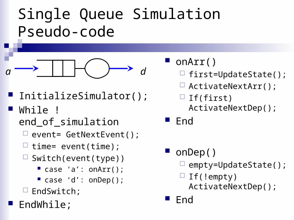
Single Queue Simulation Pseudo-code

InitializeSimulator(); While !end_of_simulation event= GetNextEvent(); time= event(time); Switch(event(type))

case ‘a’: onArr(); case ‘d’: onDep();

EndSwitch;

EndWhile;

a d onArr()

first=UpdateState(); ActivateNextArr(); If(first) ActivateNextDep();

End

onDep() empty=UpdateState(); If(!empty) ActivateNextDep();

End