
1
Solution Methods
Lecture 04
Steady State Diffusion Equation

Solution methods
• Focus on finite volume method.
• Background of finite volume method.
• Discretization example.
• General solution method.
• Convergence.
• Accuracy and numerical diffusion.
• Pressure velocity coupling.
• Segregated versus coupled solver methods.
• Multigrid solver.
• Summary.

Overview of numerical methods
• Many CFD techniques exist.
• The most common in commercially available CFD programs are:
• The finite volume method has the broadest applicability (~80%).
• Finite element (~15%).
• Here we will focus on the finite volume method.
• There are certainly many other approaches (5%), including:
• Finite difference method (FDM).
• Finite element method (FEM).
• Spectral method.
• Boundary element method (BEM).
• Vorticity based methods.
• Lattice gas/lattice Boltzmann.
• And more!

4
Finite difference method (FDM)
• Historically, the oldest of the three.
• Techniques published as early as 1910 by L. F. Richardson.
• Seminal paper by Courant, Fredrichson and Lewy (1928) derived
stability criteria for explicit time stepping.
• First ever numerical solution: flow over a circular cylinder by
Thom (1933).
• Scientific American article by Harlow and Fromm (1965) clearlyand publicly expresses the idea of “computer experiments” for the
first time and CFD is born!!
• Advantage: easy to implement.
• Disadvantages: restricted to simple grids and does not conserve
momentum, energy, and mass on coarse grids.

• The governing equations (in differential form) are
discretized (converted to algebraic form).
• First and second derivatives are approximated by
truncated Taylor series expansions.
• The resulting set of linear algebraic equations is
solved either iteratively or simultaneously.
Finite difference: basic methodology
• The domain is discretized into a series of grid points.
• A “structured” (ijk) mesh is required.

Subtract:
Taylor Series: central finite difference method
• Central difference formula• 2nd order accurate
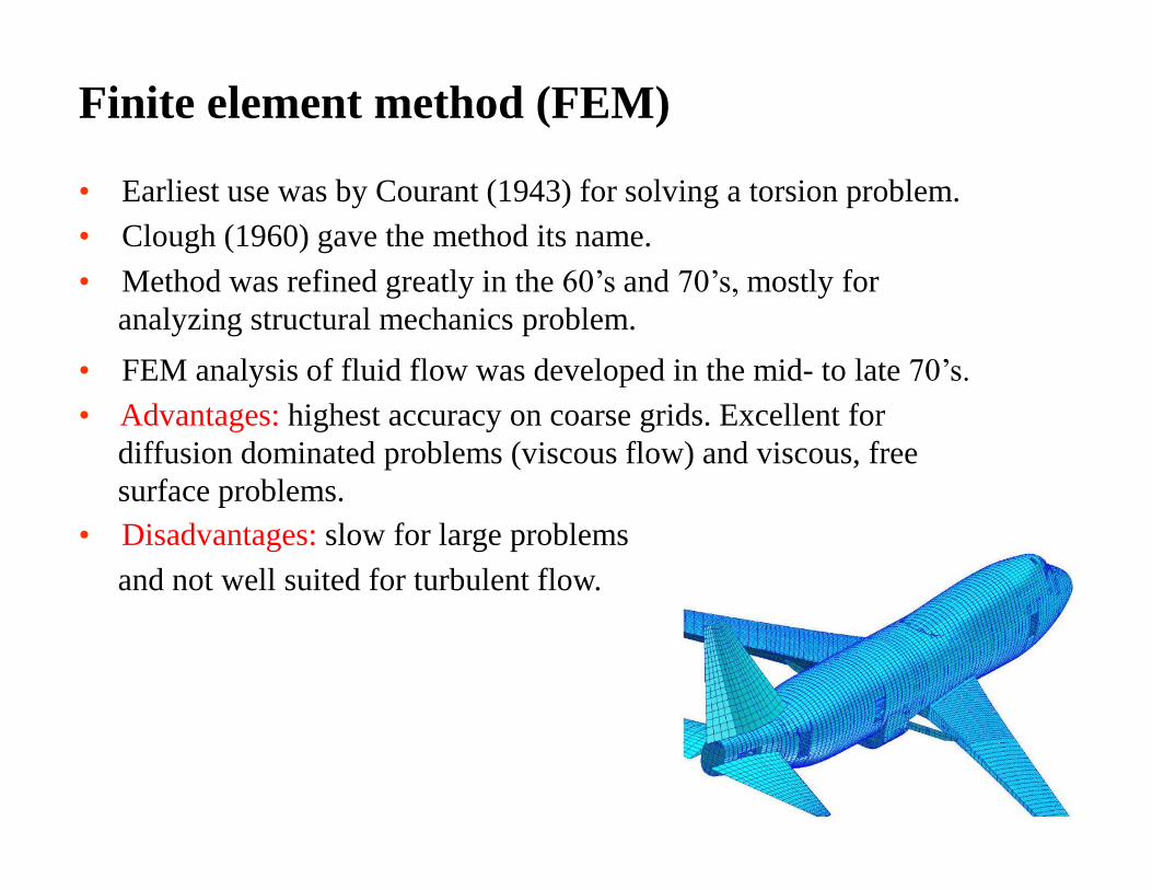
• Earliest use was by Courant (1943) for solving a torsion problem.
• Clough (1960) gave the method its name.
• Method was refined greatly in the 60’s and 70’s, mostly for
analyzing structural mechanics problem.
• FEM analysis of fluid flow was developed in the mid- to late 70’s.
• Advantages: highest accuracy on coarse grids. Excellent for
diffusion dominated problems (viscous flow) and viscous, free
surface problems.
• Disadvantages: slow for large problems
and not well suited for turbulent flow.
Finite element method (FEM)

7
• First well-documented use was by Evans and Harlow (1957) at Los
Alamos and Gentry, Martin and Daley (1966).
• Advantage: Was attractive because while variables may not be continuouslydifferentiable across shocks and other discontinuities; mass, momentum
and energy are always conserved.
• FVM enjoys an advantage in memory use and speed for very large
problems, higher speed flows, turbulent flows, and source term
dominated flows (like combustion).
• Late 70’s, early 80’s saw development of body-fitted grids. By early 90’s,
unstructured grid methods had appeared.
• Advantages: basic FV control volume balance does not limit cell shape;
mass, momentum, energy conserved even on coarse grids; efficient,
iterative solvers well developed.
• Disadvantages: false diffusion when simple numerics are used.
Finite volume method (FVM)

• Integrate the differential equation over the control volume and
apply the divergence theorem.
• To evaluate derivative terms, values at the control volume faces
are needed: have to make an assumption about how the value
varies.
• Result is a set of linear algebraic equations: one for each control
volume.
• Solve iteratively or simultaneously.
Finite volume: basic methodology
• Divide the domain into control volumes.

9
Cells and nodes
• Using finite volume method, the solution domain is subdivided
into a finite number of small control volumes (cells) by a grid.
• The grid defines the boundaries of the control volumes while the
computational node lies at the center of the control volume.
• The advantage of FVM is that the integral conservation is
satisfied exactly over the control volume.

10
Typical control volume
• The net flux through the control volume boundary is the sum of
integrals over the four control volume faces (six in 3D). The
control volumes do not overlap.
• The value of the integrand is not available at the control volume
faces and is determined by interpolation.

The Finite Volume Method for Diffusion Problems

• Consider the 1D diffusion (conduction)equation with source term S
Finite Volume method
Another form,
• where is the diffusion coefficient and S is the source term.
• Boundary values of at points A and B are prescribed.
• An example of this type of process, one-dimensional heat conduction in a
rod.

Step 1: Grid generation
• The first step in the finite volume method is to divide the domain into discrete control
volumes.
• Place a number of nodal points in the space between A and B. The boundaries (or faces)
of control volumes are positioned mid-way between adjacent nodes. Thus each node is
surrounded by a control volume or cell.
• It is common practice to set up control volumes near the edge of the domain in such a
way that the physical boundaries coincide with the control volume boundaries.
• A general nodal point is identified by P and its neighbours in a one-dimensional
geometry, the nodes to the west and east, are identified by W and E respectively.
• The west side face of the control volume is referred to by 'w' and the east side control
• volume face by ‘e’.
• The distances between the nodes W and P, and between nodes P and E, are identified by
xWP and xPE respectively. Similarly the distances between face w and point P and
between P and face e are denoted by xwP and xPe
• The control volume width is x = xwe

Step 2: Discretisation
• Integrate over the control volume, from west to east face
• The key step of the finite volume method is the integration of the governing equation(or equations) over a control volume to yield a discretised equation at its nodal pointP.
= 0
• Here A is the cross-sectional area of the control volume face, V is the volume and S is theaverage value of source S over the control volume. It is a very attractive feature of thefinite volume method that the discretised equation has a clear physical interpretation.
• Above equation states that the diffusive flux of leaving the east face minus the diffusiveflux of entering the west face is equal to the generation of , i.e. it constitutes abalance equation for over the control volume.

Step 2: Discretisation…
• In order to derive useful forms of the discretised equations, the interface diffusioncoefficient and the gradient d/dx at east (‘e’) and west ('w') are required.
• The values of the property and the diffusion coefficient are defined and evaluatedat nodal points.
• To calculate gradients (and hence fluxes) at the control volume faces an approximatedistribution of properties between nodal points is used. Linear approximations seem tobe the obvious and simplest way of calculating interface values and the gradients.
• This practice is called central differencing.• In a uniform grid linearly interpolated values for e and w are given by
• And the diffusive flux terms are evaluated as

• In practical situations, the source term S may be a function of the dependentvariable. In such cases the finite volume method approximates the source term bymeans of a linear form:
Step 2: Discretisation…
Therefore, equation become
Rearranging,
• Identifying the coefficients of W and E as AW and AE and the coefficient of P as AP , theabove equation can be written as
Where,
Discretised form of diffusionequation
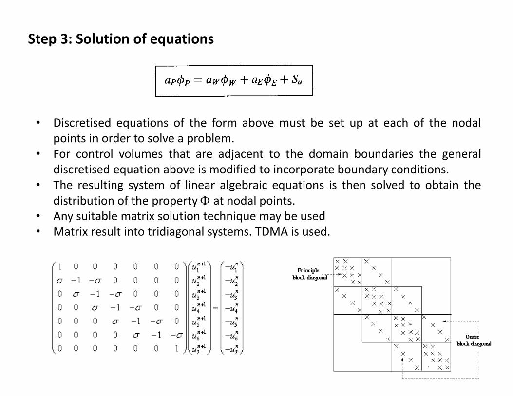
Step 3: Solution of equations
• Discretised equations of the form above must be set up at each of the nodalpoints in order to solve a problem.
• For control volumes that are adjacent to the domain boundaries the generaldiscretised equation above is modified to incorporate boundary conditions.
• The resulting system of linear algebraic equations is then solved to obtain thedistribution of the property at nodal points.
• Any suitable matrix solution technique may be used• Matrix result into tridiagonal systems. TDMA is used.
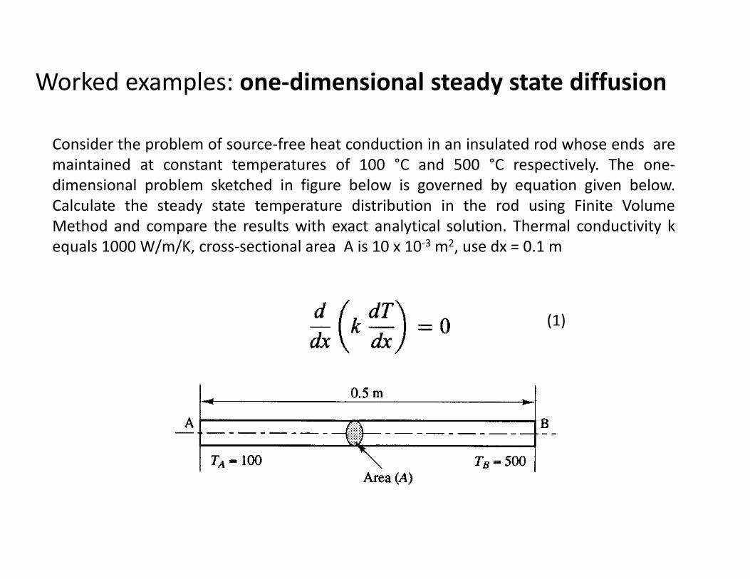
Worked examples: one-dimensional steady state diffusion
Consider the problem of source-free heat conduction in an insulated rod whose ends aremaintained at constant temperatures of 100 °C and 500 °C respectively. The one-dimensional problem sketched in figure below is governed by equation given below.Calculate the steady state temperature distribution in the rod using Finite VolumeMethod and compare the results with exact analytical solution. Thermal conductivity kequals 1000 W/m/K, cross-sectional area A is 10 x 10-3 m2, use dx = 0.1 m
(1)

Solution
• Divide the length of the rod into five equal control volumes as shown in Figurebelow. This gives dx = 0.1 m.
• The grid consists of five nodes. For each one of nodes 2, 3 and 4 temperature values tothe east and west are available as nodal values.
• Consequently, discretised equations can be readily written for control volumessurrounding these nodes:
• The thermal conductivity (ke = kw = k), node spacing (x) and cross-sectional area (Ae =AW = A) are constants. Therefore the discretised equation for nodal points 2, 3 and 4 is

With,
Solution…
• SU and SP are zero in this case since there is no source term in the governing equation
• Nodes 1 and 5 are boundary nodes, and therefore require special attention.Integration of equation (1) over the control volume surrounding point 1 gives
Re-arrange,
(2)
(3)

• Comparing equation 3 with equation 4 it can be easily identified that the fixedtemperature boundary condition enters the calculation as a source term (SU + SPTP) withSU = (2kA/x)TA and Sp = -2kA/x and that the link to the (west) boundary side has beensuppressed by setting coefficient aW to zero.
(4)
(3)
Solution…
• Equation 3 may be cast in the same linear form to yield the discretised equation forboundary node 1:
With,

• The control volume surrounding node 5 can be treated in a similar manner. Itsdiscretised equation is given by
Solution…
Re-arrange,
• The discretised equation for boundary node 5 is
Where,

• The discretisation process has yielded one equation for each of the nodal points 1 to 5.• Substitution of numerical values gives kA/x = 100 and the coefficients of each discretised
equation can easily be worked out. Their values are given in Table
Solution…
• The resulting set of algebraic equations for this example is

This set of equations can be re-arranged as
Solution…
• For TA = 100 and TB = 500 the solution can obtained by using, for example,Gaussian elimination:
• The exact solution is a linear distribution between the specified boundarytemperatures: T = 800x + 100. Figure shows that the exact solution and thenumerical results coincide.

Solution…

Assignment 5
Figure shows a large plate of thickness L = 2 cm with constant thermal conductivity k = 0.5W/m/K and uniform heat generation q = 1000 kW/m3 . The faces A and B are at temperatures of100 °C and 200 °C respectively. Assuming that the dimensions in the y- and z-directions are solarge that temperature gradients are significant in the x-direction only, calculate the steady statetemperature distribution using Finite volume Method. Compare the numerical result with theanalytical solution. The governing equation is
Page 92, CFD Book by Versteeg
1. Solve for 5, 10 and 15 nodes2. Compare the results
Heat conduction with source term

Assignment 6
Shown in Figure below is a cylindrical fin with uniform cross-sectional area A. The base is ata temperature of 100 °C (Tb) and the end is insulated. The fin is exposed to an ambienttemperature of 20 °C. One-dimensional heat transfer in this situation is governed by
where h is the convective heat transfer coefficient, P the perimeter, k the thermalconductivity of the material and T the ambient temperature. Calculate the temperaturedistribution along the fin and compare the results with the analytical solution given by
where n2 = hP/(kA), L is the length of the fin and x the distance along the fin. Data:L = 1 m, hP/{kA) = 25 m-2 (note kA is constant).
• Solve for 5, 10 and 15 nodes• Compare the results

Finite volume method for two-dimensionaldiffusion problems
• The methodology used in deriving discretised equations in the one-dimensionalcase can be easily extended to two-dimensional problems.
Two-dimensional grid used for the discretisation

• When the above equation is integrated over the control volume we obtain
• As before this equation represents the balance of the generation of in a control volumeand the fluxes through its cell faces.
• Using the approximations we can write expressions for the flux through control volumefaces:
(5)
Finite volume method for two-dimensional diffusion problems…
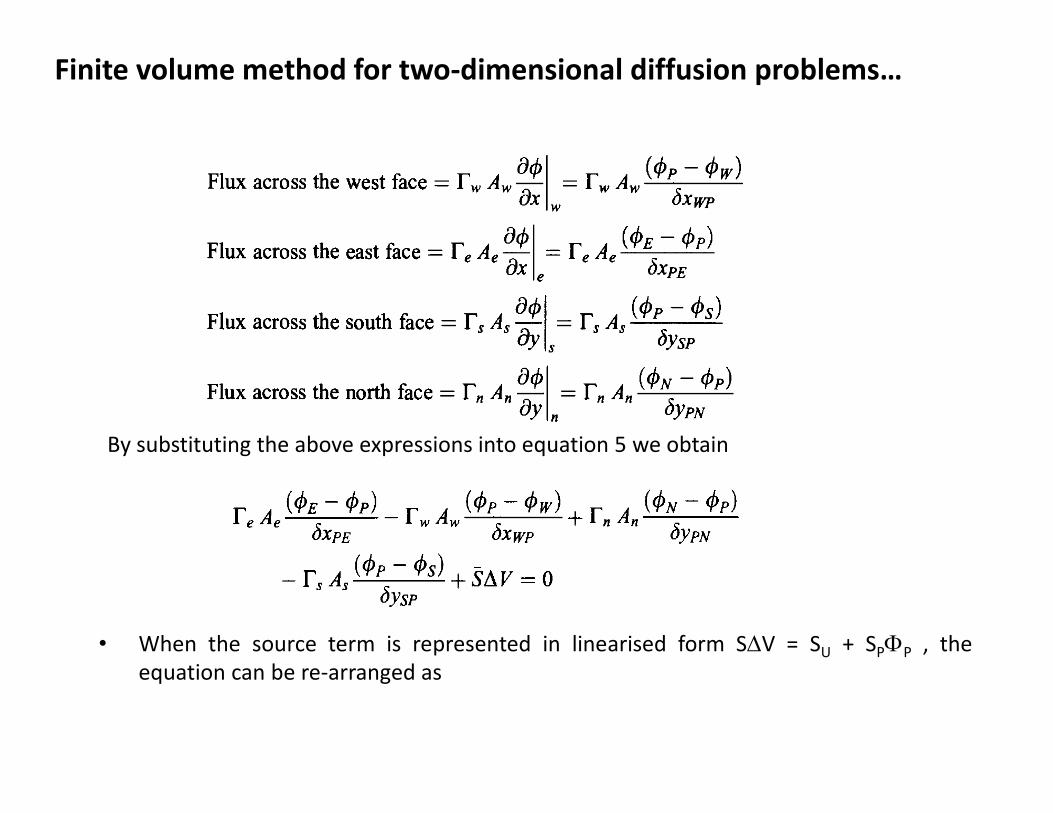
By substituting the above expressions into equation 5 we obtain
• When the source term is represented in linearised form SV = SU + SPP , theequation can be re-arranged as
Finite volume method for two-dimensional diffusion problems…

• Above equation is now cast in the general discretised equation form for interior nodes:
Where,
Finite volume method for two-dimensional diffusion problems…

• We obtain the distribution of the property in a given two-dimensionalsituation by writing above discretised equations at each grid node of thesubdivided domain.
• At the boundaries where the temperatures or fluxes are known the discretisedequations are modified to incorporate boundary conditions.
• The boundary side coefficient is set to zero (cutting the link with theboundary) and the flux crossing the boundary is introduced as a source whichis appended to any existing SU and SP terms.
• Subsequently, the resulting set of equations is solved to obtain the two-dimensional distribution of the property .
Finite volume method for two-dimensional diffusion problems…

Finite volume method for three-dimensionaldiffusion problems
• Steady state diffusion in a three-dimensional situation is governed by
A cell or control volume in three dimensions and neighboring nodes

• Integration of equation above over the control volume shown gives
• Putting the values at control faces (as in 2D case), we have
Finite volume method for three-dimensional diffusion problems…

Rearranging the coefficients, we have:
where
• Boundary conditions can be introduced by cutting links with the appropriateface(s) and modifying the source term as described earlier
Finite volume method for three-dimensional diffusion problems…

General approach
• In the previous example we saw how the species transport
equation could be discretized as a linear equation that can be
solved iteratively for all cells in the domain.
• This is the general approach to solving partial differential
equations used in CFD. It is done for all conserved variables
(momentum, species, energy, etc.).
• For the conservation equation for variable φ, the following steps
are taken:
– Integration of conservation equation in each cell.
– Calculation of face values in terms of cell-centered values.
– Collection of like terms.
• The result is the following discretization equation (with nb
denoting cell neighbors of cell P):

Guiding Principles
• Freedom of choice gives rise to a variety of discretization.
• As the number of grid points increased, all formulations areexpected to give the same solution.
• However, an additional requirements is imposed that willenable us to narrow down the number of acceptableformulations.
• We shall require that even the coarse grid solution shouldalways have Physically realistic behavior Overall balance

• Physically realistic behavior A realistic behavior should have the same qualitative trend as the exact
variation Example: In heat conduction without source no temperature can lie
outside the range of temperature established by the boundarytemperature
• Conservation The requirement of overall balance implies integral conservation over the
whole calculation domain – heat flux, mass flow rates, momentum fluxesmust correctly be balanced in overall for any grid size- not just for a finergrid
• Constraint Constraint of physical realism and overall balance will be used to guide our
choices of profile assumptions and related practices-on the basis of thesepractice we will develop some basic rule that will enable us to discriminatebetween available formulations and to invent new ones
Guiding Principles…

Four Basic Rules-(1/4)
• Consistency at control volume faces-same fluxexpression at the faces common to neighboring CVs

Four Basic Rules-(2/4)
• All coefficients must have same sign say positive. Implies that if neighbor goes up, P also goes up
• If an increase in E must lead to an increase in P , it follows that aE and aP
must have same sign

• But there are numerous formulations that frequentlyviolates this rule. Usually, the consequence is aphysically unrealistic solution.
• The presence of a negative neighbor coefficient canlead to the situation in which an increase in aboundary temperature causes the temperature at theadjacent grid point to decrease.
Four Basic Rules-(2/4)

Four Basic Rules-(3/4)

Four Basic Rules-(4/4)

Four Basic Rules-(4/4)

End


