rstaroyalsocietypublishingorg
ResearchCite this article Heywood KJ et al 2014Ocean processes at the Antarctic continentalslope Phil Trans R Soc A 372 20130047httpdxdoiorg101098rsta20130047
One contribution of 12 to a Theo MurphyMeeting Issue lsquoNewmodels and observationsof the Southern Ocean its role in globalclimate and the carbon cyclersquo
Subject Areasoceanography
KeywordsAntarctic continental shelf Antarctic SlopeFront ocean glider water mass climatemodel iron fertilization
Author for correspondenceKaren J Heywoode-mail kheywoodueaacuk
Ocean processes at theAntarctic continental slopeKaren J Heywood1 Sunke Schmidtko1 Ceacuteline Heuzeacute1
Jan Kaiser1 Timothy D Jickells1 Bastien Y Queste1
David P Stevens2 Martin Wadley2
Andrew F Thompson3 Sophie Fielding4
Damien Guihen4 Elizabeth Creed5 Jeff K Ridley6
and Walker Smith7
1Centre for Ocean and Atmospheric Sciences School ofEnvironmental Sciences and 2Centre for Ocean and AtmosphericSciences School of Mathematics University of East AngliaNorwich NR4 7TJ UK3California Institute of Technology Pasadena CA 91125 USA4British Antarctic Survey Cambridge CB3 0ET UK5Kongsberg Underwater Technology Inc LynnwoodWA 98036 USA6Met Office Hadley Centre Exeter EX1 3PB UK7Virginia Institute for Marine Science College of William and MaryGloucester Point VA 23062 USA
The Antarctic continental shelves and slopes occupyrelatively small areas but nevertheless are importantfor global climate biogeochemical cycling andecosystem functioning Processes of water masstransformation through sea ice formationmeltingand oceanndashatmosphere interaction are key to theformation of deep and bottom waters as well asdetermining the heat flux beneath ice shelves Climatemodels however struggle to capture these physicalprocesses and are unable to reproduce water massproperties of the region Dynamics at the continentalslope are key for correctly modelling climate yettheir small spatial scale presents challenges bothfor ocean modelling and for observational studiesCross-slope exchange processes are also vital for theflux of nutrients such as iron from the continentalshelf into the mixed layer of the Southern Ocean An
2014 The Authors Published by the Royal Society under the terms of theCreative Commons Attribution License httpcreativecommonsorglicensesby30 which permits unrestricted use provided the original author andsource are credited
on January 29 2018httprstaroyalsocietypublishingorgDownloaded from
2
rstaroyalsocietypublishingorgPhilTransRSocA37220130047
iron-cycling model embedded in an eddy-permitting ocean model reveals the importance ofsedimentary iron in fertilizing parts of the Southern Ocean Ocean gliders play a key role inimproving our ability to observe and understand these small-scale processes at the continentalshelf break The Gliders Excellent New Tools for Observing the Ocean (GENTOO) projectdeployed three Seagliders for up to two months in early 2012 to sample the water to the east ofthe Antarctic Peninsula in unprecedented temporal and spatial detail The glider data resolvesmall-scale exchange processes across the shelf-break front (the Antarctic Slope Front) and thefrontrsquos biogeochemical signature GENTOO demonstrated the capability of ocean gliders toplay a key role in a future multi-disciplinary Southern Ocean observing system
1 IntroductionThe Antarctic continental shelf and slope are often considered outposts of ocean research they areremote covered in sea ice for much of the year and small in geographical extent Mostly poorlymapped these shallow regions host counter-currents to the largest current on the planet theAntarctic Circumpolar Current (ACC) Observational studies are mostly restricted to the summermonths whereas Argo floats operating year-round typically provide few profiles south of theACC Here we discuss several areas of science that illustrate the importance of the Antarctic shelfand slope and the need for further observational and model investigations
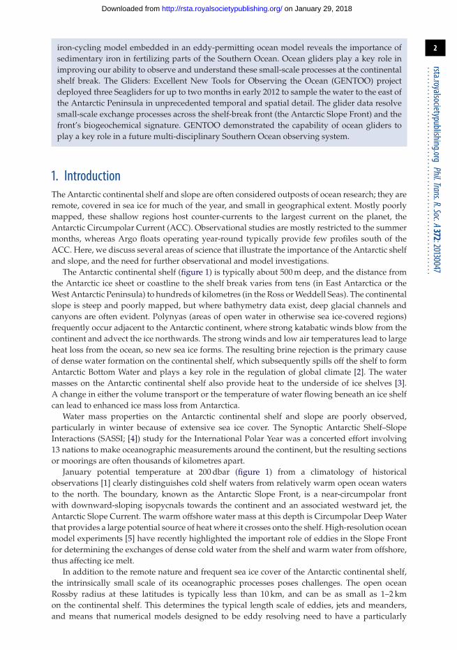
The Antarctic continental shelf (figure 1) is typically about 500 m deep and the distance fromthe Antarctic ice sheet or coastline to the shelf break varies from tens (in East Antarctica or theWest Antarctic Peninsula) to hundreds of kilometres (in the Ross or Weddell Seas) The continentalslope is steep and poorly mapped but where bathymetry data exist deep glacial channels andcanyons are often evident Polynyas (areas of open water in otherwise sea ice-covered regions)frequently occur adjacent to the Antarctic continent where strong katabatic winds blow from thecontinent and advect the ice northwards The strong winds and low air temperatures lead to largeheat loss from the ocean so new sea ice forms The resulting brine rejection is the primary causeof dense water formation on the continental shelf which subsequently spills off the shelf to formAntarctic Bottom Water and plays a key role in the regulation of global climate [2] The watermasses on the Antarctic continental shelf also provide heat to the underside of ice shelves [3]A change in either the volume transport or the temperature of water flowing beneath an ice shelfcan lead to enhanced ice mass loss from Antarctica
Water mass properties on the Antarctic continental shelf and slope are poorly observedparticularly in winter because of extensive sea ice cover The Synoptic Antarctic ShelfndashSlopeInteractions (SASSI [4]) study for the International Polar Year was a concerted effort involving13 nations to make oceanographic measurements around the continent but the resulting sectionsor moorings are often thousands of kilometres apart
January potential temperature at 200 dbar (figure 1) from a climatology of historicalobservations [1] clearly distinguishes cold shelf waters from relatively warm open ocean watersto the north The boundary known as the Antarctic Slope Front is a near-circumpolar frontwith downward-sloping isopycnals towards the continent and an associated westward jet theAntarctic Slope Current The warm offshore water mass at this depth is Circumpolar Deep Waterthat provides a large potential source of heat where it crosses onto the shelf High-resolution oceanmodel experiments [5] have recently highlighted the important role of eddies in the Slope Frontfor determining the exchanges of dense cold water from the shelf and warm water from offshorethus affecting ice melt
In addition to the remote nature and frequent sea ice cover of the Antarctic continental shelfthe intrinsically small scale of its oceanographic processes poses challenges The open oceanRossby radius at these latitudes is typically less than 10 km and can be as small as 1ndash2 kmon the continental shelf This determines the typical length scale of eddies jets and meandersand means that numerical models designed to be eddy resolving need to have a particularly
on January 29 2018httprstaroyalsocietypublishingorgDownloaded from
3
rstaroyalsocietypublishingorgPhilTransRSocA37220130047
180deg W
60degW
60deg E
60deg S
70deg S 64deg S
63deg S
62deg S
61deg S
60deg S
(a) (b)
58deg W
ndash7000 ndash6000 ndash5000 ndash4000
depth (m)
cons
erva
tive
tem
pera
ture
(degC
)
ndash3000 ndash2000 ndash1000 0
56deg W 54deg W 52deg W 50deg W 48deg W 46deg W
0deg30 SG539
SG522SG546sea ice 23 Jansea ice 24 Mar
25
20
15
10
05
0
ndash05
ndash10
ndash15
80deg S
120deg
E120degW
Figure 1 (a) Map of Antarctica showing the conservative temperature at 200 dbar from the MIMOC climatology for the monthof January [1] Bathymetric contours (grey lines) are shown at 1000 2000 and 3000 m to indicate the location of the Antarcticcontinental slope Black box indicates the GENTOO study area shown expanded (b) with the three glider tracks SeaglidersTashtego (SG539 red) and Beluga (SG522 green) were deployed at approximately the same time (January) and location atapproximately 635 S 53 W Seaglider Flying Pig (SG546 orange) was deployed twoweeks later in the Powell Basin to surveythe continental slope of the South Orkney Islands Cyan line indicates the sea ice edge (15 concentration) at the beginning ofthe glider deployment and blue line indicates the ice edge when Tashtego was recovered in March
high resolution and that observations across the continental shelf and slope need to beclosely spaced
2 Representation of Antarctic shelf and slope processes in climate modelsThe processes on the Antarctic continental shelf and slope are important for global climate andbiogeochemical cycles but steep bathymetry small spatial scale of fronts and eddies and complexinteractions between atmosphere sea ice meteoric ice and water masses combine to make thisregion particularly challenging for climate models Considerable efforts are being expended atclimate modelling centres worldwide to address these issues Can the latest generation of climatemodels adequately represent the water masses around Antarctica
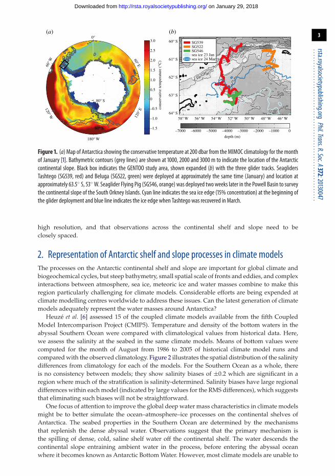
Heuzeacute et al [6] assessed 15 of the coupled climate models available from the fifth CoupledModel Intercomparison Project (CMIP5) Temperature and density of the bottom waters in theabyssal Southern Ocean were compared with climatological values from historical data Herewe assess the salinity at the seabed in the same climate models Means of bottom values werecomputed for the month of August from 1986 to 2005 of historical climate model runs andcompared with the observed climatology Figure 2 illustrates the spatial distribution of the salinitydifferences from climatology for each of the models For the Southern Ocean as a whole thereis no consistency between models they show salinity biases of plusmn02 which are significant in aregion where much of the stratification is salinity-determined Salinity biases have large regionaldifferences within each model (indicated by large values for the RMS differences) which suggeststhat eliminating such biases will not be straightforward
One focus of attention to improve the global deep water mass characteristics in climate modelsmight be to better simulate the oceanndashatmospherendashice processes on the continental shelves ofAntarctica The seabed properties in the Southern Ocean are determined by the mechanismsthat replenish the dense abyssal water Observations suggest that the primary mechanism isthe spilling of dense cold saline shelf water off the continental shelf The water descends thecontinental slope entraining ambient water in the process before entering the abyssal oceanwhere it becomes known as Antarctic Bottom Water However most climate models are unable to
on January 29 2018httprstaroyalsocietypublishingorgDownloaded from
4
rstaroyalsocietypublishingorgPhilTransRSocA37220130047
(a)
clim CanESM2 CNRM-CM5CSIRO
Mk3-6-0017 017017
obs
GFDLESM2M
010
009
016069 024
MIROC4h MIROCESM-CHEM
021
INMCM4GFDL
ESM2G
026 009010
NorESM1MMRICGCM3
MPIIPSLCM5A-LR ESM-LR
013 008 009HadGEM2-ES HiGEMGISS-E2-R
(e)
(i)
(m) (n)
3460 3464 3468 3472 3476 3480 ndash02 ndash01 0 01 02
(o) ( p)
( j) (k) (l)
(g) (h)( f )
(b) (c) (d )
Figure 2 Mean bottom practical salinity of theWorld Ocean Circulation Experiment (WOCE) climatology (a) andmean bottomsalinity difference (model-climatology) (bndashp) for a selection of 15 CMIP5 climate models for winter (August) 20 year meanLeft colour bar corresponds to the climatology right colour bar to the differences model-climatology Numbers indicate area-weighted root mean square differences (RMSD) for all depths between the model and the climatology Mean RMSD is 018
simulate this formation process The lsquosuccessfulrsquo models (in terms of their representation of oceanproperties in the abyssal ocean) are those that form dense water by open ocean deep convection[6] thus incorrectly representing key processes We now consider separately the salinity of thewaters on the Antarctic continental shelf and in the abyss (figures 2 and 3) to shed light onthese processes
Figure 3ab summarizes for all models the area-weighted mean bottom temperature andbottom salinity differences (model minus observations) for the deep Southern Ocean (bathymetricdepth greater than 2000 m) and the Antarctic shelves (bathymetric depth less than 2000 m) Foreach domain we remove these biases prior to calculating the root mean square (RMS) differencesshown in figure 3cd Models exhibiting very different RMS and mean differences are those withhighly spatially variable biases More than half of the models exhibit a fresh bias on the shelf andslope Some models demonstrate a fresh bias but with very localized saline biases resulting inaverage high-density biases on the shelf These localized highly saline and dense water massesmay be able to sporadically escape the continental shelf and contribute to replenishing the
on January 29 2018httprstaroyalsocietypublishingorgDownloaded from
5
rstaroyalsocietypublishingorgPhilTransRSocA37220130047
0
11
10
15
20
3
5
1 3 5 73 5RMS salinity difference times10ndash4 RMS salinity difference times10ndash4
times10ndash3 times10ndash3
RM
S te
mpe
ratu
re d
iffe
renc
e (deg
C)
7 9
ndash02ndash1
0
1
2
02
mean salinity difference
mea
n te
mpe
ratu
re d
iffe
renc
e (deg
C)
04 06 ndash02
(a)
(c) (d )
(b)
ndash03
ndash05
0
05
10
ndash01
mean salinity difference
0 01 02
CanESM2
CNRM-CM5
GFDL-ESM2M
GISS-E2-R
HiGEM
IPSL-CM5A-LR
MPI-ESM-LR
MRI-CGCM3
NorESM1-M
GFDL-ESM2G
MIROC4h
MIROC-ESM-CHEM
inmcm4
HadGEM2-ES
CSIRO-Mk3-6-0
Figure 3 Area-weighted mean (ab) and root mean square (cd) property differences for each climate model compared withclimatology (model minus observations) for the deep Southern Ocean (ac bathymetric depth greater than 2000 m) and theshelves (bd bathymetric depth less than 2000 m) The RMS differences have been calculated after first removing the meanbias for each model Z-level models have square symbols the isopycnal coordinate model a triangle and the sigma coordinatemodels have circles All calculations are for the Southern Ocean between 80 S and 50 S
Antarctic Bottom Water but such an intermittent process is difficult to detect in monthly climatemodel output This localized formation of dense water could be a very effective way in whicha climate model could replenish the abyss even if it is not accurately simulating the processesoccurring in the real ocean
In general the models that have large temperature or salinity biases in the abyss also have largebiases on the continental shelf models mostly (although not always) lie in the same quadrants infigure 3ab There are no significant differences between the numbers of models in each of thefour quadrants biases are seemingly random Models that have larger temperature biases do notnecessarily have large salinity biases and vice versa Models can have large mean biases butsmall de-biased RMS differences indicating that the whole of the Southern Ocean is uniformlybiased in those models There is no apparent relationship between model fidelity and coordinatescheme or resolution (the bottom row of models in figure 2 are sigma or isopycnal coordinatemodels and the others are z-coordinate models the coordinate systems are indicated by differentsymbols in figure 3) The lack of any particular patterns in the characteristics of the models infigure 3 confirms that improving deep water mass characteristics is not likely to require the samesolution in any two models the interplay of the climate model components is too complex
The model output in figure 2 represents winter conditions when the sea ice is at a maximumand salinity on the Antarctic continental shelf might be expected to be high The climatology(figure 2a) is biased towards summer observations when ice is melting We might expect aseasonal saline bias in the modelled water masses at the seabed on the continental shelveshowever this would be associated with a cold bias Too saline water masses on the continentalshelf may be a result of too much sea ice formation in the models generating large amounts ofbrine that sinks to the seabed
on January 29 2018httprstaroyalsocietypublishingorgDownloaded from
6
rstaroyalsocietypublishingorgPhilTransRSocA37220130047
The properties of the water masses on the Antarctic continental shelf are poorly simulatedbut there is no consistent behaviour in the models studied in the formation of either dense shelfwater or abyssal water Some simulations are too fresh and others too saline and the biases on theshelf are not always the same in the deep Southern Ocean Some models probably produce densewater through unrealistic processes Does it matter that climate models are unable to representthese water masses It does especially if we need to accurately predict likely future melt ratesand stability of Antarctic ice shelves and ice sheets because the relatively warm ocean providesthe heat source for ice shelf basal melt If the climate models form too much thick sea ice that isnot advected away then this prevents heat from leaving the ocean [7] The formation of AntarcticBottom Water is a crucial part of the coupled climate system yet the climate models are unable toboth create and export water of correct characteristics
Coastal and open ocean polynyas are one of the processes that need to be better representedin climate models Although they have a relatively small geographical extent compared with sea-ice-covered regions polynyas are the sites of the most rapid and extensive changes in water massproperties through loss of heat to the atmosphere and brine rejection through sea ice formationThe next-generation climate models are evaluating ice shelf cavities [8] which may improve theshelf water properties However the fundamental problem of continental shelf edge flows can beresolved only with high horizontal and vertical resolution Even global model resolutions of 112are insufficient to be eddy permitting at high latitudes so alternative techniques may be requiredSuch methods include two-way embedded high-resolution models [9] or targeted irregular meshmodels [10]
3 Seaglider observations of Antarctic processes on the shelf and slopeThe complexity and small spatial scale of the processes on the Antarctic continental shelfand slope are not only a challenge for numerical models but they also pose a challenge forobservational oceanography and in the design of the Southern Ocean Observing System (SOOS)Regional and idealized models have suggested that the space and time scales of variability onthe Antarctic margin may be as small as O(1 km) and a couple of days [51112] These scalesare not amenable to study by ship or moorings One emerging technology is the ocean glider anautonomous underwater vehicle (AUV) able to profile the ocean for months at a time [13] Withouta propeller gliders are more energy efficient than other AUVs and data can be transmitted backto the user each time the glider surfaces (typically every 4 h for dives to 1000 m depth with divesseparated horizontally by a few kilometres) This is a great advantage in a region that is bothinaccessible for ships and covered with sea ice that can advance or break up unpredictably withindays the loss of a glider does not mean the loss of the entire dataset
Gliders can carry a range of sensors to equip them for the interdisciplinary challenges ofthe twenty-first century The standard sensors presently include temperature salinity dissolvedoxygen chlorophyll fluorescence and optical backscatter Recently developed sensors includephotosynthetically active radiation acoustic backscatter for zooplanktonmicronekton p(CO2)and pH Considerable effort is being expended worldwide to design and develop smalllightweight sensors that do not have a large energy requirement particularly for biogeochemistryand ecology In addition gliders are being deployed in ever more challenging environments suchas beneath seasonal ice cover using acoustic navigation [14]
Recently gliders have begun to be used in polar regions we discuss one such deploymentto highlight the insights that may be gained particularly at the Antarctic shelf break In January2012 three Seagliders were deployed to the east of the tip of the Antarctic Peninsula (figure 1)as part of the Gliders Excellent New Tools for Observing the Ocean (GENTOO) project The goalwas to survey the continental shelf and slope of the Weddell Sea to assess the spatial and temporalvariability of the water masses and the Slope Front Extensive sea ice in early 2012 meant that themajority of the Seaglider sections crossed the slope in the Powell Basin and progressed graduallynorthward for recovery in March
on January 29 2018httprstaroyalsocietypublishingorgDownloaded from
7
rstaroyalsocietypublishingorgPhilTransRSocA37220130047
0
0
200
(a) (b)
400
600
800
10005 10 15 20 25
distance (km)
pres
sure
(db
ar)
Seaglider ship
30 35 40 45 50 0 5 10 15 20 25distance (km)
cons
tem
pera
ture
(degC
)
30 35 40 45 50ndash2
ndash1
0
1
Figure 4 Comparison of near-simultaneous glider (a) and ship-based (b) conservative temperature sections across theAntarctic continental slope into the Weddell Sea Locations of surface measurements are indicated by the black diamonds onthe upper axis Bathymetry is shown in grey Potential density contours are shown every 01 kg mminus3 as black lines
Comparing the southernmost Seaglider section with a relatively closely-spaced ship-basedconductivityndashtemperaturendashdepth (CTD) section (figure 4) occupied at the same time theadditional small-scale structure seen by the glider is apparent A CTD station spacing of 10 kmwhich would typically resolve the submesoscale structure in mid-latitudes is problematic atthis latitude There is a suggestion of some cold water in the core of the Slope Front (40 kmalong the section at approx 400 m) but this is inadequately resolved The glider provides 10times the number of profiles and this subsurface cold water is identified on many dives bytwo independent gliders This cold water is immediately adjacent to the core of the Warm DeepWater (a warm more saline Weddell Sea water mass originating from Circumpolar Deep Watercirculating in the Weddell Sea) marking the offshore limit of the front It is isolated from the coldwater above in the Winter Water layer and the water column is statically stable It is possiblethat it represents the remnant of a diapycnal mixing process that has brought the Winter Waterdownward by 200 m However the most likely origin is from cold shelf waters that have enteredthe Antarctic Slope Current further south in the Weddell Sea and been advected northwardsMuch of the small-scale structure seen in the glider data is associated with internal wavesparticularly on the sharp boundary at the base of the temperature-minimum layer (Winter Water)However the small subsurface lenses of warmer water at 20ndash35 km indicate that Warm DeepWater has crossed the Slope Front onto the continental shelf Such bidirectional cross-frontal andcross-slope exchange processes are likely to be important for the exchange of nutrients larvae andcarbon between the open ocean and continental shelf
Figure 5 shows an example Seaglider section across the continental slope of the PowellBasin downstream of the section shown in figure 4 At the seabed we see the cold water core(figure 5a) that has spilled off the continental shelf further south in the Weddell Sea and is nowbeing exported from the Powell Basin to form what will eventually be termed Antarctic BottomWater It is relatively rich in dissolved oxygen (figure 5d) compared with the Warm Deep Waterabove it indicating that it was recently ventilated Optical backscatter (figure 5e) is also slightlyelevated in this cold layer suggesting that the flow here is bottom-enhanced sufficiently fastto suspend sediments in a thick nepheloid layer The V-shaped isotherms and isohalines thatindicate the location of the Antarctic Slope Front are apparent at an along-track distance of 102 kmChlorophyll a concentrations show a consistent pattern of more chlorophyll a near the Slope Frontand on the continental shelf than in the open Weddell Sea This suggests greater phytoplanktongrowth on the shelf perhaps owing to enhanced surface stratification or to sedimentary sourcesof iron
4 Antarctic shelf influence on iron concentrationsThe Southern Ocean plays a significant role in the drawdown of anthropogenic CO2 yet thisremains poorly constrained [15] It is now known as a region where the limiting trace element forprimary productivity is iron [16] One source of iron is from dust from continental weathering
on January 29 2018httprstaroyalsocietypublishingorgDownloaded from
8
rstaroyalsocietypublishingorgPhilTransRSocA37220130047
0
0 5
(a)
10distance (km)
pres
sure
(db
ar)
15 20 0 5 10 15 20
abs
sal
inity
(g
kgndash1
)
200
400
600
800
1000
0(b)
cons
tem
pera
ture
(degC
)
200
400
600
800
1000ndash2 338
340
342
344
346
348
ndash1
0
1
0
0 5
(e) ( f )
10distance (km)
pres
sure
(db
ar)
15 2056deg W
64deg S
30
30
30
63deg S
62deg S
54deg W 52deg W 50deg W 48deg W
200
400
600
800
1000
back
scat
ter
60
70
80
90
0
0 5
(c)
10distance (km)
pres
sure
(db
ar)
15 20 0 5 10 15 20
oxyg
en (
mmol
kgndash1
)
200
400
600
800
1000
0(d )
chlo
roph
yll a
(m
gm
ndash3)
200
400
600
800
100002 150
200
250
300
350
04
06
08
Figure 5 An example Seaglider section from the continental shelf (distance 0 km) into Powell Basin (distance 20 km) of(a) conservative temperature (C) (b) absolute salinity (g kgminus1) (c) chlorophyll a concentration (mg mminus3) calculated usinga factory calibration and not calibrated against in situ phytoplankton assemblages (d) dissolved oxygen (micromol kgminus1) and(e) optical backscatter signal strength (uncalibrated counts) The locations of glider surfacings are indicated as black diamondson the upper axes The seabed is shown in grey deduced from General Bathymetric Chart of the Oceans (GEBCO) atlas data(f ) The location of the section is indicated in red togetherwith bathymetric contours every 500 m The 1000 and 3000 mcontoursare shown in bold
deposited in the ocean after atmospheric transport or glacial melt inputs are generally small inthe Southern Ocean owing to its distance from non-ice-covered continental land masses Icebergsalso transport iron from the continental margin and have been shown to enhance productivity[17] However the most significant iron source to the Southern Ocean is likely to be the iron-rich sediment on the continental shelves and shallow plateaus surrounding the continent and thesub-Antarctic islands Numerical ecosystem modelling studies of the influence of iron [18] havehad some success in capturing the spatial distribution in productivity A study of the sensitivityof the productivity to these iron sources [19] uses a much simpler iron-cycling model embeddedin an eddy-permitting ocean circulation model It has three iron reservoirs dissolved iron ironwithin the living plankton and sinking or particulate iron The modelrsquos predicted dissolved irondistribution (figure 6) demonstrates the importance of the Antarctic continental shelves as aniron source Dissolved iron concentrations are highest in the mixed layer around AntarcticaComparison with figure 1 confirms the large mixed layer iron concentrations in the continentalshelf regions inshore of the Antarctic Slope Front but also reveals that the iron is being exportedoff the shelf The model output suggests that sediment provides some 90 of the usable ironin the Southern Ocean and icebergs the remaining 10 Additional localized sources includedust deposition (eg downwind of Patagonia) Sediment fluxes on the Antarctic continental shelfand slope must be able to cross the barrier of the Antarctic Slope Front in order to fertilize theopen ocean emphasizing the importance of the cross-slope processes in transporting nutrients aswell as biota Icebergs provide one route in which such nutrients may cross such a boundary
on January 29 2018httprstaroyalsocietypublishingorgDownloaded from
9
rstaroyalsocietypublishingorgPhilTransRSocA37220130047
0 02 04
180deg W
80deg S
70deg S
60deg S
50deg S
0deg
120deg
E120degW
60deg E60
degW
FeD (nmol Fe lndash1)
06 08 10
Figure 6 Annual mean distribution of dissolved iron (nmol lminus1) in the ocean mixed layer of an iron-cycling model driven bythe likely sources of iron (dust icebergs and sedimentary) [19]
Antarctica
ice shelf
Ekmantransport
deep waterformation
eddies grow out of barotropicand baroclinic instabilities ofthe Antarctic Slope Current
eddies
wind
along
-isop
ycna
l
mixing
Figure 7 Schematic to summarize the principal processes acting at the Antarctic continental shelf break that are involved inthe exchange of water masses heat freshwater nutrients andor biota
The processes of eddy overturning and frontal instability [5] as observed by the glider datadiscussed in sect3 may also play a role Icebergs and shelf water both contribute sources of ironto the exceptional productivity seen in the Scotia Sea within an otherwise unproductive iron-limited Southern Ocean The high-resolution (112) model in which iron cycling is embedded isable to simulate such processes However it is important to note that such a high resolution is notyet possible in the Earth system models and therefore the role of the Antarctic continental shelfin global scale carbon cycling may remain underestimated
5 ConclusionWe have shown examples to illustrate the importance of the Antarctic continental slope andshelf for climate and for biogeochemistry highlighting that a relatively small area can have adisproportionately large influence on global ocean properties Figure 7 summarizes schematically
on January 29 2018httprstaroyalsocietypublishingorgDownloaded from
10
rstaroyalsocietypublishingorgPhilTransRSocA37220130047
the processes at the Antarctic shelf break that are important for cross-slope exchange ofheat freshwater nutrients such as iron or larvae and other biota It is clear that we areonly just beginning to have the tools available to understand these polar processes let aloneto parameterize them in a suitable way for their inclusion in global Earth system modelsOcean gliders offer great potential for observing Antarctic processes they can undertake multi-disciplinary missions for some months without a ship being in attendance The Seaglider resultsshown here identified ocean features that could not feasibly have been studied by any othermeans furthermore such eddy processes are likely to be common all around the Antarcticmargin It is likely therefore that gliders can have an important role in the future SOOS forcontinental shelves and slopes along with other new technologies such as miniature sensorscarried by marine mammals Better understanding of the processes must be obtained concurrentlywith the development of new modelling techniques to improve the representation of SouthernOcean water masses in climate models
Acknowledgements The paper is dedicated in memory of Eberhard Fahrbach world-leading polaroceanographer whose ideas and enthusiasm inspired us and othersFunding statement This research was carried out on the High Performance Computing Cluster supported bythe Research and Specialist Computing Support service at UEA We thank Caltech iRobot and UEA forsupporting the Seaglider campaign NERC research funding supported the iron modelling (NEC50633X1)Seaglider deployments (NEH01439X1 and NEH0147561) and CMIP5 model analysis (NEI0182391)JKR is supported by the Joint DECCDefra Met Office Hadley Centre Climate Programme (GA01101)We acknowledge the WCRPrsquos Working Group on Coupled Modelling responsible for CMIP and thank theCMIP5 climate modelling groups for releasing their model output CMIP5 datasets are available throughtheir portal the oceanographic observed datasets are available from BODC For the iron-cycling model codecontact Martin Wadley (mwadleyueaacuk)
References1 Schmidtko S Johnson GC Lyman JM 2013 MIMOC a global monthly isopycnal upper-ocean
climatology with mixed layers J Geophys Res Oceans 118 1658ndash1672 (doi101002jgrc20122)2 Rintoul SR Hughes C Olbers D 2001 The Antarctic circumpolar current system In Ocean
circulation and climate (eds JCG Siedler J Gould) pp 271ndash302 San Diego CA Academic Press3 Pritchard HD Ligtenberg SRM Fricker HA Vaughan DG van den Broeke MR Padman
L 2012 Antarctic ice-sheet loss driven by basal melting of ice shelves Nature 484 502ndash505(doi101038nature10968)
4 Heywood KJ Muench R Williams G 2012 An overview of the Synoptic Antarctic ShelfndashSlope Interactions (SASSI) project for the international polar year Ocean Sci 8 1111ndash1116(doi105194os-8-1111-2012)
5 Stewart AL Thompson AF 2013 Connecting Antarctic cross-slope exchange with southernocean overturning J Phys Oceanogr 43 1453ndash1471 (doi101175JPO-D-12-02051)
6 Heuzeacute C Heywood KJ Stevens DP Ridley J 2013 Southern ocean bottom water characteristicsin CMIP5 models Geophys Res Lett 40 1409ndash1414 (doi101002grl50287)
7 Richardson G Wadley MR Heywood KJ Stevens DP Banks HT 2005 Short-term climateresponse to a freshwater pulse in the southern ocean Geophys Res Lett 32 L03702(doi1010292004GL021586)
8 Kusahara K Hasumi H 2013 Modeling Antarctic ice shelf responses to future climate changesand impacts on the ocean J Geophys Res 118 2454ndash2475 (doi101002jgrc20166)
9 Debreu L Marchesiello P Penven P Cambon G 2012 Two-way nesting in splitndashexplicitocean models algorithms implementation and validation Ocean Model 49ndash50 1ndash21(doi101016jocemod201203003)
10 Scholz P Lohmann G Wang Q Danilov S 2013 Evaluation of a finite-element sea-ice oceanmodel (FESOM) set-up to study the interannual to decadal variability in the deep-waterformation rates Ocean Dyn 63 347ndash370 (doi101007s10236-012-0590-0)
11 Dinniman MS Klinck JM Smith Jr WO 2011 A model study of Circumpolar Deep Water onthe West Antarctic Peninsula and Ross Sea continental shelves Deep-Sea Res II 58 1508ndash1523(doi101016jdsr2201011013)
on January 29 2018httprstaroyalsocietypublishingorgDownloaded from
11
rstaroyalsocietypublishingorgPhilTransRSocA37220130047
12 Wang Q Danilov S Schroumlter J 2008 Bottom water formation in the southern Weddell Sea andthe influence of submarine ridges idealized numerical simulations Ocean Model 28 50ndash59(doi101016jocemod200808003)
13 Eriksen CC Osse TJ Light RD Wen T Lehman TW Sabin PL Ballard JW Chiodi AM 2001Seaglider a long-range autonomous underwater vehicle for oceanographic research IEEE JOcean Eng 26 424ndash436 (doi10110948972073)
14 Lee C et al 2010 Autonomous platforms in the Arctic observing network In Proc OceanObs09Sustained Ocean Observations and Information for Society Conf (vol 2) Venice Italy 21ndash25September 2009 (eds J Hall DE Harrison D Stammer) ESA Publication WPP-306 NoordwijkThe Netherlands European Space Agency
15 Sabine CL et al 2004 The oceanic sink for anthropogenic CO2 Science 305 367ndash371 (doi101126science1097403)
16 Boyd PW 2002 The role of iron in the biogeochemistry of the Southern Ocean andequatorial Pacific a comparison of in situ iron enrichments Deep-Sea Res II 49 1803ndash1821(doi101016S0967-0645(02)00013-9)
17 Geibert W et al 2010 High productivity in an ice melting hot spot at the eastern boundary ofthe Weddell Gyre Glob Biogeochem Cycles 24 GB3007 (doi1010292009gb003657)
18 Lancelot C de Montety A Goosse H Becquevort S Schoemann V Pasquer B VancoppenolleM 2009 Spatial distribution of the iron supply to phytoplankton in the Southern Ocean amodel study Biogeoscience 6 2861ndash2878 (doi105194bg-6-2861-2009)
19 Wadley MR Jickells TD Heywood KJ 2014 The role of iron sources and transport for SouthernOcean productivity Deep-Sea Res I 87 82ndash94 (doi101016jdsr201402003)
on January 29 2018httprstaroyalsocietypublishingorgDownloaded from
- Introduction
- Representation of Antarctic shelf and slope processes in climate models
- Seaglider observations of Antarctic processes on the shelf and slope
- Antarctic shelf influence on iron concentrations
- Conclusion
- References
-
2
rstaroyalsocietypublishingorgPhilTransRSocA37220130047
iron-cycling model embedded in an eddy-permitting ocean model reveals the importance ofsedimentary iron in fertilizing parts of the Southern Ocean Ocean gliders play a key role inimproving our ability to observe and understand these small-scale processes at the continentalshelf break The Gliders Excellent New Tools for Observing the Ocean (GENTOO) projectdeployed three Seagliders for up to two months in early 2012 to sample the water to the east ofthe Antarctic Peninsula in unprecedented temporal and spatial detail The glider data resolvesmall-scale exchange processes across the shelf-break front (the Antarctic Slope Front) and thefrontrsquos biogeochemical signature GENTOO demonstrated the capability of ocean gliders toplay a key role in a future multi-disciplinary Southern Ocean observing system
1 IntroductionThe Antarctic continental shelf and slope are often considered outposts of ocean research they areremote covered in sea ice for much of the year and small in geographical extent Mostly poorlymapped these shallow regions host counter-currents to the largest current on the planet theAntarctic Circumpolar Current (ACC) Observational studies are mostly restricted to the summermonths whereas Argo floats operating year-round typically provide few profiles south of theACC Here we discuss several areas of science that illustrate the importance of the Antarctic shelfand slope and the need for further observational and model investigations
The Antarctic continental shelf (figure 1) is typically about 500 m deep and the distance fromthe Antarctic ice sheet or coastline to the shelf break varies from tens (in East Antarctica or theWest Antarctic Peninsula) to hundreds of kilometres (in the Ross or Weddell Seas) The continentalslope is steep and poorly mapped but where bathymetry data exist deep glacial channels andcanyons are often evident Polynyas (areas of open water in otherwise sea ice-covered regions)frequently occur adjacent to the Antarctic continent where strong katabatic winds blow from thecontinent and advect the ice northwards The strong winds and low air temperatures lead to largeheat loss from the ocean so new sea ice forms The resulting brine rejection is the primary causeof dense water formation on the continental shelf which subsequently spills off the shelf to formAntarctic Bottom Water and plays a key role in the regulation of global climate [2] The watermasses on the Antarctic continental shelf also provide heat to the underside of ice shelves [3]A change in either the volume transport or the temperature of water flowing beneath an ice shelfcan lead to enhanced ice mass loss from Antarctica
Water mass properties on the Antarctic continental shelf and slope are poorly observedparticularly in winter because of extensive sea ice cover The Synoptic Antarctic ShelfndashSlopeInteractions (SASSI [4]) study for the International Polar Year was a concerted effort involving13 nations to make oceanographic measurements around the continent but the resulting sectionsor moorings are often thousands of kilometres apart
January potential temperature at 200 dbar (figure 1) from a climatology of historicalobservations [1] clearly distinguishes cold shelf waters from relatively warm open ocean watersto the north The boundary known as the Antarctic Slope Front is a near-circumpolar frontwith downward-sloping isopycnals towards the continent and an associated westward jet theAntarctic Slope Current The warm offshore water mass at this depth is Circumpolar Deep Waterthat provides a large potential source of heat where it crosses onto the shelf High-resolution oceanmodel experiments [5] have recently highlighted the important role of eddies in the Slope Frontfor determining the exchanges of dense cold water from the shelf and warm water from offshorethus affecting ice melt
In addition to the remote nature and frequent sea ice cover of the Antarctic continental shelfthe intrinsically small scale of its oceanographic processes poses challenges The open oceanRossby radius at these latitudes is typically less than 10 km and can be as small as 1ndash2 kmon the continental shelf This determines the typical length scale of eddies jets and meandersand means that numerical models designed to be eddy resolving need to have a particularly
on January 29 2018httprstaroyalsocietypublishingorgDownloaded from
3
rstaroyalsocietypublishingorgPhilTransRSocA37220130047
180deg W
60degW
60deg E
60deg S
70deg S 64deg S
63deg S
62deg S
61deg S
60deg S
(a) (b)
58deg W
ndash7000 ndash6000 ndash5000 ndash4000
depth (m)
cons
erva
tive
tem
pera
ture
(degC
)
ndash3000 ndash2000 ndash1000 0
56deg W 54deg W 52deg W 50deg W 48deg W 46deg W
0deg30 SG539
SG522SG546sea ice 23 Jansea ice 24 Mar
25
20
15
10
05
0
ndash05
ndash10
ndash15
80deg S
120deg
E120degW
Figure 1 (a) Map of Antarctica showing the conservative temperature at 200 dbar from the MIMOC climatology for the monthof January [1] Bathymetric contours (grey lines) are shown at 1000 2000 and 3000 m to indicate the location of the Antarcticcontinental slope Black box indicates the GENTOO study area shown expanded (b) with the three glider tracks SeaglidersTashtego (SG539 red) and Beluga (SG522 green) were deployed at approximately the same time (January) and location atapproximately 635 S 53 W Seaglider Flying Pig (SG546 orange) was deployed twoweeks later in the Powell Basin to surveythe continental slope of the South Orkney Islands Cyan line indicates the sea ice edge (15 concentration) at the beginning ofthe glider deployment and blue line indicates the ice edge when Tashtego was recovered in March
high resolution and that observations across the continental shelf and slope need to beclosely spaced
2 Representation of Antarctic shelf and slope processes in climate modelsThe processes on the Antarctic continental shelf and slope are important for global climate andbiogeochemical cycles but steep bathymetry small spatial scale of fronts and eddies and complexinteractions between atmosphere sea ice meteoric ice and water masses combine to make thisregion particularly challenging for climate models Considerable efforts are being expended atclimate modelling centres worldwide to address these issues Can the latest generation of climatemodels adequately represent the water masses around Antarctica
Heuzeacute et al [6] assessed 15 of the coupled climate models available from the fifth CoupledModel Intercomparison Project (CMIP5) Temperature and density of the bottom waters in theabyssal Southern Ocean were compared with climatological values from historical data Herewe assess the salinity at the seabed in the same climate models Means of bottom values werecomputed for the month of August from 1986 to 2005 of historical climate model runs andcompared with the observed climatology Figure 2 illustrates the spatial distribution of the salinitydifferences from climatology for each of the models For the Southern Ocean as a whole thereis no consistency between models they show salinity biases of plusmn02 which are significant in aregion where much of the stratification is salinity-determined Salinity biases have large regionaldifferences within each model (indicated by large values for the RMS differences) which suggeststhat eliminating such biases will not be straightforward
One focus of attention to improve the global deep water mass characteristics in climate modelsmight be to better simulate the oceanndashatmospherendashice processes on the continental shelves ofAntarctica The seabed properties in the Southern Ocean are determined by the mechanismsthat replenish the dense abyssal water Observations suggest that the primary mechanism isthe spilling of dense cold saline shelf water off the continental shelf The water descends thecontinental slope entraining ambient water in the process before entering the abyssal oceanwhere it becomes known as Antarctic Bottom Water However most climate models are unable to
on January 29 2018httprstaroyalsocietypublishingorgDownloaded from
4
rstaroyalsocietypublishingorgPhilTransRSocA37220130047
(a)
clim CanESM2 CNRM-CM5CSIRO
Mk3-6-0017 017017
obs
GFDLESM2M
010
009
016069 024
MIROC4h MIROCESM-CHEM
021
INMCM4GFDL
ESM2G
026 009010
NorESM1MMRICGCM3
MPIIPSLCM5A-LR ESM-LR
013 008 009HadGEM2-ES HiGEMGISS-E2-R
(e)
(i)
(m) (n)
3460 3464 3468 3472 3476 3480 ndash02 ndash01 0 01 02
(o) ( p)
( j) (k) (l)
(g) (h)( f )
(b) (c) (d )
Figure 2 Mean bottom practical salinity of theWorld Ocean Circulation Experiment (WOCE) climatology (a) andmean bottomsalinity difference (model-climatology) (bndashp) for a selection of 15 CMIP5 climate models for winter (August) 20 year meanLeft colour bar corresponds to the climatology right colour bar to the differences model-climatology Numbers indicate area-weighted root mean square differences (RMSD) for all depths between the model and the climatology Mean RMSD is 018
simulate this formation process The lsquosuccessfulrsquo models (in terms of their representation of oceanproperties in the abyssal ocean) are those that form dense water by open ocean deep convection[6] thus incorrectly representing key processes We now consider separately the salinity of thewaters on the Antarctic continental shelf and in the abyss (figures 2 and 3) to shed light onthese processes
Figure 3ab summarizes for all models the area-weighted mean bottom temperature andbottom salinity differences (model minus observations) for the deep Southern Ocean (bathymetricdepth greater than 2000 m) and the Antarctic shelves (bathymetric depth less than 2000 m) Foreach domain we remove these biases prior to calculating the root mean square (RMS) differencesshown in figure 3cd Models exhibiting very different RMS and mean differences are those withhighly spatially variable biases More than half of the models exhibit a fresh bias on the shelf andslope Some models demonstrate a fresh bias but with very localized saline biases resulting inaverage high-density biases on the shelf These localized highly saline and dense water massesmay be able to sporadically escape the continental shelf and contribute to replenishing the
on January 29 2018httprstaroyalsocietypublishingorgDownloaded from
5
rstaroyalsocietypublishingorgPhilTransRSocA37220130047
0
11
10
15
20
3
5
1 3 5 73 5RMS salinity difference times10ndash4 RMS salinity difference times10ndash4
times10ndash3 times10ndash3
RM
S te
mpe
ratu
re d
iffe
renc
e (deg
C)
7 9
ndash02ndash1
0
1
2
02
mean salinity difference
mea
n te
mpe
ratu
re d
iffe
renc
e (deg
C)
04 06 ndash02
(a)
(c) (d )
(b)
ndash03
ndash05
0
05
10
ndash01
mean salinity difference
0 01 02
CanESM2
CNRM-CM5
GFDL-ESM2M
GISS-E2-R
HiGEM
IPSL-CM5A-LR
MPI-ESM-LR
MRI-CGCM3
NorESM1-M
GFDL-ESM2G
MIROC4h
MIROC-ESM-CHEM
inmcm4
HadGEM2-ES
CSIRO-Mk3-6-0
Figure 3 Area-weighted mean (ab) and root mean square (cd) property differences for each climate model compared withclimatology (model minus observations) for the deep Southern Ocean (ac bathymetric depth greater than 2000 m) and theshelves (bd bathymetric depth less than 2000 m) The RMS differences have been calculated after first removing the meanbias for each model Z-level models have square symbols the isopycnal coordinate model a triangle and the sigma coordinatemodels have circles All calculations are for the Southern Ocean between 80 S and 50 S
Antarctic Bottom Water but such an intermittent process is difficult to detect in monthly climatemodel output This localized formation of dense water could be a very effective way in whicha climate model could replenish the abyss even if it is not accurately simulating the processesoccurring in the real ocean
In general the models that have large temperature or salinity biases in the abyss also have largebiases on the continental shelf models mostly (although not always) lie in the same quadrants infigure 3ab There are no significant differences between the numbers of models in each of thefour quadrants biases are seemingly random Models that have larger temperature biases do notnecessarily have large salinity biases and vice versa Models can have large mean biases butsmall de-biased RMS differences indicating that the whole of the Southern Ocean is uniformlybiased in those models There is no apparent relationship between model fidelity and coordinatescheme or resolution (the bottom row of models in figure 2 are sigma or isopycnal coordinatemodels and the others are z-coordinate models the coordinate systems are indicated by differentsymbols in figure 3) The lack of any particular patterns in the characteristics of the models infigure 3 confirms that improving deep water mass characteristics is not likely to require the samesolution in any two models the interplay of the climate model components is too complex
The model output in figure 2 represents winter conditions when the sea ice is at a maximumand salinity on the Antarctic continental shelf might be expected to be high The climatology(figure 2a) is biased towards summer observations when ice is melting We might expect aseasonal saline bias in the modelled water masses at the seabed on the continental shelveshowever this would be associated with a cold bias Too saline water masses on the continentalshelf may be a result of too much sea ice formation in the models generating large amounts ofbrine that sinks to the seabed
on January 29 2018httprstaroyalsocietypublishingorgDownloaded from
6
rstaroyalsocietypublishingorgPhilTransRSocA37220130047
The properties of the water masses on the Antarctic continental shelf are poorly simulatedbut there is no consistent behaviour in the models studied in the formation of either dense shelfwater or abyssal water Some simulations are too fresh and others too saline and the biases on theshelf are not always the same in the deep Southern Ocean Some models probably produce densewater through unrealistic processes Does it matter that climate models are unable to representthese water masses It does especially if we need to accurately predict likely future melt ratesand stability of Antarctic ice shelves and ice sheets because the relatively warm ocean providesthe heat source for ice shelf basal melt If the climate models form too much thick sea ice that isnot advected away then this prevents heat from leaving the ocean [7] The formation of AntarcticBottom Water is a crucial part of the coupled climate system yet the climate models are unable toboth create and export water of correct characteristics
Coastal and open ocean polynyas are one of the processes that need to be better representedin climate models Although they have a relatively small geographical extent compared with sea-ice-covered regions polynyas are the sites of the most rapid and extensive changes in water massproperties through loss of heat to the atmosphere and brine rejection through sea ice formationThe next-generation climate models are evaluating ice shelf cavities [8] which may improve theshelf water properties However the fundamental problem of continental shelf edge flows can beresolved only with high horizontal and vertical resolution Even global model resolutions of 112are insufficient to be eddy permitting at high latitudes so alternative techniques may be requiredSuch methods include two-way embedded high-resolution models [9] or targeted irregular meshmodels [10]
3 Seaglider observations of Antarctic processes on the shelf and slopeThe complexity and small spatial scale of the processes on the Antarctic continental shelfand slope are not only a challenge for numerical models but they also pose a challenge forobservational oceanography and in the design of the Southern Ocean Observing System (SOOS)Regional and idealized models have suggested that the space and time scales of variability onthe Antarctic margin may be as small as O(1 km) and a couple of days [51112] These scalesare not amenable to study by ship or moorings One emerging technology is the ocean glider anautonomous underwater vehicle (AUV) able to profile the ocean for months at a time [13] Withouta propeller gliders are more energy efficient than other AUVs and data can be transmitted backto the user each time the glider surfaces (typically every 4 h for dives to 1000 m depth with divesseparated horizontally by a few kilometres) This is a great advantage in a region that is bothinaccessible for ships and covered with sea ice that can advance or break up unpredictably withindays the loss of a glider does not mean the loss of the entire dataset
Gliders can carry a range of sensors to equip them for the interdisciplinary challenges ofthe twenty-first century The standard sensors presently include temperature salinity dissolvedoxygen chlorophyll fluorescence and optical backscatter Recently developed sensors includephotosynthetically active radiation acoustic backscatter for zooplanktonmicronekton p(CO2)and pH Considerable effort is being expended worldwide to design and develop smalllightweight sensors that do not have a large energy requirement particularly for biogeochemistryand ecology In addition gliders are being deployed in ever more challenging environments suchas beneath seasonal ice cover using acoustic navigation [14]
Recently gliders have begun to be used in polar regions we discuss one such deploymentto highlight the insights that may be gained particularly at the Antarctic shelf break In January2012 three Seagliders were deployed to the east of the tip of the Antarctic Peninsula (figure 1)as part of the Gliders Excellent New Tools for Observing the Ocean (GENTOO) project The goalwas to survey the continental shelf and slope of the Weddell Sea to assess the spatial and temporalvariability of the water masses and the Slope Front Extensive sea ice in early 2012 meant that themajority of the Seaglider sections crossed the slope in the Powell Basin and progressed graduallynorthward for recovery in March
on January 29 2018httprstaroyalsocietypublishingorgDownloaded from
7
rstaroyalsocietypublishingorgPhilTransRSocA37220130047
0
0
200
(a) (b)
400
600
800
10005 10 15 20 25
distance (km)
pres
sure
(db
ar)
Seaglider ship
30 35 40 45 50 0 5 10 15 20 25distance (km)
cons
tem
pera
ture
(degC
)
30 35 40 45 50ndash2
ndash1
0
1
Figure 4 Comparison of near-simultaneous glider (a) and ship-based (b) conservative temperature sections across theAntarctic continental slope into the Weddell Sea Locations of surface measurements are indicated by the black diamonds onthe upper axis Bathymetry is shown in grey Potential density contours are shown every 01 kg mminus3 as black lines
Comparing the southernmost Seaglider section with a relatively closely-spaced ship-basedconductivityndashtemperaturendashdepth (CTD) section (figure 4) occupied at the same time theadditional small-scale structure seen by the glider is apparent A CTD station spacing of 10 kmwhich would typically resolve the submesoscale structure in mid-latitudes is problematic atthis latitude There is a suggestion of some cold water in the core of the Slope Front (40 kmalong the section at approx 400 m) but this is inadequately resolved The glider provides 10times the number of profiles and this subsurface cold water is identified on many dives bytwo independent gliders This cold water is immediately adjacent to the core of the Warm DeepWater (a warm more saline Weddell Sea water mass originating from Circumpolar Deep Watercirculating in the Weddell Sea) marking the offshore limit of the front It is isolated from the coldwater above in the Winter Water layer and the water column is statically stable It is possiblethat it represents the remnant of a diapycnal mixing process that has brought the Winter Waterdownward by 200 m However the most likely origin is from cold shelf waters that have enteredthe Antarctic Slope Current further south in the Weddell Sea and been advected northwardsMuch of the small-scale structure seen in the glider data is associated with internal wavesparticularly on the sharp boundary at the base of the temperature-minimum layer (Winter Water)However the small subsurface lenses of warmer water at 20ndash35 km indicate that Warm DeepWater has crossed the Slope Front onto the continental shelf Such bidirectional cross-frontal andcross-slope exchange processes are likely to be important for the exchange of nutrients larvae andcarbon between the open ocean and continental shelf
Figure 5 shows an example Seaglider section across the continental slope of the PowellBasin downstream of the section shown in figure 4 At the seabed we see the cold water core(figure 5a) that has spilled off the continental shelf further south in the Weddell Sea and is nowbeing exported from the Powell Basin to form what will eventually be termed Antarctic BottomWater It is relatively rich in dissolved oxygen (figure 5d) compared with the Warm Deep Waterabove it indicating that it was recently ventilated Optical backscatter (figure 5e) is also slightlyelevated in this cold layer suggesting that the flow here is bottom-enhanced sufficiently fastto suspend sediments in a thick nepheloid layer The V-shaped isotherms and isohalines thatindicate the location of the Antarctic Slope Front are apparent at an along-track distance of 102 kmChlorophyll a concentrations show a consistent pattern of more chlorophyll a near the Slope Frontand on the continental shelf than in the open Weddell Sea This suggests greater phytoplanktongrowth on the shelf perhaps owing to enhanced surface stratification or to sedimentary sourcesof iron
4 Antarctic shelf influence on iron concentrationsThe Southern Ocean plays a significant role in the drawdown of anthropogenic CO2 yet thisremains poorly constrained [15] It is now known as a region where the limiting trace element forprimary productivity is iron [16] One source of iron is from dust from continental weathering
on January 29 2018httprstaroyalsocietypublishingorgDownloaded from
8
rstaroyalsocietypublishingorgPhilTransRSocA37220130047
0
0 5
(a)
10distance (km)
pres
sure
(db
ar)
15 20 0 5 10 15 20
abs
sal
inity
(g
kgndash1
)
200
400
600
800
1000
0(b)
cons
tem
pera
ture
(degC
)
200
400
600
800
1000ndash2 338
340
342
344
346
348
ndash1
0
1
0
0 5
(e) ( f )
10distance (km)
pres
sure
(db
ar)
15 2056deg W
64deg S
30
30
30
63deg S
62deg S
54deg W 52deg W 50deg W 48deg W
200
400
600
800
1000
back
scat
ter
60
70
80
90
0
0 5
(c)
10distance (km)
pres
sure
(db
ar)
15 20 0 5 10 15 20
oxyg
en (
mmol
kgndash1
)
200
400
600
800
1000
0(d )
chlo
roph
yll a
(m
gm
ndash3)
200
400
600
800
100002 150
200
250
300
350
04
06
08
Figure 5 An example Seaglider section from the continental shelf (distance 0 km) into Powell Basin (distance 20 km) of(a) conservative temperature (C) (b) absolute salinity (g kgminus1) (c) chlorophyll a concentration (mg mminus3) calculated usinga factory calibration and not calibrated against in situ phytoplankton assemblages (d) dissolved oxygen (micromol kgminus1) and(e) optical backscatter signal strength (uncalibrated counts) The locations of glider surfacings are indicated as black diamondson the upper axes The seabed is shown in grey deduced from General Bathymetric Chart of the Oceans (GEBCO) atlas data(f ) The location of the section is indicated in red togetherwith bathymetric contours every 500 m The 1000 and 3000 mcontoursare shown in bold
deposited in the ocean after atmospheric transport or glacial melt inputs are generally small inthe Southern Ocean owing to its distance from non-ice-covered continental land masses Icebergsalso transport iron from the continental margin and have been shown to enhance productivity[17] However the most significant iron source to the Southern Ocean is likely to be the iron-rich sediment on the continental shelves and shallow plateaus surrounding the continent and thesub-Antarctic islands Numerical ecosystem modelling studies of the influence of iron [18] havehad some success in capturing the spatial distribution in productivity A study of the sensitivityof the productivity to these iron sources [19] uses a much simpler iron-cycling model embeddedin an eddy-permitting ocean circulation model It has three iron reservoirs dissolved iron ironwithin the living plankton and sinking or particulate iron The modelrsquos predicted dissolved irondistribution (figure 6) demonstrates the importance of the Antarctic continental shelves as aniron source Dissolved iron concentrations are highest in the mixed layer around AntarcticaComparison with figure 1 confirms the large mixed layer iron concentrations in the continentalshelf regions inshore of the Antarctic Slope Front but also reveals that the iron is being exportedoff the shelf The model output suggests that sediment provides some 90 of the usable ironin the Southern Ocean and icebergs the remaining 10 Additional localized sources includedust deposition (eg downwind of Patagonia) Sediment fluxes on the Antarctic continental shelfand slope must be able to cross the barrier of the Antarctic Slope Front in order to fertilize theopen ocean emphasizing the importance of the cross-slope processes in transporting nutrients aswell as biota Icebergs provide one route in which such nutrients may cross such a boundary
on January 29 2018httprstaroyalsocietypublishingorgDownloaded from
9
rstaroyalsocietypublishingorgPhilTransRSocA37220130047
0 02 04
180deg W
80deg S
70deg S
60deg S
50deg S
0deg
120deg
E120degW
60deg E60
degW
FeD (nmol Fe lndash1)
06 08 10
Figure 6 Annual mean distribution of dissolved iron (nmol lminus1) in the ocean mixed layer of an iron-cycling model driven bythe likely sources of iron (dust icebergs and sedimentary) [19]
Antarctica
ice shelf
Ekmantransport
deep waterformation
eddies grow out of barotropicand baroclinic instabilities ofthe Antarctic Slope Current
eddies
wind
along
-isop
ycna
l
mixing
Figure 7 Schematic to summarize the principal processes acting at the Antarctic continental shelf break that are involved inthe exchange of water masses heat freshwater nutrients andor biota
The processes of eddy overturning and frontal instability [5] as observed by the glider datadiscussed in sect3 may also play a role Icebergs and shelf water both contribute sources of ironto the exceptional productivity seen in the Scotia Sea within an otherwise unproductive iron-limited Southern Ocean The high-resolution (112) model in which iron cycling is embedded isable to simulate such processes However it is important to note that such a high resolution is notyet possible in the Earth system models and therefore the role of the Antarctic continental shelfin global scale carbon cycling may remain underestimated
5 ConclusionWe have shown examples to illustrate the importance of the Antarctic continental slope andshelf for climate and for biogeochemistry highlighting that a relatively small area can have adisproportionately large influence on global ocean properties Figure 7 summarizes schematically
on January 29 2018httprstaroyalsocietypublishingorgDownloaded from
10
rstaroyalsocietypublishingorgPhilTransRSocA37220130047
the processes at the Antarctic shelf break that are important for cross-slope exchange ofheat freshwater nutrients such as iron or larvae and other biota It is clear that we areonly just beginning to have the tools available to understand these polar processes let aloneto parameterize them in a suitable way for their inclusion in global Earth system modelsOcean gliders offer great potential for observing Antarctic processes they can undertake multi-disciplinary missions for some months without a ship being in attendance The Seaglider resultsshown here identified ocean features that could not feasibly have been studied by any othermeans furthermore such eddy processes are likely to be common all around the Antarcticmargin It is likely therefore that gliders can have an important role in the future SOOS forcontinental shelves and slopes along with other new technologies such as miniature sensorscarried by marine mammals Better understanding of the processes must be obtained concurrentlywith the development of new modelling techniques to improve the representation of SouthernOcean water masses in climate models
Acknowledgements The paper is dedicated in memory of Eberhard Fahrbach world-leading polaroceanographer whose ideas and enthusiasm inspired us and othersFunding statement This research was carried out on the High Performance Computing Cluster supported bythe Research and Specialist Computing Support service at UEA We thank Caltech iRobot and UEA forsupporting the Seaglider campaign NERC research funding supported the iron modelling (NEC50633X1)Seaglider deployments (NEH01439X1 and NEH0147561) and CMIP5 model analysis (NEI0182391)JKR is supported by the Joint DECCDefra Met Office Hadley Centre Climate Programme (GA01101)We acknowledge the WCRPrsquos Working Group on Coupled Modelling responsible for CMIP and thank theCMIP5 climate modelling groups for releasing their model output CMIP5 datasets are available throughtheir portal the oceanographic observed datasets are available from BODC For the iron-cycling model codecontact Martin Wadley (mwadleyueaacuk)
References1 Schmidtko S Johnson GC Lyman JM 2013 MIMOC a global monthly isopycnal upper-ocean
climatology with mixed layers J Geophys Res Oceans 118 1658ndash1672 (doi101002jgrc20122)2 Rintoul SR Hughes C Olbers D 2001 The Antarctic circumpolar current system In Ocean
circulation and climate (eds JCG Siedler J Gould) pp 271ndash302 San Diego CA Academic Press3 Pritchard HD Ligtenberg SRM Fricker HA Vaughan DG van den Broeke MR Padman
L 2012 Antarctic ice-sheet loss driven by basal melting of ice shelves Nature 484 502ndash505(doi101038nature10968)
4 Heywood KJ Muench R Williams G 2012 An overview of the Synoptic Antarctic ShelfndashSlope Interactions (SASSI) project for the international polar year Ocean Sci 8 1111ndash1116(doi105194os-8-1111-2012)
5 Stewart AL Thompson AF 2013 Connecting Antarctic cross-slope exchange with southernocean overturning J Phys Oceanogr 43 1453ndash1471 (doi101175JPO-D-12-02051)
6 Heuzeacute C Heywood KJ Stevens DP Ridley J 2013 Southern ocean bottom water characteristicsin CMIP5 models Geophys Res Lett 40 1409ndash1414 (doi101002grl50287)
7 Richardson G Wadley MR Heywood KJ Stevens DP Banks HT 2005 Short-term climateresponse to a freshwater pulse in the southern ocean Geophys Res Lett 32 L03702(doi1010292004GL021586)
8 Kusahara K Hasumi H 2013 Modeling Antarctic ice shelf responses to future climate changesand impacts on the ocean J Geophys Res 118 2454ndash2475 (doi101002jgrc20166)
9 Debreu L Marchesiello P Penven P Cambon G 2012 Two-way nesting in splitndashexplicitocean models algorithms implementation and validation Ocean Model 49ndash50 1ndash21(doi101016jocemod201203003)
10 Scholz P Lohmann G Wang Q Danilov S 2013 Evaluation of a finite-element sea-ice oceanmodel (FESOM) set-up to study the interannual to decadal variability in the deep-waterformation rates Ocean Dyn 63 347ndash370 (doi101007s10236-012-0590-0)
11 Dinniman MS Klinck JM Smith Jr WO 2011 A model study of Circumpolar Deep Water onthe West Antarctic Peninsula and Ross Sea continental shelves Deep-Sea Res II 58 1508ndash1523(doi101016jdsr2201011013)
on January 29 2018httprstaroyalsocietypublishingorgDownloaded from
11
rstaroyalsocietypublishingorgPhilTransRSocA37220130047
12 Wang Q Danilov S Schroumlter J 2008 Bottom water formation in the southern Weddell Sea andthe influence of submarine ridges idealized numerical simulations Ocean Model 28 50ndash59(doi101016jocemod200808003)
13 Eriksen CC Osse TJ Light RD Wen T Lehman TW Sabin PL Ballard JW Chiodi AM 2001Seaglider a long-range autonomous underwater vehicle for oceanographic research IEEE JOcean Eng 26 424ndash436 (doi10110948972073)
14 Lee C et al 2010 Autonomous platforms in the Arctic observing network In Proc OceanObs09Sustained Ocean Observations and Information for Society Conf (vol 2) Venice Italy 21ndash25September 2009 (eds J Hall DE Harrison D Stammer) ESA Publication WPP-306 NoordwijkThe Netherlands European Space Agency
15 Sabine CL et al 2004 The oceanic sink for anthropogenic CO2 Science 305 367ndash371 (doi101126science1097403)
16 Boyd PW 2002 The role of iron in the biogeochemistry of the Southern Ocean andequatorial Pacific a comparison of in situ iron enrichments Deep-Sea Res II 49 1803ndash1821(doi101016S0967-0645(02)00013-9)
17 Geibert W et al 2010 High productivity in an ice melting hot spot at the eastern boundary ofthe Weddell Gyre Glob Biogeochem Cycles 24 GB3007 (doi1010292009gb003657)
18 Lancelot C de Montety A Goosse H Becquevort S Schoemann V Pasquer B VancoppenolleM 2009 Spatial distribution of the iron supply to phytoplankton in the Southern Ocean amodel study Biogeoscience 6 2861ndash2878 (doi105194bg-6-2861-2009)
19 Wadley MR Jickells TD Heywood KJ 2014 The role of iron sources and transport for SouthernOcean productivity Deep-Sea Res I 87 82ndash94 (doi101016jdsr201402003)
on January 29 2018httprstaroyalsocietypublishingorgDownloaded from
- Introduction
- Representation of Antarctic shelf and slope processes in climate models
- Seaglider observations of Antarctic processes on the shelf and slope
- Antarctic shelf influence on iron concentrations
- Conclusion
- References
-
3
rstaroyalsocietypublishingorgPhilTransRSocA37220130047
180deg W
60degW
60deg E
60deg S
70deg S 64deg S
63deg S
62deg S
61deg S
60deg S
(a) (b)
58deg W
ndash7000 ndash6000 ndash5000 ndash4000
depth (m)
cons
erva
tive
tem
pera
ture
(degC
)
ndash3000 ndash2000 ndash1000 0
56deg W 54deg W 52deg W 50deg W 48deg W 46deg W
0deg30 SG539
SG522SG546sea ice 23 Jansea ice 24 Mar
25
20
15
10
05
0
ndash05
ndash10
ndash15
80deg S
120deg
E120degW
Figure 1 (a) Map of Antarctica showing the conservative temperature at 200 dbar from the MIMOC climatology for the monthof January [1] Bathymetric contours (grey lines) are shown at 1000 2000 and 3000 m to indicate the location of the Antarcticcontinental slope Black box indicates the GENTOO study area shown expanded (b) with the three glider tracks SeaglidersTashtego (SG539 red) and Beluga (SG522 green) were deployed at approximately the same time (January) and location atapproximately 635 S 53 W Seaglider Flying Pig (SG546 orange) was deployed twoweeks later in the Powell Basin to surveythe continental slope of the South Orkney Islands Cyan line indicates the sea ice edge (15 concentration) at the beginning ofthe glider deployment and blue line indicates the ice edge when Tashtego was recovered in March
high resolution and that observations across the continental shelf and slope need to beclosely spaced
2 Representation of Antarctic shelf and slope processes in climate modelsThe processes on the Antarctic continental shelf and slope are important for global climate andbiogeochemical cycles but steep bathymetry small spatial scale of fronts and eddies and complexinteractions between atmosphere sea ice meteoric ice and water masses combine to make thisregion particularly challenging for climate models Considerable efforts are being expended atclimate modelling centres worldwide to address these issues Can the latest generation of climatemodels adequately represent the water masses around Antarctica
Heuzeacute et al [6] assessed 15 of the coupled climate models available from the fifth CoupledModel Intercomparison Project (CMIP5) Temperature and density of the bottom waters in theabyssal Southern Ocean were compared with climatological values from historical data Herewe assess the salinity at the seabed in the same climate models Means of bottom values werecomputed for the month of August from 1986 to 2005 of historical climate model runs andcompared with the observed climatology Figure 2 illustrates the spatial distribution of the salinitydifferences from climatology for each of the models For the Southern Ocean as a whole thereis no consistency between models they show salinity biases of plusmn02 which are significant in aregion where much of the stratification is salinity-determined Salinity biases have large regionaldifferences within each model (indicated by large values for the RMS differences) which suggeststhat eliminating such biases will not be straightforward
One focus of attention to improve the global deep water mass characteristics in climate modelsmight be to better simulate the oceanndashatmospherendashice processes on the continental shelves ofAntarctica The seabed properties in the Southern Ocean are determined by the mechanismsthat replenish the dense abyssal water Observations suggest that the primary mechanism isthe spilling of dense cold saline shelf water off the continental shelf The water descends thecontinental slope entraining ambient water in the process before entering the abyssal oceanwhere it becomes known as Antarctic Bottom Water However most climate models are unable to
on January 29 2018httprstaroyalsocietypublishingorgDownloaded from
4
rstaroyalsocietypublishingorgPhilTransRSocA37220130047
(a)
clim CanESM2 CNRM-CM5CSIRO
Mk3-6-0017 017017
obs
GFDLESM2M
010
009
016069 024
MIROC4h MIROCESM-CHEM
021
INMCM4GFDL
ESM2G
026 009010
NorESM1MMRICGCM3
MPIIPSLCM5A-LR ESM-LR
013 008 009HadGEM2-ES HiGEMGISS-E2-R
(e)
(i)
(m) (n)
3460 3464 3468 3472 3476 3480 ndash02 ndash01 0 01 02
(o) ( p)
( j) (k) (l)
(g) (h)( f )
(b) (c) (d )
Figure 2 Mean bottom practical salinity of theWorld Ocean Circulation Experiment (WOCE) climatology (a) andmean bottomsalinity difference (model-climatology) (bndashp) for a selection of 15 CMIP5 climate models for winter (August) 20 year meanLeft colour bar corresponds to the climatology right colour bar to the differences model-climatology Numbers indicate area-weighted root mean square differences (RMSD) for all depths between the model and the climatology Mean RMSD is 018
simulate this formation process The lsquosuccessfulrsquo models (in terms of their representation of oceanproperties in the abyssal ocean) are those that form dense water by open ocean deep convection[6] thus incorrectly representing key processes We now consider separately the salinity of thewaters on the Antarctic continental shelf and in the abyss (figures 2 and 3) to shed light onthese processes
Figure 3ab summarizes for all models the area-weighted mean bottom temperature andbottom salinity differences (model minus observations) for the deep Southern Ocean (bathymetricdepth greater than 2000 m) and the Antarctic shelves (bathymetric depth less than 2000 m) Foreach domain we remove these biases prior to calculating the root mean square (RMS) differencesshown in figure 3cd Models exhibiting very different RMS and mean differences are those withhighly spatially variable biases More than half of the models exhibit a fresh bias on the shelf andslope Some models demonstrate a fresh bias but with very localized saline biases resulting inaverage high-density biases on the shelf These localized highly saline and dense water massesmay be able to sporadically escape the continental shelf and contribute to replenishing the
on January 29 2018httprstaroyalsocietypublishingorgDownloaded from
5
rstaroyalsocietypublishingorgPhilTransRSocA37220130047
0
11
10
15
20
3
5
1 3 5 73 5RMS salinity difference times10ndash4 RMS salinity difference times10ndash4
times10ndash3 times10ndash3
RM
S te
mpe
ratu
re d
iffe
renc
e (deg
C)
7 9
ndash02ndash1
0
1
2
02
mean salinity difference
mea
n te
mpe
ratu
re d
iffe
renc
e (deg
C)
04 06 ndash02
(a)
(c) (d )
(b)
ndash03
ndash05
0
05
10
ndash01
mean salinity difference
0 01 02
CanESM2
CNRM-CM5
GFDL-ESM2M
GISS-E2-R
HiGEM
IPSL-CM5A-LR
MPI-ESM-LR
MRI-CGCM3
NorESM1-M
GFDL-ESM2G
MIROC4h
MIROC-ESM-CHEM
inmcm4
HadGEM2-ES
CSIRO-Mk3-6-0
Figure 3 Area-weighted mean (ab) and root mean square (cd) property differences for each climate model compared withclimatology (model minus observations) for the deep Southern Ocean (ac bathymetric depth greater than 2000 m) and theshelves (bd bathymetric depth less than 2000 m) The RMS differences have been calculated after first removing the meanbias for each model Z-level models have square symbols the isopycnal coordinate model a triangle and the sigma coordinatemodels have circles All calculations are for the Southern Ocean between 80 S and 50 S
Antarctic Bottom Water but such an intermittent process is difficult to detect in monthly climatemodel output This localized formation of dense water could be a very effective way in whicha climate model could replenish the abyss even if it is not accurately simulating the processesoccurring in the real ocean
In general the models that have large temperature or salinity biases in the abyss also have largebiases on the continental shelf models mostly (although not always) lie in the same quadrants infigure 3ab There are no significant differences between the numbers of models in each of thefour quadrants biases are seemingly random Models that have larger temperature biases do notnecessarily have large salinity biases and vice versa Models can have large mean biases butsmall de-biased RMS differences indicating that the whole of the Southern Ocean is uniformlybiased in those models There is no apparent relationship between model fidelity and coordinatescheme or resolution (the bottom row of models in figure 2 are sigma or isopycnal coordinatemodels and the others are z-coordinate models the coordinate systems are indicated by differentsymbols in figure 3) The lack of any particular patterns in the characteristics of the models infigure 3 confirms that improving deep water mass characteristics is not likely to require the samesolution in any two models the interplay of the climate model components is too complex
The model output in figure 2 represents winter conditions when the sea ice is at a maximumand salinity on the Antarctic continental shelf might be expected to be high The climatology(figure 2a) is biased towards summer observations when ice is melting We might expect aseasonal saline bias in the modelled water masses at the seabed on the continental shelveshowever this would be associated with a cold bias Too saline water masses on the continentalshelf may be a result of too much sea ice formation in the models generating large amounts ofbrine that sinks to the seabed
on January 29 2018httprstaroyalsocietypublishingorgDownloaded from
6
rstaroyalsocietypublishingorgPhilTransRSocA37220130047
The properties of the water masses on the Antarctic continental shelf are poorly simulatedbut there is no consistent behaviour in the models studied in the formation of either dense shelfwater or abyssal water Some simulations are too fresh and others too saline and the biases on theshelf are not always the same in the deep Southern Ocean Some models probably produce densewater through unrealistic processes Does it matter that climate models are unable to representthese water masses It does especially if we need to accurately predict likely future melt ratesand stability of Antarctic ice shelves and ice sheets because the relatively warm ocean providesthe heat source for ice shelf basal melt If the climate models form too much thick sea ice that isnot advected away then this prevents heat from leaving the ocean [7] The formation of AntarcticBottom Water is a crucial part of the coupled climate system yet the climate models are unable toboth create and export water of correct characteristics
Coastal and open ocean polynyas are one of the processes that need to be better representedin climate models Although they have a relatively small geographical extent compared with sea-ice-covered regions polynyas are the sites of the most rapid and extensive changes in water massproperties through loss of heat to the atmosphere and brine rejection through sea ice formationThe next-generation climate models are evaluating ice shelf cavities [8] which may improve theshelf water properties However the fundamental problem of continental shelf edge flows can beresolved only with high horizontal and vertical resolution Even global model resolutions of 112are insufficient to be eddy permitting at high latitudes so alternative techniques may be requiredSuch methods include two-way embedded high-resolution models [9] or targeted irregular meshmodels [10]
3 Seaglider observations of Antarctic processes on the shelf and slopeThe complexity and small spatial scale of the processes on the Antarctic continental shelfand slope are not only a challenge for numerical models but they also pose a challenge forobservational oceanography and in the design of the Southern Ocean Observing System (SOOS)Regional and idealized models have suggested that the space and time scales of variability onthe Antarctic margin may be as small as O(1 km) and a couple of days [51112] These scalesare not amenable to study by ship or moorings One emerging technology is the ocean glider anautonomous underwater vehicle (AUV) able to profile the ocean for months at a time [13] Withouta propeller gliders are more energy efficient than other AUVs and data can be transmitted backto the user each time the glider surfaces (typically every 4 h for dives to 1000 m depth with divesseparated horizontally by a few kilometres) This is a great advantage in a region that is bothinaccessible for ships and covered with sea ice that can advance or break up unpredictably withindays the loss of a glider does not mean the loss of the entire dataset
Gliders can carry a range of sensors to equip them for the interdisciplinary challenges ofthe twenty-first century The standard sensors presently include temperature salinity dissolvedoxygen chlorophyll fluorescence and optical backscatter Recently developed sensors includephotosynthetically active radiation acoustic backscatter for zooplanktonmicronekton p(CO2)and pH Considerable effort is being expended worldwide to design and develop smalllightweight sensors that do not have a large energy requirement particularly for biogeochemistryand ecology In addition gliders are being deployed in ever more challenging environments suchas beneath seasonal ice cover using acoustic navigation [14]
Recently gliders have begun to be used in polar regions we discuss one such deploymentto highlight the insights that may be gained particularly at the Antarctic shelf break In January2012 three Seagliders were deployed to the east of the tip of the Antarctic Peninsula (figure 1)as part of the Gliders Excellent New Tools for Observing the Ocean (GENTOO) project The goalwas to survey the continental shelf and slope of the Weddell Sea to assess the spatial and temporalvariability of the water masses and the Slope Front Extensive sea ice in early 2012 meant that themajority of the Seaglider sections crossed the slope in the Powell Basin and progressed graduallynorthward for recovery in March
on January 29 2018httprstaroyalsocietypublishingorgDownloaded from
7
rstaroyalsocietypublishingorgPhilTransRSocA37220130047
0
0
200
(a) (b)
400
600
800
10005 10 15 20 25
distance (km)
pres
sure
(db
ar)
Seaglider ship
30 35 40 45 50 0 5 10 15 20 25distance (km)
cons
tem
pera
ture
(degC
)
30 35 40 45 50ndash2
ndash1
0
1
Figure 4 Comparison of near-simultaneous glider (a) and ship-based (b) conservative temperature sections across theAntarctic continental slope into the Weddell Sea Locations of surface measurements are indicated by the black diamonds onthe upper axis Bathymetry is shown in grey Potential density contours are shown every 01 kg mminus3 as black lines
Comparing the southernmost Seaglider section with a relatively closely-spaced ship-basedconductivityndashtemperaturendashdepth (CTD) section (figure 4) occupied at the same time theadditional small-scale structure seen by the glider is apparent A CTD station spacing of 10 kmwhich would typically resolve the submesoscale structure in mid-latitudes is problematic atthis latitude There is a suggestion of some cold water in the core of the Slope Front (40 kmalong the section at approx 400 m) but this is inadequately resolved The glider provides 10times the number of profiles and this subsurface cold water is identified on many dives bytwo independent gliders This cold water is immediately adjacent to the core of the Warm DeepWater (a warm more saline Weddell Sea water mass originating from Circumpolar Deep Watercirculating in the Weddell Sea) marking the offshore limit of the front It is isolated from the coldwater above in the Winter Water layer and the water column is statically stable It is possiblethat it represents the remnant of a diapycnal mixing process that has brought the Winter Waterdownward by 200 m However the most likely origin is from cold shelf waters that have enteredthe Antarctic Slope Current further south in the Weddell Sea and been advected northwardsMuch of the small-scale structure seen in the glider data is associated with internal wavesparticularly on the sharp boundary at the base of the temperature-minimum layer (Winter Water)However the small subsurface lenses of warmer water at 20ndash35 km indicate that Warm DeepWater has crossed the Slope Front onto the continental shelf Such bidirectional cross-frontal andcross-slope exchange processes are likely to be important for the exchange of nutrients larvae andcarbon between the open ocean and continental shelf
Figure 5 shows an example Seaglider section across the continental slope of the PowellBasin downstream of the section shown in figure 4 At the seabed we see the cold water core(figure 5a) that has spilled off the continental shelf further south in the Weddell Sea and is nowbeing exported from the Powell Basin to form what will eventually be termed Antarctic BottomWater It is relatively rich in dissolved oxygen (figure 5d) compared with the Warm Deep Waterabove it indicating that it was recently ventilated Optical backscatter (figure 5e) is also slightlyelevated in this cold layer suggesting that the flow here is bottom-enhanced sufficiently fastto suspend sediments in a thick nepheloid layer The V-shaped isotherms and isohalines thatindicate the location of the Antarctic Slope Front are apparent at an along-track distance of 102 kmChlorophyll a concentrations show a consistent pattern of more chlorophyll a near the Slope Frontand on the continental shelf than in the open Weddell Sea This suggests greater phytoplanktongrowth on the shelf perhaps owing to enhanced surface stratification or to sedimentary sourcesof iron
4 Antarctic shelf influence on iron concentrationsThe Southern Ocean plays a significant role in the drawdown of anthropogenic CO2 yet thisremains poorly constrained [15] It is now known as a region where the limiting trace element forprimary productivity is iron [16] One source of iron is from dust from continental weathering
on January 29 2018httprstaroyalsocietypublishingorgDownloaded from
8
rstaroyalsocietypublishingorgPhilTransRSocA37220130047
0
0 5
(a)
10distance (km)
pres
sure
(db
ar)
15 20 0 5 10 15 20
abs
sal
inity
(g
kgndash1
)
200
400
600
800
1000
0(b)
cons
tem
pera
ture
(degC
)
200
400
600
800
1000ndash2 338
340
342
344
346
348
ndash1
0
1
0
0 5
(e) ( f )
10distance (km)
pres
sure
(db
ar)
15 2056deg W
64deg S
30
30
30
63deg S
62deg S
54deg W 52deg W 50deg W 48deg W
200
400
600
800
1000
back
scat
ter
60
70
80
90
0
0 5
(c)
10distance (km)
pres
sure
(db
ar)
15 20 0 5 10 15 20
oxyg
en (
mmol
kgndash1
)
200
400
600
800
1000
0(d )
chlo
roph
yll a
(m
gm
ndash3)
200
400
600
800
100002 150
200
250
300
350
04
06
08
Figure 5 An example Seaglider section from the continental shelf (distance 0 km) into Powell Basin (distance 20 km) of(a) conservative temperature (C) (b) absolute salinity (g kgminus1) (c) chlorophyll a concentration (mg mminus3) calculated usinga factory calibration and not calibrated against in situ phytoplankton assemblages (d) dissolved oxygen (micromol kgminus1) and(e) optical backscatter signal strength (uncalibrated counts) The locations of glider surfacings are indicated as black diamondson the upper axes The seabed is shown in grey deduced from General Bathymetric Chart of the Oceans (GEBCO) atlas data(f ) The location of the section is indicated in red togetherwith bathymetric contours every 500 m The 1000 and 3000 mcontoursare shown in bold
deposited in the ocean after atmospheric transport or glacial melt inputs are generally small inthe Southern Ocean owing to its distance from non-ice-covered continental land masses Icebergsalso transport iron from the continental margin and have been shown to enhance productivity[17] However the most significant iron source to the Southern Ocean is likely to be the iron-rich sediment on the continental shelves and shallow plateaus surrounding the continent and thesub-Antarctic islands Numerical ecosystem modelling studies of the influence of iron [18] havehad some success in capturing the spatial distribution in productivity A study of the sensitivityof the productivity to these iron sources [19] uses a much simpler iron-cycling model embeddedin an eddy-permitting ocean circulation model It has three iron reservoirs dissolved iron ironwithin the living plankton and sinking or particulate iron The modelrsquos predicted dissolved irondistribution (figure 6) demonstrates the importance of the Antarctic continental shelves as aniron source Dissolved iron concentrations are highest in the mixed layer around AntarcticaComparison with figure 1 confirms the large mixed layer iron concentrations in the continentalshelf regions inshore of the Antarctic Slope Front but also reveals that the iron is being exportedoff the shelf The model output suggests that sediment provides some 90 of the usable ironin the Southern Ocean and icebergs the remaining 10 Additional localized sources includedust deposition (eg downwind of Patagonia) Sediment fluxes on the Antarctic continental shelfand slope must be able to cross the barrier of the Antarctic Slope Front in order to fertilize theopen ocean emphasizing the importance of the cross-slope processes in transporting nutrients aswell as biota Icebergs provide one route in which such nutrients may cross such a boundary
on January 29 2018httprstaroyalsocietypublishingorgDownloaded from
9
rstaroyalsocietypublishingorgPhilTransRSocA37220130047
0 02 04
180deg W
80deg S
70deg S
60deg S
50deg S
0deg
120deg
E120degW
60deg E60
degW
FeD (nmol Fe lndash1)
06 08 10
Figure 6 Annual mean distribution of dissolved iron (nmol lminus1) in the ocean mixed layer of an iron-cycling model driven bythe likely sources of iron (dust icebergs and sedimentary) [19]
Antarctica
ice shelf
Ekmantransport
deep waterformation
eddies grow out of barotropicand baroclinic instabilities ofthe Antarctic Slope Current
eddies
wind
along
-isop
ycna
l
mixing
Figure 7 Schematic to summarize the principal processes acting at the Antarctic continental shelf break that are involved inthe exchange of water masses heat freshwater nutrients andor biota
The processes of eddy overturning and frontal instability [5] as observed by the glider datadiscussed in sect3 may also play a role Icebergs and shelf water both contribute sources of ironto the exceptional productivity seen in the Scotia Sea within an otherwise unproductive iron-limited Southern Ocean The high-resolution (112) model in which iron cycling is embedded isable to simulate such processes However it is important to note that such a high resolution is notyet possible in the Earth system models and therefore the role of the Antarctic continental shelfin global scale carbon cycling may remain underestimated
5 ConclusionWe have shown examples to illustrate the importance of the Antarctic continental slope andshelf for climate and for biogeochemistry highlighting that a relatively small area can have adisproportionately large influence on global ocean properties Figure 7 summarizes schematically
on January 29 2018httprstaroyalsocietypublishingorgDownloaded from
10
rstaroyalsocietypublishingorgPhilTransRSocA37220130047
the processes at the Antarctic shelf break that are important for cross-slope exchange ofheat freshwater nutrients such as iron or larvae and other biota It is clear that we areonly just beginning to have the tools available to understand these polar processes let aloneto parameterize them in a suitable way for their inclusion in global Earth system modelsOcean gliders offer great potential for observing Antarctic processes they can undertake multi-disciplinary missions for some months without a ship being in attendance The Seaglider resultsshown here identified ocean features that could not feasibly have been studied by any othermeans furthermore such eddy processes are likely to be common all around the Antarcticmargin It is likely therefore that gliders can have an important role in the future SOOS forcontinental shelves and slopes along with other new technologies such as miniature sensorscarried by marine mammals Better understanding of the processes must be obtained concurrentlywith the development of new modelling techniques to improve the representation of SouthernOcean water masses in climate models
Acknowledgements The paper is dedicated in memory of Eberhard Fahrbach world-leading polaroceanographer whose ideas and enthusiasm inspired us and othersFunding statement This research was carried out on the High Performance Computing Cluster supported bythe Research and Specialist Computing Support service at UEA We thank Caltech iRobot and UEA forsupporting the Seaglider campaign NERC research funding supported the iron modelling (NEC50633X1)Seaglider deployments (NEH01439X1 and NEH0147561) and CMIP5 model analysis (NEI0182391)JKR is supported by the Joint DECCDefra Met Office Hadley Centre Climate Programme (GA01101)We acknowledge the WCRPrsquos Working Group on Coupled Modelling responsible for CMIP and thank theCMIP5 climate modelling groups for releasing their model output CMIP5 datasets are available throughtheir portal the oceanographic observed datasets are available from BODC For the iron-cycling model codecontact Martin Wadley (mwadleyueaacuk)
References1 Schmidtko S Johnson GC Lyman JM 2013 MIMOC a global monthly isopycnal upper-ocean
climatology with mixed layers J Geophys Res Oceans 118 1658ndash1672 (doi101002jgrc20122)2 Rintoul SR Hughes C Olbers D 2001 The Antarctic circumpolar current system In Ocean
circulation and climate (eds JCG Siedler J Gould) pp 271ndash302 San Diego CA Academic Press3 Pritchard HD Ligtenberg SRM Fricker HA Vaughan DG van den Broeke MR Padman
L 2012 Antarctic ice-sheet loss driven by basal melting of ice shelves Nature 484 502ndash505(doi101038nature10968)
4 Heywood KJ Muench R Williams G 2012 An overview of the Synoptic Antarctic ShelfndashSlope Interactions (SASSI) project for the international polar year Ocean Sci 8 1111ndash1116(doi105194os-8-1111-2012)
5 Stewart AL Thompson AF 2013 Connecting Antarctic cross-slope exchange with southernocean overturning J Phys Oceanogr 43 1453ndash1471 (doi101175JPO-D-12-02051)
6 Heuzeacute C Heywood KJ Stevens DP Ridley J 2013 Southern ocean bottom water characteristicsin CMIP5 models Geophys Res Lett 40 1409ndash1414 (doi101002grl50287)
7 Richardson G Wadley MR Heywood KJ Stevens DP Banks HT 2005 Short-term climateresponse to a freshwater pulse in the southern ocean Geophys Res Lett 32 L03702(doi1010292004GL021586)
8 Kusahara K Hasumi H 2013 Modeling Antarctic ice shelf responses to future climate changesand impacts on the ocean J Geophys Res 118 2454ndash2475 (doi101002jgrc20166)
9 Debreu L Marchesiello P Penven P Cambon G 2012 Two-way nesting in splitndashexplicitocean models algorithms implementation and validation Ocean Model 49ndash50 1ndash21(doi101016jocemod201203003)
10 Scholz P Lohmann G Wang Q Danilov S 2013 Evaluation of a finite-element sea-ice oceanmodel (FESOM) set-up to study the interannual to decadal variability in the deep-waterformation rates Ocean Dyn 63 347ndash370 (doi101007s10236-012-0590-0)
11 Dinniman MS Klinck JM Smith Jr WO 2011 A model study of Circumpolar Deep Water onthe West Antarctic Peninsula and Ross Sea continental shelves Deep-Sea Res II 58 1508ndash1523(doi101016jdsr2201011013)
on January 29 2018httprstaroyalsocietypublishingorgDownloaded from
11
rstaroyalsocietypublishingorgPhilTransRSocA37220130047
12 Wang Q Danilov S Schroumlter J 2008 Bottom water formation in the southern Weddell Sea andthe influence of submarine ridges idealized numerical simulations Ocean Model 28 50ndash59(doi101016jocemod200808003)
13 Eriksen CC Osse TJ Light RD Wen T Lehman TW Sabin PL Ballard JW Chiodi AM 2001Seaglider a long-range autonomous underwater vehicle for oceanographic research IEEE JOcean Eng 26 424ndash436 (doi10110948972073)
14 Lee C et al 2010 Autonomous platforms in the Arctic observing network In Proc OceanObs09Sustained Ocean Observations and Information for Society Conf (vol 2) Venice Italy 21ndash25September 2009 (eds J Hall DE Harrison D Stammer) ESA Publication WPP-306 NoordwijkThe Netherlands European Space Agency
15 Sabine CL et al 2004 The oceanic sink for anthropogenic CO2 Science 305 367ndash371 (doi101126science1097403)
16 Boyd PW 2002 The role of iron in the biogeochemistry of the Southern Ocean andequatorial Pacific a comparison of in situ iron enrichments Deep-Sea Res II 49 1803ndash1821(doi101016S0967-0645(02)00013-9)
17 Geibert W et al 2010 High productivity in an ice melting hot spot at the eastern boundary ofthe Weddell Gyre Glob Biogeochem Cycles 24 GB3007 (doi1010292009gb003657)
18 Lancelot C de Montety A Goosse H Becquevort S Schoemann V Pasquer B VancoppenolleM 2009 Spatial distribution of the iron supply to phytoplankton in the Southern Ocean amodel study Biogeoscience 6 2861ndash2878 (doi105194bg-6-2861-2009)
19 Wadley MR Jickells TD Heywood KJ 2014 The role of iron sources and transport for SouthernOcean productivity Deep-Sea Res I 87 82ndash94 (doi101016jdsr201402003)
on January 29 2018httprstaroyalsocietypublishingorgDownloaded from
- Introduction
- Representation of Antarctic shelf and slope processes in climate models
- Seaglider observations of Antarctic processes on the shelf and slope
- Antarctic shelf influence on iron concentrations
- Conclusion
- References
-
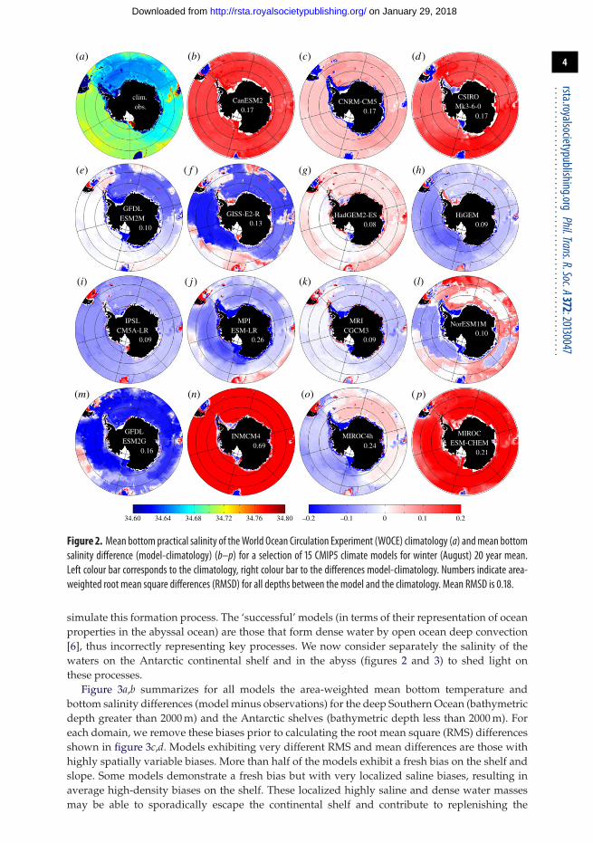
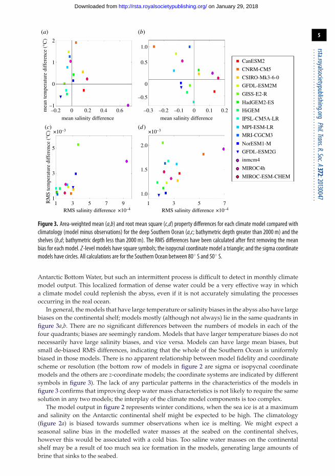
5
rstaroyalsocietypublishingorgPhilTransRSocA37220130047
0
11
10
15
20
3
5
1 3 5 73 5RMS salinity difference times10ndash4 RMS salinity difference times10ndash4
times10ndash3 times10ndash3
RM
S te
mpe
ratu
re d
iffe
renc
e (deg
C)
7 9
ndash02ndash1
0
1
2
02
mean salinity difference
mea
n te
mpe
ratu
re d
iffe
renc
e (deg
C)
04 06 ndash02
(a)
(c) (d )
(b)
ndash03
ndash05
0
05
10
ndash01
mean salinity difference
0 01 02
CanESM2
CNRM-CM5
GFDL-ESM2M
GISS-E2-R
HiGEM
IPSL-CM5A-LR
MPI-ESM-LR
MRI-CGCM3
NorESM1-M
GFDL-ESM2G
MIROC4h
MIROC-ESM-CHEM
inmcm4
HadGEM2-ES
CSIRO-Mk3-6-0
Figure 3 Area-weighted mean (ab) and root mean square (cd) property differences for each climate model compared withclimatology (model minus observations) for the deep Southern Ocean (ac bathymetric depth greater than 2000 m) and theshelves (bd bathymetric depth less than 2000 m) The RMS differences have been calculated after first removing the meanbias for each model Z-level models have square symbols the isopycnal coordinate model a triangle and the sigma coordinatemodels have circles All calculations are for the Southern Ocean between 80 S and 50 S
Antarctic Bottom Water but such an intermittent process is difficult to detect in monthly climatemodel output This localized formation of dense water could be a very effective way in whicha climate model could replenish the abyss even if it is not accurately simulating the processesoccurring in the real ocean
In general the models that have large temperature or salinity biases in the abyss also have largebiases on the continental shelf models mostly (although not always) lie in the same quadrants infigure 3ab There are no significant differences between the numbers of models in each of thefour quadrants biases are seemingly random Models that have larger temperature biases do notnecessarily have large salinity biases and vice versa Models can have large mean biases butsmall de-biased RMS differences indicating that the whole of the Southern Ocean is uniformlybiased in those models There is no apparent relationship between model fidelity and coordinatescheme or resolution (the bottom row of models in figure 2 are sigma or isopycnal coordinatemodels and the others are z-coordinate models the coordinate systems are indicated by differentsymbols in figure 3) The lack of any particular patterns in the characteristics of the models infigure 3 confirms that improving deep water mass characteristics is not likely to require the samesolution in any two models the interplay of the climate model components is too complex
The model output in figure 2 represents winter conditions when the sea ice is at a maximumand salinity on the Antarctic continental shelf might be expected to be high The climatology(figure 2a) is biased towards summer observations when ice is melting We might expect aseasonal saline bias in the modelled water masses at the seabed on the continental shelveshowever this would be associated with a cold bias Too saline water masses on the continentalshelf may be a result of too much sea ice formation in the models generating large amounts ofbrine that sinks to the seabed
on January 29 2018httprstaroyalsocietypublishingorgDownloaded from
6
rstaroyalsocietypublishingorgPhilTransRSocA37220130047
The properties of the water masses on the Antarctic continental shelf are poorly simulatedbut there is no consistent behaviour in the models studied in the formation of either dense shelfwater or abyssal water Some simulations are too fresh and others too saline and the biases on theshelf are not always the same in the deep Southern Ocean Some models probably produce densewater through unrealistic processes Does it matter that climate models are unable to representthese water masses It does especially if we need to accurately predict likely future melt ratesand stability of Antarctic ice shelves and ice sheets because the relatively warm ocean providesthe heat source for ice shelf basal melt If the climate models form too much thick sea ice that isnot advected away then this prevents heat from leaving the ocean [7] The formation of AntarcticBottom Water is a crucial part of the coupled climate system yet the climate models are unable toboth create and export water of correct characteristics
Coastal and open ocean polynyas are one of the processes that need to be better representedin climate models Although they have a relatively small geographical extent compared with sea-ice-covered regions polynyas are the sites of the most rapid and extensive changes in water massproperties through loss of heat to the atmosphere and brine rejection through sea ice formationThe next-generation climate models are evaluating ice shelf cavities [8] which may improve theshelf water properties However the fundamental problem of continental shelf edge flows can beresolved only with high horizontal and vertical resolution Even global model resolutions of 112are insufficient to be eddy permitting at high latitudes so alternative techniques may be requiredSuch methods include two-way embedded high-resolution models [9] or targeted irregular meshmodels [10]
3 Seaglider observations of Antarctic processes on the shelf and slopeThe complexity and small spatial scale of the processes on the Antarctic continental shelfand slope are not only a challenge for numerical models but they also pose a challenge forobservational oceanography and in the design of the Southern Ocean Observing System (SOOS)Regional and idealized models have suggested that the space and time scales of variability onthe Antarctic margin may be as small as O(1 km) and a couple of days [51112] These scalesare not amenable to study by ship or moorings One emerging technology is the ocean glider anautonomous underwater vehicle (AUV) able to profile the ocean for months at a time [13] Withouta propeller gliders are more energy efficient than other AUVs and data can be transmitted backto the user each time the glider surfaces (typically every 4 h for dives to 1000 m depth with divesseparated horizontally by a few kilometres) This is a great advantage in a region that is bothinaccessible for ships and covered with sea ice that can advance or break up unpredictably withindays the loss of a glider does not mean the loss of the entire dataset
Gliders can carry a range of sensors to equip them for the interdisciplinary challenges ofthe twenty-first century The standard sensors presently include temperature salinity dissolvedoxygen chlorophyll fluorescence and optical backscatter Recently developed sensors includephotosynthetically active radiation acoustic backscatter for zooplanktonmicronekton p(CO2)and pH Considerable effort is being expended worldwide to design and develop smalllightweight sensors that do not have a large energy requirement particularly for biogeochemistryand ecology In addition gliders are being deployed in ever more challenging environments suchas beneath seasonal ice cover using acoustic navigation [14]
Recently gliders have begun to be used in polar regions we discuss one such deploymentto highlight the insights that may be gained particularly at the Antarctic shelf break In January2012 three Seagliders were deployed to the east of the tip of the Antarctic Peninsula (figure 1)as part of the Gliders Excellent New Tools for Observing the Ocean (GENTOO) project The goalwas to survey the continental shelf and slope of the Weddell Sea to assess the spatial and temporalvariability of the water masses and the Slope Front Extensive sea ice in early 2012 meant that themajority of the Seaglider sections crossed the slope in the Powell Basin and progressed graduallynorthward for recovery in March
on January 29 2018httprstaroyalsocietypublishingorgDownloaded from
7
rstaroyalsocietypublishingorgPhilTransRSocA37220130047
0
0
200
(a) (b)
400
600
800
10005 10 15 20 25
distance (km)
pres
sure
(db
ar)
Seaglider ship
30 35 40 45 50 0 5 10 15 20 25distance (km)
cons
tem
pera
ture
(degC
)
30 35 40 45 50ndash2
ndash1
0
1
Figure 4 Comparison of near-simultaneous glider (a) and ship-based (b) conservative temperature sections across theAntarctic continental slope into the Weddell Sea Locations of surface measurements are indicated by the black diamonds onthe upper axis Bathymetry is shown in grey Potential density contours are shown every 01 kg mminus3 as black lines
Comparing the southernmost Seaglider section with a relatively closely-spaced ship-basedconductivityndashtemperaturendashdepth (CTD) section (figure 4) occupied at the same time theadditional small-scale structure seen by the glider is apparent A CTD station spacing of 10 kmwhich would typically resolve the submesoscale structure in mid-latitudes is problematic atthis latitude There is a suggestion of some cold water in the core of the Slope Front (40 kmalong the section at approx 400 m) but this is inadequately resolved The glider provides 10times the number of profiles and this subsurface cold water is identified on many dives bytwo independent gliders This cold water is immediately adjacent to the core of the Warm DeepWater (a warm more saline Weddell Sea water mass originating from Circumpolar Deep Watercirculating in the Weddell Sea) marking the offshore limit of the front It is isolated from the coldwater above in the Winter Water layer and the water column is statically stable It is possiblethat it represents the remnant of a diapycnal mixing process that has brought the Winter Waterdownward by 200 m However the most likely origin is from cold shelf waters that have enteredthe Antarctic Slope Current further south in the Weddell Sea and been advected northwardsMuch of the small-scale structure seen in the glider data is associated with internal wavesparticularly on the sharp boundary at the base of the temperature-minimum layer (Winter Water)However the small subsurface lenses of warmer water at 20ndash35 km indicate that Warm DeepWater has crossed the Slope Front onto the continental shelf Such bidirectional cross-frontal andcross-slope exchange processes are likely to be important for the exchange of nutrients larvae andcarbon between the open ocean and continental shelf
Figure 5 shows an example Seaglider section across the continental slope of the PowellBasin downstream of the section shown in figure 4 At the seabed we see the cold water core(figure 5a) that has spilled off the continental shelf further south in the Weddell Sea and is nowbeing exported from the Powell Basin to form what will eventually be termed Antarctic BottomWater It is relatively rich in dissolved oxygen (figure 5d) compared with the Warm Deep Waterabove it indicating that it was recently ventilated Optical backscatter (figure 5e) is also slightlyelevated in this cold layer suggesting that the flow here is bottom-enhanced sufficiently fastto suspend sediments in a thick nepheloid layer The V-shaped isotherms and isohalines thatindicate the location of the Antarctic Slope Front are apparent at an along-track distance of 102 kmChlorophyll a concentrations show a consistent pattern of more chlorophyll a near the Slope Frontand on the continental shelf than in the open Weddell Sea This suggests greater phytoplanktongrowth on the shelf perhaps owing to enhanced surface stratification or to sedimentary sourcesof iron
4 Antarctic shelf influence on iron concentrationsThe Southern Ocean plays a significant role in the drawdown of anthropogenic CO2 yet thisremains poorly constrained [15] It is now known as a region where the limiting trace element forprimary productivity is iron [16] One source of iron is from dust from continental weathering
on January 29 2018httprstaroyalsocietypublishingorgDownloaded from
8
rstaroyalsocietypublishingorgPhilTransRSocA37220130047
0
0 5
(a)
10distance (km)
pres
sure
(db
ar)
15 20 0 5 10 15 20
abs
sal
inity
(g
kgndash1
)
200
400
600
800
1000
0(b)
cons
tem
pera
ture
(degC
)
200
400
600
800
1000ndash2 338
340
342
344
346
348
ndash1
0
1
0
0 5
(e) ( f )
10distance (km)
pres
sure
(db
ar)
15 2056deg W
64deg S
30
30
30
63deg S
62deg S
54deg W 52deg W 50deg W 48deg W
200
400
600
800
1000
back
scat
ter
60
70
80
90
0
0 5
(c)
10distance (km)
pres
sure
(db
ar)
15 20 0 5 10 15 20
oxyg
en (
mmol
kgndash1
)
200
400
600
800
1000
0(d )
chlo
roph
yll a
(m
gm
ndash3)
200
400
600
800
100002 150
200
250
300
350
04
06
08
Figure 5 An example Seaglider section from the continental shelf (distance 0 km) into Powell Basin (distance 20 km) of(a) conservative temperature (C) (b) absolute salinity (g kgminus1) (c) chlorophyll a concentration (mg mminus3) calculated usinga factory calibration and not calibrated against in situ phytoplankton assemblages (d) dissolved oxygen (micromol kgminus1) and(e) optical backscatter signal strength (uncalibrated counts) The locations of glider surfacings are indicated as black diamondson the upper axes The seabed is shown in grey deduced from General Bathymetric Chart of the Oceans (GEBCO) atlas data(f ) The location of the section is indicated in red togetherwith bathymetric contours every 500 m The 1000 and 3000 mcontoursare shown in bold
deposited in the ocean after atmospheric transport or glacial melt inputs are generally small inthe Southern Ocean owing to its distance from non-ice-covered continental land masses Icebergsalso transport iron from the continental margin and have been shown to enhance productivity[17] However the most significant iron source to the Southern Ocean is likely to be the iron-rich sediment on the continental shelves and shallow plateaus surrounding the continent and thesub-Antarctic islands Numerical ecosystem modelling studies of the influence of iron [18] havehad some success in capturing the spatial distribution in productivity A study of the sensitivityof the productivity to these iron sources [19] uses a much simpler iron-cycling model embeddedin an eddy-permitting ocean circulation model It has three iron reservoirs dissolved iron ironwithin the living plankton and sinking or particulate iron The modelrsquos predicted dissolved irondistribution (figure 6) demonstrates the importance of the Antarctic continental shelves as aniron source Dissolved iron concentrations are highest in the mixed layer around AntarcticaComparison with figure 1 confirms the large mixed layer iron concentrations in the continentalshelf regions inshore of the Antarctic Slope Front but also reveals that the iron is being exportedoff the shelf The model output suggests that sediment provides some 90 of the usable ironin the Southern Ocean and icebergs the remaining 10 Additional localized sources includedust deposition (eg downwind of Patagonia) Sediment fluxes on the Antarctic continental shelfand slope must be able to cross the barrier of the Antarctic Slope Front in order to fertilize theopen ocean emphasizing the importance of the cross-slope processes in transporting nutrients aswell as biota Icebergs provide one route in which such nutrients may cross such a boundary
on January 29 2018httprstaroyalsocietypublishingorgDownloaded from
9
rstaroyalsocietypublishingorgPhilTransRSocA37220130047
0 02 04
180deg W
80deg S
70deg S
60deg S
50deg S
0deg
120deg
E120degW
60deg E60
degW
FeD (nmol Fe lndash1)
06 08 10
Figure 6 Annual mean distribution of dissolved iron (nmol lminus1) in the ocean mixed layer of an iron-cycling model driven bythe likely sources of iron (dust icebergs and sedimentary) [19]
Antarctica
ice shelf
Ekmantransport
deep waterformation
eddies grow out of barotropicand baroclinic instabilities ofthe Antarctic Slope Current
eddies
wind
along
-isop
ycna
l
mixing
Figure 7 Schematic to summarize the principal processes acting at the Antarctic continental shelf break that are involved inthe exchange of water masses heat freshwater nutrients andor biota
The processes of eddy overturning and frontal instability [5] as observed by the glider datadiscussed in sect3 may also play a role Icebergs and shelf water both contribute sources of ironto the exceptional productivity seen in the Scotia Sea within an otherwise unproductive iron-limited Southern Ocean The high-resolution (112) model in which iron cycling is embedded isable to simulate such processes However it is important to note that such a high resolution is notyet possible in the Earth system models and therefore the role of the Antarctic continental shelfin global scale carbon cycling may remain underestimated
5 ConclusionWe have shown examples to illustrate the importance of the Antarctic continental slope andshelf for climate and for biogeochemistry highlighting that a relatively small area can have adisproportionately large influence on global ocean properties Figure 7 summarizes schematically
on January 29 2018httprstaroyalsocietypublishingorgDownloaded from
10
rstaroyalsocietypublishingorgPhilTransRSocA37220130047
the processes at the Antarctic shelf break that are important for cross-slope exchange ofheat freshwater nutrients such as iron or larvae and other biota It is clear that we areonly just beginning to have the tools available to understand these polar processes let aloneto parameterize them in a suitable way for their inclusion in global Earth system modelsOcean gliders offer great potential for observing Antarctic processes they can undertake multi-disciplinary missions for some months without a ship being in attendance The Seaglider resultsshown here identified ocean features that could not feasibly have been studied by any othermeans furthermore such eddy processes are likely to be common all around the Antarcticmargin It is likely therefore that gliders can have an important role in the future SOOS forcontinental shelves and slopes along with other new technologies such as miniature sensorscarried by marine mammals Better understanding of the processes must be obtained concurrentlywith the development of new modelling techniques to improve the representation of SouthernOcean water masses in climate models
Acknowledgements The paper is dedicated in memory of Eberhard Fahrbach world-leading polaroceanographer whose ideas and enthusiasm inspired us and othersFunding statement This research was carried out on the High Performance Computing Cluster supported bythe Research and Specialist Computing Support service at UEA We thank Caltech iRobot and UEA forsupporting the Seaglider campaign NERC research funding supported the iron modelling (NEC50633X1)Seaglider deployments (NEH01439X1 and NEH0147561) and CMIP5 model analysis (NEI0182391)JKR is supported by the Joint DECCDefra Met Office Hadley Centre Climate Programme (GA01101)We acknowledge the WCRPrsquos Working Group on Coupled Modelling responsible for CMIP and thank theCMIP5 climate modelling groups for releasing their model output CMIP5 datasets are available throughtheir portal the oceanographic observed datasets are available from BODC For the iron-cycling model codecontact Martin Wadley (mwadleyueaacuk)
References1 Schmidtko S Johnson GC Lyman JM 2013 MIMOC a global monthly isopycnal upper-ocean
climatology with mixed layers J Geophys Res Oceans 118 1658ndash1672 (doi101002jgrc20122)2 Rintoul SR Hughes C Olbers D 2001 The Antarctic circumpolar current system In Ocean
circulation and climate (eds JCG Siedler J Gould) pp 271ndash302 San Diego CA Academic Press3 Pritchard HD Ligtenberg SRM Fricker HA Vaughan DG van den Broeke MR Padman
L 2012 Antarctic ice-sheet loss driven by basal melting of ice shelves Nature 484 502ndash505(doi101038nature10968)
4 Heywood KJ Muench R Williams G 2012 An overview of the Synoptic Antarctic ShelfndashSlope Interactions (SASSI) project for the international polar year Ocean Sci 8 1111ndash1116(doi105194os-8-1111-2012)
5 Stewart AL Thompson AF 2013 Connecting Antarctic cross-slope exchange with southernocean overturning J Phys Oceanogr 43 1453ndash1471 (doi101175JPO-D-12-02051)
6 Heuzeacute C Heywood KJ Stevens DP Ridley J 2013 Southern ocean bottom water characteristicsin CMIP5 models Geophys Res Lett 40 1409ndash1414 (doi101002grl50287)
7 Richardson G Wadley MR Heywood KJ Stevens DP Banks HT 2005 Short-term climateresponse to a freshwater pulse in the southern ocean Geophys Res Lett 32 L03702(doi1010292004GL021586)
8 Kusahara K Hasumi H 2013 Modeling Antarctic ice shelf responses to future climate changesand impacts on the ocean J Geophys Res 118 2454ndash2475 (doi101002jgrc20166)
9 Debreu L Marchesiello P Penven P Cambon G 2012 Two-way nesting in splitndashexplicitocean models algorithms implementation and validation Ocean Model 49ndash50 1ndash21(doi101016jocemod201203003)
10 Scholz P Lohmann G Wang Q Danilov S 2013 Evaluation of a finite-element sea-ice oceanmodel (FESOM) set-up to study the interannual to decadal variability in the deep-waterformation rates Ocean Dyn 63 347ndash370 (doi101007s10236-012-0590-0)
11 Dinniman MS Klinck JM Smith Jr WO 2011 A model study of Circumpolar Deep Water onthe West Antarctic Peninsula and Ross Sea continental shelves Deep-Sea Res II 58 1508ndash1523(doi101016jdsr2201011013)
on January 29 2018httprstaroyalsocietypublishingorgDownloaded from
11
rstaroyalsocietypublishingorgPhilTransRSocA37220130047
12 Wang Q Danilov S Schroumlter J 2008 Bottom water formation in the southern Weddell Sea andthe influence of submarine ridges idealized numerical simulations Ocean Model 28 50ndash59(doi101016jocemod200808003)
13 Eriksen CC Osse TJ Light RD Wen T Lehman TW Sabin PL Ballard JW Chiodi AM 2001Seaglider a long-range autonomous underwater vehicle for oceanographic research IEEE JOcean Eng 26 424ndash436 (doi10110948972073)
14 Lee C et al 2010 Autonomous platforms in the Arctic observing network In Proc OceanObs09Sustained Ocean Observations and Information for Society Conf (vol 2) Venice Italy 21ndash25September 2009 (eds J Hall DE Harrison D Stammer) ESA Publication WPP-306 NoordwijkThe Netherlands European Space Agency
15 Sabine CL et al 2004 The oceanic sink for anthropogenic CO2 Science 305 367ndash371 (doi101126science1097403)
16 Boyd PW 2002 The role of iron in the biogeochemistry of the Southern Ocean andequatorial Pacific a comparison of in situ iron enrichments Deep-Sea Res II 49 1803ndash1821(doi101016S0967-0645(02)00013-9)
17 Geibert W et al 2010 High productivity in an ice melting hot spot at the eastern boundary ofthe Weddell Gyre Glob Biogeochem Cycles 24 GB3007 (doi1010292009gb003657)
18 Lancelot C de Montety A Goosse H Becquevort S Schoemann V Pasquer B VancoppenolleM 2009 Spatial distribution of the iron supply to phytoplankton in the Southern Ocean amodel study Biogeoscience 6 2861ndash2878 (doi105194bg-6-2861-2009)
19 Wadley MR Jickells TD Heywood KJ 2014 The role of iron sources and transport for SouthernOcean productivity Deep-Sea Res I 87 82ndash94 (doi101016jdsr201402003)
on January 29 2018httprstaroyalsocietypublishingorgDownloaded from
- Introduction
- Representation of Antarctic shelf and slope processes in climate models
- Seaglider observations of Antarctic processes on the shelf and slope
- Antarctic shelf influence on iron concentrations
- Conclusion
- References
-
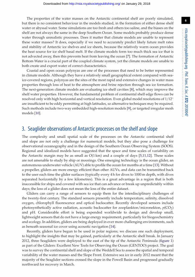
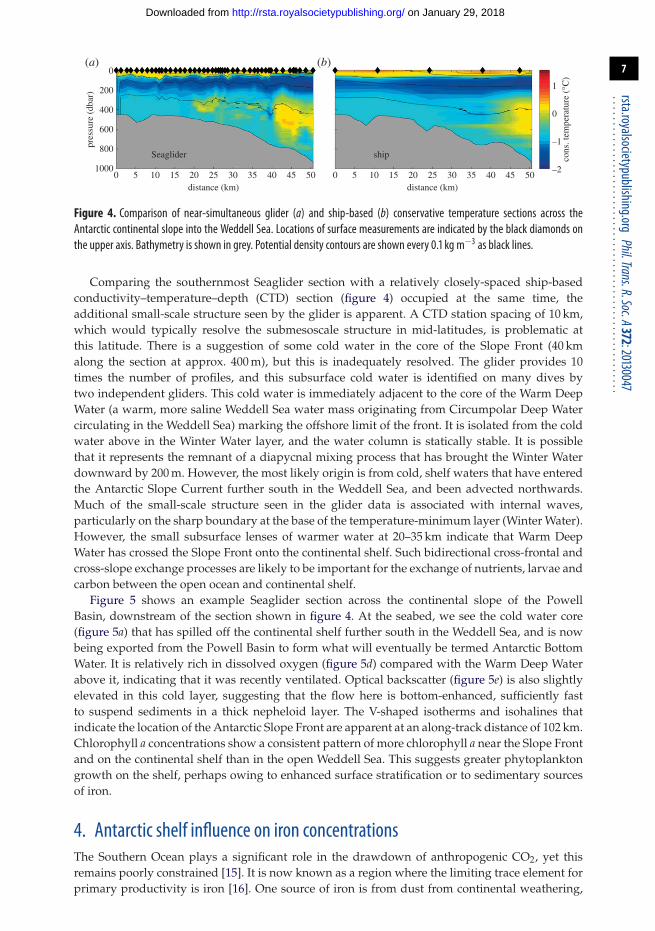
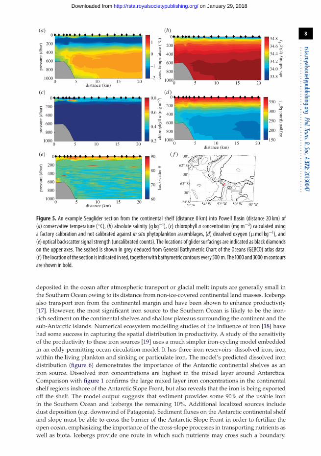
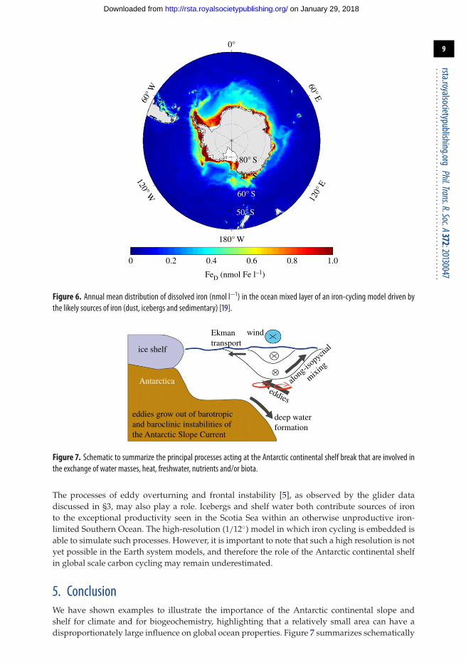
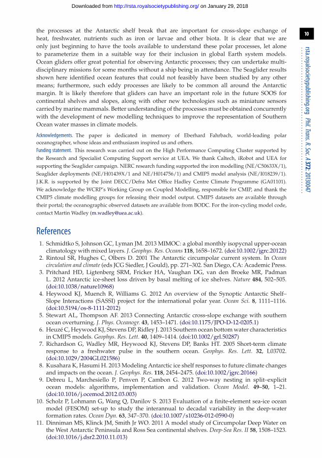


