acceleration and overturning of the antarctic slope

Acceleration and Overturning of the Antarctic Slope Current by Winds,Eddies, and Tides

ANDREW L. STEWART

Department of Atmospheric and Oceanic Sciences, University of California, Los Angeles, Los Angeles, California

ANDREAS KLOCKER

Antarctic Climate and Ecosystems Cooperative Research Centre, University of Tasmania, Hobart, Australia

DIMITRIS MENEMENLIS

Science Division, Jet Propulsion Laboratory, California Institute of Technology, Pasadena, California

(Manuscript received 26 October 2018, in final form 27 May 2019)

ABSTRACT

All exchanges between the open ocean and the Antarctic continental shelf must cross the Antarctic Slope

Current (ASC). Previous studies indicate that these exchanges are strongly influenced by mesoscale and tidal

variability, yet the mechanisms responsible for setting the ASC’s transport and structure have received rel-

atively little attention. In this study the roles of winds, eddies, and tides in accelerating the ASC are in-

vestigated using a global ocean–sea ice simulation with very high resolution (1/488 grid spacing). It is found

that the circulation along the continental slope is accelerated both by surface stresses, ultimately sourced from

the easterly winds, and by mesoscale eddy vorticity fluxes. At the continental shelf break, the ASC exhibits a

narrow (;30–50 km), swift (.0.2m s21) jet, consistent with in situ observations. In this jet the surface stress is

substantially reduced, andmay even vanish or be directed eastward, because the ocean surface speedmatches

or exceeds that of the sea ice. The shelfbreak jet is shown to be accelerated by tidal momentum advection,

consistent with the phenomenon of tidal rectification. Consequently, the shoreward Ekman transport van-

ishes and thus the mean overturning circulation that steepens the Antarctic Slope Front (ASF) is primarily

due to tidal acceleration. These findings imply that the circulation and mean overturning of the ASC are not

only determined by near-Antarctic winds, but also depend crucially on sea ice cover, regionally-dependent

mesoscale eddy activity over the continental slope, and the amplitude of tidal flows across the continental

shelf break.

1. Introduction

TheAntarctic Slope Current (ASC) is an approximately

circumpolar, westward flow that tracks the continental

shelf break and slope (see Fig. 1 and Thompson and

Heywood 2008; Meijers et al. 2010; Chavanne et al. 2010;

Armitage et al. 2018). A portion of the ASC is associated

with the Antarctic Slope Front (ASF), a subsurface front

that separates increasingly warm waters at middepth

(;300m) offshore (Schmidtko et al. 2014) from the typi-

cally cold waters of the continental shelf (Jacobs 1991;

Whitworth et al. 1998). The ASC and ASF therefore me-

diate exchanges of waters across the Antarctic continental

slope and exert an outsized influence on local and global

ocean circulation and climate (Rintoul 2018; Thompson

et al. 2018). For example, transfer of heat from the open

ocean onto the continental shelf must cross the ASF

(Heywood et al. 2016; Goddard et al. 2017; Palóczy et al.

2018) and directly contributes to the melt of Antarctica’s

floating ice shelves (Pritchard et al. 2012; Jenkins et al.

2016; Zhao et al. 2019). The production of dense shelf

waters (DSW) supply the global volume of Antarctic

Bottom Water (Gordon 2001; Orsi et al. 2001), which in

turn ventilates the abyssal ocean (Sarmiento et al. 1988;

Hotinski et al. 2001) and contributes to the baroclinicity

and structure of the Antarctic Circumpolar Current

(ACC) (Morrison and Hogg 2013; Stewart and Hogg

2017).

Despite the ASC’s significance in the global ocean

circulation, relatively little is understood about itsCorresponding author: Andrew L. Stewart, [email protected]

AUGUST 2019 S TEWART ET AL . 2043

DOI: 10.1175/JPO-D-18-0221.1

� 2019 American Meteorological Society. For information regarding reuse of this content and general copyright information, consult the AMS CopyrightPolicy (www.ametsoc.org/PUBSReuseLicenses).

mailto:[email protected]

http://www.ametsoc.org/PUBSReuseLicenses



circulation and dynamics compared, for example, to the

ACC farther north (Rintoul 2018). The conception of

the flow along theAntarctic shelf break as a wind-driven

current was introduced by Gill (1973) and persists in

modern descriptions of the ASC (Heywood et al. 2014).

Process-oriented models of the ASF indicate that the

wind-driven shoreward Ekman transport plays a central

role in setting the slope of the pycnocline in theASF and

thus the overturning circulation across continental shelf

and slope (Nøst et al. 2011; Stewart andThompson 2015a;

Hattermann 2018). This suggests that the near-Antarctic

circulation, shoreward heat transport, and export of

DSW to the global abyss should all be sensitive to changes

in the near-Antarctic winds (Stewart and Thompson 2012;

Spence et al. 2014, 2017; Goddard et al. 2017).

One way in which recent conceptions of the ASF/

ASC have advanced upon that of Gill (1973) is in

their identification of the role of mesoscale variabil-

ity, which we refer to as ‘‘eddies’’ throughout this ar-

ticle, in mediating cross-slope exchanges (Klinck and

Dinniman 2010; Thompson et al. 2014). In parallel with

the well-established paradigm for the ACC (Marshall

and Radko 2003; Abernathey et al. 2011), eddies might

be expected to counteract wind-induced steepening of

isopycnals and thereby contribute to setting the bar-

oclinicity of the ASF (Nøst et al. 2011; Stewart and

Thompson 2013). Previous studies indicate that eddies

efficiently transfer heat toward the coast via troughs in

the continental shelf, particularly where circumpolar

deep water (CDW) floods the shelf (St-Laurent et al.

2013; Couto et al. 2017) and where DSW is exported

across the continental slope (Thompson et al. 2014;

Stewart and Thompson 2015b). Stewart and Thompson

(2016) examined the role of eddies in the momentum

balance of the ASC, using idealized simulations, and

found that they accelerated a series of jets along the

continental slope, which in turn drifted offshore.

In addition to eddies, the ASC also experiences

strong tidal flows, with average tidal velocities reach-

ing O (1)m s21 around localized stretches of the shelf

break (e.g., Foldvik et al. 1990; Robertson 2001). Tides

can contribute substantially to exchanges of CDW and

FIG. 1. Speed of the time-mean depth-averaged flow in the LLC_4320 simulation,

highlighting the circumpolar structure of the Antarctic Slope Current’s shelf break jet. The

overlays and labels indicate our division of the Antarctic margins into regions, following

Stewart et al. (2018).

2044 JOURNAL OF PHYS ICAL OCEANOGRAPHY VOLUME 49

DSW across the continental shelf and slope, particu-

larly where the slope is relatively steep (Padman et al.

2009; Wang et al. 2013; Castagno et al. 2017). Tidal

rectification can also directly contribute to the accel-

eration of along-slope mean flows, which are neces-

sary to conserve momentum against the along-slope tidal

‘‘Stokes’ drift’’ (Garreau and Maze 1992; Chen and

Beardsley 1995), for example, around Georges Bank

(Loder 1980) and the Yellow Sea (Lee and Beardsley

1999). Flexas et al. (2015) found that regional simulations

integrated with tidal forcing alone could produce an ASF

in the Weddell–Scotia confluence, suggesting that tides

play a key role on driving the ASC there. However, it

remains unclear whether this tidal acceleration of the

ASC is ubiquitous around theAntarctic shelf or limited to

specific ‘‘hot spots’’ such as the Weddell Sea.

In this article we use a global simulation with very

high resolution (see Stewart et al. 2018) to examine

the relative roles of wind forcing and transient flows

(eddies and tides) in driving the ASC. In section 2

we discuss the model and our approach to analyzing it:

we first review the model configuration (section 2a),

compare the structure of the simulated ASC against

high-resolution hydrography and current measure-

ments (section 2b), and provide diagnostics of the

ASC’s mean circulation and forcing (section 2c). We

then describe our temporal decomposition of the

model variables into approximate mean, eddy, and

tidal components (section 2d), and discuss our trans-

formation to coordinates that approximately follow

the mean flow of the ASC (section 2e). In section 3 we

present our main results: we first quantify the rela-

tive importance of different ASC circulation drivers

via the integrated vorticity budget (section 3a) and

energy budget (section 3b) in the combined Amery/

East Antarctica sector (see Fig. 1), which we use as a

reference case because the ASC is approximately

zonal there. We then examine the localization of the

ASC forcing as a function of along-coast distance

(section 3c) and depth (section 3d), and quantify

variations in this forcing between different sectors of

the continent (section 3e). Finally, we discuss our re-

sults and draw conclusions in section 4.

2. The ASC in the LLC_4320 simulation

This section describes the tools and methods required

to distinguish different drivers of the ASC circulation in

section 3. We first provide an overview of the simula-

tion that serves as the basis of our analysis, referred to as

the latitude–longitude–cap 4320 (LLC_4320) simulation

(Rocha et al. 2016), and evaluate the simulated ASC

against observations. We additionally present diagnostics

of the mean zonal flow and surface/bottom forcing of the

ASC. These diagnostics motivate a decomposition of the

model variables into mean, eddy, and tidal components

and a transformation into a coordinate system that fol-

lows isobaths (see Stewart et al. 2018).

a. Model configuration

We draw our results from a global ocean–sea ice

simulation (the LLC_4320) run at very high horizontal

resolution (Rocha et al. 2016), having a grid spacing of

1/488, or ;1 km over the Antarctic continental shelf

and slope. In the vertical, the model is discretized into

90 levels, with spacings ranging from 1m at the surface

to 480m at a depth of 7000m. Previous studies have

found that this approximate model resolution is re-

quired to resolve eddy- and tidal-driven heat and vol-

ume exchanges across the continental slope (Padman

et al. 2009; St-Laurent et al. 2013; Wang et al. 2013;

Stewart and Thompson 2015b; Graham et al. 2016).

At this time, no other model simulation that includes

tidal forcing and spans the entire Antarctic margins

has achieved comparable resolution. The LLC_4320

therefore offers a unique, albeit preliminary, insight

into the role of high-frequency variability over the

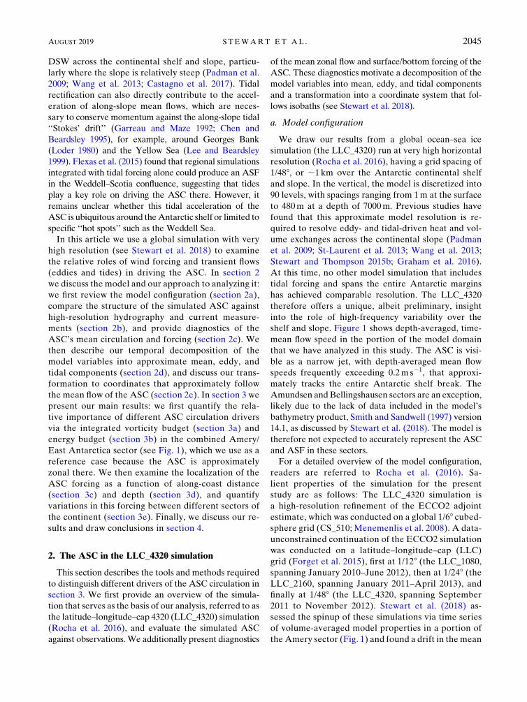
shelf and slope. Figure 1 shows depth-averaged, time-

mean flow speed in the portion of the model domain

that we have analyzed in this study. The ASC is visi-

ble as a narrow jet, with depth-averaged mean flow

speeds frequently exceeding 0.2m s21, that approxi-

mately tracks the entire Antarctic shelf break. The

Amundsen and Bellingshausen sectors are an exception,

likely due to the lack of data included in the model’s

bathymetry product, Smith and Sandwell (1997) version

14.1, as discussed by Stewart et al. (2018). The model is

therefore not expected to accurately represent the ASC

and ASF in these sectors.

For a detailed overview of the model configuration,

readers are referred to Rocha et al. (2016). Sa-

lient properties of the simulation for the present

study are as follows: The LLC_4320 simulation is

a high-resolution refinement of the ECCO2 adjoint

estimate, which was conducted on a global 1/68 cubed-sphere grid (CS_510; Menemenlis et al. 2008). A data-

unconstrained continuation of the ECCO2 simulation

was conducted on a latitude–longitude–cap (LLC)

grid (Forget et al. 2015), first at 1/128 (the LLC_1080,

spanning January 2010–June 2012), then at 1/248 (theLLC_2160, spanning January 2011–April 2013), and

finally at 1/488 (the LLC_4320, spanning September

2011 to November 2012). Stewart et al. (2018) as-

sessed the spinup of these simulations via time series

of volume-averaged model properties in a portion of

the Amery sector (Fig. 1) and found a drift in the mean


potential temperature of 0.18–0.158C over two years of

LLC_2160 output. In contrast, the volume-averaged

kinetic energy did not exhibit any drift, and in section 3

we similarly find that the tendency in the along-slope

circulation is orders of magnitude smaller than the vari-

ous terms contributing to its acceleration.

In all cases themodel was forced by atmospheric fields

derived from the 0.148 ECMWF operational analysis

(ECMWF 2011) and a tidal potential that includes the

16 frequencies corresponding to the largest global am-

plitudes (see Rocha et al. 2016). Continental runoff,

including ice shelf melt and calving, is prescribed as a

constant 1743Gt yr21 (Fekete et al. 2002), distributed

in a 200-kmband around the coastline ofAntarctica, and

applied to the uppermost geopotential grid level at each

horizontal location. Apart from the prescribed time-

mean surface runoff, the above simulations do not in-

clude an explicit representation of ice shelf cavities or of

bottom boundary layer processes, which likely inhibit

the model’s ability to realistically represent DSW for-

mation and export. The results in the main text of this

article are diagnosed exclusively from the LLC_4320

simulation. However, Stewart et al. (2018) found

that the mean/eddy/tidal cross-slope heat fluxes ex-

hibited only small quantitative differences between

the LLC_4320 and LLC_2160 simulations, despite the

larger ;2 km grid spacing of the LLC_2160 simulation.

Therefore, due to the very high computational cost of

performing analysis on the LLC_4320 simulation, we

perform supplementary tests (see appendixes B and C)

using output from the LLC_2160 simulation.

b. Evaluation of simulated ASF structure

Before proceeding to our analysis of the LLC_4320

simulation, we first address the model’s representation of

the ASC and ASF. Our ability to perform quantitative

evaluation of the model state is limited by the paucity of

observations; we require in situ measurements of both

hydrography and velocity that are able to resolve the

narrow (tens of kilometers wide) core of the ASC. Here

we focus on measurements from the Amery sector (see

Fig. 1) because high-resolution velocity and hydrographic

measurements are available. Additionally, we use the

combined Amery/East Antarctica sector as a reference

case throughout section 3 because the ASC, and thus its

momentum forcing, are approximately zonal. In appendix

A we present an additional model-observation compari-

son using measurements from the western Weddell Sea.

Figure 2 shows a comparison of the LLC_4320 model

state with measurements made during the BROKEWest

survey along 608E (Meijers et al. 2010). Here we have

averaged the model fields over the ;1-year duration of

FIG. 2. Evaluation of the (b),(d) modeled annual-mean Antarctic Slope Front/Current against (a),(c) observations

made between 8 and 11 Feb 2006 during the BROKE West Survey along 608E (Meijers et al. 2010). (top) Potential

temperature (colors) and neutral density (black contours) calculated following Jackett and McDougall (1997).

Labels indicate neutral densities on each isopycnal (kgm23). (bottom) Zonal velocity contoured every 0.01m s21

(colors) and 0.04m s21 (black contours). In (a) and (c), the dashed black lines indicate locations at which CTD cast

and lowered ADCP measurements were taken.


the LLC_4320 simulation because the seasonal mean

model state exhibits only relatively small quantitative

differences from Figs. 2b and 2d, and for consistency with

the annually averaged model diagnostics discussed in

section 3. The modeled and observed hydrographies in

Figs. 2a and 2b are qualitatively similar despite inevitable

sampling biases associated with temporal variability, and

despite the model output having been annually averaged.

Note that we have not attempted to evaluate the temporal

variability in, for example, the transport of the ASC

(Peña-Molino et al. 2016), because the LLC_4320 simu-

lation contains only a single seasonal cycle. In particular, a

strong front in the temperature field, characteristic of

theASF (Jacobs 1991;Whitworth et al. 1998), is present at

the shelf break in both the model and the observations.

A notable deficiency in the model is the absence of cold,

dense water at the sea floor, indicating a lack of DSW

production and export, likely due to the relatively short

spinup from the ECCO2 adjoint estimate combined with

the absence of ice shelf cavities. Themodel therefore likely

omits eddy generation resulting from DSW export (Lane-

Serff and Baines 1998; Stewart and Thompson 2016); this

should be regarded as a caveat to our analysis. The

differences in hydrography are more pronounced in

the westernWeddell Sea, where DSW is present across

the entire continental slope (see appendix A).

Figures 2c and 2d show that the simulated andobserved

along-slope currents are also qualitatively similar to one

another, though the quantitative differences are more

evident than they are in the hydrography. Both themodel

and observations exhibit a narrow (;30–40km wide)

westward jet at the shelf break, though the modeled jet

exhibits a somewhat larger maximum speed (0.3ms21)

than the observed jet (0.24ms21). It is unclear whether

the differences visible in Figs. 2c and 2d are the result of

model biases or whether they are largely a consequence

of spatiotemporal sampling limitations (e.g., Peña-Molino et al. 2016). In either case, we conclude that the

modeled ASF and ASC are at least representative of

those in the ocean, with the exception of DSW influences.

c. Mean circulation and forcing of the ASC

In this study our primary aim is to distinguish different

drivers of ASC circulation, so our diagnostics focus on

the model momentum budget. The LLC_4320 is based

on the Massachusetts Institute of Technology general

circulationmodel (MITgcm;Marshall et al. 1997a,b) and

solves the Boussinesq momentum equations in vector-

invariant form,

›u

›t52f z3u2 zz3 u2w

›u

›z2=f2=

�1

2u2

�

1›t(z)

›z1G

n1G

t. (1)

Here u5 (u, y) is the horizontal velocity vector, w is the

vertical velocity, f is the dynamic pressure, z5 z � =3 u

is the vertical component of relative vorticity, and f is

the Coriolis parameter. We denote the vertical stress as

t(z), defined such that positive values correspond to

downward momentum transfer. The divergence of the

lateral viscous stress tensor is denoted Gn and is pre-

scribed via a modified Leith formulation (Fox-Kemper

and Menemenlis 2008). Finally, Gt represents the tide-

producing force, which is a sum of temporally oscillatory

functions at each point in space, and so vanishes ap-

proximately under the long (;1 year) time averages

considered in this paper.

To make explicit the role of surface and bottom mo-

mentum forcing, we perform most of our analysis on the

depth integral of (1), defining

hdi[ð02h

dz d , (2)

where z52h(x, y) is the sea floor elevation. To

examine different drivers of the time-mean circu-

lation, we additionally define a time averaging

operator

d[1

T

ðt01T

t0

dt d , (3)

where t0 and T denote the start and duration of the

averaging period, respectively. This operator will be

generalized to multiple time scales in section 2d. The

depth-integrated time-mean momentum equation is

therefore

[hui]t|fflffl{zfflffl}

Tendency

52f z3 hui|fflfflfflfflfflfflffl{zfflfflfflfflfflfflffl}Coriolis

2z3 hzui2�w›u

›z

�|fflfflfflfflfflfflfflfflfflfflfflfflfflfflfflfflffl{zfflfflfflfflfflfflfflfflfflfflfflfflfflfflfflfflffl}

Advection

2h=fi|fflfflfflffl{zfflfflfflffl}Pressure gradient

2

�=

�1

2u2

��|fflfflfflfflfflfflfflfflfflfflffl{zfflfflfflfflfflfflfflfflfflfflffl}

KE gradient

1tjz50|fflfflfflffl{zfflfflfflffl}

Surface stress

2tjz52h|fflfflfflfflffl{zfflfflfflfflffl}

Bottom stress

1hGni|fflfflffl{zfflfflffl}

Viscosity

1hGti|fflfflffl{zfflfflffl}

Tidal potential

, (4)


where we define [d]t [ (djt01T 2 djt0)/T. Note that, fol-

lowing (1), the surface and bottom stresses are divided

by the reference density, and so have units of meters

squared per second squared (m2s22). The ocean surface

stress is calculated via standard quadratic bulk formulae for

the atmosphere–ocean and sea ice–ocean stresses, weighted

by the open water fraction and sea ice concentration, re-

spectively. For further details, see Losch et al. (2010).

Figure 3 illustrates the mean circulation of the ASC in

the combined Amery/East Antarctica sector (see Fig. 1).

Figure 3a shows the potential temperature at 230-m

depth, highlighting variations in the sharpness of the

ASF as it passes troughs in the continental shelf, visible in

Fig. 3a as locations where the 500-m isobath deviates

toward the coastline. These troughs also guide the depth-

integrated mean flow closer to the coast, as can be seen in

the barotropic streamfunction in Fig. 3b. Here the baro-

tropic streamfunction is defined as

C[

ðyys

hui dy0 , (5)

where ys is the southernmost latitude for which the

ocean depth h is nonzero and y0 is a variable of integration.Figure 3b also shows that most of the transport of theASC

occurs offshore of the ASF, at depths greater than 2000m,

with only a few Sverdrups (Sv; 1Sv[ 106m3 s21), of along-

slope transport at the shelf break (see Peña-Molino et al.

2016). However, the ASF consistently coincides with the

strongest westward velocities in the ASC (Fig. 3c), which

exhibits a jet with a meridional width of tens of kilometers

andmaximum speeds exceeding 0.3ms21 (see also Fig. 2).

As discussed in section 1, previous studies have typi-

cally characterized the ASC as a wind-driven circula-

tion, so we first examine the role of wind in driving the

model’s ASC. In Figs. 4a and 4b we plot the zonal stress

at the ocean surface over the same region as shown in

Fig. 3. Note that throughout this article we plot all terms

in the momentum budget in the more familiar units of

newtons per square meter (Nm22) [i.e., multiplying (4)

by r0]. The surface stress is directed westward almost

everywhere due to the easterly winds that encircle the

Antarctic margins (see, e.g., Large and Yeager 2009;

ECMWF 2011), with a zonal-mean maximum westward

stress of around 0.06Nm21 (Fig. 4b). However, there

is a band of weak or zero westward stress, and in some

places even weak eastward stress, tracking the shelf

break. The meridional width of this feature is compa-

rable to that of the shelfbreak jet shown in Fig. 3, and

much smaller than the typical scales of variability in the

local atmospheric circulation (Langlais et al. 2015).

Understanding the surface stress over the shelfbreak

jet requires consideration of the sea ice, which covers the

ASC for most of the year (e.g., Cavalieri and Parkinson

2008). Figure 3d shows that the sea ice also drifts west-

ward due to the easterly winds, with amean speed that is

typically faster than that of the sea surface, such that the

westward momentum input by the wind is transferred

down to the ocean via ice–ocean drag (Losch et al. 2010;

Meneghello et al. 2018). An exception occurs over the

shelf break, where the mean sea ice speed exhibits a

similar jet over the shelf break as the mean ocean sur-

face speed (Fig. 3c), and the ice–ocean shear approxi-

mately vanishes (Fig. 3e). In contrast, Fig. 4b shows that

the zonal stress at the sea floor is elevated at the shelf

break because the shelf break jet is largely barotropic

(see Fig. 2). Longitudinal variations of the shelfbreak

latitude obscure this elevated bottom stress in a zonal

average, however, with typical zonal-mean bottom

stresses of around 0.01Nm21. Note that the time-mean

flows and surface/bottom stresses discussed here also

obscure the seasonal variations in the forcing of the

ASC, which are discussed in appendix C.

d. Temporal decomposition

While the diagnostics presented in the preceding

section indicate that the ASC is primarily forced by

momentum transfer from the wind via the sea ice, the

approximate vanishing of the surface stress in the core of

the ASC (Fig. 4a) indicates that an alternative forcing

mechanism must be present there. Lacking other inputs

of mean momentum in (4), we anticipate that the ASC

jet core may be the result of an interaction between

mean and transient flows, as arise in a wide range of

contexts in geophysical fluid dynamics (e.g., Andrews

and McIntyre 1976; Bühler 2014).As discussed in section 1, previous studies of the

Antarctic shelf and slope emphasize both eddy and tidal

variability. We therefore pose an approximate decom-

position of themodel variables intomean, eddy and tidal

components to distinguish their relative roles in driving

the ASC, following Stewart et al. (2018). For example,

the model horizontal velocity field is written as a sum of

mean um, eddy ue, and tidal ut components,

u5um1 u

e1 u

t. (6)

We define the operator dt as an average over each

consecutive model day, and we define tidal component

of the flow ut such that it vanishes under this tidal-

average operator. We then define the operator de as an

average of daily-averaged quantities over the ;1-year

duration of the simulation, and define the eddy com-

ponent of the flow ue such that it vanishes under this

eddy-average operator. These components and averag-

ing operators are related mathematically as follows,


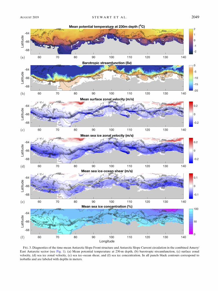
FIG. 3. Diagnostics of the time-mean Antarctic Slope Front structure and Antarctic Slope Current circulation in the combined Amery/

East Antarctic sector (see Fig. 1). (a) Mean potential temperature at 230-m depth, (b) barotropic streamfunction, (c) surface zonal

velocity, (d) sea ice zonal velocity, (e) sea ice–ocean shear, and (f) sea ice concentration. In all panels black contours correspond to

isobaths and are labeled with depths in meters.


um5 ut,e, u

e5 ut 2 ut,e, u

t5 u2 ut . (7)

Here we use dt,e as a shorthand for successive applica-

tion of tidal and eddy averaging, that is, dte. Averages of

quadratic products can also be written exactly as a sum

of mean, eddy, and tidal components. For example, the

kinetic energy can be decomposed as

1

2u2

t,e

|fflffl{zfflffl}KE

51

2u2m|ffl{zffl}

MKE

11

2u2e

e

|ffl{zffl}EKE

11

2u2t

t,e

|fflffl{zfflffl}TKE

. (8)

The depth averages of the mean, eddy, and tidal kinetic

energies (MKE, EKE, and TKE, respectively) are plotted

in Fig. 5. Both the MKE and EKE are continuously

FIG. 4. Various terms from (4) contributing to zonal acceleration/deceleration of the Antarctic Slope Current in the combined Amery/

EastAntarctica sector (see Fig. 1). (a),(b) Zonal ocean surface stress, (c),(d) zonal bottom frictional stress, (e),(f) zonal acceleration due to

mean vorticity advection and vertical advection, (g),(h) zonal acceleration due to eddy vorticity advection and vertical advection, and

(i),(j) zonal acceleration due to tidal vorticity advection and vertical advection. (left) Maps of the depth-integrated acceleration terms

and (right) the corresponding zonal-mean accelerations as functions of latitude only. In all panels black contours correspond to isobaths

and are labeled with depths in meters.


elevated along the continental slope (note the logarithmic

color scale), while the TKE is elevated over localized re-

gions of the shelf break. Thus, interactions between eddies

and the mean flow may be expected to occur along the

length of the ASC, while interactions between tides and

the mean flow may be expected to be more spatially lo-

calized (see section 3c).

There are several caveats to this decomposition:

(i) A temporal separation into subdaily and superdaily

frequencies does not exactly distinguish between

tidal and eddy fluctuations. However, more accu-

rate approaches such as tidal harmonic analysis

(Foreman and Henry 1989) were impractical due

to the very large volume of model output. For a

more detailed discussion on this issue, the reader is

referred to Stewart et al. (2018), who also quantify

the effectiveness of the daily averaging as a tidal

filter using spectral analysis. The qualitative differ-

ences in the distributions of EKE and TKE, and in

the contributions of eddies and tides to the momen-

tum budget (see section 3), also support our approx-

imate decomposition.

(ii) In practice we compute ut using 6-hourly snap-

shots of the model state. Output is available

at hourly intervals, but using higher frequencies

would impose a substantial additional computa-

tional burden, even for operations as simple

as time averaging, again due to the very large

volume of output data (Stewart et al. 2018). In

appendix B we show that using higher-frequency

output yields only small (,10%) changes in the

contributions to the momentum budget due to

transient flows.

(iii) The eddy component includes all variability with

frequencies longer than one day, including the

seasonal cycle. In appendix C we show that the eddy

momentum forcing terms discussed below are almost

identical when averaged over different seasons.

We now apply our mean/eddy/tidal decomposition to

the vorticity advection and vertical advection terms in

the depth-integrated momentum equation (4) to per-

form a preliminary examination of their role in driving

the ASC. We write each term as a sum of mean, eddy,

and tidal components as follows:

2z3 hzui|fflfflfflfflfflfflffl{zfflfflfflfflfflfflffl}Vorticity advection

52z3 hzmumi|fflfflfflfflfflfflfflfflfflffl{zfflfflfflfflfflfflfflfflfflffl}

Mean

2z3 hzeue

ei|fflfflfflfflfflfflfflfflffl{zfflfflfflfflfflfflfflfflffl}Eddy

2z3 hztut

t,ei|fflfflfflfflfflfflfflfflfflffl{zfflfflfflfflfflfflfflfflfflffl}Tidal

,

(9)

and

FIG. 5. An illustration of our mean/eddy/tidal decomposition using the depth-averaged kinetic energy [see (8)] in the combined

Amery/East Antarctica sector (see Fig. 1). (a) Mean, (b) eddy, and (c) tidal components on a logarithmic scale. In all panels black

contours correspond to isobaths and are labeled with depths in meters.


2

�w›u

›z

�|fflfflfflfflfflffl{zfflfflfflfflfflffl}

Vertical advection

52

�w

m

›um

›z

�|fflfflfflfflfflfflfflfflffl{zfflfflfflfflfflfflfflfflffl}

Mean

2

*w

e

›ue

›z

e+

|fflfflfflfflfflfflfflfflffl{zfflfflfflfflfflfflfflfflffl}Eddy

2

*w

t

›ut

›z

t,e+

|fflfflfflfflfflfflfflfflfflffl{zfflfflfflfflfflfflfflfflfflffl}Tidal

.

(10)

Figures 4e, 4g, and 4i show the total advective acceleration

of the ASC due to mean flows, eddies, and tides, respec-

tively. The qualitative spatial distributions of these terms

resemble their counterparts in Fig. 5. However, the roles

of these terms in accelerating the core of the ASC are

difficult to discern. The zonal averages shown in Figs. 4f,

4h, and 4j also obscure the ASC because the latitude of

the shelf break varies substantially across this sector.

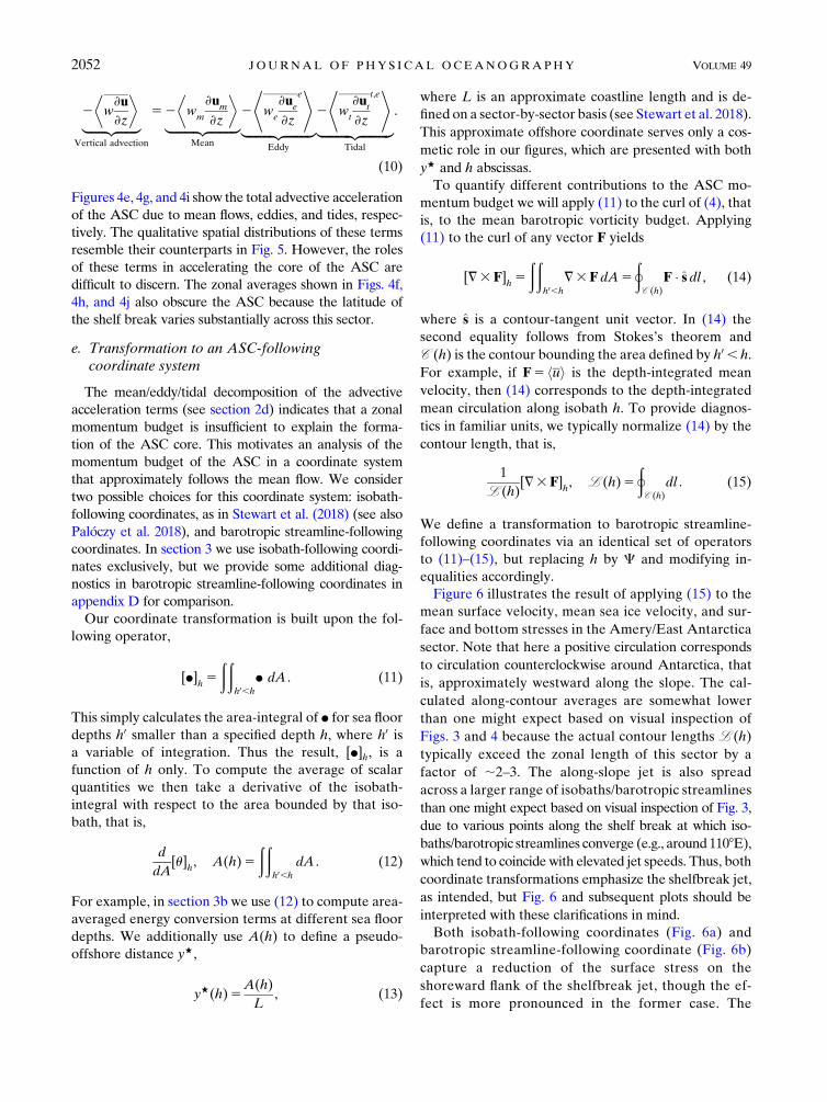
e. Transformation to an ASC-followingcoordinate system

The mean/eddy/tidal decomposition of the advective

acceleration terms (see section 2d) indicates that a zonal

momentum budget is insufficient to explain the forma-

tion of the ASC core. This motivates an analysis of the

momentum budget of the ASC in a coordinate system

that approximately follows the mean flow. We consider

two possible choices for this coordinate system: isobath-

following coordinates, as in Stewart et al. (2018) (see also

Palóczy et al. 2018), and barotropic streamline-following

coordinates. In section 3 we use isobath-following coordi-

nates exclusively, but we provide some additional diag-

nostics in barotropic streamline-following coordinates in

appendix D for comparison.

Our coordinate transformation is built upon the fol-

lowing operator,

[d]h5

ððh0,h

d dA . (11)

This simply calculates the area-integral of d for sea floor

depths h0 smaller than a specified depth h, where h0 isa variable of integration. Thus the result, [d]h, is a

function of h only. To compute the average of scalar

quantities we then take a derivative of the isobath-

integral with respect to the area bounded by that iso-

bath, that is,

d

dA[u]

h, A(h)5

ððh0,h

dA . (12)

For example, in section 3b we use (12) to compute area-

averaged energy conversion terms at different sea floor

depths. We additionally use A(h) to define a pseudo-

offshore distance y+,

y+(h)5A(h)

L, (13)

where L is an approximate coastline length and is de-

fined on a sector-by-sector basis (see Stewart et al. 2018).

This approximate offshore coordinate serves only a cos-

metic role in our figures, which are presented with both

y+ and h abscissas.

To quantify different contributions to the ASC mo-

mentum budget we will apply (11) to the curl of (4), that

is, to the mean barotropic vorticity budget. Applying

(11) to the curl of any vector F yields

[=3F]h5

ððh0,h

=3FdA5

þC (h)

F � s dl , (14)

where s is a contour-tangent unit vector. In (14) the

second equality follows from Stokes’s theorem and

C (h) is the contour bounding the area defined by h0 , h.

For example, if F5 hui is the depth-integrated mean

velocity, then (14) corresponds to the depth-integrated

mean circulation along isobath h. To provide diagnos-

tics in familiar units, we typically normalize (14) by the

contour length, that is,

1

L (h)[=3F]

h, L (h)5

þC (h)

dl . (15)

We define a transformation to barotropic streamline-

following coordinates via an identical set of operators

to (11)–(15), but replacing h by C and modifying in-

equalities accordingly.

Figure 6 illustrates the result of applying (15) to the

mean surface velocity, mean sea ice velocity, and sur-

face and bottom stresses in the Amery/East Antarctica

sector. Note that here a positive circulation corresponds

to circulation counterclockwise around Antarctica, that

is, approximately westward along the slope. The cal-

culated along-contour averages are somewhat lower

than one might expect based on visual inspection of

Figs. 3 and 4 because the actual contour lengths L (h)

typically exceed the zonal length of this sector by a

factor of ;2–3. The along-slope jet is also spread

across a larger range of isobaths/barotropic streamlines

than one might expect based on visual inspection of Fig. 3,

due to various points along the shelf break at which iso-

baths/barotropic streamlines converge (e.g., around 1108E),which tend to coincide with elevated jet speeds. Thus, both

coordinate transformations emphasize the shelfbreak jet,

as intended, but Fig. 6 and subsequent plots should be

interpreted with these clarifications in mind.

Both isobath-following coordinates (Fig. 6a) and

barotropic streamline-following coordinate (Fig. 6b)

capture a reduction of the surface stress on the

shoreward flank of the shelfbreak jet, though the ef-

fect is more pronounced in the former case. The


differences arise, in part, because the streamlines drift

across the slope slightly, typically descending ;200m

as the flow travels westward across this sector. Below

we adopt isobath-following coordinates for our analysis

because they better isolate the surface stress reduction on

the shoreward flank of the shelfbreak jet and because

barotropic streamline-following coordinates are not

well defined in other sectors of the Antarctic margins. In

appendix D we discuss these technical issues further and

show that the along-streamline circulation budget yields

qualitatively similar results to the along-isobath cir-

culation budget discussed in section 3a.

3. Along-slope acceleration of the ASC

In section 2 we described the LLC_4320 simulation

and the analysis techniques required to diagnose the

momentum balance of the ASC, namely our mean/

eddy/tidal decomposition of the LLC_4320 model

output variables and a transformation to isobath-

following coordinates. We now apply these tech-

niques to distinguish different inputs to the ASC’s

circulation and energy budgets in the Amery/East

Antarctica sector (see Fig. 1). We then examine the

vertical and along-slope localization of these inputs

and their variations between different sectors of the

Antarctic margins.

a. Circulation budget

In section 2e we showed that a transformation to

isobath-following coordinates captures the circulation

and surface/bottom stresses along the shelfbreak jet. To

distinguish different drivers of this circulation, we apply

(14) to (4),

"þC (h)

hui � s dl#t|fflfflfflfflfflfflfflfflfflfflfflfflffl{zfflfflfflfflfflfflfflfflfflfflfflfflffl}

Tendency

’2

þC (h)

f hui � n dl|fflfflfflfflfflfflfflfflfflfflfflfflffl{zfflfflfflfflfflfflfflfflfflfflfflfflffl}Coriolis

2

þC (h)

hzui � n dl2þC (h)

�w›u

›z

�� s dl|fflfflfflfflfflfflfflfflfflfflfflfflfflfflfflfflfflfflfflfflfflfflfflfflfflfflfflfflfflfflfflfflfflffl{zfflfflfflfflfflfflfflfflfflfflfflfflfflfflfflfflfflfflfflfflfflfflfflfflfflfflfflfflfflfflfflfflfflffl}

Advection

2

þC (h)

�›f

›l

�� s dl|fflfflfflfflfflfflfflfflfflfflfflfflfflfflffl{zfflfflfflfflfflfflfflfflfflfflfflfflfflfflffl}

Pressure gradient

2

þC (h)

�›

›lKE

�� s dl|fflfflfflfflfflfflfflfflfflfflfflfflfflfflfflfflfflffl{zfflfflfflfflfflfflfflfflfflfflfflfflfflfflfflfflfflffl}

KE gradient

1

þC (h)

tjz50

� s dl|fflfflfflfflfflfflfflfflfflfflfflfflfflffl{zfflfflfflfflfflfflfflfflfflfflfflfflfflffl}Surface stress

2

þC (h)

tjz52h

� s dl|fflfflfflfflfflfflfflfflfflfflfflfflfflfflffl{zfflfflfflfflfflfflfflfflfflfflfflfflfflfflffl}Bottom stress

, (16)

where n is a contour-normal unit vector. This equation

constitutes a budget for the circulation along the contour

C (h) for each isobath h. This ismathematically equivalent

to (and is calculated as) amean barotropic vorticity budget

integrated over the area bounded by the contour C (h).

Here we have neglected the tidal potential term from (4)

FIG. 6. Circulation and forcing of theAntarctic SlopeCurrent in the combinedAmery/EastAntarctica sector (see

Fig. 1). The surface and sea ice circulation and the circulation tendency due to surface and bottom stresses, cal-

culated in (a) isobath coordinates and (b) barotropic streamfunction coordinates. In each panel the lower abscissa

corresponds to an approximate measure of distance from the coast (see section 2e), while the upper abscissa

corresponds to isobaths/barotropic streamlines. In each panel the dashed black line corresponds to the 1-km isobath

[calculated from the along-streamline averaged sea floor depth in (b)] and approximately separates the continental

shelf break from the continental slope.


because it is a sum of oscillatory functions with periods on

the order of one day, and so vanishes approximately un-

der an average over the length of the simulation. Note

that we have also neglected contributions due to viscosity

under the assumption that they are small compared to the

frictional bottom stress, formulated as a quadratic drag,

but insufficient model diagnostics are provided to test this

assumption directly.

Of the terms identified in (16), we are able to evaluate

all except for the pressure gradient. As discussed in ap-

pendix B, contributions of this term to the circulation

budget did not converge even as the model output fre-

quency was refined down to hourly frequency, perhaps

due to aliasing of fast surface waves in the bottom pres-

sure.However, neither this termnor theKEgradient term

can contribute to the circum-Antarctic circulation budget;

if h is constant around the bounding contour C (h), for

example, around the full Antarctic continent, then both

the pressure gradient and KE gradient terms vanish,þC (h)

�›f

›l

�� s dl5

þC (h)

›

›lhfi � s dl5 0: (17)

Here the first equality follows from the fact that ›h/›l5 0

by definition. However, there are local contributions

from these terms in different sectors of the continent that

compensate for one another. We therefore provide an

estimate of the pressure gradient term via a residual of

the other terms in (16), while noting that the resid-

ual may also include contributions due to viscosity and

discretization errors. Note also that because the sectors

shown in Fig. 1 each span only a subset of continental

shelf, the contour C (h) generally intersects the western

and eastern boundaries, so the area-integrated curl of (4)

includes accelerations along sections parallel to the west-

ern and eastern boundaries. However, the length of these

portions of the contour are typically around 40 times

smaller than the total contour length L (h).

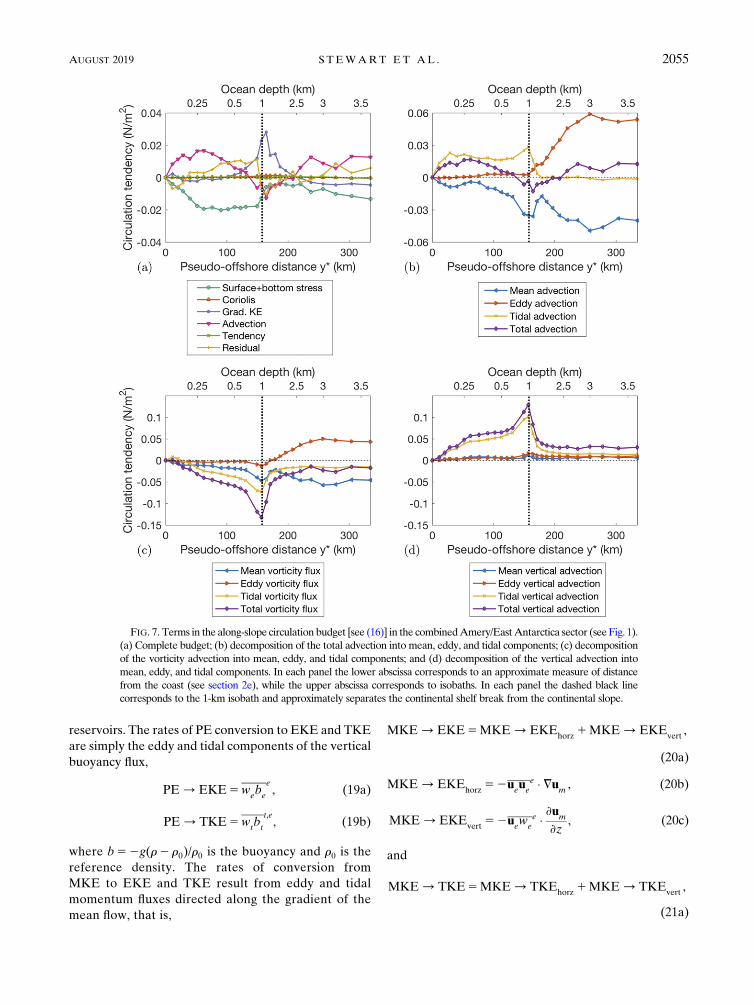
In Fig. 7 we plot the terms in (16) for the combined

Amery/East Antarctica sector (see Fig. 1). Figure 7a

shows that the net deceleration of the along-isobath cir-

culation by surface/bottom stresses is primarily balanced

by an acceleration due to the advection terms, with an

exception around the h 5 1000-m isobath where the KE

gradient term accelerates the circulation. This acceleration

coincides with a deceleration by the residual term, which

serves as an estimate of the pressure gradient accelera-

tion, and so may account for the slight offshore drift of

mean barotropic streamlines in this sector. As discussed

above, the KE gradient term cannot induce any net

circumpolar along-isobath acceleration, so we focus on

the advection terms. Figure 7b shows that the advective

acceleration of the flow is due to eddies offshore of the

shelf break (h’ 1000m) and due to tides shoreward of

the shelf break, while mean advection decelerates the

flow along all isobaths. Figures 7c and 7d show that the

mean and eddy components of the advection terms are

almost entirely due to vorticity advection, while the tidal

component results from a compensation of accelera-

tion by tidal vertical advection and deceleration by tidal

vorticity advection. Taken together, the diagnostics

shown in Figs. 6 and 7 indicate that the circulation

shoreward of the shelf break is primarily a result of tidal

acceleration (e.g., Chen and Beardsley 1995), whereas

over the continental slope both eddy vorticity fluxes and

surface stress accelerate the ASC.

b. Energy budget

While the circulation budget discussed in section

3a identified distinct roles for eddies and tides in

accelerating the ASC, the partitioning of these ac-

celerations between vorticity advection and vertical

advection leaves their interpretation somewhat am-

biguous. We therefore diagnose conversions to and

from the mean, eddy, and tidal energy reservoirs [see

(8)], which also serves to corroborate the results of

our circulation budget.

In Fig. 8 we plot a limited subset of the energy sources

and sinks that appear in the full mean/eddy/tidal energy

budget, which is presented in appendix E. Motivated by

the results of section 3a, we compare energy inputs due

to surface forcing with conversions to and from the

MKE and potential energy (PE) reservoirs. The vertical

energy flux associated with the vertical stress term in (1)

can be composed exactly as

F(t)MKE 5 u

m� tt,e, (18a)

F(t)EKE 5 u

e� tte, and (18b)

F(t)TKE 5 u

t� tt,e. (18c)

Figure 8a shows the result of evaluating these fluxes at

both z5 0 and z52h, and then applying our along-

isobath averaging operator (12) to the result. The mean,

eddy, and tidal surface energy fluxes consistently serve

to increase the MKE, EKE, and TKE, respectively,

while the bottom energy fluxes decrease them.Unlike the

mean along-slope stress (see Fig. 6), themean component

of the surface energy flux does not exhibit an obvious

minimum shoreward of the shelf break. This implies a

nonzero correlation between the mean along-isobath

flow and the mean along-isobath stress as a function

of l, the along-isobath coordinate (see section 3c).

In Figs. 8b–8d we plot the along-isobath average (12)

of the energy conversions to and from the MKE and PE


reservoirs. The rates of PE conversion to EKE and TKE

are simply the eddy and tidal components of the vertical

buoyancy flux,

PE/EKE5webe

e, (19a)

PE/TKE5wtbt

t,e, (19b)

where b52g(r2 r0)/r0 is the buoyancy and r0 is the

reference density. The rates of conversion from

MKE to EKE and TKE result from eddy and tidal

momentum fluxes directed along the gradient of the

mean flow, that is,

MKE/EKE5MKE/EKEhorz

1MKE/EKEvert

,

(20a)

MKE/EKEhorz

52ueuee � =u

m, (20b)

MKE/EKEvert

52uew

ee � ›um

›z, (20c)

and

MKE/TKE5MKE/TKEhorz

1MKE/TKEvert

,

(21a)

FIG. 7. Terms in the along-slope circulation budget [see (16)] in the combinedAmery/EastAntarctica sector (seeFig. 1).

(a) Complete budget; (b) decomposition of the total advection into mean, eddy, and tidal components; (c) decomposition

of the vorticity advection into mean, eddy, and tidal components; and (d) decomposition of the vertical advection into

mean, eddy, and tidal components. In each panel the lower abscissa corresponds to an approximate measure of distance

from the coast (see section 2e), while the upper abscissa corresponds to isobaths. In each panel the dashed black line

corresponds to the 1-km isobath and approximately separates the continental shelf break from the continental slope.


MKE/TKEhorz

52ututt,e � =u

m, (21b)

MKE/TKEvert

52utw

tt,e � ›um

›z. (21c)

We have separated these energy conversions into hori-

zontal and vertical components, associated with the

horizontal and vertical components of the eddy/tidal

momentum fluxes.

Figure 8b shows that the energy conversions are domi-

nated by exchanges between the mean, eddy, and tidal

KE reservoirs: there is a relatively weak (;1023Wm22)

PE/EKE conversion across the continental shelf and

slope, suggesting weak baroclinic eddy generation, while

PE/TKE is negligibly small. Though MKE/EKE is

positive at the shelf break itself, over the continental slope

it is consistently large (;2.53 1023Wm22) and negative,

corresponding to a transfer of energy from the eddy field to

the mean flow that is consistent with the acceleration of

the mean along-isobath circulation by eddy advection in

Fig. 7b. Figure 8c shows that this term is associated almost

FIG. 8. Energy budget terms (see section 3b) averaged between isobaths in the combined Amery/East

Antarctic sector (see Fig. 1). (a) Surface/bottom energy fluxes decomposed into mean, eddy, and tidal com-

ponents. (b) EKE and TKE conversion from MKE and PE. (c) Decomposition of the MKE/EKE term

into horizontal and vertical components. (d) Decomposition of the MKE/TKE term into horizontal and

vertical components. In each panel, the lower abscissa corresponds to an approximate measure of distance from

the coast (see section 2e) while the upper abscissa corresponds to isobaths. In each panel the dashed black

line corresponds to the 1-km isobath and approximately separates the continental shelf break from the

continental slope.


entirely with horizontal eddy momentum fluxes over the

continental slope, lending support to our interpretation of

the eddy forcing of the circulation as an eddy-momentum

flux convergence in section 3a. The MKE/TKE term

in Fig. 8b is consistently large (;2.5 3 1023Wm22) and

negative over the continental shelf, consistent with the

acceleration of the mean along-isobath circulation by tidal

acceleration in Fig. 7b. Figure 8d shows that this tidal

production of MKE is primarily associated with vertical

momentum fluxes up the vertical gradient of the mean

momentum.

c. Along-slope localization

The diagnostics presented in section 3a and section 3b

encompass the entire Amery/East Antarctica sector, yet

Figs. 3 and 4 suggest that there are substantial along-slope

variations in the structure and forcing of the ASC’s shelf-

break jet. In Fig. 9 we plot along-slope variations of key

terms in the circulation and energy budgets. We use lon-

gitude as an approximate measure of along-slope distance,

exploiting the approximately zonal orientation of the

continental slope in this sector.We focus on the h5 300-m

isobath, along which the reduction of the along-isobath

surface stress and compensating along-isobath accelera-

tion by tides are most pronounced. Performing the same

calculation using other isobaths in the core of the ASC

(e.g., the 400- and 500-m isobaths) yields qualitatively

similar results. Similar to the method described by Stewart

et al. (2018), we define a series of zonal ‘‘windows’’ of

width 38 and centered on longitudes separated by 0.58.The ith window defines an area Ai(h) with bounding

contour C i(h) for our integration operator (11).

However, the zonal boundaries of the contour C i(h) are

no longer negligible compared to its total length (see sec-

tion 3a), so we have calculated and removed these contri-

butions in Fig. 9.

Figure 9 shows that the along-isobath flowof the sea ice

and ocean surface covary closely (Pearson’s correlation

coefficient r 5 0.92) as a function of longitude. The sea

ice–ocean shear fluctuates around zero with zonal varia-

tions on a scale of around 108, and very closely predicts

the mean surface stress (r 5 0.98),1 despite substantial

seasonal fluctuations in the monthly-mean velocities and

stresses (see appendix C). The advective acceleration of

the circulation (Fig. 9b) also exhibits substantial along-

slope variations. This is primarily due to localized

stretches of tidal advective acceleration, which are par-

tially compensated by mean advective deceleration; the

tidal and mean advective accelerations are anticorrelated

(r 5 20.54). While one might expect a relationship be-

tween stretches of reduced surface stress and along-

slope advective acceleration, they are also only weakly

correlated (r 5 20.28). Alternatively, advective ac-

celeration may be expected to reduce the ice–ocean

shear, and thus the surface stress, farther downstream,

but the two are even more weakly correlated under a

zonal lag.

Figures 9c and 9d show that the net tidal advective

acceleration results from relatively strong local acceler-

ations due to tidal vertical advection that are partially

compensated by local decelerations due to tidal vorticity

advection (r5 0.90). Figure 9e shows that MKE/TKE

is similarly localized, though there is not a clear visual

correspondence between its amplitude and that of the

net tidal advective acceleration of the circulation, and

they are relatively weakly correlated (r 520.47). The

net tidal advective acceleration may be expected to

coincide with strong tidal flows and steep slopes

(e.g., Garreau and Maze 1992; Chen and Beardsley

1995). While the tidal acceleration exhibits a relatively

weak correlation with TKE (r 5 0.46) and an in-

significant correlation with topographic slope (r520.18,

p 5 0.02), it is strongly correlated with their product

(r5 0.68), consistent with the scalings of Brink (2011)

for topographically rectified flows. In summary, while

tidal acceleration of the ASC is evidently strongly

localized as a function of along-slope distance, the

extent to which it controls along-slope variations in

the ASC speed and ice–ocean shear remains somewhat

ambiguous.

d. Vertical structure and overturning

Thus far we have only discussed depth-integrated

contributions to the along-slope circulation and energy

budgets. We now address the vertical structure of the

along-isobath circulation forcing, focusing on the con-

tribution of the advection terms in (1) on the cross-

isobath mean overturning circulation.

Figure 10 shows the Eulerian-mean overturning

circulation diagnosed in our isobath-following co-

ordinate system. We define the mean overturning

streamfunction as

cm(h, z)[

ð0z

dz0þC (h)

um� ndl , (22)

where z0 is a variable of integration. In Fig. 10 we plot

eddy and tidal overturning streamfunctions estimated

via an extended Transformed Eulerian Mean formula-

tion, described by Stewart et al. (2018) and omitted

here in the interest of brevity. Note that these stream-

functions are estimates of the overturning due to the

1Unless stated explicitly, the p values corresponding to these

correlation coefficients are all smaller than 1023.


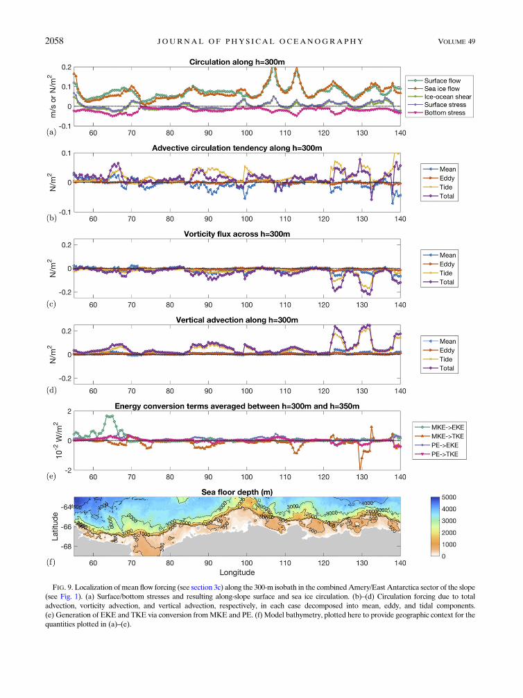
FIG. 9. Localization of mean flow forcing (see section 3c) along the 300-m isobath in the combinedAmery/East Antarctica sector of the slope

(see Fig. 1). (a) Surface/bottom stresses and resulting along-slope surface and sea ice circulation. (b)–(d) Circulation forcing due to total

advection, vorticity advection, and vertical advection, respectively, in each case decomposed into mean, eddy, and tidal components.

(e) Generation of EKE and TKE via conversion fromMKE and PE. (f) Model bathymetry, plotted here to provide geographic context for the

quantities plotted in (a)–(e).


generalized Stokes’ drift associated with eddies and

tides, and are distinguished from the eddy- and tidal-

driven components of the mean overturning circulation

discussed below. There is an approximate compensation

between a relatively intense counterclockwise mean

overturning across the shelf and shelf break in Fig. 10a,

and clockwise tidal overturning of similar magnitude in

Fig. 10c. Stewart et al. (2018) showed that advection

of along-isobath mean potential temperature by these

streamfunctions largely accounted for the diagnosed

mean and tidal heat fluxes across the shelf and shelf

break.

FIG. 10. Vertical structure of the along-slope circulation forcing (see section 3d), visualized via its contributions to the mean

overturning circulation in the combined Amery/East Antarctica sector (see Fig. 1). (a)–(c) Components of the overturning circu-

lation associated with the time-mean flow, approximate eddy Stokes’ drift, and approximate tidal Stokes’ drift, calculated

following Stewart et al. (2018). (d)–(g) Estimated contributions to the mean overturning circulation due to mean advection, eddy

advection, tidal advection, and surface stress, respectively. (h) An estimate of the total mean overturning circulation constructed

from (d)–(g). (i) Mean overturning circulation calculated from the Coriolis force alone. By our definition of the overturning

streamfunction (22), the flow follows streamlines clockwise around red-shaded regions and counterclockwise around blue-shaded

regions.


The vanishing surface stress shoreward of the shelf

break in Fig. 6 suggests that the intense mean shelf

overturning in Fig. 10a cannot be explained by

Ekman transport. We therefore now consider the

possibility that this overturning results from advec-

tive acceleration by transient flows, which have been

shown to produce mean overturning circulations,

for example, in the ACC’s jets (Li et al. 2016) and

in idealized simulations of ASC jets (Stewart and

Thompson 2016). Exploiting the approximately zonal

orientation of the continental slope in the Amery/

East Antarctica sector, and correspondingly small

variation in the Coriolis parameter f over this region,

we write

cm’

1

f0

ð0z

dz

(þC (h)

fum� ndl

)|fflfflfflfflfflfflfflfflfflfflfflfflfflfflfflfflfflfflfflfflffl{zfflfflfflfflfflfflfflfflfflfflfflfflfflfflfflfflfflfflfflfflffl}

Mean overturning reconstructed from Coriolis force

521

f0

ð0z

dz

(þC (h)

zmum� ndl1

þC (h)

wm

›um

›z� s dl

)|fflfflfflfflfflfflfflfflfflfflfflfflfflfflfflfflfflfflfflfflfflfflfflfflfflfflfflfflfflfflfflfflfflfflfflfflfflfflfflfflfflfflfflfflffl{zfflfflfflfflfflfflfflfflfflfflfflfflfflfflfflfflfflfflfflfflfflfflfflfflfflfflfflfflfflfflfflfflfflfflfflfflfflfflfflfflfflfflfflfflffl}

Mean overturning due to mean advection

21

f0

ð0z

dz

8<:þC (h)

zeue

e � n dl1þC (h)

we

›ue

›z

e

� s dl9=;|fflfflfflfflfflfflfflfflfflfflfflfflfflfflfflfflfflfflfflfflfflfflfflfflfflfflfflfflfflfflfflfflfflfflfflfflfflfflfflfflfflfflfflfflffl{zfflfflfflfflfflfflfflfflfflfflfflfflfflfflfflfflfflfflfflfflfflfflfflfflfflfflfflfflfflfflfflfflfflfflfflfflfflfflfflfflfflfflfflfflffl}

Mean overturning due to eddy advection

21

f0

ð0z

dz

8<:þC (h)

ztut

t,e � n dl1þC (h)

wt

›ut

›z

t,e

� s dl9=;|fflfflfflfflfflfflfflfflfflfflfflfflfflfflfflfflfflfflfflfflfflfflfflfflfflfflfflfflfflfflfflfflfflfflfflfflfflfflfflfflfflfflfflfflfflffl{zfflfflfflfflfflfflfflfflfflfflfflfflfflfflfflfflfflfflfflfflfflfflfflfflfflfflfflfflfflfflfflfflfflfflfflfflfflfflfflfflfflfflfflfflfflffl}

Mean overturning due to tidal advection

11

f0

þC (h)

tjz50

� s dl|fflfflfflfflfflfflfflfflfflfflfflfflfflfflfflffl{zfflfflfflfflfflfflfflfflfflfflfflfflfflfflfflffl}Mean overturning due to surface stress

1 ::: . (23)

Here the second equality follows from taking a vertical in-

tegral of (1) and rearranging, and f0 521:323 1024 rad s21

is approximately equal to the Coriolis parameter at

658S. Equation (23) states that the Coriolis force as-

sociated with the mean overturning circulation bal-

ances the along-isobath surface stress, the mean, eddy,

and tidal advective accelerations, and other terms in

the circulation budget.In Figs. 10d–g, we use (23) to decompose the mean

streamfunction into components driven by mean,

eddy, and tidal advection, and due to the surface

stress, respectively. The sum of these contributions,

shown in Fig. 10h, is qualitatively and quantitatively

similar to the diagnosed mean overturning stream-

function in Fig. 10a. The differences between Figs. 10a

and 10h are due to contributions from the pressure

gradient and KE gradient terms in (4), which we have

neglected in Fig. 10 because they cannot produce

any net circumpolar acceleration. Figure 10i shows

that reconstructing the mean overturning from the

Coriolis force yields an almost identical result to

computing cm directly from the model output. The

dominant contribution to the mean overturning cir-

culation across the shelf and shelf break is due to the

along-isobath acceleration by tidal advection (;2.5Sv),

with weaker contributions from eddy advection (;0.25Sv)

and mean advection (;1 Sv). While the surface stress-

driven transport vanishes over the shelf, over the con-

tinental slope it produces a substantial (;1Sv) mean

overturning. However, in this sector the mean over-

turning due to eddy advection (;4 Sv) dominates over

the lower slope (isobaths deeper than h 5 2500m).

Taken together, these diagnostics imply that the

mean overturning across the continental shelf and

slope is much stronger than might be expected

due to the surface winds alone, being enhanced due

to along-slope advective acceleration by transient

flows.

e. Circum-Antarctic regional variations

The previous subsections have all described results

diagnosed from the Amery/East Antarctica sector. To

determine the generality of these results, we now ex-

tend our diagnostics to all of the regions identified in

Fig. 1. The continental slope undergoes substantial

meridional excursions in some sectors, particularly the

Weddell and West Antarctic Peninsula (WAP). This

makes an assessment of, for example, the along-slope

localization of terms in the circulation and energy

budgets more challenging at the circum-Antarctic

scale. We therefore focus on the key circulation

budget terms identified in section 3a. As discussed in

section 2, we exclude the Amundsen and Belling-

shausen sectors from our analysis due to qualitative

differences between the model’s bathymetry and the

ocean’s.

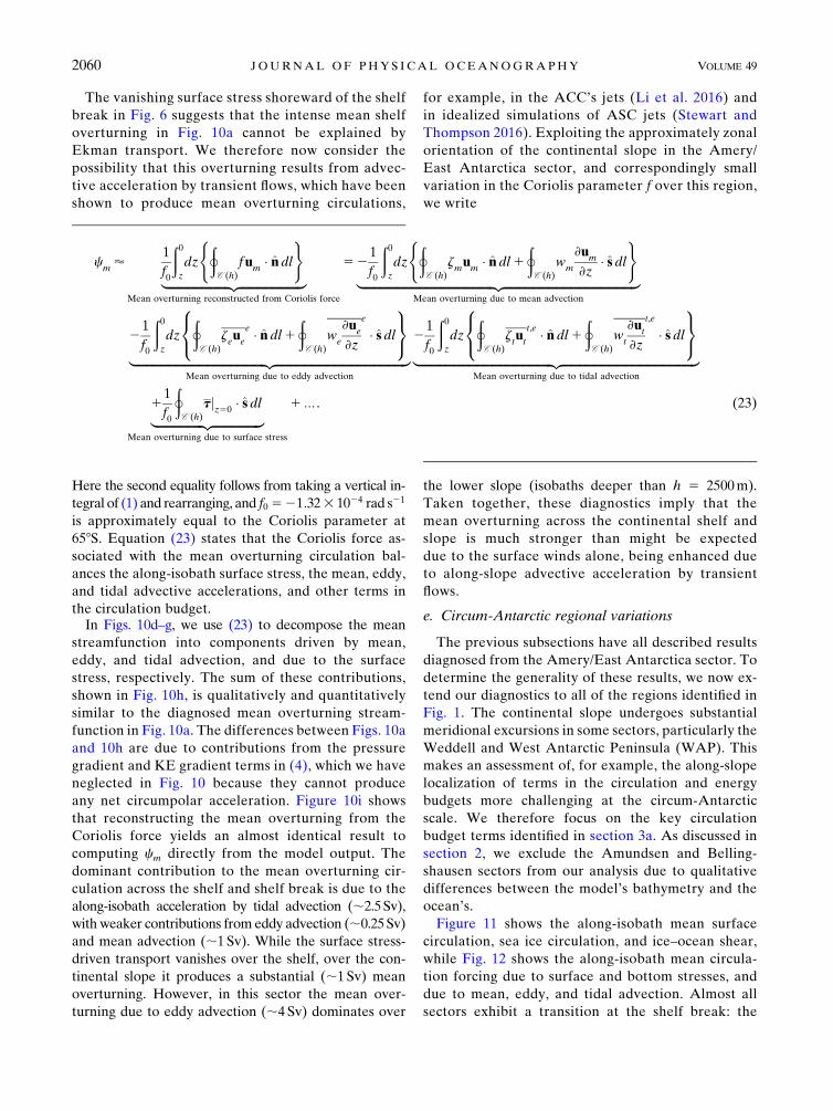
Figure 11 shows the along-isobath mean surface

circulation, sea ice circulation, and ice–ocean shear,

while Fig. 12 shows the along-isobath mean circula-

tion forcing due to surface and bottom stresses, and

due to mean, eddy, and tidal advection. Almost all

sectors exhibit a transition at the shelf break: the


ice–ocean shear (Fig. 11) and surface stress (Fig. 12)

vanish shoreward of the shelf break, where tides

accelerate the ASC. An exception is the Weddell,

in which the ASC experiences acceleration due to

tidal advection and deceleration due to the surface

stress across the entire continental shelf and slope.

This is likely due to perennial ice cover and strong

tides in this sector (Robertson 2001); our seasonal

decomposition of the Amery/East Antarctic sector in

appendix C also shows negative surface stresses in

winter, when the ice cover is thick. Figure 12 also

highlights that acceleration of the ASC by eddies

over the continental slope varies widely between

different sectors, with magnitudes ranging from around

FIG. 11. (a)–(h) Comparison of along-slope circulation in all eight sectors of the Antarctic margins identified

in Fig. 1. In each panel the lower abscissa corresponds to an approximate measure of distance from the coast

(see section 2e), while the upper abscissa corresponds to isobaths. Dashed lines are used in (g) and (h) to emphasize

that the model’s bathymetry differs qualitatively from the ocean’s in these regions, as discussed in section 2. In each

panel the dashed black line corresponds to the 1-km isobath and approximately separates the continental shelf

break from the continental slope.


0.14Nm22 in the WAP sector to approximately zero in

the Weddell.

4. Discussion and conclusions

a. Summary of results

In this study we have used a high-resolution global sim-

ulation, the LLC_4320, to investigate the role of transient

flows in driving the ASC, and in particular the ASC’s

shelfbreak jet. The model ASC is accelerated by a

westward surface stress that is ultimately input by the

coastal easterly winds, but must be transferred to the

ocean via the overlying sea ice over much of the year,

consistent with previous studies (e.g., Mathiot et al.

2011; Heywood et al. 2014). The imbalance between

surface zonal stress and bottom frictional stress (Fig. 4)

suggests that the zonal surface momentum input is

primarily balanced by topographic form stress, as in the

ACC (e.g., Munk and Palmén 1951; Stewart and Hogg

2017). However, we are unable to verify this force

balance directly from the model, as discussed in

appendix B.

A central result of this study (summarized in Fig. 13)

is that the shelfbreak jet, which is typically tens of

FIG. 12. As in Fig. 11, but instead showing terms in the along-isobath circulation budget (see section 3a).


kilometers wide and coincides with the ASF, is subject

to a qualitatively different momentum balance from

the rest of the ASC and continental shelf currents.

Here the mean westward surface stress vanishes or

even reverses (see Figs. 4 and 12). This occurs where

the mean surface ocean flow speed approaches or

exceeds that of the overlying sea ice (see Figs. 3, 6,

and 9). This suggests that an additional source of

along-slope acceleration, due, for example, to tran-

sient momentum flux convergence by eddies (e.g.,

Stewart and Thompson 2016; Li et al. 2016) or tides

(Garreau and Maze 1992; Chen and Beardsley 1995).

We therefore approximately decomposed the model

output into mean, eddy, and tidal components (section

2d) to identify their relative contributions to driving

the along-shelfbreak circulation, and posed our anal-

ysis in an isobath-following coordinate system that

emphasizes the shelfbreak jet.

Applying this analysis framework to the LLC_4320

simulation in section 3 revealed that the shelfbreak jet is

primarily accelerated westward by tidal vertical advec-

tion, partially compensated by deceleration due to tidal

vorticity advection [see (4)]. This acceleration is collo-

cated with a conversion from TKE to MKE via tidal

vertical momentum fluxes (see Fig. 8), suggesting that

this might be interpreted as the result of vertical mo-

mentum flux convergence by tides at the shelf break.

The tidal acceleration is localized along the shelf break

(Fig. 9), typically coinciding with stretches of steep

continental slope and high TKE, consistent with the

phenomenology of tidal rectification (Garreau and

Maze 1992; Chen and Beardsley 1995). In section 3d we

showed that the mean overturning circulation across the

shelf break is also primarily driven by tidal acceleration

(Fig. 10). Thus, while previous studies have highlighted

the importance of tides for the ASC in specific regions

FIG. 13. Schematic illustrating the roles of wind, sea ice, eddies, and tides in accelerating the ASC. Over the continental slope,

momentum is primarily sourced from the winds via the sea ice. The resulting shoreward Ekman transport and associated over-

turning circulation is compensated by an opposing eddy overturning circulation that serves to restratify the water column, anal-

ogous to the long-standing paradigm for the ACC (Karsten and Marshall 2002; Marshall and Radko 2003). At the shelf break, tides

accelerate the ASC to the point that the surface speed is typically comparable to that of the overlying sea ice, resulting in an

approximate vanishing of the surface momentum input. Consequently, tidal acceleration drives the mean shoreward surface

transport and associated overturning circulation, with tidal Stokes’ drift providing the opposing, restratifying overturning

circulation.


(e.g., Robertson 2001; Flexas et al. 2015), our findings

indicate that tides serve as a primary driver of the along-

slope circulation andmean overturning of the ASF in all

sectors of the Antarctic margins considered in this study

(Fig. 12).

While we found a relatively minor role for eddies at

the shelf break, in the Amery/East Antarctica sector

they produce a substantial acceleration of the ASC over

the continental slope. These accelerations coincide with

conversion from EKE to MKE via horizontal momen-

tum fluxes directed up the mean momentum gradient

(Fig. 8), suggesting that they can be interpreted as eddy

horizontal momentum flux convergence forcing the

mean flow (e.g., Stewart and Thompson 2016; Li et al.

2016). It is not clear from our diagnostics why eddies

drive the mean flow, rather than vice versa, but we

speculate that the mechanism is topographic rectifica-

tion of quasigeostrophic flows (e.g., Brink 2016; Wang

and Stewart 2018). In contrast to the tidal acceleration of

the shelfbreak jet, the eddy acceleration of the slope

current is less consistent between different sectors of the

Antarctic margins (Fig. 12). This may be a consequence

of variations in the EKE over the continental slope,

perhaps due to varying proximities of the continental

slope to the energetic ACC to the north.

b. Implications and outlook

Together the above results imply that the ASC’s

shelfbreak current is accelerated by tidal rectification to

the extent that the ocean is only weakly accelerated

westward by the sea ice, if at all (e.g., Fig. 6). Indeed, our

analysis in appendix C suggests that over the course of a

year, the shelfbreak jet may cycle through states in which

it is accelerated by winds, weakly accelerated by the

overlying sea ice, or acting to accelerate the sea ice, while

in all seasons experiencing approximately the same tidal

acceleration. Theoretical or comprehensivemodels of the

ASC that exclude the effects of tides therefore likely

underrepresent the strength of the shelfbreak jet associ-

ated with the ASF (Fig. 3), and so may underestimate

ocean and sea ice transport around Antarctica. Further-

more such models would not capture the dominance of

the tides in driving the cross-shelf overturning circula-

tion (Fig. 10), which transports surface waters shoreward

and acts to steepen isopycnals in the ASF. Various pre-

vious studies have emphasized the role of the wind in

transporting surface waters across the continental shelf

break (see, e.g., Nøst et al. 2011; Stewart and Thompson

2012; Spence et al. 2014; Zhou et al. 2014; Greene et al.

2017; Paolo et al. 2018). Further work will be required to

FIG. A1. Evaluation of (b),(d) the modeled annual-mean Antarctic Slope Front/Current against

(a),(c) observations made in February 2007 during the ADELIE cruise in the northwestern Weddell Sea (see

Thompson and Heywood 2008). (top) Potential temperature (colors) and neutral density (black contours)

calculated following Jackett and McDougall (1997). Labels indicate neutral densities on each isopycnal

(kg m23). (bottom) Zonal velocity contoured every 0.01 m s21 (colors) and 0.04 m s21 (black contours). In

(a) and (c) the dashed black lines indicate locations at which CTD cast and lowered ADCP measurements

were taken.


determine how tides modify the response of the

ASC to wind variability (e.g., Armitage et al. 2018)

and to historical and future wind trends (Hazel and

Stewart 2019).

While the LLC_4320 simulation’s high spatial res-

olution and output frequency make it well suited

to the analysis of eddy and tidal dynamics at the

Antarctic margins (Padman et al. 2009; Stewart and

Thompson 2015b), it carries several substantial ca-

veats. For example, we were unable to diagnose

pressure forces directly, requiring that we infer them

approximately as a residual of other terms (Fig. 7).

While no net along-isobath pressure force is possi-

ble around the entire continent (see section 3a), we

cannot completely exclude the possibility of local

contributions that substantially influence the along-

isobath circulation budget. We have also been unable

to assess the effect of buoyancy forcing on the ASF,

due, for example, to localized inputs of freshwater

from floating ice shelves along the coast (Hattermann

et al. 2014; Hattermann 2018), which are excluded by

the LLC_4320 simulation’s simplified distribution of

continental runoff (see section 2). In addition to

changing the baroclinic structure of the ASF/ASC,

buoyancy forcing also serves to drive overturning

circulations in density space and thereby indirectly

enters the along-slope circulation budget, though its

vertically integrated contribution is zero (Stewart and

Thompson 2016).

The model’s omission of dense shelf water (DSW)

production is likely causing it to underestimate the

effect of eddies in regions such as the western Ross

andWeddell Seas, where eddies may receive more of

their energy as a result of buoyancy forcing than

wind forcing (Lane-Serff and Baines 1998; Stewart

and Thompson 2016). The export and DSW, and the

return flow of CDW and other water masses onto the

continental shelf, are therefore also absent from our

diagnostics of the overturning circulation in Fig. 10.

Due to the model’s high horizontal resolution, it

would likely simulate DSW overflows if the in-

tegration could practically be continued for a longer

period (Newsom et al. 2016; Dufour et al. 2017),

though this also raises the possibility of the stratifi-

cation and circulation drifting far from observations.

The simulation also only represents one annual re-

alization of the Antarctic atmospheric forcing sam-

pled from substantial interannual variability (e.g.,

Gordon et al. 2015; Langlais et al. 2015). The 1-yr

duration of the simulation appears to be sufficient

to avoid distortion of the eddy and tidal statistics,

based on the consistency of the eddy/tidal accel-

eration between seasons (see appendix C) and the

eddy/tidal heat transports between the 1-yr LLC_

4320 and 2-yr LLC_2160 simulations (Stewart et al.

2018). However, longer simulations at higher reso-

lution will be required to quantify drivers of sea-

sonal and interannual variations in the ASF and ASC.

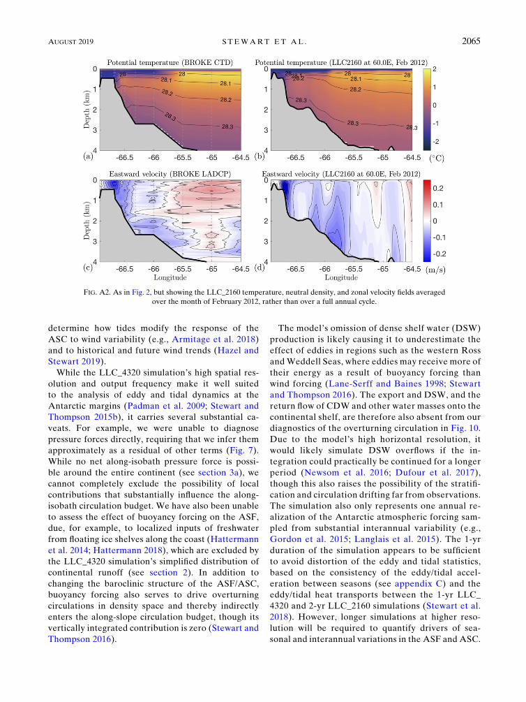
FIG. A2. As in Fig. 2, but showing the LLC_2160 temperature, neutral density, and zonal velocity fields averaged

over the month of February 2012, rather than over a full annual cycle.


Finally, the model’s bathymetry product (Smith and

Sandwell 1997) differs qualitatively from the real

continental shelf and slope in the Amundsen and

Bellingshausen sectors, precluding an accurate diagnosis

of theASC’s dynamics in these sectors (see Stewart et al.

2018).

There are also various caveats to our analysis ap-

proach. Both of the coordinate transformations (iso-

bath-following and barotropic streamline-following)

discussed in section 2e produce somewhat distorted

representations of the average structure and forcing

of the shelfbreak jet and should be interpreted ac-

cordingly. As emphasized in section 2d, our ‘‘eddy’’

and ‘‘tidal’’ components only approximately corre-

spond to their representative flow phenomena,

and include other flows that evolve on comparable

time scales. For example, the effect of tides could

be more accurately isolated via tidal harmonic

analysis (Foreman and Henry 1989) and the ‘‘eddy’’

component may also include phenomena such as low-

frequency coastal-trapped waves (Kusahara and

Ohshima 2014; Spence et al. 2017) and the oceanic

response to synoptic wind variability (e.g., Davis et al.

2018). Our analysis options were strongly constrai-

ned by the computational cost of performing oper-

ations on the very large volume of model output

(see Stewart et al. 2018), a problem that might be

ameliorated in future by improved computational

infrastructure and tools for working with large data-

sets. The computational burden could further be re-

duced by conducting regional simulations of the full

Antarctic margins, which would also allow for inclu-

sion of ice shelf cavities and updated continental shelf

bathymetry.

In summary, the circum-Antarctic acceleration of

the ASC’s shelfbreak jet by tides leads to a qualita-

tively different momentum balance and mean over-

turning of the ASF than would be expected due

to winds alone (e.g., Nøst et al. 2011; Stewart and

Thompson 2016), while eddies contribute substantially

to the acceleration of the ASC in specific sectors of the

continental slope. However, the various caveats at-

tached to the LLC_4320 simulation and the limitations

of our analysis leave many open questions to be ad-

dressed in future studies. In particular, the combined

impact of DSW export and tides on the ASC may

FIG. B1. Sensitivity of circulation forcing due to (a) vorticity advection and (b) vertical advection to model

output frequency. For each panel the circulation tendency was calculated as described in section 2e for a sub-

domain of the Amery region (see Fig. 1), between 70.78 and 79.08E and between 68.38 and 65.18S. In each case we

calculated the total circulation tendency due to all transient flows, using the LLC_2160 simulation for compu-

tational efficiency.

FIG. B2. Sensitivity of circulation forcing due to pressure gradi-

ents to model output frequency. For each frequency the circulation

tendency was calculated as described in section 2e for the com-

bined Amery/East Antarctica region (see Fig. 1). These results

have been calculated using the LLC_2160 simulation for compu-

tational efficiency.


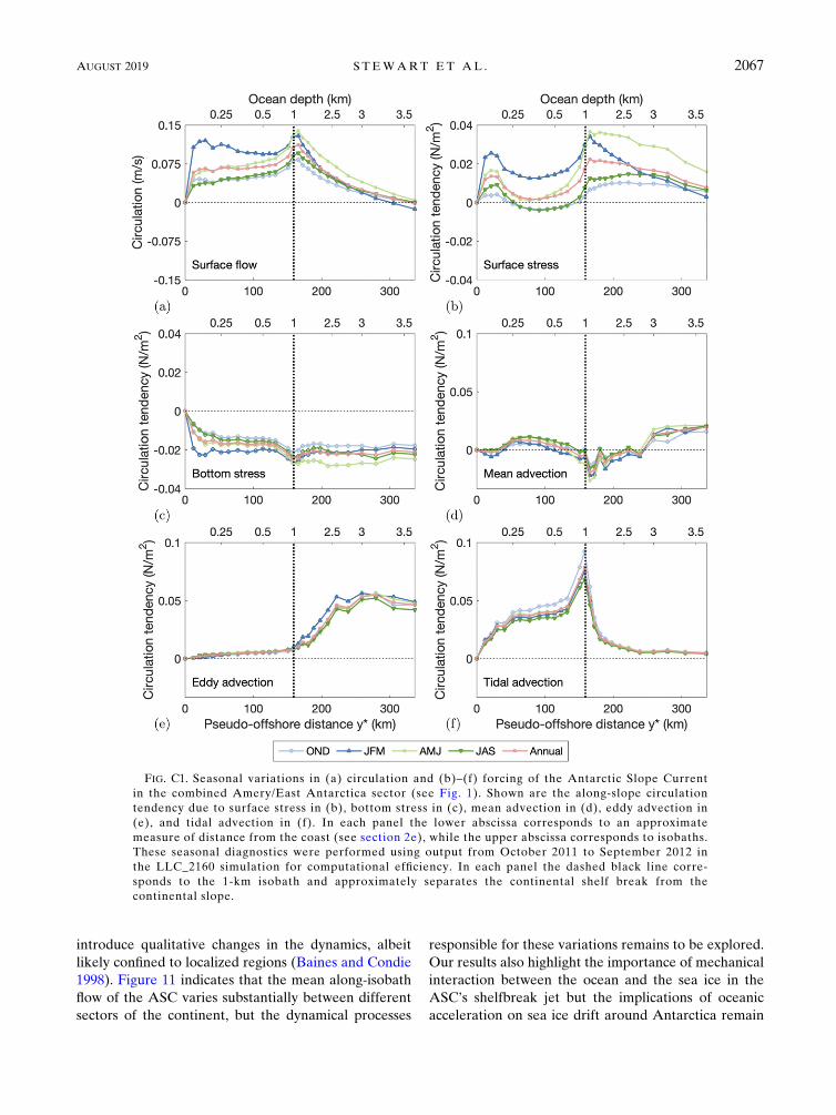
introduce qualitative changes in the dynamics, albeit

likely confined to localized regions (Baines and Condie

1998). Figure 11 indicates that the mean along-isobath

flow of the ASC varies substantially between different

sectors of the continent, but the dynamical processes

responsible for these variations remains to be explored.

Our results also highlight the importance of mechanical

interaction between the ocean and the sea ice in the

ASC’s shelfbreak jet but the implications of oceanic

acceleration on sea ice drift around Antarctica remain

FIG. C1. Seasonal variations in (a) circulation and (b)–(f) forcing of the Antarctic Slope Current

in the combined Amery/East Antarctica sector (see Fig. 1). Shown are the along-slope circulation

tendency due to surface stress in (b), bottom stress in (c), mean advection in (d), eddy advection in

(e), and tidal advection in (f). In each panel the lower abscissa corresponds to an approximate

measure of distance from the coast (see section 2e), while the upper abscissa corresponds to isobaths.

These seasonal diagnostics were performed using output from October 2011 to September 2012 in

the LLC_2160 simulation for computational efficiency. In each panel the dashed black line corre-

sponds to the 1-km isobath and approximately separates the continental shelf break from the

continental slope.


to be explored. Finally, our results offer little insight

into the sensitivity of the ASC to the modeled tidal

amplitudes, atmospheric forcing, ambient offshore

stratification, and sea floor geometry, and thus little in-

sight into past and potential future changes in the ASC.

We suggest that progress on these fronts will require

high-resolution circum-Antarctic regional modeling,

process-oriented simulations to more clearly isolate

different ASC drivers, and additional observational de-

ployments in regions of strong tidal and eddy ASC

forcing.

Acknowledgments. The authors thank Andrew

Thompson and Mar Flexas for helpful comments on

an earlier draft of this manuscript. The authors thank

Ed Doddridge and an anonymous reviewer for many

detailed recommendations that improved the manu-

script. This material is based in part upon work sup-

ported by the National Science Foundation under

Grant Numbers OCE-1538702, ANT-1543388, and

OCE-1751386. This research was supported under

the Australian Research Council’s Special Research

Initiative Antarctic Gateway Partnership (Project ID

FIG. D1. Terms in the along-flow circulation budget in the combined Amery/East Antarctica sector (see Fig. 1).

(a) Complete budget; (b) decomposition of the total advection into mean, eddy, and tidal components;

(c) decomposition of the vorticity advection into mean, eddy, and tidal components; and (d) decomposition of

the vertical advection into mean, eddy, and tidal components. In each panel the lower abscissa corresponds to

an approximate measure of distance from the coast (see section 2e), while the upper abscissa corresponds to

barotropic streamlines. In each panel the dashed black line corresponds to the 1-km isobath (calculated via the

along-streamline averaged sea floor depth) and approximately separates the continental shelf break from the

continental slope.


SR140300001). DM carried out this work at the Jet

Propulsion Laboratory (JPL), California Institute of

Technology, under a contract with the National

Aeronautics and Space Administration (NASA). The

authors thank Andrew Thompson and Karen Hey-

wood for providing the observational data used to

create Fig. A1. High-end computing resources were

providedby theNASAAdvancedSupercomputing (NAS)

Division of theAmes Research Center. The authors thank

the MITgcm development team, NAS computer sci-

entists, and SGI engineers for their contributions to

producing and making available the high-resolution

model output used in this study. Themodel configuration

files can be downloaded from: http://wwwcvs.mitgcm.org/

viewvc/MITgcm/MITgcm_contrib/llc_hires/llc_4320/.

The raw model output data are stored on NASA’s

Pleiades supercomputer and may be accessed via

request to DM. The model analysis used the Extreme

Science and Engineering Discovery Environment

(XSEDE; Towns et al. 2014), which is supported by

National Science Foundation Grant ACI-1548562.

The time-averaged model output fields used to de-

rive the results presented in this manuscript can

be downloaded from: https://doi.org/10.4226/77/

5a37035ea15b2.

APPENDIX A

Additional Model Evaluation

Here we discuss additional evaluation of the

LLC_4320 simulation, which is limited by the paucity of

simultaneous high-resolution hydrographic and velocity

measurements across the ASC. In Fig. A1 we present

plots analogous to those shown in Fig. 2, but using ob-

servations from the ADELIE deployment (Thompson

and Heywood 2008) in the western Weddell Sea. Both

the modeled and observed meridional velocities ex-

hibit multiple, northward, primarily barotropic jets. In

this section, however, the absence of AABW in the

model leads to more substantial differences in the

stratification over the slope and shelf break, compared

to Fig. 2.

As emphasized in section 2b, quantitative agreement

between the model and observations should not be

expected because the former is an annual mean and

the latter an approximately instantaneous snapshot.

In Fig. A2 we replicate Fig. 2 using output from the

LLC_2160 simulation averaged over the month of

February 2012, rather than over a full annual cycle.

Despite comparing the model output with observations

taken in the same calendar month, Fig. A2 does not

exhibit discernibly better agreement between the mod-

eled and observed ASC states than Fig. 2.

APPENDIX B

Sensitivity to Model Output Frequency

As discussed in section 2d, all diagnostics from the

LLC_4320 simulation were calculated using 6-hourly

instantaneous model output for computational effi-

ciency, though hourly output is available. In Fig. B1

we test the sensitivity of the computed accelera-

tions due to vorticity advection and vertical advec-

tion to the frequency of the model output in a subset

of the Amery sector (see Stewart et al. 2018) in the

LLC_2160 simulation. In each case we have sub-

tracted the corresponding accelerations associated

with the time-mean, so the curves in Fig. B1 corre-

spond to the total acceleration due to all transient

flows. While there are ;100% differences in the re-

sult between output frequencies of 24 and 6 h, higher

frequencies yield only small (;10%) changes in the

computed accelerations. This is consistent with sim-

ilar results presented by Stewart et al. (2018) for the

cross-slope heat fluxes.

In section 3a we noted that we could not directly

calculate the pressure gradient term in (16). This is be-

cause, unlike all other terms in (16), the calculated

pressure gradient term does not converge under re-

finement of the model output frequency. Figure B2

shows the along-isobath circulation over the entire

Amery/East Antarctica sector in the LLC_2160 simu-

lation, calculated using several different output fre-

quencies. The differences in the acceleration between

hourly and 2-hourly output frequencies are compa-

rable to those between 4- and 6-hourly output fre-

quencies, so evidently convergence has not been

achieved. While it appears that the magnitude of the

acceleration is becoming progressively smaller, it is

not possible to accurately extrapolate to the actual

circulation forcing. We speculate that high-frequency

surface waves may be the source of this issue, which

highlights the need for online averaging in future

model studies of Antarctic tides, particularly for the

pressure field.

APPENDIX C

Seasonal Cycle

The ASC and the near-Antarctic winds exhibit a

pronounced seasonal cycle (Mathiot et al. 2011;


http://wwwcvs.mitgcm.org/viewvc/MITgcm/MITgcm_contrib/llc_hires/llc_4320/

http://wwwcvs.mitgcm.org/viewvc/MITgcm/MITgcm_contrib/llc_hires/llc_4320/

https://doi.org/10.4226/77/5a37035ea15b2

https://doi.org/10.4226/77/5a37035ea15b2

Su et al. 2014; Peña-Molino et al. 2016) that could, in

principle, comprise part of the ‘‘eddy’’ component of

the flow as defined in this study. To distinguish the role

of seasonal variability we recalculated our circulation

budget diagnostics for 12 months of the LLC_2160

simulation in the Amery/East Antarctica sector.

Specifically, for each month from October 2011 to

September 2012, we reproduced the analysis discussed

in section 2 and section 3 but defining the long-time

average de as an average over that month. In Fig. C1

we plot key diagnostics of the along-slope circulation

and forcing, averaging the monthly diagnostics into

3-month seasonal periods: October–December (OND),

January–March (JFM), April–June (AMJ), and July–

September (JAS).

Figures C1a–c show that the surface flow of the ASC

and the surface stress exhibit large seasonal varia-

tions across the shelf break and shelf, with the flow

speed varying by a factor of ;2 and the stress varying

from negative (eastward) values in winter to positive

(westward) values in summer, with an annual-mean of

approximately zero on the shoreward flank of the ASC

jet. It is therefore somewhat surprising that the shear

between the annual-mean sea ice flow and annual-

mean surface flow so closely predicts the annual-mean

stress in Fig. 9. In contrast, the advective accelerations

in Figs. C1d–f show very little (up to ;20%) varia-

tion between seasons. We conclude that the eddy

component is primarily associated with submonthly

variability.

APPENDIX D

Barotropic Streamfunction Coordinates

In section 2e we discuss two coordinate systems: one

following isobaths and one following mean barotropic

streamlines. We prefer the former because the latter in-

troduces some practical complexities: the sectors shown

in Fig. 1 were constructed to remove offshore seamounts

and plateaus that would otherwise lend spurious con-

tributions to the calculated along-isobath circulation

(Stewart et al. 2018). However, to perform the analy-

sis in barotropic streamline-following coordinates we

additionally found it necessary to exclude all areas

deeper than 3000m, in order to exclude localized

offshore recirculations. Even with these modifications,

there remain some local recirculations over the shelf

that manifest as negative streamfunction coordinates

in Figs. 6b and D1.

Figure D1 is identical to Fig. 7 but posed in baro-

tropic streamline-following coordinates rather than

isobath-following coordinates. In this alternative co-

ordinate system the circulation budget yields qualita-

tively similar results, in that the surface stress is

suppressed in the core of the ASC jet as a result of tidal

advective acceleration along streamlines. However,

there are also some notable differences between

Figs. D1 and 7; for example, surface stress exceeds the

bottom stress on the shoreward and offshore sides of

the ASC jet when diagnosed in streamline-following

coordinates, but not in isobath-following coordinates

(see also Fig. 6). Such discrepancies likely result from

deviations of barotropic streamlines from isobaths,

which become more pronounced away from the

shelfbreak jet (Fig. 3).

APPENDIX E

Mean/Eddy/Tidal Energy Budget Decomposition

In section 3 we used the transfer of energy be-

tween the mean and transient components of the flow to

complement our circulation budget analysis, facilitating

interpretation of the diagnosed eddy and tidal acceler-

ations of the ASC. While decomposition of the energy

reservoirs into mean and transient components is com-

mon practice in the study of geophysical fluids (e.g.,

Vallis 2006), we could not find an explicit decomposition

appropriate to flows across three different time scales.

We therefore provide the full mean/eddy/tidal energy

budget here for completeness, though we only use a

small subset of these equations in our analysis (see

section 3b).

The MKE, EKE, and TKE reservoirs are defined

in (8). In addition to these, we define the potential

energy,

PE[2bz . (E1)

By extending standard derivations (e.g., Vallis 2006), we

write equations for the time evolution of the depth-

integrated MKE,

›

›thMKEi1= � hF

MKEi’2hMKE/EKEi2 hMKE/TKEi2 hMKE/PEi

1F(t)MKEjz50

2F(t)MKEjz52h

2

�›u

m

›z� t t,e

�1 hu

m�G

n

t,ei, (E2)


the depth-integrated EKE,

›

›thEKEi1= � hF

EKEi5 hMKE/EKEi (E3)

1 hPE/EKEi2 hEKE/TKEi1F(t)MKEjz50

2F(t)MKEjz52h

2

*›u

e

›z� t t

e+

1 hue�G

n

tei1 hu

e�G

t

tei , (E4)

the depth-integrated TKE,

›

›thTKEi1= � hF

TKEi5 hMKE/TKEi1hPE/TKEi

1 hEKE/TKEi1F(t)MKEjz50

2F(t)MKEjz52h

2

�›u

t

›z� t

t,e�1 hu

t�G

n

t,ei1 hut�G

t

t,ei, (E5)

and the depth-integrated PE,

›

›thPEi1= � hF

PEi5 hMKE/PEi

2hPE/EKEi2 hPE/TKEi2 h _bt,e

zi. (E6)

Here (E2) is approximate because we have neglected

the time-mean tidal forcing Gtt,e, and in (E6) we de-

note nonconservative sources and sinks of buoyancy

as _b.

In (E2)–(E6) the conversion terms MKE/EKE,

MKE/TKE, PE/EKE, and PE/TKE are given

by (20a), (21a), (19a), and (19b), respectively. We ad-

ditionally define the rate of energy conversion from

MKE to PE as

MKE/PE52wmbm, (E7)

and the conversion from EKE to TKE as

EKE/TKE52ututt � =u

e

e2 u

tw

tt � ›ue

›z

e

. (E8)

Finally, we define the flux of MKE,

FMKE

51

2u2mUm

1 ueU

e

e � um1 u

tU

t

t,e � um1U

mfm,

(E9)

the flux of EKE,

FEKE

51

2u2e(Um

1Ue)

e

1 utU

t

t � ue

e

1Uefe

e, (E10)

the flux of TKE,

FTKE

51

2u2tU

t,e

1Utft

t,e, (E11)

and the flux of PE

FPE

5UPEt,e. (E12)

Here U5 (u, y, w) is the three-dimensional velocity

vector.

REFERENCES

Abernathey, R., J. Marshall, and D. Ferreira, 2011: The de-

pendence of Southern Ocean meridional overturning on wind

stress. J. Phys. Oceanogr., 41, 2261–2278, https://doi.org/

10.1175/JPO-D-11-023.1.

Andrews, D. G., and M. E. McIntyre, 1976: Planetary waves in

horizontal and vertical shear: The generalized Eliassen–Palm

relation and the mean zonal acceleration. J. Atmos. Sci., 33,

2031–2048, https://doi.org/10.1175/1520-0469(1976)033,2031:

PWIHAV.2.0.CO;2.

Armitage, T. W. K., R. Kwok, A. F. Thompson, and

G. Cunningham, 2018: Dynamic topography and sea level

anomalies of theSouthernOcean:Variability and teleconnections.

J. Geophys. Res. Oceans, 123, 613–630, https://doi.org/10.1002/

2017JC013534.

Baines, P. G., and S. Condie, 1998: Observations and modelling of

Antarctic downslope flows: A review. Ocean, Ice, and Atmo-

sphere: Interactions at the Antarctic Continental Margin, S. S.

Jacobs and R. F. Weiss, Antarctic Research Series, Vol. 75,

Amer. Geophys. Union, 29–49.

Brink, K. H., 2011: Topographic rectification in a stratified ocean.

J.Mar.Res.,69, 483–499,https://doi.org/10.1357/002224011799849354.

——, 2016: Cross-shelf exchange. Annu. Rev. Mar. Sci., 8, 59–78,

https://doi.org/10.1146/annurev-marine-010814-015717.

Bühler, O., 2014: Waves and Mean Flows. Cambridge University

Press, https://doi.org/10.1017/CBO9781107478701.

Castagno, P., P. Falco,M. S. Dinniman, G. Spezie, andG. Budillon,

2017: Temporal variability of the Circumpolar Deep Water

inflow onto the Ross Sea continental shelf. J. Mar. Syst., 166,

37–49, https://doi.org/10.1016/j.jmarsys.2016.05.006.

Cavalieri, D. J., and C. L. Parkinson, 2008: Antarctic sea ice vari-

ability and trends, 1979–2006. J. Geophys. Res., 113, C07004,

https://doi.org/10.1029/2007JC004564.

Chavanne, C. P., K. J. Heywood, K. W. Nicholls, and I. Fer, 2010:

Observations of the Antarctic slope undercurrent in the

southeastern Weddell Sea. Geophys. Res. Lett., 37, L13601,

https://doi.org/10.1029/2010GL043603.

Chen, C., and R. C. Beardsley, 1995: A numerical study of stratified

tidal rectification over finite-amplitude banks. Part I: Symmetric

banks. J. Phys. Oceanogr., 25, 2090–2110, https://doi.org/

10.1175/1520-0485(1995)025,2090:ANSOST.2.0.CO;2.

Couto, N., D. G. Martinson, J. Kohut, and O. Schofield, 2017:

Distribution of Upper Circumpolar Deep Water on the

warming continental shelf of the West Antarctic Peninsula.

J. Geophys. Res. Oceans, 122, 5306–5315, https://doi.org/

10.1002/2017JC012840.

Davis, P. E. D., and Coauthors, 2018: Variability in basal melting

beneath Pine Island Ice Shelf on weekly to monthly timescales.


https://doi.org/10.1175/JPO-D-11-023.1


https://doi.org/10.1175/1520-0469(1976)033<2031:PWIHAV>2.0.CO;2

https://doi.org/10.1175/1520-0469(1976)033<2031:PWIHAV>2.0.CO;2

https://doi.org/10.1002/2017JC013534

https://doi.org/10.1002/2017JC013534

https://doi.org/10.1357/002224011799849354

https://doi.org/10.1146/annurev-marine-010814-015717

https://doi.org/10.1017/CBO9781107478701

https://doi.org/10.1016/j.jmarsys.2016.05.006

https://doi.org/10.1029/2007JC004564

https://doi.org/10.1029/2010GL043603

https://doi.org/10.1175/1520-0485(1995)025<2090:ANSOST>2.0.CO;2

https://doi.org/10.1175/1520-0485(1995)025<2090:ANSOST>2.0.CO;2

https://doi.org/10.1002/2017JC012840

https://doi.org/10.1002/2017JC012840


10.1029/2018JC014464.

Dufour, C. O., A. K.Morrison, S. M. Griffies, I. Frenger, H. Zanowski,

andM.Winton, 2017: Preconditioning of theWeddell Sea polynya

by the ocean mesoscale and dense water overflows. J. Climate, 30,

7719–7737, https://doi.org/10.1175/JCLI-D-16-0586.1.

ECMWF, 2011: ECMWF’s Operational Model Analysis, starting

in 2011. Research Data Archive at the National Center for

Atmospheric Research, Computational and Information Sys-

tems Laboratory, accessed 24 October 2013, https://doi.org/

10.5065/D6ZG6Q9F.

Fekete, B.M., C. J.Vörösmarty, andW.Grabs, 2002:High-resolution

fields of global runoff combining observed river discharge

and simulated water balances. Global Biogeochem. Cycles,

16, https://doi.org/10.1029/1999GB001254.

Flexas, M. M., M. P. Schodlok, L. Padman, D. Menemenlis, and

A. H. Orsi, 2015: Role of tides on the formation of the

Antarctic Slope Front at the Weddell-Scotia Confluence.


10.1002/2014JC010372.

Foldvik, A., J. H. Middleton, and T. D. Foster, 1990: The tides of

the southern Weddell Sea. Deep-Sea Res., 37A, 1345–1362,

https://doi.org/10.1016/0198-0149(90)90047-Y.

Foreman, M. G. G., and R. F. Henry, 1989: The harmonic analysis

of tidal model time series. Adv. Water Resour., 12, 109–120,

https://doi.org/10.1016/0309-1708(89)90017-1.

Forget, G., J.-M. Campin, P. Heimbach, C. N. Hill, R. M. Ponte,

and C. Wunsch, 2015: ECCO version 4: An integrated

framework for non-linear inverse modeling and global ocean

state estimation. Geosci. Model Dev., 8, 3071–3104, https://

doi.org/10.5194/gmd-8-3071-2015.

Fox-Kemper, B., and D. Menemenlis, 2008: Can large eddy simu-

lation techniques improve mesoscale rich ocean models?

Ocean Modeling in an Eddying Regime, Geophys. Monogr.,

Vol. 177, Amer. Geophys. Union, 319–338.

Garreau, P., and R. Maze, 1992: Tidal rectification and mass

transport over a shelf break: A barotropic frictionless model.

J. Phys. Oceanogr., 22, 719–731, https://doi.org/10.1175/1520-

0485(1992)022,0719:TRAMTO.2.0.CO;2.

Gill, A. E., 1973: Circulation and bottom water production in the

Weddell Sea. Deep-Sea Res. Oceanogr. Abstr., 20, 111–140,

https://doi.org/10.1016/0011-7471(73)90048-X.

Goddard, P. B., C. O. Dufour, J. Yin, S. M. Griffies, and M. Winton,

2017: CO2-induced ocean warming of the Antarctic continental

shelf in an eddying global climate model. J. Geophys. Res.

Oceans, 122, 8079–8101, https://doi.org/10.1002/2017JC012849.

Gordon, A. L., 2001: Bottom water formation. Encyclopedia of

Ocean Sciences, Academic Press, 334–340, https://doi.org/

10.1006/rwos.2001.0006.

——,B.A.Huber, and J. Busecke, 2015: Bottomwater export from

the western Ross Sea, 2007 through 2010.Geophys. Res. Lett.,

42, 5387–5394, https://doi.org/10.1002/2015GL064457.

Graham, J. A., M. S. Dinniman, and J. M. Klinck, 2016: Impact of

model resolution for on-shelf heat transport along the West

Antarctic Peninsula. J. Geophys. Res. Oceans, 121, 7880–7897,

https://doi.org/10.1002/2016JC011875.

Greene, C. A., D. D. Blankenship, D. E. Gwyther, A. Silvano, and

E. van Wijk, 2017: Wind causes Totten Ice Shelf melt and

acceleration. Sci. Adv., 3, e1701681, https://doi.org/10.1126/

sciadv.1701681.

Hattermann, T., 2018: Antarctic thermocline dynamics along a

narrow shelf with easterly winds. J. Phys. Oceanogr., 48, 2419–

2443, https://doi.org/10.1175/JPO-D-18-0064.1.

——, L. H. Smedsrud, O. A. Nøst, J. M. Lilly, and B. K. Galton-

Fenzi, 2014: Eddy-resolving simulations of the Fimbul Ice

Shelf cavity circulation: Basal melting and exchange with open

ocean. Ocean Modell., 82, 28–44, https://doi.org/10.1016/

j.ocemod.2014.07.004.

Hazel, J. E., and A. L. Stewart, 2019: Are the near-Antarctic

easterly winds weakening in response to enhancement of the

Southern Annular Mode? J. Climate, 32, 1895–1918, https://

doi.org/10.1175/JCLI-D-18-0402.1.

Heywood, K. J., and Coauthors, 2014: Ocean processes at the

Antarctic continental slope. Philos. Trans. Roy. Soc. London,

A372, 20130047, https://doi.org/10.1098/rsta.2013.0047.

——, and Coauthors, 2016: Between the devil and the deep blue

sea: the role of the Amundsen Sea continental shelf in ex-

changes between ocean and ice shelves. Oceanography, 29,

118–129, https://doi.org/10.5670/oceanog.2016.104.

Hotinski, R. M., K. L. Bice, L. R. Kump, R. G. Najjar, and M. A.

Arthur, 2001: Ocean stagnation and end-Permian anoxia.

Geology, 29, 7–10, https://doi.org/10.1130/0091-7613(2001)

029,0007:OSAEPA.2.0.CO;2.

Jackett,D.R., andT. J.McDougall, 1997:Aneutral density variable for

theworld’s oceans. J. Phys.Oceanogr., 27, 237–263, https://doi.org/

10.1175/1520-0485(1997)027,0237:ANDVFT.2.0.CO;2.

Jacobs, S. S., 1991: On the nature and significance of the Antarctic

Slope Front. Mar. Chem., 35, 9–24, https://doi.org/10.1016/

S0304-4203(09)90005-6.

Jenkins, A., P. Dutrieux, S. Jacobs, E. J. Steig, G. H.

Gudmundsson, J. Smith, and K. J. Heywood, 2016: Decadal

ocean forcing and Antarctic ice sheet response: Lessons from

the Amundsen Sea. Oceanography, 29, 106–117, https://

doi.org/10.5670/oceanog.2016.103.

Karsten, R. H., and J. Marshall, 2002: Constructing the residual cir-

culation of the ACC from observations. J. Phys. Oceanogr.,

32, 3315–3327, https://doi.org/10.1175/1520-0485(2002)032,3315:

CTRCOT.2.0.CO;2.

Klinck, J. M., andM. S. Dinniman, 2010: Exchange across the shelf

break at high southern latitudes. Ocean Sci., 6, 513–524,

https://doi.org/10.5194/os-6-513-2010.

Kusahara, K., and K. I. Ohshima, 2014: Kelvin waves around

Antarctica. J. Phys. Oceanogr., 44, 2909–2920, https://doi.org/

10.1175/JPO-D-14-0051.1.

Lane-Serff, G. F., and P. G. Baines, 1998: Eddy formation by dense

flows on slopes in a rotating fluid. J. FluidMech., 363, 229–252,

https://doi.org/10.1017/S0022112098001013.

Langlais, C. E., S. R. Rintoul, and J. D. Zika, 2015: Sensitivity of

Antarctic Circumpolar Current transport and eddy activity to

wind patterns in the Southern Ocean. J. Phys. Oceanogr., 45,

1051–1067, https://doi.org/10.1175/JPO-D-14-0053.1.

Large, W. G., and S. G. Yeager, 2009: The global climatology of an

interannually varying air–sea flux data set. Climate Dyn., 33,

341–364, https://doi.org/10.1007/s00382-008-0441-3.

Lee, S.-H., and R. C. Beardsley, 1999: Influence of stratification on

residual tidal currents in the Yellow Sea. J. Geophys. Res., 104,

15 679–15 701, https://doi.org/10.1029/1999JC900108.

Li, Q., S. Lee, and A. Griesel, 2016: Eddy fluxes and jet-scale

overturning circulations in the Indo–western Pacific Southern

Ocean. J. Phys. Oceanogr., 46, 2943–2959, https://doi.org/

10.1175/JPO-D-15-0241.1.

Loder, J. W., 1980: Topographic rectification of tidal currents on the

sides of Georges Bank. J. Phys. Oceanogr., 10, 1399–1416, https://

doi.org/10.1175/1520-0485(1980)010,1399:TROTCO.2.0.CO;2.

Losch, M., D.Menemenlis, J.-M. Campin, P. Heimbach, and C. Hill,

2010: On the formulation of sea-ice models. Part 1: Effects of


https://doi.org/10.1029/2018JC014464

https://doi.org/10.1029/2018JC014464

https://doi.org/10.1175/JCLI-D-16-0586.1

https://doi.org/10.5065/D6ZG6Q9F

https://doi.org/10.5065/D6ZG6Q9F

https://doi.org/10.1029/1999GB001254

https://doi.org/10.1002/2014JC010372

https://doi.org/10.1002/2014JC010372

https://doi.org/10.1016/0198-0149(90)90047-Y

https://doi.org/10.1016/0309-1708(89)90017-1

https://doi.org/10.5194/gmd-8-3071-2015

https://doi.org/10.5194/gmd-8-3071-2015

https://doi.org/10.1175/1520-0485(1992)022<0719:TRAMTO>2.0.CO;2

https://doi.org/10.1175/1520-0485(1992)022<0719:TRAMTO>2.0.CO;2

https://doi.org/10.1016/0011-7471(73)90048-X

https://doi.org/10.1002/2017JC012849

https://doi.org/10.1006/rwos.2001.0006

https://doi.org/10.1006/rwos.2001.0006

https://doi.org/10.1002/2015GL064457

https://doi.org/10.1002/2016JC011875

https://doi.org/10.1126/sciadv.1701681

https://doi.org/10.1126/sciadv.1701681


https://doi.org/10.1016/j.ocemod.2014.07.004




https://doi.org/10.1098/rsta.2013.0047

https://doi.org/10.5670/oceanog.2016.104

https://doi.org/10.1130/0091-7613(2001)029<0007:OSAEPA>2.0.CO;2

https://doi.org/10.1130/0091-7613(2001)029<0007:OSAEPA>2.0.CO;2

https://doi.org/10.1175/1520-0485(1997)027<0237:ANDVFT>2.0.CO;2

https://doi.org/10.1175/1520-0485(1997)027<0237:ANDVFT>2.0.CO;2

https://doi.org/10.1016/S0304-4203(09)90005-6

https://doi.org/10.1016/S0304-4203(09)90005-6



https://doi.org/10.1175/1520-0485(2002)032<3315:CTRCOT>2.0.CO;2

https://doi.org/10.1175/1520-0485(2002)032<3315:CTRCOT>2.0.CO;2

https://doi.org/10.5194/os-6-513-2010



https://doi.org/10.1017/S0022112098001013


https://doi.org/10.1007/s00382-008-0441-3

https://doi.org/10.1029/1999JC900108



https://doi.org/10.1175/1520-0485(1980)010<1399:TROTCO>2.0.CO;2

https://doi.org/10.1175/1520-0485(1980)010<1399:TROTCO>2.0.CO;2

different solver implementations and parameterizations.Ocean

Modell., 33, 129–144, https://doi.org/10.1016/j.ocemod.2009.12.008.

Marshall, J., and T. Radko, 2003: Residual-mean solutions for the

Antarctic Circumpolar Current and its associated overturning

circulation. J. Phys. Oceanogr., 33, 2341–2354, https://doi.org/

10.1175/1520-0485(2003)033,2341:RSFTAC.2.0.CO;2.

——, A. Adcroft, C. Hill, L. Perelman, and C. Heisey, 1997a: A

finite-volume, incompressible Navier Stokes model for studies

of the ocean on parallel computers. J. Geophys. Res., 102,

5753–5766, https://doi.org/10.1029/96JC02775.——, C. Hill, L. Perelman, and A. Adcroft, 1997b: Hydrostatic, quasi-

hydrostatic, and nonhydrostatic ocean modeling. J. Geophys.

Res., 102, 5733–5752, https://doi.org/10.1029/96JC02776.Mathiot, P., H. Goosse, T. Fichefet, B. Barnier, and H. Gallée, 2011:

Modelling the seasonal variability of theAntarctic SlopeCurrent.

Ocean Sci., 7, 455–470, https://doi.org/10.5194/os-7-455-2011.Meijers, A. J. S., A. Klocker, N. L. Bindoff, G. D. Williams, and

S. J. Marsland, 2010: The circulation and water masses of

the Antarctic shelf and continental slope between 30 and

808E. Deep-Sea Res. II, 57, 723–737, https://doi.org/10.1016/

j.dsr2.2009.04.019.Meneghello, G., J.Marshall, J.-M. Campin, E. Doddridge, andM.-L.

Timmermans, 2018: The ice-ocean governor: Ice-ocean stress

feedback limits Beaufort Gyre spin-up.Geophys. Res. Lett., 45,

11 293–11 299, https://doi.org/10.1029/2018GL080171.

Menemenlis, D., J.-M. Campin, P. Heimbach, C. Hill, T. Lee,

A. Nguyen, M. Schodlok, and H. Zhang, 2008: ECCO2:

High resolution global ocean and sea ice data synthesis.

Mercator Ocean Quarterly Newsletter, No. 31, Mercator

Ocean International, Ramonville Saint Agne, France, 13–21,

https://www.mercator-ocean.fr/wp-content/uploads/2015/06/

lettre_31_en.pdf.Morrison, A. K., and A. M. Hogg, 2013: On the relationship

between Southern Ocean overturning and ACC transport.

J. Phys. Oceanogr., 43, 140–148, https://doi.org/10.1175/JPO-D-12-057.1.

Munk, W. H., and E. Palmén, 1951: Note on the dynamics of

the Antarctic Circumpolar Current. Tellus, 3, 53–55, https://

doi.org/10.3402/tellusa.v3i1.8609.

Newsom, E. R., C. M. Bitz, F. O. Bryan, R. Abernathey, and P. R.

Gent, 2016: Southern Ocean deep circulation and heat uptake

in a high-resolution climate model. J. Climate, 29, 2597–2619,https://doi.org/10.1175/JCLI-D-15-0513.1.

Nøst, O. A., M. Biuw, V. Tverberg, C. Lydersen, T. Hattermann,

Q. Zhou, L. H. Smedsrud, and K. M. Kovacs, 2011: Eddy

overturning of the Antarctic Slope Front controls glacial

melting in the Eastern Weddell Sea. J. Geophys. Res., 116,

C11014, https://doi.org/10.1029/2011JC006965.

Orsi, A. H., S. S. Jacobs, A. L. Gordon, and M. Visbeck, 2001:

Cooling and ventilating the abyssal ocean.Geophys. Res. Lett.,

28, 2923–2926, https://doi.org/10.1029/2001GL012830.

Padman, L., S. L. Howard, A. H. Orsi, and R. D. Muench, 2009:

Tides of the northwestern Ross Sea and their impact on dense

outflows of Antarctic Bottom Water. Deep-Sea Res. II, 56,818–834, https://doi.org/10.1016/j.dsr2.2008.10.026.

Palóczy, A., S. T. Gille, and J. L. McLean, 2018: Oceanic heat

delivery to the Antarctic continental shelf: Large-scale, low-

frequency variability. J. Geophys. Res. Oceans, 123, 7678–7701, https://doi.org/10.1029/2018JC014345.

Paolo, F. S., L. Padman, H. A. Fricker, S. Adusumilli,

S. Howard, and M. R. Siegfried, 2018: Response of Pacific-

sector Antarctic ice shelves to the El Niño/Southern Os-

cillation. Nat. Geosci., 11, 121, https://doi.org/10.1038/

s41561-017-0033-0.

Peña-Molino, B., M. S. McCartney, and S. R. Rintoul, 2016: Direct

observations of the Antarctic Slope Current transport at

1138E. J. Geophys. Res. Oceans, 121, 7390–7407, https://

doi.org/10.1002/2015JC011594.Pritchard, H. D., S. R.M. Ligtenberg, H. A. Fricker, D. G. Vaughan,

M.R. van denBroeke, andL. Padman, 2012:Antarctic ice-sheet

loss driven by basal melting of ice shelves.Nature, 484, 502–505,

https://doi.org/10.1038/nature10968.

Rintoul, S. R., 2018: The global influence of localized dynamics in

the Southern Ocean. Nature, 558, 209–218, https://doi.org/

10.1038/s41586-018-0182-3.Robertson,R., 2001: Internal tides and baroclinicity in the southern

Weddell Sea: 1. Model description. J. Geophys. Res., 106,

27 001–27 016, https://doi.org/10.1029/2000JC000475.

Rocha, C. B., T. K. Chereskin, S. T. Gille, and D. Menemenlis, 2016:

Mesoscale to submesoscale wavenumber spectra in Drake Pas-

sage. J. Phys.Oceanogr., 46, 601–620, https://doi.org/10.1175/JPO-

D-15-0087.1.

Sarmiento, J. L., T. D. Herbert, and J. R. Toggweiler, 1988: Causes

of anoxia in the world ocean. Global Biogeochem. Cycles, 2,

115–128, https://doi.org/10.1029/GB002i002p00115.

Schmidtko, S., K. J. Heywood, A. F. Thompson, and S. Aoki, 2014:

Multidecadal warming ofAntarctic waters. Science, 346, 1227–1231, https://doi.org/10.1126/science.1256117.

Smith, W. H. F., and D. T. Sandwell, 1997: Global sea floor

topography from satellite altimetry and ship depth

soundings. Science, 277, 1956–1962, https://doi.org/10.1126/science.277.5334.1956.

Spence, P., S. M. Griffies, M. H. England, A. M. Hogg, O. A. Saenko,

and N. C. Jourdain, 2014: Rapid subsurface warming and circula-

tion changes of Antarctic coastal waters by poleward shifting

winds. Geophys. Res. Lett., 41, 4601–4610, https://doi.org/10.1002/

2014GL060613.——, R. M. Holmes, A. M. Hogg, S. M. Griffies, K. D. Stewart,

and M. H. England, 2017: Localized rapid warming of West

Antarctic subsurface waters by remote winds. Nat. Climate

Change, 7, 595–603, https://doi.org/10.1038/nclimate3335.

St-Laurent, P., J. M. Klinck, andM. S. Dinniman, 2013: On the role

of coastal troughs in the circulation of warm circumpolar deep

water on Antarctic shelves. J. Phys. Oceanogr., 43, 51–64,https://doi.org/10.1175/JPO-D-11-0237.1.

Stewart, A. L., and A. F. Thompson, 2012: Sensitivity of the

ocean’s deep overturning circulation to easterly Antarctic

winds. Geophys. Res. Lett., 39, L18604, https://doi.org/10.1029/2012GL053099.

——, and ——, 2013: Connecting Antarctic cross-slope exchange

with Southern Ocean overturning. J. Phys. Oceanogr., 43,1453–1471, https://doi.org/10.1175/JPO-D-12-0205.1.

——, and ——, 2015a: Eddy-mediated transport of warm Circum-

polar Deep Water across the Antarctic Shelf Break. Geophys.

Res. Lett., 42, 432–440, https://doi.org/10.1002/2014GL062281.

——, and ——, 2015b: The Neutral Density Temporal Residual

Mean overturning circulation. Ocean Modell., 90, 44–56,

https://doi.org/10.1016/j.ocemod.2015.03.005.——, and ——, 2016: Eddy generation and jet formation on the

Antarctic continental slope. J. Phys. Oceanogr., 46, 3729–3750,https://doi.org/10.1175/JPO-D-16-0145.1.

——, and A.M. Hogg, 2017: Reshaping the Antarctic Circumpolar

Current via Antarctic Bottom Water export. J. Phys. Ocean-

ogr., 47, 2577–2601, https://doi.org/10.1175/JPO-D-17-0007.1.——, A. Klocker, and D. Menemenlis, 2018: Circum-Antarctic

shoreward heat transport derived from an eddy- and tide-

resolving simulation. Geophys. Res. Lett., 45, 834–845, https://

doi.org/10.1002/2017GL075677.



https://doi.org/10.1175/1520-0485(2003)033<2341:RSFTAC>2.0.CO;2

https://doi.org/10.1175/1520-0485(2003)033<2341:RSFTAC>2.0.CO;2

https://doi.org/10.1029/96JC02775

https://doi.org/10.1029/96JC02776

https://doi.org/10.5194/os-7-455-2011

https://doi.org/10.1016/j.dsr2.2009.04.019


https://doi.org/10.1029/2018GL080171

https://www.mercator-ocean.fr/wp-content/uploads/2015/06/lettre_31_en.pdf

https://www.mercator-ocean.fr/wp-content/uploads/2015/06/lettre_31_en.pdf



https://doi.org/10.3402/tellusa.v3i1.8609

https://doi.org/10.3402/tellusa.v3i1.8609


https://doi.org/10.1029/2011JC006965

https://doi.org/10.1029/2001GL012830


https://doi.org/10.1029/2018JC014345

https://doi.org/10.1038/s41561-017-0033-0

https://doi.org/10.1038/s41561-017-0033-0

https://doi.org/10.1002/2015JC011594

https://doi.org/10.1002/2015JC011594

https://doi.org/10.1038/nature10968

https://doi.org/10.1038/s41586-018-0182-3

https://doi.org/10.1038/s41586-018-0182-3

https://doi.org/10.1029/2000JC000475



https://doi.org/10.1029/GB002i002p00115

https://doi.org/10.1126/science.1256117

https://doi.org/10.1126/science.277.5334.1956

https://doi.org/10.1126/science.277.5334.1956

https://doi.org/10.1002/2014GL060613

https://doi.org/10.1002/2014GL060613

https://doi.org/10.1038/nclimate3335


https://doi.org/10.1029/2012GL053099

https://doi.org/10.1029/2012GL053099


https://doi.org/10.1002/2014GL062281




https://doi.org/10.1002/2017GL075677

https://doi.org/10.1002/2017GL075677

Su, Z., A. L. Stewart, and A. F. Thompson, 2014: An idealized

model of Weddell Gyre export variability. J. Phys. Oceanogr.,

44, 1671–1688, https://doi.org/10.1175/JPO-D-13-0263.1.Thompson, A. F., and K. J. Heywood, 2008: Frontal structure and

transport in the northwestern Weddell Sea.Deep-Sea Res. I,

55, 1229–1251, https://doi.org/10.1016/j.dsr.2008.06.001.

——, ——, S. Schmidtko, and A. L. Stewart, 2014: Eddy transport

as a key component of the Antarctic overturning circulation.

Nat. Geosci., 7, 879–884, https://doi.org/10.1038/ngeo2289.——, A. L. Stewart, P. Spence, and K. J. Heywood, 2018: The

Antarctic Slope Current in a changing climate.Rev. Geophys.,

56, 741–770, https://doi.org/10.1029/2018RG000624.

Towns, J., and Coauthors, 2014: XSEDE: Accelerating scientific

discovery. Comput. Sci. Eng., 16, 62–74, https://doi.org/

10.1109/MCSE.2014.80.

Vallis, G. K., 2006: Atmospheric and Oceanic Fluid Dynamics:

Fundamentals and Large-Scale Circulation. Cambridge Uni-

versity Press, 745 pp.

Wang, Q., S. Danilov, H. Hellmer, D. Sidorenko, J. Schroeter, and

T. Jung, 2013: Enhanced cross-shelf exchange by tides in the

western Ross Sea. Geophys. Res. Lett., 40, 5735–5739, https://

doi.org/10.1002/2013GL058207.

Wang, Y., andA. L. Stewart, 2018: Eddy dynamics over continental

slopes under retrograde winds: Insights from a model inter-

comparison.OceanModell., 121, 1–18, https://doi.org/10.1016/

j.ocemod.2017.11.006.

Whitworth, T., A. H. Orsi, S.-J. Kim, W. D. Nowlin, and R. A.

Locarnini, 1998: Water masses and mixing near the Antarctic

Slope Front. Ocean, Ice, and Atmosphere: Interactions at the

Antarctic Continental Margin, S. S. Jacobs and R. F. Weiss,

AntarcticResearch Series, Vol. 75,Amer.Geophys.Union, 1–27.

Zhao, K. X., A. L. Stewart, and J. C. McWilliams, 2019: Sill-

influenced exchange flows in ice shelf cavities. J. Phys.

Oceanogr., 49, 163–191, https://doi.org/10.1175/JPO-D-18-

0076.1.Zhou, Q., T. Hattermann, O. A. Nøst, M. Biuw, K. M. Kovacs, and

C. Lydersen, 2014: Wind-driven spreading of fresh surface

water beneath ice shelves in the Eastern Weddell Sea.


10.1002/2013JC009556.



https://doi.org/10.1016/j.dsr.2008.06.001

https://doi.org/10.1038/ngeo2289

https://doi.org/10.1029/2018RG000624

https://doi.org/10.1109/MCSE.2014.80

https://doi.org/10.1109/MCSE.2014.80

https://doi.org/10.1002/2013GL058207

https://doi.org/10.1002/2013GL058207





https://doi.org/10.1002/2013JC009556

https://doi.org/10.1002/2013JC009556

acceleration and overturning of the antarctic slope

Documents